two level carry-select...

1

EE241 - Spring 2005Advanced Digital Integrated Circuits

Lecture 23:Multipliers

2

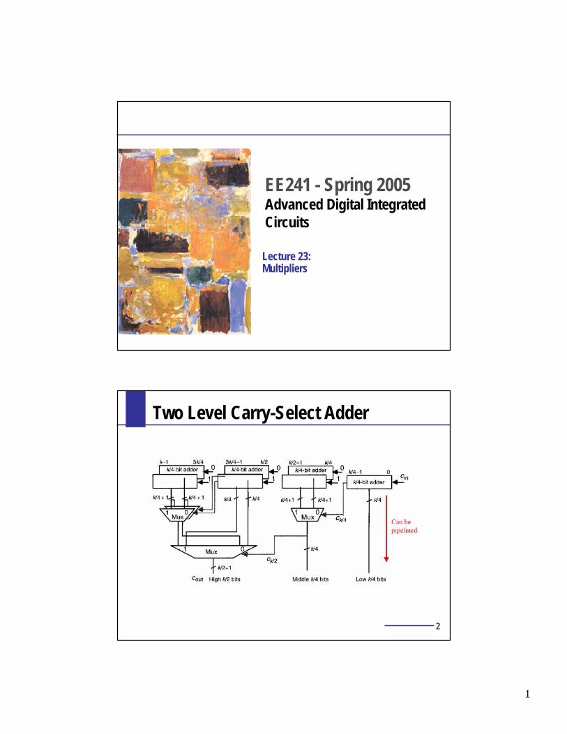
Two Level Carry-Select Adder

2

3

Conditional Sum Adders

4

TG Conditional Sum

Conditional CellConditional Sum Adder

2-way MUXes

Rothermel, JSSC 89

3

5

Carry-Lookahead Adders

Adder treesRadix of a tree

Minimum depth trees

Sparse trees

Logic manipulationsConventional vs. Ling

Stack height limiting

6

Propagate and Generate Signals

Define 3 new variables that ONLY depend on ai, bi

Generate (gi) = aibi

Propagate (pi) = ai + bi (could be XOR as well)

Delete = ai bi

Can also derive expressions for s and cout based on di

and pi

( )iniii

iniiiiout

cgpgs

cpgpgc

⊕=+=

),(

,

4

7

A0,B0 A1,B1 AN-1,BN-1...

Ci,0 P0 Ci,1 P1Ci,N-1 PN-1

...

Carry Lookahead Adder

Weinberger, Smith, 1958.

8

Lookahead Adder

1−+= iiii cpgc

Looakahead Equations

( )1111

111

111

−+++

−++

+++

++=++=

+=

iiiiii

iiiii

iiii

cppgpg

cpgpg

cpgc

Position i:

Position i + 1:

Carry exists if:- generated in stage i + 1- generated in stage i and propagated through i + 1- propagated through both i and i + 1

5

9

Lookahead Adder

• Unrolling of carry recurrence can be continued• If unrolled to level k, resulting in two-level AND-OR

structure• AND Fan-In = k + 1, OR Fan-In = k + 1• k + 1 transistors in the MOS stack• Limits k to 2 – 4 • Later referred to as a radix of an adder

10

Lookahead Adder

VDD

P3

P2

P1

P0

G3

G2

G1

G0

Ci,0

Co,3

Mirror Implementation

6

11

Block Lookahead

1123123

1232334

−++++++

+++++++++

++=

iiiiiiiii

iiiiiii

cppppgppp

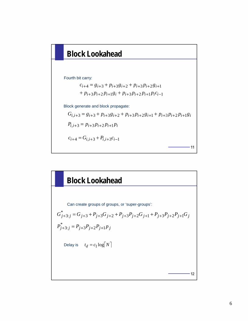
gppgpgcFourth bit carry:

iiiiiiiiiiii gpppgppgpgG 1231232333, ++++++++++ +++=

iiiiii ppppP 1233, ++++ =

13,3,4 −+++ += iiiiii cPGc

Block generate and block propagate:

12

Block Lookahead

Can create groups of groups, or ‘super-groups’:

jjjjjjjjjjjj GPPPGPPGPGG 123123233*

:3 ++++++++++ +++=

jjjjjj pPPPP 123*

:3 ++++ =

Delay is ⎡ ⎤Nctd log1=

7

13

Block Lookahead

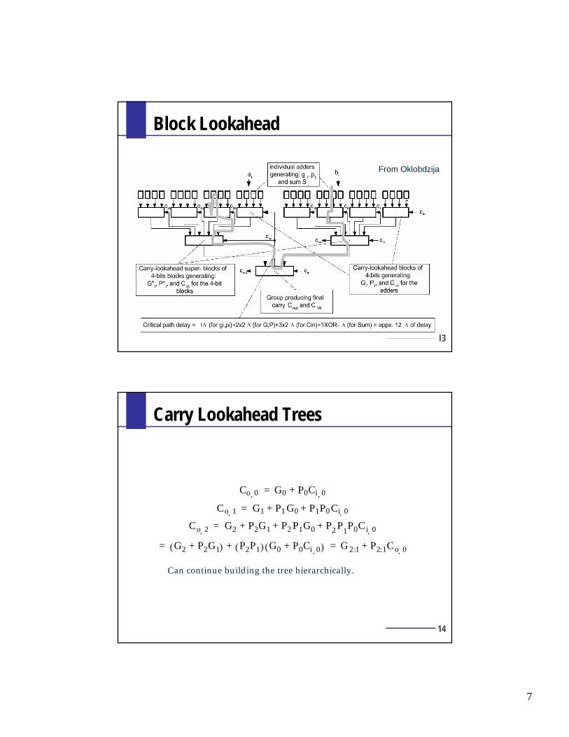
From Oklobdzija

14

Carry Lookahead Trees

Co 0, G0 P0Ci 0,+=

Co 1, G1 P1 G0 P1P0 Ci 0,+ +=

Co 2, G2 P2G1 P2 P1G0 P+ 2 P1P0Ci 0,+ +=

G2 P2G1+( )= P2P1( ) G0 P0Ci 0,+( )+ G 2:1 P2:1Co 0,+=

Can continue building the tree hierarchically.

8

15

Tree Adders

lmG ppP ⋅=

lmmG gpgG ⋅+=

m – more significantl – less significant

Start from the input P, G, and continue up the tree2-bit groups, then 4-bit groups, …

( ) ( ) ( )lmlmmllmm ppgpgpgpgpg ⋅⋅+=•= ,,,),(

Kogge, Stone, Trans on Comp,’73 Radix 2

16

Tree Adders: Radix 2

16-bit radix-2 Kogge-Stone Tree

(A0,

B0)

(A1,

B1)

(A2,

B2)

(A3,

B3)

(A4,

B4)

(A5,

B5)

(A6,

B6)

(A7,

B7)

(A8,

B8)

(A9,

B9)

(A10

, B10

)

(A11

, B11

)

(A12

, B12

)

(A13

, B13

)

(A14

, B14

)

(A15

, B15

)

S0

S1

S2

S3

S4

S5

S6

S7

S8

S9

S10

S11

S12

S13

S14

S15

9

17

Tree Adders: Radix 4

(a0, b

0)

(a1, b

1)

(a2, b

2)

(a3, b

3)

(a4, b

4)

(a5, b

5)

(a6, b

6)

(a7, b

7)

(a8, b

8)

(a9, b

9)

(a1

0,

b1

0)

(a1

1,

b1

1)

(a1

2,

b1

2)

(a1

3,

b1

3)

(a1

4,

b1

4)

(a1

5,

b1

5)

S0

S1

S2

S3

S4

S5

S6

S7

S8

S9

S1

0

S1

1

S1

2

S1

3

S1

4

S1

5

16-bit radix-4 Kogge-Stone Tree

18

Sparse Trees

(a0,

b0)

(a1,

b1)

(a2,

b2)

(a3,

b3)

(a4,

b4)

(a5,

b5)

(a6,

b6)

(a7,

b7)

(a8,

b8)

(a9,

b9)

(a10

, b1

0)

(a11

, b1

1)

(a12

, b1

2)

(a13

, b1

3)

(a14

, b1

4)

(a15

, b1

5)

S1

S3

S5

S7

S9

S11

S13

S15

S0

S2

S4

S6

S8

S1

0

S1

2

S1

4

16-bit radix-2 sparse tree with sparseness of 2 (Han-Carlson)

10

19

Full vs. Sparse TreesSparse trees have less transistors, wires

Less power

Less input loadingRecovering missing carries

Ripple (extra gate delay)Precompute (extra fanout)

Complex precompute can get into the critical path

Adder Delay [FO4]

Tot

al T

rans

isto

r W

idth

[uni

t wid

th/b

it]300

400

500

600

700

800

900

1000

7 9 11 13 15 17

Radix-4 Kogge-Stone

Radix-4 2-Sparse

Radix-4 4-Sparse

-23.3%

20

Tree Adders: Other Trees

Ladner-Fischer

(A0,

B0)

(A1,

B1)

(A2,

B2)

(A3,

B3)

(A4,

B4)

(A5,

B5)

(A6,

B6)

(A7,

B7)

(A8,

B8)

(A9,

B9)

(A10

, B10

)

(A11

, B11

)

(A12

, B12

)

(A13

, B13

)

(A14

, B14

)

(A15

, B15

)

S0

S1

S2

S3

S4

S5

S6

S7

S8

S9

S10

S11

S12

S13

S14

S15

11

21

Ling Adder

Variation of CLA

Ling, IBM J. Res. Dev, 5/81

1−⋅+= iiii GpgG

1−⊕= iii GpS

iii bap ⊕=

iii bag ⋅=

11 −− ⋅+= iiii HtgH

11 −−+⊕= iiiiii HtgHtS

iii bat +=

iii bag ⋅=

Ling’s equations

22

Ling Adder

1−⋅+= iiii GpgG

1−⋅+= iiii GtgG 11 −− ⋅+= iiii GtgH

Ling’s equation shifts the index ofpseudo carry

Doran, Trans on Comp 9/88

Propagates informationon two bits

Conventional CLA:

Also:

12

23

Ling Adder

01231232333 gtttgttgtgG +++=

0121223

00121122233

gttgtgg

gtttgttgtgH

+++=+++=

Conventional radix-4

Ling radix-4

Reduces the stack height (or width)Reduces input loading

24

Ling vs. CLA

10

15

20

25

30

35

40

45

50

55

60

6 7 8 9 10 11

Delay [FO4]

En

erg

y [p

J]

R2 Ling

R2 CLA

R4 Ling

R4 CLA

R. Zlatanovici, ESSCIRC’03

13

25

Static vs. Dynamic

8

13

18

23

28

33

38

5 7 9 11 13 15

Delay [FO4]

En

erg

y [p

J]Compound Domino R2

Domino R2

Domino R4Static R2

26

Stack Height Limiting

Transform conventional G, P

Park, VLSI Circ’00

14

27

HP Adder

Naffziger, ISSCC’96

01234 ppppi =

28

HP Adder – Differential Domino

Carry rippleSum select

15

29

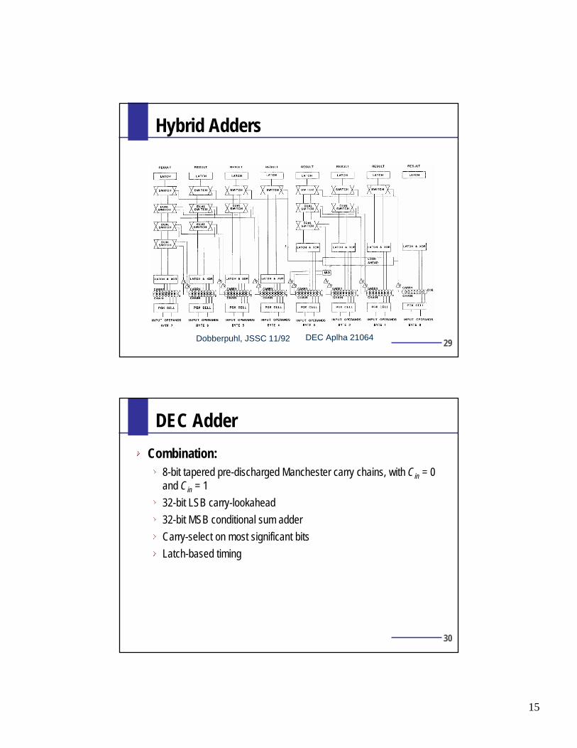
Hybrid Adders

Dobberpuhl, JSSC 11/92 DEC Aplha 21064

30

DEC Adder

Combination:8-bit tapered pre-discharged Manchester carry chains, with Cin = 0 and Cin = 1

32-bit LSB carry-lookahead

32-bit MSB conditional sum adder

Carry-select on most significant bits

Latch-based timing

16

31

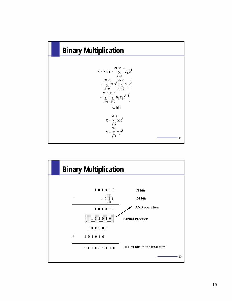
Z X·· Y× Zk2k

k 0=

M N 1–+

∑= =

Xi2i

i 0=

M 1–

∑⎝ ⎠⎜ ⎟⎜ ⎟⎜ ⎟⎛ ⎞

Yj2j

j 0=

N 1–

∑⎝ ⎠⎜ ⎟⎜ ⎟⎜ ⎟⎛ ⎞

=

XiYj2i j+

j 0=

N 1–

∑⎝ ⎠⎜ ⎟⎜ ⎟⎜ ⎟⎛ ⎞

i 0=

M 1–

∑=

X Xi2i

i 0=

M 1–

∑=

Y Yj2j

j 0=

N 1–

∑=

with

Binary Multiplication

32

1 0 1 1

1 0 1 0 1 0

0 0 0 0 0 0

1 0 1 0 1 0

1 0 1 0 1 0

1 0 1 0 1 0

×

1 1 1 0 0 1 1 1 0

+

Partial Products

AND operation

Binary Multiplication

N+ M bits in the final sum

N bits

M bits

17

33

Shift-and-Add Multiplier

Standard adder and shift-in the multiplicand

Shift the result as well and add

N cycles

Parallel adders add more hardware (adders) instead.

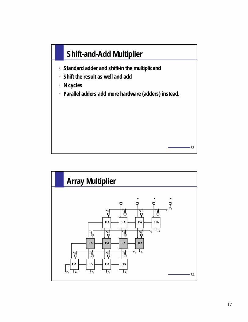
34

HA FA FA HA

FA FA FA HA

FA FA FA HA

X0X1X2X3 Y1

X0X1X2X3 Y2

X0X1X2X3 Y3

Z1

Z2

Z3Z4Z5Z6

Z0

Z7

Array Multiplier

18

35

HA FA FA HA

HAFAFAFA

FAFA FA HA

Critical Path 1

Critical Path 2

Critical Path 1 & 2

MxN Array Multiplier— Critical Path

36

HA HA HA HA

FAFAFAHA

FAHA FA FA

FAHA FA HA

Vector Merging Adder

Carry-Save Multiplier

19

37

SCSCSCSC

SCSCSCSC

SCSCSCSC

SC

SC

SC

SC

Z0

Z1

Z2

Z3Z4Z5Z6Z7

X0X1X2X3

Y1

Y2

Y3

Y0

Vector Merging Cell

HA Multiplier Cell

FA Multiplier Cell

X and Y signals are broadcastedthrough the complete array.( )

Multiplier Floorplan

38

Multipliers

Partial product generation

Partial product accumulation

Final summation

20

39

Generating Partial Products

All partial products: AND

Booth’s recoding – reduction of partial product count

X7

PP7

X6

PP6

X5

PP5

X4

PP4

X3

PP3

X2

PP2

X1

PP1

X0

PP0

40

Booth Recoding

Instead of generating all the partial products0 * x = 0 1 * x = x x={0,1}

Reduce the number of partial productsby grouping

0 0 00 1 1*1 0 2* (shift)1 1 3* (or 4* -1)

Booth’51

21

41

Booth Recoding

Instead of using set {0, 1*Y, 2*Y, 3*Y}

Use {0, 1*Y, 2*Y, 4*Y, -Y}

Shifting and complementing

3*Y = 4*Y – Y

Can be simplified by looking into three bits –modified Booth recoding

42

Modified Booth Recoding

Two bits and the MSB of previous two

22

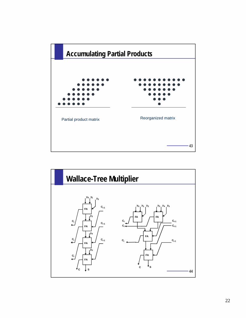
43

Accumulating Partial Products

Partial product matrix Reorganized matrix

44

FA

FA

FA

FA

y0 y1 y2

y3

y4

y5

S

Ci-1

Ci-1

Ci-1

Ci

Ci

Ci

FA

y0 y1 y2

FA

y3 y4 y5

FA

FA

CC S

Ci-1

Ci-1

Ci-1

Ci

Ci

Ci

Wallace-Tree Multiplier

23

45


46

Wallace-Tree

24

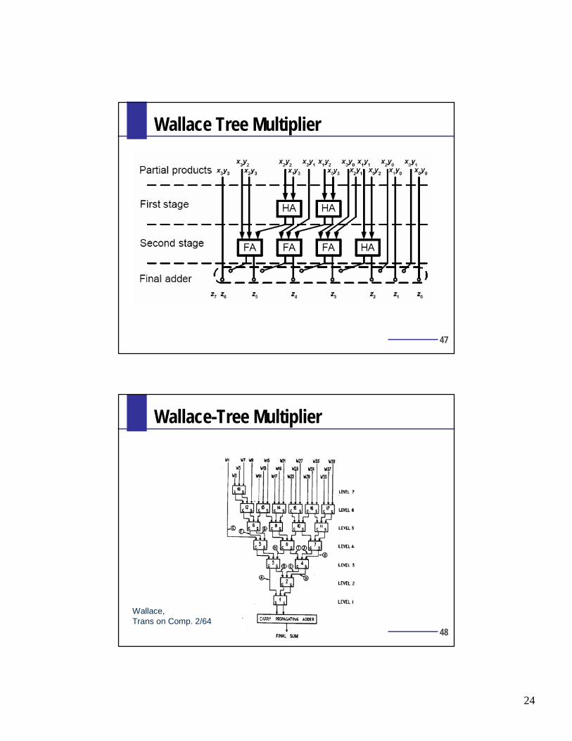
47

Wallace Tree Multiplier

48


Wallace,Trans on Comp. 2/64

25

49

Tree Multipliers

Time is proportional to log N

Wiring is complicated

Different wire lengths

Optional pipelining

Wallace tree: reduce the number of operands at earliest opportunityDadda tree: reduce the number of operands with fewest adders

50

Minimum Number of Stages

Dadda,`65

26

51

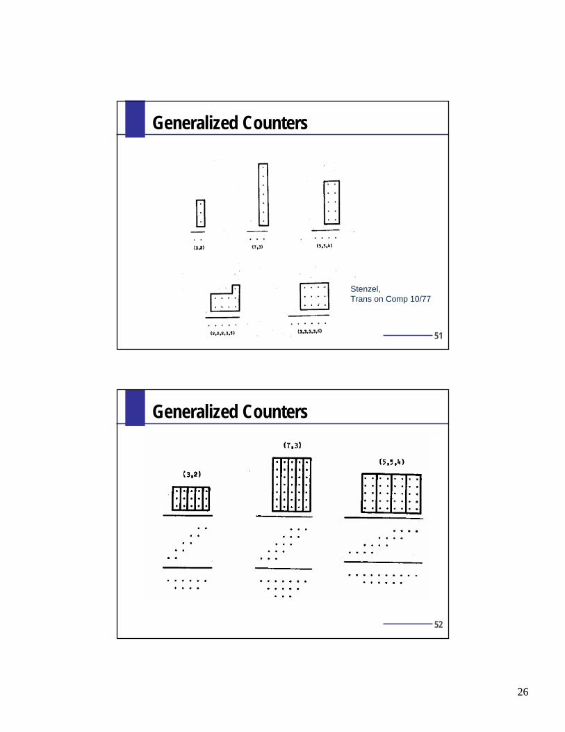
Generalized Counters

Stenzel,Trans on Comp 10/77

52


27

53


32x32busing (5,5,4)with (3,2) inthe last stage

54

4:2 Counters (Compressors)

Weinberger, IBM J. ResDev 1/81Santoro, Horowitz, JSSC 4/89

4-2 carry-save module

28

55

4:2 Compressors

Built of CSAsPipelined version compresses8 partial products per cycle

56

4:2 Compressors

Interconnect can be more regular than in Wallace tree

29

57

Three Dimensional Optimization

Oklobdzija, Villeger, Liu, Trans on Comp 3/96

58

Vertical Slices in TDM

30

59

Final Addition

60

Final Addition

31

61

Final Addition

62

Example: CPL Multiplier

BlockDiagram

CriticalPath

Yano,JSSC 4/90

32

63

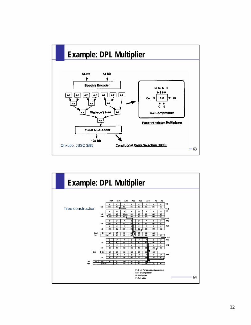
Example: DPL Multiplier

Ohkubo, JSSC 3/95

64


Tree construction

33

65


Final adder

66

Regularly Structured Tree

Goto, JSSC 9/92

34

67


68


35

69


Itoh, JSSC 2/01

two level carry-select...

Documents