two hybrid stepper motor models -...

Two Hybrid Stepper Motor Models

Dragoş DEACONU, Aurel CHIRILĂ, Valentin NĂVRĂPESCU, Mihaela ALBU, Constantin GHIŢĂ and Claudia POPESCU

University Politehnica of Bucharest – Electrical Engineering Department, 313, Splaiul Independenţei, Bucharest, Romania

Abstract - The paper is focused on the modeling and simulation of a Hybrid Step Motor (HSM). Starting from a real life HSM and using information from technical literature two HSM models have been developed. The first of them is used to analyze HSM’s response to different types of commands. The second model is used for the HSM’s electromagnetic field analysis. Key-Words: - Stepper motor, hybrid steppers, modelling, simulation 1. Introduction

Hybrid Step Motors (HSM) or Hybrid Stepper Motors as they are generally referred in the technical literature are commonly used in high precision dc electrical drives applications. A HSM combines the advantages of a Variable Reluctance Motor (VRM) and a Permanent Magnet Motor (PMM). As a result a HSM has the movement precision of a VRM and the torque of a PMM.

The main components of a HSM are the stator and the rotor. Usually the stator is made of toothed magnetic poles on which windings are placed (wounded stator) and the rotor is made of different magnetic cores (also toothed) that are separated by permanent magnets.

HSM manufacturers usually provide only a few of the motor’s parameters such as: rated power, rated voltage, rated current and the step angle. In order to properly design an industrial electrical drive a lot of other parameters are needed (such as: inertial moment, detent torque, electrical phase resistance, phase inductance etc.). In some cases it is difficult to identify these parameters therefore it is not easy to develop precise HSM models.

This paper shows two HSM models. One refers to the dynamic behavior of the motor and the other one to the electromagnetic field quantities within the motor.

2. Hybrid Step Motor Models A. The Modeled HSM

In this case the modeled HSM is one of the main components of a large knitting equipment.

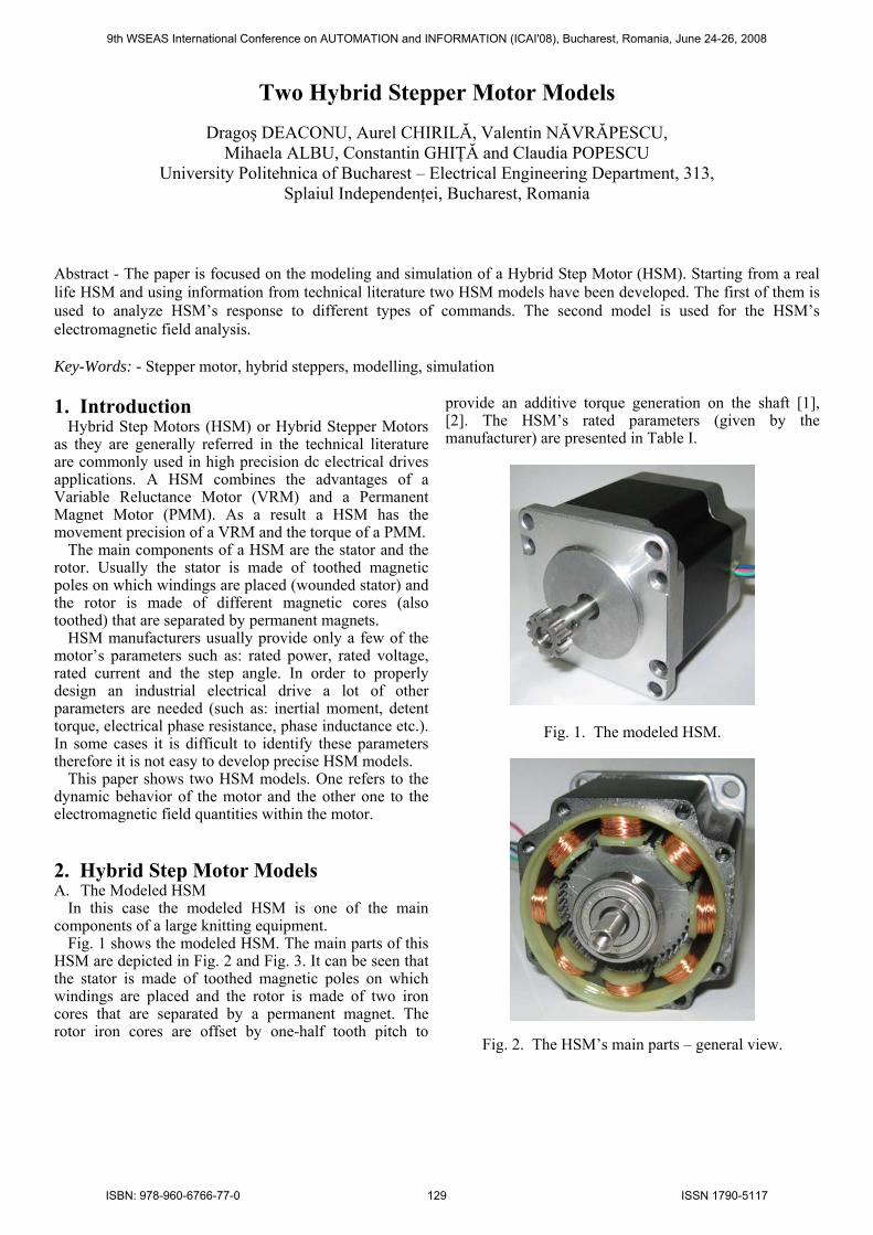
Fig. 1 shows the modeled HSM. The main parts of this HSM are depicted in Fig. 2 and Fig. 3. It can be seen that the stator is made of toothed magnetic poles on which windings are placed and the rotor is made of two iron cores that are separated by a permanent magnet. The rotor iron cores are offset by one-half tooth pitch to

provide an additive torque generation on the shaft [1], [2]. The HSM’s rated parameters (given by the manufacturer) are presented in Table I.

Fig. 1. The modeled HSM.

Fig. 2. The HSM’s main parts – general view.

9th WSEAS International Conference on AUTOMATION and INFORMATION (ICAI'08), Bucharest, Romania, June 24-26, 2008

ISBN: 978-960-6766-77-0 129 ISSN 1790-5117

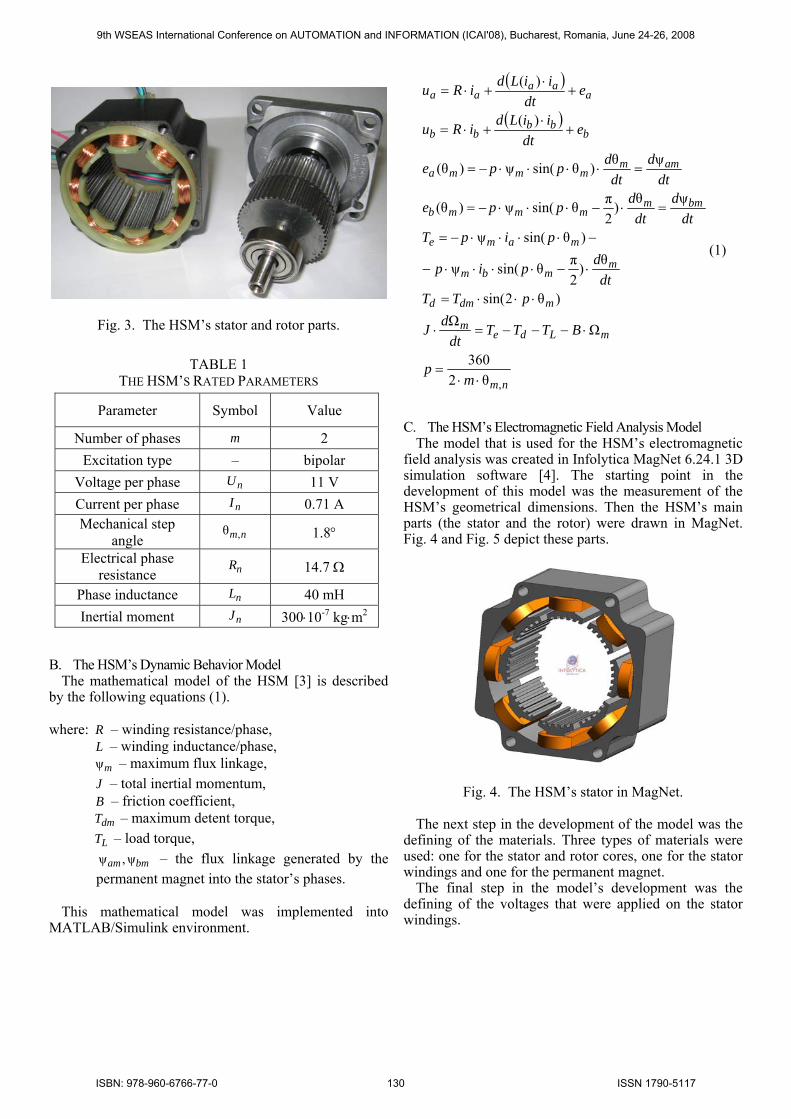
Fig. 3. The HSM’s stator and rotor parts.

TABLE 1 THE HSM’S RATED PARAMETERS

Parameter Symbol Value

Number of phases m 2 Excitation type – bipolar

Voltage per phase nU 11 V Current per phase nI 0.71 A Mechanical step

angle nm,θ 1.8°

Electrical phase resistance nR 14.7 Ω

Phase inductance nL 40 mH Inertial moment nJ 300⋅10-7 kg⋅m2

B. The HSM’s Dynamic Behavior Model The mathematical model of the HSM [3] is described

by the following equations (1).

where: R – winding resistance/phase, L – winding inductance/phase, mψ – maximum flux linkage, J – total inertial momentum, B – friction coefficient, dmT – maximum detent torque, LT – load torque,

bmam ψ,ψ – the flux linkage generated by the permanent magnet into the stator’s phases.

This mathematical model was implemented into MATLAB/Simulink environment.

( )

( )

nm

mLdem

mdmd

mmbm

mame

bmmmmmb

ammmmma

bbb

bb

aaa

aa

mp

BTTTdt

dJ

pTTdt

dpip

pipTdt

ddt

dppe

dtd

dtdppe

edt

iiLdiRu

edt

iiLdiRu

,θ2360

ΩΩ)θ2sin(

θ)2πθsin(ψ

)θsin(ψ

ψθ)2πθsin(ψ)θ(

ψθ)θsin(ψ)θ(

)(

)(

⋅⋅=

⋅−−−=⋅

⋅⋅⋅=

⋅−⋅⋅⋅⋅−

−⋅⋅⋅⋅−=

=⋅−⋅⋅⋅−=

=⋅⋅⋅⋅−=

+⋅

+⋅=

+⋅

+⋅=

(1)

C. The HSM’s Electromagnetic Field Analysis Model The model that is used for the HSM’s electromagnetic

field analysis was created in Infolytica MagNet 6.24.1 3D simulation software [4]. The starting point in the development of this model was the measurement of the HSM’s geometrical dimensions. Then the HSM’s main parts (the stator and the rotor) were drawn in MagNet. Fig. 4 and Fig. 5 depict these parts.

Fig. 4. The HSM’s stator in MagNet. The next step in the development of the model was the

defining of the materials. Three types of materials were used: one for the stator and rotor cores, one for the stator windings and one for the permanent magnet.

The final step in the model’s development was the defining of the voltages that were applied on the stator windings.


ISBN: 978-960-6766-77-0 130 ISSN 1790-5117

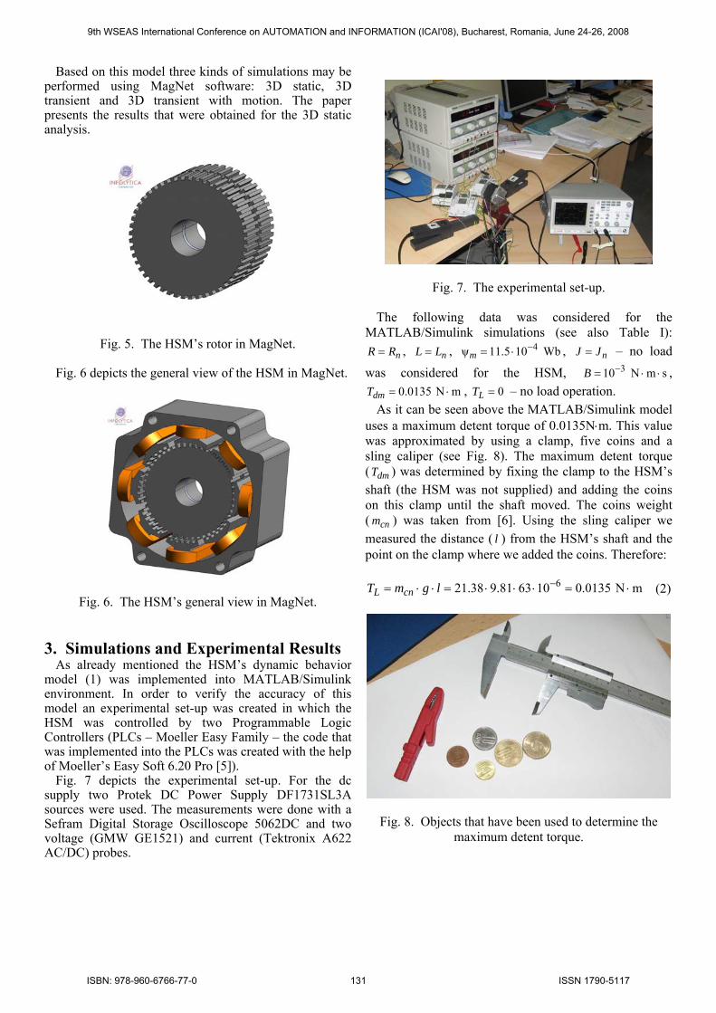
Based on this model three kinds of simulations may be performed using MagNet software: 3D static, 3D transient and 3D transient with motion. The paper presents the results that were obtained for the 3D static analysis.

Fig. 5. The HSM’s rotor in MagNet. Fig. 6 depicts the general view of the HSM in MagNet.

Fig. 6. The HSM’s general view in MagNet.

3. Simulations and Experimental Results As already mentioned the HSM’s dynamic behavior

model (1) was implemented into MATLAB/Simulink environment. In order to verify the accuracy of this model an experimental set-up was created in which the HSM was controlled by two Programmable Logic Controllers (PLCs – Moeller Easy Family – the code that was implemented into the PLCs was created with the help of Moeller’s Easy Soft 6.20 Pro [5]).

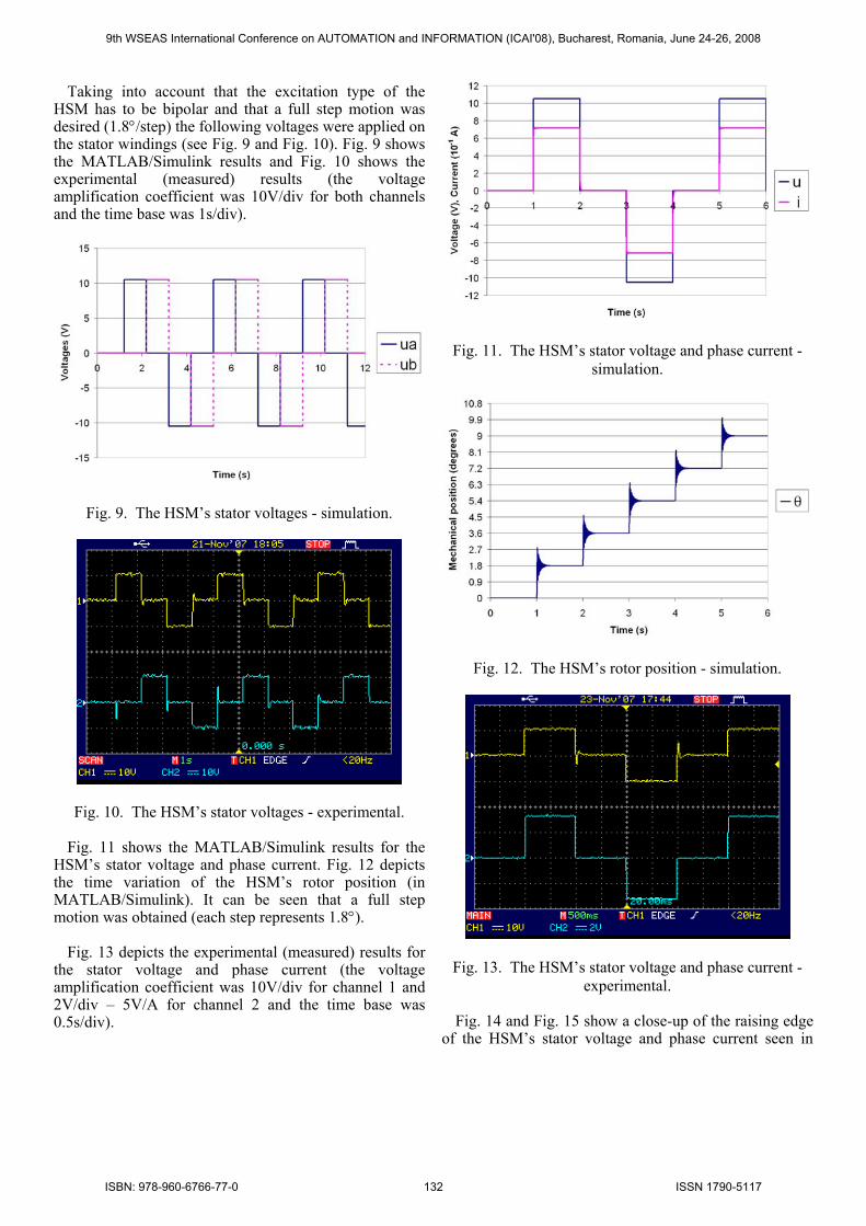
Fig. 7 depicts the experimental set-up. For the dc supply two Protek DC Power Supply DF1731SL3A sources were used. The measurements were done with a Sefram Digital Storage Oscilloscope 5062DC and two voltage (GMW GE1521) and current (Tektronix A622 AC/DC) probes.

Fig. 7. The experimental set-up. The following data was considered for the

MATLAB/Simulink simulations (see also Table I):

nRR = , nLL = , Wb105.11ψ 4−⋅=m , nJJ = – no load was considered for the HSM, smN10 3 ⋅⋅= −B ,

mN0135.0 ⋅=dmT , 0=LT – no load operation. As it can be seen above the MATLAB/Simulink model

uses a maximum detent torque of 0.0135N⋅m. This value was approximated by using a clamp, five coins and a sling caliper (see Fig. 8). The maximum detent torque ( dmT ) was determined by fixing the clamp to the HSM’s shaft (the HSM was not supplied) and adding the coins on this clamp until the shaft moved. The coins weight ( cnm ) was taken from [6]. Using the sling caliper we measured the distance ( l ) from the HSM’s shaft and the point on the clamp where we added the coins. Therefore:

mN0135.0106381.938.21 6 ⋅=⋅⋅⋅=⋅⋅= −lgmT cnL (2)

Fig. 8. Objects that have been used to determine the maximum detent torque.


ISBN: 978-960-6766-77-0 131 ISSN 1790-5117

Taking into account that the excitation type of the HSM has to be bipolar and that a full step motion was desired (1.8°/step) the following voltages were applied on the stator windings (see Fig. 9 and Fig. 10). Fig. 9 shows the MATLAB/Simulink results and Fig. 10 shows the experimental (measured) results (the voltage amplification coefficient was 10V/div for both channels and the time base was 1s/div).

Fig. 9. The HSM’s stator voltages - simulation.

Fig. 10. The HSM’s stator voltages - experimental. Fig. 11 shows the MATLAB/Simulink results for the

HSM’s stator voltage and phase current. Fig. 12 depicts the time variation of the HSM’s rotor position (in MATLAB/Simulink). It can be seen that a full step motion was obtained (each step represents 1.8°).

Fig. 13 depicts the experimental (measured) results for

the stator voltage and phase current (the voltage amplification coefficient was 10V/div for channel 1 and 2V/div – 5V/A for channel 2 and the time base was 0.5s/div).

Fig. 11. The HSM’s stator voltage and phase current - simulation.

Fig. 12. The HSM’s rotor position - simulation.

Fig. 13. The HSM’s stator voltage and phase current - experimental.

Fig. 14 and Fig. 15 show a close-up of the raising edge

of the HSM’s stator voltage and phase current seen in


ISBN: 978-960-6766-77-0 132 ISSN 1790-5117

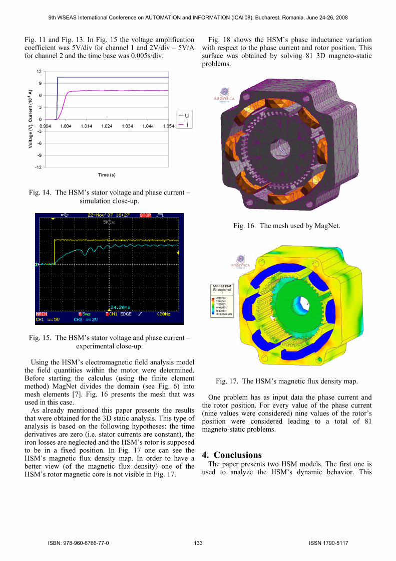
Fig. 11 and Fig. 13. In Fig. 15 the voltage amplification coefficient was 5V/div for channel 1 and 2V/div – 5V/A for channel 2 and the time base was 0.005s/div.

Fig. 14. The HSM’s stator voltage and phase current – simulation close-up.

Fig. 15. The HSM’s stator voltage and phase current – experimental close-up.

Using the HSM’s electromagnetic field analysis model

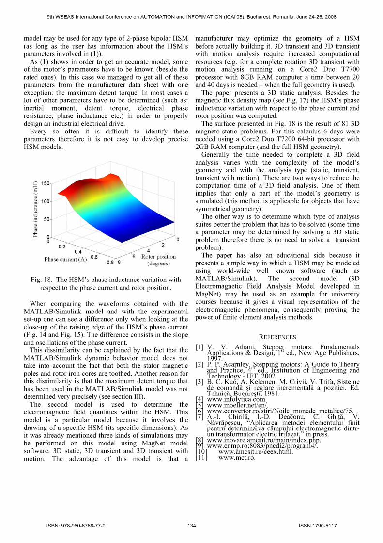
the field quantities within the motor were determined. Before starting the calculus (using the finite element method) MagNet divides the domain (see Fig. 6) into mesh elements [7]. Fig. 16 presents the mesh that was used in this case.

As already mentioned this paper presents the results that were obtained for the 3D static analysis. This type of analysis is based on the following hypotheses: the time derivatives are zero (i.e. stator currents are constant), the iron losses are neglected and the HSM’s rotor is supposed to be in a fixed position. In Fig. 17 one can see the HSM’s magnetic flux density map. In order to have a better view (of the magnetic flux density) one of the HSM’s rotor magnetic core is not visible in Fig. 17.

Fig. 18 shows the HSM’s phase inductance variation with respect to the phase current and rotor position. This surface was obtained by solving 81 3D magneto-static problems.

Fig. 16. The mesh used by MagNet.

Fig. 17. The HSM’s magnetic flux density map. One problem has as input data the phase current and

the rotor position. For every value of the phase current (nine values were considered) nine values of the rotor’s position were considered leading to a total of 81 magneto-static problems.

4. Conclusions The paper presents two HSM models. The first one is

used to analyze the HSM’s dynamic behavior. This


ISBN: 978-960-6766-77-0 133 ISSN 1790-5117

model may be used for any type of 2-phase bipolar HSM (as long as the user has information about the HSM’s parameters involved in (1)).

As (1) shows in order to get an accurate model, some of the motor’s parameters have to be known (beside the rated ones). In this case we managed to get all of these parameters from the manufacturer data sheet with one exception: the maximum detent torque. In most cases a lot of other parameters have to be determined (such as: inertial moment, detent torque, electrical phase resistance, phase inductance etc.) in order to properly design an industrial electrical drive.

Every so often it is difficult to identify these parameters therefore it is not easy to develop precise HSM models.

Fig. 18. The HSM’s phase inductance variation with respect to the phase current and rotor position.

When comparing the waveforms obtained with the

MATLAB/Simulink model and with the experimental set-up one can see a difference only when looking at the close-up of the raising edge of the HSM’s phase current (Fig. 14 and Fig. 15). The difference consists in the slope and oscillations of the phase current.

This dissimilarity can be explained by the fact that the MATLAB/Simulink dynamic behavior model does not take into account the fact that both the stator magnetic poles and rotor iron cores are toothed. Another reason for this dissimilarity is that the maximum detent torque that has been used in the MATLAB/Simulink model was not determined very precisely (see section III).

The second model is used to determine the electromagnetic field quantities within the HSM. This model is a particular model because it involves the drawing of a specific HSM (its specific dimensions). As it was already mentioned three kinds of simulations may be performed on this model using MagNet model software: 3D static, 3D transient and 3D transient with motion. The advantage of this model is that a

manufacturer may optimize the geometry of a HSM before actually building it. 3D transient and 3D transient with motion analysis require increased computational resources (e.g. for a complete rotation 3D transient with motion analysis running on a Core2 Duo T7700 processor with 8GB RAM computer a time between 20 and 40 days is needed – when the full geometry is used).

The paper presents a 3D static analysis. Besides the magnetic flux density map (see Fig. 17) the HSM’s phase inductance variation with respect to the phase current and rotor position was computed.

The surface presented in Fig. 18 is the result of 81 3D magneto-static problems. For this calculus 6 days were needed using a Core2 Duo T7200 64-bit processor with 2GB RAM computer (and the full HSM geometry).

Generally the time needed to complete a 3D field analysis varies with the complexity of the model’s geometry and with the analysis type (static, transient, transient with motion). There are two ways to reduce the computation time of a 3D field analysis. One of them implies that only a part of the model’s geometry is simulated (this method is applicable for objects that have symmetrical geometry).

The other way is to determine which type of analysis suites better the problem that has to be solved (some time a parameter may be determined by solving a 3D static problem therefore there is no need to solve a transient problem).

The paper has also an educational side because it presents a simple way in which a HSM may be modeled using world-wide well known software (such as MATLAB/Simulink). The second model (3D Electromagnetic Field Analysis Model developed in MagNet) may be used as an example for university courses because it gives a visual representation of the electromagnetic phenomena, consequently proving the power of finite element analysis methods.

REFERENCES [1] V. V. Athani, Stepper motors: Fundamentals

Applications & Design, 1st ed., New Age Publishers, 1997.

[2] P. P. Acarnley, Stepping motors: A Guide to Theory and Practice, 4th ed., Institution of Engineering and Technology - IET, 2002.

[3] B. C. Kuo, A. Kelemen, M. Crivii, V. Trifa, Sisteme de comandă şi reglare incrementală a poziţiei, Ed. Tehnică, Bucureşti, 1981.

[4] www.infolytica.com. [5] www.moeller.net/en/. [6] www.convertor.ro/stiri/Noile_monede_metalice/75. [7] A.-I. Chirilă, I.-D. Deaconu, C. Ghiţă, V.

Năvrăpescu, “Aplicarea metodei elementului finit pentru determinarea câmpului electromagnetic dintr-un transformator electric trifazat,” in press.

[8] www.inovare.amcsit.ro/main/index.php. [9] www.cnmp.ro:8083/pncdi2/program4/. [10] www.amcsit.ro/ceex.html. [11] www.mct.ro.


ISBN: 978-960-6766-77-0 134 ISSN 1790-5117

two hybrid stepper motor models -...

Documents