two-dimensional static deformation of an anisotropic medium

Sadhana Vol. 30, Part 4, August 2005, pp. 565–583. © Printed in India

Two-dimensional static deformation of an anisotropicmedium

KULDIP SINGH1, DINESH KUMAR MADAN2, ANITA GOEL3

and NAT RAM GARG3

1Department of Mathematics, Guru Jambheshwar University, Hisar 125 001, India2Department of Mathematics, T.I.T. & S., Bhiwani 127 021, India3Department of Mathematics, Maharshi Dayanand University, Rohtak 124 001,Indiae-mail: [email protected]

MS received 13 August 2004; revised 28 April 2005

Abstract. The problem of two-dimensional static deformation of a monoclinicelastic medium has been studied using the eigenvalue method, following a Fouriertransform. We have obtained expressions for displacements and stresses for themedium in the transformed domain. As an application of the above theory, the par-ticular case of a normal line-load acting inside an orthotropic elastic half-space hasbeen considered in detail and closed form expressions for the displacements andstresses are obtained. Further, the results for the displacements for a transverselyisotropic as well as for an isotropic medium have also been derived in the closedform. The use of matrix notation is straightforward and avoids unwieldy mathe-matical expressions. To examine the effect of anisotropy, variations of dimension-less displacements for an orthotropic, transversely isotropic and isotropic elasticmedium have been compared numerically and it is found that anisotropy affectsthe deformation significantly.

Keywords. Static deformation; anisotropic; orthotropic; monoclinic elasticmedium.

1. Introduction

Maruyama (1966) obtained closed-form expressions for the displacement and stress fields ina homogeneous isotropic elastic half-space as a result of line-source. Dziewonski & Anderson(1981) have established that the upper part of the earth is anisotropic. Laminated compositeanisotropic materials find a large number of engineering applications. Generalization of thesolution to include anisotropy is, however, very difficult. For a transversely isotropic medium,some other relevant contribution are those of Small & Booker (1984) and Pan (1989).

Chou (1976) and Ting (1995) discussed antiplane strain deformation of an anisotropicmedium. Garg et al (1996) obtained representations of seismic sources causing antiplanestrain deformations of orthotropic media. The corresponding plane strain deformation of an

565

566 Kuldip Singh et al

orthotropic elastic medium has been discussed by Garg et al (2003) using an eigenvalueapproach. Orthotropic symmetry is exhibited by olivine and orthopyroxens, the principal rockforming minerals of the deep crust and upper mantle.

In the present paper, a novel analytical eigenvalue method is presented for a monoclinicsolid. Fourier transformation of the equations of equilibrium for plane strain deformation of amonoclinic solid reduces them into a single linear homogeneous vector differential equation ofsecond order, on which an eigenvalue method is applied to obtain a solution in the transformeddomain. The form of the single governing equation for a monoclinic solid derived in this paperis a new contribution to the theory of monoclinic solids. The procedure developed in this paperis relatively simple and straightforward, avoids the cumbersome nature of the problem andis also convenient for numerical computation. As particular cases, normal line-loads actinginside orthotropic, transversely isotropic and perfectly isotropic elastic half-spaces have beenconsidered in detail. The deformation at any point of the medium is useful to analyse thedeformation field around mining tremors and drilling into the crust of the earth. It may alsofind application in various engineering problems, crystal physics and solid-earth geophysicsregarding deformation of an anisotropic solid. In fact, the study of a single force acting on amonoclinic solid forms the basis for further investigations such as dipolar sources and faultsin an anisotropic solid.

2. Basic equations and theory

The equations of equilibrium in the cartesian co-ordinate system (x1, x2, x3) for zero bodyforces are

τij,j = 0, (1)

where τij (i, j = 1, 2, 3) are the components of the stress tensor.The stress–strain relations for a monoclinic elastic medium, with x1x2-plane as a plane of

elastic symmetry are

τ11 = d11e11 + d12e22 + d13e33 + 2d16e12, (2)

τ22 = d12e11 + d22e22 + d23e33 + 2d26e12, (3)

τ33 = d13e11 + d23e22 + d33e33 + 2d36e12, (4)

τ23 = 2d44e23 + 2d45e13, (5)

τ13 = 2d45e23 + 2d55e13, (6)

τ12 = d16e11 + d26e22 + d36e33 + 2d66e12, (7)

where eij are the components of strain tensor and are related to displacement components(u1, u2, u3) through the relations

eij = 1/2(ui,j + uj,i). (8)

The two-suffix symmetric quantities dlk(l, k = 1, 2, . . . , 6) are the elastic moduli for amonoclinic elastic medium. For an orthotropic solid with coordinate planes coinciding withthe planes of symmetry, we have

d16 = d26 = d36 = d45 = 0, (9)

Deformation of an anisotropic medium 567

and the number of independent elastic coefficients reduce to nine. A transversely isotropicmedium is a particular case of orthotropy in which

d22 = d11, d23 = d13, d55 = d44, d66 = 1/2(d11 − d12), (10)

and there are five independent elastic coefficients. Further, isotropy is also a particular caseof an orthotropy in which

d11 = d22 = d33 = λ + 2µ,

d12 = d13 = d23 = λ,

d44 = d55 = d66 = µ, (11)

where λ and µ are Lame’ constants. For convenience, we shall write

(x1, x2, x3) = (x, y, z) and (u1, u2, u3) = (u, v, w).

We now consider the plane-strain deformation, parallel to the xy-plane, in which the dis-placement components are independent of z and are of the type

u = u(x, y), v = v(x, y), w = 0. (12)

The non-zero stresses for the plane-strain problem for a monoclinic medium are obtainedfrom (2)–(8), (10) and (12), as

τ11 = d11∂u

∂x+ d12

∂ v

∂y+ d16

(∂u

∂y+ ∂ v

∂x

), (13)

τ22 = d12∂u

∂x+ d22

∂ v

∂y+ d26

(∂u

∂y+ ∂ v

∂x

), (14)

τ33 = d13∂u

∂x+ d23

∂v

∂y+ d36

(∂u

∂y+ ∂v

∂x

), (15)

τ12 = d16∂u

∂x+ d26

∂v

∂y+ d66

(∂u

∂y+ ∂v

∂x

). (16)

The equations of equilibrium, for a plane-strain deformation (parallel to the xy-plane) of amonoclinic elastic medium are[

d11∂2u

∂x2+ d66

∂2u

∂y2+ 2d16

∂2u

∂x∂y

]

+[d16

∂2v

∂x2+ d26

∂2v

∂y2+ (d12 + d66)

∂2v

∂x∂y

]= 0, (17)

[d16

∂2u

∂x2+ d26

∂2u

∂y2+ (d66 + d12)

∂2u

∂x∂y

]

+[d66

∂2v

∂x2+ d22

∂2v

∂y2+ 2d26

∂2v

∂x∂y

]= 0, (18)


We define the following dimensionless quantities,

α = x

h, β = y

h, U = u

h, V = v

h, σ11 = τ11

d66, σ12 = τ12

d66, σ22 = τ22

d66,

a = d11

d66, b = d22

d66, c = d12

d66, d = d26

d66, e = d16

d66, (19)

where ‘h’ is a known fixed quantity and has the dimensions of length. Thus, the equations ofequilibrium (17) and (18), in dimensionless form become[

a∂2U

∂α2+ ∂2U

∂β2+ 2e

∂2U

∂α∂β

]+[e∂2V

∂α2+ d

∂2V

∂β2+ (c + 1)

∂2V

∂α∂β

]= 0, (20)

[e∂2U

∂α2+ d

∂2U

∂β2+ (1 + c)

∂2U

∂α∂β

]+[∂2V

∂α2+ b

∂2V

∂β2+ 2d

∂2V

∂α∂β

]= 0. (21)

In (20) and (21), α is the dimensionless vertical distance, β is the dimensionless horizontaldistance, U is the dimensionless vertical displacement, V is the dimensionless horizontaldisplacement, σ11, σ12, σ22 are the dimensionless stress components, and a, b, c, d, e aredimensionless elastic coefficients.

For an isotropic solid,

a = b = 1/(1 − α∗), c = (1 − 2α∗)/(α∗ − 1) = a − 2, d = 0, e = 0, (22)

where

α∗ = (λ + µ)/(λ + 2µ), (23)

in particular, for a Poissonian isotropic solid (λ = µ), and α∗ = 2/3.We define the Fourier transform f (α, k) of a function f (α, β) by the relation

f (α, k) = F [f (α, β)] =∫ +∞

−∞f (α, β)eιkβdβ, (24)

so that

f (α, β) = (1/2π)

∫ ∞

−∞f (α, k)e−ιkβdk, (25)

where k is the Fourier transform parameter.Applying the Fourier transformation on equations of equilibrium (20) and (21), we find[

ad2U

dα2− 2eιk

dU

dα− k2U

]+[e

d2V

dα2− ιk(1 + c)

dV

dα− dk2V

]= 0, (26)

[e

d2U

dα2− ιk(1 + c)

dU

dα− k2dU

]+[

d2V

dα2− 2dιk

dV

dα− bk2V

]= 0. (27)

The above two equations can be written as the following single homogeneous vector dif-ferential equation:

A◦ d2N0

dα2+ B◦ dN0

dα+ C◦N0 = 0, (28)


where

A◦ =[a e

e 1

], B◦ =

[ −2 ιke −ιk(1 + c)

−ιk(1 + c) −2ιkd

],

C◦ =[

−k2 −k2d

−k2d −bk2

], N0 =

[U

V

]. (29)

We note that matrices A◦, B◦ and C◦ are all symmetric, matrix A◦ depends upon dimensionlesselastic moduli while the matrices B◦ and C◦ depend upon parameter k also. The governingequation (28) for a monoclinic solid is a new contribution and eigenvalue method shall beapplied to solve the problem. For this, we seek a solution of vector differential equation (28)of the type

N0(α, k) = E(k)esα, (30)

where s is a parameter and E(k) is a matrix of the type 2 × 1. Substitution of the value of N0

from (30) into vector differential equation (28) gives the following characteristic equation:

a0s4 + 4a1s

3 + 6a2s2 + 4a3s + a4 = 0, (31)

where

a0 = a − e2, a1 = −ι (ad − ce)k/2,

a2 = −(ab − c2 − 2c + 2ed)k2

6,

a3 = 2ι(cd − be)k3

4, a4 = (b − d2)k4. (32)

To solve biquadratic equation (31), we make use of Descartes’ method, in which the secondterm is removed by using the transformation

z∗ = a0s + a1, (33)

so that (31) reduces to

(z∗)4 + 6H(z∗)2 + 4Gz∗ + (a20I − 3H 2) = 0, (34)

where

H = a0a2 − a21, G = a2

0a3 − 3a0a1a2 + 2a31,

I = a0a4 − 4a1a3 + 3a22 . (35)

Following Descartes’ method, the left hand side of (34) can be resolved into a product of twoquadratic factors as

(z∗)4 + 6H(z∗)2 + 4Gz∗ + (a20I − 3H 2)

= [(z∗)2 + p0z∗ + q][(z∗)2 − p0z

∗ + q′], (36)


where

q + q′ = p20 + 6H, qq′ = a2

0I − 3H 2, (37)

p0(q′ − q) = 4G. (38)

when p0 = 0, the values of q and q′ are determined from (37) directly, otherwise, eliminatingq and q′ from (37) and (38), we get

ξ 3 + 3b1ξ2 + 3b2ξ + b3 = 0, (39)

where

ξ = p20, b1 = 4H,

b2 = 4(12H 2 − a20I )/3, b3 = −16G2. (40)

Equation (39) is a cubic in ξ and hence, can be solved using Cardan’s method and thus (39)is reduced to

δ3 + 3H1δ + G1 = 0, (41)

where

δ = ξ + b1, H1 = b2 − b21, G1 = b3 − 3b1b2 + 2b3

1. (42)

The roots of the cubic equation (41) are

δ = u0 + v0, (43)

where u0 and v0 are given by

u30 =

−G1 +√

G21 + 4H 3

1

2, v3

0 =−G1 −

√G2

1 + 4H 31

2, (44)

satisfying u0v0 = −H1. Then p0 is given by

p20 = δ − b1, (45)

and q and q′ are then to be calculated from (37), (38) and (45). Equation (36) gives

z∗1 = −p0 + (p2

0 − 4q)1/2

2, z∗

2 = −p0 − (p20 − 4q)1/2

2,

z∗3 = p0 + (p2

0 − 4q ′)1/2

2, z∗

4 = p0 − (p20 − 4q ′)1/2

2, (46)

as the roots of the biquadratic equation (34). Hence, the eigenvalues of the problem ares1, s2, s3, s4, where

sL = z∗L − a1

a0, for L = 1, 2, 3, 4. (47)


The eigenvectors for a monoclinic elastic medium are obtained by solving the matrix equation

[s2A◦ + sB◦ + C◦]E(k) = 0, (48)

and the eigenvectors are found to be

XTL = [P1L, 1], for L = 1, 2, 3, 4, (49)

where

P1L = −[es2L − ιksL(1 + c) − k2d]

as2L − 2ιkesL − k2

= −[s2L − 2ιkdsL − bk2]

es2L − ιksL(1 + c) − k2d

(50)

and (. . . )T denote the transpose of the matrix (. . . ). Thus, a general solution of the vector-matrix differential equation (28) for a monoclinic elastic medium for non-repeated eigenvaluesis of the form

N0(α, k) =4∑

L=1

(BLXLesLα), (51)

where coefficients B1, B2, B3 and B4 are to be determined from prescribed boundary condi-tions. These coefficients may depend upon k. Equation (51) gives the following expressionsfor the dimensionless displacements in the transformed domain.

U (α, k) = B1P11es1α + B2P12e

s2α + B3P13es3α + B4P14e

s4α,

V (α, k) = B1es1α + B2e

s2α + B3es3α + B4e

s4α. (52)

Further, the expressions for dimensionless stresses for a plane strain deformation for a mon-oclinic solid are found to be

σ11 = [Q11B1es1α + Q12B2e

s2α + Q13B3es3α + Q14B4e

s4α],

σ12 = [R11B1es1α + R12B2e

s2α + R13B3es3α + R14B4e

s4α], (53)

where

Q1L = aP1LsL − ιkc − ιkeP1L + sLe,

R1L = eP1LsL − ιkd − ιkP1L + sL for L = 1, 2, 3, 4. (54)

3. Particular cases

3.1 Orthotropic symmetry

In this case

d = 0, e = 0, a1 = 0, a3 = 0, (55)

and vector differential equation and characteristics equation for an orthotropic medium areobtained from (28), (29), (31), (32) and (55). We find

Ad2N

dα2+ B

dN

dα+ CN = 0, (56)


in which A, B, C are

A =(

a 00 1

), B =

(0 −ιk(1 + c)

−ιk(1 + c) 0

),

C =(

−k2 0

0 −bk2

), N =

(U

V

), (57)

and

as4 − (ab − c2 − 2c)k2s2 + bk4 = 0. (58)

The characteristic equation (58) is a quadratic equation in s2 and can be solved directlywithout using Descartes’ method and gives the eigenvalues as

s2 = m21k

2, m22k

2, (59)

where

m21 = A0 + (A2

0 − 4B0)1/2

2, m2

2 = A0 − (A20 − 4B0)

1/2

2,

A0 = (ab − c2 − 2c)/a = m21 + m2

2, B0 = b/a = m21m

22. (60)

Under the assumption that m1 �= m2, the eigenvalues are

s1 = m1|k|, s2 = m2|k|,s3 = −m1|k|, s4 = −m2|k|, (61)

with real parts of (m1, m2) as positive.The eigenvectors for an orthotropic elastic medium are given by

XTL = [P2L, 1], XT

L+2 = [−P2L, 1], (62)

for L = 1, 2, in which

P21 = ιm1|k|k

(1 + c

am21 − 1

)= ιk

m1|k|(

b − m21

1 + c

),

P22 = ιm2|k|k

(1 + c

am22 − 1

)= ιk

m2|k|(

b − m22

1 + c

), (63)

Thus, a solution of matrix equation (56) for the case of an orthotropic elastic medium is

N(α, k) =2∑

L=1

[(CLXLemL|k|α + CL+2XL+2e−mL|k|α], (64)

where the coefficients C1, C2, C3 and C4 are to be determined from boundary conditions andthey may depend upon k.


The transformed dimensionless displacements for an orthotropic elastic medium are

U (α, k) = C1P21em1|k|α + C2P22e

m2|k|α − C3P21e−m1|k|α − C4P22e

−m2|k|α,

V (α, k) = C1em1|k|α + C2e

m2|k|α + C3e−m1|k|α + C4e

−m2|k|α, (65)

and stresses in the transformed domain are

σ11(α, k) = Q21C1em1|k|α + Q22C2e

m2|k|α + Q21C3e−m1|k|α + Q22C4e

−m2|k|α,

σ12(α, k) = R21C1em1|k|α + R22C2e

m2|k|α − R21C3e−m1|k|α − R22C4e

−m2|k|α,

(66)

where

Q2L = aP2LmL|k| − ιck,

R2L = mL|k| − ιP2Lk, for L = 1, 2. (67)

3.2 Transversely isotropic symmetry

This case is a particular case of monoclinic symmetry as well as orthotropic symmetry andhere the dimensionless elastic constants are

a = b = 2

(d11

d11 − d12

), c = 2

(d12

d11 − d12

)= a − 2, d = e = 0. (68)

The characteristic equation for a transversely isotropic elastic medium becomes

s4 − 2k2s2 + k4 = 0, (69)

provided d11 �= 0 and d11 �= d12 and it is observed that this characteristic equation is indepen-dent of its elastic moduli a, b, c. The solution of characteristic equation (69) gives repeatedeigenvalues

s = s1 = s2 = −s3 = −s4 = |k|. (70)

The equilibrium equations in the transformed domain for a transversely isotropic mediumare equivalent to the first-order vector differential equation. Further treatment for this caseis different from the treatment discussed earlier for a orthotropic/monoclinic medium withdifferent eigenvalues.

Ross (1984) has given a procedure to tackle the problems with repeated eigenvalues pro-vided the governing vector differential equation is of the first-order. For this situation, wedefine the process as given by Ross (1984) and the first order vector differential equationrepresenting the equilibrium equations is

dN1/dα = A1N1, (71)

where

N1 =

U

V

dU

dα

dV

dα

, A1 =

0 0 1 0

0 0 0 1

k2

a0 0

ιk(a − 1)

a

0 ak2 ιk(a − 1) 0

(72)


Following the procedure as outlined by Ross (1984), the four independent eigen vectors arefound to be

X1 =

ι|k|k

ιk2

k|k|

, X2 =

ι

{|k|α −

(2a

a − 1

)}

k

(α − 1

|k|)

ι|k|{|k|α −

(1 + a

a − 1

)}k|k|α

,

X3 =

−ι|k|k

ιk2

−k|k|

, X4 =

−ι

{|k|α +

(2a

a − 1

)}

k

(α + 1

|k|)

ι|k|{|k|α +

(1 + a

a − 1

)}−k|k|α

(73)

Thus, a general solution of first order matrix differential equation (71) for a transverselyisotropic medium (Ross 1984) is

N1 = (D1X1 + D2X2)e|k|α + (D3X3 + D4X4)e

−|k|α, (74)

where D1, D2, D3, D4 are coefficients which may depend upon k and dimensionless elasticcoefficient a.

The displacements and stresses in the transformed domain for a transversely isotropicmedium are found to be

U = ι

[{D1|k| + D2

(|k|α − 2a

a − 1

)}e|k|α

−{D3|k| + D4

(|k|α + 2a

a − 1

)}e−|k|α

]

V = k

[{D1 + D2

(α − 1

|k|)}

e|k|α +{D3 + D4

(α + 1

|k|)}

e−|k|α]

(75)

σ11 = ι

[2k2D1e

|k|α +{

2k2α + |k|(

2 − 4a

a − 1

)}D2e

|k|α

+2k2D3e−|k|α +

{2k2α + |k|

(4a − 2

a − 1

)}D4e

−|k|α]

,

σ12 =[{

2k|k|D1 + D2

(2k|k|α − 2ak

a − 1

)}e|k|α

−{

2k|k|D3 + D4

(2k|k|α + 2ak

a − 1

)}e−|k|α

]. (76)


4. An application: A normal line-load in an elastic half-space

We consider an elastic half-space with x-axis vertically downwards and the origin of thecartesian coordinate system (x, y, z) is taken at the boundary of the half-space. Let a normalline-load P0 be acting vertically downwards on a line parallel to z-axis and passing through thepoint (H, 0). The bounding surface x = 0 is assumed to be stress-free and we shall calculatethe resulting stresses and displacements at any point of the half-space for the following threetypes of medium:

4.1 Deformation of an orthotropic elastic medium

Consider the elastic half-space consisting of region α < α0 (medium I) and region α > α0

(medium II). We find the displacements and stresses at any point of an orthotropic elastic half-space due to a normal line-load P0 acting vertically downwards on a line parallel to z-axis(figure 1).

The boundary conditions are:On the plane x = 0,

τ 111(x = 0, y) = 0, τ 1

12(x = 0, y) = 0. (77)

On the plane x = H ,

u1(x = H, y) = u2(x = H, y),

v1(x = H, y) = v2(x = H, y),

τ 112(x = H, y) = τ 2

12(x = H, y),

τ 211(x = H, y) − τ 1

11(x = H, y) = −P0δ(y), (78)

where δ(y) is the Dirac-delta function and F [δ(y)] = 1.Defining the dimensionless force

P = P0/d66. (79)

Let the coefficients C1, C2, C3, C4 appearing in (65) and (66) in medium I be represented byC1, C2, C3, C4 and for medium II be represented by C+

1 , C+2 , C+

3 , C+4 .

Figure 1. A normal line-load P0.


The corresponding response in medium I is

U 1(α, k) = C1P21em1|k|α + C2P22e

m2|k|α − C3P21e−m1|k|α − C4P22e

−m2|k|α,

V 1(α, k) = C1em1|k|α + C2e

m2|k|α + C3e−m1|k|α + C4e

−m2|k|α,

σ 111(α, k) = (aP21m1|k| − ιkc)(C1e

m1|k|α + C3e−m1|k|α)

+ (aP22m2|k| − ιkc)(C2em2|k|α + C4e

−m2|k|α),

σ 112(α, k) = (m1|k| − ιkP21)(C1e

m1|k|α − C3e−m1|k|α)

+ (m2|k| − ιkP22)(C2em2|k|α − C4e

−m2|k|α), (80)

and in medium II is given by,

U 2(α, k) = −C+3 P21e

−m1|k|α − C+4 P22e

−m2|k|α,

V 2(α, k) = C+3 e−m1|k|α + C+

4 e−m2|k|α,

σ 211(α, k) = (aP21m1|k| − ιkc)(C+

3 e−m1|k|α) + (aP22m2|k| − ιkc)(C+4 e−m2|k|α),

σ 212(α, k) = (m1|k| − ιkP21)C3e

−m1|k|α(m2|k| − ιkP22)C4e−m2|k|α. (81)

Applying the boundary conditions from (77)–(78) and using the matrix method, we obtainthe following values of coefficients.

C1 = M3/D5, C2 = −M3/D6,

C3 = −M3

M1

(M2

D5− 2D2D4

D6

), C4 = −M3

M1

(M2

D6− 2D1D3

D5

),

C+3 = −M3

D7

[1 + M2

M1

D7

D5− 2

M1

D2D4D7

D6

],

C+4 = M3

D8

[1 − M2

M1

D8

D6+ 2

M1

D1D3D8

D5

], (82)

where

D1 = aP21m1|k| − ιkc, D2 = aP22m2|k| − ιkc,

D3 = m1|k| − ιkP21, D4 = m2|k| − ιkP22,

D5 = em1|k|α0, D6 = em2|k|α0,

D7 = e−m1|k|α0, D8 = e−m2|k|α0 .

M1 = D1D4 − D2D3, M2 = D1D4 + D2D3,

M3 = P/2(D1 − D2). (83)


Putting values of the various coefficients from (82) into displacements and stresses obtainedin (80)–(81), we get the following expressions for displacements and stresses at any point ofan orthotropic elastic half-space in the transformed domain:

U (α, k) = P

2T1

[m1R1

1

|k|e−m1|k||α−α0| − m2R2

1

|k|e−m2|k||α−α0|

+ m1R1T3

T2

1

|k|e−m1|k| (α+α0) + m2R2T3

T2

1

|k|e−m2|k|(α+α0)

+ 2m1R1T4

T2

1

|k|e−|k|(m1α+m2α0) − 2m2R2T5

T2

1

|k|e−|k|(m2α+m1α0)

]

V (α, k) = P

2 ιT1

[±1

ke−m1|k||α−α0| ∓ 1

ke−m2|k||α−α0|

− T3

T2

1

ke−m1|k|(α+α0) − T3

T2

1

ke−m2|k|(α+α0)

+ 2T4

T2

1

ke−|k|(m1α+m2α0) + 2T5

T2

1

ke−|k|(m1α0+m2α)

],

σ11 = P

2T1

[± (am2

1R1 − c)e−m1|k||α−α0| ∓ (am22R2 − c)e−m2|k||α−α0|

− T3

T2(am2

1R1 − c)e−m1|k|(α+α0) − T3

T2(am2

2R2 − c)e−m2|k|(α+α0)

+ 2T4

T2(am2

1R1 − c)e−|k|(m1α+m2α0)

+ 2T5

T2(am2

2R2 − c)e−|k|(m2α+m1α0)

],

σ12 = ιP |k|T1k

[−m1

2(1 + R1)e

−m1|k||α−α0| + m2

2(1 + R2)e

−m2|k||α−α0|

− m1T3

2T2(1 + R1)e

−m1|k|(α+α0) − m2T3

2T2(1 + R2)e

−m2|k|(α+α0)

+ m1T4

T2(1 + R1)e

−|k|(m1α+m2α0)

+ m2T5

T2(1 + R2)e

−|k|(m2α+m1α0)

], (84)

where the upper sign is for the region α < α0 and lower sign is for the region α > α0, andα0 = H/h,

R1 = 1 + c

am21 − 1

, R2 = 1 + c

am22 − 1

, T1 = aR1(m22 − m2

1)

am22 − 1

,

T2 = (am1m2 + c)(m1R1 − m2R2) + (m1 − m2)am1m2R1R2 + (m1 − m2)c,

T3 = (am1m2 − c)(m1R1 + m2R2) + (m1 + m2)am1m2R1R2 − (m1 + m2)c,


T4 = (am22 − c)m2R2 + am3

2R22 − m2c,

T5 = (am21 − c)m1R1 + am3

1R21 − m1c. (85)

We note that quantities R1, R2, T1, T2, T3, T4 and T5 are independent of k. Taking inversionand using appendix A, we get the following closed-form expressions for the displacementsand stresses at any point of an orthotropic elastic half-space due to a normal line force actingat (H, 0).

U(α, β) = P

4πT1

[−m1R1 log{β2 + m2

1(α − α0)2}

+ m2R2 log{β2 + m22(α − α0)

2}

− m1R1T3

T2log{β2 + m2

1(α + α0)2}

− m2R2T3

T2log{β2 + m2

2(α + α0)2}

+ 2m1R1T4

T2log{β2 + (m1α + m2α0)

2}

+ 2m2R2T5

T2log{β2 + (m2α + m1α0)

2}]

,

V (α, β) = P

2πT1

[∓ tan−1

(β

m1|α − α0|)

± tan−1

(β

m2|α − α0|)

+ T3

T2tan−1

(β

m1(α + α0)

)+ T3

T2tan−1

(β

m2(α + α0)

)

− 2T4

T2tan−1

(β

|m1α + m2α0|)

− 2T5

T2tan−1

(β

m2α + m1α0

)],

σ11(α, β) = P

2πT1

[±(am2

1R1 − c)

{m1(α0 − α)

β2 + m21(α0 − α)2

}

∓ (am22R2 − c)

{m2|α − α0|

β2 + m22(α − α0)2

}

− T3

T2(am2

1R1 − c)

{m1(α + α0)

β2 + m21(α + α0)2

}

− T3

T2(am2

2R2 − c)

{m2(α + α0)

β2 + m22(α + α0)2

}

+ 2T4

T2(am2

1R1 − c)

{ |m1α + m2α0|β2 + (m1α + m2α0)2

}

+ 2T5

T2(am2

2R2 − c)

{ |m2α + m1α0|β2 + (m2α + m1α0)2

}],


σ12(α, β) = P

2πT1

[− m1(1 + R1)β

β2 + m21(α − α0)2

+ m2(1 + R2)β

β2 + m22(α − α0)2

− m1T3(1 + R1)β

T2{β2 + m21(α + α0)2} − m2T3(1 + R2)β

T2{β2 + m22(α + α0)2}

+ 2m1T4(1 + R1)β

T2{β2 + (m1α + m2α0)2} + 2m2T5(1 + R2)β

T2{β2 + (m2α + m1α0)2}]

. (86)

4.2 Deformation of a transversely isotropic elastic half-space

Following the same procedure, as adopted for an orthotropic case, we obtain the followingclosed-form expressions for displacements at any point of a transversely isotropic elastichalf-space due to a normal line-load acting at (H, 0).

U(α, β) = P

4π

[a − 1

a

{(α0 − α)2

β2 + (α0 − α)2

}−(

a + 1

2a

)log{β2 + (α0 − α)2}

+(a + 1

a

){(α0 + α)2

β2 + (α0 + α)2

}− 1

2a

(a2 + 1

a − 1

)log{β2 + (α0 + α)2}

+ 2

(a − 1

a

)α0α

{(α + α0)

2 − β2

((α + α0)2 + β2)2

}],

V (α, β) = P

4π

[−(

a − 1

a

)(α0 − α)

{β

β2 + (α0 − α)2

}

−(a + 1

a

)|α0 − α|

{β

β2 + (α0 + α)2

}−(

2

a − 1

)tan−1

(β

α + α0

)

+ 4αα0

(a − 1

a

){β(α + α0)

(β2 + (α0 + α)2)2

}]. (87)

4.3 Deformation of an isotropic elastic half-space

For an isotropic case a = 1/(1 − α∗), using this in (87), we obtain the following closed-form expressions for the displacements at any point of an isotropic elastic half-space due toa normal line-load acting at (H, 0).

U(α, β) = P

4π

[α∗(α0 − α)2

β2 + (α0 − α)2− (2 − α∗)

2log {β2 + (α0 − α)2}

+ (2 − α∗)(α0 + α)2

β2 + (α0 + α)2− 1

2

(2 − 2α∗ + α∗2

α∗

)log{β2 + (α0 + α)2)

+ 2α∗α0α

{(α + α0)

2 − β2

((α + α0)2 + β2)2

}],

V (α, β) = P

4π

[−α∗β(α0 − α)

β2 + (α0 − α)2− (2 − α∗)(α0 − α)β

β2 + (α0 + α)2

− 2

(1 − α∗

α∗

)tan−1

(β

α + α0

)+ 4α0αα∗β(α + α0)

{β2 + (α + α0)2)2

]. (88)


The displacements for an isotropic elastic half-space obtained in (88) coincide with the cor-responding results obtained by Maruyama (1966).

5. Numerical results and discussion

We wish to examine the effect of anisotropy of the elastic half-space. For numerical com-putations, we use the values of elastic constants given by Love (1944) for topaz material(orthotropic), which are

a = 2.15789, b = 2.67669, c = 0.96240.

To examine the effect of anisotropy of elastic medium, various distribution curves in figures 2to 5 are plotted for orthotropic, transversely isotropic and isotropic elastic medium. For atransversely isotropic medium, the following relations

b = a, c = a − 2

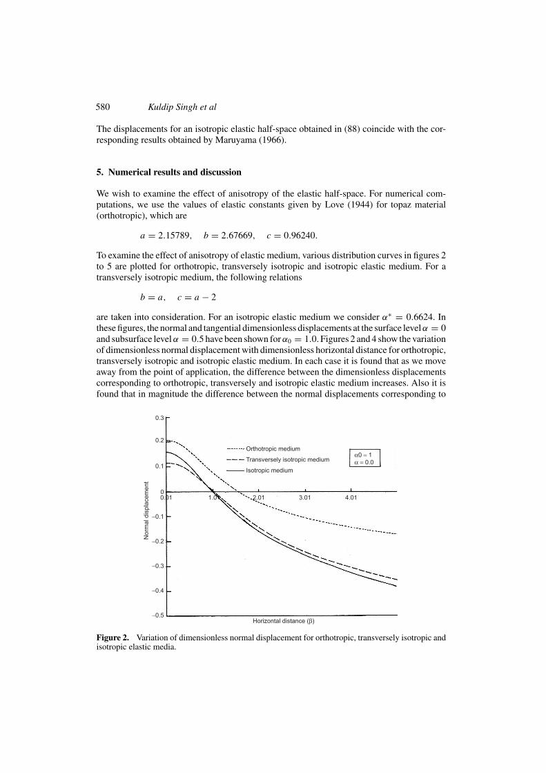
are taken into consideration. For an isotropic elastic medium we consider α∗ = 0.6624. Inthese figures, the normal and tangential dimensionless displacements at the surface levelα = 0and subsurface level α = 0.5 have been shown for α0 = 1.0. Figures 2 and 4 show the variationof dimensionless normal displacement with dimensionless horizontal distance for orthotropic,transversely isotropic and isotropic elastic medium. In each case it is found that as we moveaway from the point of application, the difference between the dimensionless displacementscorresponding to orthotropic, transversely and isotropic elastic medium increases. Also it isfound that in magnitude the difference between the normal displacements corresponding to

Figure 2. Variation of dimensionless normal displacement for orthotropic, transversely isotropic andisotropic elastic media.


Figure 3. Variation of dimensionless tangential displacement for orthotropic, transversely isotropicand isotropic elastic media.

Figure 4. Variation of dimensionless normal displacement for orthotropic, transversely isotropic andisotropic elastic media.


Figure 5. Variation of dimensionless tangential displacement distribution for orthotropic, transverselyisotropic and isotropic elastic media.

orthotropic and isotropic is greater than that of the difference between transversely isotropicand isotropic. Figures 3 and 5 show the variation of dimensionless tangential displacementwith dimensionless horizontal distance for orthotropic, transversely isotropic and isotropicelastic medium. As we move away from the point of application the difference betweenthe dimensionless tangential displacement corresponding to orthotropic and isotropic elasticmedium increases. While the difference between the dimensionless tangential displacementscorresponding to isotropic and transversely isotropic medium decreases.

From these figures, it is concluded that the anisotropy is affecting the deformation sub-stantially.

KS is grateful to the University Grants Commission, New Delhi for financial support.

Appendix (x > 0) A

(1)∫ ∞

−∞e−ι kydk = 2πδ(y)

(2)∫ ∞

∞(|k|)−1e−|k|xe−ιkydk = − log(y2 + x2)


(3)∫ ∞

−∞k−1e−|k|xe−ιkydk = −2ι tan−1

(y

x

)

(4)∫ ∞

−∞e−|k|xe−ιkydk = 2z

y2 + z2

(5)∫ ∞

−∞

k

|k|e−|k|xe−ιkydk = −2ιy

y2 + x2

(6)∫ ∞

−∞ke−|k|xe−ιkydk = −4 ιyx

(y2 + x2)2

(7)∫ ∞

−∞|k| e−|k|xe−ι kydk = 2(z2 − y2)

(z2 + y2)2

(8)∫ ∞

−∞k2 e−|k|ze−ιkydk = 4x(x2 − 3y2)

(x2 + y2)3

(9)∫ ∞

−∞k|k| e−|k|xe−ιkydk = −4 ιy(3z2 − y2)

(z2 + y2)3

References

Chou Y T 1976 On antiplane line force in a two-phase anisotropic medium. Phys. Stat. Sol. 34: 645–650

Dziewonski A M, Anderson D L 1981 Preliminary reference Earth model. Phys. Earth Planet. Inter.25: 297–356

Garg N R, Madan D K, Sharma R K 1996 Two-dimensional deformation of an orthotropic elasticmedium due to seismic sources. Phys. Earth Planet. Inter. 94: 43–62

Garg N R, Kumar R, Goel A, Miglani A 2003 Plane strain deformation of an orthotropic elasticmedium using an eigenvalue approach. Earth, Planets Space 55: 3–8

Maruyama T 1966 On two-dimensional elastic dislocations in an infinite and semi-infinite medium.Bull. Earthquake Res. Inst. 44: 811–871

Pan E 1989 Static response of a transversely isotropic and layered half-space to general dislocationsources. Phys. Earth Planet. Inter. 58: 103–117

Ross S L 1984 Differential equations 3rd edn (New York: John Wiley and Sons)Small J C, Booker J R 1984 Finite layer analysis of layered elastic materials using a flexibility approach,

Part I – strip loading. Int. J. Numer. Methods Engg. 21: 1025–1037Ting T C T 1995 Antiplane deformation of anisotropic elastic materials. In Recent advances in

elasticity, viscoelasticity and inelasticity: Series in advances in mathematics in applied sciences(ed.) K R Rajgopal (Singapore: World Scientific) 26: 150–179

two-dimensional static deformation of an anisotropic medium

Documents