two-dimensional relativistic longitudinal green s function ...timormel/index_files/linecurrent...

Two-dimensional relativistic longitudinal Green’sfunction in the presence of a moving planar

dielectric–magnetic discontinuity

Tatiana Danov and Timor Melamed*

Department of Electrical and Computer Engineering, Ben-Gurion University of the Negev, Beer Sheva 84105, Israel*Corresponding author: [email protected]

Received September 19, 2011; revised October 23, 2011; accepted October 26, 2011;posted October 26, 2011 (Doc. ID 154988); published February 14, 2012

The current contribution is concerned with obtaining the relativistic two-dimensional (three-dimensional in re-lativity jargon) Green’s function of a time-harmonic line current that is embedded in a moving dielectric–magneticmedium with a planar discontinuity. By applying a plane-wave (PW) spectral representation for the relativisticelectromagnetic Green’s function of a dielectric–magnetic medium that is moving in a uniform velocity, the exactreflected and transmitted (refracted) fields are obtained in the form of a spectral integral over PWs in the so-calledlaboratory and comoving frames. We investigate these spectral representations, as well as their asymptoticevaluations, and discuss the associated relativistic wave phenomena of direct reflected/transmitted rays andrelativistic head waves (lateral waves). © 2012 Optical Society of America

OCIS codes: 350.5720, 080.0080, 290.5825, 050.1960.

1. INTRODUCTION AND STATEMENT OFTHE PROBLEMGreen’s functions of electromagnetic (EM) wave propagationin a moving medium have been a subject of a continuingresearch [1–4]. The dyadic Green’s functions of an homoge-neous isotropic dielectric–magnetic medium have been de-rived in closed form in [5] and an alternative simplederivation was presented in [6].

Plane-wave (PW) spectral representations have been an im-portant tool for solving relativistic scattering and diffractionproblems. Such spectral representations have been utilizedfor scattering of a PW by a uniformly moving perfectly con-ducting half-plane [7], for the two-dimensional problem ofthe uniformly moving perfectly conducting cylinder [8], forsolving the EM field radiated by an infinitely long thin wireantenna that uniformly translates in a direction parallel toa plane interface [9], for the EM radiation from fractal anten-nas [10], and for EM wave scattering from moving roughsurfaces [11].

EM scattering from moving objects is of fundamentalimportance in antenna and scattering theory, cellular andsatellite communication, radar applications, inverse scatter-ing, remote sensing, and more. Although impressive advanceshave been made in this field, little effort has been made toadjust basic stationary wave theories [such as the geometricaltheory of diffraction (GTD), the uniform theory of diffraction,and direct time-domain methods] to the scatterer dynamics.Basic wave phenomena of relativistic scattering, such ashigh-frequency/short-pulsed canonical forms and diffractioncoefficients, are not yet fully understood. Furthermore, littleattention has been given to problems concerning scattering ina moving dielectric medium where the electrodynamics intro-duces wave phenomena that are unique to special relativityand that are not found in classical (stationary) GTD, suchas relativistic lateral waves and their wave phenomena,

Čerenkov-type scattering and its high-frequency forms,and more.

Recently, a PW spectral representation of the relativisticelectric and magnetic dyadic Green’s functions of a uniformlymoving dielectric–magnetic medium was obtained in [12]. Byapplying a simple coordinate transformation, scalarization ofthe EM vectorial problemwas obtained in which the EM dyadsare evaluated from Helmholtz’s free-space (isotropic) scalarGreen’s function. The spectral PW representations of the dya-dic Green’s functions were obtained by applying the spatialtwo-dimensional (2D) Fourier transform to the scalar Green’sfunction in both the under and over phase-speed mediumvelocity regimes.

In the current work, we apply the spectral representationsin [12] in order to obtain the EM Green’s function of a time-harmonic line current that is located at �y; z� � �0; 0� and isembedded in a uniformly moving dielectric–magnetic mediumwith a planar discontinuity. In K -frame, the medium is movingin a constant translation velocity v � vz, where we assumethat the velocity is in the direction of the z axis. Unit vectorsin the conventional Cartesian coordinate system, �x; y; z�, aredenoted by a hat over bold fonts. Under the framework of spe-cial relativity, a three-dimensional (space–time) event �y; z; t�in the so-called laboratory frame (K -frame) is mapped to theevent �y0; z0; t0� in the comoving frame (K 0-frame) by the Lor-entz transformation (LT) and the inverse LT (ILT), which aredefined for the K 0-frame velocity of v � vz by

y0 � y; z0 � γ�z − βct�; t0 � γ�t − βz∕c�; (1)

y � y0; z � γ�z0 � βct0�; t � γ�t0 � βz0∕c�; (2)

where c � 1∕��ϵ0μ0

pis the speed of light in vacuum and

T. Danov and T. Melamed Vol. 29, No. 3 / March 2012 / J. Opt. Soc. Am. A 285

1084-7529/12/030285-10$15.00/0 © 2012 Optical Society of America

β � v∕c; γ � 1∕��1 − β2

q: (3)

Here and henceforth, all physical quantities in the K 0-frameare denoted by a prime. The EM field transformation thatis corresponding to v � vz is given by [13]

E0�r0; t0� � V · �E� v × B�;B0�r0; t0� � V · �B − v × E∕c2�;D0�r0; t0� � V · �D� v ×H∕c2�;H0�r0; t0� � V · �H − v × D�; (4)

where r0 � �y0; z0�, the r � �y; z� and t coordinates are trans-formed into �r0; t0� via ILT in Eq. (2), and the (diagonal) dyadicV is given by

V � diagfγ; γ; 1g: (5)

Here and henceforth, underlined boldfaced letters denote ma-trices/dyads. The inverse of Eq. (4) is form invariant and thuscan be obtained by interchanging all primed and unprimedquantities where V0 � V and v0 � −v.

We are aiming at obtaining the relativistic 2D (3D in rela-tivity jargon) Green’s function of the time-harmonic linecurrent,

J�r; t� � I0δ�z�δ�y� exp�jωt�x; (6)

that is located in the so-called laboratory K -frame at r ��y; z� � �0; 0� (see Fig. 1). The source is embedded in a uni-formly moving dielectric–magnetic medium with a planardiscontinuity. The medium’s discontinuity is located at z �z0 > 0 at time t � 0 in K -frame. The medium is assumed tobe a linear isotropic dielectric–magnetic in the frame at rest(the “comoving” K 0-frame) with ϵ01;2 and μ01;2 denoting itspermittivity and permeability, where indices 1 and 2 referto either side of the discontinuity. Thus, the constitutive rela-tions in K 0-frame are

D0 � ϵ01E0; B0 � μ01H0; z0 < z00;

D0 � ϵ02E0; B0 � μ02H0; z0 > z00; (7)

where z00 � γz0 denotes the interface location in K 0-frame,which is obtained from LT in Eq. (1). In the current contribu-tion, we assume that the medium is lossless and dispersionfree and that its velocity does not exceed the K 0-frame phase

velocities of c∕��ϵ01;2μ01;2

q.

The outline of the paper is as follows: in Section 2 we brieflydescribe the spectral representation of the incident field thatwas derived in [12] and, in Section 3, the spectral representa-tion of the Green’s function in the presence of a movingdiscontinuity is obtained by applying Maxwell’s boundaryconditions in K 0-frame. The spectral representation isobtained in both K 0- and K -frames of reference inSubsections 3.A and 3.B, respectively. The asymptotic evalua-tions of the incident, reflected, and transmitted (refracted)waves in the high-frequency regime are obtained in Sections 4and 5 for fields in K 0- and K -frames, respectively.

2. SPECTRAL REPRESENTATION OF THEINCIDENT FIELDThe incident EM field in K -frame is the field that is radiated bythe current line source in Eq. (6). The line current is em-bedded in a uniformly moving dielectric–magnetic mediumof (K 0) permittivity and permeability of ε01 and μ01, respectively(for all r0). In K -frame, the corresponding constitutive rela-tions can be stated as [6]

D � ϵ01α · E� c−1mz ×H;

B � μ01α ·H − c−1mz × E; (8)

where

m � β n021 − 1

1 − n021 β2

; n01 � c

��ϵ01μ01

p; (9)

and α is the diagonal matrix

α � diagfα; α; 1g; α � 1 − β21 − n02

1 β2: (10)

The spectral representation of the incident EM field that isdenoted by Ei�r; t� can be obtained by formulating the currentsource Green’s function in K 0-frame where the constitutive re-lations have simple expressions, while the source densityfunction involves distributions that are moving along the zaxis with velocity v (see, for example, [14]). In the current con-tribution we use the results that were obtained in [12] in whichthe incident EM field was derived directly in K -frame by usingthe normalized longitudinal coordinate and wavenumber

�z � ��α

pz; �k1 � ω

��αϵ01μ01

p: (11)

Note thatm in Eq. (9) and α in Eq. (10) are positive (assumingthat the medium velocity does not exceed the medium’s phasevelocity of c∕n0

1) so that��αp> 0 is real.

By using these definitions, the incident electric field isdecomposed into PWs in the form

Ei�r; t� � 12π

Zdky~E

i�r; t; ky�; (12)

where the incident electric field spectral PWs that are denotedby ~Ei are given by

~Ei�r; t; ky� � −I0ωμ01

��αp

2�kz1x exp�jΨi�;

Ψi � ωt − kyy − �kz1�z� kmz; (13)

Fig. 1. Physical configuration of the relativistic Green’s function of aline current that is embedded in a dielectric–magnetic medium with aplanar discontinuity. The medium is uniformly moving in the z direc-tion with a velocity of v � vz in the laboratory frame and the discon-tinuity is located in z � z0 at t � 0. The medium is an isotropicdielectric–magnetic in the comoving frame with ε01;2 and μ01;2 denotingits permittivity and permeability on either side of the discontinuity.

286 J. Opt. Soc. Am. A / Vol. 29, No. 3 / March 2012 T. Danov and T. Melamed

where k � ω∕c is the wavenumber in vacuum, and the long-itudinal wavenumber that is denoted by �kz1 is given by

�kz1 ��k21 − k2y

q; Re �kz1 ≥ 0; Im �kz1 ≤ 0. (14)

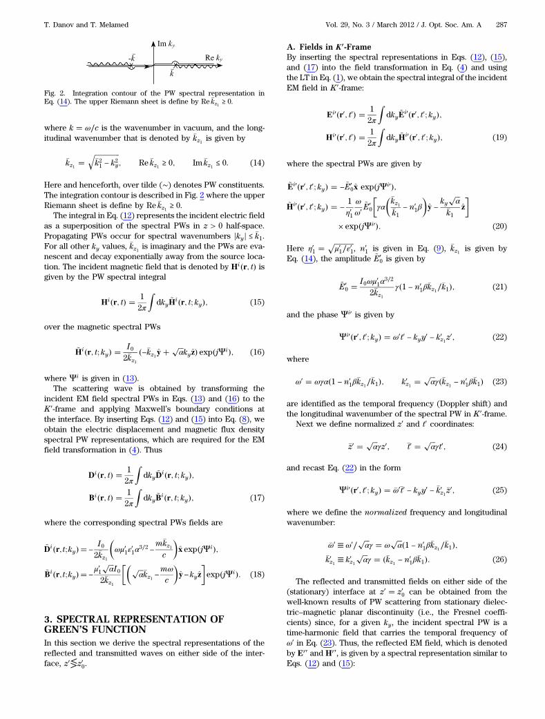
Here and henceforth, over tilde (∼) denotes PW constituents.The integration contour is described in Fig. 2 where the upperRiemann sheet is define by Re �kz1 ≥ 0.

The integral in Eq. (12) represents the incident electric fieldas a superposition of the spectral PWs in z > 0 half-space.Propagating PWs occur for spectral wavenumbers jkyj ≤ �k1.For all other ky values, �kz1 is imaginary and the PWs are eva-nescent and decay exponentially away from the source loca-tion. The incident magnetic field that is denoted by Hi�r; t� isgiven by the PW spectral integral

Hi�r; t� � 12π

Zdky ~H

i�r; t; ky�; (15)

over the magnetic spectral PWs

~Hi�r; t; ky� �I02�kz1

�−�kz1 y��α

pkyz� exp�jΨi�; (16)

where Ψi is given in (13).The scattering wave is obtained by transforming the

incident EM field spectral PWs in Eqs. (13) and (16) to theK 0-frame and applying Maxwell’s boundary conditions atthe interface. By inserting Eqs. (12) and (15) into Eq. (8), weobtain the electric displacement and magnetic flux densityspectral PW representations, which are required for the EMfield transformation in (4). Thus

Di�r; t� � 12π

Zdky ~D

i�r; t; ky�;

Bi�r; t� � 12π

Zdky~B

i�r; t; ky�; (17)

where the corresponding spectral PWs fields are

~Di�r; t;ky��−I02�kz1

�ωμ01ε01α3∕2 −

m�kz1c

�x exp�jΨi�;

~Bi�r; t;ky��−μ01

��αpI0

2�kz1

�� α

p�kz1 −

mωc

�y−kyz

�exp�jΨi�: (18)

3. SPECTRAL REPRESENTATION OFGREEN’S FUNCTIONIn this section we derive the spectral representations of thereflected and transmitted waves on either side of the inter-face, z0≶z00.

A. Fields in K0-FrameBy inserting the spectral representations in Eqs. (12), (15),and (17) into the field transformation in Eq. (4) and usingthe LT in Eq. (1), we obtain the spectral integral of the incidentEM field in K 0-frame:

Ei0�r0; t0� � 12π

Zdky~E

i0�r0; t0; ky�;

Hi0�r0; t0� � 12π

Zdky ~H

i0�r0; t0; ky�; (19)

where the spectral PWs are given by

~Ei0�r0; t0; ky� � −~E00x exp�jΨi0�;

~Hi0�r0; t0; ky� � −1η01

ωω0

~E00

�γα��kz1�k1

− n01β�y −

ky��αp

�k1z�

× exp�jΨi0�: (20)

Here η01 ��μ01∕ε01

p, n0

1 is given in Eq. (9), �kz1 is given byEq. (14), the amplitude ~E0

0 is given by

~E00 �

I0ωμ01α3∕22�kz1

γ�1 − n01β�kz1∕�k1�; (21)

and the phase Ψi0 is given by

Ψi0�r0; t0; ky� � ω0t0 − kyy0 − k0z1z0; (22)

where

ω0 � ωγα�1 − n01β�kz1∕�k1�; k0z1 �

��α

pγ��kz1 − n0

1β�k1� (23)

are identified as the temporal frequency (Doppler shift) andthe longitudinal wavenumber of the spectral PW in K 0-frame.

Next we define normalized z0 and t0 coordinates:

�z0 � ��α

pγz0; �t0 � ��

αp

γt0; (24)

and recast Eq. (22) in the form

Ψi0�r0; t0; ky� � �ω0�t0 − kyy0 − �k0z1�z0; (25)

where we define the normalized frequency and longitudinalwavenumber:

�ω0 ≡ ω0∕��α

pγ � ω

��α

p �1 − n01β�kz1∕�k1�;

�k0z1 ≡ k0z1��α

pγ � ��kz1 − n0

1β�k1�: (26)

The reflected and transmitted fields on either side of the(stationary) interface at z0 � z00 can be obtained from thewell-known results of PW scattering from stationary dielec-tric–magnetic planar discontinuity (i.e., the Fresnel coeffi-cients) since, for a given ky, the incident spectral PW is atime-harmonic field that carries the temporal frequency ofω0 in Eq. (23). Thus, the reflected EM field, which is denotedby Er0 and Hr0, is given by a spectral representation similar toEqs. (12) and (15):

Fig. 2. Integration contour of the PW spectral representation inEq. (14). The upper Riemann sheet is define by Re �kz1 ≥ 0.


Er0�r0; t0� � 12π

Zdky~E

r0�r0; t0; ky�;

Hr0�r0; t0� � 12π

Zdky ~H

r0�r0; t0; ky�; (27)

over their spectral PWs

~Er0�r0; t0; ky� � −~E00Γ0�ky�x exp�jΨr0�;

~Hr0�r0; t0; ky� �1η01

Γ0�ky�~E00γ−1�k1

ω�ω0 �k0z1 y� kyz� exp�jΨr0�: (28)

Here ω0 is given in Eq. (23) and the phase Ψr0 is given by

Ψr0�r0; t0; ky� � �ω0�t0 − kyy0 − �k0z1�2�z00 − �z0�; (29)

with �z0 in Eq. (24) and �z00 ��αp γz00. In Eq. (28), Γ0�ky� denotes

the Fresnel reflection coefficient [13]:

Γ0�ky� �μ02�k0z1 − μ01�k0z2μ02�k0z1 � μ01�k0z2

; (30)

where

�k0z2 ��ω02ε02μ02 − k2y∕αγ2

q; (31)

and �ω0 and �k0z1 are given in Eq. (26).Similarly, the transmitted field that is propagating in

z0 > z00 is given by the spectral integrations

Et0�r0; t0� � 12π

Zdky~E

t0�r0; t0; ky�;

Ht0�r0; t0� � 12π

Zdky ~H

t0�r0; t0; ky�; (32)

over the transmitted spectral PWs

~Et0�r0; t0; ky� � −~E00T

0�ky�x exp�jΨt0�;~Ht0�r0; t0; ky� � −

1ω0μ02

~E00T

0�ky��k0z2 y − kyz� exp�jΨt0�; (33)

where the phase Ψt0 is given by

Ψt0�r0; t0; ky� � �ω0�t0 − kyy0 − �k0z2 ��z0 − �z00� − �k0z1�z00; (34)

and the transmission coefficient T 0�ky� of the interface atz0 � z00 is given by

T 0�ky� � 1� Γ0�ky�: (35)

The spectral PWs in Eq. (33) are propagating in (y0; z0 > z0o)half-space in the direction of the unit vector κt0 � y sin φt0 �z cos φt0 where, by using the phase Ψt0 in Eqs. (34) and (31),we obtain

sin φt0 � ky�ω0 ��αp γ

��ε02μ02

p : (36)

B. Fields in K-FrameThe spectral integral of the reflected EM fields in K -frame areobtained by inserting Eqs. (27) and (28) with Eq. (7) into

Eq. (4) and using the ILT in Eq. (2). The resulting spectralintegrals of the EM fields are

Er�r; t� � 12π

Zdky~E

r�r; t; ky�;

Hr�r; t� � 12π

Zdky ~H

r�r; t; ky�; (37)

over the spectral PWs

~Er�r; t; ky� � −x~E00Γ0�ky�

�1 − n0

1β��α

p ω�k0z1�ω0�k1

�γ exp�jΨr�;

~Hr�r; t; ky� �~E00Γ0�ky�η01

�γ ω

��αp �k0z1 − �ω0n01β�k1

�ω0�k1 − ωn01β

��αp �kz1y� ω

�ω0kyγ−1�k1

z�

× exp�jΨr�: (38)

Here �ω0 is given in Eq. (26) and the phase Ψr is given by

Ψr�r; t; ky� ��α

pγ2��ω0 − βc�k0z1�t − kyy

−��α

pγ2��ω0βc−1z� �k0z1�2z0 − z��: (39)

The spectral integrals in Eq. (37) are evaluated asymptoticallyin Section 5.

The spectral integrals of the transmitted EM field in K -frame are obtained by inserting Eqs. (32) and (33) withEq. (7) into Eq. (4) and using ILT in Eq. (2). This procedureyields

Et�r; t� � 12π

Zdky~E

t�r; t; ky�;

Ht�r; t� � 12π

Zdky ~H

t�r; t; ky�; (40)

where the spectral PWs are given by

~Et�r; t; ky� � −~E00T

0�ky�γ�1� cβ

�k0z2�ω0

�x exp�jΨt�;

~Ht�r; t; ky� � −1η02

~E00T

0�ky��γ�n02β�

c�k0z2n02�ω0

�y −

ckyn02ω0 z

�

× exp�jΨt�: (41)

Here �k0z2 is given in Eq. (31) and the phase Ψt is given by

Ψt�r; t; ky� ��α

pγ2��ω0 � cβ�k0z2�t − kyy

−��α

pγ2��ω0βc−1 � �k0z2�z� ��k0z1 − �k0z2�z0�: (42)

Note that, by evaluating ~Dt and ~Bt in the same manner, theresulting spectral PWs and the ones in Eq. (41) satisfy the con-stitutive relations in Eq. (8) by replacing ε01 and μ01 with ε02 andμ02, respectively.

4. ASYMPTOTIC EVALUATIONIN K0-FRAMEIn the high-frequency regime, the dominant contributions tothe scattered field spectral integrals in Eqs. (19), (27), and(32) arise from the vicinity of spectral saddle points. In orderto evaluate the spectral integrals asymptotically, it is


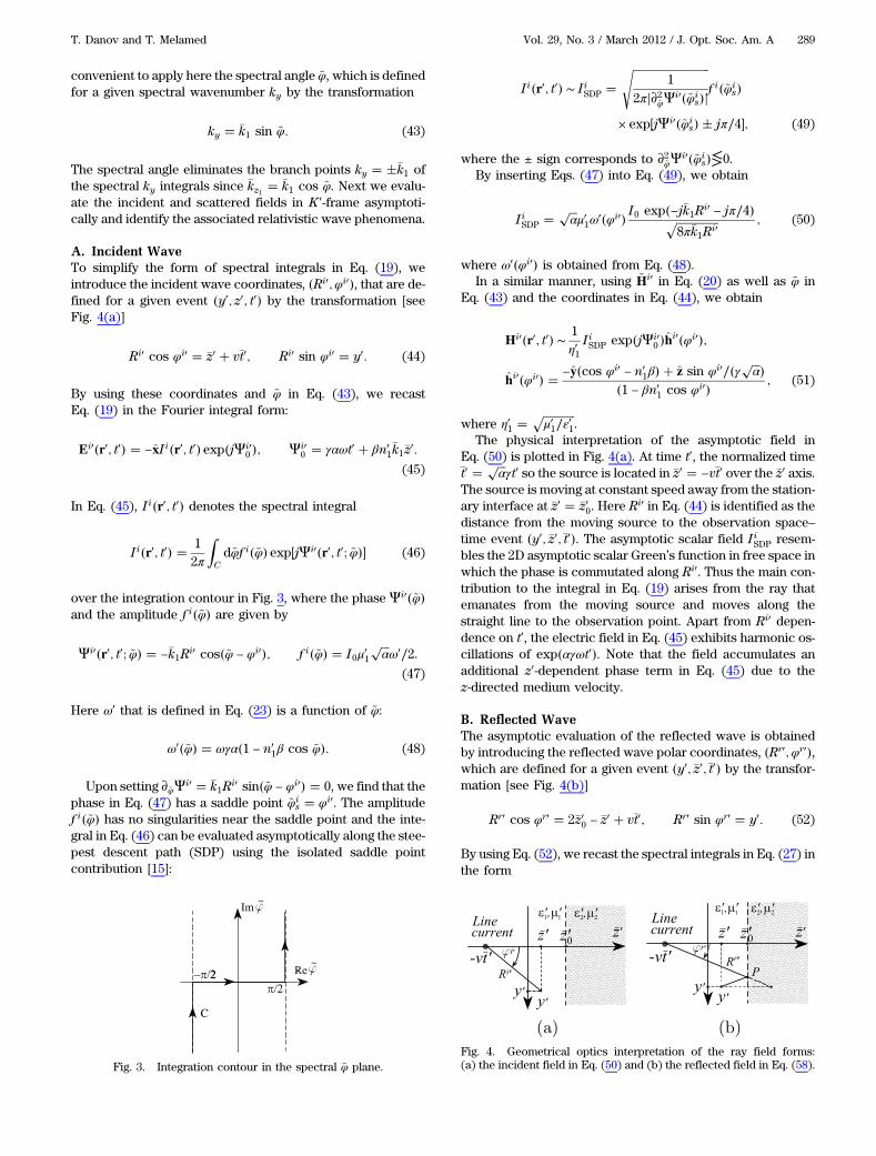
convenient to apply here the spectral angle ~φ, which is definedfor a given spectral wavenumber ky by the transformation

ky � �k1 sin ~φ: (43)

The spectral angle eliminates the branch points ky � ��k1 ofthe spectral ky integrals since �kz1 � �k1 cos ~φ. Next we evalu-ate the incident and scattered fields in K 0-frame asymptoti-cally and identify the associated relativistic wave phenomena.

A. Incident WaveTo simplify the form of spectral integrals in Eq. (19), weintroduce the incident wave coordinates, �Ri0;φi0�, that are de-fined for a given event �y0; z0; t0� by the transformation [seeFig. 4(a)]

Ri0 cos φi0 � �z0 � v�t0; Ri0 sin φi0 � y0: (44)

By using these coordinates and ~φ in Eq. (43), we recastEq. (19) in the Fourier integral form:

Ei0�r0; t0� � −xIi�r0; t0� exp�jΨi00 �; Ψi0

0 � γαωt0 � βn01�k1�z0:

(45)

In Eq. (45), Ii�r0; t0� denotes the spectral integral

Ii�r0; t0� � 12π

ZCd~φf i�~φ� exp�jΨi0�r0; t0; ~φ�� (46)

over the integration contour in Fig. 3, where the phase Ψi0�~φ�and the amplitude f i�~φ� are given by

Ψi0�r0; t0; ~φ� � −�k1Ri0 cos�~φ − φi0�; f i�~φ� � I0μ01��α

pω0∕2.

(47)

Here ω0 that is defined in Eq. (23) is a function of ~φ:

ω0�~φ� � ωγα�1 − n01β cos ~φ�: (48)

Upon setting ∂~φΨi0 � �k1Ri0 sin�~φ − φi0� � 0, we find that thephase in Eq. (47) has a saddle point ~φi

s � φi0. The amplitudef i�~φ� has no singularities near the saddle point and the inte-gral in Eq. (46) can be evaluated asymptotically along the stee-pest descent path (SDP) using the isolated saddle pointcontribution [15]:

Ii�r0; t0� ∼ IiSDP ��

12πj∂2~φΨi0�~φi

s�j

sf i�~φi

s�

× exp�jΨi0�~φis� � jπ∕4�; (49)

where the ± sign corresponds to ∂2~φΨi0�~φis�≶0.

By inserting Eqs. (47) into Eq. (49), we obtain

IiSDP � ��α

pμ01ω0�φi0� I0 exp�−j�k1Ri0 − jπ∕4��

8π�k1Ri0p ; (50)

where ω0�φi0� is obtained from Eq. (48).In a similar manner, using ~Hi0 in Eq. (20) as well as ~φ in

Eq. (43) and the coordinates in Eq. (44), we obtain

Hi0�r0; t0� ∼ 1η01

IiSDP exp�jΨi00 �hi0�φi0�;

hi0�φi0� � −y�cos φi0 − n01β� � z sin φi0∕�γ ��αp �

�1 − βn01 cos φi0� ; (51)

where η01 ��μ01∕ε01

p.

The physical interpretation of the asymptotic field inEq. (50) is plotted in Fig. 4(a). At time t0, the normalized time�t0 � ��αp γt0 so the source is located in �z0 � −v�t0 over the �z0 axis.The source is moving at constant speed away from the station-ary interface at �z0 � �z00. Here R

i0 in Eq. (44) is identified as thedistance from the moving source to the observation space–time event �y0; �z0;�t0�. The asymptotic scalar field IiSDP resem-bles the 2D asymptotic scalar Green’s function in free space inwhich the phase is commutated along Ri0. Thus the main con-tribution to the integral in Eq. (19) arises from the ray thatemanates from the moving source and moves along thestraight line to the observation point. Apart from Ri0 depen-dence on t0, the electric field in Eq. (45) exhibits harmonic os-cillations of exp�αγωt0�. Note that the field accumulates anadditional z0-dependent phase term in Eq. (45) due to thez-directed medium velocity.

B. Reflected WaveThe asymptotic evaluation of the reflected wave is obtainedby introducing the reflected wave polar coordinates, �Rr0;φr0�,which are defined for a given event �y0; �z0;�t0� by the transfor-mation [see Fig. 4(b)]

Rr0 cos φr0 � 2�z00 − �z0 � v�t0; Rr0 sin φr0 � y0: (52)

By using Eq. (52), we recast the spectral integrals in Eq. (27) inthe form

2

C

Fig. 3. Integration contour in the spectral ~φ plane.Fig. 4. Geometrical optics interpretation of the ray field forms:(a) the incident field in Eq. (50) and (b) the reflected field in Eq. (58).


Er0�r0; t0� � −xIr�r0; t0� exp�jΨr00 �;

Ψr00 � γαωt0 − βn0

1�k1��z0 − 2�z00�: (53)

In Eq. (53), Ir�r0; t0� denotes the spectral integral

Ir�r0; t0� � 12π

ZCd~φf r�~φ� exp�jΨr0�r0; t0; ~φ��; (54)

over the integration contour in Fig. 3 with

Ψr0�r0; t0; ~φ��−�k1Rr0 cos�~φ−φr0�; f r�~φ��Γ0�~φ�f i�~φ�; (55)

with f i�~φ� in Eq. (47). Γ0�~φ� denotes the reflection coefficient

Γ0�~φ��μ02�cos ~φ−n0

1β�−μ01��n0221�1−n0

1β cos ~φ�2−sin2 ~φ∕�αγ2�q

μ02�cos ~φ−n01β��μ01

��n0221�1−n0

1β cos ~φ�2−sin2 ~φ∕�αγ2�q ;

(56)

with n021 ≡ n0

2∕n01. The reflection coefficient has two branch

points that are denoted by ~φb1;2 . By setting the square rootin Eq. (56) to zero, we obtain in range ∣~φb1;2 ∣ ≤ π∕2

cos ~φb1;2 �n021n

02βαγ2 �

��n0

21n02βαγ2�2 − �n02

2 β2αγ2 � 1��n0221αγ2 − 1�

qn022 β2αγ2 � 1

: (57)

The branch points define two relativistic critical angles forwhich the spectral transferred PWs propagate parallel tothe interface [see Eq. (36)].

The integral in Eq. (54) has the stationary point ~φrs � φr0.

We distinguish two scattering regimes: under critical angle in-cidence in which ~φb1 < ~φr

s < ~φb2 and over critical angle inci-dence in which either ~φr

s < ~φb1 or ~φrs > ~φb2 .

1. Under Critical Angle IncidenceThe integration contour in this regime can be deformed intointegral along the SDP as plotted in Fig. 5(a). The reflectedwave is evaluated asymptotically by using the isolated saddlepoint contribution in (49). This procedure yields

Ir ∼ IrSDP � Γ0�φr0� ��α

pμ01ω0�φr0� I0 exp �−j�k1Rr0 − jπ∕4��

8π�k1Rr0p ; (58)

where, from Eq. (48), ω0�φr0� � ωγα�1 − βn01 cos φr0�. In a simi-

lar manner, by using ~Hr0 in Eq. (28) we obtain

Hr0�r0; t0� ∼ 1η01

IrSDP exp�jΨr00 �hr0�φr0�;

hr0�φr0� � y�cos φr0 − n01β� � z sin φr0∕�γ ��αp �

�1 − βn01 cos φr0� : (59)

The physical interpretation of the asymptotic EM field inEq. (58) is plotted in Fig. 4(b). The source, which is locatedin �z0 � −v�t0 over the �z0 axis, is moving at speed v away fromthe stationary interface. Here Rr0 in Eq. (52) is identified as thelength of the reflected ray from the interface to the observa-

tion space–time event �y0; �z0;�t0�. The ray path satisfies Snell’slaw in �y0; �z0� space (i.e., the angle of reflection equals the an-gle of incidence at time �t0).

2. Over Critical Angle IncidenceThe reflected field asymptotic evaluation for over critical an-gle incidence is preformed by deforming the integration pathof Ir in Eq. (54) to the integration contour in Fig. 5(b). Theelectric field is consist of two contributions

Er0�r0; t0� � Er0SDP�r0; t0� � Er0

b �r0; t0�; (60)

where Er0SDP denotes the contribution of the integration along

the SDP and E0b denotes the contribution of the integration

around the branch cut of ~φb1 (or ~φb2) in Eq. (57). The asymp-totic SDP contribution that arises from the vicinity of the sta-tionary point in the upper Riemann sheet is given in Eq. (53)with Eq. (58).

In the high-frequency regime, the main contribution to E0b

arises from points in the vicinity of the corresponding branchpoint in the upper Riemann sheet [16]. Therefore, in order toevaluate E0

b asymptotically, we apply a first-order Taylor ap-proximation to Γ0�~φ� in Eq. (56) about the branch point. Thus,for ~φ ≈ ~φb1;2 ,

Γ0�~φ�≃ 1� j2μ01

��2 sin ~φb1;2

p ��~φ − ~φb1;2

pγ ��αp ��

�cos ~φb1;2 − n01β��1 − n0

1β cos ~φb1;2 �q :

(61)

Equation (54) with Eq. (61) has the generic form of thebranch-cut integral [16]:

Ib �ZPb

d~φ�a� b

��~φ − ~φb

p �exp�Ωq�~φ��

∼b

��πp

�−Ωq0�~φb��3∕2exp�Ωq�~φb��; (62)

where Pb is a contour encircling the branch cut in the positivesense [see Fig. 5(b)], Ω is a large parameter, a and b are

Fig. 5. Integration contour in ~φ plane for the reflected field (a) underand (b) over critical angle incidence.


constants, q�~φ� is a regular in the vicinity of ~φb, and exp�Ωq�~φ��decays along the contour. Thus, by applying Eq. (62) toEq. (54) with Eqs. (57) and (61) for large real k1 values weobtain

Er0b �r0; t0� ∼ −xEr0

b1D0Er0

b2Er0b3 exp�jαγωt0�; (63)

where

Er0b1 �

I0��αp μ01ω0�φr��8π�k1L0

1

q exp�jΨ0b1�; (64)

with

Ψ0b1 � −�k1L0

1 − �π∕4� � βn01�k1�z00; L0

1 � ��z00 − v�t0�∕ cos θ0c:(65)

By comparing Eq. (64) to Eqs. (45) with (50), E0b1 is identified

as the incident ray that propagates from the source and im-pinges on the interface at the critical angle (angle of total re-flection) θ0c that is defined by

sin θ0c � n021 (66)

(see Fig. 6). The D0 term in Eq. (63), which is given by

D0 �2j sin2θ0c

��k1L0

1

q��αp γ�cos θ0c�3∕2

��cos θ0c − n0

1βp ��

1 − n01β cos θ0c

p ; (67)

is identified as the relativistic diffraction coefficient. The Er0b2

and Er0b3 terms in Eq. (63) are given by

Er0b2 �

exp�−j�k2L02�

��k2L02�3∕2

; L02 � y0 − L0

1 sin θ0c � ��z0 − �z00� tan θ0c;

(68)

where �k2 � ω��αϵ02μ02

p, and

Erb30 � exp�−j�k1L0

3� exp�jβn01�k1��z00 − �z0��;

L03 � ��z00 − �z0�∕ cos θ0c: (69)

The Er0b2 field term in Eq. (68) describes the relativistic lateral

ray that is propagating along L02 parallel to the interface in the

z0 � z0�0 medium. The lateral ray ��k2L02�−3∕2 decay along its tra-

jectory is due to the Erb30 field radiation back to n0

1 medium. Bycomparing Eqs. (53) with (58) to Eq. (69), the Er0

b3 field term isidentified as the ray that is propagating from the interface atangle θ0c to the observation point �y0; z0� along L0

3 (see Fig. 6).

Finally, by sampling the amplitude of ~Hr0 in Eq. (28) at ~φ �~φb1;2 and applying the same analytic procedure, we obtain theasymptotic head-wave magnetic field:

Hr0b �r0; t0� ∼

1η01

Er0b1D

0Er0b2E

r0b3 exp�jαγωt0�hr0�~φb1;2�;

hr0�~φb1;2� �y�cos ~φb1;2 − n0

1β� � z sin ~φb1;2∕�γ��αp �

�1 − βn01 cos ~φb1;2�

: (70)

C. Transmitted FieldThe exact transmitted EM field in K 0-frame is given by a spec-tral representation in Eq. (32). To simplify the form of thespectral integrals, we introduce the transmitted wave polarcoordinates, �Rt0

1 ; Rt02 ;φt0

1 ;φt02�, that are defined for a given

space–time event �y0; z0; t0� by the transformation (see Fig. 7)

Rt01 cos φt0

1 � �z00 � v�t0; Rt02 cos φt0

2 � �z0 − �z00; (71)

where angles φt01 and φt0

2 satisfy

tan φt02 �

�n021αγ2�−1 sin φt0

1 −n02�1−n0

1β cos φt01�β tan φt0

1��1−n0

1β cos φt01�2 − sin2φt0

1∕n0221αγ2

q : (72)

Equation (72) is identified later as the relativistic Snell’s law[see discussion following Eq. (83)]. Note that, by inverting thetransformation in Eq. (71), we obtain

y0 � Rt01 sin φt0

1 � Rt02 sin φt0

2 : (73)

By using Eq. (71) and the complex angle ~φ in Eq. (43), werecast the spectral integrals in Eq. (32) in the form

Et0�r0; t0� � −x exp�jΨi00 �r0; t0��It�r0; t0�;

It�r0; t0� � 12π

ZCd~φf t�~φ� exp�jΨt0�r0; t0; ~φ��; (74)

where Ψi00 is given in Eq. (45), the amplitude

f t�~φ� � T 0�~φ�f i�~φ�; (75)

with f i in Eq. (47), and the spectral phase Ψt0�~φ� is givenby

Fig. 6. Geometrical optics interpretation of the lateral (head) wavein Eq. (63).

Fig. 7. Geometrical optics interpretation of asymptotic transferredfield in Eq. (80).


Ψt0�r0; t0; ~φ� � −�k1

�Rt01 cos�~φ − φt0

1� � Rt02

�sin φt0

2 sin ~φ� n021 cos φt0

2

��1 − n0

1β cos ~φ�2 − sin2 ~φ∕n0221αγ2

q ��: (76)

The Fresnel transmission coefficient in the amplitude in Eq. (75) in terms of the spectral angle ~φ is given by

T 0�~φ� � 2μ02�cos ~φ − n01β�

μ02�cos ~φ − n01β� � μ01n0

21

��1 − n0

1β cos ~φ�2 − sin2 ~φ∕n0221αγ2

q : (77)

The stationary point that is denoted by ~φs1 is obtained bysetting ∂~φΨt0�~φ�j~φs1

� 0. By using Eqs. (71), (75), and (76), wefind that ~φs1 satisfies

y0 − tan ~φs1��z00 � v�t0� − tan ~φs2��z0 − �z00� � 0; (78)

where ~φs2 is related to ~φs1 by

tan ~φs2 ��n0

21αγ2�−1 sin ~φs1 − n02�1 − n0

1β cos ~φs1�β tan ~φs1��1 − n0

1β cos ~φs1�2 − sin2~φs1∕n0221αγ2

q :

(79)

By comparing Eqs. (78) and (79) with Eqs. (72) and (73), wededuce that ~φs1 � φt0

1 and, therefore, ~φs2 � φt02 .

By inserting Eqs. (78), (79) with (77) and (76), (75) into(49), we obtain the asymptotic expression of the transferredfield:

Et0�r0; t0� ∼ −xEt01E

t02 exp�jωγαt0�; (80)

where

Et01 � ��

αp

μ01ω0�φt01�I0 exp�−j�k1Rt0

1 � jβn01�k1�z00 − jπ∕4��

8π�k1Rt01

q (81)

and

Et02 � T 0�φt0

1� exp�−j�k2Rt02��

1� Rt02∕ρt0

p ; (82)

where T 0�φt01� is given in Eq. (77), and

ρt0 � Rt01

sin φt02 cos

2φt01

×�

n012�1−β2�n02

1 −n022 ��sin φt0

1 −n02β tan φt0

1

n012�1−β2�n0

12 −n0

22��−n0

2β∕cos3φt01 �n0

12 tan2φt0

2

�: (83)

Equation (78) sets the ray path that is shown in Fig. 7,where observation event �y0; �z0; t0� is represented by φt0

1 ,φt02 ; R

t01 ; R

t02 via Eq. (71). Following this definition, we identify

Eq. (78) as the path from the source along a straight line withangles ~φt

s1;2 � φt01;2 and lengths Rt0

1;2 in �z0 < �z00 or �z0 > �z00, re-spectively. Thus Eq. (79) [or Eq. (72)] describes the relativisticSnell’s law for this specific scattering scenario. This relationadjusts the angles to the source velocity. The spectral Doppler

shift in Eq. (23) changes the conventional (stationary) Snell’slaw, which is obtained for (K 0-frame) time-harmonic excita-tion. Note that, by setting β � 0 in Eq. (79), we obtainedthe well-known (stationary) Snell’s law.

The transferred field in Eq. (80) consists of Et01 in Eq. (81)

and Et02 in Eq. (82). By using Eq. (50) in Eq. (45), Et0

1 is identi-fied as the incident electric field at point P over the interface.This point is the intersection of the incident ray, which is ema-nating from the source with departure angle φt0

1 and the inter-face at �z0 � �z0 0. Thus, Rt0

1 is identified as the radius ofcurvature of the incident wavefront at point P (see Fig. 7).The second term in the transferred field, Et0

2 , is identified asthe ray field that is propagating in �z0 > �z0 0 medium alongthe optical path Rt0

1 . By using Eq. (83), we identify ρt0 as theprincipal radius of curvature of the transferred wavefrontat point P.

The corresponding magnetic transferred field is obtainedfrom Eq. (33), giving

Ht0�r0; t0� ∼ 1η02

Et01E

t02 exp�jωγαt0�ht0�φi0�;

ht0�φi0� �−y cos φt0

2 � z sin φt01∕

�n021γ

��αp ��1 − n0

1β cos φt01�

: (84)

5. ASYMPTOTIC FIELDS IN K-FRAMEA. Incident FieldThe asymptotic fields in K 0-frame are transformed to K -frameby applying the inverse field transformation of Eq. (4) and ILTEq. (2) to Eqs. (45), (50), and (51) with K 0-frame constitutiverelations in Eq. (7). This results in

Ei�r; t� ∼ −xEix�r� exp�jωt�;

Eix�r� � I0ωμ01α1∕2

exp �−j�k1Ri − jπ∕4��8π�k1Ri

p exp�jkmz�;

Hi�r; t� ∼ 1η01

Eix�r� exp�jωt�

�−y cos φi � z

��α

psin φi

�; (85)

where Ri ��y2 � �z2

pand cos φi � �z∕Ri. These expressions

are used later for identifying the incident ray field contributionto the reflected and transmitted fields.

B. Reflected FieldIn Subsection 4.B we distinguished two reflection regimes inwhich the K 0-frame incident ray is impinging on the interface


with an angle that is larger or smaller than the critical angle. Inthis subsection, we identify the K -frame relativistic wave phe-nomena associated with these two scattering regimes.

1. Under Critical Angle IncidenceThe under critical angle scattering regime for which in K 0-frame ~φb1 < ~φr

s < ~φb2 was investigated in Subsection 4.B.1.By applying ILT we obtained that, in K -frame, the stationarypoint is given by

~φrs � cos−1

� γ2 ��αp �2�z0 � vt� − z�1� β2��y2 � γ4α�2�z0 � vt� − z�1� β2��2

p �. (86)

By inserting Eqs. (53) and (59) with Eq. (58) into Eq. (7) andthen into the field transformation in Eq. (4) and using ILT inEq. (2), we obtain the reflected field (isolated saddle pointcontribution) in K -frame in the form

Er�r; t� ∼ −xErx�r; t� exp�jΨr�; (87)

where

Ψr � γ2α�1� β2n021 �ωt − βγ2

��α

p�k1�z�1� n02

1 �∕n01 − 2n0

1z0�;

Erx�r; t� � ωμ01γ2α3∕2Γ�φr�

I0 exp�−j�k1Rr − j π4

��8π�k1Rr

p ; (88)

with

Rr ��y2 � γ4α�2�z0 � vt� − z�1� β2��2

q;

cos φr � γ2��α

p �2�z0 � vt� − z�1� β2��∕Rr;

Γ�φr� � �1 − 2βn01 cos φr � β2n02

1 �Γ0�φr�. (89)

Γ0 is given in Eq. (56).In a similar manner,

Hr�r; t� ∼ 1η01

Erx exp�jΨr�hr�φr�;

hr�φr� � y�cos φr�1� β2n021 � − 2βn0

1� � z sin φr∕γ2 ��αp

1 − 2βn01 cos φr � β2n02

1

: (90)

2. Over Critical Angle IncidenceThe over critical angle scattering regime for which, inK 0-frame, ~φr

s < ~φb1 or ~φrs > ~φb1 was investigated in

Subsection 4.B.2. ~φrs in K -frame is given in Eq. (86). Following

the discussion preceding Eq. (60), the reflected electric fieldconsists of two contributions

Er�r; t� � ErSDP�r; t� � Er

b�r; t�; (91)

where ErSDP denotes the contribution of the integration along

the SDP, which is given in Eq. (87), and Eb denotes the con-tribution of the integration around the branch cut of ~φb1 (or~φb2) in Eq. (57). Following the K 0-frame representation inEq. (63), we define

L1 ��α

pγ2�z0 � β2z − vt�∕ cos θ0c;

L3 ��α

pγ2�z0 − z� vt�∕ cos θ0c;

L2 � Rr sin φr − L1 sin θ0c ��α

pγ2�z − z0 − vt� tan θ0c: (92)

By inserting Eqs. (63) and (70) into Eq. (7) and then into thefield transformation in Eq. (4) and using ILT in Eq. (2), weobtain

Erb�r; t� ∼ −xEr

b1DErb2E

rb3 exp �jαγ2ω�t − βz∕c��; (93)

where

Erb1�

I0γ2α3∕2μ01ω�φr��8π�k1L1

p �1−2βn01 cosφr�β2n02

1 �exp�jΨb1�; (94)

with

Ψb1 � −�k1L1 − π∕4� βn01�k1

��α

pγ2z0: (95)

By comparing Eq. (64) to Eqs. (45) with (50), Erb1is identified

as the incident ray that propagates from the source and im-pinges on the interface at the critical angle θ0c in Eq. (66).The D term in Eq. (93), which is given by

D � 2j sin θ0c��k1L1

p��αp γ�cos θ0c�3∕2

��cos θ0c − n0

1βp ��

1 − n01β cos θ0c

p ; (96)

is identified as the relativistic diffraction coefficient. The Erb2

and Erb3 terms in Eq. (93) are given by

Erb2�

exp�−j�k2L2��k2L2�3∕2

; (97)

Erb3� exp�−j�k1L3� exp�jβn0

1�k1

��α

pγ2�z0 − z� vt��: (98)

C. Transferred FieldBy applying the field transformation to Eq. (80), we obtain theasymptotic refracted fields in K -frame:

Etx�r; t� ∼ −xEt

1�r; t�Et2�r; t� exp�jαγ2ω�t − βz∕c��; (99)

where

Et1 � I0μ01γ2α3∕2ω�φt

1�exp�−j�k1Rt

1 � j�k1n01β

��αp γ2z0 − jπ∕4��8π�k1Rt

1

q ;

Et2 �

T�φt1� exp�−j�k2Rt

2��1� Rt

2∕ρtp ; (100)

with T�φt1� � T 0�1 − n0

1β cos φt1 � n0

2β cos φt2�. T 0 is given in

Eq. (77), and

cos φt1 �

��α

pγ2�z0 � vt − β2z�∕Rt

1;

cos φt2 �

��α

pγ2�z − z0 − vt�∕Rt

2; (101)


Rt1 �

��y2P � αγ4�z0 � vt − β2z�2

q;

Rt2 �

��y − yP�2 � αγ4�z − z0 − vt�2

q; (102)

where yP � Rt01 sin φt0

1 denotes the y-axis value of the intersec-tion point P of the incident ray and the interface (see Fig. 7).

6. CONCLUSIONSIn this paper we have investigated the canonical problem ofthe 2D longitudinal Green’s function of a uniformly moving(lossless and dispersion-free) dielectric–magnetic mediumwith a planar discontinuity. The exact solution in the formof PW spectral integrals, as well as asymptotic solutions, wereobtained in both the laboratory frame and the comovingframe. Interpretation of the relativistic asymptotic solutionsin the form of ray fields was given. New canonical ray formswere derived for the relativistic incident fields, reflectedfields, lateral wave, and transmitted (refracted) fields. This re-search and future investigations can eventually lead to estab-lishing a relativistic geometrical theory of diffraction.

REFERENCES1. C. Tai, “The dyadic Green’s function for a moving isotropic

medium,” IEEE Trans. Antennas Propag. 13, 322–323 (1965).2. J. V. Bladel, Relativity and Engineering (Springer, 1984).3. T. Mackay and A. Lakhtakia, “Negative phase velocity in a uni-

formly moving, homogeneous, isotropic, dielectric-magneticmedium,” J. Phys. A 37, 5697–5711 (2004).

4. T. Mackay, A. Lakhtakia, and S. Setiawan, “Positive-, negative-,and orthogonal-phase-velocity propagation of electromagneticplane waves in a simply moving medium,” Optik 118, 195–202(2007).

5. A. Lakhtakia and W. Weiglhofer, “On electromagnetic fields in alinear medium with gyrotropic-like magnetoelectric properties,”Microwave Opt. Technol. Lett. 15, 168–170 (1997).

6. A. Lakhtakia and T. Mackay, “Simple derivation of dyadic Greenfunctions of a simply moving, isotropic, dielectric-magneticmedium,” Microwave Opt. Technol. Lett. 48, 1073–1074 (2006).

7. M. Idemen and A. Alkumru, “Relativistic scattering of a plane-wave by a uniformly moving half-plane,” IEEE Trans. AntennasPropag. 54, 3429–3440 (2006).

8. P. De Cupis, G. Gerosa, and G. Schettini, “Gaussian beam dif-fraction by uniformly moving targets,” Atti della FondazioneGiorgio Ronchi 56, 799–811 (2001).

9. P. D. Cupis, “Radiation by a moving wire-antenna in the pre-sence of plane interface,” J. Electromagn. Waves Appl. 14,1119–1132 (2000).

10. W. Arrighetti, P. De Cupis, and G. Gerosa, “Electromagneticradiation from moving fractal sources: A plane-wave spectralapproach,” Prog. Electromagn. Res. 58, 1–19 (2006).

11. P. D. Cupis, “Electromagnetic wave scattering from movingsurfaces with high-amplitude corrugated pattern,” J. Opt. Soc.Am. A 23, 2538–2550 (2006).

12. T. Danov and T. Melamed, “Spectral analysis of relativistic dya-dic Green’s function of a moving dielectric-magnetic medium,”IEEE Trans. Antennas Propag. 59, 2973–2979 (2011).

13. J. Kong, Theory of Electromagnetic Waves (Wiley, 1975).14. M. Idemen and A. Alkumru, “Influence of motion on the edge-

diffraction,” Prog. Electromagn. Res. B 6, 153–168 (2008).15. L. Felsen and N. Marcuvitz, Radiation and Scattering of Waves

(IEEE, 1994), Chap. 4.2.16. L. Felsen and N. Marcuvitz, Radiation and Scattering of Waves

(IEEE, 1994), Chap. 4.8.


two-dimensional relativistic longitudinal green s function ...timormel/index_files/linecurrent...

Documents