Two-Dimensional Non-Hermitian Fermion Systems

A Thesis

Presented to

The Division of Mathematics and Natural Sciences

Reed College

In Partial Fulfillment

of the Requirements for the Degree

Bachelor of Arts

Connor J. Wallace

May 2013

Approved for the Division(Physics)

Katherine Jones-Smith

Acknowledgements

I owe most my progress at Reed to the excellent professors I’ve had across all dis-ciplines. Two professors outside of my major in particular, Elizabeth Drumm andKen Brashier have been instrumental to my development as a student. Within thephysics department, I give my heartfelt thanks to Lucas Illing, Joel Franklin, andNelia Mann, for teaching me how to work hard and enjoy it too. I would also like toacknowledge Johnny Powell for being a source of support and a helpful voice through-out my college career. To my thesis advisor, Kate, I owe you a very special thanks.Not only did you readily share your PhD. work to help produce this document, youwould always drop what you were doing when I came looking for help. You alwaysencouraged me to create a thesis that I found exciting, from my own thoughts and ofmy own volition. I am so grateful to you, and to the fates for having sent me such awonderful advisor. Last, I would like to acknowledge my office mates Noah Muldavin,Lukas Kuczynski, and Maxwell Gurewitz. Thanks for being my friends, I could nothave hoped for more interesting, fun or nicer people in my life over these few years.

Preface

The goal of this thesis is to reexamine the quantum Hall effect from the perspectiveof non-hermitian quantum mechanics to see what changes might occur to the compu-tation. This document examines the behavior of two-dimensionally-confined fermionssubject to a normal magnetic field without interactions, impurities, or other-such dif-ficulties. While the title describes this thesis as pertaining to fermions in a magneticfield, the only fermion-ness we require is for charged, massive particles that do notoccupy the same state.

For at least half a century, conventional quantum mechanics textbooks have tacitlyassumed that only hermitian operators (operators equal to their conjugate transpose)may pertain to observables[1][2]. Hermitian observables arise when imposing the self-adjointness of operators over an orthonormal basis, and so they would naturally arisein any practical calculation. The basic point of non-hermitian theories is that aself-adjoint observable operating over a non-normalized basis is not necessarily Dirachermitian[3], despite being physically relevant.

One of the nicest properties of hermitian operators is that they are guaranteed

to have real eigenvalues, and hence the values of observables would automatically beall-real if all observables were hermitian. However, there are whole classes of non-hermitian operators which may have spectra that are all real, or real for a range ofvalues of non-hermitian parameters. Furthermore, an increasing number of physicalsystems exhibiting non-hermitian behaviors continue to arise, which theories like PT-quantum mechanics are able to predict with excellent accuracy. Where are systemshermitian, why does a system digress into a non-hermitian regime, and what arethe characteristics of a non-hermitian system? By exploring non-hermitian quantummechanics, we hope that the role of hermiticity will be better understood in additionto perhaps uncovering new physics.

While exploring the depth of this topic, I had hopes to extend my reach intospin-dynamics and the deeper instances of the Hall effect (such as the fractionalquantum Hall effect, or spin-momentum locking in topologically non-trivial states ofmatter). It turns out that describing the dynamics of PT-quantum mechanics even fora straightforward system can be challenging, and so I was forced to limit myself. As itstands, the quantum Hall effect serves as a very basic case from which to springboardinto non-hermitian quantum theory, specifically PT-quantum mechanics. In fact, Iformulate the simplest toy model I could physically motivate to perturb with a non-hermitian term. The introduction serves to acquaint the reader with the brief, basic,pseudo-quantitative explanation of the behavior of the qHe according to conventional

quantum theory. We re-derive some of the more famous results, such as the Landaulevels and energy quantization, and leave out the subtleties. The paper is then free tointroduce and explain Non-Hermitian Quantum Mechanics and within the Hall effectand jump into PT-quantum mechanics.

Table of Contents

Introduction . . . . . . . . . . . . . . . . . . . . . . . . . . . . . . . . . . . 1

0.1 The Hall Effect . . . . . . . . . . . . . . . . . . . . . . . . . . . . . . 10.2 PT-Quantum Mechanics . . . . . . . . . . . . . . . . . . . . . . . . . 5

Chapter 1: Modeling a fermion in a magnetic field . . . . . . . . . . . 9

1.1 Classical Motion . . . . . . . . . . . . . . . . . . . . . . . . . . . . . 91.2 Quantum Mechanics . . . . . . . . . . . . . . . . . . . . . . . . . . . 121.3 Square Lattice . . . . . . . . . . . . . . . . . . . . . . . . . . . . . . . 15

Chapter 2: The Non-Hermitian Hamiltonian . . . . . . . . . . . . . . . 19

2.1 Theory . . . . . . . . . . . . . . . . . . . . . . . . . . . . . . . . . . . 192.1.1 PT-Quantum Mechanics . . . . . . . . . . . . . . . . . . . . . 192.1.2 PT-Phase Transition . . . . . . . . . . . . . . . . . . . . . . . 20

Chapter 3: Momentum Perturbation . . . . . . . . . . . . . . . . . . . . 23

Chapter 4: Computation . . . . . . . . . . . . . . . . . . . . . . . . . . . . 29

4.1 Energy Eigenvalues . . . . . . . . . . . . . . . . . . . . . . . . . . . . 29

Chapter 5: Results . . . . . . . . . . . . . . . . . . . . . . . . . . . . . . . 33

5.0.1 Analytic Eigenfunctions . . . . . . . . . . . . . . . . . . . . . 335.0.2 Hofstadter Butterflies . . . . . . . . . . . . . . . . . . . . . . . 345.0.3 Real vs. imaginary Eigenvalues . . . . . . . . . . . . . . . . . 37

Conclusion . . . . . . . . . . . . . . . . . . . . . . . . . . . . . . . . . . . . . 45

Appendix A: Derivations . . . . . . . . . . . . . . . . . . . . . . . . . . . . 47

A.0.4 Hermite Polynomials . . . . . . . . . . . . . . . . . . . . . . . 47A.0.5 Longitudinal Current[4] . . . . . . . . . . . . . . . . . . . . . 51

References . . . . . . . . . . . . . . . . . . . . . . . . . . . . . . . . . . . . . 53

List of Figures

1 A charged particle confined to a plane is deflected in a normal magneticfield . . . . . . . . . . . . . . . . . . . . . . . . . . . . . . . . . . . . 2

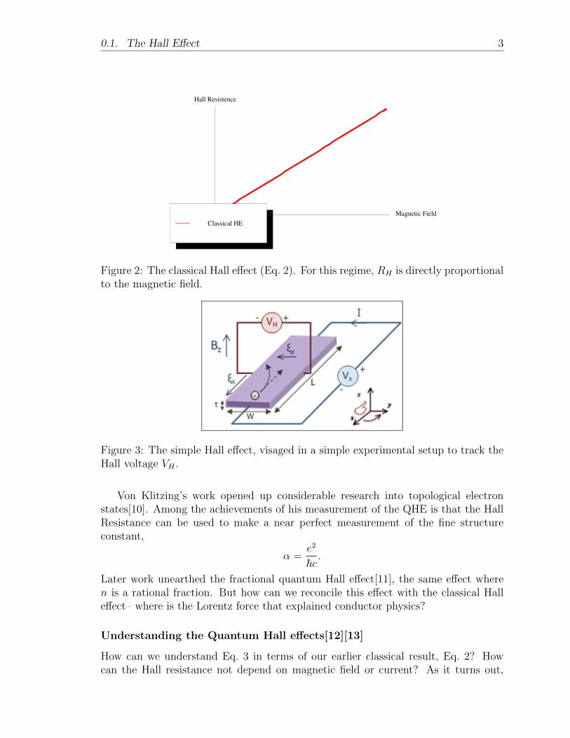
2 The classical Hall effect (Eq. 2). For this regime, RH is directly pro-portional to the magnetic field. . . . . . . . . . . . . . . . . . . . . . 3

3 The simple Hall effect, visaged in a simple experimental setup to trackthe Hall voltage VH . . . . . . . . . . . . . . . . . . . . . . . . . . . . 3

4 The quantum Hall effect. pxy (RH) is quantized and pxx (the resistancealong the current) is 0. As the magnetic field increases, the Hall resis-tance increases as a step function and pxx experiences spikes at the lipof the step[5]. . . . . . . . . . . . . . . . . . . . . . . . . . . . . . . . 4

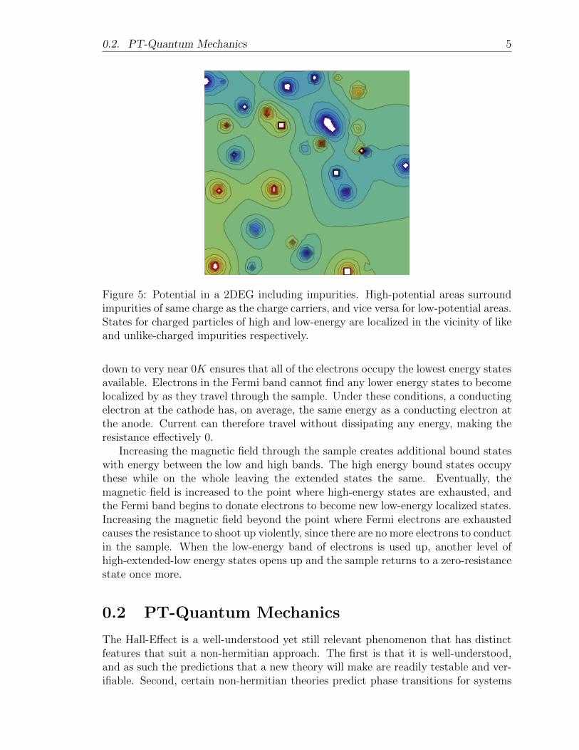
5 Potential in a 2DEG including impurities. High-potential areas sur-round impurities of same charge as the charge carriers, and vice versafor low-potential areas. States for charged particles of high and low-energy are localized in the vicinity of like and unlike-charged impuritiesrespectively. . . . . . . . . . . . . . . . . . . . . . . . . . . . . . . . . 5

6 The band structure for electrons confined to a two dimensional layerwith an applied magnetic field, including charged impurities. The blueband represents high energy states (H), green are low energy states(L), and red, extended states (Ex). Whitespace in the band structureindicates available space in a given band. As the perpendicular Bfield increases, the high energy band within the highest Landau levelempties into low energy states. . . . . . . . . . . . . . . . . . . . . . . 6

1.1 Classical motion for an electron in a strong magnetic field. The particleorbits at a fixed radius, and is localized. . . . . . . . . . . . . . . . . 10

1.2 Classical motion for a particle in an electromagnetic field where E andB are perpendicular to each other. Notice that the net displacementof the particle is parallel with the electric field. . . . . . . . . . . . . . 10

1.3 Classical motion for an electron in an electromagnetic field where E

and B are perpendicular to each other, and E is strong compared withB. . . . . . . . . . . . . . . . . . . . . . . . . . . . . . . . . . . . . . 10

1.4 The real (red) and imaginary (blue) parts of the n = 1, k=2π/L wavefunction Ψ1[x, y]. Here l is set to 1 for simplicity . . . . . . . . . . . . 14

1.5 The eigenvalue spectrum for Harper’s equation with α[0, 1], called theHofstadter butterfly[6]. The vertical axis varies α, while the horizontalaxis indicates (which in this case shows the interval [−4, 4]). . . . . 17

2.1 Coupled LRC circuit exhibiting PT-phase transition according to Eq. 2.10.(Bittner et al., Phys Rev. Lett 108, 2 024101 (2012)) . . . . . . . . . 21

3.1 The “Hamiltonian” matrix for the Bloch energy formulation of theNelson-Hatano system on a 5-site, continuous lattice. . . . . . . . . . 25

3.2 The unperturbed “Hamiltonian” matrix for the Bloch energy formula-tion of the Nelson-Hatano system on a 5-site, continuous lattice. . . . 25

3.3 The perturbation “Hamiltonian” matrix for the Bloch energy formula-tion of the Nelson-Hatano system on a 5-site, continuous lattice. . . . 25

3.4 Im[] (vertical axis) vs. Re[] (horizontal axis) for n = 1000, g = 0.4 inthe Nelson and Hatano system[7]. The red line indicates the eigenvaluespectrum for Eq. 3.10., while the black indicates the exact formulationfrom their original publication (Eq. 3.4.). The red line spectrum isblurred and opaque to show the correspondence between the two spectra. 26

3.5 The 3x3 Hamiltonian describing the perturbed Harper’s equation fora three site lattice in Eq. 3.22. . . . . . . . . . . . . . . . . . . . . . . 27

4.1 Two mathematica scripts used to find eigenvalues and manipulate data.The script “newnnh” creates the n× n perturbed Hamiltonian matrixcorresponding to the perturbed harper’s equation on a continuous n-site lattice. “hofstadter” creates the Hamiltonian matrix for the groundcase (where there is no non-hermitian term). . . . . . . . . . . . . . . 30

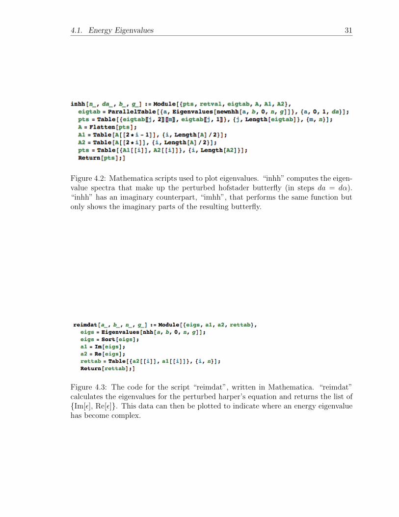
4.2 Mathematica scripts used to plot eigenvalues. “inhh” computes theeigenvalue spectra that make up the perturbed hofstader butterfly (insteps da = dα). “inhh” has an imaginary counterpart, “imhh”, thatperforms the same function but only shows the imaginary parts of theresulting butterfly. . . . . . . . . . . . . . . . . . . . . . . . . . . . . 31

4.3 The code for the script “reimdat”, written in Mathematica. “reim-dat” calculates the eigenvalues for the perturbed harper’s equationand returns the list of Im[], Re[]. This data can then be plotted toindicate where an energy eigenvalue has become complex. . . . . . . 31

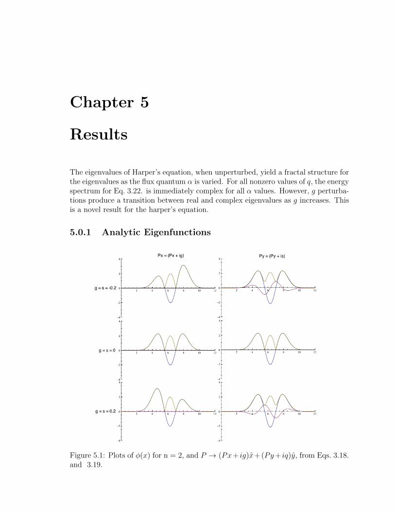
5.1 Plots of φ(x) for n = 2, and P → (Px + ig)x + (Py + iq)y, fromEqs. 3.18. and 3.19. . . . . . . . . . . . . . . . . . . . . . . . . . . . 33

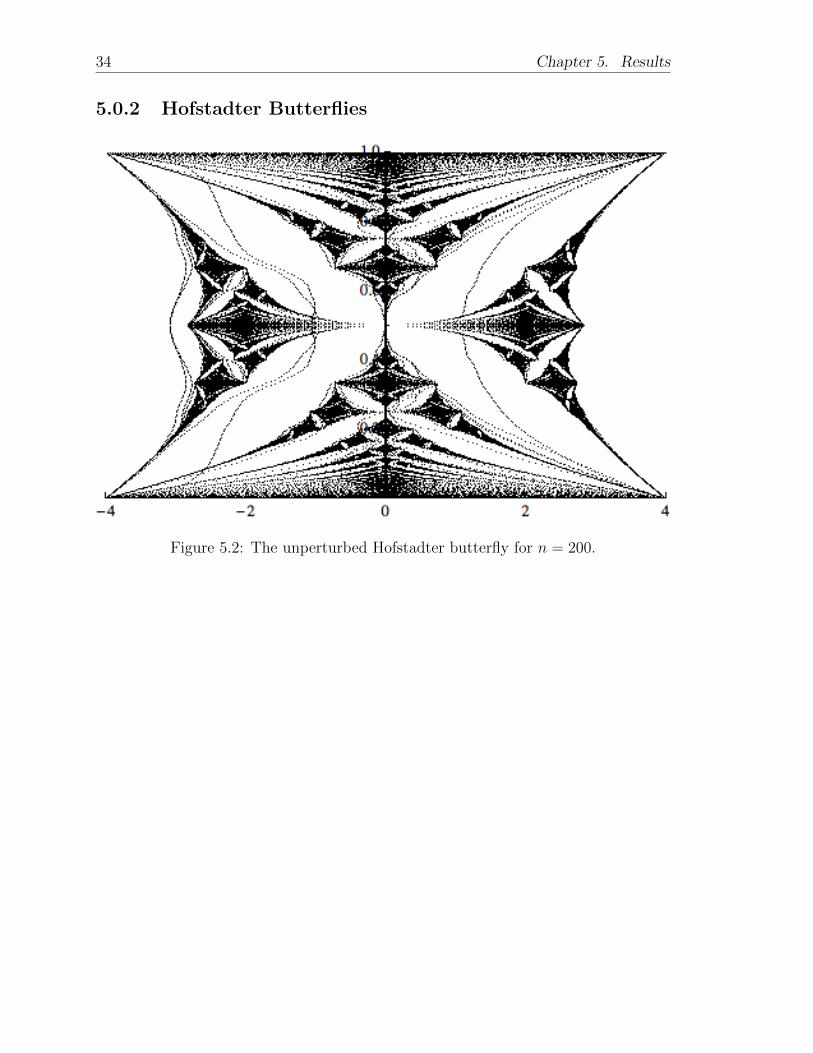
5.2 The unperturbed Hofstadter butterfly for n = 200. . . . . . . . . . . . 345.3 The real spectra of the perturbed Hofstadter butterfly for n = 200,

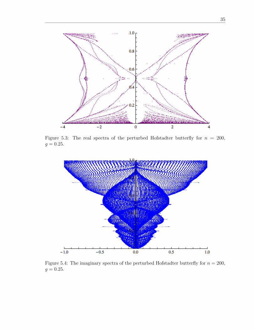
g = 0.25. . . . . . . . . . . . . . . . . . . . . . . . . . . . . . . . . . . 355.4 The imaginary spectra of the perturbed Hofstadter butterfly for n =

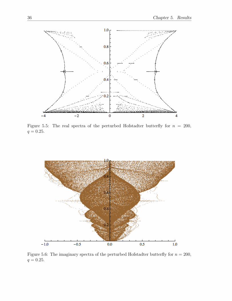
200, g = 0.25. . . . . . . . . . . . . . . . . . . . . . . . . . . . . . . . 355.5 The real spectra of the perturbed Hofstadter butterfly for n = 200,

q = 0.25. . . . . . . . . . . . . . . . . . . . . . . . . . . . . . . . . . . 365.6 The imaginary spectra of the perturbed Hofstadter butterfly for n =

200, q = 0.25. . . . . . . . . . . . . . . . . . . . . . . . . . . . . . . . 365.7 Real vs. imaginary eigenvalue plots for α = 0.2 on a 1000-site lattice.

Blue pertains to g (x) perturbation and orange to q (y) perturbation 37

5.8 Real vs. imaginary eigenvalue plots for α = 0.411 on a 1000-site lattice.Blue pertains to g (x) perturbation and orange to q (y) perturbation 38

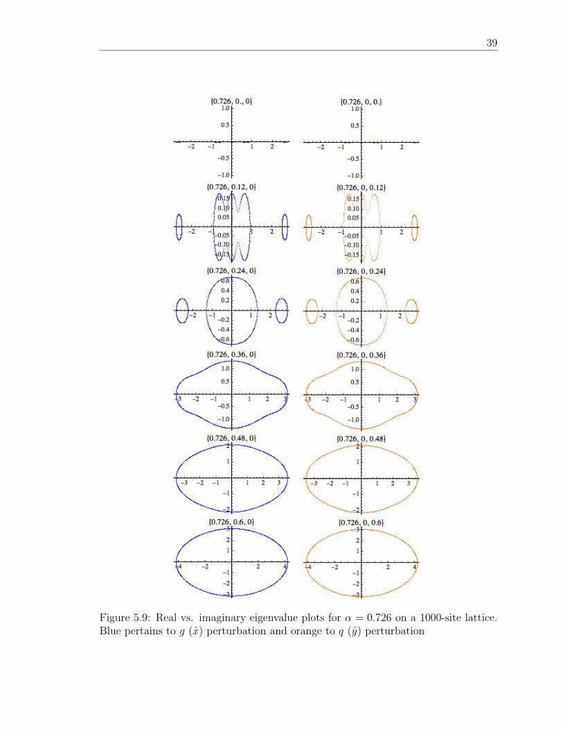
5.9 Real vs. imaginary eigenvalue plots for α = 0.726 on a 1000-site lattice.Blue pertains to g (x) perturbation and orange to q (y) perturbation 39

5.10 Real vs. imaginary eigenvalue plots for α = 0.8 on a 1000-site lattice.Blue pertains to g (x) perturbation and orange to q (y) perturbation. 40

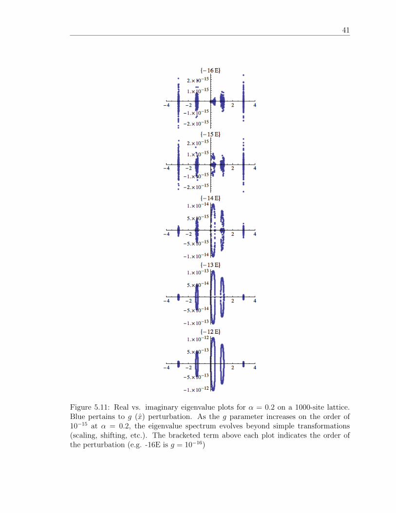
5.11 Real vs. imaginary eigenvalue plots for α = 0.2 on a 1000-site lattice.Blue pertains to g (x) perturbation. As the g parameter increases onthe order of 10−15 at α = 0.2, the eigenvalue spectrum evolves beyondsimple transformations (scaling, shifting, etc.). The bracketed termabove each plot indicates the order of the perturbation (e.g. -16E isg = 10−16) . . . . . . . . . . . . . . . . . . . . . . . . . . . . . . . . . 41

5.12 Real vs. imaginary eigenvalue plots for α = 0.4 on a 1000-site lat-tice. Blue pertains to g (x) perturbation. A move from all-real tocomplex eigenvalues appears while varying g on the order of 10−15 atα = 0.4. The bracketed term above each plot indicates the order ofthe perturbation (e.g. -16E is g = 10−16) . . . . . . . . . . . . . . . . 42

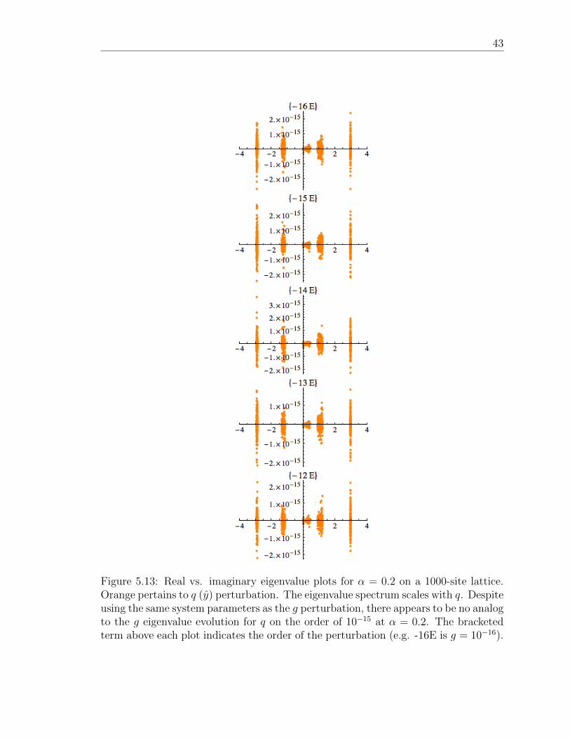
5.13 Real vs. imaginary eigenvalue plots for α = 0.2 on a 1000-site lattice.Orange pertains to q (y) perturbation. The eigenvalue spectrum scaleswith q. Despite using the same system parameters as the g perturba-tion, there appears to be no analog to the g eigenvalue evolution for qon the order of 10−15 at α = 0.2. The bracketed term above each plotindicates the order of the perturbation (e.g. -16E is g = 10−16). . . . 43

5.14 Real vs. imaginary eigenvalue plots for α = 0.4 on a 1000-site lattice.Orange pertains to q (y) perturbation. There appears to be no analogto the g eigenvalue evolution for q on the order of 10−15 at α = 0.4.The eigenvalue spectrum simply scales with q. The bracketed termabove each plot indicates the order of the perturbation (e.g. -16E isg = 10−16). . . . . . . . . . . . . . . . . . . . . . . . . . . . . . . . . . 44

Abstract

This paper considers the physics of the Hall effect beginning from elementary prin-ciples, leading to a non-hermitian perturbation of several quantum Hall toy models.Beginning with the history of the Hall effect, the physics of fermions in a magneticfield is introduced, outlined, and derived. This treatment yields intuition, a grasp ofthe problem, and a simple, conventional model of a fermion in a magnetic field ona two-dimensional lattice. The precepts of PT-quantum mechanics are then laid outand a non-hermitian Hamiltonian is constructed using a complex momentum pertur-bation. Finally, results are obtained that suggest a PT-phase transition within theBloch square lattice model, a novel result for the quantum Hall Hamiltonian.

Dedication

For my mom, my dad, and my brother.

Introduction

Behavior of Fermions in a Magnetic Field

The theory of fermion behavior in a magnetic field is one of the crown jewels ofcontemporary theoretical physics. Quantum mechanics has predicted a plethora ofsurprising phenomena decades ahead of experimental confirmations, providing com-pelling support for conventional quantum theories. Despite these victories, fermionbehavior is still one of the most hotly researched topics in physics. Physicists havediscovered that fermion behavior is a problem of vast scope. The most importantmilestones in fermion theory, far from closing off avenues, have begged more ques-tions than they’ve answered while revealing phenomena beyond the human intuition.

What follows is a qualitative overview of the major phenomena associated withfermions in a strong magnetic field. These explanations contextualize the phenomenareferred to in this thesis in a relatable way.

0.1 The Hall Effect

The Hall effect is a well-understood phenomenon that occurs in a current-carryingmaterial subjected to a magnetic field. The phenomenon is totally split into itstwo regimes– the classical and the quantum mechanical– with each describing vastlydifferent behavior. The classical Hall effect was first discovered in 1879 by EdwinHall[8]. A full century after the Hall effect was discovered, a hitherto unknown andpronounced behavior called the quantum Hall effect was observed in the laboratory byKlaus Von Klitzing[9]. The seemingly simple and straightforward Hall effect, his papershowed, is not only non-linear, but it also can exhibit incredible quantum effects. Ina conductor, charge carriers such as negative electrons or positive charge “holes” arefree to move. When a voltage is applied across such a conductor, the charge carriersare forced through the sample, creating current. Classically, a charged particle movingin the presence of a magnetic field experiences a force according to the Lorentz forcelaw,

F = e( E + v × B), (1)

where e is the charge of a particle, v is the velocity vector of the particle and B isthe magnetic field vector.

Within a thin conducting layer, charged particles move tangent to the magnetic

2 Introduction

Figure 1: A charged particle confined to a plane is deflected in a normal magneticfield

field at all times where the magnetic field is normal to the surface. With a constantelectric field across the surface, positive charges are forced in one direction and neg-ative charges are forced in the opposite direction. According to the Lorentz forcelaw, holes and electrons moving according to the same electric field are forced in thesame direction by the same magnetic field. Creating a current moving perpendicularto the magnetic field causes positive and negative charge carriers to be forced apartperpendicular to both E and B, creating a potential. The induced voltage perpen-dicular to both the electric and magnetic fields is called the Hall Voltage, VH . Theproportionality between voltage, current and magnetic field is a parameter called theHall resistance RH [10],

RH =VH

I=

Bz

eD, (2)

where e is the charge of the current carrier and D is their density per unit area.RH changes linearly with B, as we might expect. This linear relation between Hallresistance is exactly what researchers confirmed for nearly a century, before highenergy magnetic fields and extremely low temperatures were attainable in the lab.

In 1980, under extreme magnetic fields and close to absolute zero, Klaus VonKlitzing observed RH behaving like a “staircase function” of B, changing abruptly tosome small changes and staying constant for huge changes. His data hinted that RH

is not directly related to the magnetic field. Instead it is given by integer values [9],

RH =h

ne2. (3)

The Hall resistance is an integer fraction multiple of /e2: no direct dependenceon B or I. The Von Klitzing constant,

RK = RH1 = RK = 25, 812.807Ω,

being made of fundamental constants, is one of the most precise constants inphysics[9]. Von Klitzing’s results show a remarkable coincidence between Hall resis-tance plateaus and a perpendicular state of 0 resistivity (see Fig.4.). When the Hallresistance is a constant, the resistance perpendicular to the Hall voltage (the currentcarrying direction) is 0. The zero resistivity state can therefore be switched on andoff with relatively small changes in the magnetic field.

0.1. The Hall Effect 3

Magnetic Field

Hall Resistence

Classical HE

Figure 2: The classical Hall effect (Eq. 2). For this regime, RH is directly proportionalto the magnetic field.

Figure 3: The simple Hall effect, visaged in a simple experimental setup to track theHall voltage VH .

Von Klitzing’s work opened up considerable research into topological electronstates[10]. Among the achievements of his measurement of the QHE is that the HallResistance can be used to make a near perfect measurement of the fine structureconstant,

α =e2

c.

Later work unearthed the fractional quantum Hall effect[11], the same effect wheren is a rational fraction. But how can we reconcile this effect with the classical Halleffect– where is the Lorentz force that explained conductor physics?

Understanding the Quantum Hall effects[12][13]

How can we understand Eq. 3 in terms of our earlier classical result, Eq. 2? Howcan the Hall resistance not depend on magnetic field or current? As it turns out,

4 Introduction

Figure 4: The quantum Hall effect. pxy (RH) is quantized and pxx (the resistancealong the current) is 0. As the magnetic field increases, the Hall resistance increasesas a step function and pxx experiences spikes at the lip of the step[5].

Hall quantization has no classical explanation: we require quantum mechanics toprovide a mathematical proof. Before deriving it explicitly, a semiclassical, qualitativeexplanation of the quantum Hall phenomenon follows.

To begin, consider the model of a two-dimensional electron gas, as shown inFig. 0.1, including some impurities. According to the Pauli exclusion principle, notwo fermions occupy the same state. In a low temperature environment, electronstend to have filled the lowest available states. Wave functions, as we will see later,come in highly degenerate groups called Landau levels– large sets of available statesthat have the same energy (theoretically speaking). In real life where samples haveimpurities, Landau levels contain a slim range of energies that a fermion like an elec-tron can occupy. As we will see, the disorder of the system is, in a bizarre twist, thefeature of the system that lead to Von Klitzing’s famous observations of macroscopicorder.

Within a Landau level, there are low-energy bound states, high-energy boundstates, and extended states. For electrons, the low-energy states occur near an im-purity of a positive charge, and the high-energy states are localized near impuritiesof positive charge. Both low and high-energy states are localized in the sample whileextended states can move about. The band of mobile electrons in extended states aregrouped into what is called the Fermi band, a group of similar energy electron statesthat have higher energy than the low-energy localized states and the Fermi energy,but lower energy than high-energy localized states. Electrons supplied from the cath-ode travel through the conductor, and when they encounter a free low-energy statethey prefer to occupy it and give off energy in the form of heat. Cooling the system

0.2. PT-Quantum Mechanics 5

Figure 5: Potential in a 2DEG including impurities. High-potential areas surroundimpurities of same charge as the charge carriers, and vice versa for low-potential areas.States for charged particles of high and low-energy are localized in the vicinity of likeand unlike-charged impurities respectively.

down to very near 0K ensures that all of the electrons occupy the lowest energy statesavailable. Electrons in the Fermi band cannot find any lower energy states to becomelocalized by as they travel through the sample. Under these conditions, a conductingelectron at the cathode has, on average, the same energy as a conducting electron atthe anode. Current can therefore travel without dissipating any energy, making theresistance effectively 0.

Increasing the magnetic field through the sample creates additional bound stateswith energy between the low and high bands. The high energy bound states occupythese while on the whole leaving the extended states the same. Eventually, themagnetic field is increased to the point where high-energy states are exhausted, andthe Fermi band begins to donate electrons to become new low-energy localized states.Increasing the magnetic field beyond the point where Fermi electrons are exhaustedcauses the resistance to shoot up violently, since there are no more electrons to conductin the sample. When the low-energy band of electrons is used up, another level ofhigh-extended-low energy states opens up and the sample returns to a zero-resistancestate once more.

0.2 PT-Quantum Mechanics

The Hall-Effect is a well-understood yet still relevant phenomenon that has distinctfeatures that suit a non-hermitian approach. The first is that it is well-understood,and as such the predictions that a new theory will make are readily testable and ver-ifiable. Second, certain non-hermitian theories predict phase transitions for systems

6 Introduction

Figure 6: The band structure for electrons confined to a two dimensional layer withan applied magnetic field, including charged impurities. The blue band representshigh energy states (H), green are low energy states (L), and red, extended states(Ex). Whitespace in the band structure indicates available space in a given band. Asthe perpendicular B field increases, the high energy band within the highest Landaulevel empties into low energy states.

with non-hermitian terms. Given that the hallmark (pun intended) of the effect is aseries of phase transitions within the system makes the quantum Hall effect a greatcandidate system. Third, there are explanations utilizing Parity and Time-reversalquantum mechanics (PT-quantum mechanics or PTQM) to shed light on high tem-perature superconductivity and quantum magnetism[14]. As such, it ought to predictsimpler phenomena, and may perhaps shed new light into the behavior of a seeminglywell-understood problem (a point that Von Klitzing can surely relate to).

PT-quantum mechanics is a formulation of quantum mechanics that allows forcertain non-hermitian operators to pertain to physical observables. This works byworking over non-orthonormal bases (non-normalized bases). Holding operators tobe self-adjoint enforces different rules according to the specific definition of the innerproduct. Over an orthonormal basis for φ of some vectors,

n|m = δn,m,

0.2. PT-Quantum Mechanics 7

making the wave function φ,

|φ =N

i=1

an|n. (4)

For a self-adjoint operator A,

Aφ|ψ = φ|Aψ, (5)

with φ, ψ orthonormal implies that A = (A∗)T . Choosing other bases for φ andrequiring an operator A be self-adjoint implies a different set of criteria on A[15],and these do not restrict physical operators to be strictly equal to their conjugatetranspose. PTQM has developed the theory into a self-consistent and reliable the-ory that has already predicted various unique phenomena. One of the major fieldsin which PTQM has made consistent predictions is within in the field of quantumoptics, where Hamiltonian terms such as complex potentials pop up often. For suchsystems, PTQM has predicted numerous experimental results to an excellent degreeof accuracy.

Chapter 1

Modeling a fermion in a magnetic

field

1.1 Classical Motion

To understand how charged particles behave within a non-hermitian framework, weneed a model to work on and to build a base case with which to compare the eventualresults. We will begin by creating a classical picture of a particle traveling in thex − y plane in a magnetic field. This classical model also yields an intuition abouthow our particles should behave under normal conditions.

According to the Lorentz force law, a classical particle experiences a force F ,

F = e( E + v × B). (1.1)

⇒ F = e [(yBz − zBy) x+ (zBx − xBz) y + (xBy − yBx) z] + E.

Since B = ∇ × A, where A is the magnetic vector potential, we find the x-component of the force as,

Fx = e

y

∂Ay

∂x− ∂Ax

∂y

− z

∂Ax

∂z− ∂Az

∂x

+ Ex = mx. (1.2)

To simplify the force expression, assume a perpendicular magnetic field Bz z, andthat our electric field points in the y direction. According to Newton’s second law,

F = ma ⇒ mx = −eBzy, my = eBzx+ eEy. (1.3)

Solving Eq. 1.3 where E → 0 yields the parametrization of a circle,

x[t] = A cos[eBt/m+ δ], y[t] = A sin[eBt/m+ δ]. (1.4)

This is what we might expect for a particle moving in the presence of a strongmagnetic field: it orbits at some radius A. Solving this equation for finite electricfields produces non-localized circles– orbits combined with linear motion, as shownin Figs. 1.1., 1.2. and 1.3.

10 Chapter 1. Modeling a fermion in a magnetic field

Figure 1.1: Classical motion for an electron in a strong magnetic field. The particleorbits at a fixed radius, and is localized.

Figure 1.2: Classical motion for a particle in an electromagnetic field where E and B

are perpendicular to each other. Notice that the net displacement of the particle isparallel with the electric field.

Figure 1.3: Classical motion for an electron in an electromagnetic field where E andB are perpendicular to each other, and E is strong compared with B.

We see that electrons can occupy a localized “orbit” and also travel relativelyunhindered by the magnetic field, all depending on the relative field strengths.

The Lagrangian

The Lagrangian provides a bridge between classical and quantum regimes. The La-grangian, L, is defined as

L = T − V

where T represents the kinetic energy and V represents some potential. For a particlein a magnetic field, the Lagrangian is

L = 1/2mv2 − e(φ+ v · A), (1.5)

In the Quantum Hall regime, the electric field term φ is very small compared with A,and we can remove it, leaving the effective Lagrangian

L = 1/2mv2 − ev · A. (1.6)

1.1. Classical Motion 11

Before we continue, let’s make sure that this system will reproduce the behavior thatwe found with the Lorentz force. The Euler-Lagrange equations are conditions thatminimize the path that the particle may take given some conditions, yielding theequations of motion for such paths. The Euler-Lagrange equations say

∂L

∂α=

d

dt

∂L

∂α. (1.7)

For the x-component we have

mx− e∂Ax

dt= −e

x∂Ax

∂x+ y

∂Ax

∂y+ z

∂Ax

∂z

,

⇒ mx = e

dAx

dt− x

∂Ax

∂x− y

∂Ax

∂y− z

∂Ax

∂z

.

By the chain rule

dAx

dt=

d

dtAx =

∂

∂x

dx

dt+

∂

∂y

dy

dt+

∂

∂z

dz

dt

Ax. (1.8)

This leaves,

mx = e

y

∂Ay

∂x− ∂Ax

∂y

− z

∂Ax

∂z− ∂Az

∂x

(1.9)

as in Eq. 1.2, confirming that our Lagrangian describes motion for the x-componentaccording to the Lorentz force law and vice versa.

The Hamiltonian

We can use the Lagrangian to develop the Hamiltonian, a more useful tool in quantummechanics. It is defined from the Lagrangian as follows:

H =

piqi − L. (1.10)

With L ≈ 12mx

2 − e(v · A), Eq. 1.7 yields the velocity in terms of mechanicalmomentum,

∂L

∂xµ= p

µ = mxµ − eA

µ → xµ =

pµ + eA

µ

m

. (1.11)

Finally, the Hamiltonian can be written,

H =1

2m(p+ eA)2. (1.12)

To study particles confined to a plane with a magnetic field normal to it, thevector potential should be vastly simplified. In the next step, choose the Landaugauge

A → −Bxy

12 Chapter 1. Modeling a fermion in a magnetic field

called the Landau gauge. It confines the magnetic field to the z direction. TheHamiltonian now becomes,

H =1

2m(pxx+ pyy − eBxy)2 =

1

2m(p2

x+ p

2y− 2pyeBx+ e

2B

2x2),

H =1

2m[p2

x+ (py − eBx)2]. (1.13)

1.2 Quantum Mechanics

Up until now, the treatment has been entirely classical. The form of Eq. 1.13 allowsfor an easy transition between classical and quantum regimes. While in the classicalcase, the momenta were themselves parameters, in quantum mechanics the momenta,and the Hamiltonian itself is treated as an operator. The momentum parameterbecomes the operator,

P = i∇. (1.14)

For the momentum in a single cartesian direction, the momentum operator is,

px =i

∂

∂x. (1.15)

According to the Schrodinger equation,

HΨ = EΨ. (1.16)

The eigenvalues of the operator H acting on a wavefunction Ψ are some set ofdefinite energies E. The energy spectrum is the set of energies that a particle withwavefunction Ψ can be measured to have. From Eq. 1.13, we can see that the formof our governing equation is simple in y, but not x. In this case, it makes sense tosuggest the ansatz for the wave functions. Assume that the particle wave functionsare plane waves along our y-axis, Ψk(x, y) → φk(x)eiky. One of the benefits of thissubstitution is clear when we find the eigenvalues of py,

py[Ψ] = pkΨ,

i

∂

∂y

eikyyφ(x)

= pke

ikyyφ(x)

⇒ pk = ky. (1.17)

We can substitute this into our Hamiltonian to make it one-dimensional for someconstant parameter ky, a great bonus. From Eq. 1.13,

1

2mp2xφ(x) +

1

2m(ky − eBx)2φ(x) = Eφ(x). (1.18)

Now, define the magnetic length

l =

eB

1.2. Quantum Mechanics 13

, and the cyclotron frequencyωc = eB/m

. Plugging these in yields

1

2mp2xφ(x) +

1

2mω

2c(x− kl

2)2φ(x) = Eφ(x). (1.19)

Converting the momentum to its operator form in Eq. 1.15. reduces the Hamiltonianto differential equation in x, k,

− 22m

∂2φ

∂x2+

1

2mω

2c(x− kl

2)2φ(x) = Enφ(x). (1.20)

To create a neat graph of the wave functions, it helps to non-dimensionalizeEq. 1.20. To solve this equation analytically, define a useful dimension x

as,

lx = x− kl

2. (1.21)

Note that x is a non-dimensional variable. Plugging our relevant parameters intothe equation yields,

− 22ml2

∂2φ

∂x2 +1

2mω

2c(lx)2φ(x) = Enφ(x),

−ωc

2

∂2φ

∂x2 +ωc

2(x)2φ(x) = Enφ(x

).

Making the nifty non-dimensionalization E = E0, and choosing E0 = ωc sim-plifies the expression to,

−1

2

∂2φ

∂x2 +x2

2φ(x) = φ(x). (1.22)

Using this method yields a class of n solutions with the accompanying conditionon the energy of the system:

φn(x) = AHn(x

)e−x2/2, n = (n+ 1/2), (1.23)

where Hn(x) is the nth Hermite polynomial, and the normalization constant A isfound to be (See Appendix A),

A =1√

2nn!π1/2. (1.24)

Replacing x for x from Eq. 1.21. yields

φn(x) =1√

2nn!π1/2Hn(x− kl

2)e−(x−kl2)2/2l2 (1.25)

φn(x, y) =1√

2nn!π1/2eiky−(x−kl

2)2/2l2Hn(x− kl

2). (1.26)

14 Chapter 1. Modeling a fermion in a magnetic field

Figure 1.4: The real (red) and imaginary (blue) parts of the n = 1, k=2π/L wavefunction Ψ1[x, y]. Here l is set to 1 for simplicity

If the y-axis has periodic boundaries, then we know that kP → 2πP/L, where P isan integer. n is called the Landau level– a highly degenerate grouping of states thathave the same energy. A plot of the wave function from Eq. 1.26 shown in Fig 1.2.

Before continuing from this picture, take note of the dimensionalized energy eigen-values,

En = E0n = ωc(n+ 1/2). (1.27)

The energy levels are quantized, defining the allowed energy that a particle canbe measured to have. Further, these energy levels depend on the cyclotron frequencyωc, which is proportional to the magnetic field. As we increase the magnetic field, weexpect the energy of each level to increase. Changing the magnetic field also changesthe magnetic length and therefore the wave functions too. Note that the increase ofE0 is a B-dependent parameter, while l is also B-dependent. To get Hall quantization,we need a new parameter that describes the system in terms of its Landau levels.

The Filling Factor:(ν)

Assuming that particles are evenly distributed within the sample, how many particlesexist in a given Landau level? As is clear from the form of Eq. 1.26., the centers ofbounded states are shifted in x. The wave function for given k, l values is centered ata value of x such that

x− kl2 = 0. (1.28)

Imposing periodic boundary conditions on the y direction of the wave function en-forces a condition for state spacing in the x-direction. For such a condition we find

eiky(y+Ly) = e

ikyy (1.29)

1.3. Square Lattice 15

implying

ky =2πP

Ly

. (1.30)

Now consider some length Lx in x. Within this length there are N states, and Eq. 1.28gives

Lx =2πNl

2

Ly

⇒ N =LxLy

2πl2. (1.31)

The number of states per unit area (degeneracy per unit area) comes readily fromthis equation,

D =N

LxLy

=1

2πl2. (1.32)

We can now define the filling factor ν, the number of particles in a Landau level, interms of the particle density ρ:

ν =ρ

D= 2πl2ρ. (1.33)

For the nth Landau level, the current density J(r) is

J(r) = −neρ(r)v(r), (1.34)

eventually leading to the longitudinal current (See Appendix A.0.2).

Iy = −ne

dpy

2π

∂H

∂py

(1.35)

Iy = −ne

h

∂E

∂x(1.36)

Iy =ne

2

hVH (1.37)

Finally retrieving Eq. 3., the Hall resistance for n filled Landau levels is,

RH =VH

Iy=

h

ne2. (1.38)

1.3 Square Lattice

We can extend the analytic system to a discrete lattice. For a square lattice withspacing a, the tight-binding model yields the Bloch energy function[6],

W (k) = 2E0(cos(kxa) + cos(kya)). (1.39)

We make the famous Peirels substitution,

k = p− e A, (1.40)

16 Chapter 1. Modeling a fermion in a magnetic field

⇒ ky =py − eAy

, kx =px

. (1.41)

Plugging this in to the Bloch energy function gives

W (k) = E0((eiapx + e

− iapx ) + (e

iapy − ieBxa

+ e− iapy

+ ieBxa )). (1.42)

Eq. 1.42 contains the canonical translation operators,

T (+a) = eia p,

T (−a) = e− ia

p.

These operators, when acting on a wave function, shift the wave function by alattice position like so,

T (+a)Ψ(β) = Ψ(β + a). (1.43)

The equation thus becomes,

W (k) = E0

T (+ax) + T (−ax) + e

− ieBax T (+ay) + e

ieBax T (−ay)

. (1.44)

Whose eigenvalues are then given by,

E0(Ψ(x+ a, y) +Ψ(x− a, y) + e− ieBax

Ψ(x, y + a)

+ eieBax

Ψ(x, y − a)) = EΨ(x, y). (1.45)

The form of Eq. 1.45 allows us to capture both B and l dependence at the same time.To this end, define a new parameter α,

α =a2

2πl2=

a2eB

2π . (1.46)

In this case, α will be the stand-in for magnetic field strength as it defines the strengthof the magnetic field relative to the size of the lattice. We can see that as it incor-porates Eq. 1.32 and the lattice size, it is also the number of wave functions in eachlattice square. As we saw in Eq. 1.26, the wave functions and energy levels shoulddepend on the magnetic field and the size of our system to the magnetic field. Theparameter α combines the two into a single parameter.

On a lattice, x = ma and y = na for some integers m,n > 0. To modelplane-waves in the y-direction, we have the square lattice equivalent to the ansatz inEq. 1.17,

Ψ(ma, na) = φ(m)eiηm.

When plugged in,

eiηn

φ(m+ 1) + φ(m− 1) + (e−2imπα+iη + e

2imπα−iη)φ(m)= e

iηnφ(m),

1.3. Square Lattice 17

Finally yielding “Harper’s equation”,

φ(m+ 1) + φ(m− 1) + 2 cos[2mπα− η]φ(m) = φ(m). (1.47)

To calculate for lattices of interesting size, we use a computer. We are interestedin how the set of changes as we vary our parameter α.The very intricate structureof as α is varied is shown in Fig. 1.5.

Figure 1.5: The eigenvalue spectrum for Harper’s equation with α[0, 1], called theHofstadter butterfly[6]. The vertical axis varies α, while the horizontal axis indicates (which in this case shows the interval [−4, 4]).

Chapter 2

The Non-Hermitian Hamiltonian

2.1 Theory

An operator A is hermitian if it is equal to its own conjugate transpose,

A = (A∗)T = A†. (2.1)

The inner product of two hermitian states Ψ and Φ is,

< Ψ|Φ >= Ψ†Φ = (Ψ∗)TΦ. (2.2)

The eigenvalues of are the possible results of measurement[1],and hermitian oper-ators are guaranteed to have real eigenvalues. Furthermore, hermitian operators giverise to unitary time evolution,

|Ψ(t) = e−iHt/|Ψ0. (2.3)

Unitarity guarantees that the norm of a wave function be invariant under time evo-lution (also known as probability conservation).

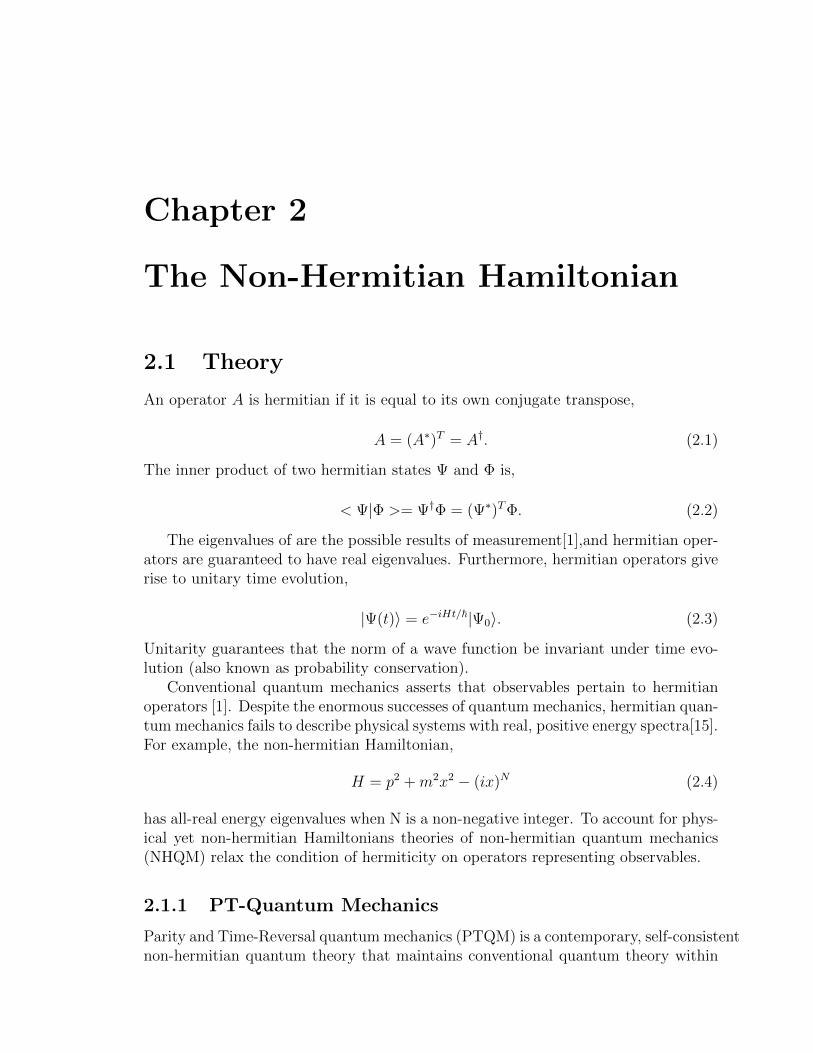
Conventional quantum mechanics asserts that observables pertain to hermitianoperators [1]. Despite the enormous successes of quantum mechanics, hermitian quan-tum mechanics fails to describe physical systems with real, positive energy spectra[15].For example, the non-hermitian Hamiltonian,

H = p2 +m

2x2 − (ix)N (2.4)

has all-real energy eigenvalues when N is a non-negative integer. To account for phys-ical yet non-hermitian Hamiltonians theories of non-hermitian quantum mechanics(NHQM) relax the condition of hermiticity on operators representing observables.

2.1.1 PT-Quantum Mechanics

Parity and Time-Reversal quantummechanics (PTQM) is a contemporary, self-consistentnon-hermitian quantum theory that maintains conventional quantum theory within

20 Chapter 2. The Non-Hermitian Hamiltonian

a less-restrictive framework. PTQM systems exhibit strange and unexpected proper-ties, and it has predicted several striking physical phenomena, most notably a novelphase transition in non-hermitian systems.

Instead of imposing hermiticity on operators, PTQM reverts to the less restrictivecondition that operators be self-adjoint with respect to the inner product. Since aself-adjoint inner product is hermitian when evaluated over an orthonormal basis,evaluating over an orthogonal basis allows certain non-hermitian operators to pertainto observables. We can represent the action of the Parity operator with a matrix S:PΨ = SΨ, and the action of the Time-reversal operator with complex conjugation,TΨ = Ψ∗. As such, PTQM can use the Parity and Time operators themselves toenforce the condition of a self-adjoint inner product space,

(Ψ|Φ) ≡ (PTΨ)TΦ = Ψ†SΦ = Ψ†

PΦ. (2.5)

Quantum theories are typically formulated over orthonormal bases where eachunit vector is perpendicular to the other and has length 1. For two such basis vectorsfi, fj, their inner product is,

fi|fj = δij. (2.6)

In PTQM, the same calculation becomes

(fi|fj) = k[x]δij. (2.7)

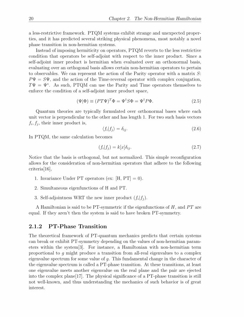
Notice that the basis is orthogonal, but not normalized. This simple reconfigurationallows for the consideration of non-hermitian operators that adhere to the followingcriteria[16],

1. Invariance Under PT operators (ex: [H, PT] = 0).

2. Simultaneous eigenfunctions of H and PT.

3. Self-adjointness WRT the new inner product (fi|fj).

A Hamiltonian is said to be PT-symmetric if the eigenfunctions of H, and PT areequal. If they aren’t then the system is said to have broken PT-symmetry.

2.1.2 PT-Phase Transition

The theoretical framework of PT-quantum mechanics predicts that certain systemscan break or exhibit PT-symmetry depending on the values of non-hermitian param-eters within the system[3]. For instance, a Hamiltonian with non-hermitian termproportional to g might produce a transition from all-real eigenvalues to a complexeigenvalue spectrum for some value of g. This fundamental change in the character ofthe eigenvalue spectrum is called a PT-phase transition. At these transitions, at leastone eigenvalue meets another eigenvalue on the real plane and the pair are ejectedinto the complex plane[17]. The physical significance of a PT-phase transition is stillnot well-known, and thus understanding the mechanics of such behavior is of greatinterest.

2.1. Theory 21

Figure 2.1: Coupled LRC circuit exhibiting PT-phase transition according to Eq. 2.10.(Bittner et al., Phys Rev. Lett 108, 2 024101 (2012))

Consider the non-hermitian Hamiltonian matrix describing a system made of bothan energy source and an energy well coupled together by constant g (see [18] for anin-depth description). Solving the Schrodinger equation for this system yields theequations,

aeiθψ1 + gψ2 = ψ1 (2.8)

gψ1 + ae−iθ

ψ2 = ψ2 (2.9)

The matrix representation of these equations yields the Hamiltonian

H =

ae

iθg

g ae−iθ

. (2.10)

The reality of the spectrum of H depends on the coupling constant, g. For g2<

a2 sin2(θ), the eigenvalues of H are complex, and the system is said to be in a broken

PT phase. However, for g2 > a2 sin2(θ), the eigenvalues of H are all real, and H is said

to be in an unbroken PT phase. At g2 = a

2 sin2(θ) the system transitions betweenPT-symmetric and broken PT-symmetry regions, called a PT-phase transition.

Characteristics of PT-phase transitions

Eq. 2.10. is a theoretical description of at least three separate physical systems.Schindler et al. implemented an LRC-equivalent coupled pair of LRC circuits[19].Bittner et al. reconstructed an equivalent optical system of the Hamiltonian withcoupled lossy and pumped waveguides and a microwave cavity[17]. After these exper-iments, Bender constructed a simple coupled pendulum system offering an accessibleexample of a PT-phase transition[18]. Each of these experiments has reproduced thetheorized PT-phase transition to an excellent degree of accuracy.

These simple systems commensurate with Eq. 2.10. display several commonal-ities. Each system describes a coupled system where energy is exchanged betweenoscillators. The coupling term determines the stability of the solution. For certainregimes of the coupling term, the system is forced into or out of energetic equilibrium(breaking PT-symmetry). When the system breaks PT symmetry, the system runsoff in a pair of negative and positive gain states, similar to a diverging wave function.

Chapter 3

Momentum Perturbation

PT-quantummechanics allows us to consider an entirely new category of Hamiltoniansthat differ significantly with hermitian theories. Adding complex perturbations to theHamiltonian will take our system into the regions where hermitian theories do notreach, while keeping a clear base case. Perturbing the hermitian Hamiltonian H

should yield a non-hermitian perturbation Hamiltonian Hi:

H → H0 + βHi. (3.1)

For reasons that will become clear, I propose to make the following momentum per-turbation motivated by the results of Nelson and Hatano[7],

P → P + iβ. (3.2)

Adding a complex constant to the momentum has a few different physical interpre-tations. The complex perturbation could come about through moving through somesmall complex vector field[20], for instance. Although thoroughly non-hermitian,this change produces real energy spectra for a range of parameters in similar latticeHamiltonians.

The edit is simple, it produces a PT-phase transition in some system, and as wewill discover, the Nelson-Hatano system is very similar in form to the resulting non-hermitian Harper’s equation (Eq. 3.22). What follows is a summary of the relevantresults of Nelson and Hatano’s studies of a particle on a one-dimensional lattice witha random potential[7][20][21].

A Non-Hermitian Hamiltonian with a Random Potential

The Hamiltonian for a particle in a single-dimension with both a random potentialand the perturbation from Eq 3.2. is

H =(Px + ig)2

2m+ V (x). (3.3)

While Nelson and Hatano provide a lattice version of this Hamiltonian,

Hx,x = − t

2

egδx,x+1 + e

−gδx,x−1

+ Vxδx,x , (3.4)

24 Chapter 3. Momentum Perturbation

this lattice Hamiltonian is not derived in an equivalent way to the Harper Hamilto-nian. To stay consistent, we are motivated to reformulate this Hamiltonian accordingto the Bloch energy theorem method used by Hofstadter. As before, the Bloch energytheorem forces the energy function W (kx) to have the form,

W (kx) = 2E0 cos[kxa] + E0V (x). (3.5)

Making the same identifications in Eqs. 1.40. and 1.41. yields the familiar form forthe energy,

W (kx) = E0

eiPxa + e

−iPxa+ V (x). (3.6)

Finding the energy eigenvalues and non-dimensionalizing yields,

eiPxa Ψ(x) + e

−iPxa Ψ(x)

+ V (x)Ψ(x) = Ψ(x). (3.7)

Making the non-hermitian transition Px → Px + ig yields,

e− ga

eiPxa Ψ(x) + e

ga e

−iPxa Ψ(x)

+ V (x)Ψ(x) = Ψ(x). (3.8)

There are two important things to note: first, the leading exponential terms con-taining g can be simplified by absorbing the common factor into a new constant g

leaving the non-dimensionalized exponent,

ega = e

g, (3.9)

As we will see later, producing the perturbed Hofstadter butterfly requires non-dimensionalizing g to retrieve a non-trivial factor. Since a and and g do not relate tothe system in any overarching way, we can get by without non-dimensionalizing sinceg is just a constant. Further, this eigensystem (Eq. 3.8) includes the same canonicaltranslation operators as introduced in Eq. 1.43. Replacing these and noting x = ma,we get,

e−gφ(m+ 1) + e

gφ(m− 1) + V (m)φ(m) = φ(m). (3.10)

Now examine the form of Eq. 3.10. in relation to Eq. 3.4. For t = 2, V (m) =Vx/a in the range [−1, 1] (the exact system parameters from [7]), these treatmentsare simply negatives of each other and should therefore yield a reversed eigenvaluespectrum.

Note that the Nelson-Hatano system can be broken into the form of Eq. 3.1 bydefining,

H0 = Ψ(m+ 1) +Ψ(m− 1) + V (m)Ψ(m), (3.11)

and,

βHi =e−g − 1

Ψ(m+ 1) + [eg − 1]Ψ(m− 1)

. (3.12)

25

H5 =

∈[-1,1] e−g 0. 0. e

g

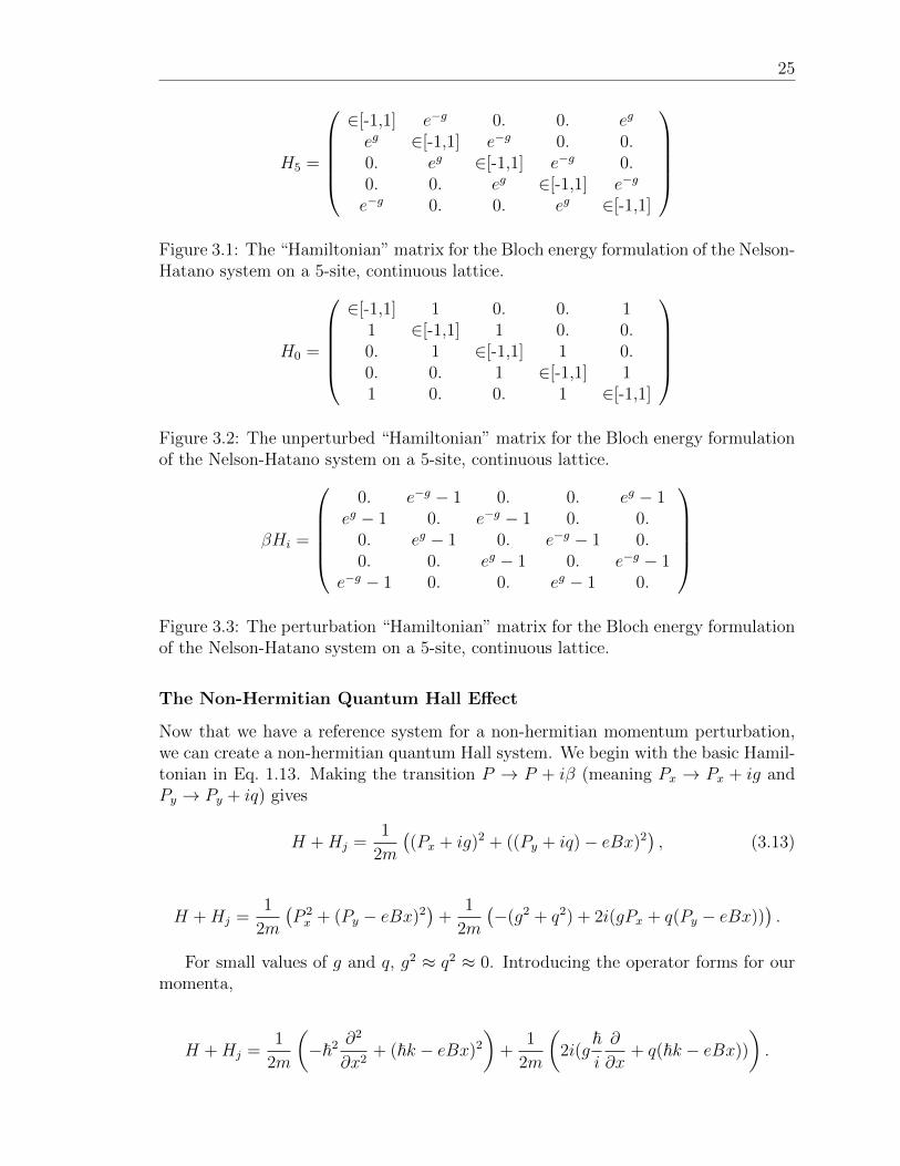
eg ∈[-1,1] e

−g 0. 0.0. e

g ∈[-1,1] e−g 0.

0. 0. eg ∈[-1,1] e

−g

e−g 0. 0. e

g ∈[-1,1]

Figure 3.1: The “Hamiltonian” matrix for the Bloch energy formulation of the Nelson-Hatano system on a 5-site, continuous lattice.

H0 =

∈[-1,1] 1 0. 0. 11 ∈[-1,1] 1 0. 0.0. 1 ∈[-1,1] 1 0.0. 0. 1 ∈[-1,1] 11 0. 0. 1 ∈[-1,1]

Figure 3.2: The unperturbed “Hamiltonian” matrix for the Bloch energy formulationof the Nelson-Hatano system on a 5-site, continuous lattice.

βHi =

0. e−g − 1 0. 0. e

g − 1eg − 1 0. e

−g − 1 0. 0.0. e

g − 1 0. e−g − 1 0.

0. 0. eg − 1 0. e

−g − 1e−g − 1 0. 0. e

g − 1 0.

Figure 3.3: The perturbation “Hamiltonian” matrix for the Bloch energy formulationof the Nelson-Hatano system on a 5-site, continuous lattice.

The Non-Hermitian Quantum Hall Effect

Now that we have a reference system for a non-hermitian momentum perturbation,we can create a non-hermitian quantum Hall system. We begin with the basic Hamil-tonian in Eq. 1.13. Making the transition P → P + iβ (meaning Px → Px + ig andPy → Py + iq) gives

H +Hj =1

2m

(Px + ig)2 + ((Py + iq)− eBx)2

, (3.13)

H +Hj =1

2m

P

2x+ (Py − eBx)2

+

1

2m

−(g2 + q

2) + 2i(gPx + q(Py − eBx)).

For small values of g and q, g2 ≈ q2 ≈ 0. Introducing the operator forms for our

momenta,

H +Hj =1

2m

−2 ∂

2

∂x2+ (k − eBx)2

+

1

2m

2i(g

i

∂

∂x+ q(k − eBx))

.

26 Chapter 3. Momentum Perturbation

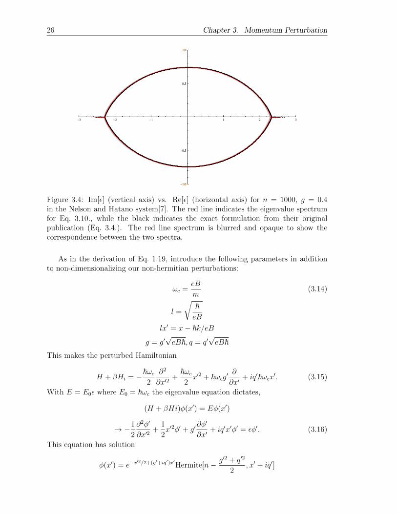
Figure 3.4: Im[] (vertical axis) vs. Re[] (horizontal axis) for n = 1000, g = 0.4in the Nelson and Hatano system[7]. The red line indicates the eigenvalue spectrumfor Eq. 3.10., while the black indicates the exact formulation from their originalpublication (Eq. 3.4.). The red line spectrum is blurred and opaque to show thecorrespondence between the two spectra.

As in the derivation of Eq. 1.19, introduce the following parameters in additionto non-dimensionalizing our non-hermitian perturbations:

ωc =eB

m(3.14)

l =

eB

lx = x− k/eB

g = g√eB, q = q

√eB

This makes the perturbed Hamiltonian

H + βHi = −ωc

2

∂2

∂x2 +ωc

2x2 + ωcg

∂

∂x + iqωcx

. (3.15)

With E = E0 where E0 = ωc the eigenvalue equation dictates,

(H + βHi)φ(x) = Eφ(x)

→ −1

2

∂2φ

∂x2 +1

2x2φ + g

∂φ

∂x + iqxφ = φ

. (3.16)

This equation has solution

φ(x) = e−x

2/2+(g+iq

)xHermite[n− g

2 + q2

2, x

+ iq]

27

⇒ φ(x) ≈ e−x

2/2+(g+iq

)xHn[x

+ iq].

Replacing x = x/l − kl with the non-dimensionalized X = x/l yields,

φ(X) = e− (X−kl2)2

2 +(g+iq)(X−kl

2)Hn[X − kl

2 + iq]. (3.17)

To examine the behavior of the g and q perturbations, the g parameter needs tobe held constant while q is varied and vice-versa. Setting the non-examined variableto 0 yields two equations:

φg(X) = e− (X−kl2)2

2 +g(X−kl2)Hn[X − kl

2], (3.18)

φq(X) = e− (X−kl2)2

2 +iq(X−kl2)Hn[X − kl

2 + iq]. (3.19)

The analytic eigenvectors for φ(x) are shown in Fig. 5.0.1.What happens to the eigenvalues under the momentum perturbation in Eq. 3.2?

Substituting Px → Px + ig, Py = ky → η + iq the y wave function cancels out asbefore,

E0(eag Ψ(x+ a, y) + e

−ag Ψ(x− a, y)

+ e− ieBxa

+aq +iηΨ(x, y + a) + e

ieBxa −aq

−iηΨ(x, y − a))

= EΨ(x, y) (3.20)

We want our equation in terms of non-dimensionalized, non-hermitian perturba-tions and α. To this end, note that,

ag

=ag

√eB = g

√2πα. (3.21)

Applying the same logic to the perturbation q and canceling the overall einη term, wefind the perturbed Hamiltonian,

eg√2πα

φ(m+1)+2 cos[2mπα−η− i

√2παq]φ(m)+e

−g√2πα

φ(m−1) = φ(m). (3.22)

H3 =

2 cos(2πα− η − i

√2παq) e

√2π

√αg

e

√2π

√α(−g)

e

√2π

√α(−g) 2 cos

4πα− η − i

√2παq

e

√2π

√αg

e

√2π

√α(g)

e

√2π

√α(−g) 2 cos(6πα− η − i

√2παq)

Figure 3.5: The 3x3 Hamiltonian describing the perturbed Harper’s equation for athree site lattice in Eq. 3.22.

Note that Eq. 3.22. can be converted into the form of Eq. 3.1. for q = 0 for H0

and Hi defined,

H0 = φ(m− 1) + φ(m+ 1) + 2 cos[2mπα− η]φ(m), (3.23)

andβHi =

eg√2πα − 1

φ(m− 1) +

e−g

√2πα − 1

φ(m+ 1). (3.24)

28 Chapter 3. Momentum Perturbation

Enforcing q = 0 to maintain the general form of a non-hermitian perturbation hintsat an inherent problem with the y perturbation. We will return to that instabilityfor q in the results section.

A cursory examination of Eqs. 3.23. and 3.24. in relation to Eqs. 3.11. and 3.12.shows how very similar the two systems are. Both the perturbations and the groundstates of each take the same basic form, with the only difference being the choiceof potential (random versus deliberate). Because the Nelson-Hatano system exhibitssuch a characteristic and clean phase transition, this indicates that our system hasa good chance of exhibiting non-hermitian behavior and possibly a phase transition.The hint of interesting non-hermitian is despite the general consensus that the quan-tum Hall Hamiltonian exhibits no unusual non-hermitian behavior, with at least onepublished source maintaining that the Harper system is robust against non-hermitianperturbation[22].

Chapter 4

Computation

4.1 Energy Eigenvalues

From the Harper’s equation (Eq. 3.22.), we have the following set of equations,

φ2 + 2 cos[2πα− η]φ1 + φn = φ1,

φ3 + 2 cos[4πα− η]φ2 + φ1 = φ2,

...

φ1 + 2 cos[2nπα− η]φn + φn−1 = φn.

For an n-dimensional lattice, the energy eigenvalues for non-dimensionalizedH satisfythe following equation,

Hφ = φ, (4.1)

where is simply some number. H can be written in matrix form,

H =

2 cos[2πα− η] 1 0 ... 1.1 2 cos[4πα− η] 1 ... ...

0. ... ... ... ...

... ... 1 2 cos[2(n− 1)πα− η] 11. ... ... 1 2 cos[2nπα− η]

. (4.2)

as well as the φ vector,

|φ =

φ1

φ2

...

...

φn

. (4.3)

To find the eigenvalues of H in Eq. 3.22 for various lattice sizes, we need to createthe Hamiltonian matrix to find the locations of phase transitions for both q and g.The general form of the perturbed energy system matrix is

H =

2 cos[2πα− η − q

√2πα] e

−g√2πα

...

eg√2πα 2 cos[4πα− η − q

√2πα] e

−g√2πα · ··

... ... ...

, (4.4)

30 Chapter 4. Computation

Figure 4.1: Two mathematica scripts used to find eigenvalues and manipulate data.The script “newnnh” creates the n× n perturbed Hamiltonian matrix correspondingto the perturbed harper’s equation on a continuous n-site lattice. “hofstadter” createsthe Hamiltonian matrix for the ground case (where there is no non-hermitian term).

Where the diagonals have exponential terms as well. We aren’t particularly interestedin how the spectrum changes for η, so we can set that parameter to 0. The solutionfor is a set of values that can take on to make the equation hold true. For an n×m

lattice there are n separate eigenvalues. Finding the set of solutions is a problemof finding a linear solution to n differential equations with three terms each (asidefrom the first and last equations that hold two terms each). Creating a program todo such a task is trivial, yet also uses methods that are computationally expensive.Instead, it is much faster to use Mathematica’s built-in function “Eigenvalues” to find that solve Eq. 4.1.

4.1. Energy Eigenvalues 31

Figure 4.2: Mathematica scripts used to plot eigenvalues. “inhh” computes the eigen-value spectra that make up the perturbed hofstader butterfly (in steps da = dα).“inhh” has an imaginary counterpart, “imhh”, that performs the same function butonly shows the imaginary parts of the resulting butterfly.

Figure 4.3: The code for the script “reimdat”, written in Mathematica. “reimdat”calculates the eigenvalues for the perturbed harper’s equation and returns the list ofIm[], Re[]. This data can then be plotted to indicate where an energy eigenvaluehas become complex.

Chapter 5

Results

The eigenvalues of Harper’s equation, when unperturbed, yield a fractal structure forthe eigenvalues as the flux quantum α is varied. For all nonzero values of q, the energyspectrum for Eq. 3.22. is immediately complex for all α values. However, g perturba-tions produce a transition between real and complex eigenvalues as g increases. Thisis a novel result for the harper’s equation.

5.0.1 Analytic Eigenfunctions

Figure 5.1: Plots of φ(x) for n = 2, and P → (Px+ ig)x+(Py+ iq)y, from Eqs. 3.18.and 3.19.

34 Chapter 5. Results

5.0.2 Hofstadter Butterflies

Figure 5.2: The unperturbed Hofstadter butterfly for n = 200.

35

Figure 5.3: The real spectra of the perturbed Hofstadter butterfly for n = 200,g = 0.25.

Figure 5.4: The imaginary spectra of the perturbed Hofstadter butterfly for n = 200,g = 0.25.

36 Chapter 5. Results

Figure 5.5: The real spectra of the perturbed Hofstadter butterfly for n = 200,q = 0.25.

Figure 5.6: The imaginary spectra of the perturbed Hofstadter butterfly for n = 200,q = 0.25.

37

5.0.3 Real vs. imaginary Eigenvalues

What follows here are plots of the real vs. imaginary eigenvalue spectrum for givenα, q and g parameters, over a 1000 site continuous lattice. Blue graphs represent gperturbations, while orange graphs represent q perturbations. In each plot of eachfigure, the set of numbers indicates its parameters like so: α, g, q.

Figure 5.7: Real vs. imaginary eigenvalue plots for α = 0.2 on a 1000-site lattice.Blue pertains to g (x) perturbation and orange to q (y) perturbation

38 Chapter 5. Results

Figure 5.8: Real vs. imaginary eigenvalue plots for α = 0.411 on a 1000-site lattice.Blue pertains to g (x) perturbation and orange to q (y) perturbation

39

Figure 5.9: Real vs. imaginary eigenvalue plots for α = 0.726 on a 1000-site lattice.Blue pertains to g (x) perturbation and orange to q (y) perturbation

40 Chapter 5. Results

Figure 5.10: Real vs. imaginary eigenvalue plots for α = 0.8 on a 1000-site lattice.Blue pertains to g (x) perturbation and orange to q (y) perturbation.

41

Figure 5.11: Real vs. imaginary eigenvalue plots for α = 0.2 on a 1000-site lattice.Blue pertains to g (x) perturbation. As the g parameter increases on the order of10−15 at α = 0.2, the eigenvalue spectrum evolves beyond simple transformations(scaling, shifting, etc.). The bracketed term above each plot indicates the order ofthe perturbation (e.g. -16E is g = 10−16)

42 Chapter 5. Results

Figure 5.12: Real vs. imaginary eigenvalue plots for α = 0.4 on a 1000-site lattice.Blue pertains to g (x) perturbation. A move from all-real to complex eigenvaluesappears while varying g on the order of 10−15 at α = 0.4. The bracketed term aboveeach plot indicates the order of the perturbation (e.g. -16E is g = 10−16)

43

Figure 5.13: Real vs. imaginary eigenvalue plots for α = 0.2 on a 1000-site lattice.Orange pertains to q (y) perturbation. The eigenvalue spectrum scales with q. Despiteusing the same system parameters as the g perturbation, there appears to be no analogto the g eigenvalue evolution for q on the order of 10−15 at α = 0.2. The bracketedterm above each plot indicates the order of the perturbation (e.g. -16E is g = 10−16).

44 Chapter 5. Results

Figure 5.14: Real vs. imaginary eigenvalue plots for α = 0.4 on a 1000-site lattice.Orange pertains to q (y) perturbation. There appears to be no analog to the g

eigenvalue evolution for q on the order of 10−15 at α = 0.4. The eigenvalue spectrumsimply scales with q. The bracketed term above each plot indicates the order of theperturbation (e.g. -16E is g = 10−16).

Conclusion

As with other systems, the non-hermitian parameters g and q can be interpretedas coupling terms. Further, the qualitative behavior of the analytic eigenvectorsmay indicate how energy moves within the lattice. With increasing g the analyticeigenvectors skew the wave functions back along the lattice. As shown in Fig 3.5.,x-perturbations manifest themselves in the coefficients for the cross terms. Withincreasing α, the coupling of the g(m − 1) term decreases, and the coupling of theg(m+ 1) increases, porting a larger amount of energy forward on the lattice.

It is not surprising, therefore, that there may be no phase transition for the q pa-rameter. For all non-zero q, cos[β− iq

√2πα] is complex, indicating a complex energy

state. The equation considers only the direction perpendicular to this perturbation’sdirectional origins. It is possible that when replaced into an equation without thesquare lattice ansatz in Eq.1.17, it might exhibit a phase transition. Perhaps, however,the gauge choice pointing the magnetic vector potential in the y direction forces anycomplex perturbation in that direction to create energy eigenvalues. Interestingly, qperturbations seem to exactly copy the behavior of g perturbations for certain α val-ues, exhibiting what may be phase transitions. It also appears, however, that certainvalues of α completely barr the possibility of a phase transition (Compare Figs. 5.7and 5.10 with Figs. 5.8 and 5.9.).

The character of the possible phase transition in g is defined by two regions: stableand unstable. Within the stable regime, there exist some values for g such that theresulting energy spectrum is complex, but these values are localized and do not affectthe spectrum significantly. For example, the imaginary portions of the eigenvaluespectrum for α = 0.4 (Fig. 5.12) continue to be insignificant with respect to the realpart of the eigenvalues well after they appear. For the first complex eigenspectrumfound for a given set of parameters, the imaginary values tend to be so incrediblysmall and so fleeting that they can be discounted without too much justification.

According to the Nelson-Hatano literature, where the perturbing parameter be-comes sufficiently large, all states, including the ground state, translate into the com-plex domain. While confirming this fact extends beyond the reach of this document,Fig 5.9. bears the mark that such a phase transition has or may yet occur. Abovesome critical value for the system, there are only two real eigenvalues for the system.Qualitatively, the middle states have seemed to merge together and ballooned out, nolonger crossing the real plane. The imaginary eigenspectrum suddenly surges to theorder of the real eigenspectrum, indicating a non-trivial phase transition for the entiresystem, similar to the features and behavior of the Nelson-Hatano system (Fig. 3.4).

46 Conclusion

The possibility of a PT-phase transition for the g parameter is novel and well-supported by the Nelson-Hatano model. The only difference between the non-hermitianHamiltonian for random potentials and the perturbed Harper’s equation is the pre-determined potential functions contained in Harper’s equation. Furthermore, thesystem described by the perturbed Harper’s equation has its root in the analyticsolution of a shifted quantum harmonic oscillator. Since the two coupled oscillatorsystems outlined in the PT-quantum mechanics section outline an excellent and cleanexample of a PT-phase transition it would not be a surprise that a system of n-suchcoupled oscillators would also exhibit a phase transition.

Unlike with the non-hermitian coupled systems examined in the PT quantummechanics section, the momentum-perturbed quantum Hall system pertains to verycomplex coupling dynamics whose exact behavior is unclear. A physical examplemight couple a number of quantum harmonic oscillator systems and observe thedynamics of each pendulum individually to see if some of the oscillators maintainPT-symmetric behavior while others do not. Further, it would look for a criticalarea or value beyond which the entire system observes a phase transition, a possiblephysical manifestation of broken PT-symmetry.

Appendix A

Derivations

A.0.4 Hermite Polynomials

Solving the differential equation describing the behavior of a particle in a magneticfield requires a few tricks. Solving Eq. 1.22. means solving a an equation of the form,

φ − x

2φ− 2φ = 0 (A.1)

This class of equations can via at least two methods: by assuming that φ is somefunction multiplied by a power series in x, and through a method of ladder operators[23]. I use a combination of the two to find the restriction on , then to find the finalform of φ. To begin, notice that for x → ∞,

φ − x

2φ ≈ 0 (A.2)

Suggesting a solution of the form,

φ = u[x]e−x2/2 (A.3)

Applying this ansatz in A.2. eventually becomes,

e−x2

2 ((2− 1)u[x] + u[x]− 2xu[x]) = 0 (A.4)

Now, assume that u is a power series in x,

u =∞

i=0

αixi. (A.5)

The expression from A.4 becomes

(2− 1)∞

i=0

aixi +

∞

i=0

(i− 1)iaixi−2 − 2x

∞

i=0

iaixi−1 = 0,

⇒ (2− 1)∞

i=0

aixi +

∞

i=0

(i− 1)iaixi−2 − 2

∞

i=0

iaixi = 0,

48 Appendix A. Derivations

⇒∞

i=0

(2− 1− 2i)aixi +

∞

i=0

(i− 1)iaixi−2 = 0.

Now, there is some lowest coefficient such that al = 0. The first two terms of thexi−2 sum should therefore be 0, so the iterator can therefore be changed i → i+ 2 in

the right sum, while still starting from i = 0. Updating the iterator yields,

∞

i=0

(2− 1− 2i)aixi −

∞

i=0

(i+ 1)(i+ 2)ai+2xi = 0

We can now bring both terms inside the summation, finally yielding the equality,

(i+ 1)(i+ 2)ai+2 = (2− 1− 2i)ai

This equation diverges, which represents a non-physical solution (infinite wavefunction). Therefore, we ask that the wave function have some finite level n suchthat

an+2 =2− 1− 2n

(n+ 1)(n+ 2)an = 0 (A.6)

This can be done by making the numerator zero,

2− 1− 2n = 0. (A.7)

The condition implies that take the following value,

= n+ 1/2. (A.8)

Thus, the energy levels are quantized for a particle in a magnetic field. Havingfound the condition of energy quantization, we use the ladder operator method togenerate wave functions easily (see [23] for a thorough treatment of the ladder operatormethod). Rewriting Eq. 1.22. with the constraint in A.8,

φ − x

2φ = (2n+ 1)φ. (A.9)

We can rewrite this equation in terms of the derivative operators:

D =∂

∂x.

Now,. A.9 can be factored into two equations involving D,

(D − x)(D + x)φn = −2nφn, (A.10)

And,(D + x)(D − x)φn = −2(n+ 1)φn. (A.11)

To see how the operators (D+x) and (D−x) affect the wave function, consider whathappens to the differential equation for some other wave function φm when actedupon by (D + x) and (D − x). From A.10,

(D + x)(D − x)(D + x)φm = −2m(D + x)φm. (A.12)

49

From A.11,(D − x)(D + x)(D − x)φm = −2(m+ 1)(D − x)φm. (A.13)

Compare A.10 and A.12. The equations are identical for, yn = [(D − x)ym] andn = m+ 1, implying,

ym+1 = (D − x)ym. (A.14)

.Similarly, for A.10 and A.12, yn = [(D + x)ym], and n = m− 1,

ym−1 = (D + x)ym. (A.15)

These equations are called ladder operators. They take any yi to yi+1 or yi−1

except where there is no higher or lower rung. For instance, there should be somelowest function φ0 such that,

(D + x)φ0 = 0. (A.16)

Solving this equation yields,

φ0 = e−x2

2 . (A.17)

With this equation, in conjunction with A.14., any wave function can be created. φ1

for example:

φ1 = (D − x)φ0 = A(D − x)e−x2

2 .

The equation for some φi, for general i, is therefore,

φi = A(D − x)ie−x2

2 . (A.18)

Or, in its equivalent form,

φn = Ae−x2

2 Hn(X) = A(−1)ne−x2

2 ex2 ∂

n

∂xne−x

2. (A.19)

Hn(x) are the Hermite polynomials. Now that we have the full form of the solution, weneed to orthonormalize it. The Hermite polynomials are already orthogonal, meaning,

∞

−∞Hn[x]Hm[x]dx = 0 m = n

1 n = m. (A.20)

With the Hermite polynomials are already orthogonal, the full solution is orthogonalas well. However, the full solution still needs to be normalized over x[∞,∞]. Fornormalization of each wave function, we want,

1 =

∞

−∞|φ∗

φ|dx

The conjugate of some φn is simply φn,

1 = A

∞

−∞e−x

2Hn[x]Hn[x]dx. (A.21)

50 Appendix A. Derivations

Expanding the first Hermite polynomial yields,

1 = A2(−1n)

∞

−∞

∂n

∂xn

e−x

2Hn[x]dx. (A.22)

Integrating by parts, we have,

1 = −A2(−1)n−1

∂n

∂xn[e−x

2]Hn[x]

∞

−∞− 2

∞

−∞

∂n−1

∂xn−1

e−x

2Hn[x]dx

. (A.23)

The left part of the equation is 0 at its endpoints, leaving the integral on theright which can be further integrated by parts until in the same manner until theH0(x) polynomial, which is 1. Furthermore, there is a factor of (−1)n from theseintegrations by parts, since each integral has a negative sign. This factor combineswith the leading (−1)n to make (−1)2n = 1. After these steps, we are left with,

1 = A2

∞

−∞e−x

2Hn[x]dx. (A.24)

Integrating by parts yet again,

1 = A2

e−x

2Hn(x)

∞−∞

− ∞

−∞e−x

2H

n[x]dx

. (A.25)

Yet again, the left side is 0. Now, using the relation Hn(x) = 2nHn−1(x)[23],

1 = A22n

∞

−∞e−x

2Hn−1(x)dx, (A.26)

1 = A222n(n− 1)

∞

−∞e−x

2Hn−2(x)dx,

.

.

.

1 = A22nn!

∞

−∞e−x

2dx = A

22nn!.√π (A.27)

Finally, we have the constant A to normalize the wavefunction φn:

A =1√

2nn!π1/2. (A.28)

Finally, from A.19 and A.28, comes the form of φn,

φn(x) =1√

2nn!π1/2e−x

2/2Hn(x). (A.29)

51

A.0.5 Longitudinal Current[4]

Beginning from

Iy =

J(r) · xdy, (A.30)

Iy =1

L

Jy(x, y)dxdy, (A.31)

Iy = − e

L

d2pvy, (A.32)

Iy = − e

L

j

vy. (A.33)

From Eq. 1.11. get the form of vy, making the current expression,

Iy = − e

2π

dpyvpy np (A.34)

Which is equivalent to Eq. 1.35.

References

[1] D.J. Griffiths. Introduction to Quantum Mechanics. Pearson Prentice Hall, 2005.

[2] J. Von Neumann. Mathematical Foundations of Quantum Mechanics, Translated

by Beyer, R. T. Princeton University Press, 1971.

[3] C. M Bender. Introduction to pt-symmetric quantum theory. Contemporary

Physics, 46(4):277–292, 2005.

[4] J.K Jain. Composite Fermions. Cambridge:Cambridge University Press, 2007.

[5] Antikon. Quantum hall effect–russian.png. Wikipedia:GNU Free Documentation

License, Dec 2005.

[6] D. R. Hofstadter. Energy levels and wave functions of bloch electrons in rationaland irrational magnetic fields. Phys. Rev. B, 14:2239–2249, Sep 1976.

[7] N. Hatano and D. R. Nelson. Non-Hermitian delocalization and eigenfunctions.prb, 58:8384–8390, October 1998.

[8] E. H. Hall. On a new action of the magnet on electric currents. American Journal

of Mathematics, 2:287–292, Sep 1879.

[9] K. v. Klitzing, G. Dorda, and M. Pepper. New method for high-accuracy deter-mination of the fine-structure constant based on quantized hall resistance. Phys.Rev. Lett., 45:494–497, Aug 1980.

[10] Klaus Klitzing. 25 years of quantum hall effect (qhe) a personal view on thediscovery, physics and applications of this quantum effect. 45:1–21, 2005.

[11] D. C. Tsui, H. L. Stormer, and A. C. Gossard. Two-dimensional magnetotrans-port in the extreme quantum limit. Phys. Rev. Lett., 48:1559–1562, May 1982.

[12] D. Seiler R. Avron, J. E Osadchy. A topological look at the quantum hall effect.

[13] B. I. Halperin. The quantized Hall effect. Scientific American, 254:52–60, April1986.

[14] K. Jones-Smith. Non-Hermitian Quantum Mechanics. Phd. thesis, Case WesternReserve University, May 2010.

54 References

[15] C. M. Bender and S. Boettcher. Real Spectra in Non-Hermitian HamiltoniansHaving PT Symmetry. Phys. Rev. Lett., 80:5243–5246, June 1998.

[16] C. M. Bender. Making sense of non-Hermitian Hamiltonians. Reports on Progress

in Physics, 70:947–1018, June 2007.

[17] S. Bittner, B. Dietz, U. Gunther, H. L. Harney, M. Miski-Oglu, A. Richter, andF. Schafer. pt symmetry and spontaneous symmetry breaking in a microwavebilliard. Phys. Rev. Lett., 108:024101, Jan 2012.

[18] C. M. Bender, B. K. Berntson, D. Parker, and E. Samuel. Observation of phasetransition in a simple mechanical system. American Journal of Physics, 81:173–179, March 2013.

[19] Joseph Schindler, Ang Li, Mei C. Zheng, F. M. Ellis, and Tsampikos Kottos.Experimental study of active lrc circuits with pt symmetries. Phys. Rev. A,84:040101, Oct 2011.

[20] N. Hatano and D. R. Nelson. Vortex pinning and non-hermitian quantum me-chanics. Phys. Rev. B, 56:8651–8673, Oct 1997.

[21] F. Hbert, M. Schram, R. T. Scalettar, W. B. Chen, and Z. Bai. Hatano-nelsonmodel with a periodic potential. The European Physical Journal B, 79(4):465–471, 2011.

[22] A. Jazaeri and I. I. Satija. Localization transition in incommensurate non-Hermitian systems. pre, 63(3):036222, March 2001.

[23] M.L. Boas. Mathematical Methods in the Physical Sciences. Kaye Pace, 2005.

[24] O A Pankratov. Electronic properties of band-inverted heterojunctions: super-symmetry in narrow-gap semiconductors. Semiconductor Science and Technol-

ogy, 5(3S):S204, 1990.

[25] Igor N Karnaukhov. Phase transition in the PT -symmetric spin-1/2 quantumchain. Phys. Rev. A, 45(44):444018, 2012.

[26] N. Moiseyev. Non-hermitian quantum mechanics: Formalism and applications.Fundamental World of Quantum Chemistry, 2:1–32, 2003.

[27] Insel A. J. Spence L. E. Friedberg, S. H. Linear Algebra. PHI Learning PrivateLimited, 2003.

[28] T. Hollowood. Solitons in affine toda field theories. Nuclear Physics B, 384(3):523– 540, 1992.

[29] E. Schrodinger. Collected Papers on Wave Mechanics,. Chelsea Publishing Com-pany, 1982.