two-dimensional development of the dynamic coupled ... · coupled consolidation scaled boundary...
TRANSCRIPT

Loughborough UniversityInstitutional Repository
Two-dimensionaldevelopment of the dynamiccoupled consolidation scaled
boundary finite-elementmethod for fully saturated
soils
This item was submitted to Loughborough University's Institutional Repositoryby the/an author.
Citation: EL-HAMALAWI, A. and HASSANEN, M.A., 2007. Two-dimensionaldevelopment of the dynamic coupled consolidation scaled boundary finite-elementmethod for fully saturated soils. Soil Dynamics and Earthquake Engineering,27 (2), pp. 153-165.
Additional Information:
• This article was published in the journal, Soil Dynamics and Earth-quake Engineering [ c© Elsevier] and the definitive version is available at:www.elsevier.com/locate/soildyn
Metadata Record: https://dspace.lboro.ac.uk/2134/5159
Version: Accepted for publication
Publisher: c© Elsevier
Please cite the published version.

This item was submitted to Loughborough’s Institutional Repository (https://dspace.lboro.ac.uk/) by the author and is made available under the
following Creative Commons Licence conditions.
For the full text of this licence, please go to: http://creativecommons.org/licenses/by-nc-nd/2.5/

1
2D DEVELOPMENT OF THE DYNAMIC COUPLED CONSOLIDATION SCALED
BOUNDARY FINITE ELEMENT METHOD FOR FULLY SATURATED SOILS
A. El-Hamalawia, * and M. Hassanenb
a Civil & Building Engineering Department, Loughborough University, Loughborough
LE11 3TU, United Kingdom
b Department of Civil Engineering, Strathclyde University, 107 Rottenrow, Glasgow G4
0NG, UK
Abstract
The scaled boundary finite element method is a powerful tool used to analyse far-field
boundary soil-structure interaction problems. In this paper, the method is extended to
include Biot’s coupled consolidation in order to deal with fully saturated soil as a two-
phase medium. The advantages of this method are explained in this paper. The
detailed formulation considers the general 2D analysis case, accounting for body
forces and surface tractions in both bounded and unbounded media.
Keywords : scaled boundary finite element method, coupled consolidation, soil
mechanics, fully saturated.
1. Introduction
For a number of practical engineering applications such as very stiff and massive
structures, the numerical study of transient soil-structure interaction under dynamic
conditions is important. Most engineers in industry currently attempt to idealise these
* Corresponding author. Address : Civil & Building Engineering Department, Loughborough University,
Loughborough LE11 3TU, United Kingdom. Tel: +44-1509 223206; fax: +44-1509 223981
E-mail address: [email protected]

2
problems by performing a quasi-static analysis, and assuming that the soil in question
is a single-phase material. Saturated soil is however a multi-phase material and its
behaviour is governed by its main constituents: solid particles and pore fluids. As the
pore pressures build up with time, such as in an earthquake during liquefaction, the
structural response is affected significantly. To therefore produce a more realistic
representation of saturated soil under dynamic loads, a two-phase coupled solid-fluid
formulation is required. Several numerical methods exist to model dynamic soil-
structure interaction, but modelling the soil as a half-space has many shortcomings,
as described below.
Fig. 1. Layout of a typical dynamic soil-structure interaction problem
Fig. 1 shows an embedded structure overlying soil, which extends to infinity. The
problem constitutes the determination of the dynamic response of the structure
interacting with the soil, upon applying a time-varying load such as seismic waves in
an earthquake or vibrations due to machinery. The soil can be split into two parts: a
bounded near-field medium, which could comprise several layers, and an unbounded
far-field medium that extends to infinity. As the dynamic load takes effect, waves are
emitted and propagate throughout the soil in all directions either towards infinity or
towards the structure depending on the initial input waves’ source. The most important
question when idealising the soil domain is how to best model the infinite boundary.
Numerically, this has usually been achieved by truncating the remote boundaries and
then imposing free or fixed boundary conditions. If input waves originate at the
structure, and propagate through the soil towards infinity, the artificial far-field domain
boundary would reflect waves back into the near-field and structure, thus producing
erroneous results. Proper modelling of the far-field boundary is also very important at
3
high frequencies above the cut-off frequency, in order to provide a better
representation of the radiation damping that occurs. A proper quantification of the
level of radiation damping that exists would help engineers make use of this condition
when designing. Despite much progress in finite element technology, the requirement
for a computationally efficient technique that is able to capture accurately the 3-
dimensional stress wave transmission in anisotropic soils still posses an important
challenge within engineering mechanics.
One solution to this problem when using the "industry-standard" finite element method
(FEM) in analysing the problem would be to use an extended FE mesh with a large
number of elements to model the region where the stress waves may propagate
during the time scale of the analysis. This might provide a solution for short duration
transient problems, but with practical earthquake analyses, where the waves will
travel a great distance during earthquake excitation (say up to 30 seconds), an
excessive and impractical computational cost would be incurred. In 3D, an extended
mesh would require prohibitively high computer resources by today’s standards, and
would thus not be viable. In order to avoid this, different boundaries have been
developed to minimise wave reflections and absorb the wave energy, such as viscous
energy-absorbing boundaries [1], [2], or Smith boundaries [3]. These however have
not been entirely effective at simulating the far-field. Boundaries by Smith [3] were
restricted to applications having simple geometries, while the viscous energy-
absorbing boundary was ineffective for body waves with angles of incidence of less
than 30° and for surface waves. Bettess and Zienkiewicz [4] introduced infinite
elements to simulate the far-field boundary for wave propagation problems in single-
phase porous elastic media, followed by other researchers such as Chow and Smith
[5], and Zhao and Valliappan [6]. The element shape functions used are decay

4
functions representing the wave propagation towards infinity. Simoni and Schrefler [7],
and Khalili et al. [8] used infinite elements for wave propagation in 2-phase saturated
porous media. These approaches improved the modelling, but still do not provide an
accurate representation, as infinite elements are not exact in the finite-element sense,
so are less accurate than the remaining finite element near-field domain.
One method that overcomes the problems associated with modelling the far-field
boundary is the boundary element method (BEM). The fundamental solution required
for the BEM formulation would satisfy the radiation damping condition at the far-field
boundary exactly. Cheng and Liggett [9], and Cheng and Detournay [10], developed a
BEM formulation to model 2D static linear elastic consolidation formulated in the
Laplace transform space, using Cleary's fundamental solution [11]. Dargush and
Banerjee [12] extended this formulation to 3D. By using an analogy between
poroelasticity and thermoelasticity, different fundamental solutions were presented by
different researchers [13], [14], and used by Cheng et al. [10] and Dominguez [14] to
produce dynamic BEM formulations for poroelasticity. However, an understanding of
the boundary element method requires a rigorous theoretical mathematics
background not generally available to civil engineers. In addition, one of the major
drawbacks of the method is the necessity of a fundamental solution to exist. Such an
analytical solution is difficult to derive, and in some cases exhibits singularities, while
in other cases a fundamental solution does not exist. The latter makes it very
complicated and sometimes impossible to apply the BEM to problems involving
plasticity, except in the simplest of cases.
The finite-boundary element method (FBEM, e.g. [15]), is one method that combines
the advantages of both the FEM and BEM. The near-field is discretised into finite
elements, which allows any elastic or plastic constitutive model to represent the soil
without the need of a fundamental solution, while the far-field is modeled using the

5
BEM, which improves the modelling of the far-field boundary and radiation condition.
The application of the method however is not easy, and problems occur along the
interface separating the finite and boundary elements, and with layered soils.
The scaled boundary finite element method (SBFEM), developed by Wolf and Song
[16], overcomes many of these shortcomings when modelling the far-field boundary in
a dynamic soil-structure interaction situation. A scaling centre is chosen outside the
soil area as shown in Fig. 2, with the soil-structure interface split into 1D finite
elements. A typical finite element 1-2 is shown in Fig. 2 in relation to the scaling
centre O. A scaled transformation in coordinates is performed from the Cartesian to
the radial dimensionless coordinate ξ such that the unbounded far-field soil
corresponds to the domain 1 ξ≤ < ∞ and the bounded near-field area corresponds to
the domain 0 1ξ≤ ≤ . In the frequency domain, the governing differential equations of
elastodynamics are transformed into a system of linear second-order ordinary
differential equations, either by using the weighted-residual method [17], or by using
the concept of similarity [16]. After defining the dynamic stiffness, a system of non-
linear first-order ordinary differential equations results, which is solved for the dynamic
stiffness matrix as a function of frequency. A similar derivation process yields the
unit-impulse response matrix in the time domain. At high frequencies above the cut-off
frequency, the use of an asymptotic expansion to represent the dynamic-stiffness
matrix yields a boundary condition satisfying the far-field radiation condition exactly.
The computed solutions are exact in a radial direction (from the soil-structure
boundary pointing towards infinity), while converge to the exact solution in the finite
element sense in the circumferential direction parallel to the soil-structure boundary
interface. From a computational point of view, the SBFEM results in symmetric
dynamic-stiffness and unit-impulse response matrices, which would not be the case if
the BEM or FBEM were used, making it much more efficient time and storage-wise.

6
A major advantage for both the academic and engineer in industry is during the initial
discretisation of the problem to be analysed, where similar to the BEM, only the
boundary rather than the domain needs discretisation. This means that for 3D
problems, 2D surface finite elements are used to discretise the boundary, which result
in reducing the spatial dimension by one, and in turn the number of degrees of
freedom during the analysis. It also allows very complicated 3D meshes to be
discretised easily (overcoming the problems inherent in approximating 3D problems
into 2D) and removes the significant time burden associated with generating a 3D
mesh. Although 2D modelling of a 3D model is convenient, it has many problems such
as the contact area for 2D problems being larger (e.g. if plane strain is assumed) than
in 3D, which will overestimate radiation damping for frequencies above the cut-off
frequency. As with the BEM, by not discretising the domain, internal displacements
and stresses are computed more accurately than with the FEM. However, in contrast
to the BEM, the behaviour of the bounded near-field soil can be represented in the
SBFEM using any advanced constitutive model (for example, based on plasticity).
This is due to the SBFEM not requiring a fundamental solution, unlike the
BEM/FEBEM, which also eliminates the need to evaluate singular integrals occurring
in most fundamental solutions. Anisotropy can also be modelled using the SBFEM
without an increase in computational effort. The advantages of the FEM and BEM are
thus combined. The method currently exists for single-phase media. A more accurate
representation of the far-field boundary during a dynamic soil-structure interaction
analysis would be acieved by extending it to account for two-phase media. The aim of
this paper is to develop a numerical formulation capable of correctly modelling the
dynamic far-field boundary condition for two-phase media, and study its effect on the
time-dependent interaction between a structure, and the underlying local soil.

7
2. Governing Equations
The scaled boundary finite element method (SBFEM) equations derived in the past
have been based on the equilibrium equations (e.g. [18]). In this section, the
formulation will be re-derived to incorporate the process of consolidation in the soil.
This is especially important in geotechnical engineering as it accounts for the
changing pore water pressures that occur in between the drained and undrained
states. The standard SBFEM formulation would only allow the modelling of soils in the
long-term (drained) case, or short-term (undrained) with some modification to the
formulation to take into consideration the pore water pressures, which are a function
of volumetric strain during the undrained case. This however would not be satisfactory
for most soils undergoing the crucial intermediate consolidating stage.
The coupled consolidation equations [19] comprise a system of simultaneous
differential equations which satisfy; (a) the dynamic equilibrium equations of motion
and (b) the fluid continuity equations. The following 2-dimensional differential
equations of motion (expressed in terms of displacement amplitudes) are exact in the
frequency domain.
0)(
ˆ)(
=+−′∂
+∂+
∂+′∂
xxxyx buy
px
pρρ
τσ&&
(1)
0ˆ
)()(=+−
∂
+∂+
′∂
+′∂yy
xyy bux
py
pρρ
τσ&&
where σ ′ is the effective stress, p is the fluid pressure (in which the total stress, σ ,
relates to the fluid pressure as { } { } { }pm+′= σσ ), u is the displacement, ω and ρ are
the frequency and density respectively, and { }b is a vector representing the body
forces per unit volume.

8
The fluid continuity equation is shown below :
0)
ˆˆ()
ˆˆ()
ˆˆ()
ˆˆ( 2
2
2
2
2
=+∂
∂+
∂∂
+∂
∂+
∂∂
+∂
∂+
∂∂
+∂∂
+∂∂
− pKni
yu
xu
iyb
xb
kyu
xu
kyp
xpk
f
yxyxf
yxf ωωρρω (2)
where p is the fluid pressure , u , ω , k, n, Kf and ρ are the displacement, frequency,
soil permeability and porosity, fluid bulk modulus and density respectively, and { }b is
the body forces per unit volume vector.
3. Scaled Boundary Finite Element Transformation of Geometry
Fig. 2. Scaled boundary transformation of geometry of line finite element
Consider a finite line element 1-2 forming the base of the triangle in Fig. 2 with the
opposite apex of the triangle coinciding with the scaling centre O and the origin of the
Cartesian coordinates system. Any point A on the boundary line element 1-2, with
local coordinates (x, y) , can be represented by its position vector r ,
jir yx += (3)
If the origin, O , of the Cartesian coordinates ˆ ˆ(x, y) coincides with the apex of the
triangle, then a point within the domain may be described in Cartesian coordinates by
its global position vector r as
jir yx ˆˆˆ += (4)
9
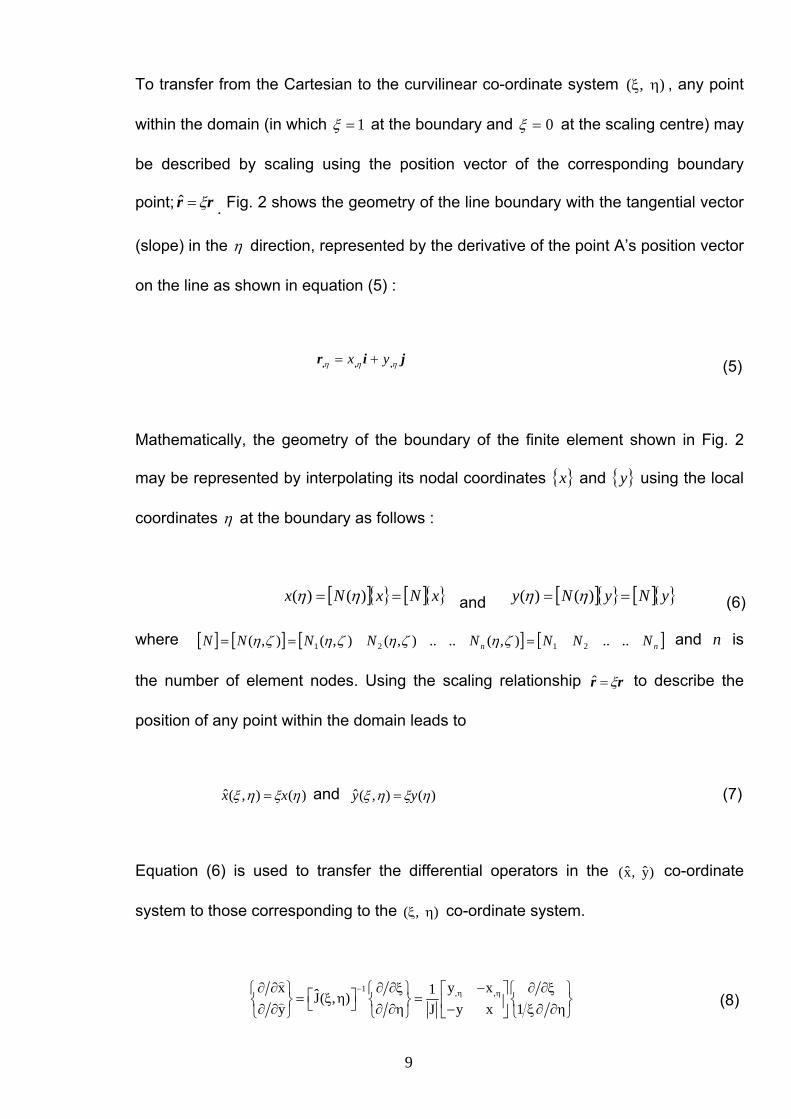
To transfer from the Cartesian to the curvilinear co-ordinate system ( , )ξ η , any point
within the domain (in which 1=ξ at the boundary and 0=ξ at the scaling centre) may
be described by scaling using the position vector of the corresponding boundary
point; rr ξ=ˆ . Fig. 2 shows the geometry of the line boundary with the tangential vector
(slope) in the η direction, represented by the derivative of the point A’s position vector
on the line as shown in equation (5) :
jir ,,, ηηη yx += (5)
Mathematically, the geometry of the boundary of the finite element shown in Fig. 2
may be represented by interpolating its nodal coordinates { }x and { }y using the local
coordinates η at the boundary as follows :
[ ]{ } [ ]{ }xNxNx == )()( ηη and [ ]{ } [ ]{ }yNyNy == )()( ηη (6)
where [ ] [ ] [ ] [ ]nn NNNNNNNN ....),(....),(),(),( 2121 === ζηζηζηζη and n is
the number of element nodes. Using the scaling relationship rr ξ=ˆ to describe the
position of any point within the domain leads to
)(),(ˆ ηξηξ xx = and )(),(ˆ ηξηξ yy = (7)
Equation (6) is used to transfer the differential operators in the ˆ ˆ(x, y) co-ordinate
system to those corresponding to the ( , )ξ η co-ordinate system.
1 , ,x y x1J( , )y y x 1J
− η η∂ ∂ ∂ ∂ξ − ∂ ∂ξ⎧ ⎫ ⎧ ⎫ ⎡ ⎤ ⎧ ⎫⎡ ⎤= ξ η =⎨ ⎬ ⎨ ⎬ ⎨ ⎬⎢ ⎥⎣ ⎦∂ ∂ ∂ ∂η − ξ∂ ∂η⎩ ⎭ ⎩ ⎭ ⎣ ⎦ ⎩ ⎭
)
) (8)

10
where the Jacobian matrix is [ ] ⎥⎦
⎤⎢⎣
⎡=
ηη
ξξηξ,,
,,
ˆˆˆˆ
),(ˆyxyx
J and the determinant is ηη ,, yxxyJ −= .
At 1=ξ , on the curved boundary, the unit outward normal vector is defined by
equation (9).
][1,, jijign ηηξ
ξξξ
ξξ xy
gnn
g yx −=+== where jirg , ηηη
ξ,, xy −==
(9)
Similarly, the unit outward normal vector to the line )(ξ is :
][1 jijign xyg
nng yx +−=+== η
ηηη
ηη
where jirg xy +−==η
(10)
where 2,
2, )()( ηη
ξξ xyg −+== g and 22 )()( xyg +−== ηη g . Substituting the derivative
relationships results in :
⎥⎥⎥⎥
⎦
⎤
⎢⎢⎢⎢
⎣
⎡
∂∂
∂∂
∂∂
∂∂
=
⎪⎪⎭
⎪⎪⎬
⎫
⎪⎪⎩
⎪⎪⎨
⎧
∂∂
∂∂
⎥⎥⎦
⎤
⎢⎢⎣
⎡=
⎪⎪⎭
⎪⎪⎬
⎫
⎪⎪⎩
⎪⎪⎨
⎧
∂∂∂∂
ηξξ
ηξξ
ηξ
ξηηξξ
ηηξξ
ηηξξ
ηηξξ
yy
xx
yy
xx
ngng
ngng
Jngngngng
Jy
x1
11
11
ˆ
)
(11)
3.1 The Equilibrium Equations of Motion
For harmonic motion, the velocity and acceleration may be represented by
uituu ω=∂∂
=& and utuu 22
2
ω−=∂∂
=&& respectively.
The equilibrium equations (1) may thus be rewritten as
11
0)(
ˆ)( 2 =++
′∂
+∂+
∂+′∂
xxxyx buy
px
pρρω
τσ
0ˆ
)()( 2 =++∂
+∂+
′∂
+′∂yy
xyy bux
py
pρρω
τσ (12)
In vector notation;
[ ] { } { }( ) { } { } 02 =+++′ bupmL T ρρωσ (13)
where for the 2-dimensional case;
{ }⎥⎥⎥
⎦
⎤
⎢⎢⎢
⎣
⎡=
011
m , total normal stress = { }⎪⎭
⎪⎬
⎫
⎪⎩
⎪⎨
⎧=
τσσ
σ
xy
y
x
, strain = { }⎪⎭
⎪⎬
⎫
⎪⎩
⎪⎨
⎧
=γεε
ε
xy
y
x
, { } ⎥⎦
⎤⎢⎣
⎡=
uuu
y
x ,{ } ⎥⎦
⎤⎢⎣
⎡=
bbb
y
x
and [ ]⎥⎥⎥
⎦
⎤
⎢⎢⎢
⎣
⎡
∂∂∂∂∂∂
∂∂=
xyy
xL
))
)
)
00
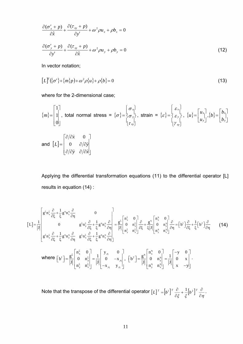
Applying the differential transformation equations (11) to the differential operator [L]
results in equation (14) :
[ ]
x x
x x1 2
y y y y
y x y x
y y x x
1g n g n 0n 0 n 0
1 1 g g 1L 0 g n g n 0 n 0 n b bJ J J
n n n n1 1g n g n g n g n
ξ ξ η η
ξ ηξ η
ξ ξ η η ξ η
ξ ξ η η
ξ ξ η η ξ ξ η η
⎡ ⎤∂ ∂+⎢ ⎥∂ξ ξ ∂η⎢ ⎥ ⎡ ⎤ ⎡ ⎤
⎢ ⎥∂ ∂ ∂ ∂ ∂ ∂⎢ ⎥ ⎢ ⎥ ⎡ ⎤ ⎡ ⎤= + = + = +⎢ ⎥ ⎢ ⎥ ⎢ ⎥ ⎣ ⎦ ⎣ ⎦∂ξ ξ ∂η ∂ξ ξ ∂η ∂ξ ξ ∂η⎢ ⎥ ⎢ ⎥ ⎢ ⎥⎣ ⎦ ⎣ ⎦⎢ ⎥∂ ∂ ∂ ∂+ +⎢ ⎥∂ξ ξ ∂η ∂ξ ξ ∂η⎣ ⎦
(14)
where
x , x
1 2y , y
y x , , y x
n 0 y 0 n 0 y 0g 1 g 1b 0 n 0 x , b 0 n 0 xJ J J J
n n x y n n x y
ξ ηηξ η
ξ ηη
ξ ξ η ηη η
⎡ ⎤ ⎡ ⎤⎡ ⎤ −⎡ ⎤⎢ ⎥ ⎢ ⎥⎢ ⎥ ⎢ ⎥⎡ ⎤ ⎡ ⎤= = − = =⎢ ⎥ ⎢ ⎥⎣ ⎦ ⎣ ⎦⎢ ⎥ ⎢ ⎥⎢ ⎥ ⎢ ⎥⎢ ⎥ ⎢ ⎥− −⎣ ⎦⎣ ⎦⎣ ⎦ ⎣ ⎦
.
Note that the transpose of the differential operator [ ] [ ] [ ]ηξξ ∂∂
+∂∂
=TTT bbL 21 1 .

12
Applying the transformation in equation (14) to the differential equation of motion
yields
[ ] { } [ ] { } [ ] { } [ ] { } { } { } 011 2,
2,
1,
2,
1 =++++′+′ bupmbpmbbb TTTTρρω
ξσ
ξσ ηξηξ (15)
3.2 The Fluid Continuity Equation
The fluid continuity equation may be represented in vector form as :
{ } [ ][ ] { } { } [ ]{ } { } [ ]{ } { } [ ]{ } 02 =++++− pKniuLmibLmkuLmkpmLLmk
f
TTf
Tf
TT ωωρρω (16)
where p is the fluid pressure , u , ω , k, n, Kf and ρ are the displacement, frequency,
soil permeability and porosity, fluid bulk modulus and density respectively, and { }b is
the body forces per unit volume vector.
Applying the differential transformation in the form of equation (14) to the continuity
equations yields
{ } [ ] [ ] [ ] [ ] [ ] [ ] { }
{ } [ ]{ } [ ]{ } { } [ ]{ } [ ]{ }
{ } [ ]{ } [ ]{ } 0)1(
)1()1(
))1(1)1((
,2
,1
,2
,1
,2
,12
212211
=+++
++++
∂∂
+∂∂
∂∂
+∂∂
+∂∂
∂∂
−
pKniububmi
bbbbmkububmk
pmbbbbbbmk
f
T
Tf
Tf
TTTTT
ωξ
ω
ξρ
ξρω
ηξξηξηξξξ
ηξ
ηξηξ (17)
4. Displacements and pore pressure shape functions
Shape functions similar to the mapping interpolation functions may be used to
interpolate the finite element displacements for all lines with constant ξ in Fig. 2.

13
Using displacement shape functions [ ])(ηuN and displacements functions in the radial
direction { })(ξu , the finite element displacement function may be represented as
{ } { } { }uu u( , , ) N ( , ) u( )⎡ ⎤= ξ η ζ = η ζ ξ⎣ ⎦ (18)
The displacements derivatives are thus :
{ } { } { } { } { } { }u u u, , ,, , ,
u N u( ) , u N u( ) and u N u( )ξ η ζξ η ζ⎡ ⎤ ⎡ ⎤ ⎡ ⎤= ξ = ξ = ξ⎣ ⎦ ⎣ ⎦ ⎣ ⎦ (19)
Similarly, the pore pressures are represented using the shape functions [ ]),( ζηpN and
pressure functions in the radial direction { })(ξp . Hence the finite element pore
pressure function may be represented as
{ } { }( , ) ( ) ( )pp p N pξ η η ξ⎡ ⎤= ⎣ ⎦ (20)
The derivatives of p are:
[ ]{ }ξξ ξ ,, )(pNp p=
{ } { } { } { }p p p p, , , , ,, ,, , ,
p N p( ) , p N p( ) , p N p( ) and p p N p( )η ξξ ηη ξη ηξξξ ξη ηη η⎡ ⎤ ⎡ ⎤ ⎡ ⎤ ⎡ ⎤= ξ = ξ = ξ = = ξ⎣ ⎦ ⎣ ⎦ ⎣ ⎦ ⎣ ⎦
(21)
The effective stresses {σ’), strains (ε) and displacements (u) are related by
{ } [ ]{ } [ ][ ]{ } [ ][ ] { }uD D L u D L N u( )′ ⎡ ⎤σ = ε = = ξ⎣ ⎦ (22)
where [ ]D is the constitutive matrix. Substituting equation (14) into (22) yields:

14
{ } [ ] { } { } { } [ ] { } (1 2 3 1 u 2 u 3 u, , , , ,
1 1 1D b u b u b u D b N u( ) b N b Nξ η ζ ξ η
⎛ ⎞ ⎛′ ⎡ ⎤ ⎡ ⎤ ⎡ ⎤ ⎡ ⎤ ⎡ ⎤ ⎡ ⎤ ⎡ ⎤ ⎡ ⎤ ⎡ ⎤σ = + + = ξ + +⎜ ⎟ ⎜⎣ ⎦ ⎣ ⎦ ⎣ ⎦ ⎣ ⎦ ⎣ ⎦ ⎣ ⎦ ⎣ ⎦ ⎣ ⎦ ⎣ ⎦ξ ξ ξ⎝ ⎠ ⎝
(23)
which can be expressed as
{ } [ ] [ ]{ } [ ]{ }⎟⎟⎠
⎞⎜⎜⎝
⎛+=′ )(1)( 2
,1 ξ
ξξσ ξ uBuBD uu
(24)
where 1 1 u 1 u 2 2 u 2 uu u , ,
B b N ( ) b N and B b N ( ) b Nη η
⎡ ⎤ ⎡ ⎤ ⎡ ⎤ ⎡ ⎤ ⎡ ⎤ ⎡ ⎤ ⎡ ⎤ ⎡ ⎤ ⎡ ⎤ ⎡ ⎤= η = = η =⎣ ⎦ ⎣ ⎦ ⎣ ⎦ ⎣ ⎦ ⎣ ⎦ ⎣ ⎦ ⎣ ⎦ ⎣ ⎦ ⎣ ⎦ ⎣ ⎦ . Note that [ ]1uB
and [ ]2uB are not dependent on ξ , and hence differentiating { }σ ′ leads to
{ } [ ] [ ]{ } [ ]{ } [ ]{ }⎟⎟⎠
⎞⎜⎜⎝
⎛−+=′ )(1)(1)( 2
2,2
,1
, ξξ
ξξ
ξσ ξξξξ uBuBuBD (25)
5. Weighted Residual Finite Element Approximation
To derive the finite element approximation, the Galerkin’s weighted-residual method is
applied to the transformed differential equations of motion and continuity (1) and (2)
respectively by multiplying them with a weighting function { } { } TT ww ),( ηξ= and then
integrating over the domain V. The domain V is represented by the triangle shown in
Fig. 2, with the line boundary as its base and its apex coincides with the origin of the
global Cartesian coordinates. The integration limits are from –1 to +1 for the boundary
variables η while in the ξ direction is from 0 to +1 for bounded elements and from +1
to ∞ for unbounded elements. The final equations are shown in section 6.

15
5.1 Weighted Residual Method Applied to the Equilibrium Equation
The weighting function { }Tuw multiplied by the differential equation of motion can be
represented by the same displacement function as { } ( ){ } ( )[ ] ( ){ }ξηηξ uuuu www N, == .
{ } [ ] { } { } [ ] { } { } [ ] { } { } [ ] { }
{ } { } { } { }) 0
11
2
,2
,1
,2
,1
=++
+⎜⎜⎝
⎛+′+′∫
dVbwuw
pmbwpmbwbwbw
TT
TT
V
TTTTTT
ρρω
ξσ
ξσ ηξηξ (26)
For the bounded/unbounded element, substituting ηξξ ddJdV = leads to
{ } [ ] { }( { } [ ] { } { } [ ] { } { } [ ] { }
{ } { } { } { }) 0
11
2
,2
,1
,2
,11
1
=++
++′+′∫ ∫+
−
ξηξρρω
ξσ
ξσ ηξηξ
ddJbwuw
pmbwpmbwbwbw
TT
TTTTTT
V
TT
(27)
Applying Green’s theorem to the surface integral leads to
{ } [ ] { } { } [ ] { } { } [ ] { }
{ } [ ] { } { } [ ] { }( ) { } [ ] { }( )
{ } { } { } { } 0
)(
)(
1
1
1
1
2
1
1
21
1
21
1,
2
1
1,
11
1,
21
1,
1
=⎟⎟⎠
⎞++
+′+−
+′−⎜⎜⎝
⎛′
∫∫
∫
∫∫∫ ∫
+
−
+
−
+
−
+
−
+
−
+
−
+
−
+
−
ξηρξηρωξ
ζση
ηξησησξ
η
ξηξ ξ
ddJbwdJuw
pdmbJwbJwdpmbJw
dJpmbwdbJwdJbw
TT
TTTTTT
TTTTTT
(28)
which may be rewritten as
{ } [ ] { } { } [ ] { } { } [ ] { }
{ } [ ] { } { } [ ] { } { }( ) { } { }
{ } { } 0
)()(
)(
1
1
1
1
21
1
21
1,
2
1
1,
11
1,
21
1,
1
=⎟⎟⎠
⎞+
++′+−
+′−⎜⎜⎝
⎛′
∫
∫∫
∫∫∫ ∫
+
−
+
−
+
−
+
−
+
−
+
−
+
−
ξηρξ
ηρωξση
ηξησησξ
η
ξηξ ξ
ddJbw
dJuwpmbJwdpmbJw
dJpmbwdbJwdJbw
T
TTTTT
TTTTTT
(29)
16
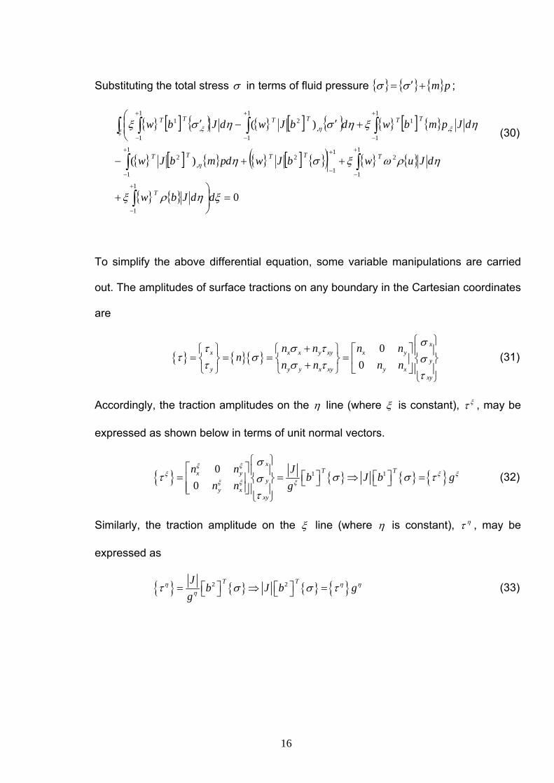
Substituting the total stress σ in terms of fluid pressure { } { } { }pm+′= σσ ;
{ } [ ] { } { } [ ] { } { } [ ] { }
{ } [ ] { } { } [ ] { }( ) { } { }
{ } { } 0
)(
)(
1
1
1
1
21
1
21
1,
2
1
1,
11
1,
21
1,
1
=⎟⎟⎠
⎞+
++−
+′−⎜⎜⎝
⎛′
∫
∫∫
∫∫∫ ∫
+
−
+
−
+
−
+
−
+
−
+
−
+
−
ξηρξ
ηρωξση
ηξησησξ
η
ξηξ ξ
ddJbw
dJuwbJwdpmbJw
dJpmbwdbJwdJbw
T
TTTTT
TTTTTT
(30)
To simplify the above differential equation, some variable manipulations are carried
out. The amplitudes of surface tractions on any boundary in the Cartesian coordinates
are
{ } { }{ }0
0
xx x x y xy x y
yy y y x xy y x
xy
n n n nn
n n n n
στ σ ττ σ στ σ τ
τ
⎧ ⎫+⎧ ⎫ ⎧ ⎫ ⎡ ⎤ ⎪ ⎪= = = =⎨ ⎬ ⎨ ⎬ ⎨ ⎬⎢ ⎥+⎩ ⎭ ⎩ ⎭ ⎣ ⎦ ⎪ ⎪
⎩ ⎭
(31)
Accordingly, the traction amplitudes on the η line (where ξ is constant), ξτ , may be
expressed as shown below in terms of unit normal vectors.
{ } { } { } { }1 100
xT Tx y
yy x
xy
n n Jb J b g
n n g
ξ ξξ ξ ξ
ξ ξ ξ
στ σ σ τσ
τ
⎧ ⎫⎡ ⎤ ⎪ ⎪ ⎡ ⎤ ⎡ ⎤= = ⇒ =⎢ ⎥ ⎨ ⎬ ⎣ ⎦ ⎣ ⎦⎢ ⎥ ⎪ ⎪⎣ ⎦
⎩ ⎭
(32)
Similarly, the traction amplitude on the ξ line (where η is constant), ητ , may be
expressed as
{ } { } { } { }2 2T TJ
b J b gg
η η ηητ σ σ τ⎡ ⎤ ⎡ ⎤= ⇒ =⎣ ⎦ ⎣ ⎦ (33)

17
Substituting the above simplification into the main differential equation of motion yields
{ } [ ] { } { } [ ] { }
{ } [ ] { } [ ] { } { } [ ] { } [ ] { }
{ } { }( ) { } { } { } { } 0(
))(())((
1
1
1
1
21
1
1
1
2,,
21
1
2,,
2
1
1,
11
1,
1
=⎟⎟⎠
⎞+++
+−′+−
+⎜⎜⎝
⎛′
∫∫
∫∫
∫∫ ∫
+
−
+
−
+
−
+
−
+
−
+
−
+
−
ξηρξηρωξτ
ηησ
ηξησξ
ηη
ηηηη
ξξ ξ
ddJbwdJuwgw
dpmbJwbJwdbJwbJw
dJpmbwdJbw
TTT
TTTTTTTT
TTTT
(34)
Furthermore, the derivative [ ]( )η,
2bJ is defined as
[ ]( )⎥⎥⎥
⎦
⎤
⎢⎢⎢
⎣
⎡
−−−=
ηη
η
η
η
,,
,
,
,2 0
0
yxx
ybJ
(35)
Comparing the above derivative with the [ ]( )1bJ results in [ ]( ) [ ]( )1,
2 bJbJ −=η
. Setting
the integrand of the integral over ξ to zero satisfies the above equation and
effectively enforces the main differential equation of motion exactly in the radial
direction. Furthermore, substituting the above equation (35) into equation (34) leads
to
{ } [ ] { } { } [ ] { }
{ } [ ] { } [ ] { } { } [ ] { } [ ] { }
{ } { }( ) { } { } { } { } 0
)()(
1
1
1
1
21
1
1
1
2,
11
1
2,
1
1
1,
11
1,
1
=+++
−+′−+
+′
∫∫
∫∫
∫∫
+
−
+
−
+
−
+
−
+
−
+
−
+
−
ηρξηρωξτ
ηησ
ηξζησξ
ηη
ηη
ξξ
dJbwdJuwgw
dJpmbwbwdJbwbw
dJpmbwddJbw
TTT
TTTTTTTT
TTTT
(36)
Substituting { } { } [ ]TuTT Nww = into the differential equation of motion (15) together with
the finite element displacements and pressure functions results equation (37).

18
{ } [ ] [ ] { } { } [ ] [ ] { }[ ]{ }
{ } [ ] [ ] [ ] [ ] { }
{ } [ ] [ ] [ ] [ ] { }[ ]{ } { } [ ] { }( )
{ } [ ] [ ]{ } { } [ ] { } 0)(
)()(
)(
)(
1
1
1
1
2
1
1
1
1
2,
1
1
1
2,
1
1
1,
11
1,
1
=++
+−+
′−+
+′
∫∫
∫
∫
∫∫
+
−
+
−
+
−
+
−
+
−
+
−
+
−
ηρξηξρξω
τηξ
ησ
ηξξησξ
ηηη
η
ξξ
dJbNwdJuNNw
gNwdJpNmbNbNw
dJbNbNw
dJpNmbNwdJbNw
TuTuTuT
TuTpTTuTTuT
TTuTTuT
pTTuTTTuT
(37)
Substituting the above expressions with [ ]1uB and [ ]2
uB , defined below, and multiplying
both sides of the equation by { }[ ] 1−Tw yields :
[ ] { } [ ] { }[ ]{ } [ ] [ ] { }
[ ] [ ] { }[ ]{ } [ ] { }( )
[ ] [ ]{ } [ ] { } 0)(
)()(
)()(
1
1
1
1
2
1
1
1
1
21
1
1
211
1,
11
1,
1
=++
+−+
′−++′
∫∫
∫
∫∫∫
+
−
+
−
+
−
+
−
+
−
+
−
+
−
ηρξηξρξω
τηξ
ησηξξησξ
ηη
ξξ
dJbNdJuNN
gNdJpNmBB
dJBBdJpNmBdJB
TuuTu
TupTu
Tu
Tu
Tu
pTu
Tu
(38)
Substituting the expressions for { }σ ′ and { }ξσ ,′ (equations 22 and 25 respectively)
yields
[ ] [ ] [ ]{ } [ ]{ } [ ]{ } [ ] { }[ ]{ }
[ ] [ ] { }[ ]{ } [ ] [ ] [ ] [ ]{ } [ ]{ }
[ ] { }( ) [ ] [ ]{ } [ ] { } 0)(
)(1)()()()(
)()(1)(1)(
1
1
1
1
21
1
1
1
2,
1211
1
21
1
1,
11
1
22,
2,
11
=+++
⎟⎟⎠
⎞⎜⎜⎝
⎛+−+−+
+⎟⎟⎠
⎞⎜⎜⎝
⎛−+
∫∫
∫∫
∫∫
+
−
+
−
+
−
+
−
+
−
+
−
+
−
ηρξηξρξωτ
ηξξ
ξηξ
ηξξηξξ
ξξ
ξξ
ηη
ξ
ξξξξ
dJbNdJuNNgN
dJuBuBDBBdJpNmBB
dJpNmBdJuBuBuBDB
TuuTuTu
uuT
uT
upT
uT
u
pTuuu
Tu
(39)
19
Further simplification and rearranging results in;
[ ] [ ][ ] { } [ ] { }[ ] { } [ ] [ ][ ] { }
[ ] [ ][ ] { } [ ] [ ][ ] { } [ ] [ ][ ] { }
[ ] [ ] { } [ ] { }[ ] [ ] { }[ ] { }
[ ] { } [ ] { }( ) 0
)()()(
)()()(
)()()(
1
1
1
1
2
1
1
211
1
22
1
1
22,
1
1
21,
1
1
12
,
1
1
11,
1
1
12,
1
1
112
=++
−++
−+−
++
+
−
+
−
+
−
+
−
+
−
+
−
+
−
+
−
+
−
+
−
∫
∫∫
∫∫∫
∫∫∫
ηη
ξξ
ξξξξ
τξηρξ
ξηξξηρξω
ξηξηξξηξ
ξηξξηξξηξ
gNdJbN
pdJNmBNmBudJNN
udJBDBudJBDBudJBDB
udJBDBpdJNmBudJBDB
TuTu
pTu
pTu
uTu
uT
uuT
uuT
u
uT
upT
uuT
u
(40)
The above derivation is valid for both the bounded and unbounded medium with the
integration limits between 10 →=ξ and ∞→=1ξ , respectively.
5.2 Weighted Residual Method Applied to the Continuity Equation
As with the equilibrium equation, the continuity equation is multiplied by a weighting
function and then integrated over the domain V. The weighting function { }TwP that is
multiplied by the differential equation of continuity is represented by the pore pressure
function { } ( ){ } ( )[ ] ( ){ }ξηηξ PPPP N, www == .
20
{ } { } [ ][ ] { } { } [ ][ ] { } [ ][ ] { }
[ ][ ] { } [ ][ ] { } [ ][ ] { } [ ][ ] { }
{ } { } [ ]{ } [ ]{ } { } { } [ ]{ } [ ]{ }
{ } 0
)1()1()(
))1111
11(
)
(
,2
,1
,2
,12
,,22
2,22
2,,12
,12
,21
2,21
,11
=+
+++++
++++
−+−∫
dVpKnwi
bbbbmwkububmwki
pmbbpmbbpmbbpmbb
pmbbpmbbmkpmbbmwk
f
T
TTf
TTf
TTTT
TTTTTT
V
ω
ξρ
ξρωω
ξξξξ
ξξ
ηξηξ
ηηηηξηξη
ηξηξξ
(41)
For the bounded/unbounded element, substituting ηξξ ddJdV = leads to
{ } { } [ ][ ] { } { } [ ][ ] { } [ ][ ] { }
[ ][ ] { } [ ][ ] { } [ ][ ] { } [ ][ ] { }
{ } { } [ ]{ } [ ]{ } { } { } [ ]{ } [ ]{ }
{ } 0)
)1()1()(
))1111
11((
)
(
,2
,1
,2
,12
,,22
2,22
2,,12
,12
,21
2,21
,11
1
1
=+
+++++
++++
−+−∫ ∫+
−
ξηω
ξρ
ξρωω
ξξξξ
ξξξ
ηξηξ
ηηηηξηξη
ηξηξξξ
ddJpKnwi
bbbbmwkububmwki
pmbbpmbbpmbbpmbb
pmbbpmbbmkpmbbmwk
f
T
TTf
TTf
TTTT
TTTTTT
(42)
Setting the integrand of the integral over ξ to zero satisfies the above equation and
effectively enforces the main differential equation of continuity in the radial direction.
{ } { } [ ][ ] { } { } { } [ ][ ] { }
{ } { } [ ][ ] { } { } { } [ ][ ] { }
{ } { } [ ][ ] { } { } { } [ ][ ] { }
{ } { } [ ][ ] { } { } { } [ ]{ }
{ } { } [ ]{ } { } { } [ ]{ } { } { } [ ]{ }
{ } 0
)1()1
)(()1
11
11
1(
,2
,1
,2
,12
,,22
2
,22
2,,12
,12
,21
2
,21
,11
1
1
)
(
=+
+++
+++
++
+−
+−∫+
−
ηω
ξρ
ξ
ρωωξ
ξξ
ξξ
ξξ
ηξη
ξηη
ηηξη
ξηη
ξηξξ
dJpKnwi
bbmwbbmwkubmw
ubmwkipmbbmw
pmbbmwpmbbmw
pmbbmwpmbbmw
pmbbmwpmbbmwk
f
T
TTTTf
TT
TTf
TTT
TTTTTT
TTTTTT
TTTTTT
(43)
21
This equation can be rewritten in the form (44). Substituting both the pore pressure
and displacement functions into the continuity equation leads to equation (45).
{ } { } [ ][ ] { } { } { } [ ][ ] { }
{ } { } [ ][ ] { } { } { } [ ][ ] { }
{ } { } [ ][ ] { } { } { } [ ][ ] { }
{ } { } [ ][ ] { } { } { } [ ]{ }
{ } { } [ ]{ } { } { } [ ]{ }
{ } { } [ ]{ } { } 0)
()
)((
1
1
2,
21
1
,1
1
1
2,
21
1
,1
1
1
22,,
221
1
,22
1
1,,
121
1
,12
1
1,
211
1
,21
1
1,
111
1
2
)
(
=++
++
+++
++
+−
+−
∫∫
∫∫
∫∫
∫∫
∫∫
∫∫
+
−
+
−
+
−
+
−
+
−
+
−
+
−
+
−
+
−
+
−
+
−
+
−
ηωξηξ
ηξρηξ
ηξρωωη
ηηξ
ηξη
ηξηξ
η
ξη
ξηη
ηηξη
ξηη
ξηξξ
dJpKnwidJbbmw
dJbbmwkdJubmw
dJubmwkidJpmbbmw
dJpmbbmwdJpmbbmw
dJpmbbmwdJpmbbmw
dJpmbbmwdJpmbbmwk
f
TTT
TTf
TT
TTf
TTT
TTTTTT
TTTTTT
TTTTTT
(44)
{ } { } [ ][ ] { }[ ] { } { } { } [ ][ ] { }[ ] { }
{ } { } [ ][ ] { }[ ] { } { } { } [ ][ ] { }[ ] { }
{ } { } [ ][ ] { }[ ] { } { } { } [ ][ ] { }[ ] { }
{ } { } [ ][ ] { }[ ] { } { } { } [ ][ ] { }
{ } { } [ ][ ] { } { } { } [ ]{ }
{ } { } [ ]{ } { } [ ] { } 0)()
())(
)()(()(
)()(
)()(
)()(
1
1
2,
21
1
,1
1
1
2,
21
1
,1
1
1
22,,
221
1
,22
1
1,,
121
1
,,12
1
1,
211
1
,,21
1
1,
111
1
2
)
(
=++
++
+++
++
+−
+−
∫∫
∫∫
∫∫
∫∫
∫∫
∫∫
+
−
+
−
+
−
+
−
+
−
+
−
+
−
+
−
+
−
+
−
+
−
+
−
ξηωξηξ
ηξρξηξ
ξηξρωωξη
ξηξηξ
ξηξξη
ξηξξηξ
η
ξη
ξηη
ηηξη
ξηη
ξηξξ
pdJNKnwidJbbmw
dJbbmwkudJNbmw
udJNbmwkipdJNmbbmw
pdJNmbbmwpdJNmbbmw
pdJNmbbmwpdJNmbbmw
pdJNmbbmwpdJNmbbmwk
p
f
TTT
TTf
uTT
uTTf
pTTT
pTTTpTTT
pTTTpTTT
pTTTpTTT
(45)
Rearranging results in ;

22
{ } { } [ ][ ] { }[ ] { } { } { } [ ][ ] { }[ ]
{ } { } [ ][ ] { }[ ] { } { } [ ][ ] { }[ ] { }
{ } { } [ ][ ] { }[ ] { } { } [ ][ ] { }[ ]
{ } { } [ ][ ] { }[ ] { }
{ } { } [ ][ ] { } { } { } [ ][ ] { }
{ } { } [ ]{ } { } { } [ ]{ }
{ } [ ] { } 0)(
)(
)()()((
)()
(
)()
()(
1
1
2
,2
1
1,
11
1
2
,2
1
1,
11
1
22
,,22
1
1
,22
1
1,
211
1
,,12
1
1,
121
1
,21
1
1,
111
1
2
)
(
=−
+−
++−
+
+−+
++
+
∫
∫∫
∫∫
∫
∫∫
∫∫
∫∫
+
−
+
−
+
−
+
−
+
−
+
−
+
−
+
−
+
−
+
−
+
−
+
−
ξηωξ
ηξηξρ
ξηξξηξρωω
ξη
ηη
ξηη
ηξξηξ
ηξ
ηξ
ηη
ηηη
ξηη
ηξξ
pdJNKnwi
dJbbmwdJbbmwk
udJNbmwudJNbmwki
pdJNmbbmw
dJNmbbmwdJNmbbmw
pdJNmbbmwdJNmbbmw
dJNmbbmwpdJNmbbmwk
p
f
T
TTTTf
uTTuTTf
pTTT
pTTTpTTT
pTTTpTTT
pTTTpTTT
(46)
Applying Green’s theorem to the surface integral leads to

23
{ } { } [ ][ ] { }[ ] { } { } { } [ ][ ] { }[ ]
{ } { } [ ][ ] { }[ ] { } { } [ ][ ] { }[ ]( )
{ } { } [ ][ ] { }[ ] { } { } [ ] [ ] { }[ ]
{ } { } [ ][ ] { }[ ] { } { } { } [ ][ ] { }[ ]
{ } { } [ ][ ] { }[ ] { } { } [ ][ ] { }[ ]( )
{ } { } [ ][ ] { }[ ] { } { } [ ] [ ] { }[ ]
{ } { } [ ][ ] { }[ ] { }
{ } { } [ ][ ] { } { } { } [ ][ ]( )
{ } { } [ ] [ ] { } { } [ ][ ] { } { } { } [ ]{ }
{ } { } [ ]{ }( ) { } { } [ ] { } { } { } [ ]{ }
{ } [ ] { } 0)(
)((
)()(
)(
)(
)(
1
1
2
2,
1
1,
21
1
1
1
2
,1
1
1
21
1
2,
1
1,
2
1
1
2,
11
1
22
,22
,
1
1
,2
,2
1
1,
221
1
1
1,
22,
221
1
,21
1
1,
12,
1
1
1,
21
1,
121
1
1
1
12,
121
1
,21
1
1,
111
1
2
)()
()
(
)
(
])
[
()
(
=−
−−+
−−−
++−
+
+−
++
−+−
−−
++
+
∫
∫∫
∫∫∫
∫
∫
∫∫
∫
∫∫
∫∫
∫
∫∫
+
−
+
−
+
−
+
−
+
−
+
−
+
−
+
−
+
−
+
−
+
−
+
−
+
−
+
−
+
−
+
−
+
−
+
−
+
−
+
−
+
−
+
−
ξηωξ
ηξηξξ
ηξρξηη
ξξηξρωω
ξη
ηη
η
ηξη
ηη
η
ηξξηξ
ηη
ξηη
ξ
ηη
ηηηη
ηηη
ηξη
ηη
η
ηξξ
pdJNKnwi
dJbbmwdJbbmwJbbmw
dJbbmwkudJNbmwdJNbmw
JNbmwudJNbmwki
pdJNmbbmw
dJNmbbmwdJNmbbmw
JNmbbmwdJNmbbmw
dJNmbbmwpdJNmbbmw
dJNmbbmwdJNmbbmw
JNmbbmwdJNmbbmw
dJNmbbmwpdJNmbbmwk
p
f
T
TTTTTT
TTf
uTTuTT
uTTuTTf
pTTT
pTTTpTTT
pTTTpTTT
pTTTpTTT
pTTTpTTT
pTTTpTTT
pTTTpTTT
(47)
Representing the weighting function { }w using the shape functions [ ])(ηpN in the
radial direction { })(ξw leads to
{ } [ ]{ } [ ]{ })()()(),( ξξηηξ wNwNw pp == (48)

24
where { } { } [ ]TpTT Nww )(ξ= and { } { } [ ]TpTT Nww ηη ξ ,, )(=
Substituting the above and grouping the relevant terms leads to equation (49).
{ } [ ] { } [ ] [ ] { }[ ] { }
[ ] { } [ ] [ ] { }[ ] [ ] { } [ ] [ ] { }[ ]( )
[ ] { } [ ] [ ] { }[ ] [ ] { } [ ] [ ] { }[ ] { }
[ ] { } [ ] [ ] { }[ ] [ ] { } [ ][ ] { }[ ]( )
[ ] { } [ ] [ ] { }[ ] [ ] { } [ ] [ ] { }[ ] { }
{ } [ ] { } [ ][ ] { } [ ] { } [ ][ ]( )
[ ] { } [ ] [ ] [ ] { } [ ][ ] { }
{ } [ ] { } [ ]{ } [ ] { } [ ]{ }( )
[ ] { } [ ] { } [ ] { } [ ]{ }
{ } [ ] [ ] { } 0)()(
)(
)(
)()()(
)(
)(
)()(
1
1
2
2,
1
1,
21
1
1
1
2,
11
1
2
1
1
2,
1
1,
2
1
1
2,
11
1
22
,22
,
1
1,
2,
21
1
1
1,
22,
211
1
,12
,
1
1
1,
21
1
1
1
12,
211
1
,11
1
1
2
)(
)(
)
(
)
(
])[
(
)
(
=−
−−
+−
−−
++−
++−
+−+
−−
++
∫
∫∫
∫
∫∫
∫
∫∫
∫
∫∫
∫
∫
+
−
+
−
+
−
+
−
+
−
+
−
+
−
+
−
+
−
+
−
+
−
+
−
+
−
+
−
+
−
+
−
+
−
+
−
ξηξξω
ηξηξ
ξηξξρ
ξηη
ξξηξξρωω
ξηη
η
ξηη
ηξ
ξηξξ
ηη
ξ
ηη
ξ
ηηηη
ηη
ξηη
η
ξξ
pdJNKnNwi
dJbbmNdJbbmN
JbbmNdJbbmNwk
udJNbmNdJNbmN
JNbmNudJNbmNwki
pdJNmbkbmNdJNmbkbmN
JNmbbmNdJNmbkbmN
pdJNmbkbmNdJNmbkbmN
JNmbkbmNdJNmbkbmN
pdJNmbkbmNw
p
f
TpT
TTpTTp
TTpTTpTf
uTTpuTTp
uTTpuTTpTf
pTTTppTTTp
pTTTppTTTp
pTTTppTTTp
pTTTppTTTp
pTTTpT
(49)
Substituting [ ]( ) [ ]( )1,
2 bJbJ −=η
results in;
25
[ ] { } [ ] [ ] { }[ ] { } [ ] { } [ ] [ ] { }[ ]
[ ] { } [ ] [ ] { }[ ]( ) [ ] { } [ ] [ ] { }[ ]
[ ] { } [ ] [ ] { }[ ] { } [ ] { } [ ] [ ] { }[ ]
[ ] { } [ ] [ ] { }[ ]( ) [ ] { } [ ] [ ] { }[ ]
[ ] { } [ ] [ ] { }[ ] { } [ ] { } [ ][ ] { }
[ ] { } [ ][ ]( ) [ ] { } [ ][ ] [ ] { } [ ][ ] { }
[ ] { } [ ]{ } [ ] { } [ ]{ }( )
[ ] { } [ ]{ } [ ] { } [ ]{ } [ ] [ ] { } 0)(
)(
)()()(
)(
)(
1
1
22,
1
1
11
1
1
1
2,
11
1
2
1
1
2,
1
1
11
1
2
,1
1
1
22,
22,
1
1
,21
1
1
1
1,
22
,21
1
1,
12,
1
1
111
1
1
1
12
,21
1
1,
111
1
2
)
(
)(
])
[
()
(
)(
=−−+
+−
−++
+−+
−−+
−+−
++
+
∫∫∫
∫
∫∫
∫∫
∫
∫∫
∫
∫∫
+
−
+
−
+
−
+
−
+
−
+
−
+
−
+
−
+
−
+
−
+
−
+
−
+
−
+
−
+
−
+
−
+
−
+
−
ξηωξηξηξ
ξηξρ
ξηηξ
ξηξρωωξη
η
ηξη
η
ηξξηξ
η
ξ
η
ξηη
ηη
ηξη
ηξξ
pdJNKnNidJbbmNdJbbmN
JbbmNdJbbmNk
udJNbmNdJNbmNJNbmN
udJNbmNkipdJNmbkbmN
dJNmbkbmNJNmbkbmN
dJNmbkbmNpdJNmbkbmN
dJNmbkbmNJNmbkbmN
dJNmbkbmNpdJNmbkbmN
p
f
TpTTpTTp
TTpTTpf
uTTpuTTpuTTp
uTTpf
pTTTp
pTTTppTTTp
pTTTppTTTp
pTTTppTTTp
pTTTppTTTp
(50)
The above equation may be rewritten in the form of equation 51.
[ ] [ ] { } [ ] [ ]( ) [ ] [ ] [ ] [ ]
[ ] [ ] { } [ ] [ ]( ) [ ] [ ] { }
[ ] { } [ ] { } [ ] { } [ ]
[ ] [ ] [ ] [ ]( ) { } [ ] { } [ ] { }
[ ] { } [ ] { }( ) [ ] [ ] { } 0)(
)(
)()()(
)()(
)(
1
1
21
1
221
1
11
1,
11
1
21
1
21
1
2
1
1
12,
11
1
22
221
1
1
1
22,
211
1
121
1
111
1
1
1
12,
111
1
2
)
()
(
)()
(
=−+−
+−+−
+−+−
−++
−++
∫∫
∫∫∫
∫∫
∫∫
∫∫∫
+
−
+
−
+
−
+
−
+
−
+
−
+
−
+
−
+
−
+
−
+
−
+
−
+
−
+
−
+
−
+
−
ξηωξξηξ
ηξηξρξη
ηξρωωξηξρωω
ξηξζη
ηηξξηξ
ξ
ξ
ξ
ξξ
pdJNKnNiJbBdJbB
dJbBdJbBkuJNBdJNB
dJBmNkiudJBmNki
pdJBkBJBkBpddJBkB
dJBkBdJBkBJBkBpdJBkB
p
f
TpTAp
Tp
Tp
Tpf
uTAp
uTp
uTTp
fuTTp
f
pT
ppTA
ppT
p
pT
ppT
ppTA
ppT
p
(51)

26
where
[ ] [ ] { }[ ] [ ] { }[ ]pTpTp NmbNmbB 111 )( == η ,
[ ] [ ] { }[ ] [ ] { }[ ] ηηζη ,2
,22 ),( pTpT
p NmbNmbB == .
[ ] [ ] { } [ ] [ ] { } [ ]222 ),( bmNbmNB TTpTTpTAp == ζη
[ ] [ ][ ] [ ][ ]uuu NbNbB 111 )( == η
[ ] [ ][ ] [ ][ ]ηηη ,2
,22 )( uu
u NbNbB ==
6. Summary of the Finite Element Coupled Consolidation Equations
The final formulation of the finite element equations (40) and (51) may be re-written in
the following compact form:
[ ] { } [ ] [ ] [ ] { } [ ]{ } [ ] { } [ ] { }[ ] [ ] { } { } { } 0)()()()(
)()()()()()(243
,232022
,110
,20
=++−+
++−+−+
ξξξξξξ
ξξξξωξξξξξ ξξξξ
tb
T
FFpEE
pEuMuEuEEEuE (52)
[ ] { } [ ] [ ] [ ] { } { } [ ] { } { } [ ] { }[ ] { } [ ] [ ] { } { } { }
{ } { } { } 0)()()(
)()()()()(
)()()()(
)()(
)()(
432
123432,
232
2127,
1665,
25
=+−+
−+−+−+
−−+−+++−+
ξξξξξξ
ξξρξξρωωξξρωω
ξξωξξξξξ
ξ
ξξξ
bbb
bf
tPTf
Tf
ttT
FFF
FkuFEEkiuEki
pMipFEpFEEEpE
(53)
where
[ ] [ ] [ ][ ]∫+
−
=1
1
110 ηdJBDBE uT
u [ ] [ ] [ ][ ]∫
+
−
=1
1
121 ηdJBDBE uT
u [ ] [ ] [ ][ ]∫
+
−
=1
1
222 ηdJBDBE uT
u
[ ] [ ] { }[ ]∫+
−
=1
1
13 ηdJNmBE pTu
[ ] [ ] { }[ ]∫+
−
=1
1
24 ηdJNmBE pTu
[ ] [ ] [ ] ηdJNBE uTp
P ∫+
−
=1
1
24
[ ] [ ] [ ]∫+
−
=1
1
115 ηdJBkBE pT
p [ ] [ ] [ ]∫+
−
=1
1
126 ηdJBkBE pT
p [ ] [ ] [ ]∫
+
−
=1
1
227 ηdJBkBE pT
p

27
[ ] [ ] [ ]∫+
−
=1
1
0 ηρ dJNNM uTu [ ] [ ] [ ]∫+
−
=1
1
1 ηdJNKnNM p
f
Tp
{ } [ ] { }∫+
−
=1
1
)( ηρξ dJbNF Tub
{ } [ ] { }( ) 1
1)()(
+
−= ηη ξξ gtNF Tut { } [ ] [ ]( ) 1
1
121+
−= JBkBF p
TAp
t
{ } [ ] [ ]( ) 1
1
222+
−= JBkBF p
TAp
t { } [ ] [ ]( ) 1
123
+
−= JNBF uTA
pt { } [ ] { }∫
+
−
=1
1,
11 )( ηξ ξ dJbBF Tp
b
{ } [ ] { }∫+
−
=1
1
12 )( ηξ dJbBF Tp
b { } [ ] { }∫+
−
=1
1
23 )( ηξ dJbBF Tp
b { } [ ] { }( ) 1
1
24 )(+
−= JbBF TA
pb ξ
[ ] [ ][ ] [ ][ ]uuu NbNbB 111 )( == η
[ ] [ ][ ] [ ][ ]ηηη ,
2,
22 )( uuu NbNbB ==
[ ] [ ] { }[ ] [ ] { }[ ]pTpTp NmbNmbB 111 )( == η
[ ] [ ] { }[ ] [ ] { }[ ] ηηη ,
2,
22 )( pTpTp NmbNmbB ==
[ ] [ ] { } [ ] [ ] { } [ ]222 )( bmNbmNB TTpTTpTAp == η
7. Conclusion
A numerical formulation to correctly model the dynamic unbounded far-field boundary
for two-phase media in 2D has been developed. The method of analysis extends the
existing single-phase scaled boundary finite element method into a two-phase
coupled solid-fluid approach to produce a more realistic representation of saturated
soil at the unbounded far-field boundary. Body forces and surface tractions are
considered in the derivation. The concept of similarity, the compatibility equation and
Biot’s coupled consolidation equations have been used to derive the formulation for
the governing equations. The main difference from the single-phase version is the
presence of pore water pressures as additional parameters to be solved for, in
addition to the displacements, strain and stress. These are incorporated into the
static-stiffness matrices by producing fully coupled matrices. Solving the resulting
equations yields a boundary condition satisfying the far-field radiation condition
28
exactly. The coupled systems of differential equations are formulated for each
element (i.e. Eq. 52 and 53). These coupled systems are then solved to determine the
displacement and pore pressure functions in the radial direction. The computed
solutions are exact in a radial direction (perpendicular to the boundary and pointing
towards infinity), while converge to the exact solution in the finite element sense in the
circumferential direction parallel to the soil-structure boundary interface.
The major advantages gained over previous methods used to model dynamic soil-
structure interaction with coupled consolidation are :
• The computed solutions are exact in a radial direction (from the soil-structure
boundary pointing towards infinity), while converge to the exact solution in the finite
element sense in the circumferential direction parallel to the soil-structure boundary
interface.
• For the static case, the SBFEM results in symmetric dynamic-stiffness and unit-
impulse response matrices, which would not be the case if the BEM or FBEM were
used, making it much more efficient time- and storage-wise.
• The spatial discretisation of problems is reduced by one, e.g. for 2D problems,
1D surface finite elements are used to discretise the boundary, which result in
reducing the spatial dimension by one, and in turn the number of degrees of freedom
during the analysis.
• As with the boundary element method (BEM), by not discretising the domain,
internal displacements and stresses are computed more accurately than with the finite
element method (FEM). However, in contrast to the BEM, the behaviour of the
bounded near-field soil can be represented using any advanced constitutive model
(for example, based on plasticity). This is due to the SBFEM not requiring a
fundamental solution, which also eliminates the need to evaluate singular integrals

29
occurring in most fundamental solutions. Anisotropy can also be modelled using the
SBFEM without an increase in computational effort.
The effects of dynamic soil-structure interaction can be very pronounced. When
comparing the response of a structure embedded in soft ground to that of the same
structure founded on the surface of rigid rock, it is evident that (i) the presence of the
soil makes the dynamic system more flexible and (ii) the radiation of energy of the
propagating waves away from the structure, if occurring, increases the damping. If
seismic motion is applied at the base of the structure then the free-field motion will
differ from the bed-rock control motion; usually being amplified towards the free
surface. The excavation of the soil and insertion of a stiff base results in some
averaging of the translation plus a rotation of the foundation given horizontal
earthquake motion and the inertial loads resulting from the motion of the structure will
further modify the seismic motion along the base of the structure. The degree of this
interaction depends not only on the foundation stiffness, but also the stiffness and
mass properties of the structure and the nature of the applied excitation. Ignoring
dynamic soil-structure interaction effects could lead to a significantly over-
conservative design [18]. The coupled consolidation SBFEM formulation should
therefore be used for saturated soil where there is a flow of water, in order to
incorporate the effect of intermediate-term consolidation of soil under loads, which
would not be accounted for if the standard SBFEM was used.
Acknowledgements
The results presented in this paper were obtained in the course of research
sponsored by the British Engineering and Physical Sciences Research Council
(EPSRC) under Grant number GR/R 29833/01 to the first author at Loughborough
30
University. The authors gratefully acknowledge this support. The authors also
gratefully acknowledge Professor John Wolf’s support at EPFL in Switzerland.
References
[1] Lysmer J and Kuhlemeyer RL. Finite dynamic model for infinite media. ASCE J.
Eng. Mech. 1969; 95: 859-877.
[2] White W, Valliappan S and Lee, IK. Unified boundary for finite dynamic models.
ASCE J. Eng. Mech. 1977; 103: 949-964.
[3] Smith WD. A non-reflecting plain boundary for wave propagation problems. J.
Comput. Phys. 1974; 15.
[4] Bettess P and Zienkiewicz OC. Diffraction and refraction of surface waves using
finite and infinite elements. Int. J. Num. Meth. Eng. 1977; 11: 1271-1290.
[5] Chow YK and Smith IM. Static and periodic infinite solid elements. Int. J. Num.
Meth. Eng. 1981; 17: 503-526.
[6] Zhao C and Valliappan S. A dynamic infinite element for three dimensional
infinite domain wave problems. Int J. Num. Meth. Eng. 1992; 36.
[7] Simoni L and Schrefler B. Mapped infinite elements in soil consolidation. Int. J.
Num. Meth. Eng. 1987; 24.
[8] Khalili N, Valliappan S, Tabtabaie-Yazdi J and Yazdchi M. 1D infinite element for
dynamic problems in saturated porous media. Comm. Num. Meth. Eng. 1997; 13:
727-738; Khalili N, Yazdchi M and Valliappan S. Wave propagation analysis of two-
phase saturated porous media using coupled finite-infinite element method. Soil Dyn.
Earthq. Eng. 1999; 18: 533-553.
[9] Cheng AH-D and Liggett JA. Boundary integral equation method for linear
porous-elasticity with applications to soil consolidation. Int. J. Num. Meth. Eng. 1984;
20: 255-278.

31
[10] Cheng AH-D and Detournay E. A direct boundary element method for plane
strain poroelasticity. Int. J. Num. Anal. Meth. Geomech. 1988; 12: 551-572.
[11] Cleary MP. Fundamental solutions for a fluid saturated porous solid. Int. J.
Solids Struct. 1977; 13: 785-806.
[12] Dargush GF and Banerjee P. A new boundary element method for three-
dimensional coupled problems of consolidation and thermoelasticity. J. Appl. Mech.
1991; 58: 28-36.
[13] Bonnet G. Basic singular solutions for a poroelastic medium in the dynamic
range. J. Acoust. Soc. Am. 1987; 82: 1758-1762.
[14] Dominguez J. An integral formulation for dynamic poroelasticity. J. Applied
Mech. 1991; 58: 588-591.
[15] Yazdchi M, Khalili N and Valliappan S. Non-linear seismic behaviour of concrete
gravity dams using coupled finite element-boundary element method. Int. J. Num.
Meth. Eng. 1999; 44.
[16] Wolf JP and Song C. Dynamic-stiffness matrix in time domain of unbounded
medium by infinitesimal finite-element cell method. Earthq. Eng. Struct. Dyn. 1994;
23.
[17] Song C and Wolf J. The scaled boundary finite-element method - alias
consistent infinitesimal finite-element cell method for elastodynamics. Computer
Methods in Applied Mechanics and Engineering 1997; 147.
[18] Wolf JP. Foundation Vibration Analysis using Simple Physical Models: Prentice
Hall, 1994.
[19] Biot MA. General theory of three-dimensional consolidation. Journal of Applied
Physics 1941; 12: 155-164.