two-dimensional benchmark aerodynamic problems: a ... · parameterization process eliminates the...

American Institute of Aeronautics and Astronautics

1

Application of Direct and Surrogate-Based Optimization to

Two-Dimensional Benchmark Aerodynamic Problems: A

Comparative Study

Yonatan A. Tesfahunegn1 and Slawomir Koziel2

Engineering Optimization & Modeling Center, Reykjavik University, Menntavegur 1, 101 Reykjavik, Iceland

Joe-Ray Gramanzini3 and Serhat Hosder4 Missouri University of Science and Technology, Rolla, Missouri, 65409

Zhong-Hua Han5

Northwestern Polytechnic University, Xi’an, 710072, Shaanxi, China

and

Leifur Leifsson6

Iowa State University, Ames, Iowa, 50011

This paper presents the results of applying direct and surrogate-based optimization

(SBO) algorithms to two-dimensional aerodynamic benchmark problems, both involving

transonic flow, one invisvid and the other viscous. The direct optimization methods used in

this study are the adjoint-based FUN3D and Stanford University Unstructured solvers. The

SBO algorithms include the SurroOpt framework, which exploits approximation-based

models, the multi-level optimization (MLO) algorithm, which relies on physics-based models,

as well as the adjoint-enhanced MLO algorithm. The results demonstrate that direct

optimization and the approximation-based methods are able to yield designs that are

comparable to those obtained with high-dimensional shape parameterization methods.

Physics-based SBO shows a rapid design improvement at a low computational cost

compared to the direct and the approximation-based SBO techniques, which indicates

that—for certain problems—derivative-free methods may be competitive to adjoint-based

algorithms when embedded in surrogate-assisted frameworks. On the other hand, global

search approaches, while more expensive, exhibit the potential to produce the best quality

results.

I. Introduction

series of increasingly complex set of benchmark aerodynamic shape optimization problems has been

developed by the AIAA Applied Aerodynamics technical committee. The purpose is to establish realistic

benchmark problems which can be used to evaluate and test optimization techniques and shape parameterization

techniques. The benchmark problems include two-dimensional airfoil shapes and three-dimensional wing shapes

involving both inviscid and viscous flows. Single- and multi-point formulations are included with one or more

constraints. The problems have been solved by several groups in academia and industry and the first set of works1-9

was presented at the AIAA SciTech conference in 2014.

1 Post-doctoral Fellow, School of Science and Engineering. 2 Professor, School of Science and Engineering, Senior Member AIAA. 3 Graduate Student, Department of Mechanical and Aerospace Engineering, Student Member AIAA. 4 Associate Professor of Aerospace Engineering, Senior Member AIAA. 5 Professor, Department of Fluid Mechanics, School of Aeronautics, Member AIAA. 6 Assistant Professor, Department of Aerospace Engineering, 2271 Howe Hall, Senior Member AIAA.

ADow

nloa

ded

by N

ASA

LA

NG

LE

Y R

ESE

AR

CH

CE

NT

RE

on

Janu

ary

12, 2

015

| http

://ar

c.ai

aa.o

rg |

DO

I: 1

0.25

14/6

.201

5-02

65

53rd AIAA Aerospace Sciences Meeting

5-9 January 2015, Kissimmee, Florida

AIAA 2015-0265

Copyright © 2015 by the American Institute of Aeronautics and Astronautics, Inc. All rights reserved.

AIAA SciTech


2

This paper presents a comparative study of solving the two-dimensional benchmark problems using direct

optimization (see, e.g., Jameson10) and surrogate-based optimization (SBO) (see, e.g., Queipo et al.11, Forrester and

Keane12, and Koziel et al.13). The study was performed by three different research groups where each group has

different computational fluid dynamic (CFD) models, parameterization techniques, and optimization methods.

Direct optimization of the benchmark problems was performed using the adjoint-based FUN3D14 solver of the

NASA Langley Research Center, and the adjoint-based Stanford University Unstructured15 (SU2) solver. SBO of the

benchmark problems was performed using approximation-based models via the SurroOpt framework16 with an in-

house CFD solver, and using physics-based models via the Multi-Level Optimization (MLO) algorithm17 with the

FLUENT18 CFD solver, and the adjoint-enhanced MLO (AE-MLO) algorithm19 with SU2.

II. Methodology

In this section, we formulate the optimization problem and briefly describe the optimization algorithms, the CFD

models, and the design variables for each method.

A. Problem Formulation

The goal of aerodynamic shape optimization is to obtain a geometry that provides an optimum aerodynamic

performance, e.g., minimum drag for a given lift. We formulate the problem as a constrained nonlinear minimization

problem, i.e., for a given operating condition, solve

uxl

x

x

xx

≤≤

==

=≤

Nkh

Mjgts

f

k

j

,,1,0)(

,,1,0)(..

)(min

K

K

(1)

where f(x) is the objective function, x is the design variable vector, gj(x) are the inequality constraints, M is the number

of the inequality constraints, hk(x) are the equality constraints, N is the number of the equality constraints, and l and u

are the design variables lower and upper bounds, respectively.

B. Direct Optimization via FUN3D

1. Optimization Methodology

A gradient-based non-linear constraint optimization approach was used, which utilized the FUN3D14 solver of

NASA Langley Research Center to obtain the solution to flow field and discrete-adjoint equations. The design

sensitivity derivatives (the gradients) used in the optimization were obtained from the solution of adjoint equations.

For the adjoint-based design optimization procedure, a cost function is defined and augmented with the flow

equations and represented by the following Lagrangian equation20

��, �,�, Λ = ��,�,� + Λ ��,�, � (2)

Here, Λ is the flow field adjoint variable vector (the Lagrange multipliers), ��,�, � is the cost function, and

��,�, �, Λ is the Lagrangian function. D, Q, X, and R correspond to the vector of design variables, vector of

conserved variables, grid-point locations, and residual for a control volume respectively. The detailed derivation of

discrete flow field adjoint equations are given in Refs. 20 and 21.

The NPSOL22 code, which is based on a sequential quadratic programming (SQP) optimization algorithm was

implemented as the optimizer. In NPSOL, the search direction is computed from the solution of a Quadratic

Program (QP) sub-problem. Once the search direction is determined; the step length is computed by a Lagrangian

merit function. A quasi-Newton update is then used to update the Hessian of the Lagrangian and the process is

repeated until a local minimum is achieved. For more detail on the NPSOL algorithm, see Ref. 22.

2. Design Variables

NASA’s BandAids program23, which is based on a free-form shape deformation algorithm, was used to set up

the shape parameterization and the design variables utilized in the optimization process. The use of BandAids for the

parameterization process eliminates the need for the regeneration of a mesh. This technique also parameterizes the

Dow

nloa

ded

by N

ASA

LA

NG

LE

Y R

ESE

AR

CH

CE

NT

RE

on

Janu

ary

12, 2

015

| http

://ar

c.ai

aa.o

rg |

DO

I: 1

0.25

14/6

.201

5-02

65


3

shape perturbation rather than the geometry itself reducing the number of design variables23. The design variables

used in BandAids has no association with any aerodynamic geometric characteristics (such as camber and

thickness), rather the parameterization method uses the grid point and links it to the closest marking surface.

Throughout the optimization the grid is updated as following:

�� = �� + Δ�� (3)

where r is the grid point, v is the design variable vector (i.e., control points), rnb is the baseline grid, and ∆rn is the

perturbation of the shape. For details on the parameterization technique, see Ref. 23.

For the NACA 0012 case, a parametric study was conducted to determine the number of control points that

corresponded to the best optimal solution varying from 6 to 26 control points. In order to insure a symmetric airfoil

during the optimization process, the modified NACA 0012 had a single marking surface that lay on the entire outer

mold line (OML) of airfoil.

In addition to the number control points corresponding to the geometric design variables for the modified-NACA

0012, the angle of attack was also activated as a global design variable in the optimization process along with a lift

constraint to eliminate the occurrence of non-unique solutions24. The angle of attack (in degrees) was bounded with

[-0.001, 0.001] and the lift value was bounded with the interval [-0.001, 0.001].

3. CFD Model

The computational fluid dynamics simulation was implemented by using the Fully Unstructured Navier-Stokes

(FUN3D) code of NASA Langley Research Center. The FUN3D is a node-based solver which uses a second-order

upwind scheme and finite volume discretization14. For inviscid simulations, FUN3D solves a non-dimensional

formulation of the Euler equations. For the inviscid flow solution, the Van Leer inviscid flux construction method

was used with the Van Leer heuristic pressure limiter in the current study. This limiter was chosen due to the

capability of freezing the limiter in both the flow and adjoint solver to accelerate the convergence of the residuals.

The limiter was set to freeze at 1,500 iterations in both solvers. For each grid level a convergence accuracy of

machine zero was achieved within 3,300 iterations.

The inviscid grids for the modified NACA 0012 were created by using a hyperbolic C-mesh generator25. A grid

convergence study was conducted to provide grid independent results, which utilized 4 grid levels (see Appendix for

the results). Since FUN3D is an unstructured solver the structured grids where edited and diagonalized with the use

of Pointwise Meshing Software. The baseline mesh (grid level 2) used in the optimization consisted of an initial grid

size of 501 x 101 x 2 before diagonalization. The final grid consisted of 100,000 cells with 50,500 x 2 grid points

after the diagonalization. The NACA 0012 consisted of 400 grid points on the surface, with a wall spacing of 0.002

grid units. The farfield was set at 20 chord lengths.

C. Direct Optimization via SU2


Due to the availability of adjoint technology10, it is possible to perform direct optimization of the high-fidelity

CFD model. Using this technology, which is implemented in SU2,15, the cost of obtaining the gradients is almost

equivalent to one flow solution for any number of design variables. Hence the high-fidelity model f is optimized

using the gradient-based trust-region algorithm exploiting adjoint sensitivities. More specifically, the problem (1) is

solved as an iterative process.

))((minarg )()1(

)()(xx

xx

jj sHjj δ≤−

+ = , (4)

where x(j), j = 0, 1, …, is a sequence of approximate solutions to (1) , whereas sk(j)(x) is a linear expansion of f(x) at

x(j) defined as

)()()()( )()()()( jjjj ffs xxxxx −⋅∇+= . (5)

Here, the gradient of the model f (applies separately for the drag and lift coefficient) is obtained by the adjoint

equation (see, e.g., Jameson10). The linear model (5) satisfies the zero- and first-order consistency conditions with

the function sk(j)(x) at x(j), i.e., sk

(j)(x(j)) = f(x(j)), and ∇sk(j)(x(j)) = ∇f(x(j)). Optimization of the linear model is

Dow

nloa

ded

by N

ASA

LA

NG

LE

Y R

ESE

AR

CH

CE

NT

RE

on

Janu

ary

12, 2

015

| http

://ar

c.ai

aa.o

rg |

DO

I: 1

0.25

14/6

.201

5-02

65


4

constrained to the vicinity of the current design defined as ||x – x(j)|| ≤ δ(j), with the trust region radius δ(j) adjusted

adaptively using standard trust region rules26.

2. Design Variables

The Hicks-Henne bump functions27 are used as the design variables. In this approach a baseline airfoil shape,

z(x)baseline, is deformed to yield a new airfoil shape, z(x). The new airfoil shape can be written as

)()()( xzxzxz baseline ∆+=

(6)

where

∑=

=∆N

n

nn xfxz1

)()( δ

(7)

is the total deformation with

( )ne

n xxf π3sin)( =

(8)

being the Hicks-Henne bump functions, δn is the deformation amplitude, N is the number of deformations, and

( )( )n

nx

e10

10

log

5.0log=

(9)

where xn ∈ [0,1] is the location of the function maximum. In airfoil shape optimization, the number of bumps, N,

and their locations of maxima, xn, are, typically, fixed. The designable parameters are then the amplitudes, δn, with

the design variable vector written as x = [δ1 δ2 ⋅⋅⋅ δN]T. We use N = 15 with the bumps equally spaced in xn

∈[0.05,0.95].

3. CFD Model

The Stanford University Unstructured15 (SU2) computer code is utilized for the inviscid fluid flow simulations.

The compressible Euler equations are solved with an implicit density-based formulation and the inviscid fluxes

calculated by an upwind-biased second-order spatially accurate Roe flux scheme. Asymptotic convergence to a

steady state solution is obtained in each case. The solution convergence criterion for the high-fidelity model is the

one that occurs first of the following: a reduction in all the residuals by six orders, or a maximum number of

iterations of 1,000.

The inviscid grids are generated using the hyperbolic C-mesh of Kinsey and Barth28. The farfield is set 100 chords

away from the airfoil surface. The grids have 630 points in the streamwise direction and 360 points in the direction normal

to the airfoil surface. The region behind the airfoil to the farfield contains 360 points. The grid points were clustered at the

trailing edge and the leading edge of the airfoil to give a minimum streamwise spacing of 0.001 × chord length. The

distance from the airfoil surface to the first node is 5⋅10−4 × chord length. The mesh has roughly 163,000 cells. A typical

evaluation time of the inviscid CFD simulation (including grid generation and the flow solution) is around 27 minutes.

D. Surrogate-Based Optimization with Approximation Models via SurroOpt


A SBO-type optimizer called SurroOpt16,29 is used to explore the global optimum of an airfoil design problem.

“SurroOpt” is a generic optimization framework which can be used to efficiently solve arbitrary single and multi-

objective (Pareto front), unconstrained and constrained optimization problems, assuming that the design space is

continuous and smooth. The flowchart of SurroOpt is shown in Fig. 1 (right). SurroOpt has built-in DoE methods

well suited for computer experiments, such as Lantin hypercube sampling (LHS), uniform design (UD), and Monte

Carlo design (MC). A variety of surrogate models are employed such as quadratic response surface model (PRSM),

kriging, gradient-enhanced kriging (GEK)30, hierarchical kriging (HK)31, radial-basis functions (RBFs). Five infill

sampling criteria and the dedicated constraint handling methods can be used, such as minimizing surrogate

prediction (MSP), expected improvement (EI), probability of improvement (PI), mean squared error (MSE), and

Dow

nloa

ded

by N

ASA

LA

NG

LE

Y R

ESE

AR

CH

CE

NT

RE

on

Janu

ary

12, 2

015

| http

://ar

c.ai

aa.o

rg |

DO

I: 1

0.25

14/6

.201

5-02

65


5

Figure 1. Framework of airfoil design via a SBO-type optimizer (left: the main loop of multi-round optimization; right:

the flowchart of “SurroOpt”)

lower confidence bounding (LCB). Note that in this study, LHS is used for selecting the initial sample points and the

EI method is used as an infill sampling criterion. Some highly matured optimization algorithms, such as Hooke and

Jeeves pattern search, BFGS (quasi Newton’s methods), sequential quadratic programming (SQP), single/multi

objective genetic Algorithms(GA), are employed to solve the sub-optimizations in which the cost function(s) and

state function(s) are evaluated by the surrogate models. SurroOpt are paralleled by MPI, which allows the user to

run the code with multiple cores (or processors) to speed up the optimization. SurroOpt has a user-defined interface,

with which the user can set up their own optimization problems. Note that a SBO-type optimizer has the feature that

one can conveniently restart the optimization when the process was terminated due to failure of code or manual

parameter changing.

Since there is no general hints for settings the design space and other parameters, a so called “multi-round

optimization strategy” is used. First, according to the baseline design(s), we set lower- and -upper limits of the

design space as well as other parameters by initial guess, and run the SBO optimization until it converges or

maximum number of iterations is reached; then the SBO optimization is run again, taking the optimum(s) of the

previous round as starting point(s) and adjusting the design space as well as other parameters, according to the

experience or lesson learned from the previous round; the whole process is repeated until no better design can be

found. Figure 1 (left) shows the framework of this method.

2. Design Variables

The airfoil is parameterized by the class-shape function transformation (CST) method32. The airfoil is defined as

1 2

12 TE

12

, LE TE0

( ) ( ) ( ) y

( ) (1 )

( ) ( ),S(0) 2 ,S(1) tan ,

NN

N NNN

p

i i pi

y x C x S x x

C x x x

S x A B x R yβ=

= ⋅ + ⋅∆

= −

= = = + ∆∑

(10)

where [0,1],x y∈ are normalized (by airfoil chord c ) chord-wise and vertical coordinates, respectively; LER , β

and TEy∆ are normalized leading-edge nose radius, boat-tail angle and trailing-edge thickness TEy∆ , respectively ;

12 ( )N

NC x represents the “class function” which is used to define general classed of geometries and for a typical round

nose and sharp aft end airfoil, one should set the class function exponents 1 0.5N = and 2 1.0N = ; ( )S x denotes the

“shape function” which is used to define specific shapes within the geometry class, with (0)S directly related to the

airfoil leading-edge nose radius LER and (1)S related to the boat-tail angle β and trailing-edge thickness TEy∆ .

Dow

nloa

ded

by N

ASA

LA

NG

LE

Y R

ESE

AR

CH

CE

NT

RE

on

Janu

ary

12, 2

015

| http

://ar

c.ai

aa.o

rg |

DO

I: 1

0.25

14/6

.201

5-02

65


6

The shape function, ( )S x , is represented by summing up of the Bernstein polynomials ,i pB , and their

coefficients iA serve as the design variables of our airfoil design problem. [ , ]iA ∈ −∞ ∞ can describe all the possible

smooth airfoils, which makes it well suited for global optimization. In actual airfoil shape optimization, due to the

limited computational budget, we use the following method to specify an appropriate design space: firstly we use

CST to fit the baseline airfoil and obtain ,i baseA ; then we define the design space as , ,[ , ]i i base i i base iA A Aδ δ∈ − + by

perturbation of the baseline airfoil with an appropriate step size iδ ( iδ can be adjusted during optimization process).

Note that the number of design variables is determined by the order of Bernstein polynomials determines, which is

prescribed by the user. For example, p = 4, 8, 16 will result in the number of design variables of 5, 9, 17 ( 1p + )

for symmetric airfoils and 9, 17, 33 ( 2 1p + ) for non-symmetric airfoils.

3. CFD Model

An in-house CFD code called “PMNS2D” is used to solve the compressible Euler or Reynolds-averaged Navier-

Stokes equations. Jameson’s central scheme is used for spatial descretization; for inviscid simulation Runge-Kutta is

used time integration, whereas for viscous simulation, LU-SGS method is used. Multigrid, local-time stepping and

variable-coefficient implicit residual smoothing are utilized to accelerate the solution converging to steady state.

Particularly for the benchmark test case 1 (inviscid simulation of a modified NACA 0012 airfoil in transonic flow),

single grid is used since the using of multigrid technique can frequently leads to non-zero lift at zero angle of attack;

enthalpy dumping technique is also used, which greatly improves the efficiency and robustness of CFD simulation

for case 1. For RANS simulations, Spalart-Allmaras turbulence model is used for turbulence closure.

The O-type grids for inviscid flow simulation are generated by solving elliptic equations, with very good uniformity

and orthogonality. The typical grids used for optimization have 320 points in the streamwise direction and 160 points in

the direction normal to the airfoil surface. The grid points were clustered at the trailing edge and the leading edge of the

airfoil to give a minimum streamwise spacing of 0.0005 × chord length; the normal spacing of the first grid line is around

0.0005 × chord length. The mesh has around 51,200 cells. During optimization, the farfield is set at 15 chord lengths.

The flow simulation is terminated after the density residual has dropped 6 orders in magnitude or the maximum number of

iteration of 5000 has been reached. A typical evaluation time of the inviscid CFD simulation (including grid generation

and the flow solution) is around 3 minutes for a typical personal computer.

The C-type grids for viscous flow simulation are generated using a special technique called

conformal transformation, which ensures very good uniformity and orthogonality. The typical grids used for

optimization have 512 points in the streamwise direction and 208 points in the direction normal to the airfoil surface. The

grid points were clustered at the trailing edge and the leading edge of the airfoil to give a minimum streamwise spacing of

0.0005 × chord length; the normal spacing of the first grid line away from the airfoil surface is set to ensure that it’s y+<1.

The mesh has around 107,328 cells. During optimization, the farfield is set at about 30 chord lengths. The flow

simulation is terminated after the density residual has dropped 5.5 orders in magnitude or the maximum number of

iteration of 10,000 has been reached. A typical evaluation time of the viscous CFD simulation (including grid generation

and the flow solution) is around 1 hour for a typical personal computer.

E. Multi-Level Optimization with Physics-Based Models


To accelerate the solution of (1), we exploit a multi-level solution approach developed by Koziel and Leifsson17.

The multi-level optimization (MLO) approach does not attempt to solve the original problem (1) directly, i.e., solve

))((minarg*xx

xfH= , (11)

where H is an objective function, here f(x) = [Cl.f(x) Cd.f(x) Af(x)]T. Instead the approach exploits a family of low-

fidelity models denoted as {ck}, k = 1, … , K, and a sequence of approximate solutions to (11) is generated, x(k), k =

0, 1, …, (x(0) is the initial design) as

))((minarg)1(xx

xk

k cH=+ , (12)

where ck(x) is the response of the kth low-fidelity model response given as ck(x)=[Cl.c.k(x) Cd.c.k(x) Ac(x)]T. All low-

fidelity models are evaluated by the same CFD solver as the one used for the high-fidelity model f. Discretization of

Dow

nloa

ded

by N

ASA

LA

NG

LE

Y R

ESE

AR

CH

CE

NT

RE

on

Janu

ary

12, 2

015

| http

://ar

c.ai

aa.o

rg |

DO

I: 1

0.25

14/6

.201

5-02

65


7

the model ck+1 is finer than that of the model ck, which results in an improved level of accuracy but also a longer

evaluation time. In practice, K = 3 or 4. The discretization density may be controlled by solver-dependent

parameters (e.g., the meshing parameters). To further speed up the analysis time of each low-fidelity model, one can

limit the number of flow solver iterations.

The MLO algorithm works as follows. Starting from the initial design x(0), the coarsest model c1 is optimized to

produce a first approximation of the high-fidelity model optimum, x(1). The vector x(1) is used as a starting point to

find the next approximation of the high-fidelity model optimum, x(2), which is obtained by optimizing the next

model, c2. The process continues until the optimum x(K) of the last low-fidelity model cK.

Having x(K), we evaluate the model cK at all perturbed designs around x(K), i.e., at xk(K) = [x1

(K)… xk(K) + sign(k)·dk …

xn(K)]T, k = –n, –n+1, …, n–1, n. We use the notation c(k) = cK(xk

(K)). This data is used to refine the final design without

directly optimizing the high-fidelity model f. More specifically, we set up an approximation model involving c(k) and

optimize it in the neighborhood of x(K) defined as [x(K) – d, x(K) + d], where d = [d1 d2 … dn]T. The size of the

neighborhood can be selected based on sensitivity analysis of c1 (the cheapest of the low-fidelity models); usually d

equals 2 to 5 percent of x(K).

Here, approximation is performed using a reduced quadratic model q(x) = [q1 q2 … qm]T, defined as

2

2.

2

11..11.0.1 )]([)( nnjnjnnjjj

T

njj xxxxxxqq λλλλλ ++++++== + KKKx , (13)

The coefficients λj.r, j = 1, …, m, r = 0, 1, …, 2n, are uniquely obtained by solving appropriate regression problems.

In order to account for unavoidable misalignment between cK and f, instead of optimizing the quadratic model q, it

is recommended to optimize a corrected model q(x) + [f(x(K)) – cK(x(K))] that ensures a zero-order consistency

between cK and f. The refined design is then found as

)])()([)((minarg )()(*

)()(

K

k

K

dd

cfqHKK

xxxxxxx

−+=+≤≤−

, (14)

If necessary, step (14) can be performed a few times starting from a refined design, i.e., x* = argmin{x(K) – d ≤ x

≤ x(K) + d : H(q(x) + [f(x*) – cK(x*)])}. It should be noted that the high-fidelity model is not evaluated until executing

the refinement step (14). Also, each refinement iteration requires only a single evaluation of f.

The optimization procedure can be summarized as follows (where K is the number of models):

1. Set j = 1;

2. Select the initial design x(0);

3. Starting from x(j–1) find x(j) = arg min{x : H(cj(x))};

4. Set j = j + 1; if j < K go to 3;

5. Obtain a refined design according to (14).

2. Design Variables

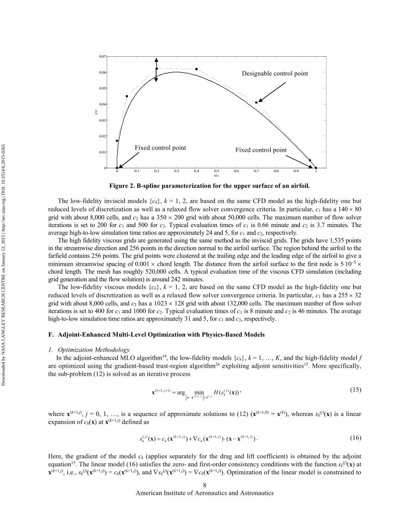
The airfoil is parameterized by a b-spline with six and eight control points for benchmark Case I and Case II,

respectively. The control points are used as design variables and allowed only to move freely vertically as shown in

Fig. 2 (in this figure we only show the upper surface of the airfoil). Each designable control point is free to move in

the vertical direction only.

3. CFD Model

For the MLO optimization methodology, we use the FLUENT18 flow solver for both the inviscid and the viscous

cases. The compressible Euler equations are solved for the inviscid cases, and for the viscous cases, we solve the

compressible RANS equations with the Spalart-Allmaras turbulence model. An implicit density-based formulation is

used and the inviscid fluxes are calculated by an upwind-biased second-order spatially accurate Roe flux scheme.

Asymptotic convergence to a steady state solution is obtained in each case. The solution convergence criterion for

the high-fidelity model is the one that occurs first of the following: a reduction in all the residuals by six orders, or a

maximum number of iterations of 1,200 and 1,800 for inviscid and viscous models, respectively.

The high fidelity inviscid grids are generated as described in Section II.C.3. A typical evaluation time of the inviscid

CFD simulation (including grid generation and the flow solution) is 15.8 minutes.

Dow

nloa

ded

by N

ASA

LA

NG

LE

Y R

ESE

AR

CH

CE

NT

RE

on

Janu

ary

12, 2

015

| http

://ar

c.ai

aa.o

rg |

DO

I: 1

0.25

14/6

.201

5-02

65


8

Figure 2. B-spline parameterization for the upper surface of an airfoil.

The low-fidelity inviscid models {ck}, k = 1, 2, are based on the same CFD model as the high-fidelity one but

reduced levels of discretization as well as a relaxed flow solver convergence criteria. In particular, c1 has a 140 × 80

grid with about 8,000 cells, and c2 has a 350 × 200 grid with about 50,000 cells. The maximum number of flow solver

iterations is set to 200 for c1 and 500 for c2. Typical evaluation times of c1 is 0.66 minute and c2 is 3.7 minutes. The

average high-to-low simulation time ratios are approximately 24 and 5, for c1 and c2, respectively.

The high fidelity viscous grids are generated using the same method as the inviscid grids. The grids have 1,535 points

in the streamwise direction and 256 points in the direction normal to the airfoil surface. The region behind the airfoil to the

farfield contains 256 points. The grid points were clustered at the trailing edge and the leading edge of the airfoil to give a

minimum streamwise spacing of 0.001 × chord length. The distance from the airfoil surface to the first node is 5⋅10−5 ×

chord length. The mesh has roughly 520,000 cells. A typical evaluation time of the viscous CFD simulation (including

grid generation and the flow solution) is around 242 minutes.

The low-fidelity viscous models {ck}, k = 1, 2, are based on the same CFD model as the high-fidelity one but

reduced levels of discretization as well as a relaxed flow solver convergence criteria. In particular, c1 has a 255 × 32

grid with about 8,000 cells, and c2 has a 1023 × 128 grid with about 132,000 cells. The maximum number of flow solver

iterations is set to 400 for c1 and 1000 for c2. Typical evaluation times of c1 is 8 minute and c2 is 46 minutes. The average

high-to-low simulation time ratios are approximately 31 and 5, for c1 and c2, respectively.

F. Adjoint-Enhanced Multi-Level Optimization with Physics-Based Models


In the adjoint-enhanced MLO algorithm19, the low-fidelity models {ck}, k = 1, …, K, and the high-fidelity model f

are optimized using the gradient-based trust-region algorithm26 exploiting adjoint sensitivities15. More specifically,

the sub-problem (12) is solved as an iterative process

))((minarg )()1,1(

)(),1(xx

xx

j

k

jk sHjjk δ≤−

++

+= , (15)

where x(k+1,j), j = 0, 1, …, is a sequence of approximate solutions to (12) (x(k+1,0) = x(k)), whereas sk(j)(x) is a linear

expansion of ck(x) at x(k+1,j) defined as

)()()()(),1(),1(),1()( jkjk

k

jk

k

j

k ccs+++ −⋅∇+= xxxxx . (16)

Here, the gradient of the model ck (applies separately for the drag and lift coefficient) is obtained by the adjoint

equation15. The linear model (16) satisfies the zero- and first-order consistency conditions with the function sk(j)(x) at

x(k+1,j), i.e., sk(j)(x(k+1,j)) = ck(x(k+1,j)), and ∇sk

(j)(x(k+1,j)) = ∇ck(x(k+1,j)). Optimization of the linear model is constrained to

0 0.1 0.2 0.3 0.4 0.5 0.6 0.7 0.8 0.9 10

0.01

0.02

0.03

0.04

0.05

0.06

0.07

x/c

z/c

Designable control point

Fixed control point Fixed control point

Dow

nloa

ded

by N

ASA

LA

NG

LE

Y R

ESE

AR

CH

CE

NT

RE

on

Janu

ary

12, 2

015

| http

://ar

c.ai

aa.o

rg |

DO

I: 1

0.25

14/6

.201

5-02

65


9

the vicinity of the current design defined as ||x – x(k+1.j)|| ≤ δ(j), with the trust region radius δ(j) adjusted adaptively

using standard trust region rules26.

The optimization procedure can be summarized as follows (where K is the number of models):

1. Set k = 1;

2. Select the initial design x(0);

3. Starting from x(k), find x(k+1) = arg min{x: H(ck(x))} as in (12) and using (15) and (16);

4. Set k = k + 1; if k < K go to 3; else END

Termination condition for the inner optimization loop (Step 3) is (||x(k+1,j+1) − x(k+1,j)|| < εk,1) , trust region radius

(δ(j) < εk,2) , and objective function resolution (||H(sk(j)(x(k+1,j+1))) − H(sk

(j)(x(k+1,j)))|| < εk,3) to terminate the gradient

based algorithm (15), where εk,i are tolerances for the respective termination conditions.

For lift constraint problems, the angle of attack is used as a dummy variable to find the target lift coefficient

value, and the optimization is performed at a fixed lift coefficient. In this case, Step 3 is modified and the angle of

attack is found by the modified secant method15 at the design x(k) before obtaining design x(k+1).

2. Design Variables

The Hick-Henne bump functions27, as described in Section II.C.2, are used as design variables.

3. CFD Models

The high-fidelity model f is based on the CFD simulations from SU2 as described in Section II.C.1. The low-

fidelity models are the same as the low fidelity models for the inviscid case as explained in Section II.E.3.

III. Benchmark Case I: Drag Minimization of the NACA 0012 in Transonic Inviscid Flow

A. Problem Statement

The objective is to minimize the drag coefficient (Cd) of modified NACA 0012 airfoil section at a free-stream Mach

number of M∞ = 0.85 and an angle of attack α = 0 deg. subject to a minimum thickness constraint. The optimization

problem is stated as

dCuxl ≤≤

min

(17)

where x is the vector of design variables, and l and u are the lower and upper bounds, respectively. The thickness

constraint is stated as

baselinexzxz )()( ≥

(18)

where z(x) is the airfoil thickness, x ∈ [0,1] is the chord-wise location, and z(x)baseline is the thickness of the baseline airfoil,

which is a modified version of the NACA 0012, defined as

( )432 1036.02843.03516.01260.02969.06.0)( xxxxxxz baseline −+−−±=

(19)

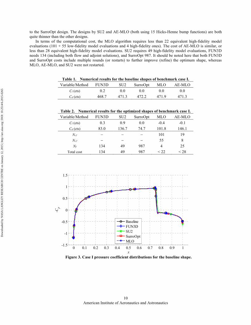
B. Results

Numerical results for each method for the baseline shape are shown in Table 1. The lift coefficient values are all

approximately 0.0 cts (1 lift count = 0.01), whereas the drag coefficient values differ at most by 3.5 cts (1 drag count

= 0.0001) with ranging from 468.7 cts (FUN3D) to 472.2 cts (SurroOpt). Here, SU2 and AE-MLO both use the SU2

flow solver, and MLO uses the FLUENT flow solver. The discrepancy could be because of flow solver differences,

but also due to slight differences in the grid geometries. Figure 3 shows the pressure distributions for each method

for the baseline design. They differ mainly in the shock strength and location.

Numerical results for the optimized designs are given in Table 2. The airfoil shapes are shown in Fig. 4, and the

pressure coefficient distributions are shown in Fig. 5. In terms of the drag coefficient values, the design obtained by

SurroOpt has the lowest value of 74.7 cts, the design by FUN3D has 83.0 cts, MLO design has 101.8 cts, SU2

design has 136.7 cts, and AE-MLO has 146.1 cts. The design by SurroOpt has a lift coefficient value of 0.0 cts,

whereas the other designs have non-zero lift coefficient values, although all are less than a count from the 0.0 value.

Comparing the shapes we notice that the design by FUN3D (20 design variables) has the fullest leading edge

shape (forward of 10% chord), whereas the SurroOpt design (17 design variables) has the fullest trailing edge shape

(behind 30% chord). The design by FUN3D is the thinnest one. The MLO design (6 b-spline variables) is quite close

Dow

nloa

ded

by N

ASA

LA

NG

LE

Y R

ESE

AR

CH

CE

NT

RE

on

Janu

ary

12, 2

015

| http

://ar

c.ai

aa.o

rg |

DO

I: 1

0.25

14/6

.201

5-02

65


10

to the SurroOpt design. The designs by SU2 and AE-MLO (both using 15 Hicks-Henne bump functions) are both

quite thinner than the other designs.

In terms of the computational cost, the MLO algorithm requires less than 22 equivalent high-fidelity model

evaluations (101 + 55 low-fidelity model evaluations and 4 high-fidelity ones). The cost of AE-MLO is similar, or

less than 28 equivalent high-fidelity model evaluations. SU2 requires 49 high-fidelity model evaluations, FUN3D

needs 134 (including both flow and adjoint solutions), and SurroOpt 987. It should be noted here that both FUN3D

and SurroOpt costs include multiple rounds (or restarts) to further improve (refine) the optimum shape, whereas

MLO, AE-MLO, and SU2 were not restarted.

Table 1. Numerical results for the baseline shapes of benchmark case I.

Variable/Method FUN3D SU2 SurroOpt MLO AE-MLO

Cl (cts) 0.2 0.0 0.0 0.0 0.0

Cd (cts) 468.7 471.3 472.2 471.9 471.3

Table 2. Numerical results for the optimized shapes of benchmark case I.

Variable/Method FUN3D SU2 SurroOpt MLO AE-MLO

Cl (cts) 0.3 0.9 0.0 -0.4 -0.1

Cd (cts) 83.0 136.7 74.7 101.8 146.1

Nc1 − − − 101 19

Nc2 − − − 55 8

Nf 134 49 987 4 25

Total cost 134 49 987 < 22 < 28

Figure 3. Case I pressure coefficient distributions for the baseline shape.

0 0.1 0.2 0.3 0.4 0.5 0.6 0.7 0.8 0.9 1-1.5

-1

-0.5

0

0.5

1

1.5

x

-C

p

Baseline

FUN3D

SU2

SurroOpt

MLO

Dow

nloa

ded

by N

ASA

LA

NG

LE

Y R

ESE

AR

CH

CE

NT

RE

on

Janu

ary

12, 2

015

| http

://ar

c.ai

aa.o

rg |

DO

I: 1

0.25

14/6

.201

5-02

65


11

Figure 4. Case I baseline and optimized airfoil shapes.

Figure 5. Case I pressure coefficient distributions for the optimized shapes (including the baseline).

IV. Benchmark Case II: Drag Minimization of the RAE 2822 in Transonic Viscous Flow

A. Problem Statement

The objective is to minimize the drag coefficient (Cd) of the RAE 2822 at a free-stream Mach number of M∞ = 0.734,

lift coefficient of 0.824, and Reynolds number of 6.5 × 106 subject to an area and pitching moment constraint. The task is

to solve the following constrained optimization problem:

Solve

dCuxl ≤≤

min

(20)

subject to the constraints

Cl = 0.824 (21)

Cm ≥ −0.092 (22)

0 0.1 0.2 0.3 0.4 0.5 0.6 0.7 0.8 0.9 10

0.01

0.02

0.03

0.04

0.05

0.06

0.07

x

z

Baseline

FUN3D

SU2

SurroOpt

MLO

AE-MLO

0 0.1 0.2 0.3 0.4 0.5 0.6 0.7 0.8 0.9 1-1.5

-1

-0.5

0

0.5

1

1.5

x

-C

p

Baseline

FUN3D

SU2

SurroOpt

MLO

AE-MLO

Dow

nloa

ded

by N

ASA

LA

NG

LE

Y R

ESE

AR

CH

CE

NT

RE

on

Janu

ary

12, 2

015

| http

://ar

c.ai

aa.o

rg |

DO

I: 1

0.25

14/6

.201

5-02

65


12

A ≥ Abaseline (23)

where Cm is the moment coefficient and A is the non-dimensional airfoil cross-sectional area.

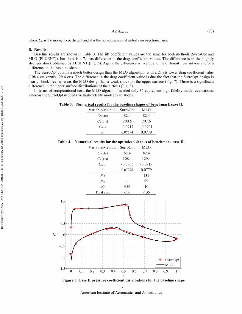
B. Results

Baseline results are shown in Table 3. The lift coefficient values are the same for both methods (SurroOpt and

MLO (FLUENT)), but there is a 7.1 cts difference in the drag coefficient values. The difference is in the slightly

stronger shock obtained by FLUENT (Fig. 6). Again, the difference is like due to the different flow solvers and/or a

difference in the baseline shape.

The SurroOpt obtains a much better design than the MLO algorithm, with a 21 cts lower drag coefficient value

(108.4 cts versus 129.4 cts). The difference in the drag coefficient value is due the fact that the SurroOpt design is

nearly shock-free, whereas the MLO design has a weak shock on the upper surface (Fig. 7). There is a significant

difference in the upper surface distributions of the airfoils (Fig. 8).

In terms of computational cost, the MLO algorithm needed only 35 equivalent high-fidelity model evaluations,

whereas the SurroOpt needed 656 high-fidelity model evaluations.

Table 3. Numerical results for the baseline shapes of benchmark case II.

Variable/Method SurroOpt MLO

Cl (cts) 82.4 82.4

Cd (cts) 200.5 207.6

Cm,c/4 -0.0917 -0.0901

A 0.07794 0.0779

Table 4. Numerical results for the optimized shapes of benchmark case II.

Variable/Method SurroOpt MLO

Cl (cts) 82.4 82.4

Cd (cts) 108.4 129.4

Cm,c/4 -0.0863 -0.0919

A 0.07796 0.0779

Nc1 − 139

Nc2 − 99

Nf 656 10

Total cost 656 < 35

Figure 6. Case II pressure coefficient distributions for the baseline shape.

0 0.1 0.2 0.3 0.4 0.5 0.6 0.7 0.8 0.9 1-1.5

-1

-0.5

0

0.5

1

1.5

x

-C

p

SurroOpt

MLO

Dow

nloa

ded

by N

ASA

LA

NG

LE

Y R

ESE

AR

CH

CE

NT

RE

on

Janu

ary

12, 2

015

| http

://ar

c.ai

aa.o

rg |

DO

I: 1

0.25

14/6

.201

5-02

65


13

Figure 7. Case II baseline and optimized airfoil shapes.

Figure 8. Case II pressure coefficient distributions for the optimized shapes (including the baseline).

V. Conclusion

In this work, the solution of the two benchmark aerodynamic optimization problems involving two-dimensional

transonic airfoil flow has been addressed. The problems were solved using direct and surrogate-based optimization (SBO)

techniques. The results show that direct optimization with adjoint sensitivities and SBO with approximation-based models

with high-dimensional shape parameterization are able to obtain comparable aerodynamic designs. The three groups of

methods, adjoint-based gradient search, physics-based surrogate-assisted optimization, and surrogate optimization with

approximation models, can be considered as three alternative approaches with their own advantages and disadvantages.

Adjoint-based methods are normally fast and simple to implement, however, they require the availability of adjoint

sensitivities. Physics-based SBO methods are capable to obtain a significant design improvement at a low computational

cost, however, require a careful setup of the underlying low-fidelity models, and computational benefits may be limited for

very high-dimensional problems when no sensitivity information is used. On the other hand, global methods (such as

surrogate-based search with approximation models) tend to yield very good solutions, but at a relatively high

computational cost. While the best choice of the method is normally problem dependent, the awareness of the merits and

weaknesses of particular techniques is the first step to make such a choice wisely.

0 0.1 0.2 0.3 0.4 0.5 0.6 0.7 0.8 0.9 1

-0.06

-0.04

-0.02

0

0.02

0.04

0.06

x

z

Baseline

SurroOpt

MLO

0 0.1 0.2 0.3 0.4 0.5 0.6 0.7 0.8 0.9 1-1.5

-1

-0.5

0

0.5

1

1.5

x

-C

p

Baseline

SurroOpt

MLO

Dow

nloa

ded

by N

ASA

LA

NG

LE

Y R

ESE

AR

CH

CE

NT

RE

on

Janu

ary

12, 2

015

| http

://ar

c.ai

aa.o

rg |

DO

I: 1

0.25

14/6

.201

5-02

65


14

Appendix

In the appendix we provide additional results from each optimization method for each benchmark case.

A. Benchmark Case I: Drag Minimization of the NACA 0012 in Transonic Inviscid Flow

1. Results from FUN3D

The optimization of the modified-NACA 0012 with baseline grid resulted in a drag reduction from 473.91 to

99.979 drag counts (a reduction of 377 drag counts) after 67 design iterations (Table 1). Each design iteration

required the solution of the flow field and the adjoint equations. The optimal results were obtained with 20 control

points (design variables). A grid convergence study was conducted with the optimal shape, resulting in a final drag

count of 82.966 with the finest grid level (grid level 4). The difference in drag between grid level 3 and grid level 4

was found to be less than 2 drag counts (Tables A.1 and A.2).

Table A.1. Grid convergence study for the initial shape with FUN3D.

Grid size Cl (cts) Cd (cts)

251 x 51 -40.62 493.827

501 × 101 1.06 473.91

1000 × 200 1.53 468.67

2000 × 400 38.15 467.81

Table A.2. Grid convergence study for the optimized shape with FUN3D.


251 x 51 4.16 156.26

501 × 101 10.38 99.979

1000 × 200 -2.55 82.967

2000 × 400 76.30 84.624

2. Results from SU2

Table A.3. Grid convergence study for the initial shape with SU2.


140 × 80 0.0 453.47

420 × 240 0.0 471.31

630 × 360 0.0 471.36

910 × 520 0.0 471.34

Table A.4. Grid convergence study for the optimized shape with SU2.


140 × 80 -25.90 350.46

420 × 240 -0.17 137.73

630 × 360 0.02 136.74

910 × 520 0.00 136.40

3. Results from SurroOpt

3.1 Optimization results

By using of a SBO-type optimizer, SurroOpt, the optimization is run in 7 rounds. Note that 17 design variables

(CST coefficients) and grids of 320×160 are used. The shape and the pressure distribution of the optimal airfoils for

different rounds of optimization are shown in Fig. A.1 and Fig. A.2, respectively; the corresponding force

coefficients are shown in Table A.5. We can see that the latter part of the optimal airfoils is much thicker than the

baseline airfoil, which leads to a relatively plain surface and is in favor of reducing the shock wave drag. Note that

Dow

nloa

ded

by N

ASA

LA

NG

LE

Y R

ESE

AR

CH

CE

NT

RE

on

Janu

ary

12, 2

015

| http

://ar

c.ai

aa.o

rg |

DO

I: 1

0.25

14/6

.201

5-02

65


15

there is a small bump existing in the chord-wise position of 0.6c to 0.7c of the optimal airfoil, which contributes to

control the strength of the shock near the trailing edge. From figure A.3, one can see that the drag coefficient can be

further reduced after each round of optimization, until a limit value is reached. Since the difference of drag

coefficients between the 6th and 7th rounds is smaller than 1 count, we terminated the whole process after 7-th round

of optimization. The comparison of Mach number contours for baseline and final optimized airfoils are shown in

figure A.4. It is clearly shown that the strongly shock wave on the NACA 0012 airfoil surface breaks into a attached

shock wave and a detached shock wave. Since the attached shock wave is much weaker, the shock wave drag is

greatly reduced.

Figure A.1 Shape of optimal airfoils in each round of optimization with 17 design variables.

Figure A.2 Pressure distribution of optimal airfoils in each round of optimization with 17 design variables.

Table A.5 Force coefficient of optimal airfoil in each round with 17 design variables

Variable Baseline 1st round

Opt.

2nd round

Opt.

3rd round

Opt.

4th round

Opt.

5th round

Opt.

6th round

Opt.

7th round

Opt.

(cts)lC 0.002 0.000 -0.010 0.028 -0.025 -0.065 0.000 0.011

(cts)dC 472.19 246.08 97.16 90.19 79.97 76.95 74.87 74.68

N_CFD / 185 144 189 156 106 126 81

x/c

y/c

0 0.1 0.2 0.3 0.4 0.5 0.6 0.7 0.8 0.9 10

0.01

0.02

0.03

0.04

0.05

0.06

0.07

NACA0012(17-Variables)

OPT_1

OPT_2

OPT_3

OPT_4

OPT_5

OPT_6

OPT_7

x/c

cp

0 0.1 0.2 0.3 0.4 0.5 0.6 0.7 0.8 0.9 1

-1.5

-1

-0.5

0

0.5

1

1.5

NACA0012(17-Variables)

OPT_1

OPT_2

OPT_3

OPT_4

OPT_5

OPT_6

OPT_7

Dow

nloa

ded

by N

ASA

LA

NG

LE

Y R

ESE

AR

CH

CE

NT

RE

on

Janu

ary

12, 2

015

| http

://ar

c.ai

aa.o

rg |

DO

I: 1

0.25

14/6

.201

5-02

65


16

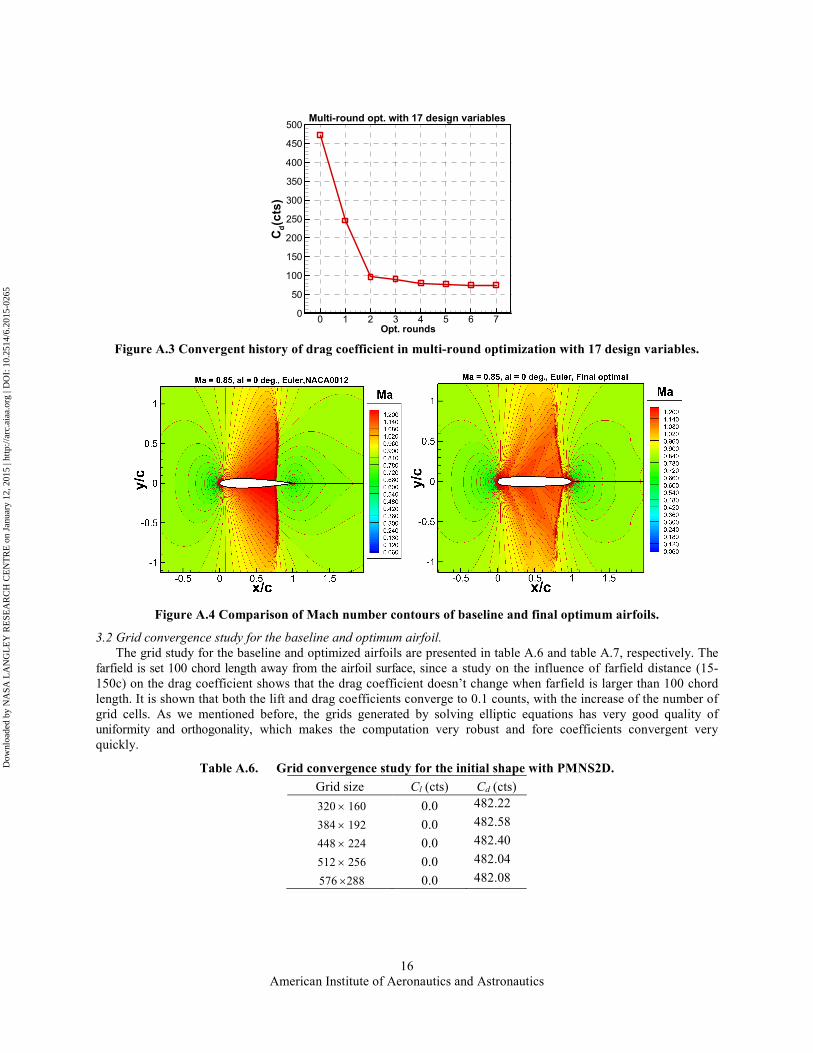
Figure A.3 Convergent history of drag coefficient in multi-round optimization with 17 design variables.

Figure A.4 Comparison of Mach number contours of baseline and final optimum airfoils.

3.2 Grid convergence study for the baseline and optimum airfoil.

The grid study for the baseline and optimized airfoils are presented in table A.6 and table A.7, respectively. The

farfield is set 100 chord length away from the airfoil surface, since a study on the influence of farfield distance (15-

150c) on the drag coefficient shows that the drag coefficient doesn’t change when farfield is larger than 100 chord

length. It is shown that both the lift and drag coefficients converge to 0.1 counts, with the increase of the number of

grid cells. As we mentioned before, the grids generated by solving elliptic equations has very good quality of

uniformity and orthogonality, which makes the computation very robust and fore coefficients convergent very

quickly.

Table A.6. Grid convergence study for the initial shape with PMNS2D.


320 × 160 0.0 482.22

384 × 192 0.0 482.58

448 × 224 0.0 482.40

512 × 256 0.0 482.04

576 ×288 0.0 482.08

Opt. rounds

Cd(cts)

0 1 2 3 4 5 6 70

50

100

150

200

250

300

350

400

450

500Multi-round opt. with 17 design variables

Dow

nloa

ded

by N

ASA

LA

NG

LE

Y R

ESE

AR

CH

CE

NT

RE

on

Janu

ary

12, 2

015

| http

://ar

c.ai

aa.o

rg |

DO

I: 1

0.25

14/6

.201

5-02

65


17

Table A.7. Grid convergence study for the optimized shape with PMNS2D.


320 × 160 0.0 83.00

384 × 192 0.0 79.40

448 × 224 0.0 77.50

512 × 256 0.0 76.69

576 ×288 0.0 76.73

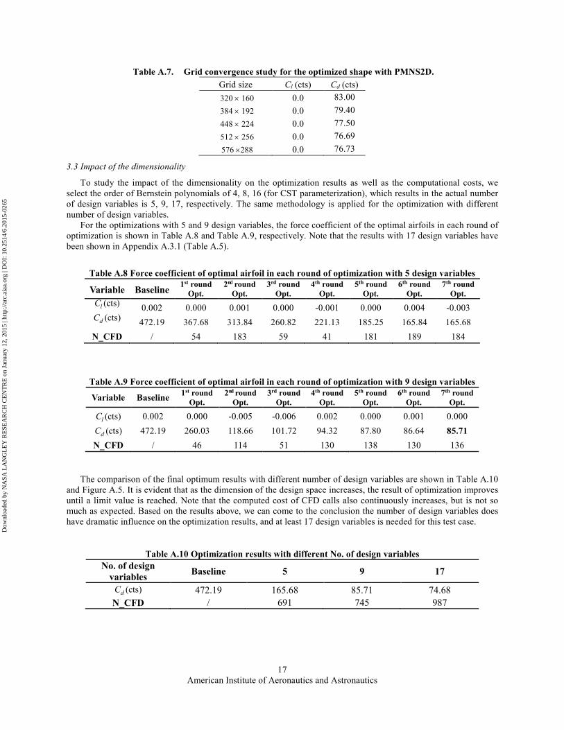
3.3 Impact of the dimensionality

To study the impact of the dimensionality on the optimization results as well as the computational costs, we

select the order of Bernstein polynomials of 4, 8, 16 (for CST parameterization), which results in the actual number

of design variables is 5, 9, 17, respectively. The same methodology is applied for the optimization with different

number of design variables.

For the optimizations with 5 and 9 design variables, the force coefficient of the optimal airfoils in each round of

optimization is shown in Table A.8 and Table A.9, respectively. Note that the results with 17 design variables have

been shown in Appendix A.3.1 (Table A.5).

Table A.8 Force coefficient of optimal airfoil in each round of optimization with 5 design variables


Opt.

2nd round

Opt.

3rd round

Opt.

4th round

Opt.

5th round

Opt.

6th round

Opt.

7th round

Opt. (cts)lC

0.002 0.000 0.001 0.000 -0.001 0.000 0.004 -0.003 (cts)dC

472.19 367.68 313.84 260.82 221.13 185.25 165.84 165.68

N_CFD / 54 183 59 41 181 189 184

Table A.9 Force coefficient of optimal airfoil in each round of optimization with 9 design variables


Opt.

2nd round

Opt.

3rd round

Opt.

4th round

Opt.

5th round

Opt.

6th round

Opt.

7th round

Opt.

(cts)lC 0.002 0.000 -0.005 -0.006 0.002 0.000 0.001 0.000

(cts)dC 472.19 260.03 118.66 101.72 94.32 87.80 86.64 85.71

N_CFD / 46 114 51 130 138 130 136

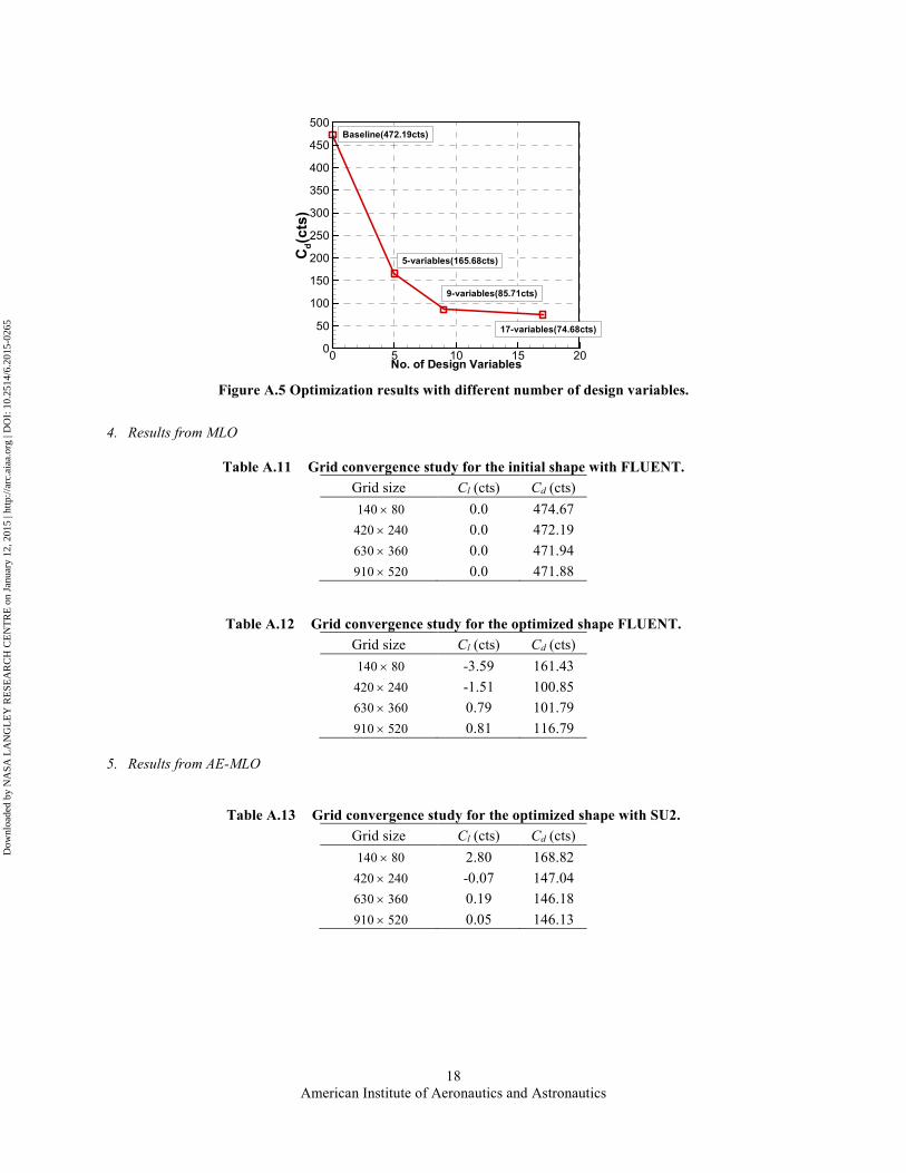
The comparison of the final optimum results with different number of design variables are shown in Table A.10

and Figure A.5. It is evident that as the dimension of the design space increases, the result of optimization improves

until a limit value is reached. Note that the computed cost of CFD calls also continuously increases, but is not so

much as expected. Based on the results above, we can come to the conclusion the number of design variables does

have dramatic influence on the optimization results, and at least 17 design variables is needed for this test case.

Table A.10 Optimization results with different No. of design variables

No. of design

variables Baseline 5 9 17

(cts)dC 472.19 165.68 85.71 74.68

N_CFD / 691 745 987

Dow

nloa

ded

by N

ASA

LA

NG

LE

Y R

ESE

AR

CH

CE

NT

RE

on

Janu

ary

12, 2

015

| http

://ar

c.ai

aa.o

rg |

DO

I: 1

0.25

14/6

.201

5-02

65


18

Figure A.5 Optimization results with different number of design variables.

4. Results from MLO

Table A.11 Grid convergence study for the initial shape with FLUENT.


140 × 80 0.0 474.67

420 × 240 0.0 472.19

630 × 360 0.0 471.94

910 × 520 0.0 471.88

Table A.12 Grid convergence study for the optimized shape FLUENT.


140 × 80 -3.59 161.43

420 × 240 -1.51 100.85

630 × 360 0.79 101.79

910 × 520 0.81 116.79

5. Results from AE-MLO

Table A.13 Grid convergence study for the optimized shape with SU2.


140 × 80 2.80 168.82

420 × 240 -0.07 147.04

630 × 360 0.19 146.18

910 × 520 0.05 146.13

No. of Design Variables

Cd(cts)

0 5 10 15 200

50

100

150

200

250

300

350

400

450

500

Baseline(472.19cts)

5-variables(165.68cts)



Dow

nloa

ded

by N

ASA

LA

NG

LE

Y R

ESE

AR

CH

CE

NT

RE

on

Janu

ary

12, 2

015

| http

://ar

c.ai

aa.o

rg |

DO

I: 1

0.25

14/6

.201

5-02

65


19

B. Benchmark Case II: Drag Minimization of the RAE 2822 in Transonic Viscous Flow

1. Results from MLO

Table B.1. Grid convergence study for the initial shape with FLUENT.

Grid size Cl (cts) Cd (cts) Cm,c/4

255 × 32 82.40 220.92 -0.087

511 × 64 82.40 211.43 -0.087

1023 × 128 82.41 208.49 -0.090

2047 × 256 82.40 207.43 -0.090

4095 × 512 82.40 208.35 -0.090

Table B.2. Grid convergence study for the optimized shape FLUENT.

Grid size Cl (cts) Cd (cts) Cm,c/4

255 × 32 82.41 142.47 -0.092

511 × 64 82.42 131.18 -0.090

1023 × 128 82.37 130.00 -0.092

2047 × 256 82.38 129.39 -0.092

4095 × 512 82.23 128.60 -0.090

Acknowledgments

Y. A. Tesfahunegn has received funding from the People Programme (Marie Curie Actions) of the European

Union's Seventh Framework Programme FP7/2007-2013/ under REA grant agreement n° PIEF-GA-2012-331454.

References 1Bisson, F., Nadarajah, S., and Shi-Dong, S., “Adjoint-Based Aerodynamic Optimization of Benchmark Problems,” AIAA 52nd

Aerospace Sciences Meeting, National Harbor, Maryland, January 13-17, 2014. 2Zhang, M., Wang, C., Rizzi, A., and Nangia, R., “Hybrid Feedback Design for Subsonic and Transonic Airfoils and Wings,” AIAA

52nd Aerospace Sciences Meeting, National Harbor, Maryland, January 13-17, 2014. 3Amoignon, O., Navaratil, J., and Hradil, J., “Study of Parameterizations in the Project CEDESA,” AIAA 52nd Aerospace Sciences

Meeting, National Harbor, Maryland, January 13-17, 2014. 4Poole, D.J., Allen, C.B., and Rendall, T.C.S., “Application of Control Point-Based Aerodynamic Shape Optimization to Two-

Dimensional Drag Minimization,” AIAA 52nd Aerospace Sciences Meeting, National Harbor, Maryland, January 13-17, 2014. 5 Telidetzki, K., Osusky, L., and Zingg, D.W., “Application of Jetstream to a Suite of Aerodynamic Shape Optimization Problems,”

AIAA 52nd Aerospace Sciences Meeting, National Harbor, Maryland, January 13-17, 2014. 6Carrier, G., Destarac, D., Meheut, M. Salah El Din, I., Peter, J., Ben Khelil, S., Brezillon, J., and Pestana, M. “Gradient-Based

Aerodynamic Optimization with the elsA Software,” AIAA 52nd Aerospace Sciences Meeting, National Harbor, Maryland, January 13-17,

2014. 7 Lyu, Z, Kenway, G.K.W., and Martins, J.R.R.A., “RANS-based Aerodynamic Shape Optimization Investigations of the Common

Research Model Wing,” AIAA 52nd Aerospace Sciences Meeting, National Harbor, Maryland, January 13-17, 2014. 8Epstein, B., Peigin, S., Bolsunovsky, A., and Timchenko, S., “Aerodynamic Shape Optimization by Automatic Hybrid Genetic Tool

OPTIMENGA_AERO,” AIAA 52nd Aerospace Sciences Meeting, National Harbor, Maryland, January 13-17, 2014. 9Leifsson, L., Koziel, S., Tesfahunegn, Y.A., Hosder, S., and Gramanzini, J.-R., “Aerodynamic Design Optimization: Physics-based

Surrogate Approaches for Airfoil and Wing Design,” AIAA 52nd Aerospace Sciences Meeting, National Harbor, Maryland, January 13-

17, 2014. 10Jameson, A., “Aerodynamic Design via Control Theory,” Journal of Scientific Computing, Vol. 3, 1988, pp. 233-260. 11N.V. Queipo, R.T. Haftka, W. Shyy, T. Goel, R. Vaidynathan, and P.K. Tucker, “Surrogate-based analysis and optimization,”

Progress in Aerospace Sciences, vol. 41, no. 1, pp. 1-28, Jan. 2005.

12A.I.J. Forrester and A.J. Keane, “Recent advances in surrogate-based optimization,” Prog. in Aerospace Sciences, vol. 45, no. 1-3,

pp. 50-79, Jan.-April, 2009. 13Koziel, S., Echeverría-Ciaurri, D., and Leifsson, L., “Surrogate-based methods,” in S. Koziel and X.S. Yang (Eds.) Computational

Optimization, Methods and Algorithms, Series: Studies in Computational Intelligence, Springer-Verlag, pp. 33-60, 2011. 14FUN3D Manual: 12.4 NASA/TM–2014–218179.

Dow

nloa

ded

by N

ASA

LA

NG

LE

Y R

ESE

AR

CH

CE

NT

RE

on

Janu

ary

12, 2

015

| http

://ar

c.ai

aa.o

rg |

DO

I: 1

0.25

14/6

.201

5-02

65


20

15Palacios, F., Colonno, M. R., Aranake, A. C., Campos, A., Copeland, S. R., Economon, T. D., Lonkar, A. K., Lukaczyk, T.

W., Taylor, T. W. R., and Alonso, J. J., “Stanford University Unstructured (SU2): An open-source integrated computational

environment for multi-physics simulation and design,” AIAA Paper 2013-0287, 51st AIAA Aerospace Sciences Meeting and

Exhibit, Grapevine, Texas, USA, 2013. 16Han, Z. -H, and Zhang, K. -S., Surrogate based optimization, Intec Book, Real-world Application of Genetic Algorithm, 2012, pp.

343-362. 17Koziel, S., and Leifsson, L., “Multi-Level Surrogate-Based Airfoil Shape Optimization,” 51st AIAA Aerospace Sciences

Meeting including the New Horizons Forum and Aerospace Exposition, Grapevine, Texas, January 7-10, 2013. 18FLUENT, ver. 14.5.7, ANSYS Inc., Southpointe, 275 Technology Drive, Canonsburg, PA 15317, 2013. 19Tesfahunegn, Y.A., Koziel, S., and Leifsson, L., “Surrogate-Based Airfoil Design with Multi-Level Optimization and

Adjoint Sensitivity,” 53rd AIAA Aerospace Sciences Meeting, Kissimmee, Florida, January 5-9, 2015. 20Nielsen, E.J., and Anderson, W.K., “Aerodynamic Design Optimization on Unstructured Meshes Using the Navier-Stokes

Equations,” AIAA Journal, Vol. 37, No. 11, 1999, pp. 1411-1419. 21FUN3D v12.4 Training Session 9: Adjoint-Based Design for Steady Flows, Eric J. Nielsen,

http://fun3d.larc.nasa.gov/session9_2014.pdf, March 2014. 22Gill, P.E., Murray, W., and Saunders, M.A., Wright, M.H., “Users Guide for NPSOL: A Fortran Package for Nonlinear

Programming, http://web.stanford.edu/group/SOL, December 2014. 23Samareh, J. A., “Aerodynamic Shape Optimization Based on Free-form Deformation,” 10th AIAA/ISSMO Multidisciplinary

Analysis and Optimization Conference, AIAA-2004-4630, Albany, New York, September 2004. 24Jameson, A., Vassberg, J.C., Ou, K., “Further studies of airfoils supporting non-unique solutions in transonic flow,” AIAA Journal

Vol. 50, No. 12, December 2012. 25Barth, T.J., Pulliam, T.H., and Buning, P.G., “Navier-Stokes Computations for Exotic Airfoils,” AIAA-85-0109, AIAA 23rd

Aerospace Sciences Meeting, Reno, NV, Jan. 1985. 26Conn, A.R., Gould, N.I.M., and Toint, P.L., Trust Region Methods, MPS-SIAM Series on Optimization, 2000. 27Hicks, R. M., and Henne, P. A., “Wing Design by Numerical Optimization,” Journal of Aircraft, Vol. 15, 1978, pp. 407–412. 28Kinsey, D. W., and Barth, T. J., “Description of a Hyperbolic Grid Generation Procedure for Arbitrary Two-Dimensional Bodies,”

AFWAL TM 84-191-FIMM, 1984. 29Liu, J., Han, Z. -H., and Song, W. -P., “Efficient kriging-based optimization design of transonic airfoils: some key issues,“ AIAA

Paper 2012-0967, 2012. 30Han, Z. -H., Görtz, S., and Zimmermann, R., “Improving Variable-Fidelity Surrogate Modeling via Gradient-Enhanced Kriging

and a Generalized Hybrid Bridge Function,” Aerospace Science and Technology, Vol. 25, No. 1 ,2013, pp. 177-189 31Han, Z. -H., and Görtz, S, “A Hierarchical Kriging Model for Variable-Fidelity Surrogate Modeling,” AIAA Journal, Vol.50, No.9,

2012, pp.1885-1896 32Kulfan, B. M., “Universal Parametric Geometry Representation Method,” Journal of Aircraft, Vol. 45, No. 1, 2008, pp. 142–158

Dow

nloa

ded

by N

ASA

LA

NG

LE

Y R

ESE

AR

CH

CE

NT

RE

on

Janu

ary

12, 2

015

| http

://ar

c.ai

aa.o

rg |

DO

I: 1

0.25

14/6

.201

5-02

65

two-dimensional benchmark aerodynamic problems: a ... · parameterization process eliminates the...

Documents