Twelfth Synthesis Imaging Workshop2010 June 8-15

Low Frequency InterferometryTracy Clarke (Naval Research Laboratory)

What is Low Frequency? Wikipedia: ‘Low frequency or low freq or LF refers to radio frequencies (RF) in the range of 30 kHz – 300 kHz.’

Not the definition normally used by radio astronomers.

Low freq radio astronomy = HF (3 MHz – 30 MHz), VHF (30 MHz – 300 MHz) and UHF (300 MHz – 3 GHz)

Ground-based instruments only reach to ~10 MHz due to ionosphere

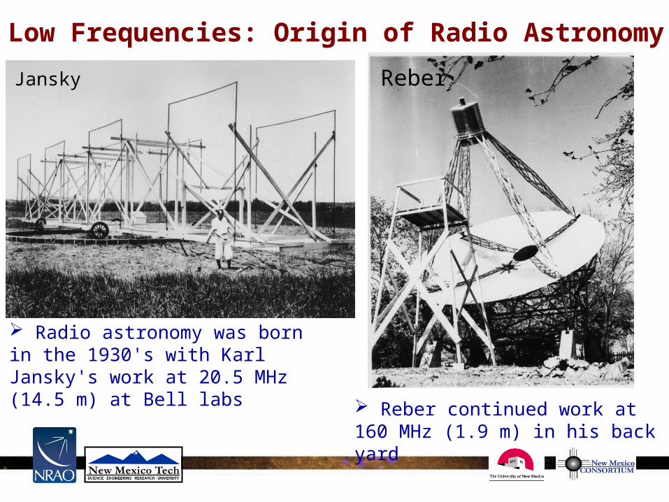
Low Frequencies: Origin of Radio Astronomy

Jansky

Radio astronomy was born in the 1930's with Karl Jansky's work at 20.5 MHz (14.5 m) at Bell labs

Reber continued work at 160 MHz (1.9 m) in his back yard

Reber

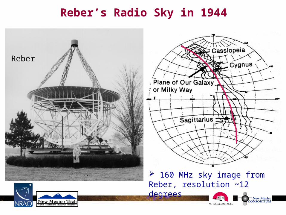
Reber’s Radio Sky in 1944

160 MHz sky image from Reber, resolution ~12 degrees

Reber

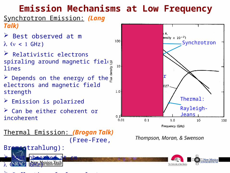
Emission Mechanisms at Low FrequencySynchrotron Emission: (Lang Talk)

Best observed at m λνGHz)

Relativistic electrons spiraling around magnetic field lines

Depends on the energy of the electrons and magnetic field strength

Emission is polarized

Can be either coherent or incoherent

Thermal Emission: (Brogan Talk) (Free-Free, Bremsstrahlung): Best observed at cm λνGHz)

Deflection of free electrons by ions

Depends on temperature of the gas

Can be emission or absorption at low νThompson, Moran, & Swenson

Synchrotron self absorption or free-free absorption

Thermal:

Rayleigh-Jeans

Synchrotron

Recombination Lines

Radio Recombination Lines: (Lang Talk) High quantum number n state (n>100 for low frequencies), formed in transition region between fully ionized regions and neutral gas (PDRs)

Nomenclature: n+Δn→n, Δn=1 is nα, Δn=2 is nβ, νo∝Δn/n3 (e.g. C441α)

Largely observed toward the Galactic Plane and discrete source. Detected in absorption below ~150 MHz.

Diagnostics of the physical conditions of the poorly probed cold ISM, e.g. temperature, density, level of ionization, abundance ratios

Frequency variable signal could adversely impact sensitive Dark Ages and Epoch of Reionization observations.

Stepkin et al. (2007)

Spatial resolution depends on wavelength and antenna diameter: First long wavelength antennas had very low spatial resolution Astronomers pushed for higher resolution and moved to higher frequencies were the TSYS is also lower:

Fundamental Limitation

θ ~ 1’, rms ~ 3 mJy/beamθ ~ 10’, rms ~ 30 mJy/beam

Confusion:(McKinnon Talk)

Low frequency instruments had limited aperture due to ionosphere (B< 5 km)

Why ‘Abandon’ Low Frequencies?

Confusion limit reached quickly with only short baselines Imaging large fields of view posed enormous computing problem Removal of radio frequency interference (RFI) was very difficult

Currently in a transition of moving to high resolution at low frequencies

Why has this taken nearly 50 years?

Software/Computing:

- Ionospheric decorrelation on baselines > 5 km is overcome by software advances of Self-Calibration in the 1980’s

- Wide-field imaging only recently (sort of) possible

- RFI excision development

- Data transmission from long distances became feasible using fiber-optic transmission lines

Overcoming the Resolution Problem

Instrument Location ν range Resolution FoV Sensitivity

(MHz) (arcsec) (arcmin) (mJy)VLA NM 73.8, 330 24-5 700-150 20-0.2GMRT IN 151-610 20-5 186-43 1.5-0.02WSRT NL 115-615 160-30 480-84

5.0-0.15…LOFAR-Low NL 10-90 40-8 1089-220 110-12LOFAR-Hi NL 110-250 5-3 272-136 0.41-0.46LWA NM 10-88 16-1.8 16-1.6

1.0 …..

Low Frequency ArraysDishes

Dipoles

Recent advances in ionospheric calibration, widefield imaging, and RFI excision have led to a new focus on low frequency arrays

★

★ 330 MHz system not compatible with EVLA, 74 MHz system to be evaluated soon – New receiver system under development

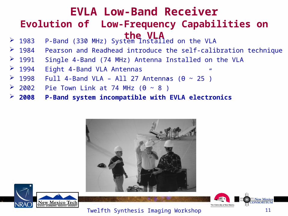
EVLA Low-Band ReceiverEvolution of Low-Frequency Capabilities on

the VLA 1983 P-Band (330 MHz) System Installed on the VLA 1984 Pearson and Readhead introduce the self-calibration technique 1991 Single 4-Band (74 MHz) Antenna Installed on the VLA 1994 Eight 4-Band VLA Antennas 1998 Full 4-Band VLA – All 27 Antennas (Ɵ ~ 25”) 2002 Pie Town Link at 74 MHz (Ɵ ~ 8”) 2008 P-Band system incompatible with EVLA electronics

11Twelfth Synthesis Imaging Workshop

EVLA Low-Band ReceiverDesign Goals for New Low-Frequency Receiver

Restore legacy low-frequency (LF) capabilities to EVLA Improve sensitivity with lower receiver noise temperature

Marian Pospiezalski of NRAO CDL building P band amplifier 4 band and spare channel amplifiers are commercial devices

Increase receiver bandwidth to enable future broadband feeds Consolidation of LF capabilities into a single receiver subsystem Provide an easily extensible platform for future LF feeds

• Two completely independent “spare” channels provideLNA –Ultra-Low Noise front end with high-dynamic rangeNoise CalibrationFilter position to define a future frequency band

Upgrades to EVLA IF structure could enable frequency coverage from 50 MHz to 1 GHz

12Twelfth Synthesis Imaging Workshop

EVLA Low-Band ReceiverIncreased Bandwidth

4-band: Increased from 1.5 MHz to ~16 MHz (66 to 82 MHz)Limited on low end by present EVLA IF structureLimited on high end by start of FM band (87.5 MHz)

P-band: Bandwidth increased from 40 MHz to 240 MHz (230 to 470 MHz)

13Twelfth Synthesis Imaging Workshop

EVLA Low-Band ReceiverConsolidated LF Platform to Enable Feed

Development

15Twelfth Synthesis Imaging Workshop

P-Band230 – 470 MHz

P-Band230 – 470 MHz

4-Band66 – 82 MHz

4-Band66 – 82 MHz

Spare BTBD

Exclusive of P-Band and 4-Band Coverage

Spare BTBD

Exclusive of P-Band and 4-Band Coverage

Spare ATBD

Exclusive of P-Band and 4-Band Coverage

Spare ATBD

Exclusive of P-Band and 4-Band Coverage

XLP

YLP

XLP

YLP

XLP

YLP

XLP

YLP

Power SupplyTemperature Monitoring

Noise Calibration InjectionCombine Channels

Power SupplyTemperature Monitoring

Noise Calibration InjectionCombine Channels

XLP

YLP

Low Frequency Science➢ Key science drivers at low frequencies: - Dark Ages (spin decoupling) - Epoch of Reionization (highly redshifted 21 cm lines) - Early Structure Formation (high z RG) - Large Scale Structure evolution (diffuse emission) - Evolution of Dark Matter & Dark Energy (Clusters) - Wide Field (up to all-sky) mapping

- Large Surveys - Transient Searches (including extrasolar planets)

- Galaxy Evolution (distant starburst galaxies) - Interstellar Medium (CR, HII regions, SNR, pulsars) - Solar Burst Studies - Ionospheric Studies - Ultra High Energy Cosmic Ray Airshowers - Serendipity (exploration of the unknown)

Dark Ages

EoR Spin temperature decouples from CMB at z~200 (νMHz) and remains below until z~30 (νMHz) Neutral hydrogen absorbs CMB and imprints inhomogeneities

Dark Ages

Loeb (2006)

Dark Ages

EoR

EoR Intruments: MWA, LOFAR, 21CMA, PAPER, SKA

Hydrogen 21 cm line during EoR between z~6 (ν ~ 200 MHz) and z~11 (ν ~ 115 MHz)

Epoch of Reionization

Tozzi et al. (2000)

Structure Formation

Dark Ages

EoR

Structure Formation

Clarke & Ensslin (2006) Galaxy clusters form through mergers and are identified by large regions of diffuse synchrotron emission (halos and relics) Important for study of plasma microphysics, dark matter and dark energy

4835 MHz 8465 MHz

1400 MHz

330 MHz

?

X-ray residuals

Clarke et al. (2005)

Evolution of AGN Activity/Feedback

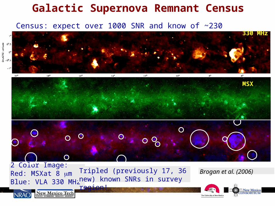
2 Color Image:Red: MSXat 8 μmBlue: VLA 330 MHz

Tripled (previously 17, 36 new) known SNRs in survey region!

Brogan et al. (2006)

Galactic Supernova Remnant Census

➢ Census: expect over 1000 SNR and know of ~230330 MHz

8 μmMSX

Hyman, et al., (2005) - Nature; Hyman et al. (2006, 2007)

GCRT J1745-3009~10 minute bursts every 77 minutes – timescale implies coherent emission

Coherent GC bursting source

Transients: Galactic Center

➢ Filaments trace magnetic field lines and particle distribution➢ Transients: sensitive, wide fields at low frequencies provide powerful opportunity to search for new transient sources➢ Candidate coherent emission transient discovered near Galactic center

Lang et al. (1999)

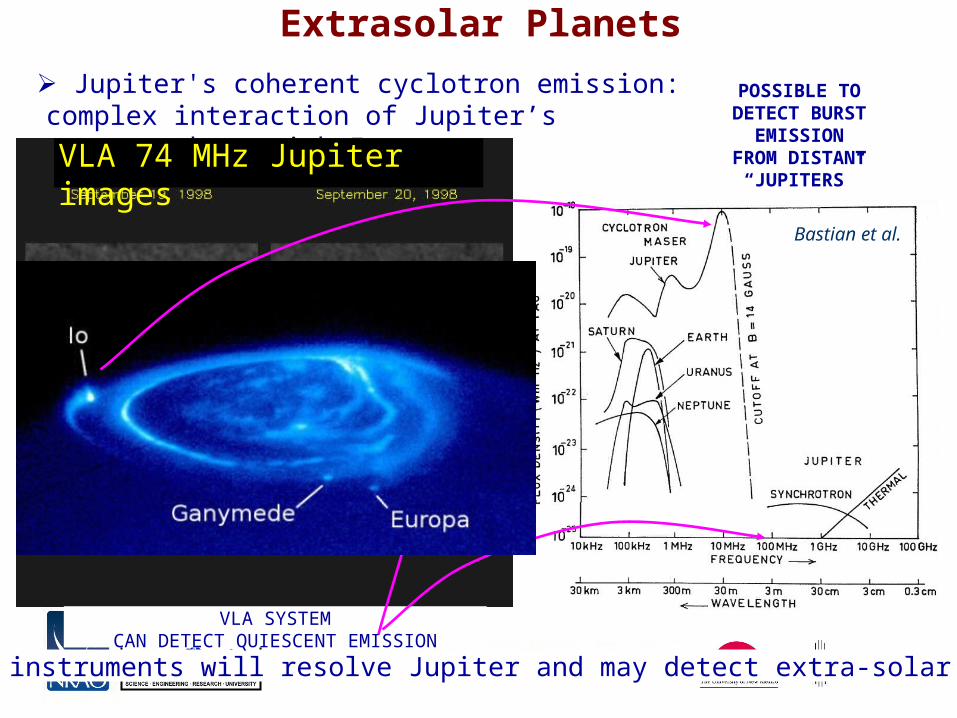
POSSIBLE TO DETECT BURST

EMISSIONFROM DISTANT

“JUPITERS”

Future instruments will resolve Jupiter and may detect extra-solar planets

➢ Jupiter's coherent cyclotron emission: complex interaction of Jupiter’s magnetosphere with Io torus

VLA 74 MHz Jupiter images

Bastian et al.

Extrasolar Planets

VLA SYSTEMCAN DETECT QUIESCENT EMISSION

VLA Low Frequency Sky Survey: VLSS

Survey Parameters: ν = 74 MHz, δ> -30°,Θ 80” resolution, σ~100 mJy/beam

Deepest & largest LF survey N ~ 70 000 sources in ~ 95% of sky > -30° Statistically useful samples of rare sources => fast pulsars, distant radio galaxies, cluster radio halos and relics, unbiased view of parent populations for unification models

Important calibration grid for EVLA, GMRT, & future LF instruments Data online at NED & http://lwa.nrl.navy.mil/VLSS

Cohen et al. 2007, AJ, 134, 1245

Cohen et al. (2007)

19

~20o

VLSS FIELD 1700+690θ~80”, rms ~50 mJy

Low Frequency In Practice: Not Easy!

Bandwidth smearing:

Distortion of sources with distance from phase center

Finite Isoplanatic Patch Problem:

Calibration changes as a function of position

Radio Frequency Interference:

Severe at low frequencies Large Fields of View:

Non-coplanar array (u,v, & w)

Large number of sources requiring deconvolution

Calibrators

Phase coherence through ionosphere

Corruption of coherence of phase on longer baselines

Not Easy but certainly possible!

Lane et al. (2001)

VLA + Pie Town outrigger (73 km)Delaney (2004)

74/330 MHz Spectral Index

Ionospheric Effects

Wedge Effects: Faraday rotation, refraction, absorption below ~ 5 MHz (atmospheric cutoff)Wave and Turbulence Effects: Rapid phase winding, differential refraction, source distortion, scintillations

~ 1000 km

~ 50 km

WedgeWaves

Wedge: characterized by TEC = ∫nedl ~ 1017 m-2

Extra path length adds extra phase ΔL α λ2 ∗ TEC Δφ ~ ΔL λ⁄ ~ λ * TEC

Waves: tiny (<1%) fluctuations superimposed on the wedge

The wedge introduces thousands of turns of phase at 74 MHz

Interferometers are particularly sensitive to difference in phase (wave/turbulence component)

~ 50 km

> 5 km<5 km

Ionosphere

Waves in the ionosphere introduce rapid phase variations (~1°/s on 35 km BL) Phase coherence is preserved on BL < 5km (gradient)

BL > 5 km have limited coherence times Without proper algorithms this limits the capabilities of low frequency instruments

Correlation preserved Correlation destroyed

F-layer 400 km

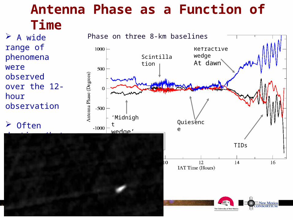
Antenna Phase as a Function of Time

A wide range of phenomena were observed over the 12-hour observation

Often daytime (but not dawn) has very good conditions

Scintillation

Refractive wedgeAt dawn

Quiesence‘Midnightwedge’

TIDs

Phase on three 8-km baselines

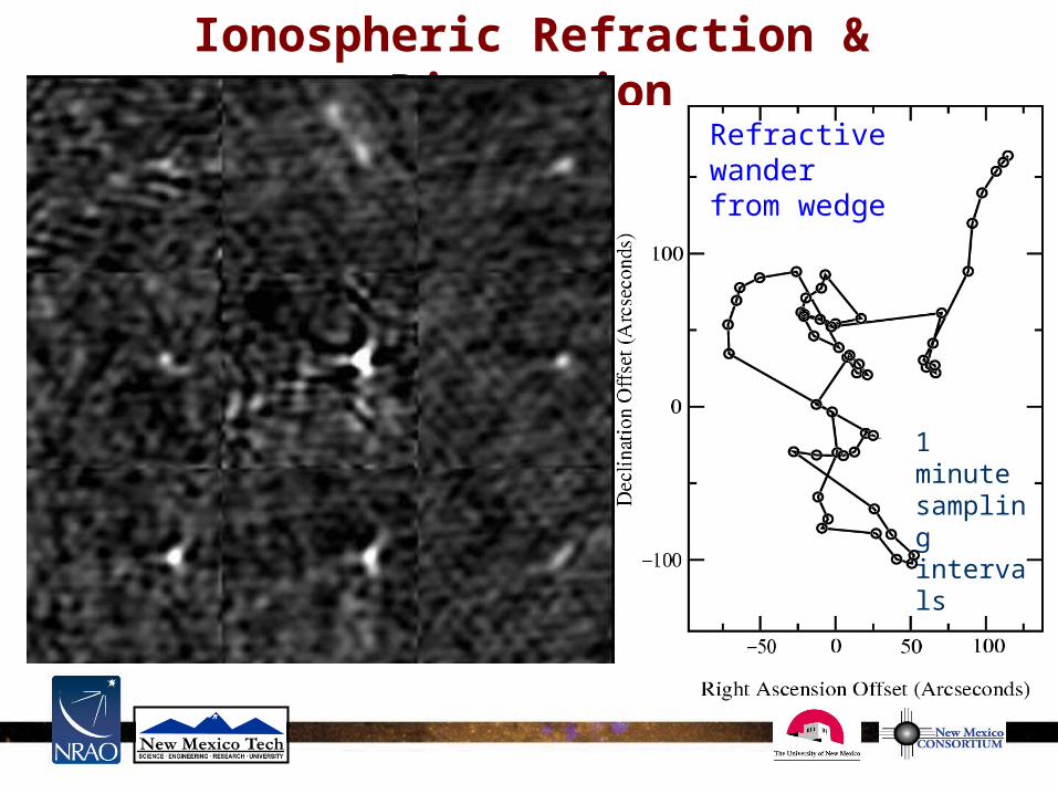
Ionospheric Refraction & Distortion

• Both global and differential refraction seen.

• Time scales of 1 min. or less.

• Equivalent length scales in the ionosphere of 10 km or less.

1 minute samplingintervals

Refractive wanderfrom wedge

Ionospheric Differential Refraction

Cohen et al (2009)

Field-Based Calibration

Average positional error decreased from ~45” to 17”

Obit: IonImage [for Obit see B. Cotton (NRAO) webpage]

Self-Calibration

Field-Based Calibration

Time-variable ZernikePolynomial Phase Screens

Rapid images of bright sources to compare to known positions Fit Zernike polynomial phase delay screen for each time interval. Apply time variable phase delay screen to produce corrected image.

Other methods are under development

Bandwidth Smearing

Averaging visibilities over finite BW results in chromatic aberration worsens with distance from the phase center => radial smearing

Δννο)x(θοθsynth ~ 2 => Io/I = 0.5 => worse at higher resolutions

Solution: spectral line mode (already essential for RFI excision)

Rule of thumb for full primary beam targeted imaging in A config. with less than 10% degradation:

74 MHz channel width < 0.06 MHz 330 MHz channel width < 0.3 MHz 1420 MHz channel width < 1.5 MHz

(Perley Lecture I)

Natural & man-generated RFI are a nuisance Getting “better” at low freq., relative BW for commercial use is low

At VLA: many different signatures seen at 74 and 330 MHz signatures: narrowband, wideband, time varying, ‘wandering’ Solar effects – unpredictable Quiet sun is a benign 2000 Jy disk at 74 MHz Solar bursts, geomagnetic storms are disruptive => 109 Jy! Powerful Solar bursts can occur even at Solar minimum! Can be wideband (C & D configurations), mostly narrowband

Best to deal with RFI at highest spectral resolution before averaging for imaging.

Radio Frequency Interference: RFI

Tim

e

RFI environment worse on short baselines

Several 'types': narrow band, wandering, wideband, ...

Wideband interference hard for some automated routines

Example using AIPS tasksFLGIT, FLAGR, RFI, NEW: UVRFI

RFI Examples

(Pen Talk)

Short baseline Long baseline

RFI Excision vs Cancellation

Time

Frequency

Many algorithms handle RFI through excision

• OK if you have little RFI or lots of data

Ideally we want to remove RFI and leave the data

Current development aimed at cancellation Fringe stopping works well for constant RFI but not moving or time variable

Full removal will likely require algorithms using multiple techniques

Time

Frequency

Helmboldt et al. (in prep.)

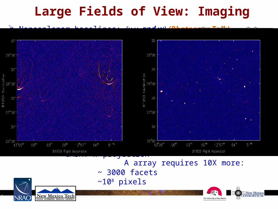
Large Fields of View: Imaging Noncoplanar baselines: (u,v, and w) (Bhatnagar Talk)

Important if , shape of array varies over FoV

=> in AIPS multi-facet imaging,

=> in CASA w-projection or facets

Essential for all observations below 1 GHz and for high resolution, high dynamic range even at 1.4 GHz, reduces sidelobes of confusing sources

Requires lots of computing power and disk space

AIPS: IMAGR (DO3DIMAG=1, NFIELD=N, OVERLAP=2) CASA: w-projection

Example: VLA B array 74 MHz:~325 facets

A array requires 10X more:~ 3000 facets~108 pixels

Full Field vs Targeted Imaging

2D faceted imaging of entire FoV is very computationally expensive

2D “tile”

74 MHz Wide-field VLA Image

~10 degree VLSS Image

Fly’s Eye

OutliersA

arr

ay r

equ

ires

~10

,000

pix

els!

Fly’s eye of field center and then targeted facets on outlier is less demanding BUT potential loss of interesting science

Large Fields of View: Calibration

Antenna gain (phase and amplitude) and to a lesser degree bandpass calibration depends on assumption that calibrator is a single POINT source

• Large FOV + low freq. = numerous sources everywhere

At 330 MHz, calibrator should dominate flux in FOV: extent to which this is true affects absolute positions and flux scale

=> Phases (but not positions) can be improved by self-calibrating phase calibrator

=> Always check accuracy of positions

Must use source with accurate model for bandpass and instrumental phase CygA, CasA, TauA, VirgoA

330 MHz phase calibrator: 1833-210

9 Jy

1 Jy

Summary Recent progress in wide-field imaging, RFI excision/cancellation, and ionospheric calibration are opening the low frequency spectrum to arcsecond resolution and mJy sensitivities – stay tuned for latest developments

Advances will lead improved scientific capabilities for studies from Dark Ages to the ionosphere

Next generation of low frequency instruments is being built while current instruments (such as the EVLA) are being upgraded

NRAO plans testing of the 4 band system in the upcoming C configuration and hopes to re-deploy it in B/BnA/A configs

Development of new P band system anticipates having new receivers ready by Nov. 2011

Initially observations will likely continue to use the old feeds but ideally new broadband feeds will be developed