December 3, 2003 12:13 00851

Tutorials and Reviews

International Journal of Bifurcation and Chaos, Vol. 13, No. 11 (2003) 3147–3233c© World Scientific Publishing Company

TOWARD A THEORY OF CHAOS

A. SENGUPTADepartment of Mechanical Engineering,Indian Institute of Technology Kanpur,

Kanpur 208016, Indiaosegu@iitk.ac.in

Received February 23, 2001; Revised September 19, 2002

This paper formulates a new approach to the study of chaos in discrete dynamical systemsbased on the notions of inverse ill-posed problems, set-valued mappings, generalized and multi-valued inverses, graphical convergence of a net of functions in an extended multifunction space[Sengupta & Ray, 2000], and the topological theory of convergence. Order, chaos and complexityare described as distinct components of this unified mathematical structure that can be viewedas an application of the theory of convergence in topological spaces to increasingly nonlinearmappings, with the boundary between order and complexity in the topology of graphical con-vergence being the region in (Multi(X)) that is susceptible to chaos. The paper uses results fromthe discretized spectral approximation in neutron transport theory [Sengupta, 1988, 1995] andconcludes that the numerically exact results obtained by this approximation of the Case singulareigenfunction solution is due to the graphical convergence of the Poisson and conjugate Poissonkernels to the Dirac delta and the principal value multifunctions respectively. In (Multi(X)),the continuous spectrum is shown to reduce to a point spectrum, and we introduce a notion oflatent chaotic states to interpret superposition over generalized eigenfunctions. Along with theselatent states, spectral theory of nonlinear operators is used to conclude that nature supportscomplexity to attain efficiently a multiplicity of states that otherwise would remain unavailableto it.

Keywords : Chaos; complexity; ill-posed problems; graphical convergence; topology; multifunc-tions.

Prologue

1. Generally speaking, the analysis of chaos is ex-

tremely difficult. While a general definition for chaos

applicable to most cases of interest is still lacking,mathematicians agree that for the special case of iter-

ation of transformations there are three common char-

acteristics of chaos:

1. Sensitive dependence on initial conditions,2. Mixing,3. Dense periodic points.

[Peitgen, Jurgens & Saupe, 1992]

2. The study of chaos is a part of a larger program

of study of so-called “strongly” nonlinear system.

. . . Linearity means that the rule that determines what

a piece of a system is going to do next is not influ-

enced by what it is doing now. More precisely this

is intended in a differential or incremental sense: For

a linear spring, the increase of its tension is propor-

tional to the increment whereby it is stretched, with

the ratio of these increments exactly independent of

how much it has already been stretched. Such a spring

can be stretched arbitrarily far . . . . Accordingly no real

spring is linear. The mathematics of linear objects is

particularly felicitous. As it happens, linear objects en-

joy an identical, simple geometry. The simplicity of

3147

December 3, 2003 12:13 00851

3148 A. Sengupta

this geometry always allows a relatively easy mental

image to capture the essence of a problem, with the

technicality, growing with the number of parts, basi-

cally a detail. The historical prejudice against nonlinear

problems is that no so simple nor universal geometry

usually exists.

Mitchell Feigenbaum’s Foreword (pp. 1–7)in [Peitgen et al., 1992]

3. The objective of this symposium is to explore the

impact of the emerging science of chaos on various dis-

ciplines and the broader implications for science and

society. The characteristic of chaos is its universality

and ubiquity. At this meeting, for example, we have

scholars representing mathematics, physics, biology,geophysics and geophysiology, astronomy, medicine,psychology, meteorology, engineering, computer sci-

ence, economics and social sciences.1 Having so many

disciplines meeting together, of course, involves the

risk that we might not always speak the same lan-

guage, even if all of us have come to talk about

“chaos”.

Opening address of Heitor Gurgulino de Souza,Rector United Nations University, Tokyo

[de Souza, 1997]

4. The predominant approach (of how the different

fields of science relate to one other) is reductionist:Questions in physical chemistry can be understood

in terms of atomic physics, cell biology in terms of

how biomolecules work . . . . We have the best of rea-

sons for taking this reductionist approach: it works.

But shortfalls in reductionism are increasingly appar-

ent (and) there is something to be gained from sup-

plementing the predominantly reductionist approach

with an integrative agenda. This special section on

complex systems is an initial scan (where) we have

taken a “complex system” to be one whose properties

are not fully explained by an understanding of its com-

ponent parts. Each Viewpoint author 2 was invited to

define “complex” as it applied to his or her discipline.

[Gallagher & Appenzeller, 1999]

5. One of the most striking aspects of physics

is the simplicity of its laws. Maxwell’s equations,Schroedinger’s equations, and Hamilton mechanics

can each be expressed in a few lines. . . . Everything

is simple and neat except, of course, the world. Every

place we look outside the physics classroom we see a

world of amazing complexity. . . . So why, if the laws

are so simple, is the world so complicated? To us com-

plexity means that we have structure with variations.

Thus a living organism is complicated because it has

many different working parts, each formed by varia-

tions in the working out of the same genetic coding.

Chaos is also found very frequently. In a chaotic world

it is hard to predict which variation will arise in a given

place and time. A complex world is interesting because

it is highly structured. A chaotic world is interesting

because we do not know what is coming next. Our

world is both complex and chaotic. Nature can pro-

duce complex structures even in simple situations and

obey simple laws even in complex situations.

[Goldenfeld & Kadanoff, 1999]

6. Where chaos begins, classical science stops. For as

long as the world has had physicists inquiring into

the laws of nature, it has suffered a special ignorance

about disorder in the atmosphere, in the turbulent sea,in the fluctuations in the wildlife populations, in the

oscillations of the heart and the brain. But in the 1970s

a few scientists began to find a way through disor-

der. They were mathematicians, physicists, biologists,chemists . . . (and) the insights that emerged led di-

rectly into the natural world : the shapes of clouds,the paths of lightning, the microscopic intertwining

of blood vessels, the galactic clustering of stars. . . .Chaos breaks across the lines that separate scientific

disciplines, (and) has become a shorthand name for a

fast growing movement that is reshaping the fabric of

the scientific establishment.

[Gleick, 1987]

7. order (→) complexity (→) chaos.

[Waldrop, 1992]

1A partial listing of papers is as follows: Chaos and Politics: Application of Nonlinear Dynamics to Socio-Political issues;Chaos in Society: Reflections on the Impact of Chaos Theory on Sociology; Chaos in Neural Networks; The Impact of Chaos

on Mathematics; The Impact of Chaos on Physics; The Impact of Chaos on Economic Theory; The Impact of Chaos on

Engineering; The impact of Chaos on Biology; Dynamical Disease: And The Impact of Nonlinear Dynamics and Chaos on

Cardiology and Medicine.2The eight Viewpoint articles are titled: Simple Lessons from Complexity; Complexity in Chemistry; Complexity in Biolog-

ical Signaling Systems; Complexity and the Nervous System; Complexity, Pattern, and Evolutionary Trade-Offs in Animal

Aggregation; Complexity in Natural Landform Patterns; Complexity and Climate, and Complexity and the Economy.

December 3, 2003 12:13 00851

Toward a Theory of Chaos 3149

8. Our conclusions based on these examples seem sim-

ple: At present chaos is a philosophical term, not a

rigorous mathematical term. It may be a subjective

notion illustrating the present day limitations of the

human intellect or it may describe an intrinsic prop-

erty of nature such as the “randomness” of the se-

quence of prime numbers. Moreover, chaos may be

undecidable in the sense of Godel in that no matter

what definition is given for chaos, there is some ex-

ample of chaos which cannot be proven to be chaotic

from the definition.

[Brown & Chua, 1996]

9. My personal feeling is that the definition of a “frac-tal” should be regarded in the same way as the biolo-

gist regards the definition of “life”. There is no hard

and fast definition, but just a list of properties char-

acteristic of a living thing . . . . Most living things have

most of the characteristics on the list, though there

are living objects that are exceptions to each of them.

In the same way, it seems best to regard a fractal as

a set that has properties such as those listed below,rather than to look for a precise definition which will

certainly exclude some interesting cases.

[Falconer, 1990]

10. Dynamical systems are often said to exhibit chaos

without a precise definition of what this means.

[Robinson, 1999]

1. Introduction

The purpose of this paper is to present an unified,self-contained mathematical structure and physicalunderstanding of the nature of chaos in a discretedynamical system and to suggest a plausible expla-nation of why natural systems tend to be chaotic.The somewhat extensive quotations with which webegin above, bear testimony to both the increas-ingly significant — and perhaps all-pervasive —role of nonlinearity in the world today as also ourimperfect state of understanding of its manifesta-tions. The list of papers at both the UN Confer-ence [de Souza, 1997] and in Science [Gallagher &Appenzeller, 1999] is noteworthy if only to justifythe observation of Gleick [1987] that “chaos seemsto be everywhere”. Even as everybody appears tobe finding chaos and complexity in all likely andunlikely places, and possibly because of it, it is nec-

essary that we have a mathematically clear physi-cal understanding of these notions that are suppos-edly reshaping our view of nature. This paper is anattempt to contribute to this goal. To make thisaccount essentially self-contained we include here,as far as this is practical, the basics of the back-ground material needed to understand the paper inthe form of Tutorials and an extended Appendix.

The paradigm of chaos of the kneading of thedough is considered to provide an intuitive basisof the mathematics of chaos [Peitgen et al., 1992],and one of our fundamental objectives here is to re-count the mathematical framework of this processin terms of the theory of ill-posed problems arisingfrom non-injectivity [Sengupta, 1997], maximal ill-posedness, and graphical convergence of functions[Sengupta & Ray, 2000]. A natural mathematicalformulation of the kneading of the dough in theform of stretch-cut-and-paste and stretch-cut-and-fold operations is in the ill-posed problem arisingfrom the increasing non-injectivity of the functionf modeling the kneading operation.

Begin Tutorial 1: Functions andMultifunctions

A relation, or correspondence, between two sets X

and Y , written M: X–→→Y , is basically a rule that

associates subsets of X to subsets of Y ; this is oftenexpressed as (A, B) ∈ M where A ⊂ X and B ⊂ Yand (A, B) is an ordered pair of sets. The domain

D(M)def= A ⊂ X : (∃Z ∈ M)(πX(Z) = A)

and range

R(M)def= B ⊂ Y : (∃Z ∈ M)(πY (Z) = B)

of M are respectively the sets of X which underM corresponds to sets in Y ; here πX and (πY )are the projections of Z on X and Y , respectively.Equivalently, (D(M) = x ∈ X : M(x) 6= ∅) and(R(M) =

⋃

x∈D(M) M(x)). The inverse M− of Mis the relation

M− = (B, A) : (A, B) ∈ Mso that M− assigns A to B iff M assigns B to A.In general, a relation may assign many elements inits range to a single element from its domain; of

December 3, 2003 12:13 00851

3150 A. Sengupta

(d)

(b)(a)

(c)

(a)

(d)

(b)(a)

(c)

(b)

(d)

(b)(a)

(c)

! "

(c) (d)

(b)(a)

(c)

#$

% &' (

(d)

Fig. 1. Functional and non-functional relations between two sets X and Y : while f and g are functional relations, M is not.(a) f and g are both injective and surjective (i.e. they are bijective), (b) g is bijective but f is only injective and f−1(y2) := ∅,(c) f is not 1:1, g is not onto, while (d) M is not a function but is a multifunction.

especial significance are functional relations f 3 thatcan assign only a unique element in R(f) to anyelement in D(f). Figure 1 illustrates the distinc-tion between arbitrary and functional relations Mand f . This difference between functions (or maps)and multifunctions is basic to our development andshould be fully understood. Functions can again beclassified as injections (or 1:1) and surjections (oronto). f : X → Y is said to be injective (or one-to-one) if x1 6= x2 ⇒ f(x1) 6= f(x2) for all x1, x2 ∈ X,while it is surjective (or onto) if Y = f(X). f isbijective if it is both 1:1 and onto.

Associated with a function f : X → Y is its in-verse f−1: Y ⊇ R(f) → X that exists on R(f) ifff is injective. Thus when f is bijective, f−1(y) :=x ∈ X: y = f(x) exists for every y ∈ Y ; infact f isbijective iff f−1(y) is a singleton for each y ∈ Y .Non-injective functions are not at all rare; if any-thing, they are very common even for linear mapsand it would be perhaps safe to conjecture thatthey are overwhelmingly predominant in the non-linear world of nature. Thus for example, the simple

linear homogeneous differential equation with con-stant coefficients of order n > 1 has n linearlyindependent solutions so that the operator Dn ofDn(y) = 0 has a n-dimensional null space. Inversesof non-injective, and in general non-bijective, func-tions will be denoted by f−. If f is not injectivethen

A ⊂ f−f(A)def= sat(A)

where sat(A) is the saturation of A ⊆ X induced byf ; if f is not surjective then

ff−(B) := B⋂

f(X) ⊆ B.

If A = sat(A), then A is said to be saturated, andB ⊆ R(f) whenever ff−(B) = B. Thus for non-injective f , f−f is not an identity on X just asff− is not 1Y if f is not surjective. However theset of relations

ff−f = f, f−ff− = f− (1)

that is always true will be of basic significance inthis work. Following are some equivalent statements

3We do not distinguish between a relation and its graph although technically they are different objects. Thus although afunctional relation, strictly speaking, is the triple (X, f, Y ) written traditionally as f : X → Y , we use it synonymously withthe graph f itself. Parenthetically, the word functional in this paper is not necessarily employed for a scalar-valued function,but is used in a wider sense to distinguish between a function and an arbitrary relation (that is a multifunction). Formally,whereas an arbitrary relation from X to Y is a subset of X × Y , a functional relation must satisfy an additional restrictionthat requires y1 = y2 whenever (x, y1) ∈ f and (x, y2) ∈ f . In this subset notation, (x, y) ∈ f ⇔ y = f(x).

December 3, 2003 12:13 00851

Toward a Theory of Chaos 3151

on the injectivity and surjectivity of functions f :X → Y .

(Injec) f is 1:1 ⇔ there is a function fL: Y → Xcalled the left inverse of f , such that fLf = 1X ⇔A = f−f(A) for all subsets A of X ⇔ f(

⋂

Ai) =⋂

f(Ai).

(Surjec) f is onto ⇔ there is a function fR: Y → Xcalled the right inverse of f , such that ffR = 1Y ⇔B = ff−(B) for all subsets B of Y .

As we are primarily concerned with non-injectivity of functions, saturated sets generated byequivalence classes of f will play a significant rolein our discussions. A relation E on a set X is saidto be an equivalence relation if it is4

(ER1) Reflexive: (∀x ∈ X)(xEx).(ER2) Symmetric: (∀x, y ∈ X)(xEy ⇒ yEx).(ER3) Transitive: (∀x, y, z ∈ X)(xEy ∧ yEz ⇒

xEz).Equivalence relations group together unequal ele-ments x1 6= x2 of a set as equivalent according tothe requirements of the relation. This is expressedas x1 ∼ x2(mod E) and will be represented here bythe shorthand notation x1 ∼E x2, or even simplyas x1 ∼ x2 if the specification of E is not essential.Thus for a non-injective map if f(x1) = f(x2) forx1 6= x2, then x1 and x2 can be considered to beequivalent to each other since they map onto thesame point under f ; thus x1 ∼f x2 ⇔ f(x1) =f(x2) defines the equivalence relation ∼f inducedby the map f . Given an equivalence relation ∼ ona set X and an element x ∈ X the subset

[x]def= y ∈ X : y ∼ x

is called the equivalence class of x; thus x ∼ y ⇔[x] = [y]. In particular, equivalence classes gener-ated by f : X → Y , [x]f = xα ∈ X : f(xα) =f(x), will be a cornerstone of our analysis of chaosgenerated by the iterates of non-injective maps, andthe equivalence relation ∼f := (x, y): f(x) = f(y)generated by f is uniquely defined by the partitionthat f induces on X. Of course as x ∼ x, x ∈ [x].It is a simple matter to see that any two equiva-lence classes are either disjoint or equal so that theequivalence classes generated by an equivalence re-lation on X form a disjoint cover of X. The quotient

set of X under ∼, denoted by X/∼:= [x]: x ∈ X,has the equivalence classes [x] as its elements; thus[x] plays a dual role either as subsets of X or as ele-ments of X/∼. The rule x 7→ [x] defines a surjectivefunction Q: X → X/∼ known as the quotient map.

Example 1.1. Let

S1 = (x, y) ∈ R2) : x2 + y2 = 1

be the unit circle in R2. Consider X = [0, 1] as asubspace of R, define a map

q : X → S1, s 7→ (cos 2πs, sin 2πs), s ∈ X ,

from R to R2, and let ∼ be the equivalence relationon X

s ∼ t⇔ (s = t) ∨ (s = 0, t = 1) ∨ (s = 1, t = 0) .

If we bendX around till its ends touch, the resultingcircle represents the quotient set Y = X/∼ whosepoints are equivalent under ∼ as follows

[0] = 0, 1 = [1], [s] = s for all s ∈ (0, 1) .

Thus q is bijective for s ∈ (0, 1) but two-to-one forthe special values s = 0 and 1, so that for s, t ∈ X,

s ∼ t⇔ q(s) = q(t) .

This yields a bijection h: X/∼→ S1 such that

q = h Qdefines the quotient map Q: X → X/∼ by h([s]) =q(s) for all s ∈ [0, 1]. The situation is illustrated bythe commutative diagram of Fig. 2 that appears asan integral component in a different and more gen-eral context in Sec. 2. It is to be noted that com-mutativity of the diagram implies that if a givenequivalence relation ∼ on X is completely deter-mined by q that associates the partitioning equiva-lence classes in X to unique points in S1, then ∼ isidentical to the equivalence relation that is inducedby Q onX. Note that a larger size of the equivalenceclasses can be obtained by considering X = R+ forwhich s ∼ t⇔ |s− t| ∈ Z+.

End Tutorial 1

4An alternate useful way of expressing these properties for a relation R on X are(ER1) R is reflexive iff 1X ⊆ X(ER2) R is symmetric iff R = R−1

(ER3) R is transitive iff R R ⊆ R,with R an equivalence relation only if R R = R.

December 3, 2003 12:13 00851

3152 A. Sengupta

Fig. 2. The quotient map Q.

One of the central concepts that we consider andemploy in this work is the inverse f− of a nonlin-ear, non-injective, function f ; here the equivalenceclasses [x]f = f−f(x) of x ∈ X are the saturatedsubsets of X that partition X. While a detailedtreatment of this question in the form of the non-linear ill-posed problem and its solution is given inSec. 2 [Sengupta, 1997], it is sufficient to point outhere from Figs. 1(c) and 1(d), that the inverse of anon-injective function is not a function but a mul-tifunction while the inverse of a multifunction is anon-injective function. Hence one has the generalresult that

f is a non-injective function⇔ f− is a multifunction .

f is a multifunction⇔ f− is a non-injective function

(2)

The inverse of a multifunction M: X–→→Y is a gen-

eralization of the corresponding notion for a func-tion f : X → Y such that

M−(y)def= x ∈ X : y ∈ M(x)

leads to

M−(B) = x ∈ X : M(x)⋂

B 6= ∅

for any B ⊆ Y , while a more restricted inversethat we shall not be concerned with is given asM+(B) = x ∈ X : M(x) ⊆ B. Obviously,M+(B) ⊆ M−(B). A multifunction is injective ifx1 6= x2 ⇒ M(x1)

⋂M(x2) = ∅, and commonlywith functions, it is true that M

(⋃

α∈DAα

)

=

⋃

α∈D M(Aα) and M(⋂

α∈D Aα

)

⊆ ⋂

α∈D M(Aα)where D is an index set. The following illustratesthe difference between the two inverses of M. LetX be a set that is partitioned into two disjoint M-invariant subsets X1 and X2. If x ∈ X1 (or x ∈ X2)then M(x) represents that part of X1 (or of X2)that is realized immediately after one applicationof M, while M−(x) denotes the possible precursorsof x in X1 (or of X2) and M+(B) is that subset ofX whose image lies in B for any subset B ⊂ X.

In this paper the multifunctions that we shallbe explicitly concerned with arise as the inverses ofnon-injective maps.

The second major component of our theory isthe graphical convergence of a net of functions toa multifunction. In Tutorial 2 below, we replace forthe sake of simplicity and without loss of generality,the net (which is basically a sequence where the in-dex set is not necessarily the positive integers; thusevery sequence is a net but the family5 indexed, forexample, by Z, the set of all integers, is a net andnot a sequence) with a sequence and provide thenecessary background and motivation for the con-cept of graphical convergence.

Begin Tutorial 2: Convergence ofFunctions

This Tutorial reviews the inadequacy of the usualnotions of convergence of functions either to limitfunctions or to distributions and suggests the mo-tivation and need for introduction of the notionof graphical convergence of functions to multifunc-tions. Here, we follow closely the exposition ofKorevaar [1968], and use the notation (fk)

∞k=1 to de-

note real or complex valued functions on a boundedor unbounded interval J .

A sequence of piecewise continuous functions(fk)

∞k=1 is said to converge to the function f , nota-

tion fk → f , on a bounded or unbounded intervalJ6

(1) Pointwise if

fk(x) → f(x) for all x ∈ J ,

5A function χ: D → X will be called a family in X indexed by D when reference to the domain D is of interest, and a net

when it is required to focus attention on its values in X.6Observe that it is not being claimed that f belongs to the same class as (fk). This is the single most important cornerstoneon which this paper is based: the need to “complete” spaces that are topologically “incomplete”. The classical high-schoolexample of the related problem of having to enlarge, or extend, spaces that are not big enough is the solution space of algebraicequations with real coefficients like x2 + 1 = 0.

December 3, 2003 12:13 00851

Toward a Theory of Chaos 3153

i.e. Given any arbitrary real number ε > 0 thereexists a K ∈ N that may depend on x, such that|fk(x) − f(x)| < ε for all k ≥ K.

(2) Uniformly if

supx∈J

|f(x) − fk(x)| → 0 as k → ∞ ,

i.e. Given any arbitrary real number ε > 0 thereexists a K ∈ N, such that supx∈J |fk(x)− f(x)| < εfor all k ≥ K.

(3) In the mean of order p ≥ 1 if |f(x) − fk(x)|p isintegrable over J for each k

∫

J|f(x) − fk(x)|p → 0 as k → ∞ .

For p = 1, this is the simple case of convergence inthe mean.

(4) In the mean m-integrally if it is possible to selectindefinite integrals

f(−m)k (x) = πk(x) +

∫ x

cdx1

∫ x1

cdx2

· · ·∫ xm−1

cdxmfk(xm)

and

f (−m)(x) = π(x) +

∫ x

cdx1

∫ x1

cdx2

· · ·∫ xm−1

cdxmf(xm)

such that for some arbitrary real p ≥ 1,∫

J|f (−m) − f

(−m)k |p → 0 as k → ∞.

where the polynomials πk(x) and π(x) are of degree< m, and c is a constant to be chosen appropriately.

(5) Relative to test functions ϕ if fϕ and fkϕ areintegrable over J and∫

J(fk − f)ϕ→ 0 for every ϕ ∈ C∞0 (J) as k → ∞ ,

where C∞0 (J) is the class of infinitely differentiablecontinuous functions that vanish throughout someneighborhood of each of the end points of J . Foran unbounded J , a function is said to vanish insome neighborhood of +∞ if it vanishes on someray (r, ∞).

While pointwise convergence does not implyany other type of convergence, uniform conver-gence on a bounded interval implies all the otherconvergences.

It is to be observed that apart from point-wise and uniform convergences, all the other modeslisted above represent some sort of an averaged con-tribution of the entire interval J and are thereforenot of much use when pointwise behavior of thelimit f is necessary. Thus while limits in the meanare not unique, oscillating functions are tamed bym-integral convergence for adequately large valuesof m, and convergence relative to test functions,as we see below, can be essentially reduced to m-integral convergence. On the contrary, our graphicalconvergence — which may be considered as a point-wise biconvergence with respect to both the directand inverse images of f just as usual pointwise con-vergence is with respect to its direct image only— allows a sequence (in fact, a net) of functions toconverge to an arbitrary relation, unhindered by ex-ternal influences such as the effects of integrationsand test functions. To see how this can indeed mat-ter, consider the following

Example 1.2. Let fk(x) = sinkx, k = 1, 2, . . . andlet J be any bounded interval of the real line. Then1-integrally we have

f(−1)k (x) = −1

kcos kx = −1

k+

∫ x

0sin kx1dx1 ,

which obviously converges to 0 uniformly (andtherefore in the mean) as k → ∞. And herein liesthe point: even though we cannot conclude aboutthe exact nature of sin kx as k increases indefi-nitely (except that its oscillations become more andmore pronounced), we may very definitely state thatlimk→∞(cos kx)/k = 0 uniformly. Hence from

f(−1)k (x) → 0 = 0 +

∫ x

0lim

k→∞sin kx1dx1

it follows that

limk→∞

sin kx = 0 (3)

1-integrally.Continuing with the same sequence of func-

tions, we now examine its test-functional conver-gence with respect to ϕ ∈ C1

0(−∞, ∞) that vanishesfor all x /∈ (α, β). Integrating by parts,

∫ ∞

−∞fkϕ =

∫ β

αϕ(x1) sin kx1dx1

= −1

k[ϕ(x1) cos kx1]

βα

−1

k

∫ β

αϕ′(x1) cos kx1dx1

December 3, 2003 12:13 00851

3154 A. Sengupta

(a)

(b)

! " #$

$

%&')(*(

%&')(*+

(c)

Fig. 3. Incompleteness of function spaces. (a) demonstrates the classic example of non-completeness of the space of real-valued continuous functions leading to the complete spaces Ln[a, b] whose elements are equivalence classes of functions with

f ∼ g iff the Lebesgue integral∫ b

a|f − g|n = 0. (b) and (c) illustrate distributional convergence of the functions fk(x) of

Eq. (5) to the Dirac delta δ(x) leading to the complete space of generalized functions. In comparison, note that the spaceof continuous functions in the uniform metric C[a, b] is complete which suggests the importance of topologies in determiningconvergence properties of spaces.

The first integrated term is 0 due to the condi-tions on ϕ while the second also vanishes becauseϕ ∈ C1

0(−∞, ∞). Hence

∫ ∞

−∞fkϕ→ 0 =

∫ β

αlim

k→∞ϕ(x1) sin ksdx1

for all ϕ, and leading to the conclusion that

limk→∞

sin kx = 0 (4)

test-functionally.

This example illustrates the fact that ifSupp(ϕ) = [α, β] ⊆ J ,7 integrating by parts suf-ficiently large number of times so as to wipe outthe pathological behavior of (fk) gives

∫

Jfkϕ =

∫ β

αfkϕ

=

∫ β

αf

(−1)k ϕ′ = · · · = (−1)m

∫ β

αf

(−m)k ϕm

where f(−m)k (x) = πk(x) +

∫ xc dx1

∫ x1

c dx2 · · ·∫ xm−1

cdxmfk(xm) is an m-times arbitrary indefinite in-

tegral of fk. If now it is true that∫ βα f

(−m)k →

∫ βα f (−m), then it must also be true that f

(−m)k ϕ(m)

converges in the mean to f (−m)ϕ(m) so that∫ β

αfkϕ = (−1)m

∫ β

αf

(−m)k ϕ(m)

→ (−1)m

∫ β

αf (−m)ϕ(m) =

∫ β

αfϕ.

In fact the converse also holds leading to thefollowing Equivalences between m-convergence inthe mean and convergence with respect to test-functions [Korevaar, 1968].

Type 1 Equivalence. If f and (fk) are functionson J that are integrable on every interior subinter-val, then the following are equivalent statements.

(a) For every interior subinterval I of J there isan integer mI ≥ 0, and hence a smallest in-teger m ≥ 0, such that certain indefinite inte-

grals f(−m)k of the functions fk converge in the

mean on I to an indefinite integral f (−m); thus∫

I |f(−m)k − f (−m)| → 0.

(b)∫

J(fk − f)ϕ→ 0 for every ϕ ∈ C∞0 (J).

A significant generalization of this Equivalence isobtained by dropping the restriction that the limitobject f be a function. The need for this gener-alization arises because metric function spaces are

7By definition, the support (or supporting interval) of ϕ(x) ∈ C∞0 [α, β] is [α, β] if ϕ and all its derivatives vanish for x ≤ αand x ≥ β.

December 3, 2003 12:13 00851

Toward a Theory of Chaos 3155

known not to be complete: Consider the sequenceof functions [Fig. 3(a)]

fk(x) =

0, if a ≤ x ≤ 0

kx, if 0 ≤ x ≤ 1

k

1, if1

k≤ x ≤ b

(5)

which is not Cauchy in the uniform metricρ(fj , fk) = supa≤x≤b |fj(x) − fk(x)| but is Cauchy

in the mean ρ(fj, fk) =∫ ba |fj(x) − fk(x)|dx, or

even pointwise. However in either case, (fk) cannotconverge in the respective metrics to a continuousfunction and the limit is a discontinuous unit stepfunction

Θ(x) =

0, if a ≤ x ≤ 0

1, if 0 < x ≤ b

with graph ([a, 0], 0)⋃

((0, b], 1), which is also in-tegrable on [a, b]. Thus even if the limit of the se-quence of continuous functions is not continuous,both the limit and the members of the sequenceare integrable functions. This Riemann integrationis not sufficiently general, however, and this typeof integrability needs to be replaced by a muchweaker condition resulting in the larger class ofthe Lebesgue integrable complete space of functionsL[a, b].8

The functions in Fig. 3(b),

δk(x) =

k, if 0 < x <1

k

0, x ∈ [a, b] −(

0,1

k

)

,

can be associated with the arbitrary indefiniteintegrals

Θk(x)def= δ

(−1)k (x) =

0, a ≤ x ≤ 0

kx, 0 < x <1

k

1,1

k≤ x ≤ b

of Fig. 3(c), which, as noted above, convergein the mean to the unit step function Θ(x);

hence∫∞−∞ δkϕ ≡

∫ βα δkϕ = −

∫ βα δ

(−1)k ϕ′ →

−∫ β0 ϕ′(x)dx = ϕ(0). But there can be no func-

tional relation δ(x) for which∫ βα δ(x)ϕ(x)dx = ϕ(0)

for all ϕ ∈ C10 [α, β], so that unlike in the case in

Type 1 Equivalence, the limit in the mean Θ(x)

of the indefinite integrals δ(−1)k (x) cannot be ex-

pressed as the indefinite integral δ(−1)(x) of somefunction δ(x) on any interval containing the ori-gin. This leads to the second more general type ofequivalence.

Type 2 Equivalence. If (fk) are functions on Jthat are integrable on every interior subinterval,then the following are equivalent statements.

(a) For every interior subinterval I of J there is aninteger mI ≥ 0, and hence a smallest integerm ≥ 0, such that certain indefinite integrals

f(−m)k of the functions fk converge in the mean

on I to an integrable function Θ which, unlikein Type 1 Equivalence, need not itself be anindefinite integral of some function f .

8Both Riemann and Lebesgue integrals can be formulated in terms of the so-called step functions s(x), which are piecewise

constant functions with values (σi)Ii=1on a finite number of bounded subintervals (Ji)

Ii=1 (which may reduce to a point or

may not contain one or both of the end points) of a bounded or unbounded interval J , with integral∫

Js(x)dx

def=∑I

i=1 σi|Ji|.While the Riemann integral of a bounded function f(x) on a bounded interval J is defined with respect to sequences

of step functions (sj)∞j=1 and (tj)

∞j=1 satisfying sj(x) ≤ f(x) ≤ tj(x) on J with

∫

J(sj − tj) → 0 as j → ∞ as

R∫

J f(x)dx = lim∫

J sj(x)dx = lim∫

J tj(x)dx, the less restrictive Lebesgue integral is defined for arbitrary functions f

over bounded or unbounded intervals J in terms of Cauchy sequences of step functions∫

J|si − sk| → 0, i, k → ∞, converging

to f(x) as

sj(x) → f(x) pointwise almost everywhere on J ,

to be∫

J

f(x)dxdef= lim

j→∞

∫

J

sj(x)dx .

That the Lebesgue integral is more general (and therefore is the proper candidate for completion of function spaces) isillustrated by the example of the function defined over [0, 1] to be 0 on the rationals and 1 on the irrationals for which anapplication of the definitions verify that while the Riemann integral is undefined, the Lebesgue integral exists and has value1. The Riemann integral of a bounded function over a bounded interval exists and is equal to its Lebesgue integral. Becauseit involves a larger family of functions, all integrals in integral convergences are to be understood in the Lebesgue sense.

December 3, 2003 12:13 00851

3156 A. Sengupta

(b) ck(ϕ) =∫

J fkϕ→ c(ϕ) for every ϕ ∈ C∞0 (J).

Since we are now given that∫

I f(−m)k (x)dx →

∫

I Ψ(x)dx, it must also be true that f(−m)k ϕ(m) con-

verges in the mean to Ψϕ(m) whence∫

Jfkϕ = (−1)m

∫

If

(−m)k ϕ(m)

→ (−1)m

∫

IΨϕ(m)

(

6= (−1)m

∫

If (−m)ϕ(m)

)

.

The natural question that arises at this stage isthen: What is the nature of the relation (not func-tion any more) Ψ(x)? For this it is now stipulated,despite the non-equality in the equation above, thatas in the mean m-integral convergence of (fk) to afunction f ,

Θ(x) := limk→∞

δ(−1)k (x)

def=

∫ x

−∞δ(x′)dx′ (6)

defines the non-functional relation (“generalizedfunction”) δ(x) integrally as a solution of the inte-gral equation (6) of the first kind; hence formally9

δ(x) =dΘ

dx(7)

End Tutorial 2

The above tells us that the “delta function” is nota function but its indefinite integral is the piecewisecontinuous function Θ obtained as the mean (orpointwise) limit of a sequence of non-differentiablefunctions with the integral of dΘk(x)/dx being pre-served for all k ∈ Z+. What then is the delta(and not its integral)? The answer to this ques-tion is contained in our multifunctional extensionMulti(X, Y ) of the function space Map(X, Y ) con-sidered in Sec. 3. Our treatment of ill-posed prob-lems is used to obtain an understanding and inter-pretation of the numerical results of the discretizedspectral approximation in neutron transport the-ory [Sengupta, 1988, 1995]. The main conclusionsare the following: In a one-dimensional discrete sys-tem that is governed by the iterates of a nonlin-ear map, the dynamics is chaotic if and only if the

system evolves to a state of maximal ill-posedness.The analysis is based on the non-injectivity, andhence ill-posedness, of the map; this may be viewedas a mathematical formulation of the stretch-and-fold and stretch-cut-and-paste kneading operationsof the dough that are well-established artifacts inthe theory of chaos and the concept of maximal ill-posedness helps in obtaining a physical understand-ing of the nature of chaos. We do this through thefundamental concept of the graphical convergence ofa sequence (generally a net) of functions [Sengupta& Ray, 2000] that is allowed to converge graphically,when the conditions are right, to a set-valued mapor multifunction. Since ill-posed problems naturallylead to multifunctional inverses through functionalgeneralized inverses [Sengupta, 1997], it is naturalto seek solutions of ill-posed problems in multifunc-tional space Multi(X, Y ) rather than in spaces offunctions Map(X, Y ); here Multi(X, Y ) is an ex-tension of Map(X, Y ) that is generally larger thanthe smallest dense extension Multi|(X, Y ).

Feedback and iteration are natural processes bywhich nature evolves itself. Thus almost every pro-cess of evolution is a self-correction process by whichthe system proceeds from the present to the futurethrough a controlled mechanism of input and eval-uation of the past. Evolution laws are inherentlynonlinear and complex; here complexity is to be un-derstood as the natural manifestation of the non-linear laws that govern the evolution of the system.

This paper presents a mathematical descriptionof complexity based on [Sengupta, 1997] and [Sen-gupta & Ray, 2000] and is organized as follows.In Sec. 1, we follow [Sengupta, 1997] to give anoverview of ill-posed problems and their solutionthat forms the foundation of our approach. Sec-tions 2 to 4 apply these ideas by defining a chaoticdynamical system as a maximally ill-posed problem;by doing this we are able to overcome the limi-tations of the three Devaney characterizations ofchaos [Devaney, 1989] that apply to the specific caseof iteration of transformations in a metric space,and the resulting graphical convergence of func-tions to multifunctions is the basic tool of our ap-proach. Section 5 analyzes graphical convergence inMulti(X) for the discretized spectral approximation

9The observant reader cannot have failed to notice how mathematical ingenuity successfully transferred the “troubles” of(δk)∞k=1 to the sufficiently differentiable benevolent receptor ϕ so as to be able to work backward, via the resultant trouble free

(δ(−m)k

)∞k=1, to the final object δ. This necessarily hides the true character of δ to allow only a view of its integral manifestationon functions. This unfortunately is not general enough in the strongly nonlinear physical situations responsible for chaos, andis the main reason for constructing the multifunctional extension of function spaces that we use.

December 3, 2003 12:13 00851

Toward a Theory of Chaos 3157

of neutron transport theory, which suggests a nat-ural link between ill-posed problems and spectraltheory of nonlinear operators. This seems to offeran answer to the question of why a natural sys-tem should increase its complexity, and eventuallytend toward chaoticity, by becoming increasinglynonlinear.

2. Ill-Posed Problem and Its

Solution

This section based on [Sengupta, 1997] presentsa formulation and solution of ill-posed problemsarising out of the non-injectivity of a function f :X → Y between topological spaces X and Y . Aworkable knowledge of this approach is necessary asour theory of chaos leading to the characterizationof chaotic systems as being a maximally ill-posedstate of a dynamical system is a direct application ofthese ideas and can be taken to constitute a math-ematical representation of the familiar stretch-cut-and paste and stretch-and-fold paradigms of chaos.The problem of finding an x ∈ X for a given y ∈ Yfrom the functional relation f(x) = y is an inverseproblem that is ill-posed (or, the equation f(x) = yis ill-posed) if any one or more of the following con-ditions are satisfied.

(IP1) f is not injective. This non-uniqueness prob-lem of the solution for a given y is the single mostsignificant criterion of ill-posedness used in thiswork.(IP2) f is not surjective. For a y ∈ Y , this is theexistence problem of the given equation.(IP3) When f is bijective, the inverse f−1 is notcontinuous, which means that small changes in ymay lead to large changes in x.

A problem f(x) = y for which a solution exists,is unique, and small changes in data y that leadto only small changes in the solution x is said tobe well-posed or properly posed. This means thatf(x) = y is well-posed if f is bijective and theinverse f−1: Y → X is continuous; otherwise theequation is ill-posed or improperly posed. It is tobe noted that the three criteria are not, in general,independent of each other. Thus if f represents abijective, bounded linear operator between Banachspaces X and Y , then the inverse mapping theo-rem guarantees that the inverse f−1 is continuous.Hence ill-posedness depends not only on the alge-braic structures of X, Y , f but also on the topolo-gies of X and Y .

Example 2.1. As a non-trivial example of an in-verse problem, consider the heat equation

∂θ(x, t)

∂t= c2

∂2θ(x, t)

∂x2

for the temperature distribution θ(x, t) of a one-dimensional homogeneous rod of length L satisfy-ing the initial condition θ(x, 0) = θ0(x), 0 ≤ x ≤ L,and boundary conditions θ(0, t) = 0 = θ(L, t), 0 ≤t ≤ T , having the Fourier sine-series solution

θ(x, t) =

∞∑

n=1

An sin(nπ

Lx)

e−λ2nt (8)

where λn = (cπ/a)n and

An =2

L

∫ a

0θ0(x

′) sin(nπ

Lx′)

dx′

are the Fourier expansion coefficients. While the di-rect problem evaluates θ(x, t) from the differentialequation and initial temperature distribution θ0(x),the inverse problem calculates θ0(x) from the inte-gral equation

θT (x) =2

L

∫ a

0k(x, x′)θ0(x

′)dx′, 0 ≤ x ≤ L,

when this final temperature θT is known, and

k(x, x′) =

∞∑

n=1

sin(nπ

Lx)

sin(nπ

Lx′)

e−λ2nT

is the kernel of the integral equation. In terms ofthe final temperature the distribution becomes

θT (x) =∞∑

n=1

Bn sin(nπ

Lx)

e−λ2n(t−T ) (9)

with Fourier coefficients

Bn =2

L

∫ a

0θT (x′) sin

(nπ

Lx′)

dx′ .

In L2[0, a], Eqs. (8) and (9) at t = T and t = 0yield respectively

‖θT (x)‖2 =L

2

∞∑

n=1

A2ne−2λ2

nT ≤ e−2λ21T ‖θ0‖2 (10)

‖θ0‖2 =L

2

∞∑

n=1

B2ne

2λ2nT . (11)

The last two equations differ from each other inthe significant respect that whereas Eq. (10) shows

December 3, 2003 12:13 00851

3158 A. Sengupta

that the direct problem is well-posed according to(IP3), Eq. (11) means that in the absence of similarbounds the inverse problem is ill-posed.10

Example 2.2. Consider the Volterra integral equa-tion of the first kind

y(x) =

∫ x

ar(x′)dx′ = Kr

where y, r ∈ C[a, b] and K: C[0, 1] → C[0, 1] isthe corresponding integral operator. Since the dif-ferential operator D = d/dx under the sup-norm‖r‖ = sup0≤x≤1 |r(x)| is unbounded, the inverseproblem r = Dy for a differentiable function yon [a, b] is ill-posed, see Example 6.1. However,y = Kr becomes well-posed if y is considered to bein C1[0, 1] with norm ‖y‖ = sup0≤x≤1 |Dy|. This il-lustrates the importance of the topologies of X andY in determining the ill-posed nature of the prob-lem when this is due to (IP3).

Ill-posed problems in nonlinear mathematics oftype (IP1) arising from the non-injectivity of fcan be considered to be a generalization of non-uniqueness of solutions of linear equations as, forexample, in eigenvalue problems or in the solution ofa system of linear algebraic equations with a largernumber of unknowns than the number of equations.In both cases, for a given y ∈ Y , the solution set ofthe equation f(x) = y is given by

f−(y) = [x]f = x′ ∈ X : f(x′) = f(x) = y .A significant point of difference between linear andnonlinear problems is that unlike the special im-portance of 0 in linear mathematics, there are nopreferred elements in nonlinear problems; this leadsto a shift of emphasis from the null space of linearproblems to equivalence classes for nonlinear equa-tions. To motivate the role of equivalence classes,let us consider the null spaces in the following lin-ear problems.

(a) Let f : R2 → R be defined by f(x, y) = x + y,(x, y) ∈ R2. The null space of f is generated by theequation y = −x on the x–y plane, and the graphof f is the plane passing through the lines ρ = xand ρ = y. For each ρ ∈ R the equivalence classesf−(ρ) = (x, y) ∈ R2: x + y = ρ are lines on thegraph parallel to the null set.

(b) For a linear operator A: Rn → Rm, m < n, sat-isfying (1) and (2), the problem Ax = y reduces Ato echelon form with rank r less than minm,n,when the given equations are consistent. The solu-tion however, produces a generalized inverse leadingto a set-valued inverse A− of A for which the inverseimages of y ∈ R(A) are multivalued because of thenon-trivial null space of A introduced by assump-tion (1). Specifically, a null-space of dimension n−ris generated by the free variables xjn

j=r+1 whichare arbitrary: this is illposedness of type (1). In ad-dition, m− r rows of the row reduced echelon formof A have all 0 entries that introduce restrictionson m− r coordinates yim

i=r+1 of y which are nowrelated to yir

i=1: this illustrates ill-posedness oftype (2). Inverse ill-posed problems therefore gen-erate multivalued solutions through a generalizedinverse of the mapping.

(c) The eigenvalue problem

(

d2

dx2+ λ2

)

y = 0 y(0) = 0 = y(1)

has the following equivalence class of 0

[0]D2 = sin(πmx)∞m=0, D2 =

(

d2

dx2+ λ2

)

,

as its eigenfunctions corresponding to the eigenval-ues λm = πm.

Ill-posed problems are primarily of interest tous explicitly as non-injective maps f , that is underthe condition of (IP1). The two other conditions(IP2) and (IP3) are not as significant and play onlyan implicit role in the theory. In its application toiterative systems, the degree of non-injectivity of fdefined as the number of its injective branches, in-creases with iteration of the map. A necessary (butnot sufficient) condition for chaos to occur is theincreasing non-injectivity of f that is expressed de-scriptively in the chaos literature as stretch-and-foldor stretch-cut-and-paste operations. This increasingnon-injectivity that we discuss in the following sec-tions, is what causes a dynamical system to tendtoward chaoticity. Ill-posedness arising from non-surjectivity of (injective) f in the form of regular-ization [Tikhonov & Arsenin, 1977] has receivedwide attention in the literature of ill-posed prob-lems; this however is not of much significance inour work.

10Recall that for a linear operator continuity and boundedness are equivalent concepts.

December 3, 2003 12:13 00851

Toward a Theory of Chaos 3159

(a)

"!

#%$#'&

( &

)

* # !

+

,- '!

($./$

.0&1 # !

2

(b)

Fig. 4. (a) Moore–Penrose generalized inverse. The decomposition of X and Y into the four fundamental subspaces of Acomprising the null space N (A), the column (or range) space R(A), the row space R(AT) and N (AT), the complement ofR(A) in Y , is a basic result in the theory of linear equations. The Moore–Penrose inverse takes advantage of the geometricorthogonality of the row space R(AT) and N (A) in Rn and that of the column space and N (AT) in Rm. (b) When X andY are not inner-product spaces, a non-injective inverse can be defined by extending f to Y − R(f) suitably as shown bythe dashed curve, where g(x) := r1 + ((r2 − r1)/r1)f(x) for all x ∈ D(f) was taken to be a good definition of an extensionthat replicates f in Y − R(f); here x1 ∼ x2 under both f and g, and y1 ∼ y2 under f, g just as b is equivalent tob‖ in the Moore–Penrose case. Note that both f, g and f−, g− are both multifunctions on X and Y , respectively. Ourinverse G, introduced later in this section, is however injective with G(Y −R(f)) := 0.

Begin Tutorial 3: GeneralizedInverse

In this Tutorial, we take a quick look at the equationa(x) = y, where a: X → Y is a linear map that neednot be either one-one or onto. Specifically, we willtake X and Y to be the Euclidean spaces Rn andRm so that a has a matrix representation A ∈ Rm×n

where Rm×n is the collection of m×n matrices withreal entries. The inverse A−1 exists and is unique iffm = n and rank(A) = n; this is the situation de-picted in Fig. 1(a). If A is neither one-one or onto,then we need to consider the multifunction A−, afunctional choice of which is known as the general-ized inverse G of A. A good introductory text forgeneralized inverses is [Campbell & Mayer, 1979].Figure 4(a) introduces the following definition ofthe Moore–Penrose generalized inverse GMP.

Definition 2.1 (Moore–Penrose Inverse). If a:Rn → Rm is a linear transformation with matrixrepresentation A ∈ Rm×n then the Moore–Penroseinverse GMP ∈ Rn×m of A (we will use the samenotation GMP : Rm → Rn for the inverse of the

map a) is the noninjective map defined in terms ofthe row and column spaces of A, row(A) = R(AT),col(A) = R(A), as

GMP(y)def=

(a|row(A))−1(y), if y ∈ col(A)

0, if y ∈ N (AT) .

(12)

Note that the restriction a|row(A) of a to R(AT)

is bijective so that the inverse (a|row(A))−1 is well-

defined. The role of the transpose matrix appearsnaturally, and the GMP of Eq. (12) is the uniquematrix that satisfies the conditions

AGMPA = A, GMPAGMP = GMP,

(GMPA)T = GMPA, (AGMP)T = AGMP(13)

that follow immediately from the definition (12);hence GMPA and AGMP are orthogonal projec-tions11 onto the subspaces R(AT) = R(GMP) andR(A), respectively. Recall that the range spaceR(AT) of AT is the same as the row space row(A)of A, and R(A) is also known as the column spaceof A, col(A).

11A real matrix A is an orthogonal projector iff A2 = A and A = AT.

December 3, 2003 12:13 00851

3160 A. Sengupta

Example 2.3. For a: R5 → R4, let

A =

1 −3 2 1 2

3 −9 10 2 9

2 −6 4 2 4

2 −6 8 1 7

By reducing the augmented matrix (A|y) to therow-reduced echelon form, it can be verified thatthe null and range spaces of A are three- and two-dimensional, respectively. A basis for the null spaceof AT and of the row and column space of A ob-tained from the echelon form are respectively

−2

0

1

0

,

1

−1

0

1

; and

1

−3

0

3

2

1

2

,

0

0

1

−1

4

3

4

;

1

0

2

−1

,

0

1

0

1

.

According to its definition Eq. (12), the Moore–Penrose inverse maps the middle two of the aboveset to (0, 0, 0, 0, 0)T, and the A-image of the firsttwo (which are respectively (19, 70, 38, 51)T and(70, 275, 140, 205)T lying, as they must, in the spanof the last two), to the span of (1, −3, 2, 1, 2)T and(3, −9, 10, 2, 9)T because a restricted to this sub-space of R5 is bijective. Hence

GMP

A

1

−3

0

3

2

1

2

A

0

0

1

−1

4

3

4

−2 1

0 −1

1 0

0 1

=

1 0 0 0

−3 0 0 0

0 1 0 0

3

2−1

40 0

1

2

3

40 0

.

The second matrix on the left is invertible as its

rank is 4. This gives

GMP =

9

275− 1

275

18

275− 2

55

− 27

275

3

275− 54

275

6

55

− 10

143

6

143− 20

143

16

143238

3575− 57

3575

476

3575− 59

715

− 129

3575

106

3575− 258

3575

47

715

(14)

as the Moore–Penrose inverse of A that readily ver-ifies all the four conditions of Eqs. (13). The basicpoint here is that, as in the case of a bijective map,GMPA and AGMP are identities on the row and col-umn spaces ofA that define its rank. For later use —when we return to this example for a simpler inverseG — given below are the orthonormal bases of thefour fundamental subspaces with respect to whichGMP is a representation of the generalized inverse ofA; these calculations were done by MATLAB. Thebasis for

(a) the column space of A consists of the first twocolumns of the eigenvectors of AAT:

(

−1633

2585, −363

892,

3317

6387,

363

892

)T

(

− 929

1435,

709

1319,

346

6299, − 709

1319

)T

(b) the null space of AT consists of the last twocolumns of the eigenvectors of AAT:

(

−3185

8306,

293

2493, −3185

4153,

1777

3547

)T

(

323

1732,

533

731,

323

866,

1037

1911

)T

(c) the row space of A consists of the first twocolumns of the eigenvectors of ATA:(

421

13823,

44

14895, −569

918, − 659

2526,

1036

1401

)

(

661

690,

412

1775,

59

2960, − 1523

10221, − 303

3974

)

(d) the null space of A consists of the last threecolumns of ATA:

December 3, 2003 12:13 00851

Toward a Theory of Chaos 3161

(

− 571

15469, −369

776,

149

25344, −291

350, − 389

1365

)

(

− 281

1313,

956

1489,

875

1706, −1279

2847,

409

1473

)

(

292

1579, − 876

1579,

203

342,

621

4814,

1157

2152

)

The matrices Q1 and Q2 with these eigenvectors(xi) satisfying ‖xi‖ = 1 and (xi, xj) = 0 for i 6= jas their columns are orthogonal matrices with thesimple inverse criterion Q−1 = QT.

End Tutorial 3

The basic issue in the solution of the inverse ill-posed problem is its reduction to an well-posed onewhen restricted to suitable subspaces of the do-main and range of A. Considerations of geometryleading to their decomposition into orthogonal sub-spaces is only an additional feature that is not cen-tral to the problem: recall from Eq. (1) that anyfunction f must necessarily satisfy the more generalset-theoretic relations ff−f = f and f−ff− = f−

of Eq. (13) for the multiinverse f− of f : X → Y .The second distinguishing feature of the MP-inverseis that it is defined, by a suitable extension, on allof Y and not just on f(X) which is perhaps morenatural. The availability of orthogonality in inner-product spaces allows this extension to be madein an almost normal fashion. As we shall see be-low the additional geometric restriction of Eq. (13)is not essential to the solution process, and in-fact, only results in a less canonical form of theinverse.

Begin Tutorial 4: Topological Spaces

This Tutorial is meant to familiarize the reader withthe basic principles of a topological space. A topo-logical space (X, U) is a set X with a class12 U ofdistinguished subsets, called open sets of X, thatsatisfy

(T1) The empty set ∅ and the whole X belong to U(T2) Finite intersections of members of U belongto U

(T3) Arbitrary unions of members of U belongto U .

Example 2.4

(1) The smallest topology possible on a set X isits indiscrete topology when the only open setsare ∅ and X; the largest is the discrete topologywhere every subset of X is open (and hence alsoclosed).

(2) In a metric space (X, d), let Bε(x, d) = y ∈ X:d(x, y) < ε be an open ball at x. Any subsetU of X such that for each x ∈ U there is a d-ball Bε(x, d) ⊆ U in U , is said to be an openset of (X, d). The collection of all these setsis the topology induced by d. The topologicalspace (X, U) is then said to be associated with(induced by) (X, d).

(3) If ∼ is an equivalence relation on a set X, theset of all saturated sets [x]∼ = y ∈ X: y ∼ xis a topology on X; this topology is called thetopology of saturated sets.

We argue in Sec. 4.2 that this constitutesthe defining topology of a chaotic system.

(4) For any subset A of the set X, the A-inclusiontopology on X consists of ∅ and every supersetof A, while the A-exclusion topology on X con-sists of all subsets of X − A. Thus A is openin the inclusion topology and closed in the ex-clusion, and in general every open set of one isclosed in the other.

The special cases of the a-inclusion and a-exclusion topologies for A = a are defined ina similar fashion.

(5) The cofinite and cocountable topologies in whichthe open sets of an infinite (resp. uncount-able) set X are respectively the complementsof finite and countable subsets, are examples oftopologies with some unusual properties thatare covered in Appendix A.1. If X is itselffinite (respectively, countable), then its cofinite(respectively, cocountable) topology is the dis-crete topology consisting of all its subsets. It istherefore useful to adopt the convention, unlessstated to the contrary, that cofinite and co-countable spaces are respectively infinite anduncountable.

In the space (X, U), a neighborhood of a pointx ∈ X is a nonempty subset N of X that con-tains an open set U containing x; thus N ⊆ X is a

12In this sense, a class is a set of sets.

December 3, 2003 12:13 00851

3162 A. Sengupta

neighborhood of x iff

x ∈ U ⊆ N (15)

for some U ∈ U . The largest open set that can beused here is Int(N) (where, by definition, Int(A) isthe largest open set that is contained in A) so thatthe above neighborhood criterion for a subset N ofX can be expressed in the equivalent form

N ⊆ X is a U − neighborhood of x iff x ∈ IntU(N)

(16)

implying that a subset of (X, U) is a neighborhoodof all its interior points, so that N ∈ Nx ⇒ N ∈ Ny

for all y ∈ Int(N). The collection of all neighbor-hoods of x

Nxdef= N ⊆ X : x ∈ U ⊆ N for some U ∈ U

(17)

is the neighborhood system at x, and the subcol-lection U of the topology used in this equationconstitutes a neighborhood (local ) base or basicneighborhood system, at x, see Definition A.1.1 ofAppendix A.1. The properties

(N1) x belongs to every member N of Nx,

(N2) The intersection of any two neighborhoods ofx is another neighborhood of x: N, M ∈ Nx ⇒N⋂

M ∈ Nx,

(N3) Every superset of any neighborhood of x is aneighborhood of x: (M ∈ Nx) ∧ (M ⊆ N) ⇒ N ∈Nx,

that characterize Nx completely are a direct conse-quence of the definitions (15), (16) that may alsobe stated as

(N0) Any neighborhood N ∈ Nx contains anotherneighborhood U of x that is a neighborhood of eachof its points: ((∀N ∈ Nx)(∃U ∈ Nx)(U ⊆ N)) :(∀y ∈ U ⇒ U ∈ Ny).

Property (N0) infact serves as the defining char-acteristic of an open set, and U can be identifiedwith the largest open set Int(N) contained in N ;hence a set G in a topological space is open iff it isa neighborhood of each of its points. Accordingly ifNx is a given class of subsets of X associated witheach x ∈ X satisfying (N1)–(N3), then (N0) definesthe special class of neighborhoods G

U = G ∈ Nx : x ∈ B ⊆ G for all x ∈ Gand some basic nbd B ∈ Nx (18)

as the unique topology on X that contains a basicneighborhood of each of its points, for which the

neighborhood system at x coincides exactly withthe assigned collection Nx; compare with Defini-tion A.1.1. Neighborhoods in topological spaces area generalization of the familiar notion of distancesof metric spaces that quantifies “closeness” of pointsof X.

A neighborhood of a non-empty subset A of Xthat will be needed later on is defined in a similarmanner: N is a neighborhood of A iff A ⊆ Int(N),that is A ⊆ U ⊆ N ; thus the neighborhood sys-tem at A is given by NA =

⋂

a∈A Na := G ⊆ X:G ∈ Na for every a ∈ A is the class of commonneighborhoods of each point of A.

Some examples of neighborhood systems at apoint x in X are the following:

(1) In an indiscrete space (X,U), X is the onlyneighborhood of every point of the space; in adiscrete space any set containing x is a neigh-borhood of the point.

(2) In an infinite cofinite (or uncountable cocount-able) space, every neighborhood of a point is anopen neighborhood of that point.

(3) In the topology of saturated sets under theequivalence relation ∼, the neighborhood sys-tem at x consists of all supersets of the equiva-lence class [x]∼.

(4) Let x ∈ X. In the x-inclusion topology, Nx

consists of all the non-empty open sets of Xwhich are the supersets of x. For a pointy 6= x of X, Ny are the supersets of x, y.For any given class TS of subsets of X, a unique

topology U(TS) can always be constructed on Xby taking all finite intersections TS∧ of membersof S followed by arbitrary unions TS∧∨ of these fi-nite intersections. U(TS) := TS∧∨ is the smallesttopology on X that contains TS and is said to begenerated by TS. For a given topology U on X satis-fying U = U(TS), TS is a subbasis, and TS∧ := TBa basis, for the topology U ; for more on topologicalbasis, see Appendix A.1. The topology generatedby a subbase essentially builds not from the collec-tion TS itself but from the finite intersections TS∧of its subsets; in comparison the base generates atopology directly from a collection TS of subsetsby forming their unions. Thus whereas any class ofsubsets can be used as a subbasis, a given collectionmust meet certain qualifications to pass the test of abase for a topology: these and related topics are cov-ered in Appendix A.1. Different subbases, therefore,can be used to generate different topologies on thesame set X as the following examples for the case of

December 3, 2003 12:13 00851

Toward a Theory of Chaos 3163

X = R demonstrates; here (a, b), [a, b), (a, b] and[a, b], for a ≤ b ∈ R, are the usual open-closed inter-vals in R.13 The subbases TS1 = (a,∞), (−∞, b),TS2 = [a,∞), (−∞, b), TS3 = (a,∞), (−∞, b]and TS4 = [a,∞), (−∞, b] give the respectivebases TB1 = (a, b), TB2 = [a, b), TB3 = (a, b]and TB4 = [a, b], a ≤ b ∈ R, leading to the stan-dard (usual ), lower limit (Sorgenfrey), upper limit,and discrete (take a = b) topologies on R. Bases ofthe type (a,∞) and (−∞, b) provide the right andleft ray topologies on R.

This feasibility of generating differenttopologies on a set can be of great practi-cal significance because open sets determineconvergence characteristics of nets and con-tinuity characteristics of functions, therebymaking it possible for nature to play aroundwith the structure of its working space in itskitchen to its best possible advantage.14

Here are a few essential concepts and terminologyfor topological spaces.

Definition 2.2 (Boundary, Closure, Interior). Theboundary of A in X is the set of points x ∈ X suchthat every neighborhood N of x intersects both Aand X–A:

Bdy(A)def= x ∈ X : (∀N ∈ Nx)((N

⋂

A 6= ∅

∧(N⋂

(X −A) 6= ∅)) (19)

where Nx is the neighborhood system of Eq. (17)at x.

The closure of A is the set of all points x ∈ Xsuch that each neighborhood of x contains at leastone point of A that may be x itself. Thus the set

Cl(A)def= x ∈ X : (∀N ∈ Nx)(N

⋂

A 6= ∅) (20)

of all points in X adherent to A is given by theunion of A with its boundary.

The interior of A

Int(A)def= x ∈ X : (∃N ∈ Nx)(N ⊆ A) (21)

consisting of those points of X that are in A butnot in its boundary, Int(A) = A − Bdy(A), is thelargest open subset of X that is contained in A.Hence it follows that Int(Bdy(A)) = ∅, the bound-ary of A is the intersection of the closures of A andX − A, and a subset N of X is a neighborhood ofx iff x ∈ Int(N).

The three subsets Int(A), Bdy(A) and exteriorof A defined as Ext(A) := Int(X−A) = X−Cl(A),are pairwise disjoint and have the full space X astheir union.

Definition 2.3 (Derived and Isolated sets). Let Abe a subset of X. A point x ∈ X (which may ormay not be a point of A) is a cluster point of A ifevery neighborhood N ∈ Nx contains at least onepoint of A different from x. The derived set of A

Der(A)def=

x ∈ X : (∀N ∈Nx)(

N⋂

(A−x) 6=∅)

(22)

is the set of all cluster points of A. The complementof Der(A) in A

Iso(A)def= A− Der(A) = Cl(A) − Der(A) (23)

are the isolated points of A to which no propersequence in A converges, that is there exists a neigh-borhood of any such point that contains no otherpoint of A so that the only sequence that convergesto a ∈ Iso(A) is the constant sequence (a, a, a, . . .).

Clearly,

Cl(A) = A⋃

Der(A) = A⋃

Bdy(A)

= Iso(A)⋃

Der(A) = Int(A)⋃

Bdy(A)

with the last two being disjoint unions, and A isclosed iff A contains all its cluster points, Der(A) ⊆A, iff A contains its closure. Hence

A = Cl(A) ⇔ Cl(A)

= x ∈ A : ((∃N ∈ Nx)(N ⊆ A))

∨((∀N ∈ Nx)(N⋂

(X −A) 6= ∅)) .

13By definition, an interval I in a totally ordered set X is a subset of X with the property

(x1, x2 ∈ I) ∧ (x3 ∈ X : x1 ≺ x3 ≺ x2) ⇒ x3 ∈ I

so that any element of X lying between two elements of I also belongs to I.14Although we do not pursue this point of view here, it is nonetheless tempting to speculate that the answer to the question“Why does the entropy of an isolated system increase?” may be found by exploiting this line of reasoning that seeks to explainthe increase in terms of a visible component associated with the usual topology as against a different latent workplace topologythat governs the dynamics of nature.

December 3, 2003 12:13 00851

3164 A. Sengupta

Comparison of Eqs. (19) and (22) also makes itclear that Bdy(A) ⊆ Der(A). The special case ofA = Iso(A) with Der(A) ⊆ X − A is importantenough to deserve a special mention:

Definition 2.4 (Donor set). A proper, nonemptysubset A of X such that Iso(A) = A with Der(A) ⊆X−A will be called self-isolated or donor. Thus se-quences eventually in a donor set converges onlyin its complement; this is, the opposite of thecharacteristic of a closed set where all convergingsequences eventually in the set must necessarilyconverge in it. A closed-donor set with a closedneighbor has no derived or boundary sets, and willbe said to be isolated in X.

Example 2.5. In an isolated set sequences con-verge, if they have to, simultaneously in the com-plement (because it is donor) and in it (because it isclosed). Convergent sequences in such a set can onlybe constant sequences. Physically, if we consider ad-herents to be contributions made by the dynamics ofthe corresponding sequences, then an isolated set issecluded from its neighbor in the sense that it nei-ther receives any contributions from its surround-ings, nor does it give away any. In this light andterminology, a closed set is a selfish set (recall thata set A is closed in X iff every convergent net of Xthat is eventually in A converges in A; conversely aset is open in X iff the only nets that converge in Aare eventually in it), whereas a set with a derivedset that intersects itself and its complement may beconsidered to be neutral. Appendix A.3 shows thevarious possibilities for the derived set and bound-ary of a subset A of X.

Some useful properties of these concepts fora subset A of a topological space X are thefollowing.

(a) BdyX(X) = ∅,(b) Bdy(A) = Cl(A)

⋂

Cl(X −A),(c) Int(A) = X − Cl(X − A) = A − Bdy(A) =

Cl(A) − Bdy(A),(d) Int(A)

⋂

Bdy(A) = ∅,(e) X = Int(A)

⋃

Bdy(A)⋃

Int(X −A),

(f) Int(A) =⋃

G ⊆ X : G

is an open set of X contained in A(24)

(g) Cl(A) =⋂

F ⊆ X : F

is a closed set of X containing A(25)

A straightforward consequence of property (b)is that the boundary of any subset A of a topolog-ical space X is closed in X; this significant resultmay also be demonstrated as follows. If x ∈ X is notin the boundary of A there is some neighborhoodN of x that does not intersect both A and X − A.For each point y ∈ N , N is a neighborhood of thatpoint that does not meet A and X − A simultane-ously so that N is contained wholly in X−Bdy(A).We may now take N to be open without any loss ofgenerality implying thereby that X −Bdy(A) is anopen set of X from which it follows that Bdy(A) isclosed in X.

Further material on topological spaces relevantto our work can be found in Appendix A.3.

End Tutorial 4

Working in a general topological space, we now re-call the solution of an ill-posed problem f(x) = y[Sengupta, 1997] that leads to a multifunctional in-verse f− through the generalized inverse G. Letf : (X, U) → (Y, V) be a (nonlinear) function be-tween two topological space (X, U) and (Y, V) thatis neither one-one or onto. Since f is not one-one, X can be partitioned into disjoint equiva-lence classes with respect to the equivalence relationx1 ∼ x2 ⇔ f(x1) = f(x2). Picking a representativemember from each of the classes (this is possibleby the Axiom of Choice; see the following Tuto-rial) produces a basic set XB of X; it is basic as itcorresponds to the row space in the linear matrixexample which is all that is needed for taking aninverse. XB is the counterpart of the quotient setX/∼ of Sec. 1, with the important difference thatwhereas the points of the quotient set are the equiv-alence classes of X, XB is a subset of X with eachof the classes contributing a point to XB. It thenfollows that fB : XB → f(X) is the bijective re-striction a|row(A) that reduces the original ill-posedproblem to a well-posed one with XB and f(X)corresponding respectively to the row and columnspaces of A, and f−1

B : f(X) → XB is the ba-sic inverse from which the multiinverse f− is ob-tained through G, which in turn corresponds to theMoore–Penrose inverse GMP. The topological con-siderations (obviously not for inner product spaces

December 3, 2003 12:13 00851

Toward a Theory of Chaos 3165

that applies to the Moore–Penrose inverse) neededto complete the solution are discussed below and inAppendix A.1.

Begin Tutorial 5: Axiom of Choiceand Zorn’s Lemma

Since some of our basic arguments depend on it,this Tutorial contains a short description of theAxiom of Choice that has been described as “oneof the most important, and at the same time oneof the most controversial, principles of mathemat-ics”. What this axiom states is this: For any set Xthere exists a function fC : P0(X) → X such thatfC(Aα) ∈ Aα for every non-empty subset Aα of X;here P0(X) is the class of all subsets of X except ∅.Thus, if X = x1, x2, x3 is a three element set, apossible choice function is given by

fC(x1, x2, x3) = x3, fC(x1, x2) = x1 ,

fC(x2, x3) = x3, fC(x3, x1) = x3 ,

fC(x1) = x1, fC(x2) = x2, fC(x3) = x3 .

It must be appreciated that the axiom is only an ex-istence result that asserts every set to have a choicefunction, even when nobody knows how to constructone in a specific case. Thus, for example, how doesone pick out the isolated irrationals

√2 or π from

the uncountable reals? There is no doubt that theydo exist, for we can construct a right-angled trian-gle with sides of length 1 or a circle of radius 1. Theaxiom tells us that these choices are possible eventhough we do not know how exactly to do it; allthat can be stated with confidence is that we canactually pick up rationals arbitrarily close to theseirrationals.

The axiom of choice is essentially meaningfulwhen X is infinite as illustrated in the last two ex-amples. This is so because even when X is denu-merable, it would be physically impossible to makean infinite number of selections either all at a timeor sequentially: the Axiom of Choice neverthelesstells us that this is possible. The real strength andutility of the Axiom however is when X and someor all of its subsets are uncountable as in the case

of the choice of the single element π from the re-als. To see this more closely in the context of mapsthat we are concerned with, let f : X → Y be anon-injective, onto map. To construct a functionalright inverse fr : Y → X of f , we must choose, foreach y ∈ Y one representative element xrep fromthe set f−(y) and define fr(y) to be that elementaccording to f fr(y) = f(xrep) = y. If there isno preferred or natural way to make this choice,the axiom of choice allows us to make an arbitraryselection from the infinitely many that may be pos-sible from f−(y). When a natural choice is indeedavailable, as for example in the case of the initialvalue problem y′(x) = x; y(0) = α0 on [0, a], thedefinite solution α0+x2/2 may be selected from theinfinitely many

∫ x0 x′dx′ = α+x2/2, 0 ≤ x ≤ a that

are permissible, and the axiom of choice sanctionsthis selection. In addition, each y ∈ Y gives rise tothe family of solution sets Ay = f−(y) : y ∈ Y and the real power of the axiom is its assertion thatit is possible to make a choice fC(Ay) ∈ Ay on everyAy simultaneously; this permits the choice on everyAy of the collection to be made at the same time.

Pause Tutorial 5

Figure shows our formulation and solution[Sengupta, 1997] of the inverse ill-posed problemf(x) = y. In sub-diagramX−XB−f(X), the surjec-tion p : X → XB is the counterpart of the quotientmap Q of Fig. 2 that is known in the present con-text as the identification of X with XB (as it iden-tifies each saturated subset of X with its represen-tative point in XB), with the space (XB,FTU ; p)carrying the identification topology FTU ; p beingknown as an identification space. By sub-diagramY − XB − f(X), the image f(X) of f gets thesubspace topology15 ITj;V from (Y,V) by the in-clusion j : f(X) → Y when its open sets aregenerated as, and only as, j−1(V ) = V

⋂

f(X)for V ∈ V. Furthermore if the bijection fB con-necting XB and f(X) (which therefore acts as a1 : 1 correspondence between their points, imply-ing that these sets are set-theoretically identical

15In a subspace A of X, a subset UA of A is open iff UA = A⋂

U for some open set U of X. The notion of subspace topologycan be formalized with the help of the inclusion map i : A → (X,U) that puts every point of A back to where it came from,thus

UA = UA = A⋂

U : U ∈ U= i−(U) : U ∈ U.

December 3, 2003 12:13 00851

3166 A. Sengupta

"!# $ %&'()!#

*+#, ,"

Fig. 5. Solution of ill-posed problem f(x) = y, f : X → Y .

G : Y → XB, a generalized inverse of f because of fGf = f

and GfG = G which follows from the commutativity of the

diagrams, is a functional selection of the multi-inverse f−:

(Y, V)–→→ (X, U) <f and f< are the injective and surjective

restrictions of f ; these will be topologically denoted by their

generic notations e and q, respectively.

except for their names) is image continuous, thenby Theorem A.2.1 of Appendix 2, so is the asso-ciation q = fB p : X → f(X) that associatessaturated sets of X with elements of f(X); thismakes f(X) look like an identification space of Xby assigning to it the topology FTU ; q. On theother hand if fB happens to be preimage continu-ous, thenXB acquires, by Theorem A.2.2, the initialtopology ITe;V by the embedding e : XB → Ythat embeds XB into Y through j fB, makingit look like a subspace of Y .16 In this dual situa-tion, fB has the highly interesting topological prop-erty of being simultaneously image and preimagecontinuous when the open sets of XB and f(X)— which are simply the f−1

B -images of the opensets of f(X) which, in turn, are the fB-imagesof these saturated open sets — can be consideredto have been generated by fB, and are respec-tively the smallest and largest collection of sub-sets of X and Y that makes fB ini(tial-fi)nal con-tinuous [Sengupta, 1997]. A bijective ininal func-tion such as fB is known as a homeomorphismand ininality for functions that are neither 1 : 1nor onto is a generalization of homeomorphism forbijections; refer Eqs. (A.47) and (A.48) for a set-theoretic formulation of this distinction. A homeo-morphism f : (X, U) → (Y, V) renders the home-omorphic spaces (X, U) and (Y, V) topologically

indistinguishable which may be considered to beidentical in as far as their topological propertiesare concerned.

Remark. It may be of some interest here to spec-ulate on the significance of ininality in our work.Physically, a map f : (X, U) → (Y, V) between twospaces can be taken to represent an interaction be-tween them and the algebraic and topological char-acters of f determine the nature of this interaction.A simple bijection merely sets up a correspondence,that is an interaction, between every member of Xwith some member Y , whereas a continuous mapestablishes the correspondence among the specialcategory of “open” sets. Open sets, as we see inAppendix A.1, are the basic ingredients in the the-ory of convergence of sequences, nets and filters, andthe characterization of open sets in terms of conver-gence, namely that a set G inX is open in it if everynet or sequence that converges in X to a point in Gis eventually in G, see Appendix A.1, may be inter-preted to mean that such sets represent groupingsof elements that require membership of the groupbefore permitting an element to belong it; an openset unlike its complement the closed or selfish set,however, does not forbid a net that has been even-tually in it to settle down in its selfish neighbor,who nonetheless will never allow such a situation todevelop in its own territory. An ininal map forcesthese well-defined and definite groups in (X, U) and(Y, V) to interact with each other through f ; this isnot possible with simple continuity as there may beopen sets in X that are not derived from those ofY and non-open sets in Y whose inverse images areopen in X. It is our hypothesis that the driving forcebehind the evolution of a system represented by theinput–output relation f(x) = y is the attainmentof the ininal triple state (X, f, Y ) for the system.A preliminary analysis of this hypothesis is to befound in Sec. 4.2.

For ininality of the interaction, it is thereforenecessary to have

FTU ; f< = ITj; VIT<f ; V = FTU ; p ;

(26)

in what follows we will refer to the injective and sur-jective restrictions of f by their generic topologicalsymbols of embedding e and association q, respec-tively. What are the topological characteristics of f

16A surjective function is an association iff it is image continuous and an injective function is an embedding iff it is preimagecontinuous.

December 3, 2003 12:13 00851

Toward a Theory of Chaos 3167

in order that the requirements of Eq. (26) be met?From Appendix A.1, it should be clear by super-posing the two parts of Fig. 21 over each other thatgiven q : (X, U) → (f(X), FTU ; q) in the first ofthese equations, ITj; V will equal FTU ; q iff jis an ininal open inclusion and Y receives FTU ; f.In a similar manner, preimage continuity of e re-quires p to be open ininal and f to be preimage con-tinuous if the second of Eq. (26) is to be satisfied.Thus under the restrictions imposed by Eq. (26),the interaction f between X and Y must be suchas to give X the smallest possible topology of f -saturated sets and Y the largest possible topologyof images of all these sets: f , under these condi-tions, is an ininal transformation. Observe that adirect application of parts (b) of Theorems A.2.1and A.2.2 to Fig. implies that Eq. (26) is satisfiediff fB is ininal, that is iff it is a homeomorphism.Ininality of f is simply a reflection of this as it isneither 1 : 1 nor onto.

The f - and p-images of each saturated set of Xare singletons in Y (these saturated sets in X arose,in the first place, as f−(y) for y ∈ Y ) and in XB,respectively. This permits the embedding e = j fB

to give XB the character of a virtual subspace of Yjust as i makes f(X) a real subspace. Hence the in-verse images p−(xr) = f−(e(xr)) with xr ∈ XB, andq−(y) = f−(i(y)) with y = fB(xr) ∈ f(X) are thesame, and are just the corresponding f− images viathe injections e and i, respectively. G, a left inverseof e, is a generalized inverse of f . G is a general-ized inverse because the two set-theoretic definingrequirements of fGf = f and GfG = G for thegeneralized inverse are satisfied, as Fig. shows, inthe following forms

jfBGf = f GjfBG = G .

In fact the commutativity embodied in these equali-ties is self evident from the fact that e = ifB is a leftinverse of G, that is eG = 1Y . On putting back XB

into X by identifying each point of XB with the setit came from yields the required set-valued inversef−, and G may be viewed as a functional selectionof the multiinverse f−.

Fig. 6. The function f(x) =

2x, 0 ≤ x < 3/8

3/4, 3/8 ≤ x ≤ 5/8

7/6 − 2x/3, 5/8 < x ≤ 1.

An injective branch of a function f in this workrefers to the restrictions fB and its associated in-verse f−1

B .The following example of an inverse ill-posed

problem will be useful in fixing the notations intro-duced above. Let f on [0, 1] be the function shownbelow.

Then f(x) = y is well-posed for [0, 1/4), and ill-posed in [1/4, 1]. There are two injective branchesof f in [1/4, 3/8)

⋃

(5/8, 1], and f is constantill-posed in [3/8, 5/8]. Hence the basic componentfB of f can be taken to be fB(x) = 2x for x ∈[0, 3/8) having the inverse f−1

B (y) = x/2 withy ∈ [0, 3/4]. The generalized inverse is obtainedby taking [0, 3/4] as a subspace of [0, 1], while themultiinverse f− follows by associating with everypoint of the basic domain [0, 1]B = [0, 3/8], the re-spective equivalent points [3/8]f = [3/8, 5/8] and[x]f = x, 7/4 − 3xforx ∈ [1/4, 3/8). Thus the in-verses G and f− of f are17

G(y) =

y

2, y ∈

[

0,3

4

]

0, y ∈(

3

4, 1

] ,

17If y /∈ R(f) then f−(y) := ∅ which is true for any subset of Y − R(f). However from the set-theoretic definition ofnatural numbers that requires 0 := ∅, 1 = 0, 2 = 0, 1 to be defined recursively, it follows that f−(y) can be identifiedwith 0 whenever y is not in the domain of f−. Formally, the successor set A+ = A

⋃A of A can be used to write 0 := ∅,1 = 0+ = 0

⋃0, 2 = 1+ = 1⋃1 = 0⋃13 = 2+ = 2

⋃2 = 0⋃1⋃2, etc. Then the set of natural numbers N isdefined to be the intersection of all the successor sets, where a successor set S is any set that contains ∅ and A+ whenever Abelongs to S. Observe how in the successor notation, countable union of singleton integers recursively define the correspondingsum of integers.

December 3, 2003 12:13 00851

3168 A. Sengupta

f−(y) =

y

2, y ∈

[

0,1

2

)

y

2,

7

4− 3y

2

, y ∈[

1

2,

3

4

)

[

3

8,

5

8

]

, y =3

4

0, y ∈(

3

4, 1

]

,

which shows that f− is multivalued. In order toavoid cumbersome notations, an injective branch off will always refer to a representative basic branchfB, and its “inverse” will mean either f−1

B or G.

Example 2.3 (Revisited). The row reducedechelon form of the augmented matrix (A|b) ofExample 2.3 is

(A|b) →

1 −3 03

2

1

2

5b12

− b22

0 0 1 −1

4

3

4−3b1

4+b24

0 0 0 0 0 −2b1 + b30 0 0 0 0 b1 − b2 + b4

(27)

The multifunctional solution x = A−b, with b anyelement of Y = R4 not necessarily in the image ofa, is

x=A−b=Gb+x2

3

1

0

0

0

+x4

−3

2

01

4

1

0

+x5

−1

2

0

−3

4

0

1

,

with its multifunctional character arising from thearbitrariness of the coefficients x2, x4 and x5. Thegeneralized inverse

G =

5

2−1

20 0

0 0 0 0

−3

4

1

40 0

0 0 0 0

0 0 0 0

: Y → XB (28)

is the unique matrix representation of the functionalinverse a−1

B : a(R5) → XB extended to Y definedaccording to18

g(b) =

a−1B (b), if b ∈ R(a)

0, if b ∈ Y −R(a) ,(29)

that bears comparison with the basic inverse

A−1B (b∗) =

5

2−1

20 0

0 0 0 0

−3

4

1

40 0

0 0 0 0

0 0 0 0

×

b1b22b1

b2 − b1

: a(R5) → XB

between the two-dimensional column and rowspaces of A which is responsible for the particularsolution of Ax = b. Thus G is simply A−1

B actingon its domain a(X) considered a subspace of Y ,suitably extended to the whole of Y . That it is in-deed a generalized inverse is readily seen throughthe matrix multiplications GAG and AGA thatcan be verified to reproduce G and A, respectively.Comparison of Eqs. (12) and (29) shows that theMoore–Penrose inverse differs from ours throughthe geometrical constraints imposed in its defini-tion, Eqs. (13). Of course, this results in a morecomplex inverse (14) as compared to our very simple(28); nevertheless it is true that both the inversessatisfy

E((E(GMP))T) =

1 0 0 0 0

0 1 0 0 0

0 0 0 0 0

0 0 0 0 0

= E((E(G))T)

where E(A) is the row-reduced echelon form of A.The canonical simplicity of Eq. (28) as compared toEq. (14) is a general feature that suggests a morenatural choice of bases by the map a than the or-thogonal set imposed by Moore and Penrose. Thisis to be expected since the MP inverse, governed byEq. (13), is a subset of our less restricted inverse

18See footnote 17 for a justification of the definition when b is not in R(a).

December 3, 2003 12:13 00851

Toward a Theory of Chaos 3169

described by only the first two of (13); more specifi-cally the difference is made clear in Fig. 4(a) whichshows that for any b /∈ R(A), only GMP(b⊥) = 0as compared to G(b) = 0. This seems to implythat introducing extraneous topological considera-tions into the purely set-theoretic inversion processmay not be a recommended way of inverting, andthe simple bases comprising the row and null spacesof A and AT — that are mutually orthogonal just asthose of the Moore–Penrose — are a better choicefor the particular problem Ax = b than the gen-eral orthonormal bases that the MP inverse intro-duces. These “good” bases, with respect to whichthe generalized inverse G has a considerably sim-pler representation, are obtained in a straightfor-ward manner from the row-reduced forms of A andAT. These bases are

(a) The column space of A is spanned by thecolumns (1, 3, 2, 2)T and (1, 5, 2, 4)T of A thatcorrespond to the basic columns containing theleading 1’s in the row-reduced form of A,

(b) The null space of AT is spanned by the solu-tions (−2, 0, 1, 0)T and (1, −1, 0, 1)T of theequation ATb = 0,

(c) The row space of A is spanned by the rows(1, −3, 2, 1, 2) and (3, −9, 10, 2, 9) of A cor-responding to the non-zero rows in the row-reduced form of A,

(d) The null space of A is spanned by thesolutions (3, 1, 0, 0, 0), (−6, 0, 1, 4, 0), and(−2, 0, −3, 0, 4) of the equation Ax = 0.

The main differences between the natural“good” bases and the MP-bases that are respon-sible for the difference in the form of inverses, isthat the latter have the additional restrictions ofbeing orthogonal to each other (recall the orthog-onality property of the Q-matrices), and the moresevere of basis vectors mapping onto basis vectorsaccording to Axi = σibi, i = 1, . . . , r, where thexin

i=1 and bjmj=1 are the eigenvectors of ATA

and AAT respectively and (σi)ri=1 are the positive

square roots of the non-zero eigenvalues of ATA (orof AAT), with r denoting the dimension of the rowor column space. This is considered as a serious re-striction as the linear combination of the basis bjthat Axi should otherwise have been equal to, al-lows a greater flexibility in the matrix representa-tion of the inverse that shows up in the structure ofG. These are, in fact, quite general considerations inthe matrix representation of linear operators; thus

the basis that diagonalizes an n × n matrix (whenthis is possible) is not the standard “diagonal” or-thonormal basis of Rn, but a problem-dependent,less canonical, basis consisting of the n eigenvectorsof the matrix. The 0-rows of the inverse of Eq. (28)result from the three-dimensional null-space vari-ables x2, x4 and x5, while the 0-columns come fromthe two-dimensional image-space dependency of b3,b4 on b1 and b2, that is from the last two zero rowsof the reduced echelon form (27) of the augmentedmatrix.

We will return to this theme of the generationof a most appropriate problem-dependent topologyfor a given space in the more general context ofchaos in Sec. 4.2.

In concluding this introduction to generalizedinverses we note that the inverse G of f comes veryclose to being a right inverse: thus even thoughAG 66= 12 its row-reduced form

1 0 0 0

0 1 0 0

0 0 0 0

0 0 0 0

is to be compared with the corresponding lesssatisfactory

1 0 2 −1

0 1 0 1

0 0 0 0

0 0 0 0

representation of AGMP.

3. Multifunctional Extension of

Function Spaces

The previous section has considered the solution ofill-posed problems as multifunctions and has shownhow this solution may be constructed. Here we in-troduce the multifunction space Multi|(X) as thefirst step toward obtaining a smallest dense ex-tension Multi(X) of the function space Map(X).Multi|(X) is basic to our theory of chaos [Sengupta& Ray, 2000] in the sense that a chaotic state ofa system can be fully described by such an inde-terminate multifunctional state. In fact, multifunc-tions also enter in a natural way in describing thespectrum of nonlinear functions that we consider inSec. 6; this is required to complete the construc-tion of the smallest extension Multi(X) of the func-tion space Map(X). The main tool in obtaining the

December 3, 2003 12:13 00851

3170 A. Sengupta

space Multi|(X) from Map(X) is a generalizationof the technique of pointwise convergence of con-tinuous functions to (discontinuous) functions. Inthe analysis below, we consider nets instead of se-quences as the spaces concerned, like the topologyof pointwise convergence, may not be first count-able, Appendix A.1.

3.1. Graphical convergence of a net

of functions

Let (X, U) and (Y, V) be Hausdorff spaces and(fα)α∈D : X → Y be a net of piecewise continuousfunctions, not necessarily with the same domain orrange, and suppose that for each α ∈ D there isa finite set Iα = 1, 2, . . . Pα such that f−α has Pα

functional branches possibly with different domains;obviously Iα is a singleton iff f is a injective. Foreach α ∈ D, define functions (gαi)i∈Iα : Y → Xsuch that

fαgαifα = f Iαi i = 1, 2, . . . Pα ,

where f Iαi is a basic injective branch of fα on

some subset of its domain: gαifIαi = 1X on D(f I

αi),f I

αigαi = 1Y on D(gαi) for each i ∈ Iα. The use ofnets and filters is dictated by the fact that we donot assume X and Y to be first countable. In theapplication to the theory of dynamical systems thatfollows, X and Y are compact subsets of R when theuse of sequences suffice.

In terms of the residual and cofinal subsetsRes(D) and Cof(D) of a directed set D (Defini-tion A.1.7), with x and y in the equations belowbeing taken to belong to the required domains, de-fine subsets D− of X and R− of Y as

D− = x ∈ X : ((fν(x))ν∈D converges in (Y, V))(30)

R− = y ∈ Y : (∃i ∈ Iν)((gνi(y))ν∈D converges in

(X, U)) (31)

Thus,D− is the set of points of X on which the values

of a given net of functions (fα)α∈D converge point-wise in Y . Explicitly, this is the subset of X onwhich subnets19 in Map(X, Y ) combine to form anet of functions that converge pointwise to a limitfunction F : D− → Y .

R− is the set of points of Y on which the valuesof the nets in X generated by the injective branches

of (fα)α∈D converge pointwise in Y . Explicitly, thisis the subset of Y on which subnets of injectivebranches of (fα)α∈D in Map(Y, X) combine to forma net of functions that converge pointwise to a fam-ily of limit functions G : R− → X. Depending onthe nature of (fα)α∈D, there may be more than oneR− with a corresponding family of limit functionson each of them. To simplify the notation, we willusually let G : R− → X denote all the limit func-tions on all the sets R−.

If we consider cofinal rather than residual sub-sets of D then corresponding D+ and R+ can beexpressed as

D+ = x ∈ X : ((fν(x))ν∈Cof(D) converges in

(Y, V)) (32)

R+ = y ∈ Y : (∃i ∈ Iν)((gνi(y))ν∈Cof(D)

converges in (X, U)) . (33)

It is to be noted that the conditions D+ = D− andR+ = R− are necessary and sufficient for the Kura-towski convergence to exist. Since D+ and R+ differfrom D− and R− only in having cofinal subsets of Dreplaced by residual ones, and since residual sets arealso cofinal, it follows that D− ⊆ D+ and R− ⊆ R+.The sets D− and R− serve for the convergence ofa net of functions just as D+ and R+ are for theconvergence of subnets of the nets (adherence). Thelatter sets are needed when subsequences are to beconsidered as sequences in their own right as, forexample, in dynamical systems theory in the caseof ω-limit sets.

As an illustration of these definitions, considerthe sequence of injective functions on the interval[0, 1] fn(x) = 2nx, for x ∈ [0, 1/2n], n = 0, 1, 2 . . . .Then D0.2 is the set 0, 1, 2 and only D0 is even-tual in D. Hence D− is the single point set 0. Onthe other hand Dy is eventual in D for all y and R−is [0, 1].

Definition 3.1 (Graphical Convergence of a net offunctions). A net of functions (fα)α∈D : (X, U) →(Y, V) is said to converge graphically if either D− 6=∅ or R− 6= ∅; in this case let F : D− → Y andG : R− → X be the entire collection of limit func-tions. Because of the assumed Hausdorffness of Xand Y , these limits are well defined.

The graph of the graphical limit M of the net

(fα) : (X, U) → (Y, V) denoted by fαG→ M, is the

19A subnet is the generalized uncountable equivalent of a subsequence; for the technical definition, see Appendix A.1.

December 3, 2003 12:13 00851

Toward a Theory of Chaos 3171

subset of D− ×R− that is the union of the graphsof the function F and the multifunction G−

GM = GF

⋃

GG−

where

GG− = (x, y) ∈ X × Y : (y, x) ∈ GG ⊆ Y ×X.

Begin Tutorial 6: GraphicalConvergence

The following two examples are basic to the un-derstanding of the graphical convergence of func-tions to multifunctions and were the examplesthat motivated our search of an acceptable tech-nique that did not require vertical portions oflimit relations to disappear simply because theywere non-functions: the disturbing question thatneeded an answer was how not to mathemati-cally sacrifice these extremely significant physi-cal components of the limiting correspondences.Furthermore, it appears to be quite plausibleto expect a physical interaction between two

spaces X and Y to be a consequence of both the di-rect interaction represented by f : X → Y and also

the inverse interaction f− : Y –→→X, and our formu-

lation of pointwise biconvergence is a formalizationof this idea. Thus the basic examples (1) and (2)below produce multifunctions instead of discontin-uous functions that would be obtained by the usualpointwise limit.

Example 3.1

(1)

fn(x) =

0, −1 ≤ x ≤ 0

nx, 0 ≤ x ≤ 1

n

1,1

n≤ x ≤ 1

: [−1, 1] → [0, 1]

gn(y) =y

n: [0, 1] →

[

0,1

n

]

Then

F (x) =

0, −1 ≤ x ≤ 0

1, 0 < x ≤ 1on D− = D+ = [−1, 0]

⋃

(0, 1]

G(y) = 0 on R− = [0, 1] = R+ .

The graphical limit is ([−1, 0], 0)⋃

(0, [0, 1])⋃

((0, 1], 1).(2) fn(x) = nx for x ∈ [0, 1/n] gives gn(y) = y/n :

[0, 1] → [0, 1/n]. Then

F (x) = 0 on D− = 0 = D+ ,

G(y) = 0 on R− = [0, 1] = R+ .

The graphical limit is (0, [0, 1]).

In these examples that we consider to be the proto-types of graphical convergence of functions to mul-tifunctions, G(y) = 0 on R− because gn(y) → 0for all y ∈ R−. Compare the graphical multifunc-tional limits with the corresponding usual pointwisefunctional limits characterized by discontinuity atx = 0. Two more examples from Sengupta and Ray[2000] that illustrate this new convergence princi-ple tailored specifically to capture one-to-many re-lations are shown in Fig. 7 which also provides anexample in Fig. 7(c) of a function whose iterates do

not converge graphically because in this case boththe sets D− and R− are empty. The power ofgraphical convergence in capturing multifunctionallimits is further demonstrated by the example ofthe sequence (sinnπx)∞n=1 that converges to 0 both1-integrally and test-functionally, Eqs. (3) and (4).

It is necessary to understand how the conceptsof eventually in and frequently in of Appendix A.2apply in examples (a) and (b) of Fig. 7. In thesetwo examples we have two subsequences one eachfor the even indices and the other for the odd.For a point-to-point functional relation, this wouldmean that the sequence frequents the adherence setadh(x) of the sequence (xn) but does not convergeanywhere as it is not eventually in every neigh-borhood of any point. For a multifunctional limithowever it is possible, as demonstrated by theseexamples, for the subsequences to be eventuallyin every neighborhood of certain subsets commonto the eventual limiting sets of the subsequences;this intersection of the subsequential limits is now

December 3, 2003 12:13 00851

3172 A. Sengupta

0

1

1.5

-0.5

1 2

1 + 2/n

n odd

(b)(a)

1 2 3

n odd

(d)(c)

1 + 1/n

n even

2 − 1/n

3 + 1/n

1/nn even

12 iterates of −0.05 + x − x2

10-1 2

-1

-3

-2

0

1

1

12

12 iterates of 0.7 + x + x2

0

a c

-1

1α

1

(a)

0

1

1.5

-0.5

1 2

1 + 2/n

n odd

(b)(a)

1 2 3

n odd

(d)(c)

1 + 1/n

n even

2 − 1/n

3 + 1/n

1/nn even

12 iterates of −0.05 + x − x2

10-1 2

-1

-3

-2

0

1

1

12

12 iterates of 0.7 + x + x2

0

a c

-1

1α

1

(b)

0

1

1.5

-0.5

1 2

1 + 2/n

n odd

(b)(a)

1 2 3

n odd

(d)(c)

1 + 1/n

n even

2 − 1/n

3 + 1/n

1/nn even

12 iterates of −0.05 + x − x2

10-1 2

-1

-3

-2

0

1

1

12

12 iterates of 0.7 + x + x2

0

a c

-1

1α

1

(c)

0

1

1.5

-0.5

1 2

1 + 2/n

n odd

(b)(a)

1 2 3

n odd

(d)(c)

1 + 1/n

n even

2 − 1/n

3 + 1/n

1/nn even

12 iterates of −0.05 + x − x2

10-1 2

-1

-3

-2

0

1

1

12

12 iterates of 0.7 + x + x2

0

a c

-1

1α

1

(d)

Fig. 7. The graphical limits are: (a) F (x) =

1 for 0 ≤ x ≤ 10 for 1 < x ≤ 2

on D− = [0, 1]⋃

(1, 2], and G(y) = 1 on R− = [0, 1]. Also

G =

1 on R+ = [0, 3/2]1 on R+ = [−1/2, 1]

.

(b) F (x) = 1 on D− = 0 and G(y) = 0 on R− = 1. Also F (x) = −1/2, 0, 1, 3/2 respectively on D+ = (0, 3], 2,0, (0, 2) and G(y) = 0, 0, 2, 3 respectively on R+ = (−1/2, 1], [1, 3/2), [0, 3/2), [−1/2, 0).

(c) For f(x) = −0.05 + x − x2, no graphical limit as D− = ∅ = R−.

(d) For f(x) = 0.7 + x− x2, F (x) = α on D− = [a, c], G1(y) = a and G2(y) = c on R− = (−∞, α]. Notice how the two fixed

points and their equivalent images define the converged limit rectangular multi. As in example (1) one has D− = D+; also

R− = R+.

defined to be the limit of the original sequence. Asimilar situation obtains, for example, in the solu-tion of simultaneous equations: The solution of theequation a11x1 + a12x2 = b1 for one of the vari-ables x2 say with a12 6= 0, is the set representedby the straight line x2 = m1x1 + c1 for all x1 inits domain, while for a different set of constantsa21, a22 and b2 the solution is the entirely differ-ent set x2 = m2x1 + c2, under the assumption thatm1 6= m2 and c1 6= c2. Thus even though the indi-vidual equations (subsequences) of the simultane-

ous set of equations (sequence) may have distinctsolutions (limits), the solution of the equations istheir common point of intersection.

Considered as sets in X × Y , the discussion ofconvergence of a sequence of graphs fn : X → Ywould be incomplete without a mention of the con-vergence of a sequence of sets under the Hausdorffmetric that is so basic in the study of fractals. Inthis case, one talks about the convergence of a se-quence of compact subsets of the metric space Rn

so that the sequences, as also the limit points that

December 3, 2003 12:13 00851

Toward a Theory of Chaos 3173

are the fractals, are compact subsets of Rn. Let Kdenote the collection of all nonempty compact sub-sets of Rn. Then the Hausdorff metric dH betweentwo sets on K is defined to be

dH(E, F ) = maxδ(E, F ), δ(F, E) E, F ∈ K ,

where

δ(E, F ) = maxx∈E

miny∈F

‖x − y‖2

is δ(E, F ) is the non-symmetric 2-norm in Rn.The power and utility of the Hausdorff distance isbest understood in terms of the dilations E + ε :=⋃

x∈E Dε(x) of a subset E of Rn by ε where Dε(x)is a closed ball of radius ε at x; physically a dilationof E by ε is a closed ε-neighborhood of E. Then afundamental property of dH is that dH(E, F ) ≤ εiff both E ⊆ F + ε and F ⊆ E + ε hold simultane-ously which leads [Falconer, 1990] to the interestingconsequence that

If (Fn)∞n=1 and F are nonempty compact sets,then limn→∞ Fn = F in the Hausdorff metric iffFn ⊆ F+ε and F ⊆ Fn+ε eventually. Furthermoreif (Fn)∞n=1 is a decreasing sequence of elements of afilter-base in Rn, then the nonempty and compactlimit set F is given by

limn→∞

Fn = F =

∞⋂

n=1

Fn .

Note that since Rn is Hausdorff, the assumed com-pactness of Fn ensures that they are also closed inRn; F , therefore, is just the adherent set of thefilter-base. In the deterministic algorithm for thegeneration of fractals by the so-called iterated func-tion system (IFS) approach, Fn is the inverse im-age by the nth iterate of a non-injective function fhaving a finite number of injective branches andconverging graphically to a multifunction. Underthe conditions stated above, the Hausdorff metricensures convergence of any class of compact sub-sets in Rn. It appears eminently plausible that ourmultifunctional graphical convergence on Map(Rn)implies Hausdorff convergence on Rn: in fact point-wise biconvergence involves simultaneous conver-gence of image and preimage nets on Y and X,respectively. Thus confining ourselves to the sim-pler case of pointwise convergence, if (fα)α∈D is anet of functions in Map(X, Y ), then the followingtheorem expresses the link between convergence inMap(X, Y ) and in Y .

Theorem 3.1. A net of functions (fα)α∈D con-verges to a function f in (Map(X, Y ), T ) in the

topology of pointwise convergence iff (fα) convergespointwise to f in the sense that fα(x) → f(x) in Yfor every x in X.

Proof. Necessity. First consider fα → f in(Map(X, Y ), T ). For an open neighborhood V off(x) in Y with x ∈ X, let B(x; V ) be a local neigh-borhood of f in (Map(X, Y ), T ), see Eq. (A.6) inAppendix A.1. By assumption of convergence, (fα)must eventually be in B(x; V ) implying that fα(x)is eventually in V . Hence fα(x) → f(x) in Y .

Sufficiency. Conversely, if fα(x) → f(x) inY for every x ∈ X, then for a finite collectionof points (xi)

Ii=1 of X (X may itself be uncount-

able) and corresponding open sets (Vi)Ii=1 in Y with

f(xi) ∈ Vi, let B((xi)Ii=1; (Vi)

Ii=1) be an open neigh-

borhood of f . From the assumed pointwise conver-gence fα(xi) → f(xi) in Y for i = 1, 2, . . . , I, itfollows that (fα(xi)) is eventually in Vi for every(xi)

Ii=1. Because D is a directed set, the existence of

a residual applicable globally for all i = 1, 2, . . . , Iis assured leading to the conclusion that fα(xi) ∈ Vi

eventually for every i = 1, 2, . . . , I. Hence fα ∈B((xi)

Ii=1; (Vi)

Ii=1) eventually; this completes the

demonstration that fα → f in (Map(X, Y ), T ),and thus of the proof.

End Tutorial 6

3.2. The extension Multi|(X, Y ) of

Map (X, Y )

In this section we show how the topological treat-ment of pointwise convergence of functions to func-tions given in Example A.1.1 of Appendix 1 can begeneralized to generate the boundary Multi|(X, Y )between Map(X, Y ) and Multi(X, Y ); here Xand Y are Hausdorff spaces and Map(X, Y ) andMulti(X, Y ) are respectively the sets of all func-tional and non-functional relations between X andY . The generalization we seek defines neighbor-hoods of f ∈ Map(X, Y ) to consist of those func-tional relations in Multi(X, Y ) whose images at anypoint x ∈ X lies not only arbitrarily close to f(x)(this generates the usual topology of pointwise con-vergence TY of Example A.1.1) but whose inverseimages at y = f(x) ∈ Y contain points arbitrar-ily close to x. Thus the graph of f must not onlylie close enough to f(x) at x in V , but must addi-tionally be such that f−(y) has at least branch inU about x; thus f is constrained to cling to f asthe number of points on the graph of f increases

December 3, 2003 12:13 00851

3174 A. Sengupta

(a)

!"

#%$ !'&

#%$ (&

#%$ "(&

#%$ )*&

+

(b)

Fig. 8. The power of graphical convergence, illustrated for Example 3.1 (1), shows a local neighborhood of the functionsx and 2x in (a) and (b) at the four points (xi)

4i=1 with corresponding neighborhoods (Ui)

4i=1 and (Vi)

4i=1 at (xi, f(xi)) in

R in the X and Y directions respectively, see Eqs. (34) and (A.6) for the notations. (a) shows a function g in a pointwiseneighborhood of f determined by the open sets Vi, while (b) shows g in a graphical neighborhood of f due to both Ui andVi. A comparison of these figures demonstrates how the graphical neighborhood forces functions close to f remain closer to itthan if they were in its pointwise neighborhood. This property is clearly visible in (a) where g, if it were to be in a graphicalneighborhood of f , would be more faithful to it by having to be also in U2 and U4. Thus in this case not only must the images

f(xij )j→ f(xi) as Vi decreases, but also the preimages xij

j→ xi with shrinking Ui. It is this simultaneous convergence ofboth images and preimages at every x that makes graphical convergence a natural candidate for multifunctional convergenceof functions.

with convergence and, unlike in the situation of sim-ple pointwise convergence, no gaps in the graph ofthe limit object is permitted not only, as in Exam-ple A.1.1 on the domain of f , but simultaneouslyon its range too. We call the resulting generatedtopology the topology of pointwise biconvergence onMap(X, Y ), to be denoted by T . Thus for any giveninteger I ≥ 1, the generalization of Eq. (A.6) givesfor i = 1, 2, . . . , I, the open sets of (Map(X, Y ), T )to be

B((xi), (Vi); (yi), (Ui))

= g ∈ Map(X, Y ) : (g(xi) ∈ Vi)

∧ (g−(yi)⋂

Ui 6= ∅), i = 1, 2, . . . , I , (34)

where (xi)Ii=1, (Vi)

Ii=1 are as in that example,

(yi)Ii=1 ∈ Y , and the corresponding open sets

(Ui)Ii=1 in X are chosen arbitrarily.20 A local base

at f , for (xi, yi) ∈ Gf , is the set of functionsof (34) with yi = f(xi) and the collection of alllocal bases

Bα = B((xi)Iα

i=1, (Vi)Iα

i=1; (yi)Iα

i=1, (Ui)Iα

i=1) , (35)

for every choice of α ∈ D, is a base TB of(Map(X, Y ), T ). Here the directed set D is usedas an indexing tool because, as pointed out in Ex-ample A.1.1, the topology of pointwise convergenceis not first countable.

In a manner similar to Eq. (34), the open sets

of (Multi(X, Y ), T ), where Multi(X, Y ) are mul-tifunctions with only countably many values in Yfor every point of X (so that we exclude continuousregions from our discussion except for the “verticallines” of Multi|(X,Y )), can be defined as

B((xi), (Vi); (yi), (Ui))

= G ∈ Multi(X, Y ) : (G(xi)⋂

Vi 6= ∅)

∧ (G−(yi)⋂

Ui 6= ∅) , (36)

where

G−(y) = x ∈ X : y ∈ G(x) .and (xi)

Ii=1 ∈ D(M), (Vi)

Ii=1; (yi)

Ii=1 ∈ R(M),

(Ui)Ii=1 are chosen as in the above. The topology

T of Multi(X, Y ) is generated by the collection of

20Equation (34) is essentially the intersection of the pointwise topologies (A.6) due to f and f−.

December 3, 2003 12:13 00851

Toward a Theory of Chaos 3175

all local bases Bα for every choice of α ∈ D, and it isnot difficult to see from Eqs. (34) and (36), that therestriction T |Map(X, Y ) of T to Map(X, Y ) is just T .

Henceforth T and T will be denoted by thesame symbol T , and convergence in the topologyof pointwise biconvergence in (Multi(X, Y ), T ) willbe denoted by ⇒, with the notation being derivedfrom Theorem 3.1.

Definition 3.2 (Functionization of a multifunction).A net of functions (fα)α∈D in Map(X, Y ) convergesin (Multi(X, Y ), T ), fα ⇒ M, if it biconvergespointwise in (Map(X, Y ), T ∗). Such a net of func-tions will be said to be a functionization of M.

Theorem 3.2. Let (fα)α∈D be a net of functions inMap(X, Y ). Then

fαG→ M ⇔ fα ⇒ M .

Proof. If (fα) converges graphically to M then ei-ther D− or R− is non-empty; let us assume both ofthem to be so. Then the sequence of functions (fα)converges pointwise to a function F on D− and tofunctions G on R−, and the local basic neighbor-hoods of F and G generate the topology of point-wise biconvergence.

Conversely, for pointwise biconvergence on Xand Y , R− and D− must be non-empty.

Observe that the boundary of Map(X, Y ) inthe topology of pointwise biconvergence is a “lineparallel to the Y -axis”. We denote this closure ofMap(X, Y ) as

Definition 3.3. Multi|((X, Y ), T ) = Cl(Map((X,Y ), T )).

The sense in which Multi|(X, Y ) is the smallestclosed topological extension of M = Map(X, Y ) isthe following, refer to Theorems A.1.4 and its proof.Let (M, T0) be a topological space and suppose that

M = M⋃

m

is obtained by adjoining an extra point to M ; hereM = Map(X, Y ) and m ∈ Cl(M) is the multifunc-

tional limit in M = Multi|(X, Y ). Treat all opensets of M generated by local bases of the type (35)with finite intersection property as a filter-base FBon X that induces a filter F on M (by forming su-

persets of all elements of FB; see Appendix A.1) andthereby the filter-base

FB = B = B⋃

m : B ∈F B

on M ; this filter-base at m can also be obtainedindependently from Eq. (36). Obviously FB is an

extension of FB on M and FB is the filter inducedon M by FB. We may also consider the filter-baseto be a topological base on M that defines a coarsertopology T on M (through all unions of membersof FB) and hence the topology

T = G = G⋃

m : G ∈ T

on M to be the topology associated with F . A finertopology on M may be obtained by adding to Tall the discarded elements of T0 that do not satisfyFIP. It is clear that m is on the boundary of Mbecause every neighborhood of m intersects M byconstruction; thus (M, T ) is dense in (M, T ) whichis the required topological extension of (M, T ).

In the present case, a filter-base at f ∈Map(X,Y ) is the neighborhood system FBf at fgiven by decreasing sequences of neighborhoods(Vk) and (Uk) of f(x) and x, respectively, and the

filter F is the neighborhood filter Nf⋃

G whereG ∈ Multi|(X, Y ). We shall present an alternate,and perhaps more intuitively appealing, descriptionof graphical convergence based on the adherence setof a filter in Sec. 4.1.

As more serious examples of the graphical con-vergence of a net of functions to multifunction thanthose considered above, Fig. 9 shows the first fouriterates of the tent map

t(x) =

2x, 0 ≤ x <1

2

2(1 − x),1

2≤ x ≤ 1

(t1 = t) .

defined on [0.1] and the sine map fn =| sin(2n−1πx)|, n = 1, . . . , 4 with domain [0, 1].

These examples illustrate the important gener-alization that periodic points may be replaced by themore general equivalence classes where a sequenceof functions converges graphically; this generaliza-tion based on the ill-posed interpretation of dynam-ical systems is significant for non-iterative systemsas in second example above. The equivalence classesof the tent map for its two fixed points 0 and 2/3generated by the first four iterates are

[0]4 =

0,1

8,

1

4,

3

8,

1

2,

5

8,

3

4,

7

8, 1

December 3, 2003 12:13 00851

3176 A. Sengupta

(a) (b)

1 1

1First 4 iterates of tent map 0 Graph of first 4 |sine| maps10

1

(a) (a) (b)

1 1

1First 4 iterates of tent map 0 Graph of first 4 |sine| maps10

1

(b)

Fig. 9. The first four iterates of (a) tent and (b) | sin(2n−1πx)| maps show the formal similarity of the dynamics of thesefunctions. It should be noted, as shown in Fig. 7, that although sin(nπx)∞n=1 fails to converge at any point other than 0 and1, the subsequence sin(2n−1πx)∞n=1 does converge graphically on a set dense in [0, 1].

[

2

3

]

4

=

c,1

8∓ c,

1

4∓ c,

3

8∓ c,

1

2∓ c,

5

8∓ c,

3

4∓ c,

7

8∓ c, 1 − c

where c = 1/24. If the moduli of the slopes of thegraphs passing through these equivalent fixed pointsare greater than 1 then the graphs converge tomultifunctions and when these slopes are less than1 the corresponding graphs converge to constant

functions. It is to be noted that the number of equiv-alent fixed points in a class increases with the num-ber of iterations k as 2k−1 + 1; this increase in thedegree of ill-posedness is typical of discrete chaoticsystems and can be regarded as a paradigm of chaosgenerated by the convergence of a family of func-tions.

Themth iterate tm of the tent map has 2m fixedpoints corresponding to the 2m injective branchesof tm

xmj =

j − 1

2m − 1, j = 1, 3, . . . , (2m − 1)

j

2m + 1, j = 2, 4, . . . , 2m

tm(xmj) = xmj , j = 1, 2, . . . , 2m .

Let Xm be the collection of these 2m fixed points(thus X1 = 0, 2/3), and denote by [Xm] the setof the equivalent points, one coming from each ofthe injective branches, for each of the fixed points:thus

D− = [X1] =

[0],

[

2

3

]

[X2] =

[0],

[

2

5

]

,

[

2

3

]

,

[

4

5

]

and D+ =⋂∞

m=1[Xm] is a non-empty countableset dense in X at each of which the graphs of thesequence (tm) converge to a multifunction. Newsets [Xn] will be formed by subsequences of the

higher iterates tn for m = in with i = 1, 2, . . .where these subsequences remain fixed. For exam-ple, the fixed points 2/5 and 4/5 produced respec-tively by the second and fourth injective branchesof t2, are also fixed for the seventh and thirteenthbranches of t4. For the shift map 2xmod(1) on [0, 1],D− = [0], [1] where [0] =

⋂∞m=1(i − 1)/2m :

i = 1, 2, . . . , 2m and [1] =⋂∞

m=1i/2m : i =1, 2, . . . , 2m.

It is useful to compare the graphical conver-gence of (sin(πnx))∞n=1 to [0, 1] at 0 and to 0 at 1with the usual integral and test-functional conver-gences to 0; note that the point 1/2, for example,belongs to D+ and not to D− = 0, 1 because itis frequented by even n only. However for the sub-

December 3, 2003 12:13 00851

Toward a Theory of Chaos 3177

sequence (f2m−1)m∈Z+, 1/2 is in D− because if the

graph of f2m−1 passes through (1/2, 0) for some m,then so do the graphs for all higher values. There-fore [0] =

⋂∞m=1i/2m−1 : i = 0, 1, . . . , 2m−1 is the

equivalence class of (f2m−1)∞m=1 and this sequenceconverges to [−1, 1] on this set. Thus our extensionMulti(X) is distinct from the distributional exten-sion of function spaces with respect to test func-tions, and is able to correctly generate the patho-logical behavior of the limits that are so cruciallyvital in producing chaos.

4. Discrete Chaotic Systems are

Maximally Ill-posed

The above ideas apply to the development of a cri-terion for chaos in discrete dynamical systems thatis based on the limiting behavior of the graphs ofa sequence of functions (fn) on X, rather than onthe values that the sequence generates as is cus-tomary. For the development of the maximality ofill-posedness criterion of chaos, we need to refreshourselves with the following preliminaries.

Resume Tutorial 5: Axiom of Choice

and Zorn’s Lemma

Let us recall from the first part of this Tutorial thatfor nonempty subsets (Aα)α∈D of a nonempty setX, the Axiom of Choice ensures the existence of aset A such that A

⋂

Aα consists of a single elementfor every α. The choice axiom has far reaching con-sequences and a few equivalent statements, one ofwhich the Zorn’s lemma that will be used immedi-ately in the following, is the topic of this resumedTutorial. The beauty of the Axiom, and of its equiv-alents, is that they assert the existence of mathe-matical objects that, in general, cannot be demon-strated and it is often believed that Zorn’s lemmais one of the most powerful tools that a mathemati-cian has available to him that is “almost indispens-able in many parts of modern pure mathematics”with significant applications in nearly all branchesof contemporary mathematics. This “lemma” talksabout maximal (as distinct from “maximum”) ele-ments of a partially ordered set, a set in which somenotion of x1 “preceding” x2 for two elements of theset has been defined.

A relation on a set X is said to be a partialorder (or simply an order) if it is (compare with the

properties (ER1)–(ER3) of an equivalence relation,Tutorial 1)

(OR1) Reflexive, that is (∀x ∈ X)(x x).

(OR2) Antisymmetric: (∀x, y ∈ X)(x y ∧ y x⇒ x = y).

(OR3) Transitive, that is (∀x, y, z ∈ X)(x y∧y z ⇒ x z). Any notion of order on a set X in thesense of one element of X preceding another shouldpossess at least this property.

The relation is a preorder - if it is only reflexiveand transitive, that is if only (OR1) and (OR3) aretrue. If the hypothesis of (OR2) is also satisfied bya preorder, then this - induces an equivalence re-lation ∼ on X according to (x - y) ∧ (y - x) ⇔x ∼ y that evidently is actually a partial order iffx ∼ y ⇔ x = y. For any element [x] ∈ X/∼ of theinduced quotient space, let ≤ denote the generatedorder in X/∼ so that

x - y ⇔ [x] ≤ [y] ;

then ≤ is a partial order on X/∼. If every two ele-ments of X are comparable, in the sense that eitherx1 x2 or x2 x1 for all x1, x2 ∈ X, then X issaid to be a totally ordered set or a chain. A to-tally ordered subset (C, ) of a partially orderedset (X, ) with the ordering induced from X, isknown as a chain in X if

C = x ∈ X : (∀c ∈ X)(c x ∨ x c) . (37)

The most important class of chains that we are con-cerned with in this work is that on the subsets P(X)of a set (X, ⊆) under the inclusion order; Eq. (37),as we shall see in what follows, defines a family ofchains of nested subsets in P(X). Thus while therelation - in Z defined by n1 - n2 ⇔ |n1| ≤ |n2|with n1, n2 ∈ Z preorders Z, it is not a partialorder because although −n - n and n - −n forany n ∈ Z, it is does not follow that −n = n.A common example of partial order on a set ofsets, for example on the power set P(X) of a setX (see footnote 23), is the inclusion relation ⊆: theordered set X = (P(x, y, z), ⊆) is partially or-dered but not totally ordered because, for exam-ple, x, y 6⊆ y, x, or x is not comparable toy unless x = y; however C = ∅, x, x, ydoes represent one of the many possible chains ofX . Another useful example of partial order is thefollowing: Let X and (Y, ≤) be sets with ≤ or-dering Y , and consider f, g ∈ Map(X, Y ) with

December 3, 2003 12:13 00851

3178 A. Sengupta

D(f), D(g) ⊆ X. Then

(D(f) ⊆ D(g))(f = g|D(f)) ⇔ f g

(D(f) = D(g))(R(f) ⊆ R(g)) ⇔ f g

(∀x ∈ D(f) = D(g))(f(x) ≤ g(x)) ⇔ f g

(38)

define partial orders on Map(X, Y ). In the last case,the order is not total because any two functionswhose graphs cross at some point in their commondomain cannot be ordered by the given relation,while in the first any f whose graph does not coin-cide with that of g on the common domain is notcomparable to it by this relation.

Let (X, ) be a partially ordered set and let Abe a subset of X. An element a+ ∈ (A, ) is saidto be a maximal element of A with respect to if

(∀a ∈ (A, ))(a+ a) ⇒ a = a+ , (39)

that is, iff there is no a ∈ A with a 6= a+ anda a+.21 Expressed otherwise, this implies that anelement a+ of a subset A ⊆ (X, ) is maximal in(A, ) iff it is true that

(a a+ ∈ A)(for every a ∈ (A, )

comparable to a+) ; (40)

thus a+ in A is a maximal element of A iff it isstrictly greater than every other comparable elementof A. This of course does not mean that each ele-ment a of A satisfies a a+ because every pairof elements of a partially ordered set need not becomparable: in a totally ordered set there can beat most one maximal element. In comparison, anelement a∞ of a subset A ⊆ (X, ) is the uniquemaximum (largest, greatest, last) element of A iff

(a a∞ ∈ A)(for every a ∈ (A, )) , (41)

implying that a∞ is the element of A that is strictlylarger than every other element of A. As in the caseof the maximal, although this also does not requireall elements of A to be comparable to each other,it does require a∞ to be larger than every elementof A. The dual concepts of minimal and minimumcan be similarly defined by essentially reversing theroles of a and b in relational expressions like a b.

The last concept needed to formalize Zorn’slemma is that of an upper bound: For a subset(A,) of a partially ordered set (X,), an elementu of X is an upper bound of A in X iff

(a u ∈ (X, ))(for every a ∈ (A, )) (42)

which requires the upper bound u to be larger thanall members of A, with the corresponding lowerbounds of A being defined in a similar manner. Ofcourse, it is again not necessary that the elementsof A be comparable to each other, and it shouldbe clear from Eqs. (41) and (42) that when an up-per bound of a set is in the set itself, then it is themaximum element of the set. If the upper (lower)bounds of a subset (A, ) of a set (X, ) has a least(greatest) element, then this smallest upper bound(largest lower bound) is called the least upper bound(greatest lower bound) or supremum (infimum) of Ain X. Combining Eqs. (41) and (42) then yields

supXA = a← ∈ ΩA : a← u∀u ∈ (ΩA, )

infXA = →a ∈ ΛA : l → a∀l ∈ (ΛA, )

(43)

where ΩA = u ∈ X : (∀a ∈ A)(a u) andΛA = l ∈ X : (∀a ∈ A)(l a) are the sets of allupper and lower bounds of A in X. Equation (43)may be expressed in the equivalent but more trans-parent form as

a← = supXA⇔ (a ∈ A⇒ a a←)

∧ (a0 ≺ a← ⇒ a0 ≺ b a← for some b ∈ A)

→a = infXA⇔ (a ∈ A⇒→ a a)

∧ (→a ≺ a1 ⇒→ a b ≺ a1 for some b ∈ A)

(44)

to imply that a← (→a) is the upper (lower) bound ofA in X which precedes (succeeds) every other upper(lower) bound of A in X. Notice that uniqueness inthe definitions above is a direct consequence of theuniqueness of greatest and least elements of a set.It must be noted that whereas maximal and max-imum are properties of the particular subset andhave nothing to do with anything outside it, up-per and lower bounds of a set are defined only withrespect to a superset that may contain it.

The following example, beside being useful inZorn’s lemma, is also of great significance in fix-ing some of the basic ideas needed in our futurearguments involving classes of sets ordered by theinclusion relation.

Example 4.1. Let X = P(a, b, c) be orderedby the inclusion relation ⊆. The subset A =P(a, b, c) − a, b, c has three maximals a, b,b, c and c, a but no maximum as there is no

21If is an order relation in X then the strict relation ≺ in X corresponding to , given by x ≺ y ⇔ (x y) ∧ (x 6= y), is

not an order relation because unlike , ≺ is not reflexive even though it is both transitive and asymmetric.

December 3, 2003 12:13 00851

Toward a Theory of Chaos 3179

A∞ ∈ A satisfying A A∞ for every A ∈ A,while P(a, b, c) − ∅ the three minimals a, band c but no minimum. This shows that a sub-set of a partially ordered set may have many max-imals (minimals) without possessing a maximum(minimum), but a subset has a maximum (mini-mum) iff this is its unique maximal (minimal). IfA = a, b, a, c, then every subset of the in-tersection of the elements of A, namely a and ∅,are lower bounds of A, and all supersets in X of theunion of its elements — which in this case is justa, b, c — are its upper bounds. Notice that whilethe maximal (minimal) and maximum (minimum)are elements of A, upper and lower bounds neednot be contained in their sets. In this class (X , ⊆)of subsets of a set X, X+ is a maximal element ofX iff X+ is not contained in any other subset of X,while X∞ is a maximum of X iff X∞ contains everyother subset of X.

Let A := Aα ∈ Xα∈D be a non-empty sub-class of (X ,⊆), and suppose that both

⋃

Aα and⋂

Aα are elements of X . Since each Aα is ⊆-lessthan

⋃

Aα, it follows that⋃

Aα is an upper boundof A; this is also the smallest of all such boundsbecause if U is any other upper bound then everyAα must precede U by Eq. (42) and therefore somust

⋃

Aα (because the union of a class of subsetsof a set is the smallest that contain each memberof the class: Aα ⊆ U ⇒ ⋃

Aα ⊆ U for subsets(Aα) and U of X). Analogously, since

⋂

Aα is ⊆-less than each Aα it is a lower bound of A; that itis the greatest of all the lower bounds L in X fol-lows because the intersection of a class of subsets isthe largest that is contained in each of the subsets:L ⊆ Aα ⇒ L ⊆ ⋂Aα for subsets L and (Aα) of X.Hence the supremum and infimum of A in (X , ⊆)given by

A← = sup(X ,⊆) A =⋃

A∈A

A

and →A = inf(X ,⊆) A =⋂

A∈A

A

(45)

are both elements of (X , ⊆). Intuitively, an upper(respectively, lower) bound of A in X is any subsetof X that contains (respectively, is contained in)every member of A.

The statement of Zorn’s lemma and its proofcan now be completed in three stages as follows.For Theorem 4.1 below that constitutes the mostsignificant technical first stage, let g be a functionon (X,) that assigns to every x ∈ X an immediatesuccessor y ∈ X such that

M(x) = y x :6 ∃x∗ ∈ X satisfying x ≺ x∗ ≺ yare all the successors of x in X with no elementof X lying strictly between x and y. Select a rep-resentative of M(x) by a choice function fC suchthat

g(x) = fC(M(x)) ∈M(x)

is an immediate successor of x chosen from themany possible in the set M(x). The basic idea inthe proof of the first of the three-parts is to expressthe existence of a maximal element of a partiallyordered set X in terms of the existence of a fixedpoint in the set, which follows as a contradictionof the assumed hypothesis that every point in Xhas an immediate successor. Our basic applicationof immediate successors in the following will be toclasses X ⊆ (P(X), ⊆) of subsets of a set X or-dered by inclusion. In this case for any A ∈ X , thefunction g can be taken to be the superset

g(A) = A⋃

fC(G(A) −A) ,

where G(A) = x ∈ X −A : A⋃x ∈ X

(46)

of A. Repeated application of g to A then generatesa principal filter, and hence an associated sequence,based at A.

Theorem 4.1. Let (X, ) be a partially ordered setthat satisfies

(ST1) There is a smallest element x0 of X whichhas no immediate predecessor in X.(ST2) If C ⊆ X is a totally ordered subset in X,then c∗ = supX C is in X.

Then there exists a maximal element x+ of X whichhas no immediate successor in X.

Proof. Let T ⊆ (X, ) be a subset of X. If the con-clusion of the theorem is false then the alternative

(ST3) Every element x ∈ T has an immediate suc-cessor g(x) in T 22

22This makes T , and hence X, inductively defined infinite sets. It should be realized that (ST3) does not mean that everymember of T is obtained from g, but only ensures that the immediate successor of any element of T is also in T. The infimum

→T of these towers satisfies the additional property of being totally ordered (and is therefore essentially a sequence or net) in(X, ) to which (ST2) can be applied.

December 3, 2003 12:13 00851

3180 A. Sengupta

leads, as shown below, to a contradiction that canbe resolved only by the conclusion of the theo-rem. A subset T of (X, ) satisfying conditions(ST1)−(ST3) is sometimes known as an g-toweror an g-sequence: an obvious example of a toweris (X, ) itself. If

→T =⋂

T ∈ T : T is an x0 − tower

is the (P(X), ⊆)-infimum of the class T of all se-quential towers of (X, ), we show that this small-est sequential tower is infact a sequential totallyordered chain in (X, ) built from x0 by the g-function. Let the subset

CT = c ∈ X : (∀t ∈→ T )(t c∨c t) ⊆ X (47)

of X be an g-chain in →T in the sense that[cf. Eq. (37)] it is that subset of X each of whoseelements is comparable with some element of →T .The conditions (ST1)–(ST3) for CT can be verifiedas follows to demonstrate that CT is an g-tower.

(1) x0 ∈ CT, because it is less than each x ∈ →T .(2) Let c← = supX CT be the supremum of the

chain CT in X so that by (ST2), c← ∈ X. Lett ∈ →T . If there is some c ∈ CT such that t c,then surely t c←. Else, c t for every c ∈ CT

shows that c← t because c← is the small-est of all the upper bounds t of CT. Thereforec← ∈ CT.

(3) In order to show that g(c) ∈ C whenever c ∈ Cit needs to be verified that for all t ∈ →T , ei-ther t c ⇒ t g(c) or c t ⇒ g(c) t.As the former is clearly obvious, we investigatethe latter as follows; note that g(t) ∈ →T by(ST3). The first step is to show that the subset

Cg = t ∈ →T : (∀c ∈ CT)(t c ∨ g(c) t)(48)

of →T , which is a chain in X (observe the in-verse roles of t and c here as compared to that inEq. (47)), is a tower: Let t← be the supremumof Cg and take c ∈ C. If there is some t ∈ Cg

for which g(c) t, then clearly g(c) t←. Else,t x for each t ∈ Cg shows that t← c be-cause t← is the smallest of all the upper boundsc of Cg. Hence t← ∈ Cg.

Property (ST3) for Cg follows from a smallyet significant modification of the above argumentsin which the immediate successors g(t) of t ∈ Cg

formally replaces the supremum t← of Cg. Thusgiven a c ∈ C, if there is some t ∈ Cg for which

g(c) t then g(c) ≺ g(t); this combined with(c = t) ⇒ (g(c) = g(t)) yields g(c) g(t). On theother hand, t ≺ c for every t ∈ Cg requires g(t) cas otherwise (t ≺ c) ⇒ (c ≺ g(t)) would, from theresulting consequence t ≺ c ≺ g(t), contradict theassumed hypothesis that g(t) is the immediate suc-cessor of t. Hence, Cg is a g-tower in X.

To complete the proof that g(c) ∈ CT, andthereby the argument that CT is a tower, we firstnote that as →T is the smallest tower and Cg is builtfrom it, Cg =→ T must infact be →T itself. FromEq. (48) therefore, for every t ∈→ T either t g(c)or g(c) t, so that g(c) ∈ CT whenever c ∈ CT.This concludes the proof that CT is actually thetower →T in X.

From (ST2), the implication of the chain CT

CT =→ T = Cg (49)

being the minimal tower →T is that the supre-mum t← of the totally ordered →T in its owntower (as distinct from in the tower X: recall that

→T is a subset of X) must be contained in itself,that is

supCT

(CT) = t← ∈→ T ⊆ X . (50)

This however leads to the contradiction from(ST3) that g(t←) be an element of →T , unless ofcourse

g(t←) = t← , (51)

which because of (49) may also be expressed equiv-alently as g(c←) = c← ∈ CT. As the sequentialtotally ordered set →T is a subset of X, Eq. (48)implies that t← is a maximal element of X whichallows (ST3) to be replaced by the remarkable in-verse criterion that

(ST3′) If x ∈ X and w precedes x, w ≺ x,then w ∈ X, that is obviously false for a generaltower T . In fact, it follows directly from Eq. (39)that under (ST3′) any x+ ∈ X is a maximal ele-ment of X iff it is a fixed point of g as given byEq. (51). This proves the theorem and also demon-strates how, starting from a minimum element of apartially ordered set X, (ST3) can be used to gen-erate inductively a totally ordered sequential subsetof X leading to a maximal x+ = c← ∈ (X, ) thatis a fixed point of the generating function g when-ever the supremum t← of the chain →T is in X.

Remark. The proof of this theorem, despite its ap-parent length and technically involved character,

December 3, 2003 12:13 00851

Toward a Theory of Chaos 3181

carries the highly significant underlying messagethat

Any inductive sequential g-construction ofan infinite chained tower CT starting witha smallest element x0 ∈ (X, ) such thata supremum c← of the g-generated sequen-tial chain CT in its own tower is containedin itself, must necessarily terminate with afixed point relation of the type (51) with re-spect to the supremum. Note from Eqs. (50)and (51) that the role of (ST2) applied toa fully ordered tower is the identification ofthe maximal of the tower — which dependsonly on the tower and has nothing to dowith anything outside it — with its supre-mum that depends both on the tower and itscomplement.

Thus although purely set-theoretic in nature, thefilter-base associated with a sequentially totally or-dered set may be interpreted to lead to the usualnotions of adherence and convergence of filters andthereby of a generated topology for (X, ), seeAppendix A.1 and Example A.1.3. This very sig-nificant apparent inter-relation between topologies,filters and orderings will form the basis of ourapproach to the condition of maximal ill-posednessfor chaos.

In the second stage of the three-stageprogramme leading to Zorn’s lemma, the towerTheorem 4.1 and the comments of the precedingparagraph are applied at a higher level to a veryspecial class of the power set of a set, the class ofall the chains of a partially ordered set, to directlylead to the physically significant

Theorem 4.2 (Hausdorff Maximal Principle).Every partially ordered set (X, ) has a maximaltotally ordered subset.23

Proof. Here the base level is

X = C ∈ P(X) : C is a chain in (X, ) ⊆ P(X)

(52)

be the set of all the totally ordered subsets of(X,). Since X is a collection of (sub)sets of X,we order it by the inclusion relation on X and usethe tower Theorem to demonstrate that (X , ⊆) hasa maximal element C←, which by the definition ofX , is the required maximal chain in (X, ).

Let C be a chain in X of the chains in (X, ).In order to apply the tower Theorem to (X , ⊆) weneed to verify hypothesis (ST2) that the smallest

C∗ = supX

C =⋃

C∈C

C (53)

of the possible upper bounds of C [see Eq. (45)] isa chain of (X, ). Indeed, if x1, x2 ∈ X are twopoints of Csup with x1 ∈ C1 and x2 ∈ C2, thenfrom the ⊆-comparability of C1 and C2 we maychoose x1, x2 ∈ C1 ⊇ C2, say. Thus x1 and x2 are-comparable as C1 is a chain in (X, ); C∗ ∈ Xis therefore a chain in (X,) which establishes thatthe supremum of a chain of (X , ⊆) is a chain in(X, ).

The tower Theorem 4.1 can now be applied to(X , ⊆) with C0 as its smallest element to constructa g-sequentially towered fully ordered subset of Xconsisting of chains in X

CT = Ci ∈ P(X) : Ci ⊆ Cj for i ≤ j ∈ N= →T ⊆ P(X)

of (X , ⊆) — consisting of the common elements ofall g-sequential towers T ∈ T of (X , ⊆) — that in-fact is a principal filter base of chained subsets of(X, ) at C0. The supremum (chain inX) C← of CT

in CT must now satisfy, by Theorem 4.1, the fixedpoint g-chain of X

supCT

(CT) = C← = g(C←) ∈ CT ⊆ P(X) ,

where the chain g(C) = C⋃

fC(G(C) − C) withG(C) = x ∈ X − C : C

⋃x ∈ X, is an im-mediate successor of C obtained by choosing onepoint x = fC(G(C) −C) from the many possible inG(C) − C such that the resulting g(C) = C

⋃xis a strict successor of the chain C with no otherslying between it and C. Note that C← ∈ (X , ⊆) is

23Recall that this means that if there is a totally ordered chain C in (X, ) that succeeds C+, then C must be C+ so that nochain in X can be strictly larger than C+. The notation adopted here and below is the following: If X = x, y is a non-emptyset, then X := P(X) = A : A ⊆ X = ∅, x, y, x, y is the set of subsets of X, and X := P2(X) = A : A ⊆ X, the setof all subsets of X , consists of the 16 elements ∅, ∅, x, y, x, y, ∅, x, ∅, y, ∅, x, y, x, y,x, x, y, y, x, y, ∅, x, y, ∅, x, x, y, ∅, y, x, y, x, y, x, y, and X : an elementof P2(X) is a subset of P(X), any element of which is a subset of X. Thus if C = 0, 1, 2 is a chain in (X = 0, 1, 2, ≤),then C = 0, 0, 1, 0, 1, 2 ⊆ P(X) and C = 0, 0, 0, 1, 0, 0, 1, 0, 1, 2 ⊆ P2(X) represent chainsin (P(X), ⊆) and (P2(X), ⊆), respectively.

December 3, 2003 12:13 00851

3182 A. Sengupta

Zorn Lemma

Tower Theorem 4.1

X = C ⊆ X : C is a chain in (X,)(X,)

(u ∈ X c) (∀c ∈ (C←,))

CT =⋂T ⊆ (X ,⊆) : T is a C0 − tower

Chain Theorem

Hausdorff Maximal

supCT(CT) = C← = g(C←) ∈ CT ⊆ (X ,⊆)

1

Fig. 10. Application of Zorn’s Lemma to (X, ). Starting with a partially ordered set (X, ), construct:

(a) The one-level higher subset X = C ∈ P(X) : C is a chain in (X, ) of P(X) consisting of all the totally ordered subsets

of (X, ),

(b) The smallest common g-sequential totally ordered towered chain CT = Ci ∈ P(X) : Ci ⊆ Cj for i ≤ j ⊆ P(X) of all

sequential g-towers of X by Theorem 4.1, which in fact is a principal filter base of totally ordered subsets of (X, ) at the

smallest element C0.

(c) Apply Hausdorff Maximal Principle to (X , ⊆) to get the subset supCT(CT) = C← = g(C←) ∈ CT ⊆ P(X) of (X, ) as the

supremum of (X , ⊆) in CT. The identification of this supremum as a maximal element of (X , ⊆) is a consequence of (ST2)

and Eqs. (50), (51) that actually puts the supremum into X itself.

By returning to the original level (X, )

(d) Zorn’s Lemma finally yields the required maximal element u ∈ X as an upper bound of the maximal totally ordered subset

(C←, ) of (X, ).

The dashed segment denotes the higher Hausdorff (X , ⊆) level leading to the base (X, ) Zorn level.

only one of the many maximal fully ordered subsetspossible in (X, ).

With the assurance of the existence of a max-imal chain C← among all fully ordered subsets ofa partially ordered set (X, ), the arguments arecompleted by returning to the basic level of X.

Theorem 4.3 (Zorn’s Lemma). Let (X, ) be apartially ordered set such that every totally orderedsubset of X has an upper bound in X. Then Xhas at least one maximal element with respect toits order.

Proof. The proof of this final part is a mere ap-plication of the Hausdorff Maximal Principle onthe existence of a maximal chain C← in X to thehypothesis of this theorem that C← has an upperbound u in X that quickly leads to the identifica-tion of this bound as a maximal element x+ of X.

Indeed, if there is an element v ∈ X that is compa-rable to u and v 6 u, then v cannot be in C← as it isnecessary for every x ∈ C← to satisfy x u. Clearlythen C←

⋃v is a chain in (X, ) bigger than C←which contradicts the assumed maximality of C←among the chains of X.

The sequence of steps leading to Zorn’s Lemma,and thence to the maximal of a partially ordered set,is summarized in Fig. 10.

The three examples below of the application ofZorn’s Lemma clearly reflect the increasing com-plexity of the problem considered, with the maxi-mals a point, a subset, and a set of subsets of X,so that these are elements of X, P(X) and P2(X),respectively.

Example 4.2

(1) Let X = (a, b, c, ) be a three-point base-

December 3, 2003 12:13 00851

Toward a Theory of Chaos 3183

(a)

(b)

Fig. 11. Tree diagrams of two partially ordered sets where two points are connected by a line iff they are comparable toeach other, with the solid lines linking immediate neighbors and the dashed, dotted and dashed–dotted lines denoting second,third and fourth generation orderings according to the principle of transitivity of the order relation. There are 8 × 2 chains of(a) and 7 chains of (b) starting from respective smallest elements with the immediate successor chains shown in solid lines.The 17 point set X = 0, 1, 2, . . . , 15, 16 in (a) has two maximals but no maximum, while in (b) there is a single maximumof P(a, b, c), and three maximals without any maximum for P(a, b, c) − a, b, c. In (a), let A = 1, 3, 4, 7, 9, 10, 15,B = 1, 3, 4, 6, 7, 13, 15, C = 1, 3, 4, 10, 11, 16 and D = 1, 3, 4. The upper bounds of D in A are 7, 10 and 15 withoutany supremum (as there is no smallest element of 7, 10, 15), and the upper bounds of D in B are 7 and 15 with supB(D) = 7,while supC(D) = 10. Finally the maximal, maximum and the supremum in A of 1, 3, 4, 7 are all the same illustrating howthe supremum of a set can belong to itself. Observe how the supremum and upper bound of a set are with reference to itscomplement in contrast with the maximum and maximal that have nothing to do with anything outside the set.

level ground set ordered lexicographically, that isa ≺ b ≺ c. A chain C of the partially orderedHausdorff-level set X consisting of subsets of Xgiven by Eq. (52) is, for example, a, a, b andthe six g-sequential chained towers

C1 = ∅, a, a, b, a, b, c ,C2 = ∅, a, a, c, a, b, cC3 = ∅, b, a, b, a, b, c ,C4 = ∅, b, b, c, a, b, cC5 = ∅, c, a, c, a, b, c ,C6 = ∅, c, b, c, a, b, c

built from the smallest element ∅ corresponding tothe six distinct ways of reaching a, b, c from ∅along the sides of the cube marked on the figurewith solid lines, all belong to X ; see Fig. 11(b).An example of a tower in (X , ⊆) which is nota chain is T = ∅, a, b, c, a, b, a, c,b, c, a, b, c. Hence the common infimum tow-ered chained subset

CT = ∅, a, b, c =→ T ⊆ P(X)

of X , with

supCT

(CT) = C← = a, b, c = g(C←) ∈ CT ⊆ P(X)

the only maximal element of P(X). Zorn’s Lemmanow assures the existence of a maximal element ofc ∈ X. Observe how the maximal element of (X, )is obtained by going one level higher to X at theHausdorff stage and returning to the base level Xat Zorn, see Fig. 10 for a schematic summary of thissequence of steps.

(2) Basis of a vector space. A linearly independentset of vectors in a vector space X that spans thespace is known as the Hamel basis of X. To provethe existence of a Hamel basis in a vector space,Zorn’s lemma is invoked as follows.

The ground base level of the linearly indepen-dent subsets of X

X = xijJj=1 ∈ P(X) : Span(xijJ

j=1)

= 0 ⇒ (αj)Jj=1 = 0∀ J ≥ 1 ⊆ P(X) ,

with Span(xijJj=1) :=

∑Jj=1 αjxij , is such that no

x ∈ X can be expressed as a linear combination of

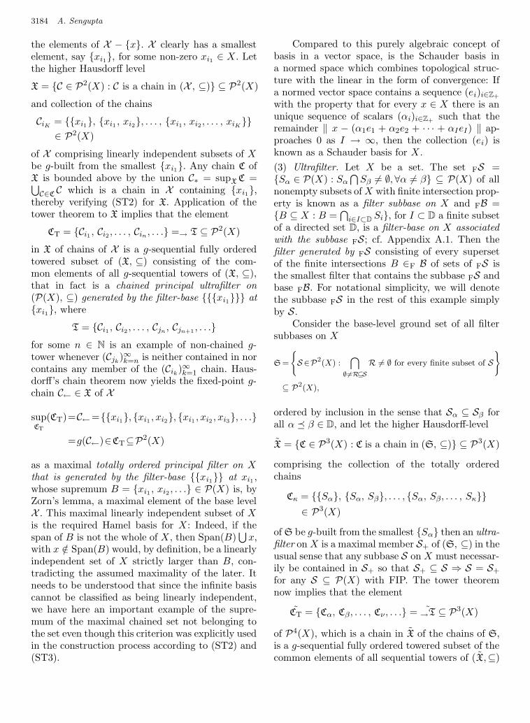
December 3, 2003 12:13 00851

3184 A. Sengupta

the elements of X − x. X clearly has a smallestelement, say xi1, for some non-zero xi1 ∈ X. Letthe higher Hausdorff level

X = C ∈ P2(X) : C is a chain in (X , ⊆) ⊆ P2(X)

and collection of the chains

CiK = xi1, xi1 , xi2, . . . , xi1 , xi2 , . . . , xiK∈ P2(X)

of X comprising linearly independent subsets of Xbe g-built from the smallest xi1. Any chain C ofX is bounded above by the union C∗ = supX C =⋃

C∈CC which is a chain in X containing xi1,

thereby verifying (ST2) for X. Application of thetower theorem to X implies that the element

CT = Ci1 , Ci2 , . . . , Cin , . . . =→ T ⊆ P2(X)

in X of chains of X is a g-sequential fully orderedtowered subset of (X, ⊆) consisting of the com-mon elements of all g-sequential towers of (X, ⊆),that in fact is a chained principal ultrafilter on(P(X), ⊆) generated by the filter-base xi1 atxi1, where

T = Ci1 , Ci2 , . . . , Cjn , Cjn+1, . . .

for some n ∈ N is an example of non-chained g-tower whenever (Cjk

)∞k=n is neither contained in norcontains any member of the (Cik)∞k=1 chain. Haus-dorff’s chain theorem now yields the fixed-point g-chain C← ∈ X of X

supCT

(CT)=C←=xi1, xi1 , xi2, xi1 , xi2 , xi3, . . .

=g(C←)∈CT⊆P2(X)

as a maximal totally ordered principal filter on Xthat is generated by the filter-base xi1 at xi1 ,whose supremum B = xi1 , xi2 , . . . ∈ P(X) is, byZorn’s lemma, a maximal element of the base levelX . This maximal linearly independent subset of Xis the required Hamel basis for X: Indeed, if thespan of B is not the whole of X, then Span(B)

⋃

x,with x /∈ Span(B) would, by definition, be a linearlyindependent set of X strictly larger than B, con-tradicting the assumed maximality of the later. Itneeds to be understood that since the infinite basiscannot be classified as being linearly independent,we have here an important example of the supre-mum of the maximal chained set not belonging tothe set even though this criterion was explicitly usedin the construction process according to (ST2) and(ST3).

Compared to this purely algebraic concept ofbasis in a vector space, is the Schauder basis ina normed space which combines topological struc-ture with the linear in the form of convergence: Ifa normed vector space contains a sequence (ei)i∈Z+

with the property that for every x ∈ X there is anunique sequence of scalars (αi)i∈Z+

such that theremainder ‖ x − (α1e1 + α2e2 + · · · + αIeI) ‖ ap-proaches 0 as I → ∞, then the collection (ei) isknown as a Schauder basis for X.

(3) Ultrafilter. Let X be a set. The set FS =Sα ∈ P(X) : Sα

⋂

Sβ 6= ∅,∀α 6= β ⊆ P(X) of allnonempty subsets ofX with finite intersection prop-erty is known as a filter subbase on X and FB =B ⊆ X : B =

⋂

i∈I⊂D Si, for I ⊂ D a finite subsetof a directed set D, is a filter-base on X associatedwith the subbase FS; cf. Appendix A.1. Then thefilter generated by FS consisting of every supersetof the finite intersections B ∈F B of sets of FS isthe smallest filter that contains the subbase FS andbase FB. For notational simplicity, we will denotethe subbase FS in the rest of this example simplyby S.

Consider the base-level ground set of all filtersubbases on X

S =

S∈P2(X) :⋂

∅6=R⊆S

R 6= ∅ for every finite subset of S

⊆ P2(X),

ordered by inclusion in the sense that Sα ⊆ Sβ forall α β ∈ D, and let the higher Hausdorff-level

X = C ∈ P3(X) : C is a chain in (S, ⊆) ⊆ P3(X)

comprising the collection of the totally orderedchains

Cκ = Sα, Sα, Sβ, . . . , Sα, Sβ, . . . , Sκ∈ P3(X)

of S be g-built from the smallest Sα then an ultra-filter onX is a maximal member S+ of (S, ⊆) in theusual sense that any subbase S on X must necessar-ily be contained in S+ so that S+ ⊆ S ⇒ S = S+

for any S ⊆ P(X) with FIP. The tower theoremnow implies that the element

CT = Cα, Cβ, . . . , Cν , . . . = →T ⊆ P3(X)

of P4(X), which is a chain in X of the chains of S,is a g-sequential fully ordered towered subset of thecommon elements of all sequential towers of (X,⊆)

December 3, 2003 12:13 00851

Toward a Theory of Chaos 3185

that is a chained principal ultrafilter on (P2(X),⊆)generated by the filter-base Sα at Sα, where

T = Cα,Cβ, . . . ,Cσ,Cς , . . .,is an obvious example of non-chained g-tower when-ever (Cσ) is neither contained in, nor contains, anymember of the Cα-chain. Hausdorff’s chain theoremnow yields the fixed-point C← ∈ X

supCT

(CT) = C← = Sα, Sα, Sβ, Sα, Sβ, Sγ, . . .

= g(C←) ∈ CT ⊆ P3(X)

as a maximal totally ordered g-chained towered sub-set of X that is, by Zorn’s lemma, a maximal ele-ment of the base level subset S of P2(X). C← isa chained principal ultrafilter on (P(X),⊆) gener-ated by the filter-base Sα at Sα, while S+ =Sα, Sβ, Sγ , . . . ∈ P2(X) is an (non-principal) ul-trafilter on X — characterized by the property thatany collection of subsets on X with FIP (that is anyfilter subbase on X) must be contained in the max-imal set S+ having FIP — that is not a principalfilter unless Sα is a singleton set xα.

What emerges from these applications of Zorn’sLemma is the remarkable fact that infinities (thedot-dot-dots) can be formally introduced as “limit-ing cases” of finite systems in a purely set-theoreticcontext without the need for topologies, metrics orconvergences. The significance of this observationwill become clear from our discussions on filters andtopology leading to Sec. 4.2 below. Also, the obser-vation on the successive iterates of the power setsP(X) in the examples above was to suggest theiranticipated role in the complex evolution of a dy-namical system that is expected to play a significantpart in our future interpretation and understandingof this adaptive and self-organizing phenomenon ofnature.

End Tutorial 5

From the examples in Tutorial 5, it should be clearthat the sequential steps summarized in Fig. 10 areinvolved in an application of Zorn’s lemma to showthat a partially ordered set has a maximal elementwith respect to its order. Thus for a partially or-dered set (X, ), form the set X of all chains C inX. If C+ is a maximal chain of X obtained by theHausdorff Maximal Principle from the chain C ofall chains of X, then its supremum u is a maximal

element of (X, ). This sequence is now applied, asin Example 4.2(1), to the set of arbitrary relationsMulti(X) on an infinite set X in order to formulateour definition of chaos that follows.

Let f be a noninjective map in Multi(X) andP (f) the number of injective branches of f . Denoteby

F = f ∈ Multi(X) : f is a noninjective function

on X ⊆ Multi(X)

the resulting basic collection of noninjective func-tions in Multi(X).

(i) For every α in some directed set D, let F havethe extension property

(∀fα ∈ F )(∃fβ ∈ F ) : P (fα) ≤ P (fβ)

(ii) Let a partial order on Multi(X) be defined,for fα, fβ ∈ Map(X) ⊆ Multi(X) by

P (fα) ≤ P (fβ) ⇔ fα fβ, (54)

with P (f) := 1 for the smallest f , define a par-tially ordered subset (F, ) of Multi(X). Thisis actually a preorder on Multi(X) in whichfunctions with the same number of injectivebranches are equivalent to each other.

(iii) Let

Cν = fα ∈ Multi(X) : fα fν ∈ P(F ) ,

ν ∈ D ,

be g-chains of non-injective functions ofMulti(X) and

X =C ∈ P(F ) : C is a chain in (F,)⊆P(F )

denote the corresponding Hausdorff level of allchains of F , with

CT = Cα, Cβ, . . . , Cν , . . . =→ T ⊆ P(F )

being a g-sequential in X . By Hausdorff Max-imal Principle, there is a maximal fixed-pointg-towered chain C← ∈ X of F

supCT

(CT) = C← = fα, fβ, . . .

= g(C←) ∈ CT ⊆ P(F ).

Zorn’s Lemma applied to this maximal chain yieldsits supremum as the maximal element of C←, andthereby of F . It needs to be appreciated, as in thecase of the algebraic Hamel basis, that the exis-tence of this maximal non-functional element was

December 3, 2003 12:13 00851

3186 A. Sengupta

obtained purely set theoretically as the “limit” of anet of functions with increasing nonlinearity, with-out resorting to any topological arguments. Becauseit is not a function, this supremum does not be-long to the functional g-towered chain having itas a fixed point, and this maximal chain does notpossess a largest, or even a maximal, element, al-though it does have a supremum.24 The supremumis a contribution of the inverse functional relations(f−α ) in the following sense. From Eq. (2), the netof increasingly non-injective functions of Eq. (54)implies a corresponding net of increasingly multi-valued functions ordered inversely by the inverserelation fα fβ ⇔ f−β f−α . Thus the inverse re-lations which are as much an integral part of graph-ical convergence as are the direct relations, have asmallest element belonging to the multifunctionalclass. Clearly, this smallest element as the requiredsupremum of the increasingly non-injective towerof functions defined by Eq. (54), serves to completethe significance of the tower by capping it with a“boundary” element that can be taken to bridge theclasses of functional and non-functional relationson X.

We are now ready to define a maximally ill-posed problem f(x) = y for x, y ∈ X in terms of amaximally non-injective map f as follows.

Definition 4.1 (Chaotic map). Let A be a non-empty closed set of a compact Hausdorff space X. Afunction f ∈ Multi(X) equivalently the sequence offunctions (fi) is maximally non-injective or chaoticon A with respect to the order relation (54) if

(a) for any fi on A there exists an fj on A satisfyingfi fj for every j > i ∈ N.

(b) the set D+ consists of a countable collection ofisolated singletons.

Definition 4.2 (Maximally ill-posed problem).Let A be a non-empty closed set of a compact Haus-dorff space X and let f be a functional relation inMulti(X). The problem f(x) = y is maximally ill-posed at y if f is chaotic on A.

As an example of the application of these def-initions, on the dense set D+, the tent map sat-isfies both the conditions of sensitive dependenceon initial conditions and topological transitivity

[Devaney, 1989] and is also maximally non-injective;the tent map is therefore chaotic on D+. In con-trast, the examples of Secs. 1 and 2 are not chaoticas the maps are not topologically transitive, al-though the Liapunov exponents, as in the case ofthe tent map, are positive. Here the (fn) are iden-tified with the iterates of f, and the “fixed point”as one through which graphs of all the functions onresidual index subsets pass. When the set of pointsD+ is dense in [0, 1] and both D+ and [0, 1]−D+ =[0, 1]−⋃∞i=0 f

−i(Per(f)) (where Per(f) denotes theset of periodic points of f) are totally disconnected,it is expected that at any point on this complementthe behavior of the limit will be similar to that onD+: these points are special as they tie up the iter-ates on Per(f) to yield the multifunctions. There-fore in any neighborhood U of a D+-point, thereis an x0 at which the forward orbit f i(x0)i≥0 ischaotic in the sense that

(a) the sequence neither diverges nor does it con-verge in the image space of f to a periodic orbitof any period, and

(b) the Liapunov exponent is given by

λ(x0)def= lim

n→∞ln

∣

∣

∣

∣

dfn(x0)

dx

∣

∣

∣

∣

1/n

= limn→∞

1

n

n−1∑

i=0

ln

∣

∣

∣

∣

df(xi)

dx

∣

∣

∣

∣

, xi = f i(x0) ,

which is a measure of the average slope of an orbitat x0 or equivalently of the average loss of informa-tion of the position of a point after one iteration, ispositive. Thus an orbit with positive Liapunov expo-nent is chaotic if it is not asymptotic (that is neitherconvergent nor adherent, having no convergent sub-orbit in the sense of Appendix A.1) to an unstableperiodic orbit or to any other limit set on which thedynamics is simple. A basic example of a chaoticorbit is that of an irrational in [0, 1] under the shiftmap and that of the chaotic set its closure, the fullunit interval.

Let f ∈ Map((X, U)) and suppose that A =f j(x0)j∈N is a sequential set corresponding to theorbit Orb(x0) = (f j(x0))j∈N, and let fRi

(x0) =⋃

j≥i fj(x0) be the i-residual of the sequence

(f j(x0))j∈N, with FBx0= fRi

(x0) : Res(N) → X

24A similar situation arises in the following more intuitive example. Although the subset A = 1/nn∈Z+of the interval

I = [−1, 1] has no smallest or minimal elements, it does have the infimum 0. Likewise, although A is bounded below by anyelement of [−1, 0), it has no greatest lower bound in [−1, 0)

⋃

(0, 1].

December 3, 2003 12:13 00851

Toward a Theory of Chaos 3187

for all i ∈ N being the decreasingly nested filter-base associated with Orb(x0). The so-called ω-limitset of x0 given by

ω(x0)def= x∈X : (∃nk∈N)(nk→∞)(fnk(x0)→x)= x ∈ X : (∀N ∈ Nx)(∀fRi

∈F Bx0)

(fRi(x0)

⋂

N 6= ∅) (55)

is simply the adherence set adh(f j(x0)) of the se-quence (f j(x0))j∈N, see Eq. (A.39); hence Defini-tion A.1.11 of the filter-base associated with a se-quence and Eqs. (A.16), (A.24), (A.31) and (A.34)allow us to express ω(x0) more meaningfully as

ω(x0) =⋂

i∈N

Cl(fRi(x0)) . (56)

It is clear from the second of Eqs. 55) that fora continuous f and any x ∈ X, x ∈ ω(x0) im-plies f(x) ∈ ω(x0) so that the entire orbit of xlies in ω(x0) whenever x does imply that the ω-limit set is positively invariant; it is also closed be-cause the adherent set is a closed set according toTheorem A.1.3. Hence x0 ∈ ω(x0) ⇒ A ⊆ ω(x0)reduces the ω-limit set to the closure of A with-out any isolated points, A ⊆ Der(A). In termsof Eq. (A.33) involving principal filters, Eq. (56)in this case may be expressed in the more trans-parent form ω(x0) =

⋂

Cl(FP(f j(x0)∞j=0)) where

the principal filter FP(f j(x0)∞j=0) at A consists

of all supersets of A = f j(x0)∞j=0, and ω(x0) rep-resents the adherence set of the principal filter atA, see the discussion following Theorem A.1.3. IfA represents a chaotic orbit under this condition,then ω(x0) is sometimes known as a chaotic set[Alligood et al., 1997]; thus the chaotic orbit in-finitely often visits every member of its chaoticset25 which is simply the ω-limit set of a chaoticorbit that is itself contained in its own limit set.Clearly the chaotic set is positive invariant, andfrom Theorem A.1.3 and its corollary it is also com-pact. Furthermore, if all (sub)sequences emanatingfrom points x0 in some neighborhood of the set con-verge to it, then ω(x0) is called a chaotic attractor,see [Alligood et al., 1997]. As common examples ofchaotic sets that are not attractors mention may bemade of the tent map with a peak value larger than1 at 0.5, and the logistic map with λ ≥ 4 again witha peak value at 0.5 exceeding 1.

It is important that the difference in the dy-namical behavior of the system on D+ and its com-plement be appreciated. At any fixed point x of f i

in D+ (or at its equivalent images in [x]) the dynam-ics eventually gets attached to the (equivalent) fixedpoint, and the sequence of iterates converges graph-ically in Multi(X) to x (or its equivalent points).When x /∈ D+, however, the orbit A = f i(x)i∈N

is chaotic in the sense that (f i(x)) is not asymp-totically periodic and not being attached to anyparticular point they wander about in the closedchaotic set ω(x) = Der(A) containing A such thatfor any given point in the set, some subsequence ofthe chaotic orbit gets arbitrarily close to it. Suchsequences do not converge anywhere but only fre-quent every point of Der(A). Thus although in thelimit of progressively larger iterations there is com-plete uncertainty of the outcome of an experimentconducted at either of these two categories of ini-tial points, whereas on D+ this is due to a randomchoice from a multifunctional set of equally prob-able outputs as dictated by the specific conditionsunder which the experiment was conducted at thatinstant, on its complement the uncertainty is dueto the chaotic behavior of the functional iteratesthemselves. Nevertheless it must be clearly under-stood that this later behavior is entirely due to themultifunctional limits at the D+ points which com-pletely determine the behavior of the system on itscomplement. As an explicit illustration of this sit-uation, recall that for the shift map 2xmod(1) theD+ points are the rationals on [0, 1], and any ir-rational is represented by a non-terminating andnon-repeating decimal so that almost all decimalsin [0, 1] in any base contain all possible sequencesof any number of digits. For the logistic map, thesituation is more complex, however. Here the on-set of chaos marking the end of the period dou-bling sequence at λ∗ = 3.5699456 is signaled by thedisappearance of all stable fixed points, Fig. 13(c),with Fig. 13(a) being a demonstration of the sta-ble limits for λ = 3.569 that show up as conver-gence of the iterates to constant valued functions(rather than as constant valued inverse functions)at stable fixed points, shown more emphatically inFig. 12(a). What actually happens at λ∗ is shown inFig. 16(a) in the next subsection: the almost verti-cal lines produced at a large, but finite, iterations i

25How does this happen for A = f i(x0)i∈N that is not the constant sequence (x0) at a fixed point? As i ∈ N increases,points are added to x0, f(x0), . . . , fI (x0) not, as would be the case in a normal sequence, as a piled-up Cauchy tail, but aspoints generally lying between those already present; recall a typical graph as of Fig. 9, for example.

December 3, 2003 12:13 00851

3188 A. Sengupta

1

0.7

(a) (b)

2

6

3

7

0

11

1

0.20 1

9

52

1

Graphical limit at 9001

Stable 1-cycle, λ = 2.95

10

Graphical limit at 9001-9002

Stable 2-cycle, λ = 3.4

1

(a)

1

0.7

(a) (b)

2

6

3

7

0

11

1

0.20 1

9

52

1

Graphical limit at 9001

Stable 1-cycle, λ = 2.95

10

Graphical limit at 9001-9002

Stable 2-cycle, λ = 3.4

1

(b)

6

8

10

5

1

2

Stable 4-cycle, λ = 3.5

Graphical limit at 9001-9004

1

0

Graphical limit at 9001-9008

Stable 8-cycle, λ = 3.55

0.7 1 0.7

1

9

0 1

1

(c)

6

8

10

5

1

2

Stable 4-cycle, λ = 3.5

Graphical limit at 9001-9004

1

0

Graphical limit at 9001-9008

Stable 8-cycle, λ = 3.55

0.7 1 0.7

1

9

0 1

1

(d)

Fig. 12. Fixed points and cycles of logistic map. The isolated fixed point of (b) yields two non-fixed points to which theiterates converge simultaneously in the sense that the generated sequence converges to one iff it converges to the other. Thissuggests that nonlinear dynamics of a system can lead to a situation in which sequences in a Hausdorff space may convergeto more than one point. Since convergence depends on the topology (Corollary to Theorem A.1.5), this may be interpretedto mean that nonlinearity tends to modify the basic structure of a space. The sequence of points generated by the iterates ofthe map are marked on the y-axis of (a)–(c) in italics. The singletons x are ω-limit sets of the respective fixed point x andis generated by the constant sequence (x, x, . . .). Whereas in (a) this is the limit of every point in (0, 1), in the other casesthese fixed points are isolated in the sense of Definition 2.3. The isolated points, however, give rise to sequences that convergeto more than one point in the form of limit cycles as shown in (b)–(d).

(the multifunctions are generated only in the limit-ing sense of i → ∞ and represent a boundary be-tween functional and non-functional relations on aset), decrease in magnitude with increasing itera-tions until they reduce to points. This gives rise toa (totally disconnected) Cantor set on the y-axis incontrast with the connected intervals that the mul-tifunctional limits at λ > λ∗ of Figs. 16(b)–16(d)produce. By our characterization Definition 4.1 of

chaos therefore, λx(1 − x) is chaotic for the valuesof λ > λ∗ that are shown in Fig. 16. We return tothis case in the following subsection.

As an example of chaos in a noniterative sys-tem, we investigate the following question: Whilemaximality of non-injectiveness produced by an in-creasing number of injective branches is necessaryfor a family of functions to be chaotic, is this alsosufficient for the system to be chaotic? This is an

December 3, 2003 12:13 00851

Toward a Theory of Chaos 3189

(a) (b).473

.5

1

1Order at λ = 3.569

Iterate 9000 of logistic map

at λ = 3.569

9000 iterations on logistic map

0.488 0.1

.507

1

(a)(a) (b)

.473

.5

1

1Order at λ = 3.569

Iterate 9000 of logistic map

at λ = 3.569

9000 iterations on logistic map

0.488 0.1

.507

1

(b)

(c) (d)

.511 1

Iterate 9000 of logistic map 9000 iterations on logistic map

at λ∗ = 3.56994560.10 1.472.493

.487‘‘Edge of chaos” at λ = λ∗

1

(c) (c) (d)

.511 1

Iterate 9000 of logistic map 9000 iterations on logistic map

at λ∗ = 3.56994560.10 1.472.493

.487”Edge of chaos” at λ = λ∗

1

(d)

(f)(e).472

.511

.493Chaos at λ = 3.57

Iterate 9000 of logistic map

.487 0

1

9000 iterations on logistic map

at λ = 3.570.1 1

1

(e)(f)(e)

.472

.511

.493Chaos at λ = 3.57

Iterate 9000 of logistic map

.487 0

1

9000 iterations on logistic map

at λ = 3.570.1 1

1

(f)

Fig. 13. Multifunctional and cobweb plots of λx(1− x). Comparison of the graphs for the three values of λ shown in (a)–(f)illustrates how the dramatic changes in the character of the former are conspicuously absent in the conventional plots thatdisplay no perceptible distinction between the three cases.

December 3, 2003 12:13 00851

3190 A. Sengupta

important question especially in the context of anon-iterative family of functions where fixed pointsare no longer relevant.

Consider the sequence of functions| sin(πnx)|∞n=1. The graphs of the subsequence| sin(2n−1πx)| and of the sequence (tn(x)) on [0, 1]are qualitatively similar in that they both contain2n−1 of their functional graphs each on a base of1/2n−1. Thus both | sin(2n−1πx)|∞n=1 and (tn(x))∞n=1converge graphically to the multifunction [0,1] onthe same set of points equivalent to 0. This is suf-ficient for us to conclude that | sin(2n−1πx)|∞n=1,and hence | sin(πnx)|∞n=1, is chaotic on the infiniteequivalent set [0]. While Fig. 9 was a comparisonof the first four iterates of the tent and absolutesine maps, Fig. 14 shows the “converged” graphicallimits after 17 iterations.

4.1. The chaotic attractor

One of the most fascinating characteristics of chaosin dynamical systems is the appearance of attrac-tors the dynamics on which are chaotic. For a subsetA of a topological space (X, U) such that R(f(A))is contained in A — in this section, unless otherwisestated to the contrary, f(A) will denote the graphand not the range (image) of f — which ensuresthat the iteration process can be carried out in A,let

fRi(A) =

⋃

j≥i∈N

f j(A)

=⋃

j≥i∈N

(

⋃

x∈A

f j(x)

)

(57)

generate the filter-base FB with Ai := fRi(A) ∈F B

being decreasingly nested, Ai+1 ⊆ Ai for all i ∈ N,in accordance with Definition A.1.1. The existenceof a maximal chain with a corresponding maxi-mal element as asssured by the Hausdorff MaximalPrinciple and Zorn’s Lemma respectively implies anonempty core of FB. As in Sec. 3 following Defi-nition 3.3, we now identify the filterbase with theneighborhood base at f∞ which allows us to define

Atr(A1)def= adh(FB)

=⋂

Ai∈FB

Cl(Ai)(58)

as the attractor of the set A1, where the last equal-ity follows from Eqs. (59) and (20) and the closureis wth respect to the topology induced by the neigh-borhood filter base FB. Clearly the attractor as de-fined here is the graphical limit of the sequence of

functions (f i)i∈N which may be verified by referenceto Definition A.1.8, Theorem A.1.3 and the proofsof Theorems A.1.4 and A.1.5, together with the di-rected set Eq. (A.10) with direction (A.11). Thebasin of attraction of the attractor is A1 becausethe graphical limit (D+, F (D+))

⋃

(G(R+), R+) ofDefinition 3.1 may be obtained, as indicated above,by a proper choice of sequences associated withA. Note that in the context of iterations of func-tions, the graphical limit (D+, y0) of the sequence(fn(x)) denotes a stable fixed point x∗ with im-age x∗ = f(x∗) = y0 to which iterations start-ing at any point x ∈ D+ converge. The graphi-cal limits (xi0,R+) are generated with respect tothe class xi∗ of points satisfying f(xi0) = xi∗,i = 0, 1, 2, . . . equivalent to unstable fixed pointx∗ := x0∗ to which inverse iterations starting at anyinitial point in R+ must converge. Even though onlyx∗ is inverse stable, an equivalent class of graph-ically converged limit multis is produced at everymember of the class xi∗ ∈ [x∗], resulting in the far-reaching consequence that every member of the classis as significant as the parent fixed point x∗ fromwhich they were born in determining the dynam-ics of the evolving system. The point to rememberabout infinite intersections of a collection of setshaving finite intersection property, as in Eq. (58), isthat this may very well be empty; recall, however,that in a compact space this is guaranteed not to beso. In the general case, if core(A) 6= ∅ then A is theprincipal filter at this core, and Atr(A1) by Eqs. (58)and (A.33) is the closure of this core, which in thiscase of topology being induced by the filterbase, isjust the core itself. A1 by its very definition, is a pos-itively invariant set as any sequence of graphs con-verging to Atr(A1) must be eventually in A1: theentire sequence therefore lies in A1. Clearly, fromTheorem A.3.1 and its corollary, the attractor is apositively invariant compact set. A typical attrac-tor is illustrated by the derived sets in the secondcolumn of Fig. 22 which also illustrates that the setof functional relations are open in Multi(X); specifi-cally functional–non-functional correspondences areneutral-selfish related as in Fig. 22, 3–2, with theattracting graphical limit of Eq. (58) forming theboundary of (finitely) many-to-one functions andthe one-to-(finitely) many multifunctions.

Equation (58) is to be compared with the im-age definition of an attractor [Stuart & Humphries,1996] where f(A) denotes the range and not thegraph of f . Then Eq. (58) can be used to define a

December 3, 2003 12:13 00851

Toward a Theory of Chaos 3191

.0008 .0008

(b)(a)

0 Graph of | sin(216πx)|17th iterate of tent map0

1 1

1

(a)

.0008 .0008

(b)(a)

0 Graph of | sin(216πx)|17th iterate of tent map0

1 1

1

(b)

Fig. 14. Similarity in the behavior of the graphs of (a) tent and (b) | sin(216πx)| maps at 17 iterations demonstrate chaoticityof the latter.

sequence of points xk ∈ Ankand hence the subset

ω(A)def= x ∈ X : (∃nk ∈ N)(nk → ∞)(∃xk ∈ Ank

)

(fnk(xk) → x)= x ∈ X : (∀N ∈ Nx)(∀Ai ∈ A)

(N⋂

Ai 6= ∅) (59)

as the corresponding attractor of A that satisfies anequation formally similar to (58) with the differencethat the filter-base A is now in terms of the imagef(A) of A, which allows the adherence expressionto take the particularly simple form

ω(A) =⋂

i∈N

Cl(f i(A)) . (60)

The complimentary subset excluded from this def-inition of ω(A), as compared to Atr(A1), that isrequired to complete the formalism is given byEq. (61) below. Observe that the equation for ω(A)is essentially Eq. (A.15), even though we prefer touse the alternate form of Eq. (A.16) as this bringsout more clearly the frequenting nature of the se-quence. The basin of attraction

Bf (A) = x ∈ A : ω(x) ⊆ Atr(A)= x ∈ A : (∃nk ∈ N)(nk → ∞)

(fnk(x) → x∗ ∈ ω(A))

(61)

of the attractor is the smallest subset of X in whichsequences generated by f must eventually lie in or-der to adhere at ω(A). Comparison of Eqs. (62)with (33) and (61) with (32) show that ω(A) can

be identified with the subset R+ on the y-axis onwhich the multifunctional limits G : R+ → X ofgraphical convergence are generated, with its basinof attraction being contained in the D+ associatedwith the injective branch of f that generates R+. Insummary it may be concluded that since definitions(59) and (61) involve both the domain and rangeof f , a description of the attractor in terms of thegraph of f , like that of Eq. (58), is more pertinentand meaningful as it combines the requirements ofboth these equations. Thus, for example, as ω(A) isnot the function G(R+), this attractor does not in-clude the equivalence class of inverse stable pointsthat may be associated with x∗, see for exampleFig. 15.

From Eq. (59), we may make the particularlysimple choice of (xk) to satisfy fnk(x−k) = x sothat x−k = f−nk

B (x), where x−k ∈ [x−k] := f−nk(x)is the element of the equivalence class of the inverseimage of x corresponding to the injective branch fB.This choice is of special interest to us as it is theclass that generates the G-function on R+ in graph-ical convergence. This allows us to express ω(A) as

ω(A) = x ∈ X : (∃nk ∈ N)(nk → ∞)(f−nk

B (x)

= x−kconverges in (X, U)) ; (62)

note that the x−k of this equation and the xk ofEq. (59) are, in general, quite different points.

A simple illustrative example of the construc-tion of ω(A) for the positive injective branch ofthe homeomorphism (4x2 − 1)/3, −1 ≤ x ≤ 1, is

December 3, 2003 12:13 00851

3192 A. Sengupta

3

3

0.8

0.4

0.2

0.6

−0.4 −0.2 0.2 0.60.4−0.6 0 0.8−0.8

x−1 x

−3

f2

B

f3

B

x1 x2

x

1

−0.25

x−1

fB

f =4x2

− 1

3

−0.4

1

245

124

1

Fig. 15. The attractor for f(x) = (4x2 − 1)/3, for −1 ≤ x ≤ 1. The converging sequences are denoted by arrows on theright, and (xk) are chosen according to the construction shown. This example demonstrates how although A ⊆ f(A), whereA = [0, 1] is the domain of the positive injective branch of f , the succeeding images (f i(A))i≥1 satisfy the required restrictionfor iteration, and A in the discussion above can be taken to be f(A); this is permitted as only a finite number of iteratesis thereby discarded. It is straightforward to verify that Atr(A1) = (−1, [−0.25, 1])

⋃

((−1, 1), −0.25)⋃

(1, [−0.25, 1]) withF (x) = −0.25 on D− = (−1, 1) = D+ and G(y) = 1, and −1 on R− = [−0.25, 1] = R+. By comparison, ω(A) from eitherits definition Eq. (59) or from the equivalent intersection expression Eq. (60), is simply the closed interval R+ = [−0.25, 1].The italicized iterate numbers on the graphs show how the oscillations die out with increasing iterations from x = ±1 andapproach −0.25 in all neighborhoods of 0.

shown in Fig. 15, where the arrow-heads denote theconverging sequences fni(xi) → x and fni−m(xi) →x−m which proves invariance of ω(A) for a homeo-morphic f ; here continuity of the function and itsinverse is explicitly required for invariance. Posi-tive invariance of a subset A of X implies that forany n ∈ N and x ∈ A, fn(x) = yn ∈ A, whilenegative invariance assures that for any y ∈ A,f−n(y) = x−n ∈ A. Invariance of A in both theforward and backward directions therefore meansthat for any y ∈ A and n ∈ N, there exists a x ∈ Asuch that fn(x) = y. In interpreting this figure, itmay be useful to recall from Definition 4.1 that anincreasing number of injective branches of f is anecessary, but not sufficient, condition for the oc-currence of chaos; thus in Figs. 12(a) and 15, in-creasing noninjectivity of f leads to constant valuedlimit functions over a connected D+ in a mannersimilar to that associated with the classical Gibb’sphenomenon in the theory of Fourier series.

Graphical convergence of an increasingly non-linear family of functions implied by its increasingnon-injectivity may now be combined with the re-

quirements of an attractor to lead to the concept ofa chaotic attractor to be that on which the dynam-ics is chaotic in the sense of Definitions 4.1. and 4.2.Hence

Definition 4.3 (Chaotic Attractor). Let A be apositively invariant subset of X. The attractorAtr(A) is chaotic on A if there is sensitive depen-dence on initial conditions for all x ∈ A. The sensi-tive dependence manifests itself as multifunctionalgraphical limits for all x ∈ D+ and as chaotic orbitswhen x 6∈ D+.

The picture of chaotic attractors that emergefrom the foregoing discussions and our characteri-zation of chaos of Definition 4.1 is that it it is asubset of X that is simultaneously “spiked” multi-functional on the y-axis and consists of a dense col-lection of singleton domains of attraction on the x-axis. This is illustrated in Fig. 16 which shows sometypical chaotic attractors. The first four diagrams(a)–(d) are for the logistic map with (b)–(d) show-ing the 4-, 2- and 1-piece attractors for λ = 3.575,

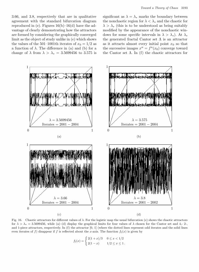
December 3, 2003 12:13 00851

Toward a Theory of Chaos 3193

3.66, and 3.8, respectively that are in qualitativeagreement with the standard bifurcation diagramreproduced in (e). Figures 16(b)–16(d) have the ad-vantage of clearly demonstrating how the attractorsare formed by considering the graphically convergedlimit as the object of study unlike in (e) which showsthe values of the 501–1001th iterates of x0 = 1/2 asa function of λ. The difference in (a) and (b) for achange of λ from λ > λ∗ = 3.5699456 to 3.575 is

significant as λ = λ∗ marks the boundary betweenthe nonchaotic region for λ < λ∗ and the chaotic forλ > λ∗ (this is to be understood as being suitablymodified by the appearance of the nonchaotic win-dows for some specific intervals in λ > λ∗). At λ∗the generated fractal Cantor set Λ is an attractoras it attracts almost every initial point x0 so thatthe successive images xn = fn(x0) converge towardthe Cantor set Λ. In (f) the chaotic attractors for

(a) (b)1

1

0

1

1 0

λ = 3.5699456

Iterates = 2001 − 2004

λ = 3.575

Iterates = 2001 − 2004

1

(a)(a) ----

1

1

0

1

1 0

λ = 3.5699456

Iterates = 2001 − 2004

λ = 3.575

Iterates = 2001 − 2004

1

(b)

(c) (d)

λ = 3.66

Iterates = 2001 − 2004

λ = 3.8

Iterates = 2001 − 2002

1

1

00 1

1

1

(c) (c)

λ = 3.66

Iterates = 2001 − 2004

λ = 3.8

Iterates = 2001 − 2002

1

1

00 1

1

1

(d)

Fig. 16. Chaotic attractors for different values of λ. For the logistic map the usual bifurcation (e) shows the chaotic attractorsfor λ > λ∗ = 3.5699456, while (a)–(d) display the graphical limits for four values of λ chosen for the Cantor set and 4,- 2-,and 1-piece attractors, respectively. In (f) the attractor [0, 1] (where the dotted lines represent odd iterates and the solid lineseven iterates of f) disappear if f is reflected about the x-axis. The function ff (x) is given by

ff(x) =

2(1 + x)/3 0 ≤ x < 1/2

2(1 − x) 1/2 ≤ x ≤ 1 .

December 3, 2003 12:13 00851

3194 A. Sengupta

(e) (f)

First 12 iterates0 0

1

1λ4 λ∗ 4

λ4 = 3.449

1

1

(e) (e) (f)

First 12 iterates0 0

1

1λ4 λ∗ 4

λ4 = 3.449

1

1

(f)

Fig. 16. (Continued )

the piecewise continuous function on [0, 1]

ff(x) =

2(1 + x)

3, 0 ≤ x <

1

2

2(1 − x),1

2≤ x ≤ 1 ,

is [0, 1] where the dotted lines represent odd iteratesand the full lines even iterates of f ; here the attrac-tor disappears if the function is reflected about thex-axis.

4.2. Why chaos? A preliminary

inquiry

The question as to why a natural system shouldevolve chaotically is both interesting and relevant,and this section attempts to advance a plausible an-swer to this inquiry that is based on the connectionbetween topology and convergence contained in theCorollary to Theorem A.1.5. Open sets are group-ings of elements that govern convergence of netsand filters, because the required property of beingeither eventually or frequently in (open) neighbor-hoods of a point determines the eventual behaviorof the net; recall in this connection the unusual con-vergence characteristics in cofinite and cocountablespaces. Conversely for a given convergence charac-teristic of a class of nets, it is possible to infer thetopology of the space that is responsible for thisconvergence, and it is this point of view that weadopt here to investigate the question of this sub-section: recall that our Definitions 4.1 and 4.2 werebased on purely algebraic set-theoretic arguments

on ordered sets, just as the role of the choice ofan appropriate problem-dependent basis was high-lighted at the end of Sec. 2. Chaos as manifest in itsattractors is a direct consequence of the increasingnonlinearity of the map with increasing iteration;we reemphasize that this is only a necessary condi-tion so that the increasing nonlinearities of Figs. 12and 15 eventually lead to stable states and not tochaotic instability. Under the right conditions asenunciated following Fig. 10, chaos appears to bethe natural outcome of the difference in the behav-ior of a function f and its inverse f− under theirsuccessive applications. Thus f = ff−f allows fto take advantage of its multi-inverse to generateall possible equivalence classes that are available, afeature not accessible to f− = f−ff−. As we haveseen in the foregoing, equivalence classes of fixedpoints, stable and unstable, are of defining signif-icance in determining the ultimate behavior of anevolving dynamical system and as the eventual (asalso frequent) charcter of a filter or net in a setis dictated by open neighborhoods of points of theset, it is postulated that chaoticity on a set X leadsto a reformulation of the open sets of X to equiv-alence classes generated by the evolving map f , seeExample 2.4(3). Such a redefinition of open sets ofequivalence clases allow the evolving system to tem-porally access an ever increasing number of stateseven though the equivalent fixed points are not fixedunder iterations of f except for the parent of theclass, and can be considered to be the governingcriterion for the cooperative or collective behavior

December 3, 2003 12:13 00851

Toward a Theory of Chaos 3195

of the system. The predominance of the role of f−

in f = ff−f in generating the equivalence classes(that is exploiting the many-to-one character) of fis reflected as limit multis for f (i.e. constant f−

on R+) in f− = f−ff−; this interpretation of thedynamics of chaos is meaningful as graphical con-vergence leading to chaos is a result of pointwise bi-convergence of the sequence of iterates of the func-tions generated by f . But as f is a noninjectivefunction on X possessing the property of increasingnonlinearity in the form of increasing noninjectivitywith iteration, various cycles of disjoint equivalenceclasses are generated under iteration, see for exam-ple Fig. 9(a) for the tent map. A reference to Fig.shows that the basic set XB, for a finite number n ofiterations of f , contains the parent of each of theseopen equivalent sets in the domain of f , with thetopology on XB being the corresponding p-imagesof these disjoint saturated open sets of the domain.In the limit of infinite iterations of f leading to themultifunction M (this is the f∞ of Sec. 4.1), thegenerated open sets constitute a basis for a topol-ogy on D(f) and the basis for the topology of R(f)are the corresponding M-images of these equivalentclasses. It is our contention that the motive force be-hind evolution toward a chaos, as defined by Defini-tion 4.1, is the drive toward a state of the dynamicalsystem that supports ininality of the limit multi M;see Appendix A.2 with the discussions on Fig. andEq. (26) in Sec. 2. In the limit of infinite iterationstherefore, the open sets of the range R(f) ⊆ X arethe multi images that graphical convergence gener-ates at each of these inverse-stable fixed points. Xtherefore has two topologies imposed on it by thedynamics of f : the first of equivalence classes gen-erated by the limit multi M in the domain of f andthe second as M-images of these classes in the rangeof f . Quite clearly these two topologies need not bethe same; their intersection therefore can be definedto be the chaotic topology on X associated with thechaotic map f onX. Neighborhoods of points in thistopology cannot be arbitrarily small as they consistof all members of the equivalence class to whichany element belongs; hence a sequence convergingto any of these elements necessarily converges toall of them, and the eventual objective of chaoticdynamics is to generate a topology in X with re-spect to which elements of the set can be groupedtogether in as large equivalence classes as possiblein the sense that if a net converges simultaneously

to points x 6= y ∈ X then x ∼ y: x is of courseequivalent to itself while x, y, z are equivalent toeach other iff they are simultaneously in every openset in which the net may eventually belong. Thishall-mark of chaos can be appreciated in terms ofa necessary obliteration of any separation propertythat the space might have originally possessed, seeproperty (H3) in Appendix A.3. We reemphasizethat a set in this chaotic context is required to actin a dual capacity depending on whether it carriesthe initial or final topology under M.

This preliminary inquiry into the nature ofchaos is concluded in the final section of this paper.

5. Graphical Convergence Works

We present in this section some real evidence insupport of our hypothesis of graphical conver-gence of functions in Multi(X,Y ). The example istaken from neutron transport theory, and concernsthe discretized spectral approximation [Sengupta,1988, 1995] of Case’s singular eigenfunction solu-tion of the monoenergetic neutron transport equa-tion, [Case & Zweifel, 1967]. The neutron transportequation is a linear form of the Boltzmann equationthat is obtained as follows. Consider the neutron-moderator system as a mixture of two species ofgases each of which satisfies a Boltzmann equationof the type(

∂

∂t+ vi · ∇

)

fi(r, v, t)

=

∫

dv′∫

dv1

∫

dv′1∑

j

Wij(vi → v′; v1 → v′1)

fi(r, v′, t)fj(r, v

′1, t) − fi(r, v, t)fj(r, v1, t)

where

Wij(vi → v′; v1 → v′1) = |v − v1|σij(v − v′, v1 − v′1)

σij being the cross-section of interaction betweenspecies i and j. Denote neutrons by subscript 1 andthe background moderator with which the neutronsinteract by 2, and make the assumptions that

(i) The neutron density f1 is much less comparedwith that of the moderator f2 so that the termsf1f1 and f1f2 may be neglected in the neutron andmoderator equations, respectively.

(ii) The moderator distribution f2 is not affectedby the neutrons. This decouples the neutron andmoderator equations and leads to an equilibrium

December 3, 2003 12:13 00851

3196 A. Sengupta

Maxwellian fM for the moderator while the neu-trons are described by the linear equation(

∂

∂t+ v · ∇

)

f(r, v, t)

=

∫

dv′∫

dv1

∫

dv′1W12(v → v′; v1 → v′1)

f(r, v′, t)fM(v′1) − f(r, v, t)fM(v1))This is now put in the standard form of the neutrontransport equation [Williams, 1971](

1

v

∂

∂t+ Ω · v + S(E)

)

Φ(r, E, Ω, t)

=

∫

dΩ′∫

dE′S(r, E′ → E; Ω′ · Ω)Φ(r, E′, Ω′, t).

where E = mv2/2 is the energy and Ω the direc-tion of motion of the neutrons. The steady state,monoenergetic form of this equation is Eq. (A.53)

µ∂Φ(x, µ)

∂x+ Φ(x, µ) =

c

2

∫ 1

−1Φ(x, µ′)dµ′ ,

0 < c < 1, −1 ≤ µ ≤ 1

and its singular eigenfunction solution for x ∈(−∞, ∞) is given by Eq. (A.56)

Φ(x, µ) = a(ν0)e−x/ν0φ(µ, ν0)

+ a(−ν0)ex/ν0φ(−ν0, µ)

+

∫ 1

−1a(ν)e−x/νφ(µ, ν)dν ;

see Appendix A.4 for an introductory review ofCase’s solution of the one-speed neutron transportequation.

The term “eigenfunction” is motivated by thefollowing considerations. Consider the eigenvalueequation

(µ− ν)Fν(µ) = 0, µ ∈ V (µ), ν ∈ R (63)

in the space of multifunctions Multi(V (µ), (−∞,∞)), where µ is in either of the intervals [−1, 1]or [0, 1] depending on whether the given bound-ary conditions for Eq. (A.53) is full-range or halfrange. If we are looking only for functional solu-tions of Eq. (63), then the unique function F thatsatisfies this equation for all possible µ ∈ V (µ) andν ∈ R− V (µ) is Fν(µ) = 0 which means, accordingto Table 1, that the point spectrum of µ is emptyand (µ−ν)−1 exists for all ν. When ν ∈ V (µ), how-ever, this inverse is not continuous and we showbelow that in Map(V (µ), 0), ν ∈ V (µ) belongs to

the continuous spectrum of µ. This distinction be-tween the nature of the inverses depending on therelative values of µ and ν suggests a wider “non-function” space in which to look for the solutions ofoperator equations, and in keeping with the philos-ophy embodied in Fig. of treating inverse prob-lems in the space of multifunctions, we considerall Fν ∈ Multi(V (µ), R)) satisfying Eq. (63) to beeigenfunctions of µ for the corresponding eigenvalueν, leading to the following multifunctional solutionof (63)

Fν(µ) =

(V (µ), 0) if ν /∈ V (µ)

(V (µ) − ν, 0)⋃

(ν, R)) if ν ∈ V (µ) ,

where V (µ)−ν is used as a shorthand for the inter-val V (µ) with ν deleted. Rewriting the eigenvalueequation (63) as µν(Fν(µ)) = 0 and comparing thiswith Fig. , allows us to draw the correspondences

f ⇔ µν

X and Y ⇔ Fν ∈ Multi(V (µ), R) :

Fν ∈ D(µν)f(X) ⇔ 0 : 0 ∈ Y XB ⇔ 0 : 0 ∈ Xf− ⇔ µ−ν .

(64)

Thus a multifunction in X is equivalent to 0 in XB

under the linear map µν , and we show below thatthis multifunction is in fact the Dirac delta “func-tion” δν(µ), usually written as δ(µ − ν). This sug-gests that in Multi(V (µ), R), every ν ∈ V (µ) is inthe point spectrum of µ, so that discontinuous func-tions that are pointwise limits of functions in func-tion space can be replaced by graphically convergedmultifunctions in the space of multifunctions. Com-pleting the equivalence class of 0 in Fig. , gives themultifunctional solution of Eq. (63).

From a comparison of the definition of ill-posedness (Sec. 2) and the spectrum (Table 1), it isclear that Lλ(x) = y is ill-posed iff

(1) Lλ not injective ⇔ λ ∈ Pσ(Lλ), which corre-sponds to the first row of Table 1.

(2) Lλ not surjective ⇔ the values of λ correspondto the second and third columns of Table 1.

(3) Lλ is bijective but not open ⇔ λ is either inCσ(Lλ) or Rσ(Lλ) corresponding to the secondrow of Table 1.

We verify in the three steps below that X =L1[−1, 1] of integrable functions, ν ∈ V (µ) = [−1, 1]belongs to the continuous spectrum of µ.

December 3, 2003 12:13 00851

Toward a Theory of Chaos 3197

Table 1. Spectrum of linear operator L ∈ Map(X). Here Lλ := L−λ satisfiesthe equation Lλ(x) = 0, with the resolvent set ρ(L) of L consisting of all thosecomplex numbers λ for which L−1

λexists as a continuous operator with dense

domain. Any value of λ for which this is not true is in the spectrum σ(L)of L, that is further subdivided into three disjoint components of the point,continuous and residual spectra according to the criteria shown in the table.

R(Lλ)

Lλ L−1λ

R = X Cl(R) = X Cl(R) 6= X

Not injective · · · Pσ(L) Pσ(L) Pσ(L)

InjectiveNot continuous Cσ(L) Cσ(L) Rσ(L)

Continuous ρ(L) ρ(L) Rσ(L)

(a) R(µν) is dense, but not equal to L1. The setof functions g(µ) ∈ L1 such that µ−1

ν g ∈ L1

cannot be the whole of L1. Thus, for example,the piecewise constant function g = const 6= 0on |µ − ν| ≤ δ > 0 and 0 otherwise is in L1

but not in R(µν) as µ−1ν g 6∈ L1. Nevertheless

for any g ∈ L1, we may choose the sequence offunctions

gn(µ) =

0, if |µ− ν| ≤ 1/n

g(µ), otherwise

in R(µν) to be eventually in every neighbor-

hood of g in the sense that limn→∞

∫ 1−1 |g −

gn| = 0.(b) The inverse (µ− ν)−1 exists but is not contin-

uous. The inverse exists because, as noted ear-lier, 0 is the only functional solution of Eq. (63).

Nevertheless although the net of functions

δνε(µ) =1

tan−1(1 + ν)/ε+ tan−1(1 − ν)/ε

×(

ε

(µ− ν)2 + ε2

)

, ε > 0

is in the domain of µν because∫ 1−1 δνε(µ)dµ = 1

for all ε > 0,

limε→0

∫ 1

−1|µ− ν|δνε(µ)dµ = 0

implying that (µ− ν)−1 is unbounded.Taken together, (a) and (b) show that func-

tional solutions of Eq. (63) lead to state 2–2 inTable 1; hence ν ∈ [−1, 1] = Cσ(µ).

(c) The two integral constraints in (b) also meanthat ν ∈ Cσ(µ) is a generalized eigenvalueof µ which justifies calling the graphical limit

δνε(µ)G→ δν(µ) a generalized, or singular, eigen-

(b)(a)

−32

0

−0.5

0.5

0.5

20

0

−32

1

(a)(b)(a)

−32

−0.50

−0.5

0.5

20

0

32

1

(b)

Fig. 17. Graphical convergence of: (a) Poisson kernel δε(x) = ε/π(x2 + ε2) and (b) conjugate Poisson kernel Pε(x) =x/(x2 + ε2) to the Dirac delta and principal value, respectively; the graphs, each for a definite ε-value, converges to therespective limits as ε → 0.

December 3, 2003 12:13 00851

3198 A. Sengupta

function, see Fig. 17 which clearly indicates theconvergence of the net of functions.26

From the fact that the solution Eq. (A.56) ofthe transport equation contains an integral involv-ing the multifunction φ(µ, ν), we may draw an in-teresting physical interpretation. As the multi ap-pears everywhere on V (µ) (i.e. there are no chaoticorbits but only the multifunctions that producethem), we have here a situation typical of maximalill-posedness characteristic of chaos: note that boththe functions comprising φε(µ, ν) are non-injective.As the solution (A.56) involves an integral over allν ∈ V (µ), the singular eigenfunctions — that col-lectively may be regarded as representing a chaoticsubstate of the system represented by the solution ofthe neutron transport equation — combine with thefunctional components φ(±ν0, µ) to produce thewell-defined, non-chaotic, experimental end resultof the neutron flux Φ(x, µ).

The solution (A.56) is obtained by assumingΦ(x, µ) = e−x/νφ(µ, ν) to get the equation forφ(µ, ν) to be (µ− ν)φ(µ, ν) = −cν/2 with the nor-

malization∫ 1−1 φ(µ, ν) = 1. As µ−1

ν is not invert-ible in Multi(V (µ), R) and µνB : XB → f(X) doesnot exist, the alternate approach of regularizationwas adopted in [Sengupta, 1988, 1995] to rewriteµνφ(µ, ν) = −cν/2 as µνεφε(µ, ν) = −cν/2 withµνε := µ − (ν + iε) being a net of bijective func-tions for ε > 0; this is a consequence of the factthat for the multiplication operator every non-realλ belongs to the resolvent set of the operator. Thefamily of solutions of the latter equation is given by[Sengupta 1988, 1995]

φε(ν, µ) =cν

2

ν − µ

(µ− ν)2 + ε2+λε(ν)

πε

ε

(µ− ν)2 + ε2

(65)

where the required normalization∫ 1−1 φε(ν, µ) = 1

gives

λε(ν) =πε

tan−1(1 + ν)/ε+ tan−1(1 − ν)/ε

×(

1 − cν

4ln

(1 + ν)2 + ε2

(1 − ν)2 + ε2

)

ε→0−→ πλ(ν)

with

πε = ε

∫ 1

−1

dµ

µ2 + ε2= 2 tan−1

(

1

ε

)

ε→0−→ π .

These discretized equations should be comparedwith the corresponding exact ones of Appendix A.4.We shall see that the net of functions (65) con-verges graphically to the multifunction Eq. (A.55)as ε→ 0.

In the discretized spectral approximation,the singular eigenfunction φ(µ, ν) is replaced byφε(µ, ν), ε→ 0, with the integral in ν being replacedby an appropriate sum. The solution Eq. (A.58) ofthe physically interesting half-space x ≥ 0 problemthen reduces to [Sengupta, 1988, 1995]

Φε(x, µ) = a(ν0)e−x/ν0φ(µ, ν0)

+

N∑

i=1

a(νi)e−x/νiφε(µ, νi) µ ∈ [0, 1]

(66)

where the nodes νiNi=1 are chosen suitably. This

discretized spectral approximation to Case’s so-lution has given surprisingly accurate numericalresults for a set of properly chosen nodes whencompared with exact calculations. Because of itsinvolved nature [Case & Zweifel, 1967], the exactcalculations are basically numerical which leads tononlinear integral equations as part of the solu-tion procedure. To appreciate the enormous com-plexity of the exact treatment of the half-spaceproblem, we recall that the complete set of eigen-functions φ(µ, ν0), φ(µ, ν)ν∈[0,1] are orthogo-nal with respect to the half-range weight functionW (µ) of half-range theory, Eq. (A.61), that is ex-pressed only in terms of solution of the nonlin-ear integral equation Eq. (A.62). The solution ofa half-space problem then evaluates the coefficientsa(ν0), a(ν)ν∈[0, 1] from the appropriate half range(that is 0 ≤ µ ≤ 1) orthogonality integrals satisfiedby the eigenfunctions φ(µ, ν0), φ(µ, ν)ν∈[0, 1]with respect to the weight W (µ), see Appendix A.4for the necessary details of the half-space problemin neutron transport theory.

As may be appreciated from this brief introduc-tion, solutions to half-space problems are not sim-ple and actual numerical computations must rely agreat deal on tabulated values of the X-function.

26The technical definition of a generalized eigenvalue is as follows. Let L be a linear operator such that there exists in thedomain of L a sequence of elements (xn) with ‖xn‖ = 1 for all n. If limn→∞ ‖(L − λ)xn‖ = 0 for some λ ∈ C, then this λ isa generalized eigenvalue of L, the corresponding eigenfunction x∞ being a generalized eigenfunction.

December 3, 2003 12:13 00851

Toward a Theory of Chaos 3199

Self-consistent calculations of sample benchmarkproblems performed by the discretized spectral ap-proximation in a full-range adaption of the half-range problem described below that generate allnecessary data, independent of numerical tables,with the quadrature nodes νiN

i=1 taken at thezero Legendre polynomials show that the full rangeformulation of this approximation [Sengupta, 1988,1995] can give very accurate results not only of inte-grated quantities like the flux Φ and leakage of par-ticles out of the half space, but of also basic “raw”data like the extrapolated end point

z0 =cν0

4

∫ 1

0

ν

N(ν)

(

1 +cν2

1 − ν2

)

ln

(

ν0 + ν

ν0 − ν

)

dν

(67)

and of the X-function itself. Given the involved

nature of the exact theory, it is our contention thatthe remarkable accuracy of these basic data, someof which is reproduced in Table 2, is due to thegraphical convergence of the net of functions

φε(µ, ν)G→ φ(µ, ν)

shown in Fig. 18; here ε = 1/πN so that ε → 0as N → ∞. By this convergence, the deltafunction and principal values in [−1, 1] are themultifunctions ([−1, 0), 0)

⋃

(0, [0, ∞)⋃

((0, 1], 0)and 1/xx∈[−1, 0)

⋃

(0, (−∞, ∞))⋃1/xx∈(0, 1]

respectively. Tables 2 and 3, taken from [Sengupta,1988] and [Sengupta, 1995], show respectively theextrapolated end point and X-function by thefull-range adaption of the discretized spectral ap-proximation for two different half-range problemsdenoted as Problems A and B defined as

(b)(a)

c = 0.3 c = 0.9

c = 0.3 c = 0.9N = 1000 N = 1000

1

(a) (b)(a)

c = 0.3 c = 0.9

c = 0.3 c = 0.9N = 1000 N = 1000

1

(b)

Fig. 18. Rational function approximations φε(µ, ν) of the singular eigenfunction φ(µ, ν) at four different values of ν. N = 1000denotes the “converged” multifunction φ, with the peaks at the specific ν-values chosen.

December 3, 2003 12:13 00851

3200 A. Sengupta

Problem A Equation : µΦx + Φ = (c/2)∫ 1−1 Φ(x, µ′)dµ′, x ≥ 0

Boundary condition : Φ(0, µ) = 0 for µ ≥ 0

Asymptotic condition : Φ → e−x/ν0φ(µ, ν0) as x→ ∞ .

P roblem B Equation : µΦx + Φ = (c/2)∫ 1−1 Φ(x, µ′)dµ′, x ≥ 0

Boundary condition : Φ(0, µ) = 1 for µ ≥ 0

Asymptotic condition : Φ → 0 as x→ ∞ .

The full −1 ≤ µ ≤ 1 range form of the half0 ≤ µ ≤ 1 range discretized spectral approxima-tion replaces the exact integral boundary conditionat x = 0 by a suitable quadrature sum over the val-ues of ν taken at the zeros of Legendre polynomials;thus the condition at x = 0 can be expressed as

ψ(µ) = a(ν0)φ(µ, ν0) +

N∑

i=1

a(νi)φε(µ, νi) ,

µ ∈ [0, 1] ,

(68)

where ψ(µ) = Φ(0, µ) is the specified incomingradiation incident on the boundary from the left,and the half-range coefficients a(ν0), a(ν)ν∈[0,1]

are to be evaluated using the W -function ofAppendix A.4. We now exploit the relative sim-plicity of the full-range calculations by replacingEq. (68) by Eq. (69) following, where the coefficientsb(νi)N

i=0 are used to distinguish the full-range co-efficients from the half-range ones. The significanceof this change lies in the overwhelming simplicity

of the full-range weight function µ as compared tothe half-range functionW (µ), and the resulting sim-plicity of the orthogonality relations that follow, seeAppendix A.4. The basic data of z0 and X(−ν)are then completely generated self-consistently[Sengupta, 1988, 1995] by the discretized spectralapproximation from the full-range adaption

N∑

i=0

biφε(µ, νi) = ψ+(µ) + ψ−(µ) ,

µ ∈ [−1, 1], νi ≥ 0

(69)

Table 2. Extrapolated end-point z0.

cz0

c N = 2 N = 6 N = 10 Exact

0.2 0.78478 0.78478 0.78478 0.78510.4 0.72996 0.72996 0.72996 0.73050.6 0.71535 0.71536 0.71536 0.71550.8 0.71124 0.71124 0.71124 0.71130.9 0.71060 0.71060 0.71061 0.7106

Table 3. X(−ν) by the full-range method.

X(−ν)

c N νi Problem A Problem B Exact

0.2 20.2133 0.8873091 0.8873091 0.8873080.7887 0.5826001 0.5826001 0.582500

0.0338 1.3370163 1.3370163 1.3370150.1694 1.0999831 1.0999831 1.099983

0.6 60.3807 0.8792321 0.8792321 0.879232

0.6193 0.7215240 0.7215240 0.7215240.8306 0.6239109 0.6239109 0.6239110.9662 0.5743556 0.5743556 0.574355

0.0130 1.5971784 1.5971784 1.5971630.0674 1.4245314 1.4245314 1.4245320.1603 1.2289940 1.2289940 1.2289950.2833 1.0513750 1.0513750 1.051376

0.9 100.4255 0.9058140 0.9058410 0.905842

0.5744 0.7934295 0.7934295 0.7934300.7167 0.7102823 0.7102823 0.7102830.8397 0.6516836 0.6516836 0.6516830.9325 0.6136514 0.6136514 0.6136530.9870 0.5933988 0.5933988 0.593399

December 3, 2003 12:13 00851

Toward a Theory of Chaos 3201

of the discretized boundary condition Eq. (68),where ψ+(µ) is by definition the incident flux ψ(µ)for µ ∈ [0, 1] and 0 if µ ∈ [−1, 0], while

ψ−(µ) =

N∑

i=0

b−i φε(µ, νi) if µ ∈ [−1, 0], νi ≥ 0

0 if µ ∈ [0, 1]

is the emergent angular distribution out of themedium. Equation (69) corresponds to the full-range µ ∈ [−1, 1], νi ≥ 0 form

b(ν0)φ(µ, ν0) +

∫ 1

0b(ν)φ(µ, ν)dν

= ψ+(µ) +

(

b−(ν0)φ(µ, ν0) +

∫ 1

0b−(ν)φ(µ, ν)dν

)

(70)

of boundary condition (A.59) with the first and sec-ond terms on the right having the same interpre-tation as for Eq. (69). This full-range simulationmerely states that the solution (A.58) of Eq. (A.53)holds for all µ ∈ [−1, 1], x ≥ 0, although it was ob-tained, unlike in the regular full-range case, fromthe given radiation ψ(µ) incident on the bound-ary at x = 0 over only half the interval µ ∈ [0, 1].To obtain the simulated full-range coefficients biand b−i of the half-range problem, we observe thatthere are effectively only half the number of coef-ficients as compared to a normal full-range prob-lem because ν is now only over half the full inter-val. This allows us to generate two sets of equationsfrom (70) by integrating with respect to µ ∈ [−1, 1]with ν in the half intervals [−1, 0] and [0, 1] toobtain the two sets of coefficients b− and b, re-spectively. Accordingly we get from Eq. (69) withj = 0, 1, . . . , N the sets of equations

(ψ, φj−)(+)µ = −

N∑

i=0

b−i (φi+, φj−)(−)µ

bj =1

Nj

(

(ψ, φj+)(+)µ +

N∑

i=0

b−i (φi+, φj+)(−)µ

)

(71)

where (φj±)Nj=1 represents (φε(µ,±νj))Nj=1, φ0± =

φ(µ, ±ν0), the (+) (−) superscripts are used todenote the integrations with respect to µ ∈ [0, 1]and µ ∈ [−1, 0] respectively, and (f, g)µ denotesthe usual inner product in [−1, 1] with respectto the full range weight µ. While the first set ofN + 1 equations give b−i , the second set produces

the required bj from these “negative” coefficients.By equating these calculated bi with the exact half-range expressions for a(ν) with respect to W (µ) asoutlined in Appendix A.4, it is possible to find nu-merical values of z0 and X(−ν). Thus from the sec-ond of Eq. (A.64), X(−νi)N

i=1 is obtained withbiB = aiB, i = 1, . . . , N , which is then substitutedin the second of Eq. (A.63) with X(−ν0) obtainedfrom aA(ν0) according to Appendix A.4, to comparethe respective aiA with the calculated biA from (71).Finally the full-range coefficients of Problem A canbe used to obtain the X(−ν) values from the sec-ond of Eqs. (A.63) and compared with the exacttabulated values as in Table 3. The tabulated val-ues of cz0 from Eq. (67) show a consistent deviationfrom our calculations of Problem A according toaA(ν0) = − exp(−2z0/ν0). Since the X(−ν) valuesof Problem A in Table 3 also need the same b0A asinput that was used in obtaining z0, it is reasonableto conclude that the “exact” numerical integrationof z0 is inaccurate to the extent displayed in Table 2.

From these numerical experiments and Fig. 18we may conclude that the continuous spectrum[−1, 1] of the position operator µ acts as the D+

points in generating the multifunctional Case sin-gular eigenfunction φ(µ, ν). Its rational approxima-tion φε(µ, ν) in the context of the simple simulatedfull-range computations of the complex half-rangeexact theory of Appendix A.4, clearly demonstratesthe utility of graphical convergence of sequence offunctions to multifunction. The totality of the mul-tifunctions φ(µ, ν) for all ν in Figs. 18(c) and 18(d)endows the problem with the character of max-imal ill-posedness that is characteristic of chaos.This chaotic signature of the transport equation ishowever latent as the experimental output Φ(x, µ)is well-behaved and regular. This important exam-ple shows how nature can use hidden and complexchaotic substates to generate order through a pro-cess of superposition.

6. Does Nature Support

Complexity?

The question of this section is basic in the light ofthe theory of chaos presented above as it may bereformulated to the inquiry of what makes naturesupport chaoticity in the form of increasing non-injectivity of an input–output system. It is the pur-pose of this section to exploit the connection be-tween spectral theory and the dynamics of chaosthat has been presented in the previous section.

December 3, 2003 12:13 00851

3202 A. Sengupta

Since linear operators on finite dimensional spacesdo not possess continuous or residual spectra, spec-tral theory on infinite dimensional spaces essentiallyinvolves limiting behavior to infinite dimensions ofthe familiar matrix eigenvalue–eigenvector problem.As always this means extensions, dense embeddingsand completions of the finite dimensional problemthat show up as generalized eigenvalues and eigen-vectors. In its usual form, the goal of nonlinear spec-tral theory consists [Appell et al., 2000] in the studyof T−1

λ for nonlinear operators Tλ that satisfy moregeneral continuity conditions, like differentiabilityand Lipschitz continuity, than simple boundednessthat is sufficient for linear operators. The followinggeneralization of the concept of the spectrum of alinear operator to the nonlinear case is suggestive.For a nonlinear map, λ need not appear only in amultiplying role, so that an eigenvalue equation canbe written more generally as a fixed-point equation

f(λ; x) = x

with a fixed point corresponding to the eigenfunc-tion of a linear operator and an “eigenvalue” beingthe value of λ for which this fixed point appears.The correspondence of the residual and continu-ous parts of the spectrum are, however, less trivialthan for the point spectrum. This is seen from thefollowing two examples [Roman, 1975]. Let Aek =λkek, k = 1, 2, . . . be an eigenvalue equation withej being the jth unit vector. Then (A − λ)ek :=(λk − λ)ek = 0 iff λ = λk so that λk∞k=1 ∈ Pσ(A)are the only eigenvalues of A. Consider now (λk)

∞k=1

to be a sequence of real numbers that tends toa finite λ∗; for example, let A be a diagonal ma-trix having 1/k as its diagonal entries. Then λ∗

belongs to the continuous spectrum of A because(A − λ∗)ek = (λk − λ∗)ek with λk → λ∗ impliesthat (A − λ∗)−1 is an unbounded linear operatorand λ∗ a generalized eigenvalue of A. In the secondexample Aek = ek+1/(k + 1), it is not difficult toverify that: (a) The point spectrum of A is empty,(b) The range of A is not dense because it doesnot contain e1, and (c) A−1 is unbounded becauseAek → 0. Thus the generalized eigenvalue λ∗ = 0 inthis case belongs to the residual spectrum of A. Ineither case, limj→∞ ej is the corresponding general-ized eigenvector that enlarges the trivial null spaceN (Lλ∗) of the generalized eigenvalue λ∗. In factin these two and the Dirac delta example of Sec.5 of continuous and residual spectra, the general-ized eigenfunctions arise as the limits of a sequence

of functions whose images under the respective Lλ

converge to 0; recall the definition of footnote 26.This observation generalizes to the dense extensionMulti|(X, Y ) of Map(X, Y ) as follows. If x ∈ D+

is not a fixed point of f(λ; x) = x, but there issome n ∈ N such that fn(λ; x) = x, then the limitn → ∞ generates a multifunction at x as was thecase with the delta function in the previous sectionand the various other examples that we have seenso far in the earlier sections.

One of the main goals of investigations on thespectrum of nonlinear operators is to find a set inthe complex plane that has the usual desirable prop-erties of the spectrum of a linear operator [Appellet al., 2000]. In this case, the focus has been to finda suitable class of operators C(X) with T ∈ C(X),such that the resolvent set is expressed as

ρ(T ) = λ ∈ C : (Tλ is 1 : 1)(Cl(R(Tλ) = X)

and (T−1λ ∈ C(X) on R(Tλ))

with the spectrum σ(T ) being defined as the com-plement of this set. Among the classes C(X) thathave been considered, beside spaces of continu-ous functions C(X), are linear boundedness B(X),Frechet differentiability C1(X), Lipschitz continu-ity Lip(X), and Granas quasiboundedness Q(x),where Lip(X) specifically takes into account thenonlinearity of T to define

‖T‖Lip = supx6=y‖T (x) − T (y)‖

‖x− y‖ ,

|T |lip = infx6=y =‖T (x) − T (y)‖

‖x− y‖

(72)

that are plain generalizations of the correspondingnorms of linear operators. Plots of f−λ (y) = x ∈D(f−λ) : (f−λ)x = y for the functions f : R → R

fλa(x) =

−1 − λx, x < −1(1 − λ)x, −1 ≤ x ≤ 11 − λx, 1 < x

fλb(x) =

−λx, x < 1(1 − λ)x− 1, 1 ≤ x ≤ 21 − λx, 2 < x

fλc(x) =

−λx x < 1√x− 1 − λx 1 ≤ x

fλd(x) =

(x− 1)2 + 1 − λx 1 ≤ x ≤ 2(1 − λ)x otherwise

fλe(x) = tan−1(x) − λx

December 3, 2003 12:13 00851

Toward a Theory of Chaos 3203

5

3

−1

−3

0

1

2

−1

0

2

1

−1

4

−5

1 0

4−4

−2

−10

2

0.5

1

12

10−10

1

−10

10

(c)

0.5 −0.5

−0.5

−0.5

(b)

−1

1 02

3

−1

0

(f)

−4 5

−1

10

00.5

1

1.5

2

−0.5

1.5

−12

(a)

(d)

−1

0.50

(e)

0

2

10

−1

2 −1

−0.5 0.5 1 1.5

2

3−3

0

3

2

(a)

5

3

−1

−3

0

1

2

−1

0

2

1

−1

4

−5

1 0

4−4

−2

−10

2

0.5

1

12

10−10

1

−10

10

(c)

0.5 −0.5

−0.5

−0.5

(b)

−1

1 02

3

−1

0

(f)

−4 5

−1

10

00.5

1

1.5

2

−0.5

1.5

−12

(a)

(d)

−1

0.50

(e)

0

2

10

−1

2 −1

−0.5 0.5 1 1.5

2

3−3

0

3

2

(b)

5

3

−1

−3

0

1

2

−1

0

2

1

−1

4

−5

1 0

4−4

−2

−10

2

0.5

1

12

10−10

1

−10

10

(c)

0.5 −0.5

−0.5

−0.5

(b)

−1

1 02

3

−1

0

(f)

−4 5

−1

10

00.5

1

1.5

2

−0.5

1.5

−12

(a)

(d)

−1

0.50

(e)

0

2

10

−1

2 −1

−0.5 0.5 1 1.5

2

3−3

0

3

2

(c)

5

3

−1

−3

0

1

2

−1

0

2

1

−1

4

−5

1 0

4−4

−2

−10

2

0.5

1

12

10−10

1

−10

10

(c)

0.5 −0.5

−0.5

−0.5

(b)

−1

1 02

3

−1

0

(f)

−4 5

−1

10

00.5

1

1.5

2

−0.5

1.5

−12

(a)

(d)

−1

0.50

(e)

0

2

10

−1

2 −1

−0.5 0.5 1 1.5

2

3−3

0

3

2

(d)

5

3

−1

−3

0

1

2

−1

0

2

1

−1

4

−5

1 0

4−4

−2

−10

2

0.5

1

12

10−10

1

−10

10

(c)

0.5 −0.5

−0.5

−0.5

(b)

−1

1 02

3

−1

0

(f)

−4 5

−1

10

00.5

1

1.5

2

−0.5

1.5

−12

(a)

(d)

−1

0.50

(e)

0

2

10

−1

2 −1

−0.5 0.5 1 1.5

2

3−3

0

3

2

(e)

5

3

−1

−3

0

1

2

−1

0

2

1

−1

4

−5

1 0

4−4

−2

−10

2

0.5

1

12

10−10

1

−10

10

(c)

0.5 −0.5

−0.5

−0.5

(b)

−1

1 02

3

−1

0

(f)

−4 5

−1

10

00.5

1

1.5

2

−0.5

1.5

−12

(a)

(d)

−1

0.50

(e)

0

2

10

−1

2 −1

−0.5 0.5 1 1.5

2

3−3

0

3

2

(f)

Fig. 19. Inverses of fλ = f − λ. The λ-values are shown on the graphs.

fλf(x) =

1 − 2√−x− λx, x < −1

(1 − λ)x, −1 ≤ x ≤ 1

2√x− 1 − λx, 1 < x

taken from [Appell et al., 2000] are shown in Fig. 19.It is easy to verify that the Lipschitz and linearupper and lower bounds of these maps are as inTable 4.

The point spectrum defined by

Pσ(f) = λ ∈ C : (f − λ)x = 0 for some x 6= 0is the simplest to calculate. Because of the spe-cial role played by the zero element 0 in generatingthe point spectrum in the linear case, the boundsm‖x‖ ≤ ‖Lx‖ ≤ M‖x‖ together with Lx = λximply Cl(Pσ(L)) = [‖L‖b, ‖L‖B] — where thesubscripts denote the lower and upper bounds inEq. (72) and which sometimes is taken to be a de-scriptor of the point spectrum of a nonlinear op-erator — as can be seen in Table 5 and verifiedfrom Fig. 19. The remainder of the spectrum, as

the complement of the resolvent set, is more diffi-

cult to find. Here the convenient characterization of

the resolvent of a continuous linear operator as the

set of all sufficiently large λ that satisfy |λ| > M is

of little significance as, unlike for a linear operator,

the non-existence of an inverse is not just due to

the set f−1(0) which happens to be the only way

a linear map can fail to be injective. Thus the map

defined piecewise as α+ 2(1 − α)x for 0 ≤ x < 1/2

and 2(1 − x) for 1/2 ≤ x ≤ 1, with 0 < α < 1, is

not invertible on its range although f−(0) = 1.

Comparing Fig. 19 and Table 4, it is seen that in

cases (b)–(d), the intervals [|f |b, ‖f‖B] are subsets

of the λ-values for which the respective maps are

not injective; this is to be compared with (a), (e)

and (f) where the two sets are the same. Thus the

linear bounds are not good indicators of the unique-

ness properties of solution of nonlinear equations for

which the Lipschitzian bounds are seen to be more

appropriate.

December 3, 2003 12:13 00851

3204 A. Sengupta

Table 4. Bounds on the functions of Fig. 19.

Function |f |b ‖f‖B |f |lip ‖f‖Lip

fa 0 1 0 1

fb 0 1/2 0 1

fc 0 1/2 0 ∞fd 2(

√2 − 1) ∞ 0 2

fe 0 1 0 1

ff 0 1 0 1

Table 5. Lipschitzian and point spectraof the functions of Fig. 19.

Functions σLip(f) Pσ(f)

fa [0, 1] (0, 1]

fb [0, 1] [0, 1/2]

fc [0, ∞) [0, 1/2]

fd [0, 2] [2(√

2 − 1), 1]

fe [0, 1] (0, 1)

ff [0, 1] (0, 1)

In view of the above, we may draw the follow-ing conclusions. If we choose to work in the spaceof multifunctions Multi(X, T ), with T the topologyof pointwise biconvergence, when all functional re-lations are (multi)invertible on their ranges, we maymake the following definition for the net of functionsf(λ; x) satisfying f(λ; x) = x.

Definition 6.1. Let f(λ; ·) ∈ Multi(X, T ) be afunction. The resolvent set of f is given by

ρ(f) = λ : (f(λ; ·)−1 ∈ Map(X, T ))

∧(Cl(R(f(λ; ·)) = X) ,

and any λ not in ρ is in the spectrum of f .

Thus apart from multifunctions, λ ∈ σ(f) alsogenerates functions on the boundary of functionaland non-functional relations in Multi(X, T ). Whileit is possible to classify the spectrum into point,continuous and residual subsets, as in the linearcase, it is more meaningful for nonlinear opera-tors to consider λ as being either in the bound-ary spectrum Bdy(σ(f)) or in the interior spectrumInt(σ(f)), depending on whether or not the mul-tifunction f(λ; ·)− arises as the graphical limit ofa net of functions in either ρ(f) or Rσ(f). Thisis suggested by the spectra arising from the sec-ond row of Table 1 (injective Lλ and discontinu-ous L−1

λ ) that lies sandwiched in the λ-plane be-tween the two components arising from the firstand third rows, see [Naylor & Sell, 1971, Sec. 6.6],for example. According to this simple scheme, thespectral set is a closed set with its boundary andinterior belonging to Bdy(σ(f)) and Int(σ(f)), re-spectively. Table 6 shows this division for the ex-amples in Fig. 19. Because 0 is no more significantthan any other point in the domain of a nonlin-ear map in inducing non-injectivity, the division ofthe spectrum into the traditional sets would be asshown in Table 6; compare also with the conven-tional linear point spectrum of Table 5. In this non-linear classification, the point spectrum consists ofany λ for which the inverse f(λ; ·)− is set-valued,irrespective of whether this is produced at 0 or not,while the continuous and residual spectra togethercomprise the boundary spectrum. Thus a λ can beboth at the point and the continuous or residualspectra which need not be disjoint. The continuousand residual spectra are included in the boundaryspectrum which may also contain parts of the pointspectrum.

Example 6.1. To see how these concepts applyto linear mappings, consider the equation (D −λ)y(x) = r(x) where D = d/dx is the differential

Table 6. Nonlinear spectra of functions of Fig. 19. Compare the presentpoint spectra with the usual linear spectra of Table 5.

Function Int(σ(f)) Bdy(σ(f)) Pσ(f) Cσ(f) Rσ(f)

fa (0, 1) 0, 1 [0, 1] 1 0fb (0, 1) 0, 1 [0, 1] 1 0fc (0, ∞) 0 [0, ∞) 0 ∅fd (0, 2) 0, 2 (0, 2) 0, 2 ∅fe (0, 1) 0, 1 (0, 1) 1 0ff (0, 1) 0, 1 (0, 1) 0, 1 ∅

December 3, 2003 12:13 00851

Toward a Theory of Chaos 3205

operator on L2[0, ∞), and let λ be real. For λ 6= 0,the unique solution of this equation in L2[0, ∞), is

y(x) =

eλx

(

y(0) +

∫ x

0e−λx′

r(x′)dx′)

, λ < 0

eλx

(

y(0) −∫ ∞

xe−λx′

r(x′)dx′)

λ > 0

showing that for λ > 0 the inverse is functional sothat λ ∈ (0, ∞) belongs to the resolvent of D. How-ever, when λ < 0, apart from the y = 0 solution(since we are dealing with a linear problem, onlyr = 0 is to be considered), eλx is also in L2[0, ∞)so that all such λ are in the point spectrum of D.For λ = 0 and r 6= 0, the two solutions are not nec-essarily equal unless

∫∞0 r(x) = 0, so that the range

R(D − I) is a subspace of L2[0, ∞). To completethe problem, it is possible to show [Naylor & Sell,1971] that 0 ∈ Cσ(D), see Example 2.2; hence thecontinuous spectrum forms at the boundary of thefunctional solution for the resolvent-λ and the mul-tifunctional solution for the point spectrum. Witha slight variation of problem to y(0) = 0, all λ < 0are in the resolvent set, while λ > 0 the inverse isbounded but must satisfy y(0) =

∫∞0 e−λxr(x)dx =

0 so that Cl(R(D−λ)) 6= L2[0,∞). Hence λ > 0 be-long to the residual spectrum. The decompositionof the complex λ-plane for these and some otherlinear spectral problems taken from [Naylor & Sell,1971] is shown in Fig. 20. In all cases, the spectrumdue to the second row of Table 1 acts as a boundarybetween that arising from the first and third rows,which justifies our division of the spectrum for anonlinear operator into the interior and boundarycomponents. Compare with Example 2.2.

From the basic representation of the resolventoperator (1 − f)−1

1 + f + f2 + · · · + f i + · · ·in Multi(X), if the iterates of f converge to a multi-function for some λ, then that λmust be in the spec-trum of f , which means that the control parameterof a chaotic dynamical system is in its spectrum. Ofcourse, the series can sum to a multi even otherwise:take fλ(x) to be identically x with λ = 1, for exam-ple, to get 1 ∈ Pσ(f). A comparison of Tables 1 and5 reveal that in case (d), for example, 0 and 2 belongto the Lipschtiz spectrum because although f−1

d isnot Lipschitz continuous, ‖f‖Lip = 2. It should alsobe noted that the boundary between the functionalresolvent and multifunctional spectral set is formed

by the graphical convergence of a net of resolventfunctions while the multifunctions in the interior ofthe spectral set evolve graphically independent ofthe functions in the resolvent. The chaotic statesforming the boundary of the functional and multi-functional subsets of Multi(X) marks the transitionfrom the less efficient functional state to the moreefficient multifunctional one.

These arguments also suggest the following.The countably many outputs arising from the non-injectivity of f(λ; ·) corresponding to a given inputcan be interpreted to define complexity because ina nonlinear system each of these possibilities con-stitute an experimental result in itself that may notbe combined in any definite predtermined manner.This is in sharp contrast to linear systems wherea linear combination, governed by the initial con-ditions, always generate a unique end result; recallalso the combination offered by the singular gen-eralized eigenfunctions of neutron transport the-ory. This multiplicity of possibilities that have nodefinite combinatorial property is the basis of thediversity of nature, and is possibly responsible forFeigenbaum’s “historical prejudice”, [Feigenbaum,1992], see Prelude 2. Thus order represented bythe functional resolvent passes over to complexityof the countably multifunctional interior spectrumvia the uncountably multifunctional boundary thatis a prerequisite for chaos. We may now strengthenour hypothesis offered at the end of the previoussection in terms of the examples of Figs. 19 and20, that nature uses chaoticity as an intermediatestep to the attainment of states that would other-wise be inaccessible to it. Well-posedness of a sys-tem is an extremely inefficient way of expressing amultitude of possibilities as this requires a differentinput for every possible output. Nature chooses toexpress its myriad manifestations through the mul-tifunctional route leading either to averaging as inthe delta function case or to a countable set of well-defined states, as in the examples of Fig. 19 corre-sponding to the interior spectrum. Of course it is nodistraction that the multifunctional states arise re-spectively from fλ and f−λ in these examples as f isa function on X that is under the influence of bothf and its inverse. The functional resolvent is, for allpractical purposes, only a tool in this structure ofnature.

The equation f(x) = y is typically an input–output system in which the inverse images at a func-tional value y0 represents a set of input parametersleading to the same experimental output y0; this

December 3, 2003 12:13 00851

3206 A. Sengupta

Resolventset

Point

setResidual

spectrum

spectrum spectrumPoint

spectrum

spectrumspectrum

set

spectrumContinuous

set

setResolvent

set

spectrumContinuous Residual

spectrumContinuous

Resolvent

spectrumContinuous

Resolvent Resolvent

Continuous

Resolvent

Continuous

λ-plane

1

(a)

Resolventset

Point

setResidual

spectrum

spectrum spectrumPoint

spectrum

spectrumspectrum

set

spectrumContinuous

set

setResolvent

set

spectrumContinuous Residual

spectrumContinuous

Resolvent

spectrumContinuous

Resolvent Resolvent

Continuous

Resolvent

Continuous

λ-plane

1

(b)

Resolventset

Point

setResidual

spectrum

spectrum spectrumPoint

spectrum

spectrumspectrum

set

spectrumContinuous

set

setResolvent

set

spectrumContinuous Residual

spectrumContinuous

Resolvent

spectrumContinuous

Resolvent Resolvent

Continuous

Resolvent

Continuous

λ-plane

1

(c)

Resolventset

Point

setResidual

spectrum

spectrum spectrumPoint

spectrum

spectrumspectrum

set

spectrumContinuous

set

setResolvent

set

spectrumContinuous Residual

spectrumContinuous

Resolvent

spectrumContinuous

Resolvent Resolvent

Continuous

Resolvent

Continuous

λ-plane

1

(d)

Resolventset

Point

setResidual

spectrum

spectrum spectrumPoint

spectrum

spectrumspectrum

set

spectrumContinuous

set

setResolvent

set

spectrumContinuous Residual

spectrumContinuous

Resolvent

spectrumContinuous

Resolvent Resolvent

Continuous

Resolvent

Continuous

λ-plane

1

(e)

"!#

(f)

Fig. 20. Spectra of some linear operators in the complex λ-plane. (a) Left shift (. . . , x−1, x0, x1, . . .) 7→ (. . . x0, x1, x2, . . .)on l2(−∞, ∞), (b) Right shift (x0, x1, x2, . . .) 7→ (0, x0, x1, . . .) on l2[0, ∞), (c) Left shift (x0, x1, x2, . . .) 7→ (x1, x2, x3, . . .)on l2[0, ∞) of sequence spaces, and (d) d/dx on L2(−∞, ∞) (e) d/dx on L2[0, ∞) with y(0) = 0 and (f) d/dx on L2[0, ∞).The residual spectrum in (b) and (e) arise from block (3–3) in Table 1, i.e. Lλ is one-to-one and L−1

λis bounded on non-

dense domains in l2[0, ∞) and L2[0, ∞), respectively. The continuous spectrum therefore marks the boundary between twofunctional states, as in (a) and (e), now with dense and non-dense domains of the inverse operator.

is stability characterized by a complete insensitiv-ity of the output to changes in input. On the otherhand, a continuous multifunction at x0 is a signalfor a hypersensitivity to input because the output,which is a definite experimental quantity, is a choicefrom the possibly infinite set f(x0) made by achoice function which represents the experiment atthat particular point in time. Since there will alwaysbe finite differences in the experimental parameterswhen an experiment is repeated, the choice function(that is the experimental output) will select a pointfrom f(x0) that is representative of that experi-ment and which need not bear any definite relationto the previous values; this is instability and sig-nals sensitivity to initial conditions. Such a state isof high entropy as the number of available statesfC(f(x0)) — where fC is the choice function —

is larger than a functional state represented by thesingleton f(x0).

Epilogue

The most passionate advocates of the new science

go so far as to say that twentieth-century science

will be remembered for just three things: relativity,

quantum mechanics and chaos. Chaos, they contend,

has become the century’s third great revolution in

the physical sciences. Like the first two revolutions,

chaos cuts away at the tenets of Newton’s physics. As

one physicist put it: “Relativity eliminated the New-

tonian illusion of absolute space and time; quantum

theory eliminated the Newtonian dream of a con-

trollable measurement process; and chaos eliminates

the Laplacian fantasy of deterministic predictability.”

Of the three, the revolution in chaos applies to the

December 3, 2003 12:13 00851

Toward a Theory of Chaos 3207

universe we see and touch, to objects at human scale.

. . . There has long been a feeling, not always expressed

openly, that theoretical physics has strayed far from

human intuition about the world. Whether this will

prove to be fruitful heresy, or just plain heresy, no one

knows. But some of those who thought that physics

might be working its way into a corner now look to

chaos as a way out.

[Gleick, 1987]

Acknowledgments

It is a pleasure to thank the referees for recom-mending an enlarged Tutorial and Review revisionof the original submission Graphical Convergence,Chaos and Complexity, and Professor Leon O. Chuafor suggesting a pedagogically self-contained, jar-gonless version accessible to a wider audience forthe present form of the paper. Financial assis-tance during the initial stages of this work fromthe National Board for Higher Mathematics is alsoacknowledged.

References

Alligood, K. T., Sauer, T. D. & Yorke, J. A. [1997] Chaos,An Introduction to Dynamical Systems (Springer-Verlag, NY).

Appell, J., DePascale, E. & Vignoli, A. [2000] “A com-parison of different spectra for nonlinear operators,”Nonlin. Anal. 40, 73–90.

Brown, R. & Chua, L. O. [1996] “Clarifying chaos:Examples and counterexamples,” Int. J. Bifurcationand Chaos 6, 219–249.

Campbell, S. I. & Mayer, C. D. [1979] GeneralizedInverses of Linear Transformations (Pitman Publish-ing Ltd., London).

Case, K. M. & Zweifel, P. F. [1967] Linear TransportTheory (Addison-Wesley, MA).

de Souza, H. G. [1997] “Opening address,” in The Im-pact of Chaos on Science and Society, eds. Grebogi,C. & Yorke, J. A. (United Nations University Press,Tokyo), pp. 384–386.

Devaney, R. L. [1989] An Introduction to Chaotic Dy-namical Systems (Addison-Wesley, CA).

Falconer, K. [1990] Fractal Geometry (John Wiley,Chichester).

Feigenbaum, M. [1992] “Foreword,” Chaos and Fractals:New Frontiers of Science (Springer-Verlag, NY),pp. 1–7.

Gallagher, R. & Appenzeller, T. [1999] “Beyond reduc-tionism,” Science 284, p. 79.

Gleick, J. [1987] Chaos: The Amazing Science of the Un-predictable (Viking, NY).

Goldenfeld, N. & Kadanoff, L. P. [1999] “Simple lessonsfrom complexity,” Science 284, 87–89.

Korevaar, J. [1968] Mathematical Methods, Vol. 1 (Aca-demic Press, NY).

Naylor, A. W. & Sell, G. R. [1971] Linear OperatorTheory is Engineering and Science Holt (Rinehart andWinston, NY).

Peitgen, H.-O., Jurgens, H. & Saupe, D. [1992] Chaosand Fractals: New Frontiers of Science (Springer-Verlag, NY).

Robinson, C. [1999] Dynamical Systems: Stability, Sym-bolic Dynamics and Chaos (CRC Press LLC, BocaRaton).

Roman, P. [1975] Some Modern Mathematics for Physi-cists and other Outsiders (Pergammon Press, NY).

Sengupta, A. [1995a] “A discretized spectral approxima-tion in neutron transport theory. Some numerical con-siderations,” J. Stat. Phys. 51, 657–676.

Sengupta, A. [1995b] “Full range solution of half-spaceneutron transport problem,” ZAMP 46, 40–60.

Sengupta, A. [1997] “Multifunction and generalized in-verse,” J. Inverse and Ill-Posed Problems 5, 265–285.

Sengupta, A. & Ray, G. G. [2000] “A multifunctional ex-tension of function spaces: Chaotic systems are maxi-mally ill-posed,” J. Inverse and Ill-Posed Problems 8,232–353.

Stuart, A. M. & Humphries, A. R. [1996] DynamicalSystems and Numerical Analysis (Cambridge Univer-sity Press).

Tikhonov, A. N. & Arsenin, V. Y. [1977] Solutions of Ill-Posed Problems (V. H. Winston, Washington D.C.).

Waldrop, M. M. [1992] Complexity: The Emerging Sci-ence at the Edge of Order and Chaos (Simon andSchuster).

Willard, S. [1970] General Topology (Addison-Wesley,Reading, MA).

Williams, M. M. R. [1971] Mathematical Methods ofParticle Transport Theory (Butterworths, London).

Appendix

This Appendix gives a brief overview of some as-pects of topology that are necessary for a properunderstanding of the concepts introduced in thiswork.

A.1. Convergence in Topological

Spaces: Sequence, Net and

Filter

In the theory of convergence in topological spaces,countability plays an important role. To understandthe significance of this concept, some preliminariesare needed.

December 3, 2003 12:13 00851

3208 A. Sengupta

The notion of a basis, or base, is a familiar onein analysis: a base is a subcollection of a set whichmay be used to construct, in a specified manner, anyelement of the set. This simplifies the statement ofa problem since a smaller number of elements ofthe base can be used to generate the larger classof every element of the set. This philosophy findsapplication in topological spaces as follows.

Among the three properties (N1) − (N3) of theneighborhood system Nx of Tutorial 4, (N1) and(N2) are basic in the sense that the resulting sub-collection of Nx can be used to generate the fullsystem by applying (N3); this basic neighborhoodsystem, or neighborhood (local ) base Bx at x, is char-acterized by

(NB1) x belongs to each member B of Bx.

(NB2) The intersection of any two members of Bx

contains another member of Bx: B1, B2 ∈ Bx ⇒(∃B ∈ Bx : B ⊆ B1

⋂

B2).

Formally, compare Eq. (18),

Definition A.1.1. A neighborhood (local) base Bx

at x in a topological space (X, U) is a subcollectionof the neighborhood system Nx having the prop-erty that each N ∈ Nx contains some member ofBx. Thus

Bxdef= B ∈ Nx : x ∈ B ⊆ N for each N ∈ Nx

(A.1)

determines the full neighborhood system

Nx = N ⊆ X : x ∈ B ⊆ N for some B ∈ Bx(A.2)

reciprocally as all supersets of the basic elements.

The entire neighborhood system Nx, which isrecovered from the base by forming all supersets ofthe basic neighborhoods, is trivially a local base atx; non-trivial examples are given below.

The second example of a base, consisting asusual of a subcollection of a given collection, is thetopological base TB that allows the specification ofthe topology on a set X in terms of a smaller col-lection of open sets.

Definition A.1.2. A base TB in a topological space(X, U) is a subcollection of the topology U havingthe property that each U ∈ U contains some mem-ber of TB. Thus

TB def= B ∈ U : B ⊆ U for each U ∈ U (A.3)

determines reciprocally the topology U as

U =

U ⊆ X : U =⋃

B∈TB

B

. (A.4)

This means that the topology on X can be recon-structed from the base by taking all possible unionsof members of the base, and a collection of subsetsof a set X is a topological base iff Eq. (A.4) of arbi-trary unions of elements of TB generates a topologyon X. This topology, which is the coarsest (that isthe smallest) that contains TB, is obviously closedunder finite intersections. Since the open set Int(N)is a neighborhood of x whenever N is, Eq. (A.2)and the definition Eq. (17) of Nx implies that theopen neighborhood system of any point in a topo-logical space is an example of a neighborhood baseat that point, an observation that has often led, to-gether with Eq. (A.3), to the use of the term “neigh-borhood” as a synonym for “non-empty open set”.The distinction between the two however is signifi-cant as neighborhoods need not necessarily be opensets; thus while not necessary, it is clearly sufficientfor the local basic sets B to be open in Eqs. (A.1)and (A.2). If Eq. (A.2) holds for every x ∈ N , thenthe resulting Nx reduces to the topology induced bythe open basic neighborhood system Bx as given byEq. (18).

In order to check if a collection of subsets TBof X qualifies to be a basis, it is not necessary toverify properties (T1)–(T3) of Tutorial 4 for theclass (A.4) generated by it because of the proper-ties (TB1) and (TB2) below whose strong affinity to(NB1) and (NB2) is formalized in Theorem A.1.1.

Theorem A.1.1. A collection TB of subsets of Xis a topological basis on X iff

(TB1) X =⋃

B ∈T BB. Thus each x ∈ X must be-

long to some B ∈ TB which implies the existenceof a local base at each point x ∈ X.

(TB2) The intersection of any two members B1 andB2 of TB with x ∈ B1

⋂

B2 contains another mem-ber of TB: (B1, B2 ∈ TB)∧ (x ∈ B1

⋂

B2) ⇒ (∃B ∈TB : x ∈ B ⊆ B1

⋂

B2).

This theorem, together with Eq. (A.4) ensuresthat a given collection of subsets of a set X sat-isfying (TB1) and (TB2) induces some topologyon X; compared to this is the result that anycollection of subsets of a set X is a subbasisfor some topology on X. If X, however, alreadyhas a topology U imposed on it, then Eq. (A.3)

December 3, 2003 12:13 00851

Toward a Theory of Chaos 3209

must also be satisfied in order that the topol-ogy generated by TB is indeed U . The next the-orem connects the two types of bases of Defini-tions A.1.1 and A.1.2 by asserting that althougha local base of a space need not consist of opensets and a topological base need not have any ref-erence to a point of X, any subcollection of thebase containing a point is a local base at thatpoint.

Theorem A.1.2. A collection of open sets TB isa base for a topological space (X, U) iff for eachx ∈ X, the subcollection

Bx = B ∈ U : x ∈ B ∈ TB (A.5)

of basic sets containing x is a local base at x.

Proof. Necessity. Let TB be a base of (X, U) andN be a neighborhood of x, so that x ∈ U ⊆ N forsome open set U =

⋃

B ∈TBB and basic open sets

B. Hence x ∈ B ⊆ N shows, from Eq. (A.1), thatB ∈ Bx is a local basic set at x.

Sufficiency. If U is an open set of X contain-ing x, then the definition of local base Eq. (A.1)requires x ∈ Bx ⊆ U for some subcollection of basicsets Bx in Bx; hence U =

⋃

x∈U Bx. By Eq. (A.4)therefore, TB is a topological base for X.

Because the basic sets are open, (TB2) ofTheorem A.1.1 leads to the following physicallyappealing paraphrase of Theorem A.1.2.

Corollary. A collection TB of open sets of (X, U)is a topological base that generates U iff for eachopen set U of X and each x ∈ U there is an openset B ∈ TB such that x ∈ B ⊆ U ; that is iff

x ∈ U ∈ U ⇒ (∃B ∈ TB : x ∈ B ⊆ U) .

Example A.1.1. Some examples of local bases in R

are intervals of the type (x−ε, x+ε), [x−ε, x+ε] forreal ε, (x−q, x+q) for rational q, (x−1/n, x+1/n)for n ∈ Z+, while for a metrizable space with thetopology induced by a metric d, each of the follow-ing is a local base at x ∈ X: Bε(x; d) := y ∈ X :d(x, y) < ε and Dε(x; d) := y ∈ X : d(x, y) ≤ εfor ε > 0, Bq(x; d) for Q 3 q > 0 and B1/n(x; d)

for n ∈ Z+. In R2, two neighborhood bases at anyx ∈ R2 are the disks centered at x and the setof all squares at x with sides parallel to the axes.Although these bases have no elements in common,they are nevertheless equivalent in the sense thatthey both generate the same (usual) topology in

R2. Of course, the entire neighborhood system atany point of a topological space is itself a (less use-ful) local base at that point. By Theorem A.1.2,Bε(x; d), Dε(x; d), ε > 0, Bq(x; d), Q 3 q > 0 andB1/n(x; d), n ∈ Z+, for all x ∈ X are examples ofbases in a metrizable space with topology inducedby a metric d.

In terms of local bases and bases, it is now pos-sible to formulate the notions of first and secondcountability as follows.

Definition A.1.3. A topological space is firstcountable if each x ∈ X has some countable neigh-borhood base, and is second countable if it has acountable base.

Every metrizable space (X, d) is first countableas both B(x, q)Q3q>0 and B(x, 1/n)n∈Z+

areexamples of countable neighborhood bases at anyx ∈ (X, d); hence Rn is first countable. It should beclear that although every second countable spaceis first countable, only a countable first countablespace can be second countable, and a common ex-ample of an uncountable first countable space thatis also second countable is provided by Rn. Metriz-able spaces need not be second countable: any un-countable set having the discrete topology is as anexample.

Example A.1.2. The following is an important ex-ample of a space that is not first countable as it isneeded for our pointwise biconvergence of Sec. 3.Let Map(X, Y ) be the set of all functions betweenthe uncountable spaces (X, U) and (Y, V). Givenany integer I ≥ 1, and any finite collection of points(xi)

Ii=1 of X and of open sets (Vi)

Ii=1 in Y , let

B((xi)Ii=1; (Vi)

Ii=1) = g ∈ Map(X, Y ) :

(g(xi) ∈ Vi)(i = 1, 2, . . . , I)(A.6)

be the functions in Map(X,Y ) whose graphs passthrough each of the sets (Vi)

Ii=1 at (xi)

Ii=1, and

let TB be the collection of all such subsets ofMap(X, Y ) for every choice of I, (xi)

Ii=1, and

(Vi)Ii=1. The existence of a unique topology T — the

topology of pointwise convergence on Map(X, Y ) —that is generated by the open sets B of the collec-tion TB now follows because

(TB1) is satisfied: For any f ∈ Map(X, Y ) theremust be some x ∈ X and a corresponding V ⊆ Ysuch that f(x) ∈ V , and

December 3, 2003 12:13 00851

3210 A. Sengupta

(TB2) is satisfied because

B((si)Ii=1; (Vi)

Ii=1)

⋂

B((tj)Jj=1; (Wj)

Jj=1)

= B((si)Ii=1, (tj)

Jj=1; (Vi)

Ii=1, (Wj)

Jj=1)

implies that a function simultaneously belonging tothe two open sets on the left must pass through eachof the points defining the open set on the right.

We now demonstrate that (Map(X, Y ), T ) isnot first countable by verifying that it is notpossible to have a countable local base at anyf ∈ Map(X, Y ). If this is not indeed true, letBI

f ((xi)Ii=1; (Vi)

Ii=1) = g ∈ Map(X, Y ) : (g(xi) ∈

Vi)Ii=1, which denotes those members of TB that

contain f with Vi an open neighborhood of f(xi)in Y , be a countable local base at f , see Theo-rem A.1.2. Since X is uncountable, it is now pos-sible to choose some x∗ ∈ X different from any ofthe (xi)

Ii=1 (for example, let x∗ ∈ R be an irrational

for rational (xi)Ii ), and let f(x∗) ∈ V ∗ where V ∗

is an open neighborhood of f(x∗). Then B(x∗; V ∗)is an open set in Map(X, Y ) containing f ; hencefrom the definition of the local base, Eq. (A.1), orequivalently from the Corollary to Theorem A.1.2,there exists some (countable) I ∈ N such thatf ∈ BI ⊆ B(x∗; V ∗). However,

f∗(x) =

yi ∈ Vi, if x = xi, and 1 ≤ i ≤ I

y∗ 6∈ V ∗, if x = x∗

arbitrary, otherwise

is a simple example of a function on X that is in BI

(as it is immaterial as to what values the functiontakes at points other than those defining BI), butnot in B(x∗;V ∗). From this it follows that a suffi-cient condition for the topology of pointwise conver-gence to be first countable is that X be countable.

Even though it is not first countable,(Map(X, Y ), T ) is a Hausdorff space when Y isHausdorff. Indeed, if f , g ∈ (Map(X, Y ), T ) withf 6= g, then f(x) 6= g(x) for some x ∈ X. Butthen as Y is Hausdorff, it is possible to choose dis-joint open intervals Vf and Vg at f(x) and g(x)respectively.

With this background on first and secondcountability, it is now possible to go back to thequestion of nets, filters and sequences. Technically,a sequence on a set X is a map x : N → X from theset of natural numbers to X; instead of denotingthis is in the usual functional manner of x(i) withi ∈ N, it is the standard practice to use the nota-tion (xi)i∈N for the terms of a sequence. However, if

the space (X,U) is not first countable (and as seenabove this is not a rare situation), it is not diffi-cult to realize that sequences are inadequate to de-scribe convergence in X simply because it can haveonly countably many values whereas the space mayrequire uncountably many neighborhoods to com-pletely define the neighborhood system at a point.The resulting uncountable generalizations of a se-quence in the form of nets and filters is achievedthrough a corresponding generalization of the indexset N to the directed set D.

Definition A.1.4. A directed set D is a preorderedset for which the order , known as a direction ofD, satisfies

(a) α ∈ D ⇒ α α (that is is reflexive).(b) α, β, γ ∈ D such that (α β∧β γ) ⇒ α γ

(that is is transitive).(c) α, β ∈ D ⇒ ∃γ ∈ D such that (α γ ∧ β γ).

While the first two properties are obvious enough,the third which replaces antisymmetry, ensures thatfor any finite number of elements of the directed set,there is always a successor (upper bound). Exam-ples of directed sets can be both straight forward,as any totally ordered set like N, R, Q, or Z andall subsets of a set X under the superset or subsetrelation (that is (P(X), ⊇) or (P(X), ⊆) that aredirected by their usual ordering, and not quite soobvious as the following examples which are signifi-cantly useful in dealing with convergence questionsin topological spaces, amply illustrate.

The neighborhood system

DN = N : N ∈ Nxat a point x ∈ X, directed by the reverse inclusiondirection defined as

M N ⇔ N ⊆M for M, N ∈ Nx , (A.7)

is a fundamental example of a natural direction ofNx. In fact while reflexivity and transitivity areclearly obvious, (c) follows because for any M, N ∈Nx, M M

⋂

N and N M⋂

N . Of course, thisdirection is not a total ordering on Nx. A more nat-urally useful directed set in convergence theory is

DNt = (N, t) : (N ∈ Nx)(t ∈ N) (A.8)

under its natural direction

(M, s) (N, t) ⇔ N ⊆M for M, N ∈ Nx ;

(A.9)

DNt is more useful than DN because, unlike thelatter, DNt does not require a simultaneous choice

December 3, 2003 12:13 00851

Toward a Theory of Chaos 3211

of points from every N ∈ Nx that implicitly in-volves a simultaneous application of the Axiom ofChoice; see Example A.1.3 below. The general in-dexed variation

DNβ = (N, β) : (N ∈ Nx)(β ∈ D)(xβ ∈ N)(A.10)

of Eq. (A.8), with natural direction

(M, α) ≤ (N, β) ⇔ (α β) ∧ (N ⊆M) , (A.11)

often proves useful in applications as will be clearfrom the proofs of Theorems A.1.3 and A.1.4.

Definition A.1.5 (Net). Let X be any set and D

a directed set. A net χ : D → X in X is a functionon the directed set D with values in X.

A net, to be denoted as χ(α), α ∈ D, is there-fore a function indexed by a directed set. We adoptthe convention of denoting nets in the manner offunctions and do not use the sequential notation χα

that can also be found in the literature. Thus, whileevery sequence is a special type of net, χ : Z → Xis an example of a net that is not a sequence.

Convergence of sequences and nets are de-scribed most conveniently in terms of the notions ofbeing eventually in and frequently in every neigh-borhood of points. We describe these concepts interms of nets which apply to sequences with obvi-ous modifications.

Definition A.1.6. A net χ : D → X is said to be

(a) Eventually in a subset A of X if its tail is even-tually in A: (∃β ∈ D) : (∀γ β)(χ(γ) ∈ A).

(b) Frequently in a subset A of X if for any indexβ ∈ D, there is a successor index γ ∈ D suchthat χ(γ) is in A: (∀β ∈ D)(∃γ β) : (χ(γ) ∈A).

It is not difficult to appreciate that

(i) A net eventually in a subset is also frequentlyin it but not conversely,

(ii) A net eventually (respectively, frequently) in asubset cannot be frequently (respectively, even-tually) in its complement.

With these notions of eventually in and fre-quently in, convergence characteristics of a net maybe expressed as follows.

Definition A.1.7. A net χ : D → X converges tox ∈ X if it is eventually in every neighborhood ofx, that is

(∀N ∈ Nx)(∃µ ∈ D)(χ(ν µ) ∈ N) .

The point x is known as the limit of χ and the col-lection of all limits of a net is the limit set

lim(χ) = x ∈ X : (∀N ∈ Nx)(∃Rβ ∈ Res(D))

(χ(Rβ) ⊆ N) (A.12)

of χ, with the set of residuals Res(D) in D given by

Res(D) = Rα ∈ P(D) : Rα = β ∈ D

for all β α ∈ D . (A.13)

The net adheres at x ∈ X27 if it is frequently inevery neighborhood of x, that is

((∀N ∈ Nx)(∀µ ∈ D))((∃ν µ) : χ(ν) ∈ N) .

The point x is known as the adherent of χ and thecollection of all adherents of χ is the adherent setof the net, which may be expressed in terms of thecofinal subset of D

Cof(D) = Cα ∈ P(D) : Cα = β ∈ D

for some β α ∈ D (A.14)

(thus Dα is cofinal in D iff it intersects every residualin D), as

adh(χ) = x ∈ X : (∀N ∈ Nx)(∃Cβ ∈ Cof(D))

(χ(Cβ) ⊆ N). (A.15)

This recognizes, in keeping with the limit set, eachsubnet of a net to be a net in its own right, and isequivalent to

adh(χ) = x ∈ X : (∀N ∈ Nx)(∀Rα ∈ Res(D))

(χ(Rα)⋂

N 6= ∅) . (A.16)

Intuitively, a sequence is eventually in a set Aif it is always in it after a finite number of terms (ofcourse, the concept of a finite number of terms isunavailable for nets; in this case the situation maybe described by saying that a net is eventually in Aif its tail is in A) and it is frequently in A if it alwaysreturns to A to leave it again. It can be shown thata net is eventually (resp. frequently) in a set iff it isnot frequently (resp. eventually) in its complement.

The following examples illustrate graphicallythe role of a proper choice of the index set D inthe description of convergence.

27This is also known as a cluster point; we shall, however, use this new term exclusively in the sense of the elements of aderived set, see Definition 2.3.

December 3, 2003 12:13 00851

3212 A. Sengupta

Example A.1.3. (1) Let γ ∈ D. The eventuallyconstant net χ(δ) = x for δ γ converges to x.

(2) Let Nx be a neighborhood system at a point x inX and suppose that the net (χ(N))N∈Nx is definedby

χ(M)def= s ∈M ; (A.17)

here the directed index set DN is ordered by thenatural direction (A.7) of Nx. Then χ(N) → x be-cause given any x-neighborhoodM ∈ DN , it followsfrom

M N ∈ DN ⇒ χ(N) = t ∈ N ⊆M (A.18)

that a point in any subset of M is also in M ; χ(N)is therefore eventually in every neighborhood of x.

(3) This slightly more general form of the previousexample provides a link between the complimentaryconcepts of nets and filters that is considered below.For a point x ∈ X, and M, N ∈ Nx with the corre-sponding directed set DMs of Eq. (A.8) ordered byits natural order (A.9), the net

χ(M, s)def= s (A.19)

converges to x because, as in the previous example,for any given (M, s) ∈ DNs, it follows from

(M, s) (N, t) ∈ DMs ⇒ χ(N, t) = t ∈ N ⊆M

(A.20)

that χ(N, t) is eventually in every neighborhoodM of x. The significance of the directed set DNt

of Eq. (A.8), as compared to DN , is evident fromthe net that it induces without using the Axiom ofChoice: For a subset A ofX, the net χ(N, t) = t ∈ Aindexed by the directed set

DNt = (N, t) : (N ∈ Nx)(t ∈ N⋂

A) (A.21)

under the direction of Eq. (A.9), converges to x ∈ Xwith all such x defining the closure Cl(A) of A. Fur-thermore taking the directed set to be

DNt = (N, t) : (N ∈ Nx)(t ∈ N⋂

A− x)(A.22)

which, unlike Eq. (A.21), excludes the point x thatmay or may not be in the subset A of X, inducesthe net χ(N, t) = t ∈ A−x converging to x ∈ X,with the set of all such x yielding the derived setDer(A) of A. In contrast, Eq. (A.21) also includesthe isolated points t = x of A so as to generateits closure. Observe how neighborhoods of a point,which define convergence of nets and filters in atopological space X, double up here as index sets

to yield a self-consistent tool for the description ofconvergence.

As compared with sequences where, the indexset is restricted to positive integers, the considerablefreedom in the choice of directed sets as is abun-dantly borne out by the two preceding examples,is not without its associated drawbacks. Thus asa trade-off, the wide range of choice of the directedsets may imply that induction methods, so commonin the analysis of sequences, need no longer applyto arbitrary nets.

(4) The non-convergent nets (actually these aresequences)

(a) (1, −1, 1, −1, . . .) adheres at 1 and −1 and

(b) xn =

n, if n is odd

1 − 1/(1 + n), if n is even

adheres at 1 for its even terms, but is unboundedin the odd terms.

A converging sequence or net is also adheringbut, as examples (4) show, the converse is false.Nevertheless it is true, as again is evident from ex-amples (4), that in a first countable space wheresequences suffice, a sequence (xn) adheres to x iffsome subsequence (xnm)m∈N of (xn) converges to x.If the space is not first countable this has a corre-sponding equivalent formulation for nets with sub-nets replacing subsequences as follows.

Let (χ(α))α∈D be a net. A subnet of χ(α) isthe net ζ(β) = χ(σ(β)), β ∈ E, where σ : (E, ≤) →(D, ) is a function that captures the essence of thesubsequential mapping n 7→ nm in N by satisfying

(SN1) σ is an increasing order-preserving function:it respects the order of E: σ(β) σ(β ′) for everyβ ≤ β′ ∈ E, and

(SN2) For every α ∈ D there exists a β ∈ E suchthat α σ(β).

These generalize the essential properties of a subse-quence in the sense that (1) Even though the indexsets D and E may be different, it is necessary thatthe values of E be contained in D, and (2) Thereare arbitrarily large α ∈ D such that χ(α = σ(β))is a value of the subnet ζ(β) for some β ∈ E. Re-calling the first of the order relations Eq. (38) onMap(X, Y ), we will denote a subnet ζ of χ by ζ χ.

We now consider the concept of filter on a setX that is very useful in visualizing the behaviorof sequences and nets, and in fact filters constitutean alternate way of looking at convergence ques-tions in topological spaces. A filter F on a set X

December 3, 2003 12:13 00851

Toward a Theory of Chaos 3213

is a collection of nonempty subsets of X satisfyingproperties (F1) − (F3) below that are simply thoseof a neighborhood system Nx without specificationof the reference point x.

(F1) The empty set ∅ does not belong to F ,(F2) The intersection of any two members of a fil-

ter is another member of the filter: F1, F2 ∈F ⇒ F1

⋂

F2 ∈ F ,

(F3) Every superset of a member of a filter belongsto the filter: (F ∈ F)∧ (F ⊆ G) ⇒ G ∈ F ; inparticular X ∈ F .

Example A.1.4

(1) The indiscrete filter is the smallest filter on X.(2) The neighborhood system Nx is the important

neighborhood filter at x on X, and any localbase at x is also a filter-base for Nx. In generalfor any subset A of X, N ⊆ X : A ⊆ Int(N)is a filter on X at A.

(3) All subsets of X containing a point x ∈ X is theprincipal filter FP(x) on X at x. More gener-ally, if F consists of all supersets of a nonemptysubset A of X, then F is the principal filter

FP(A) = N ⊆ X : A ⊆ Int(N) at A. Byadjoining the empty set to this filter give thep-inclusion and A-inclusion topologies on X, re-spectively. The single element sets x andA are particularly simple examples of filter-bases that generate the principal filters at xand A.

(4) For an uncountable (resp. infinite) set X, allcocountable (resp. cofinite) subsets of X consti-tute the cocountable (resp. cofinite or Frechet)filter on X. Again, adding to these filters theempty set gives the respective topologies.

Like the topological and local bases TB and Bx

respectively, a subclass of F may be used to definea filter-base FB that in turn generate F on X, justas it is possible to define the concepts of limit andadherence sets for a filter to parallel those for netsthat follow straightforwardly from Definition A.1.7,taken with Definition A.1.11.

Definition A.1.8. Let (X, T ) be a topological

space and F a filter on X. Then

lim(F) = x ∈ X : (∀N ∈ Nx)(∃F ∈ F)(F ⊆ N)(A.23)

and

adh(F) = x ∈ X : (∀N ∈ Nx)(∀F ∈ F)

(F⋂

N 6= ∅) (A.24)

are respectively the sets of limit points and adherentpoints of F28

A comparison of Eqs. (A.12) and (A.16) withEqs. (A.23) and (A.24) respectively demonstratetheir formal similarity; this inter-relation betweenfilters and nets will be made precise in Defini-tions A.1.10 and A.1.11 below. It should be clearfrom the preceding two equations that

lim(F) ⊆ adh(F) , (A.26)

with a similar result

lim(χ) ⊆ adh(χ) (A.27)

holding for nets because of the duality between netsand filters as displayed by Definitions A.1.9 andA.1.10 below, with the equality in Eqs. (A.26) and(A.27) being true (but not characterizing) for ultra-filters and ultranets respectively, see Example 4.2(3)for an account of this notion. It should be clear fromthe equations of Definition A.1.8 that

adh(F) = x ∈ X : (∃ a finer filter G ⊇ F on X)

(G → x) (A.28)

consists of all the points of X to which some finerfilter G (in the sense that F ⊆ G implies every ele-ment of F is also in G) converges in X; thus

adh(F) =⋃

lim(G : G ⊇ F) ,

which corresponds to the net-result of Theo-rem A.1.5 below, that a net χ adheres to x iff thereis some subnet of χ that converges to x in X. Thusif ζ χ is a subnet of χ and F ⊆ G is a filter coarserthan G then

lim(χ) ⊆ lim(ζ) lim(F) ⊆ lim(G)

adh(ζ) ⊆ adh(χ) adh(G) ⊆ adh(F) ;

28The restatement

F → x ⇔ Nx ⊆ F (A.25)

of Eq. (A.23) that follows from (F3), and sometimes taken as the definition of convergence of a filter, is significant as it tiesup the algebraic filter with the topological neighborhood system to produce the filter theory of convergence in topologicalspaces. From the defining properties of F it follows that for each x ∈ X, Nx is the coarsest (that is smallest) filter on X thatconverges to x.

December 3, 2003 12:13 00851

3214 A. Sengupta

a filter G finer than a given filter F correspondsto a subnet ζ of a given net χ. The implication ofthis correspondence should be clear from the asso-ciation between nets and filters contained in Defini-tions A.1.10 and A.1.11.

A filter-base in X is a non-empty family(Bα)α∈D = FB of subsets of X characterized by

(FB1) There are no empty sets in the collection FB:(∀α ∈ D)(Bα 6= ∅)(FB2) The intersection of any two members of FBcontains another member of FB: Bα, Bβ ∈ FB ⇒(∃B ∈ FB : B ⊆ Bα

⋂

Bβ);

hence any class of subsets of X that does not con-tain the empty set and is closed under finite inter-sections is a base for a unique filter on X; comparethe properties (NB1) and (NB2) of a local basisgiven at the beginning of this Appendix. Similar toDefinition A.1.1 for the local base, it is possible todefine

Definition A.1.9. A filter-base FB in a set X is asubcollection of the filter F on X having the prop-erty that each F ∈ F contains some member of FB.Thus

FB def= B ∈ F : B ⊆ F for each F ∈ F (A.29)

determines the filter

F = F ⊆ X : B ⊆ F for some B ∈ FB (A.30)

reciprocally as all supersets of the basic elements.

This is the smallest filter onX that contains FB andis said to be the filter generated by its filter-base FB;alternatively FB is the filter-base of F . The entireneighborhood system Nx, the local base Bx, Nx

⋂

Afor x ∈ Cl(A), and the set of all residuals of a di-rected set D are among the most useful examples offilter-bases on X, A and D respectively. Of course,every filter is trivially a filter-base of itself, and thesingletons x, A are filter-bases that generatethe principal filters FP(x) and FP(A) at x, and Arespectively.

Paralleling the case of topological subbase TS,a filter subbase FS can be defined on X to be anycollection of subsets of X with the finite intersectionproperty (as compared with TS where no such condi-tion was necessary, this represents the fundamentalpoint of departure between topology and filter) andit is not difficult to deduce that the filter generatedby FS on X is obtained by taking all finite inter-sections FS∧ of members of FS followed by their

supersets FSΣ∧. F(FS) :=F SΣ∧ is the smallest fil-ter on X that contains FS and is the filter generatedby FS.

Equation (A.24) can be put in the more usefuland transparent form given by

Theorem A.1.3. For a filter F in a space (X, T )

adh(F) =⋂

F∈F

Cl(F )

=⋂

B ∈FB

Cl(B) ,(A.31)

and dually adh(χ), are closed sets.

Proof. Follows immediately from the definitions forthe closure of a set Eq. (20) and the adherence of afilter Eq. (A.24). As always, it is a matter of conve-nience in using the basic filters FB instead of F togenerate the adherence set.

It is in fact true that the limit sets lim(F) andlim(χ) are also closed set of X; the arguments in-volving ultrafilters are omitted.

Similar to the notion of the adherence set ofa filter is its core — a concept that unlike the ad-herence, is purely set-theoretic being the infimumof the filter and is not linked with any topologicalstructure of the underlying (infinite) set X — de-fined as

core(F) =⋂

F∈F

F . (A.32)

From Theorem A.1.3 and the fact that the closureof a set A is the smallest closed set that contains A,see Eq. (25) at the end of Tutorial 4, it is clear thatin terms of filters

A = core(FP(A))

Cl(A) = adh(FP(A))

= core(Cl(FP(A)))

(A.33)

where FP(A) is the principal filter at A; thus thecore and adherence sets of the principal filter at Aare equal respectively to A and Cl(A) — a classic ex-ample of equality in the general relation Cl(

⋂

Aα) ⊆⋂

Cl(Aα) — but both are empty, for example, inthe case of an infinitely decreasing family of ratio-nals centered at any irrational (leading to a princi-pal filter-base of rationals at the chosen irrational).This is an important example demonstrating thatthe infinite intersection of a non-empty family of(closed ) sets with the finite intersection propertymay be empty, a situation that cannot arise ona finite set or an infinite compact set. Filters on

December 3, 2003 12:13 00851

Toward a Theory of Chaos 3215

X with an empty core are said to be free, andare fixed otherwise: notice that by its very defini-tion filters cannot be free on a finite set, and afree filter represents an additional feature that mayarise in passing from finite to infinite sets. Clearly(adh(F) = ∅) ⇒ (core(F) = ∅), but as the im-portant example of the rational space in the realsillustrate, the converse need not be true. Anotherexample of a free filter of the same type is providedby the filter-base [a,∞) : a ∈ R in R. Both theseexamples illustrate the important property that afilter is free iff it contains the cofinite filter, and thecofinite filter is the smallest possible free filter on aninfinite set. The free cofinite filter, as these examplesillustrate, may be typically generated as follows. LetA be a subset of X, x ∈ BdyX−A(A), and considerthe directed set Eq. (A.21) to generate the corre-sponding net in A given by χ(N ∈ Nx, t) = t ∈ A.Quite clearly, the core of any Frechet filter based onthis net must be empty as the point x does not liein A. In general, the intersection is empty becauseif it were not so then the complement of the inter-section — which is an element of the filter — wouldbe infinite in contravention of the hypothesis thatthe filter is Frechet. It should be clear that every fil-ter finer than a free filter is also free, and any filtercoarser than a fixed filter is fixed.

Nets and filters are complimentary conceptsand one may switch from one to the other as fol-lows.

Definition A.1.10. Let F be a filter on X and let

DFx = (F, x) : (F ∈ F)(x ∈ F ) be a directed setwith its natural direction (F, x) (G, y) ⇒ (G ⊆F ). The net χF : DFx → X defined by

χF (F, x) = x

is said to be associated with the filter F , seeEq. (A.20).

Definition A.1.11. Let χ : D → X be a net andRα = β ∈ D : β α ∈ D a residual in D. Then

FBχdef= χ(Rα) : Res(D) → X for all α ∈ D

is the filter-base associated with χ, and the corre-sponding filter Fχ obtained by taking all supersetsof the elements of FBχ is the filter associated with χ.

FBχ is a filter-base in X because χ(⋂

Rα) ⊆⋂

χ(Rα), that holds for any functional relation,proves (FB2). It is not difficult to verify that

(i) χ is eventually in A⇒ A ∈ Fχ, and

(ii) χ is frequently in A ⇒ (∀Rα ∈ Res(D))(A⋂

χ(Rα) 6= ∅) ⇒ A⋂Fχ 6= ∅.

Limits and adherences are obviously preserved inswitching between nets (respectively, filters) andthe filters (respectively, nets) that they generate:

lim(χ) = lim(Fχ), adh(χ) = adh(Fχ) (A.34)

lim(F) = lim(χF ), adh(F) = adh(χF ) . (A.35)

The proofs of the two parts of Eq. (A.34), for ex-ample, go respectively as follows. x ∈ lim(χ) ⇔ χ iseventually in Nx ⇔ (∀N ∈ Nx)(∃F ∈ Fχ) such that(F ⊆ N) ⇔ x ∈ lim(Fχ), and x ∈ adh(χ) ⇔ χ isfrequently in Nx ⇔ (∀N ∈ Nx)(∀F ∈ Fχ)(N

⋂

F 6=∅) ⇔ x ∈ adh(Fχ); here F is a superset of χ(Rα).

Some examples of convergence of filters are

(1) Any filter on an indiscrete space X convergesto every point of X.

(2) Any filter on a space that coincides with itstopology (minus the empty set, of course) con-verges to every point of the space.

(3) For each x ∈ X, the neighborhood filter Nx

converges to x; this is the smallest filter on Xthat converges to x.

(4) The indiscrete filter F = X converges to nopoint in the space (X, ∅, A, X − A, X), butconverges to every point of X −A if X has thetopology ∅, A, X because the only neighbor-hood of any point in X −A is X which is con-tained in the filter.

One of the most significant consequences of con-vergence theory of sequences and nets, as shown bythe two theorems and the corollary following, is thatthis can be used to describe the topology of a set.The proofs of the theorems also illustrate the closeinter-relationship between nets and filters.

Theorem A.1.4. For a subset A of a topologicalspace X,

Cl(A) = x ∈ X : (∃ a net χ in A)(χ→ x) .(A.36)

Proof. Necessity. For x ∈ Cl(A), construct a netχ→ x in A as follows. Let Bx be a topological localbase at x, which by definition is the collection of allopen sets of X containing x. For each β ∈ D, thesets

Nβ =⋂

αβ

Bα : Bα ∈ Bx

December 3, 2003 12:13 00851

3216 A. Sengupta

form a nested decreasing local neighborhood fil-ter base at x. With respect to the directed set

DNβ = (Nβ , β) : (β ∈ D)(xβ ∈ Nβ) of Eq. (A.10),define the desired net in A by

χ(Nβ , β) = xβ ∈ Nβ

⋂

A

where the family of non-empty decreasing subsetsNβ

⋂

A of X constitute the filter-base in A as re-quired by the directed set DNβ. It now follows fromEq. (A.11) and the arguments in Example A.1.3(3)that xβ → x; compare the directed set of Eq. (A.21)for a more compact, yet essentially identical, argu-ment. Carefully observe the dual roles of Nx as aneighborhood filter base at x.

Sufficiency. Let χ be a net in A that con-verges to x ∈ X. For any Nα ∈ Nx, there is aRα ∈ Res(D) of Eq. (A.13) such that χ(Rα) ⊆ Nα.Hence the point χ(α) = xα of A belongs to Nα sothat A

⋂

Nα 6= ∅ which means, from Eq. (20), thatx ∈ Cl(A).

Corollary. Together with Eqs. (20) and (22), it fol-lows that

Der(A) = x ∈ X : (∃ a net ζ in A− x)(ζ → x)(A.37)

The filter forms of Eqs. (A.36) and (A.37)

Cl(A) = x ∈ X : (∃ a filter F on X)(A ∈ F)(F → x)

Der(A) = x ∈ X : (∃ a filter F on X)(A− x ∈ F)(F → x)

(A.38)

then follows from Eq. (A.25) and the finite inter-section property (F2) of F so that every neighbor-hood of x must intersect A (respectively A−x) inEq. (A.38) to produce the converging net needed inthe proof of Theorem A.1.3.

We end this discussion of convergence in topo-logical spaces with a proof of the following theoremwhich demonstrates the relationship that “eventu-ally in” and “frequently in” bears with each other;Eq. (A.39) below is the net-counterpart of the filterequation (A.28).

Theorem A.1.5. If χ is a net in a topological spaceX, then x ∈ adh(χ) iff some subnet ζ(β) = χ(σ(β))of χ(α), with α ∈ D and β ∈ E, converges in X tox; thus

adh(χ)=x∈X : (∃ a subnet ζχ in X)(ζ→x).(A.39)

Proof. Necessity. Let x ∈ adh(χ). Define a subnetfunction σ :D Nα → D by σ(Nα, α) = α where DNα

is the directed set of Eq. (A.10): (SN1) and (SN2)are quite evidently satisfied according to Eq. (A.11).Proceeding as in the proof of the preceding theoremit follows that xβ = χ(σ(Nα, α)) = ζ(Nα, α) → xis the required converging subnet that exists fromEq. (A.15) and the fact that χ(Rα)

⋂

Nα 6= ∅ forevery Nα ∈ Nx, by hypothesis.

Sufficiency. Assume now that χ has a subnetζ(Nα, α) that converges to x. If χ does not adhereat x, there is a neighborhoodNα of x not frequentedby it, in which case χ must be eventually in X−Nα.Then ζ(Nα, α) is also eventually in X −Nα so thatζ cannot be eventually in Nα, a contradiction of thehypothesis that ζ(Nα, α) → x.29

Equations (A.36) and (A.39) imply that the clo-sure of a subset A of X is the class of X-adherencesof all the (sub)nets of X that are eventually in A.This includes both the constant nets yielding theisolated points of A and the non-constant nets lead-ing to the cluster points of A, and implies the fol-lowing physically useful relationship between con-vergence and topology that can be used as definingcriteria for open and closed sets having a more ap-pealing physical significance than the original def-initions of these terms. Clearly, the term “net” isjustifiably used here to include the subnets too.

The following corollary of Theorem A.1.5 sum-marizes the basic topological properties of sets interms of nets (respectively, filters).

Corollary. Let A be a subset of a topological spaceX. Then

(1) A is closed in X iff every convergent net ofX that is eventually in A actually convergesto a point in A (respectively, iff the adhering

29In a first countable space, while the corresponding proof of the first part of the theorem for sequences is essentially the sameas in the present case, the more direct proof of the converse illustrates how the convenience of nets and directed sets mayrequire more general arguments. Thus if a sequence (xi)i∈N has a subsequence (xik

)k∈N converging to x, then a more directline of reasoning proceeds as follows. Since the subsequence converges to x, its tail (xik

)k≥j must be in every neighborhoodN of x. But as the number of such terms is infinite whereas ik : k < j is only finite, it is necessary that for any given n ∈ N,cofinitely many elements of the sequence (xik

)ik≥n be in N . Hence x ∈ adh((xi)i∈N).

December 3, 2003 12:13 00851

Toward a Theory of Chaos 3217

points of each filter-base on A all belong to A).Thus no X-convergent net in a closed subsetmay converge to a point outside it.

(2) A is open in X iff every convergent net of Xthat converges to a point in A is eventually inA. Thus no X-convergent net outside an opensubset may converge to a point in the set.

(3) A is closed-and-open (clopen) in X iff everyconvergent net of X that converges in A is even-tually in A and conversely.

(4) x ∈ Der(A) iff some net (respectively, filter-base) in A − x converges to x; this clearlyeliminates the isolated points of A and x ∈Cl(A) iff some net (respectively, filter-base) inA converges to x.

Remark. The differences in these characterizationsshould be fully appreciated: If we consider the clus-ter points Der(A) of a net χ in A as the resourcegenerated by χ, then a closed subset of X can beconsidered to be selfish as it keeps all it resourceto itself: Der(A) ∩ A = Der(A). The opposite ofthis is a donor set that donates all its generated re-sources to its neighbor: Der(A) ∩X −A = Der(A),while for a neutral set, both Der(A) ∩ A 6= ∅ andDer(A)∩X −A 6= ∅ implying that the convergenceresources generated in A and X − A can be de-posited only in the respective sets. The clopen sets(see diagram 2–2 of Fig. 22) are of some specialinterest as they are boundary less so that no net-resources can be generated in this case as any suchlimit are required to be simultaneously in the setand its complement.

Example A.1.2. (Continued). This continuationExample A.1.2 illustrates how sequential conver-gence is inadequate in spaces that are not firstcountable like the uncountable set with cocountabletopology. In this topology, a sequence can convergeto a point x in the space iff it has only a finite num-ber of distinct terms, and is therefore eventuallyconstant. Indeed, let the complement

Gdef= X − F, F = xi : xi 6= x, i ∈ N

of the countably closed sequential set F be an openneighborhood of x ∈ X. Because a sequence (xi)i∈N

in X converges to a point x ∈ X iff it is eventu-ally in every neighborhood (including G) of x, thesequence represented by the set F cannot converge

to x unless it is of the uncountable type30

(x0, x1, . . . , xI , xI+1, xI+1, . . .) (A.40)

with only a finite number I of distinct terms ac-tually belonging to the closed sequential set F =X−G, and xI+1 = x. Note that as we are concernedonly with the eventual behavior of the sequence, wemay discard all distinct terms from G by consider-ing them to be in F , and retain only the constantsequence (x, x, . . .) in G. In comparison with thecofinite case that was considered in Sec. 4, the en-tire countably infinite sequence can now lie outsidea neighborhood of x thereby enforcing the eventualconstancy of the sequence. This leads to a gener-alization of our earlier cofinite result in the sensethat a cocountable filter on a cocountable space con-verges to every point in the space.

It is now straightforward to verify that for apoint x0 in an uncountable cocountable space X

(a) Even though no sequence in the open set G =X − x0 can converge to x0, yet x0 ∈ Cl(G)since the intersection of any (uncountable) openneighborhood U of x0 with G, being an un-countable set, is not empty.

(b) By Corollary 1 of Theorem A.1.5, the uncount-able open set G = X −x0 is also closed in Xbecause if any sequence (x1, x2, . . .) in G con-verges to some x ∈ X, then x must be in Gas the sequence must be eventually constant inorder for it to converge. But this is a contra-diction as G cannot be closed since it is notcountable.31 By the same reckoning, althoughx0 is not an open set because its complementis not countable, nevertheless it follows fromEq. (A.40) that should any sequence convergeto the only point x0 of this set, then it musteventually be in x0 so by Corollary 2 of thesame theorem, x0 becomes an open set.

(c) The identity map 1 : X → Xd, where Xd isX with discrete topology, is not continuous be-cause the inverse image of any singleton ofXd isnot open in X. Yet if a sequence converges in Xto x, then its image (1(x)) = (x) must actuallyconverge to x in Xd because a sequence con-verges in a discrete space, as in the cofinite orcocountable spaces, iff it is eventually constant;this is so because each element of a discretespace being clopen is boundary-less.

30This is uncountable because interchanging any two eventual terms of the sequence does not alter the sequence.31Note that x is a 1-point set but (x) is an uncountable sequence.

December 3, 2003 12:13 00851

3218 A. Sengupta

This pathological behavior of sequences in anon Hausdorff, non first countable space does notarise if the discrete indexing set of sequences is re-placed by a continuous, uncountable directed setlike R for example, leading to nets in place of se-quences. In this case the net can be in an open setwithout having to be constant valued in order toconverge to a point in it as the open set can be de-fined as the complement of a closed countable partof the uncountable net. The careful reader couldnot have failed to notice that the burden of theabove arguments, as also of that in the examplefollowing Theorem 4.6, is to formalize the fact thatsince a closed set is already defined as a countable(respectively finite) set, the closure operation cannotadd further points to it from its complement, andany sequence that converges in an open set in thesetopologies must necessarily be eventually constantat its point of convergence, a restriction that nolonger applies to a net. The cocountable topologythus has the very interesting property of filteringout a countable part from an uncountable set, asfor example the rationals in R.

This example serves to illustrate the hard truththat in a space that is not first countable, the sim-plicity of sequences is not enough to describe itstopological character, and in fact “sequential con-vergence will be able to describe only those topolo-gies in which the number of (basic) neighborhoodsaround each point is no greater than the numberof terms in the sequences”, [Willard, 1970]. It isimportant to appreciate the significance of this in-terplay of convergence of sequences and nets (andof continuity of functions of Appendix A.1) and thetopology of the underlying spaces.

A comparison of the defining properties (T1)–(T3) of topology T with (F1)–(F3) of that of thefilter F , shows that a filter is very close to a topol-ogy with the main difference being with regard tothe empty set which must always be in T but neverin F . Addition of the empty set to a filter yieldsa topology, but removal of the empty set from atopology need not produce the corresponding fil-ter as the topology may contain nonintersectingsets.

The distinction between the topological andfilter-bases should be carefully noted. Thus

(a) While the topological base may contain theempty set, a filter-base cannot.

(b) From a given topology, form a common base by

dropping all basic open sets that do not inter-sect. Then a (coarser) topology can be gener-ated from this base by taking all unions, anda filter by taking all supersets according toEq. (A.30). For any given filter this expressionmay be used to extract a subclass FB as a basefor F .

A.2. Initial and Final Topology

The commutative diagram of Fig. contains foursub-diagrams X − XB − f(X), Y − XB − f(X),X −XB − Y and X − f(X)− Y . Of these, the firsttwo are especially significant as they can be used toconveniently define the topologies on XB and f(X)from those of X and Y , so that fB, f−1

B and Ghave some desirable continuity properties; we recallthat a function f : X → Y is continuous if inverseimages of open sets of Y are open in X. This sim-ple notion of continuity needs refinement in orderthat topologies on XB and f(X) be unambiguouslydefined from those of X and Y , a requirement thatleads to the concepts of the so-called final and initialtopologies. To appreciate the significance of thesenew constructs, note that if f : (X,U) → (Y,V) is acontinuous function, there may be open sets in Xthat are not inverse images of open — or for thatmatter of any — subset of Y , just as it is possiblefor non-open subsets of Y to contribute to U . Whenthe triple U , f, V are tuned in such a mannerthat these are impossible, the topologies so gener-ated on X and Y are the initial and final topologiesrespectively; they are the smallest (coarsest) andlargest (finest) topologies on X and Y that makef : X → Y continuous. It should be clear that everyimage and preimage continuous function is contin-uous, but the converse is not true.

Let sat(U) := f−f(U) ⊆ X be the saturationof an open set U of X and comp(V ) := ff−(V ) =V⋂

f(X) ∈ Y be the component of an open set Vof Y on the range f(X) of f . Let Usat, Vcomp de-note respectively the saturations Usat = sat(U) :U ∈ U of the open sets of X and the componentsVcomp = comp(V ) : V ∈ V of the open sets of Ywhenever these are also open in X and Y respec-tively. Plainly, Usat ⊆ U and Vcomp ⊆ V.

Definition A.2.1. For a function e : X → (Y, V),the preimage or initial topology of X based on(generated by) e and V is

ITe; V def= U ⊆ X : U = e−(V ) if V ∈ Vcomp ,

(A.41)

December 3, 2003 12:13 00851

Toward a Theory of Chaos 3219

while for q : (X, U) → Y , the image or final topol-ogy of Y based on (generated by) U and q is

FTU ; q def= V ⊆ Y : q−(V ) = U if U ∈ Usat.

(A.42)

Thus, the topology of (X, ITe; V) consists of, andonly of, the e-saturations of all the open sets ofe(X), while the open sets of (Y, FTU ; q) are theq-images in Y (and not just in q(X)) of all the q-saturated open sets of X.32 The need for defining(A.41) in terms of Vcomp rather than V will be-come clear in the following. The subspace topol-ogy ITi; U of a subset A ⊆ (X, U) is a basic ex-ample of the initial topology by the inclusion mapi : X ⊇ A→ (X, U), and we take its generalizatione : (A, ITe; V) → (Y, V) that embeds a subset Aof X into Y as the prototype of a preimage continu-ous map. Clearly the topology of Y may also containopen sets not in e(X), and any subset in Y − e(X)may be added to the topology of Y without alter-ing the preimage topology of X: open sets of Y notin e(X) may be neglected in obtaining the preimagetopology as e−(Y −e(X)) = ∅. The final topology ona quotient set by the quotient map Q : (X, U) →X/∼, which is just the collection of Q-images of theQ-saturated open sets of X, known as the quotienttopology of X/∼, is the basic example of the imagetopology and the resulting space (X/∼, FTU ; Q)is called the quotient space. We take the generaliza-tion q : (X, U) → (Y, FTU ; q) of Q as the proto-type of an image continuous function.

The following results are specifically useful indealing with initial and final topologies; comparethe corresponding results for open maps given later.

Theorem A.2.1. Let (X, U) and (Y1, V1) be topo-logical spaces and let X1 be a set. If f : X1 →(Y1, V1), q : (X, U) → X1, and h = f q :(X, U) → (Y1, V1) are functions with the topologyU1 of X1 given by FTU ; q, then

(a) f is continuous iff h is continuous,(b) f is image continuous iff V1 = FTU ; h.Theorem A.2.2. Let (Y, V) and (X1, U1) be topo-logical spaces and let Y1 be a set. If f : (X1, U1) →Y1, e : Y1 → (Y, V) and g = e f : (X1, U1) →(Y, V) are function with the topology V1 of Y1 givenby ITe; V, then

(a) f is continuous iff g is continuous,(b) f is preimage continuous iff U1 = ITg; V.

As we need the second part of these theorems inour applications, their proofs are indicated below.The special significance of the first parts is that theyensure the converse of the usual result that the com-position of two continuous functions is continuous,namely that one of the components of a compositionis continuous whenever the composition is so.

Proof of Theorem A.2.1. If f be image continuous,V1 = V1 ⊆ Y1 : f−(V1) ∈ U1 and U1 = U1 ⊆ X1 :q−(U1) ∈ U are the final topologies of Y1 and X1

based on the topologies of X1 and X, respectively.Then V1 = V1 ⊆ Y1 : q−f−(V1) ∈ U shows that his image continuous.

Conversely, when h is image continuous, V1 =V1 ⊆ Y1 : h−(V1) ∈ U = V1 ⊆ Y1 :q−f−(V1) ∈ U, with U1 = U1 ⊆ X1 : q−(U1) ∈U, proves f−(V1) to be open in X1 and thereby fto be image continuous.

Proof of Theorem A.2.2. If f be preimagecontinuous, V1 = V1 ⊆ Y1 : V1 = e−(V ) if V ∈ Vand U1 = U1 ⊆ X1 : U1 = f−(V1) if V1 ∈ V1are the initial topologies of Y1 and X1 respectively.Hence from U1 = U1 ⊆ X1 : U1 = f−e−(V ) if V ∈V it follows that g is preimage continuous.

Conversely, when g is preimage continuous,U1 = U1 ⊆ X1 : U1 = g−(V ) if V ∈ V =U1 ⊆ X1 : U1 = f−e−(V ) if V ∈ V andV1 = V1 ⊆ Y1 : V1 = e−(V ) if V ∈ V showthat f is preimage continuous.

Since both Eqs. (A.41) and (A.42) are in termsof inverse images (the first of which constitutes adirect, and the second an inverse, problem) the im-age f(U) = comp(V ) for V ∈ V is of interest asit indicates the relationship of the openness of fwith its continuity. This, and other related conceptsare examined below, where the range space f(X) isalways taken to be a subspace of Y . Openness ofa function f : (X, U) → (Y, V) is the “inverse” ofcontinuity, when images of open sets of X are re-quired to be open in Y ; such a function is said to beopen. Following are two of the important propertiesof open functions.

32We adopt the convention of denoting arbitrary preimage and image continuous functions by e and q respectively even thoughthey are not injective or surjective; recall that the embedding e : X ⊇ A → Y and the association q : X → f(X) are 1 : 1 andonto respectively.

December 3, 2003 12:13 00851

3220 A. Sengupta

(1) If f : (X, U) → (Y, f(U)) is an open function,then so is f< : (X, U) → (f(X), ITi; f(U)).The converse is true if f(X) is an open set of Y ;thus openness of f< : (X, U) → (f(X), f<(U))implies that of f : (X, U) → (Y, V) wheneverf(X) is open in Y such that f<(U) ∈ V for U ∈U . The truth of this last assertion follows eas-ily from the fact that if f<(U) is an open set off(X) ⊂ Y, then necessarily f<(U) = V

⋂

f(X)for some V ∈ V, and the intersection of twoopen sets of Y is again an open set of Y .

(2) If f : (X, U) → (Y, V) and g : (Y, V) → (Z, W)are open functions then g f : (X, U) → (Z, W)is also open. It follows that the condition in(1) on f(X) can be replaced by the require-ment that the inclusion i : (f(X), ITi; V) →(Y, V) be an open map. This interchange off(X) with its inclusion i: f(X) → Y into Yis a basic result that finds application in manysituations.

Collected below are some useful properties ofthe initial and final topologies that we need in thiswork.

Initial Topology. In Fig. 21(b), consider Y1 =h(X1), e → i and f → h< : X1 → (h(X1),ITi; V). From h−(B) = h−(B

⋂

h(X1)) for anyB ⊆ Y , it follows that for an open set V of Y ,h−(Vcomp) = h−(V ) is an open set of X1 which, ifthe topology of X1 is ITh; V, are the only opensets of X1. Because Vcomp is an open set of h(X1) inits subspace topology, this implies that the preim-age topologies ITh; V and ITh<; ITi; V ofX1 generated by h and h< are the same. Thus thepreimage topology of X1 is not affected if Y is re-placed by the subspace h(X1), the part Y − h(X1)contributing nothing to ITh; V.

A preimage continuous function e : X → (Y, V)is not necessarily an open function. Indeed, if U =e−(V ) ∈ ITe; V, it is almost trivial to verifyalong the lines of the restriction of open maps toits range, that e(U) = ee−(V ) = e(X)

⋂

V , V ∈ V,is open in Y (implying that e is an open map) iffe(X) is an open subset of Y (because finite in-tersections of open sets are open). A special caseof this is the important consequence that the re-striction e< : (X, ITe; V) → (e(X), ITi; V) ofe : (X, ITh; V) → (Y, V) to its range is an openmap. Even though a preimage continuous map neednot be open, it is true that an injective, continu-ous and open map f : X → (Y, V) is preimage

continuous. Indeed, from its injectivity and conti-nuity, inverse images of all open subsets of Y aresaturated-open inX, and openness of f ensures thatthese are the only open sets of X the condition ofinjectivity being required to exclude non-saturatedsets from the preimage topology. It is therefore pos-sible to rewrite Eq. (A.41) as

U ∈ ITe; V ⇔ e(U) = V if V ∈ Vcomp , (A.43)

and to compare it with the following criterion for aninjective, open-continuous map f : (X, U) → (Y, V)that necessarily satisfies sat(A) = A for all A ⊆ X

U ∈ U⇔(f(U)U∈U =Vcomp)∧(f−1(V )|V ∈V ∈U).

(A.44)

Final Topology. Since it is necessarily producedon the range R(q) of q, the final topology is oftenconsidered in terms of a surjection. This howeveris not necessary as, much in the spirit of the ini-tial topology, Y − q(X) 6= ∅ inherits the discretetopology without altering anything, thereby allow-ing condition (A.42) to be restated in the followingmore transparent form

V ∈ FTU ; q ⇔ V = q(U) if U ∈ Usat , (A.45)

and to compare it with the following criterion fora surjective, open-continuous map f : (X, U) →(Y, V) that necessarily satisfies fB = B for allB ⊆ Y

V ∈ V ⇔ (Usat = f−(V )V ∈V) ∧ (f(U)|U ∈U ∈ V).

(A.46)

As may be anticipated from Fig. 21, the final topol-ogy does not behave as well for subspaces as the ini-tial topology does. This is so because in Fig. 21(a)the two image continuous functions h and q areconnected by a preimage continuous inclusion f ,whereas in Fig. 21(b) all the three functions arepreimage continuous. Thus quite like open func-tions, although image continuity of h : (X, U) →(Y1, FTU ; h) implies that of h< : (X, U) →(h(X), ITi; FTU ; h)) for a subspace h(X) ofY1, the converse need not be true unless — en-tirely like open functions again — either h(X) isan open set of Y1 or i : (h(X), ITi; FTU ; h)) →(X, FTU ; h) is an open map. Since an open

December 3, 2003 12:13 00851

Toward a Theory of Chaos 3221

(a)

!

"#$&%')(*%+

,

#.-%/'0213 ,54687 +

#-9' 6 +

(b)

Fig. 21. Continuity in final and initial topologies.

preimage continuous map is image continuous, thismakes i : h(X) → Y1 an ininal function and henceall the three legs of the commutative diagram imagecontinuous.

Like preimage continuity, an image continuousfunction q : (X, U) → Y need not be open. How-ever, although the restriction of an image continu-ous function to the saturated open sets of its domainis an open function, q is unrestrictedly open iff thesaturation of every open set of X is also open in X.In fact it can be verified without much effort that acontinuous, open surjection is image continuous.

Combining Eqs. (A.43) and (A.45) gives the fol-lowing criterion for ininality

U and V ∈ IFTUsat; f ; V⇔ (f(U)U∈Usat

= V)(Usat = f−(V )V ∈V) ,

(A.47)

which reduces to the following for a homeomor-phism f that satisfies both sat(A) = A for A ⊆ Xand fB = B for B ⊆ Y

U and V ∈ HOMU ; f ; V⇔ (U = f−1(V )V ∈V)(f(U)U∈U = V)

(A.48)

and compares with

U and V ∈ OCU ; f ; V⇔ (sat(U) ∈ U : f(U)U∈U = Vcomp)

∧(comp(V ) ∈ V : f−(V )V ∈V = Usat)

(A.49)

for an open-continuous f .

The following is a slightly more general form ofthe restriction on the inclusion that is needed forimage continuity to behave well for subspaces of Y .

Theorem A.2.3. Let q : (X, U) → (Y, FTU ; q)be an image continuous function. For a subspace Bof (Y, FTU ; q),

FTITj; U; q< = ITi; FTU ; qwhere q< : (q−(B), ITj; U) → (B, FTITj; U;q<), if either q is an open map or B is an open setof Y .

In summary we have the useful result that anopen preimage continuous function is image con-tinuous and an open image continuous function ispreimage continuous, where the second assertionfollows on neglecting non-saturated open sets in X;this is permitted in as far as the generation of thefinal topology is concerned, as these sets producethe same images as their saturations. Hence an im-age continuous function q : X → Y is preimagecontinuous iff every open set in X is saturated withrespect to q, and a preimage continuous functione : X → Y is image continuous iff the e-image ofevery open set of X is open in Y .

A.3. More on Topological Spaces

This Appendix — which completes the reviewof those concepts of topological spaces begun inTutorial 4 that are needed for a proper understand-ing of this work — begins with the following sum-mary of the different possibilities in the distribu-tion of Der(A) and Bdy(A) between sets A ⊆ Xand its complement X−A, and follows it up with a

December 3, 2003 12:13 00851

3222 A. Sengupta

few other important topological concepts that havebeen used, explicitly or otherwise, in this paper.

Definition A.3.1 (Separation, Connected Space).A separation (disconnection) of X is a pair of mutu-ally disjoint nonempty open (and therefore closed)subsets H1 and H2 such that X = H1∪H2. A spaceX is said to be connected if it has no separation,that is, if it cannot be partitioned into two open ortwo closed non-empty subsets. X is separated (dis-connected) if it is not connected.

It follows from the definition, that for a dis-connected space X the following are equivalentstatements.

(a) There exist a pair of disjoint non-empty opensubsets of X that cover X,

(b) There exist a pair of disjoint non-empty closedsubsets of X that cover X,

(c) There exist a pair of disjoint non-empty clopensubsets of X that cover X,

(d) There exists a non-empty, proper, clopen subsetof X.

By a connected subset is meant a subset of X thatis connected when provided with its relative topol-ogy making it a subspace of X. Thus any connectedsubset of a topological space must necessarily becontained in any clopen set that might intersect it:if C and H are respectively connected and clopensubsets of X such that C

⋂

H 6= ∅, then C ⊂ H be-cause C

⋂

H is a non-empty clopen set in C whichmust contain C because C is connected.

For testing whether a subset of a topologicalspace is connected, the following relativized form of(a)–(d) is often useful.

Lemma A.3.1. A subset A of X is disconnected iffthere are disjoint open sets U and V of X satisfying

U⋂

A 6= ∅ 6= V⋂

A such that A ⊆ U⋃

V ,

with U⋂

V⋂

A = ∅(A.50)

or there are disjoint closed sets E and F of Xsatisfying

E⋂

A 6= ∅ 6= F⋂

A such that A ⊆ E⋃

F ,

with E⋂

F⋂

A = ∅ .(A.51)

Thus A is disconnected iff there are disjoint clopensubsets in the relative topology of A that cover A.

Lemma A.3.2. If A is a subspace of X, a sepa-ration of A is a pair of disjoint nonempty subsetsH1 and H2 of A whose union is A neither of whichcontains a cluster point of the other. A is connectediff there is no separation of A.

Proof. Let H1 and H2 be a separation of A sothat they are clopen subsets of A whose union isA. As H1 is a closed subset of A it follows thatH1 = ClX(H1)

⋂

A, where ClX(H1)⋂

A is the clo-sure of H1 in A; hence ClX(H1)

⋂

H2 = ∅. But asthe closure of a subset is the union of the set and itsadherents, an empty intersection signifies that H2

cannot contain any of the cluster points of H1. Asimilar argument shows that H1 does not containany adherent of H2.

Conversely suppose that neitherH1 norH2 con-tain an adherent of the other: ClX(H1)

⋂

H2 = ∅and ClX(H2)

⋂

H1 = ∅. Hence ClX(H1)⋂

A = H1

and ClX(H2)⋂

A = H2 so that both H1 and H2

are closed in A. But since H1 = A − H2 andH2 = A−H1, they must also be open in the relativetopology of A.

Following are some useful properties of con-nected spaces.

(c1) The closure of any connected subspace of aspace is connected. In general, every B satis-fying

A ⊆ B ⊆ Cl(A)

is connected. Thus any subset of X formedfrom A by adjoining to it some or all of itsadherents is connected so that a topologi-cal space with a dense connected subset isconnected.

(c2) The union of any class of connected subspacesof X with nonempty intersection is a con-nected subspace of X.

(c3) A topological space is connected iff there is acovering of the space consisting of connectedsets with nonempty intersection. Connected-ness is a topological property: Any spacehomeomorphic to a connected space is itselfconnected.

(c4) If H1 andH2 is a separation of X and A is anyconnected subset A of X, then either A ⊆ H1

or A ⊆ H2.

While the real line R is connected, a subspaceof R is connected iff it is an interval in R.

December 3, 2003 12:13 00851

Toward a Theory of Chaos 3223

2. Selfish (Closed)

X

A

X

A

1. Donor

2. Selfish(Closed)

3. Neutral

3. Neutral

A

A

1. Donor

X − A

A

X − A open X − A openX − A open

X X

A open

A open

A

X

X

Der(X − A)BdyX−A(A)Der(A) BdyA(X − A)

A A open

1

Fig. 22. Classification of a subset A of X relative to the topology of X. The derived set of A may intersect both A andX − A (row 3), may be entirely in A (row 2), or may be wholly in X − A (row 1). A is closed iff Bdy(A) ⊆ A (row 2), openiff Bdy(A) ⊆ X − A (column 2), and clopen iff Bdy(A) = ∅ when the derived sets of both A and X − A are contained in therespective sets. An open set, beside being closed, may also be neutral or donor.

The important concept of total disconnected-ness introduced below needs the following

Definition A.3.2 (Component). A component C∗

of a space X is a maximally (with respect toinclusion) connected subset of X.

Thus a component is a connected subspace whichis not properly contained in any larger connectedsubspace of X. The maximal element need not beunique as there can be more than one component ofa given space and a “maximal” criterion rather than“maximum” is used as the component that neednot contain every connected subset of X; it sim-

ply must not be contained in any other connectedsubset of X. Components can be constructively de-fined as follows: Let x ∈ X be any point. Considerthe collection of all connected subsets of X to whichx belongs. Since x is one such a set, the collectionis non-empty. As the intersection of the collectionis non-empty, its union is a non-empty connectedset C. This is the largest connected set containingx and is therefore a component containing x and wehave

(C1) Let x ∈ X. The unique component of X con-taining x is the union of all the connected sub-sets of X that contain x. Conversely any non-empty connected subset A of X is contained

December 3, 2003 12:13 00851

3224 A. Sengupta

in that unique component of X to which eachof the points of A belong. Hence a topologicalspace is connected iff it is the unique compo-nent of itself.

(C2) Each component C∗ of X is a closed set of X:By property (c1) above, Cl(C∗) is also con-nected and from C∗ ⊆ Cl(C∗) it follows thatC∗ = Cl(C∗). Components need not be opensets ofX: an example of this is the space of ra-tionals Q in reals in which the components arethe individual points which cannot be open inR; see Example 2 below.

(C3) Components of X are equivalence classes of(X, ∼) with x ∼ y iff they are in the samecomponent: while reflexivity and symmetryare obvious enough, transitivity follows be-cause if x, y ∈ C1 and y, z ∈ C2 with C1,C2 connected subsets of X, then x and zare in the set C1

⋃

C2 which is connected byproperty c(2) above as they have the point yin common. Components are connected dis-joint subsets of X whose union is X (i.e. theyform a partition of X with each point of Xcontained in exactly one component of X)such that any connected subset of X canbe contained in only one of them. Becausea connected subspace cannot contain in itany clopen subset of X, it follows that everyclopen connected subspace must be a compo-nent of X.

Even when a space is disconnected, it is alwayspossible to decompose it into pairwise disjoint con-nected subsets. If X is a discrete space this is theonly way in which X may be decomposed into con-nected pieces. If X is not discrete, there may beother ways of doing this. For example, the space

X = x ∈ R : (0 ≤ x ≤ 1) ∨ (2 < x < 3)has the following distinct decomposition into threeconnected subsets:

X =

[

0,1

2

)

⋃

[

1

2, 1

]

⋃

(

2,7

3

]

⋃

(

7

3, 3

)

X = 0⋃(

∞⋃

n=1

(

1

n+ 1,

1

n

]

)

⋃

(2, 3)

X = [0, 1]⋃

(2, 3) .

Intuition tells us that only in the third of these de-compositions have we really broken up X into itsconnected pieces. What distinguishes the third fromthe other two is that neither of the pieces [0, 1] or

Table 7. Separation properties of some usefulspaces.

Space T0 T1 T2

Discrete X X X

Indiscrete × × ×R, standard X X X

left/right ray X × ×Infinite cofinite X X ×Uncountable cocountable X X ×x-inclusion/exclusion X × ×A-inclusion/exclusion × × ×

(2, 3) can be enlarged into bigger connected subsetsof X.

As connected spaces, the empty set and the sin-gleton are considered to be degenerate and any con-nected subspace with more than one point is non-degenerate. At the opposite extreme of the largestpossible component of a space X which is X itself,are the singletons x for every x ∈ X. This leadsto the extremely important notion of a

Definition A.3.3 (Totally disconnected space). Aspace X is totally disconnected if every pair of dis-tinct points in it can be separated by a disconnec-tion of X.

X is totally disconnected iff the components inX are single points with the only nonempty con-nected subsets of X being the one-point sets: Ifx 6= y ∈ A ⊆ X are distinct points of a sub-set A of X then A = (A

⋂

H1)⋃

(A⋂

H2), whereX = H1

⋃

H2 with x ∈ H1 and y ∈ H2 is a discon-nection of X (it is possible to choose H1 and H2 inthis manner because X is assumed to be totally dis-connected), is a separation of A that demonstratesthat any subspace of a totally disconnected spacewith more than one point is disconnected.

A totally disconnected space has interestingphysically appealing separation properties in termsof the (separated) Hausdorff spaces; here a topo-logical space X is Hausdorff, or T2, iff each twodistinct points of X can be separated by disjointneighborhoods, so that for every x 6= y ∈ X, thereare neighborhoods M ∈ Nx and N ∈ Ny such thatM⋂

N = ∅. This means that for any two distinctpoints x 6= y ∈ X, it is impossible to find points thatare arbitrarily close to both of them. Among the

December 3, 2003 12:13 00851

Toward a Theory of Chaos 3225

properties of Hausdorff spaces, the following needto be mentioned.

(H1) X is Hausdorff iff for each x ∈ X and anypoint y 6= x, there is a neighborhood N of xsuch that y 6∈ Cl(N). This leads to the sig-nificant result that for any x ∈ X the closedsingleton

x =⋂

N∈Nx

Cl(N)

is the intersection of the closures of any localbase at that point, which in the language ofnets and filters (Appendix A.1) means that anet in a Hausdorff space cannot converge tomore than one point in the space and the ad-herent set adh(Nx) of the neighborhood filterat x is the singleton x.

(H2) Since each singleton is a closed set, each fi-nite set in a Hausdorff space is also closed inX. Unlike a cofinite space, however, there canclearly be infinite closed sets in a Hausdorffspace.

(H3) Any point x in a Hausdorff space X is a clus-ter point of A ⊆ X iff every neighborhoodof x contains infinitely many points of A, afact that has led to our mental conditioningof the points of a (Cauchy) sequence piling upin neighborhoods of the limit. Thus supposefor the sake of argument that although someneighborhood of x contains only a finite num-ber of points, x is nonetheless a cluster pointof A. Then there is an open neighborhood Uof x such that U

⋂

(A−x) = x1, . . . , xn isa finite closed set of X not containing x, andU⋂

(X−x1, . . . , xn) being the intersectionof two open sets, is an open neighborhood of xnot intersecting A−x implying thereby thatx 6∈ Der(A); infact U

⋂

(X − x1, . . . , xn) issimply x if x ∈ A or belongs to BdyX−A(A)when x ∈ X − A. Conversely if every neigh-borhood of a point of X intersects A in in-finitely many points, that point must belongto Der(A) by definition.

Weaker separation axioms than Hausdorffnessare those of T0, respectively T1, spaces in whichfor every pair of distinct points at least one, re-spectively each one, has some neighborhood notcontaining the other; the following table is a list-ing of the separation properties of some usefulspaces.

It should be noted that that as none of the prop-erties (H1)–(H3) need neighborhoods of both pointssimultaneously, it is sufficient for X to be T1 for theconclusions to remain valid.

From its definition it follows that any totallydisconnected space is a Hausdorff space and is there-fore both T1 and T0 spaces as well. However, if aHausdorff space has a base of clopen sets then it istotally disconnected; this is so because if x and yare distinct points of X, then the assumed propertyof x ∈ H ⊆ M for every M ∈ Nx and some clopenset M yields X = H

⋃

(X −H) as a disconnectionof X that separates x and y ∈ X−H; note that theassumed Hausdorffness of X allows M to be chosenso as not to contain y.

Example A.3.1

(1) Every indiscrete space is connected; every sub-set of an indiscrete space is connected. Henceif X is empty or a singleton, it is connected. Adiscrete space is connected iff it is either emptyor is a singleton; the only connected subsets ina discrete space are the degenerate ones. This isan extreme case of lack of connectedness, and adiscrete space is the simplest example of a totaldisconnected space.

(2) Q, the set of rationals considered as a subspaceof the real line, is (totally) disconnected becauseall rationals larger than a given irrational r is aclopen set in Q, and

Q =(

(−∞, r)⋂

Q

)

⋃

(

Q⋂

(r, ∞))

r is an irrational

is the union of two disjoint clopen sets in therelative topology of Q. The sets (−∞, r) ∩ Q

and Q∩ (r, ∞) are clopen in Q because neithercontains a cluster point of the other. Thus forexample, any neighborhood of the second mustcontain the irrational r in order to be able to cutthe first which means that any neighborhoodof a point in either of the relatively open setscannot be wholly contained in the other. Theonly connected sets of Q are one point subsetsconsisting of the individual rationals. In fact, aconnected piece of Q, being a connected subsetof R, is an interval in R, and a nonempty in-terval cannot be contained in Q unless it is asingleton. It needs to be noted that the individ-ual points of the rational line are not (cl)openbecause any open subset of R that contains arational must also contain others different from

December 3, 2003 12:13 00851

3226 A. Sengupta

it. This example shows that a space need notbe discrete for each of its points to be a com-ponent and thereby for the space to be totallydisconnected.

In a similar fashion, the set of irrationalsis (totally) disconnected because all the irra-tionals larger than a given rational is an exam-ple of a clopen set in R − Q.

(3) The p-inclusion (A-inclusion) topology is con-nected; a subset in this topology is connectediff it is degenerate or contains p. For, a sub-set inherits the discrete topology if it doesnot contain p, and p-inclusion topology if itcontains p.

(4) The cofinite (cocountable) topology on an infi-nite (uncountable) space is connected; a subsetin a cofinite (cocountable) space is connected iffit is degenerate or infinite (countable).

(5) Removal of a single point may render a con-nected space disconnected and even totallydisconnected. In the former case, the pointremoved is called a cut point and in the sec-ond, it is a dispersion point. Any real numberis a cut point of R and it does not have anydispersion point only.

(6) Let X be a topological space. Considering com-ponents of X as equivalence classes by theequivalence relation ∼ with Q : X → X/ ∼denoting the quotient map, X/∼ is totally dis-connected: As Q−([x]) is connected for each[x] ∈ X/ ∼ in a component class of X, andas any open or closed subset A ⊆ X/∼ is con-nected iff Q−(A) is open or closed, it must fol-low that A can only be a singleton.

The next notion of compactness in topologicalspaces provides an insight of the role of non-emptyadherent sets of filters that lead in a natural fash-ion to the concept of attractors in the dynamicalsystems theory that we take up next.

Definition A.3.4 (Compactness). A topologicalspace X is compact iff every open cover of X con-tains a finite subcover of X.

This definition of compactness has an usefulequivalent contrapositive reformulation: For anygiven collection of open sets of X if none of itsfinite subcollections cover X, then the entire col-lection also cannot cover X. The following theoremis a statement of the fundamental property of com-pact spaces in terms of adherences of filters in such

spaces, the proof of which uses this contrapositivecharacterization of compactness.

Theorem A.2.1. A topological space X is compactiff each class of closed subsets of X with finite in-tersection property has non-empty intersection.

Proof. Necessity. Let X be a compact space. LetF = Fαα∈D be a collection of closed subsets of Xwith finite FIP, and let G = X − Fαα∈D be thecorresponding open sets of X. If GiN

i=1 is a non-empty finite subcollection from G, then X−GiN

i=1is the corresponding non-empty finite subcollectionof F . Hence from the assumed finite intersectionproperty of F , it must be true that

X −N⋃

i=1

Gi =

N⋂

i=1

(X −Gi) (DeMorgan’s Law)

6= ∅ ,so that no finite subcollection of G can cover X.Compactness of X now implies that G too cannotcover X and therefore

⋂

α

Fα =⋂

α

(X −Gα) = X −⋃

α

Gα 6= ∅ .

The proof of the converse is a simple exercise of re-versing the arguments involving the two equationsin the proof above.

Our interest in this theorem and its proof lies inthe following corollary — which essentially meansthat for every filter F on a compact space the adher-ent set adh(F) is not empty — from which it followsthat every net in a compact space must have a con-vergent subnet.

Corollary. A space X is compact iff for every classA = (Aα) of nonempty subsets of X with FIP,adh(A) =

⋂

Aα∈ACl(Aα) 6= ∅.

The proof of this result for nets given by thenext theorem illustrates the general approach insuch cases which is all that is basically needed indealing with attractors of dynamical systems; com-pare Theorem A.1.3.

Theorem A.3.2. A topological space X is compactiff each net in X adheres to X.

Proof. Necessity. Let X be a compact space, χ :D → X a net in X, and Rα the residual of α in thedirected set D. For the filter-base (FBχ(Rα))α∈D ofnonempty, decreasing, nested subsets of X associ-ated with the net χ, compactness ofX requires from

December 3, 2003 12:13 00851

Toward a Theory of Chaos 3227

⋂

αδ Cl(χ(Rα) ⊇ χ(Rδ) 6= ∅, that the uncountablyintersecting subset

adh(FBχ) :=⋂

α∈D

Cl(χ(Rα))

of X be non-empty. If x ∈ adh(FBχ) then becausex is in the closure of χ(Rβ), it follows from Eq. (20)that N

⋂

χ(Rβ) 6= ∅33 for every N ∈ Nx, β ∈ D.Hence χ(γ) ∈ N for some γ β so that x ∈ adh(χ);see Eq. (A.16).

Sufficiency. Let χ be a net in X that adheresat x ∈ X. From any class F of closed subsets ofX with FIP, construct as in the proof of Theo-rem A.1.4, a decreasing nested sequence of closedsubsets Cβ =

⋂

αβ∈DFα : Fα ∈ F and consider

the directed set DCβ = (Cβ , β) : (β ∈ D)(xβ ∈Cβ) with its natural direction (A.11) to define thenet χ(Cβ, β) = xβ in X; see Definition A.1.10. Fromthe assumed adherence of χ at some x ∈ X, itfollows that N

⋂

F 6= ∅ for every N ∈ Nx andF ∈ F . Hence x belongs to the closed set F so thatx ∈ adh(F); see Eq. (A.24). Hence X is compact.

Using Theorem A.1.5 that specifies a definitecriterion for the adherence of a net, this theoremreduces to the useful formulation that a space iscompact iff each net in it has some convergent sub-net. An important application is the following: Sinceevery decreasing sequence (Fm) of nonempty sets

has FIP (because⋂M

m=1 Fm = FM for every finiteM), every decreasing sequence of nonempty closedsubsets of a compact space has nonempty intersec-tion. For a complete metric space this is known asthe Nested Set Theorem, and for [0, 1] and othercompact subspaces of R as the Cantor IntersectionTheorem.34

For subspaces A of X, it is the relative topologythat determines as usual compactness of A; howeverthe following criterion renders this test in terms ofthe relative topology unnecessary and shows thatthe topology of X itself is sufficient to determine

compactness of subspaces: A subspace K of a topo-logical space X is compact iff each open cover of Kin X contains a finite cover of K.

A proper understanding of the distinction be-tween compactness and closedness of subspaces —which often causes much confusion to the non-specialist — is expressed in the next two theorems.As a motivation for the first that establishes thatnot every subset of a compact space need be com-pact, mention may be made of the subset (a, b) ofthe compact closed interval [a, b] in R.

Theorem A.3.3. A closed subset F of a compactspace X is compact.

Proof. Let G be an open cover of F so that anopen cover of X is G⋃(X − F ), which becauseof compactness of X contains a finite subcover U .Then U − (X − F ) is a finite collection of G thatcovers F .

It is not true in general that a compact subsetof a space is necessarily closed. For example, in aninfinite set X with the cofinite topology, let F bean infinite subset of X with X − F also infinite.Then although F is not closed in X, it is neverthe-less compact because X is compact. Indeed, let Gbe an open cover of X and choose any non-emptyG0 ∈ G. If G0 = X then G0 is the required fi-nite cover of X. If this is not the case, then becauseX − G0 = xin

i=1 is a finite set, there is a Gi ∈ Gwith xi ∈ Gi for each 1 ≤ i ≤ n, and thereforeGin

i=0 is the finite cover that demonstrates thecompactness of the cofinite space X. Compactnessof F now follows because the subspace topology onF is the induced cofinite topology from X. The dis-tinguishing feature of this topology is that it, likethe cocountable, is not Hausdorff: If U and V areany two nonempty open sets of X, then they can-not be disjoint as the complements of the open setscan only be finite and if U

⋂

V were to be indeedempty, then

X = X − ∅ = X − (U⋂

V ) = (X − U)⋃

(X − V )

33This is of course a triviality if we identify each χ(Rβ) (or F in the proof of the converse that follows) with a neighborhoodN of X that generates a topology on X.34

Nested-set theorem. If (En) is a decreasing sequence of nonempty, closed, subsets of a complete metric space (X, d) such

that limn→∞ dia(En) = 0, then there is a unique point

x ∈∞⋂

n=0

En .

The uniqueness arises because the limiting condition on the diameters of En imply, from property (H1), that (X, d) is aHausdorff space.

December 3, 2003 12:13 00851

3228 A. Sengupta

would be a finite set. An immediate fallout of this isthat in an infinite cofinite space, a sequence (xi)i∈N

(and even a net) with xi 6= xj for i 6= j behaves inan extremely unusual way: It converges, as in theindiscrete space, to every point of the space. Indeedif x ∈ X, where X is an infinite set provided withits cofinite topology, and U is any neighborhood ofx, any infinite sequence (xi)i∈N in X must be even-tually in U because X − U is finite, and ignoringof the initial set of its values lying in X − U in noway alters the ultimate behavior of the sequence(note that this implies that the filter induced onX by the sequence agrees with its topology). Thusxi → x for any x ∈ X is a reflection of the fact thatthere are no small neighborhoods of any point of Xwith every neighborhood being almost the whole ofX, except for a null set consisting of only a finitenumber of points. This is in sharp contrast withHausdorff spaces where, although every finite set isalso closed, every point has arbitrarily small neigh-borhoods that lead to unique limits of sequences. Acorresponding result for cocountable spaces can befound in Example A.1.2, continued.

This example of the cofinite topology motivatesthe following “converse” of the previous theorem.

Theorem A.3.4. Every compact subspace of aHausdorff space is closed.

Proof. Let K be a non-empty compact subset ofX, Fig. 23, and let x ∈ X −K. Because of the sep-aration of X, for every y ∈ K there are disjointopen subsets Uy and Vy of X with y ∈ Uy, andx ∈ Vy. Hence Uyy∈K is an open cover for K, andfrom its compactness there is a finite subset A ofK such that K ⊆ ⋃

y∈A Uy with V =⋂

y∈A Vy anopen neighborhood of x; V is open because each

.

.

Fig. 23. Closedness of compact subsets of a Hausdorff space.

Vy is a neighborhood of x and the intersection isover finitely many points y of A. To prove that K isclosed in X it is enough to show that V is disjointfrom K: If there is indeed some z ∈ V

⋂

K then zmust be in some Uy for y ∈ A. But as z ∈ V it isalso in Vy which is impossible as Uy and Vy are tobe disjoint. This last part of the argument in factshows that if K is a compact subspace of a Haus-dorff space X and x /∈ K, then there are disjointopen sets U and V of X containing x and K.

The last two theorems may be combined to givethe obviously important

Corollary. In a compact Hausdorff space, closed-ness and compactness of its subsets are equivalentconcepts.

In the absence of Hausdorffness, it is not pos-sible to conclude from the assumed compactness ofthe space that every point to which the net mayconverge actually belongs to the subspace.

Definition A.3.5. A subset D of a topologicalspace (X, U) is dense in X if Cl(D) = X. Thusthe closure of D is the largest open subset of X,and every neighborhood of any point of X containsa point of D not necessarily distinct from it; referto the distinction between Eqs. (20) and (22).

Loosely, D is dense in X iff every point of Xhas points of D arbitrarily close to it. A self-dense(dense in itself ) set is a set without any isolatedpoints; hence A is self-dense iff A ⊆ Der(A). Aclosed self-dense set is called a perfect set so thata closed set A is perfect iff it has no isolated points.Accordingly

A is perfect ⇔ A = Der(A) ,

means that the closure of a set without any isolatedpoints is a perfect set.

Theorem A.3.5. The following are equivalentstatements.

(1) D is dense in X.(2) If F is any closed set of X with D ⊆ F, then

F = X; thus the only closed superset of D isX.

(3) Every nonempty (basic) open set of X cuts D;thus the only open set disjoint from D is theempty set ∅.

(4) The exterior of D is empty.

December 3, 2003 12:13 00851

Toward a Theory of Chaos 3229

Der(A) = ∅

X

A A

X X

(b) A is nwd (c) C is Cantor

C = Der(C)

(a) A is isolated

1

(a) A is isolated

Der(A) = ∅

X

A A

X X

(b) A is nwd (c) C is Cantor

C = Der(C)

(a) A is isolated

1

(b) A is nwd

Der(A) = ∅

X

A A

X X

(b) A is nwd (c) C is Cantor

C = Der(C)

(a) A is isolated

1

(c) C is Cantor

Fig. 24. Shows the distinction between isolated, nowhere dense and Cantor sets. Topologically, the Cantor set can be describedas a perfect, nowhere dense, totally disconnected and compact subset of a space. (b) The closed nowhere dense set Cl(A) isthe boundary of its open complement. Here downward and upward inclined hatching denote respectively BdyA(X − A) andBdyX−A(A).

Proof. (3) If U indeed is a non-empty open set ofX with U

⋂

D = ∅, then D ⊆ X − U 6= X leadsto the contradiction X = Cl(D) ⊆ Cl(X − U) =X − U 6= X, which also incidentally proves (2).From (3) it follows that for any open set U ofX, Cl(U) = Cl(U

⋂

D) because if V is any openneighborhood of x ∈ Cl(U) then V

⋂

U is a non-empty open set of X that must cut D so thatV⋂

(U⋂

D) 6= ∅ implies x ∈ Cl(U⋂

D). Finally,Cl(U

⋂

D) ⊆ Cl(U) completes the proof.

Definition A.3.6. (a) A set A ⊆ X is said to benowhere dense in X if Int(Cl(A)) = ∅ and residualin X if Int(A) = ∅.

A is nowhere dense in X iff

Bdy(X − Cl(A)) = Bdy(Cl(A)) = Cl(A)

so that

Cl(X − Cl(A)) = (X − Cl(A))⋃

Cl(A) = X

from which it follows that

A is nwd in X ⇔ X − Cl(A) is dense in X

and

A is residual in X ⇔ X −A is dense in X .

Thus A is nowhere dense iff Ext(A) := X −Cl(A) is dense in X, and in particular, a closed setis nowhere dense in X iff its complement is opendense in X with open-denseness being complimen-tarily dual to closed-nowhere denseness. The ratio-nals in reals is an example of a set that is residualbut not nowhere dense. The following are readilyverifiable properties of subsets of X.

(1) A set A ⊆ X is nowhere dense in X iff it iscontained in its own boundary, iff it is con-tained in the closure of the complement of its

closure, that is A ⊆ Cl(X −Cl(A)). In particu-lar a closed subset A is nowhere dense in X iffA = Bdy(A), that is iff it contains no open set.

(2) From M ⊆ N ⇒ Cl(M) ⊆ Cl(N) it follows,with M = X − Cl(A) and N = X − A, thata nowhere dense set is residual, but a residualset need not be nowhere dense unless it is alsoclosed in X.

(3) Since Cl(Cl(A)) = Cl(A), Cl(A) is nowheredense in X iff A is.

(4) For any A ⊆ X, both BdyA(X −A) := Cl(X −A)⋂

A and BdyX−A(A) := Cl(A)⋂

(X −A) are residual sets and as Fig. 22 showsBdyX(A) = BdyX−A(A)

⋃

BdyA(X −A) is theunion of these two residual sets. When A isclosed (or open) with X its boundary, con-sisting of the only component BdyA(X − A)(or BdyX−A(A)) as shown by the second row(or column) of the figure, being a closed setof X is also nowhere dense in X; in fact aclosed nowhere dense set is always the bound-ary of some open set. Otherwise, the bound-ary components of the two residual parts —as in the donor–donor, donor–neutral, neutral–donor and neutral–neutral cases — need notbe individually closed in X (although theirunion is) and their union is a residual set thatneed not be nowhere dense in X: the unionof two nowhere dense sets is nowhere densebut the union of a residual and a nowheredense set is a residual set. One way in whicha two-component boundary can be nowheredense is by having BdyA(X − A) ⊇ Der(A) orBdyX−A(A) ⊇ Der(X − A), so that it is effec-tively in one piece rather than in two, as show inFig. 24(b).

December 3, 2003 12:13 00851

3230 A. Sengupta

Theorem A.3.6. A is nowhere dense in X iff eachnon-empty open set of X has a non-empty open sub-set disjoint from Cl(A).

Proof. If U is a non-empty open set of X, thenU0 = U ∩ Ext(A) 6= ∅ as Ext(A) is dense in X; U0

is the open subset that is disjoint from Cl(A). Itclearly follows from this that each non-empty openset of X has a non-empty open subset disjoint froma nowhere dense set A.

What this result (which follows just from thedefinition of nowhere dense sets) actually means isthat no point in BdyX−A(A) can be isolated in it.

Corollary. A is nowhere dense in X iff Cl(A) doesnot contain any non-empty open set of X iff anynonempty open set that contains A also contains itsclosure.

Example A.3.2. Each finite subset of Rn isnowhere dense in Rn; the set 1/n∞n=1 is nowheredense in R. The Cantor set C is nowhere dense in[0, 1] because every neighborhood of any point inC must contain, by its very construction, a pointwith 1 in its ternary representation. That the in-terior and the interior of the closure of a set arenot necessarily the same is seen in the exampleof the rationals in reals: The set of rational num-bers Q has empty interior because any neighbor-hood of a rational number contains irrational num-bers (so also is the case for irrational numbers) andR = Int(Cl(Q)) ⊇ Int(Q) = ∅ justifies the notion ofa nowhere dense set.

The following properties of C can be taken todefine any subset of a topological space as a Can-tor set; set-theoretically it should be clear from itsclassical middle-third construction that the Cantorset consists of all points of the closed interval [0,1] whose infinite triadic (base 3) representation, ex-pressed so as not to terminate with an infinite stringof 1’s, does not contain the digit 1. Accordingly, anyend point of the infinite set of closed intervals whoseintersection yields the Cantor set, is represented bya repeating string of either 0 or 2 while a non endpoint has every other arbitrary collection of thesetwo digits. Recalling that any number in [0, 1] is arational iff its representation in any base is termi-nating or recurring — thus any decimal that neitherrepeats or terminates but consists of all possible se-quences of all possible digits represents an irrational

. .

. .

. . . .

. . ..

C0

x(1)3

C3

C2

C4

C1

x(0)2

x(2)2 x

(2)3

x(1)2

x(2)7x

(2)6

x(0)1

x(3)3 x

(3)7 x

(3)10 x

(3)14

C

1

Fig. 25. Construction of the classical 1/3-Cantor set. Theend points of C3, for example, in increasing order are: |0, 1

27 |;| 227 , 1

9 |; | 29 , 727 |; | 8

27 , 13 |; | 23 , 19

27 |; | 2027 , 79 |; | 89 , 25

27 |; | 2627 , 1|. Ci is

the union of 2i pairwise disjoint closed intervals each of length3−i and the non-empty infinite intersection C = ∩∞i=0Ci

is the adherent Cantor set of the filter-base of closed setsC0, C1, C2, . . ..

number — it follows that both rationals and irra-tionals belong to the Cantor set.

(C1) C is totally disconnected. If possible, let Chave a component containing points a and bwith a < b. Then [a, b] ⊆ C ⇒ [a, b] ⊆ Ci forall i. But this is impossible because we maychoose i large enough to have 3−i < b − aso that a and b must belong to two differ-ent members of the pairwise disjoint closed2i subintervals each of length 3−i that consti-tutes Ci. Hence

[a, b] is not a subset of any Ci ⇒ [a, b]

is not a subset of C .

(C2) C is perfect so that for any x ∈ C everyneighborhood of x must contain some otherpoint of C. Supposing to the contrary that thesingleton x is an open set of C, there mustbe an ε > 0 such that in the usual topologyof R

x = C⋂

(x− ε, x+ ε) . (A.52)

Choose a positive integer i large enough tosatisfy 3−i < ε. Since x is in every Ci, it mustbe in one of the 2i pairwise disjoint closed in-tervals [a, b] ⊂ (x − ε, x + ε) each of length3−i whose union is Ci. As [a, b] is an interval,at least one of the end points of [a, b] is dif-ferent from x, and since an end point belongsto C, C ∩ (x− ε, x+ ε) must also contain thispoint thereby violating Eq. (A.52).

December 3, 2003 12:13 00851

Toward a Theory of Chaos 3231

(C3) C is nowhere dense because each neighbor-hood of any point of C intersects Ext(C); seeTheorem A.3.6.

(C4) C is compact because it is a closed subsetcontained in the compact subspace [0, 1] ofR, see Theorem A.3.3. The compactness of[0, 1] follows from the Heine-Borel Theoremwhich states that any subset of the real lineis compact iff it is both closed and boundedwith respect to the Euclidean metric on R.

Compare (C1) and (C2) with the essentiallysimilar arguments of Example A.3.1(2) for the sub-space of rationals in R.

A.4. Neutron Transport Theory

This section introduces the reader to the basics ofthe linear neutron transport theory where graphi-cal convergence approximations to the singular dis-tributions, interpreted here as multifunctions, ledto the study of this paper. The one-speed (that ismono-energetic) neutron transport equation in onedimension and plane geometry, is

µ∂Φ(x, µ)

∂x+ Φ(x, µ) =

c

2

∫ 1

−1Φ(x, µ′)dµ′ ,

0 < c < 1, −1 ≤ µ ≤ 1

(A.53)

where x is a non-dimensional physical space variablethat denotes the location of the neutron moving ina direction θ = cos−1(µ), Φ(x, µ) is a neutron den-sity distribution function such that Φ(x, µ)dxdµ isthe expected number of neutrons in a distance dxabout the point x moving at constant speed withtheir direction cosines of motion in dµ about µ,and c is a physical constant that will be taken tosatisfy the restriction shown above. Case’s methodstarts by assuming the solution to be of the formΦν(x, µ) = e−x/µφ(µ, ν) with a normalization inte-

gral constraint of∫ 1−1 φ(µ, ν)dµ = 1 to lead to the

simple equation

(ν − µ)φ(µ, ν) =cν

2(A.54)

for the unknown function φ(ν, µ). Case then sug-gested, see [Case & Zweifel, 1967], the non-simplecomplete solution of this equation to be

φ(µ, ν) =cν

2P 1

ν − µ+ λ(v)δ(v − µ) , (A.55)

where λ(ν) is the usual combination coefficientof the solutions of the homogeneous and non-homogeneous parts of a linear equation, P(·) is aprincipal value and δ(x) the Dirac delta, to leadto the full-range −1 ≤ µ ≤ 1 solution valid for−∞ < x <∞

Φ(x, µ) = a(ν0)e−x/ν0φ(µ, ν0)

+ a(−ν0)ex/ν0φ(−ν0, µ)

+

∫ 1

−1a(ν)e−x/νφ(µ, ν)dν (A.56)

of the one-speed neutron transport equation (A.53).Here the real ν0 and ν satisfy respectively the inte-gral constraints

cν0

2lnν0 + 1

ν0 − 1= 1, |ν0| > 1

λ(ν) = 1 − cν

2ln

1 + ν

1 − ν, ν ∈ [−1, 1] ,

with

φ(µ, ν0) =cν0

2

1

ν0 − µ

following from Eq. (A.55).It can be shown [Case & Zweifel, 1967] that the

eigenfunctions φ(ν, µ) satisfy the full-range orthog-onality condition

∫ 1

−1µφ(ν, µ)φ(ν ′, µ)dµ = N(ν)δ(ν − ν ′) ,

where the odd normalization constants N are givenby

N(±ν0) =

∫ 1

−1µφ2(±ν0, µ)dµ for |ν0| > 1

= ±cν30

2

(

c

ν20 − 1

− 1

ν20

)

,

and

N(ν) = ν

(

λ2(ν) +(πcν

2

)2)

for ν ∈ [−1, 1] .

With a source of particles ψ(x0, µ) located at x =x0 in an infinite medium, Eq. (A.56) reduces to theboundary condition, with µ, ν ∈ [−1, 1],

ψ(x0, µ) = a(ν0)e−x0/ν0φ(µ, ν0)

+ a(−ν0)ex0/ν0φ(−ν0, µ)

+

∫ 1

−1a(ν)e−x0/νφ(µ, ν)dν (A.57)

December 3, 2003 12:13 00851

3232 A. Sengupta

for the determination of the expansion coefficientsa(±ν0), a(ν)ν∈[−1,1]. Use of the above orthogonal-ity integrals then lead to the complete solution ofthe problem to be

a(ν) =ex0/ν

N(ν)

∫ 1

−1µψ(x0, µ)φ(µ, ν)dµ ,

ν = ±ν0 or ν ∈ [−1, 1] .

For example, in the infinite-medium Greens func-tion problem with x0 = 0 and ψ(x0, µ) = δ(µ−µ0)/µ, the coefficients are a(±ν0) = φ(µ0, ±ν0)/N(±ν0) when ν = ±ν0, and a(ν) = φ(µ0, ν)/N(ν)for ν ∈ [−1, 1].

For a half-space 0 ≤ x <∞, the obvious reduc-tion of Eq. (A.56) to

Φ(x, µ) = a(ν0)e−x/ν0φ(µ, ν0)

+

∫ 1

0a(ν)e−x/νφ(µ, ν)dν (A.58)

with boundary condition, µ, ν ∈ [0, 1],

ψ(x0, µ) = a(ν0)e−x0/ν0φ(µ, ν0)

+

∫ 1

0a(ν)e−x0/νφ(µ, ν)dν , (A.59)

leads to an infinitely more difficult determination ofthe expansion coefficients due to the more involvednature of the orthogonality relations of the eigen-functions in the half-interval [0, 1] that now readsfor ν, ν ′ ∈ [0, 1] [Case & Zweifel, 1967]

∫ 1

0W (µ)φ(µ, ν ′)φ(µ, ν)dµ

=W (ν)N(ν)

νδ(ν − ν ′)

∫ 1

0W (µ)φ(µ, ν0)φ(µ, ν)dµ = 0

∫ 1

0W (µ)φ(µ, −ν0)φ(µ, ν)dµ

= cνν0X(−ν0)φ(ν, −ν0)∫ 1

0W (µ)φ(µ, ±ν0)φ(µ, ν0)dµ

= ∓(cν0

2

)2X(±ν0)

∫ 1

0W (µ)φ(µ, ν0)φ(µ, −ν)dµ

=c2νν0

4X(−ν)

(A.60)

∫ 1

0W (µ)φ(µ, ν ′)φ(µ, −ν)dµ

=cν ′

2(ν0 + ν)φ(ν ′, −ν)X(−ν)

where the half-range weight function W (µ) isdefined as

W (µ) =cµ

2(1 − c)(ν0 + µ)X(−µ)(A.61)

in terms of the X-function

X(−µ) = exp −

c

2

∫ 1

0

ν

N(ν)

[

1 +cν2

1 − ν2

]

ln(ν + µ)dν

,

0 ≤ µ ≤ 1 ,

that is conveniently obtained from a numerical so-lution of the nonlinear integral equation

Ω(−µ)=1− cµ

2(1−c)

∫ 1

0

ν20(1−c)−ν2

(ν20−ν2)(µ+ν)Ω(−ν)dν

(A.62)

to yield

X(−µ) =Ω(−µ)

µ+ ν0

√1 − c

,

and X(±ν0) satisfy

X(ν0)X(−ν0) =ν20(1 − c) − 1

2(1 − c)v20(ν

20 − 1)

.

Two other useful relations involving the W -functionare given by

∫ 10 W (µ)φ(µ, ν0)dµ = cν0/2 and

∫ 10 W (µ)φ(µ, ν)dµ = cν/2.

The utility of these full- and half-range orthog-onality relations lie in the fact that a suitable classof functions of the type that is involved here can al-ways be expanded in its terms, see [Case & Zweifel,1967]. An example of this for a full-range problemhas been given above; we end this introduction tothe generalized — traditionally known as singular inneutron transport theory — eigenfunction methodwith two examples of half-range orthogonality inte-grals to the half-space problems A and B of Sec. 5.

Problem A (The Milne Problem). In this casethere is no incident flux of particles from outsidethe medium at x = 0, but for large x > 0 theneutron distribution inside the medium behaveslike ex/ν0φ(−ν0, µ). Hence the boundary condition

December 3, 2003 12:13 00851

Toward a Theory of Chaos 3233

(A.59) at x = 0 reduces to

−φ(µ, −ν0) = aA(ν0)φ(µ, ν0)

+

∫ 1

0aA(ν)φ(µ, ν)dν µ ≥ 0

Use of the fourth and third equations of Eq. (A.60)and the explicit relation Eq. (A.61) for W (µ) givesrespectively the coefficients

aA(ν0) =X(−ν0)

X(v0)

aA(ν) = − 1

N(ν)c(1 − c)ν2

0νX(−ν0)X(−ν) .

(A.63)

The extrapolated end point z0 of Eq. (67) is re-lated to aA(ν0) of the Milne problem by aA(ν0) =− exp(−2z0/ν0).

Problem B (The Constant Source Problem). Herethe boundary condition at x = 0 is

1 = aB(ν0)φ(µ, ν0) +

∫ 1

0aB(ν)φ(µ, ν)dν µ ≥ 0

which leads, using the integral relations satisfied byW , to the expansion coefficients

aB(ν0) = −2/cν0X(v0)

aB(ν) =1

N(ν)(1 − c)ν(ν0 + ν)X(−ν) . (A.64)

where X(±ν0) are related to Problem A as

X(ν0) =1

ν0

√

ν20(1 − c) − 1

2aA(ν0)(1 − c)(ν20 − 1)

X(−ν0) =1

ν0

√

aA(ν0)(

ν20(1 − c) − 1

)

2(1 − c)(ν20 − 1)

.

This brief introduction to the singular eigen-function method should convince the reader of thegreat difficulties associated with half-space, half-range methods in particle transport theory; notethat the X-functions in the coefficients above mustbe obtained from numerically computed tables. Incontrast, full-range methods are more direct due tothe simplicity of the weight function µ, which sug-gests the full-range formulation of half-range prob-lems presented in Sec. 5. Finally it should be men-tioned that this singular eigenfunction method isbased on the theory of singular integral equations.