tutorial on harmonics theory and computation techniques c.j. hatziadoniu: [email protected]
TRANSCRIPT


AC Drive Harmonics
Harmonic Sources: Power converter switching action Motor own generated harmonics (spatial distribution of windings, stator
saturation) Transformer/inductor iron core saturation Harmonics flowing between generator and motor sides
PWM
PrimeMover
SynchronousGenerator
Induction Motor Load
N
S
Rectifier InverterDC Link
MotorControllerPWMGenerator
Controller
Coordination

Potential Problems due to Harmonics
Power losses and heating: reduced efficiency, equipment de-rating
Over-voltage and voltage spiking, due to resonance: insulation stressing, limiting the forward and reverse blocking voltage of power semiconductor devices, heating, de-rating
EMI: noise, control inaccuracy or instability
Torque pulsation: mechanical fatigue, start-up limitation

Power Loss and Heating
V1+Vh
I1+Ih
RI12+RIh
2
B
H
~V12
+~Vh
2
Losses into the resistive and magnetic components•Resistive losses: skin effect •Magnetic losses: Eddy currents and hysterisis losses increase with frequency

Over-Voltage, Over-Current (due to resonance)
h
hhhH VCP 2)tan( Capacitor loss due to harmonics (insulation loss)
CL
nn
1
LC
nn
1
LCn
1
+
-+
-
+
-
Series resonance tank Parallel resonance tank
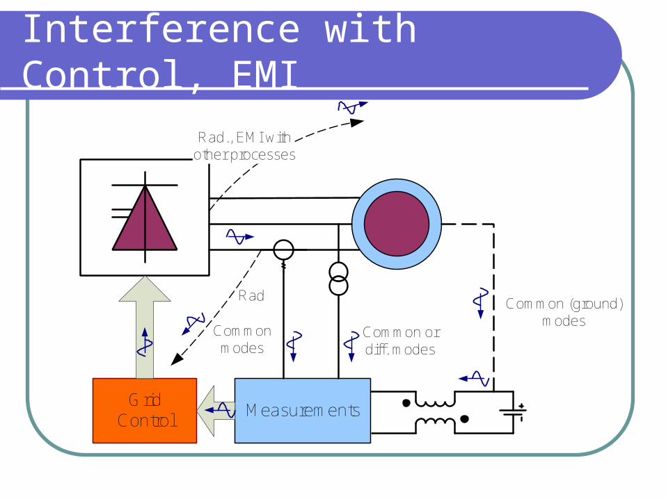
Interference with Control, EMI
Grid Control
Measurements
Rad Common (ground) modes
Common or diff. modes
Common modes
Rad., EMI with other processes

What Are Harmonics?
Technical DescriptionA high frequency sinusoidal current or voltage produced by certain non-linear and switching processes in the system during normal periodic operation (steady state);
The harmonic frequency is an integer multiple of the system operating frequency (fundamental).
The non-sinusoidal part in a periodic voltage or current is the harmonic ripple or harmonic distortion—comprised of harmonic frequencies.
Mathematical Definition Sine and cosine functions of time with frequencies that are integer
multiples of a fundamental frequency Harmonic sine and cosine functions sum up to a periodic (non-
sinusoidal) function Terms of the Fourier series expansion of a periodic function;
0 0.5 1 1.5
-100
-50
0
50
100
Time
% V
olts
Distortion of an AC Voltage
Specified
ActualDistortion
0 0.5 1 1.5
-20
0
20
40
60
80
100
DC Current Ripple
Time
% C
urre
nt
Specified Actual Ripple
0 0.5 1 1.5
-1
-0.5
0
0.5
1
AC Input from an Inverter
Actual
Desired
0 0.5 1 1.50
0.5
1
DC Input from a Diode Rectifier
Time
Actual
Desired
0 0.5 1 1.5-1
-0.5
0
0.5
1
Non-Harmonic Disturbance/Distortion
0 0.5 1 1.5
-1
0
1
Transient Response
Time
0 0.5 1 1.5
-1
-0.5
0
0.5
1
Non-periodic Steady State: Subharmonic Component
0 0.5 1 1.5
-1
-0.5
0
0.5
1
Non-periodic Steady State: Interharmonic Component
Time

Harmonic Analysis
What is it? Principles, properties and methods for expressing periodic
functions as sum of (harmonic) sine and cosine terms: Fourier Series Fourier Transform Discrete Fourier Transform
Where is it used? Obtain the response of a system to arbitrary periodic inputs;
quantify/assess harmonic effects at each frequency
Framework for describing the quality of the system input and output signals (spectrum)
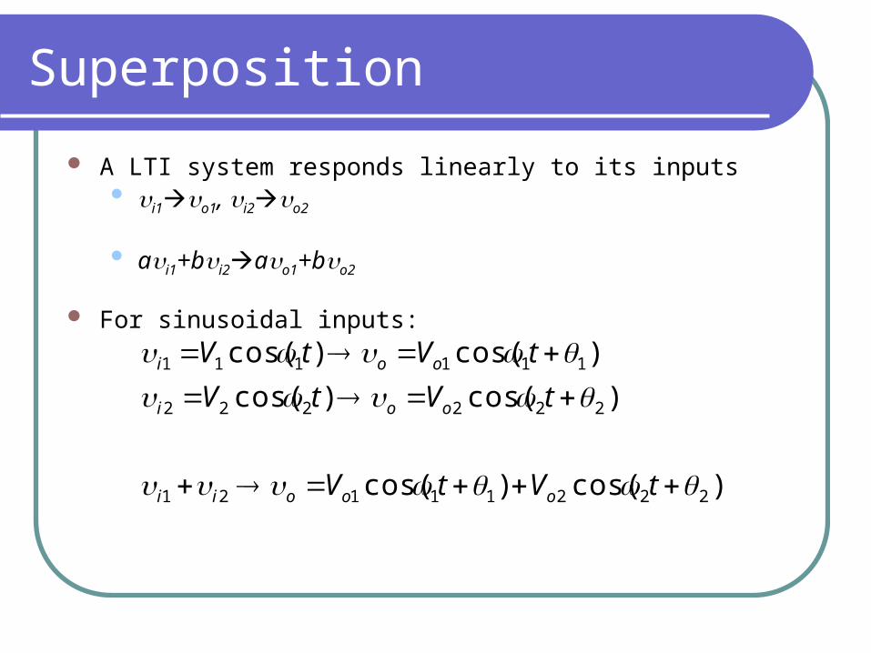
Superposition
A LTI system responds linearly to its inputs i1o1, i2o2
ai1+bi2ao1+bo2
For sinusoidal inputs:
)cos()cos(
)cos()cos(
)cos()cos(
22211121
222222
111111
tVtV
tVtV
tVtV
oooii
ooi
ooi

Application preview: DC Drive
is
Vts ),602sin(2402
E=150 VRa=1 WLa=5 mH
io
+
vo
-
Find the armature current io(t) below

DC Voltage Approximation
0 0.005 0.01 0.015 0.02 0.025
-200
0
200
Input Voltage
v s, V
0 0.005 0.01 0.015 0.02 0.0250
100
200
300
Output Voltage
v o, V
Time, s
Vttto )]3602cos(3.12)2402cos(8.28)1202cos(1.144[1.216
is
io
+
vo
-

Source Superposition
+
-
+
-
+
-
VV dco 1.216,
Vto )1202cos(1.1442,
Vto )2402cos(8.284,
Vto )3602cos(3.126,
Ra=1 W
E=150 V
La= 0.005 H
io
VV dco 1.216, Ra=1 W
E=150 V
AR
EVI
a
dcodco 1.66,
,
Vttto )]3602cos(3.12)2402cos(8.28)1202cos(1.144[1.216

Output Response
0 0.005 0.01 0.015 0.02 0.0250
100
200
300
Output Voltagev o,
V
0 0.005 0.01 0.015 0.02 0.0250
50
100
Output Current
i o, A
Time, s
Atttio )853602cos(08.1)4.822402cos(78.3)751202cos(9.361.66

Procedure to obtain response
Step 1: Obtain the harmonic composition of the input (Fourier Analysis)
Step 2: Obtain the system output at each input frequency (equivalent circuit, T.F. frequency response)
Step 3: Sum the outputs from Step 2.
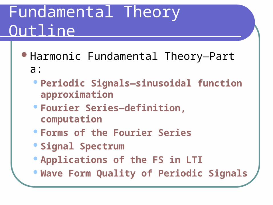
Fundamental Theory Outline
Harmonic Fundamental Theory—Part a:Periodic Signals—sinusoidal function
approximationFourier Series—definition, computationForms of the Fourier SeriesSignal SpectrumApplications of the FS in LTIWave Form Quality of Periodic Signals

Measures Describing the Magnitude of a Signal
Amplitude and Peak Value
Average Value or dc Offset
Root Mean Square Value (RMS) or Power

Amplitude and Peak Value
Peak of a Symmetric Oscillation
y
t
A
y
t
A
-A-A
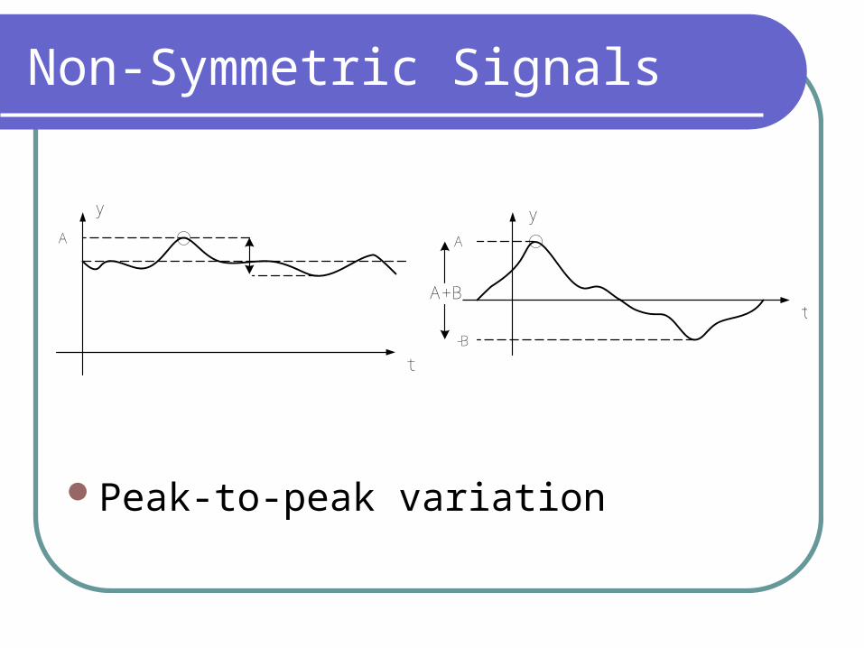
Non-Symmetric Signals
Peak-to-peak variation
y
t
A
y
t
A
-B
A+B

Average Value
Signal=(constant part) + (oscillating terms)
y
t
Yav
T
T
av dttyT
Y0
)(1

Examples
y
t
A
Yav=0
y
tT
Yav
kAYav
kT
A
y
t
Yav
-B
A
2
BAYav
y
t
A
A2

AC Signals
Zero Average Value
y
t
A
y
t
A
y
t

DC and Unidirectional Signals
y
t
Dc offset
y
t
Dc offset
y
t
y
t
A
A2

Root Mean Square Value (RMS)
T
rms dtyT
Y0
21For periodic signals, time window equals one period
y
tT
y2
tT
Yrms
T
rms dtyT
Y0
21

Remarks on RMS
RMS is a measure of the overall magnitude of the signal (also referred to as norm or power of the signal).
The rms of current and voltage is directly related to power.
Electric equipment rating and size is given in voltage and current rms values. IVS
R
VIRP
dtT
VdtiT
I
R
TT
22
0
2
0
2 1,
1

Examples of Signal RMS
y
t
A
y
tT
Yav AkYav
kT
A
Yrms kA
y
t
A
2
A
t
y120º
3
2A
A

Effect of DC Offset
New RMS=
SQRT [ (RMS of Unshifted)2+(DC offset)2]
y
t
y
t
d
2
2
2d
A
d
22 dA

Examples of Signals with equal RMS
y
t
A
2
A
y
t
y
t
A
2
A
2
A
t
y
3
2A
A

RMS and Amplitude
Amplitude: Local effects in time; Device insulation, voltage withstand break down, hot spots
RMS: Sustained effects in time; Heat dissipation, power output
y
t
A
y
t
y
t
2
A

Harmonic Analysis: Problem Statement
Approximate the square pulse function by a sinusoidal function in the interval [–T/2 , T/2]
f(t)
T/2 T-T -T/2 3T/2
11
-1
f(t)
T/2 T-T -T/2 3T/2
11
-1
)2
sin( tT
B
f(t)
T/2 T-T -T/2 3T/2
11
-1
)2
cos( tT
A

General Problem
Find a cosine function of period T that best fits a given function f(t) in the interval [0,T]
Assumptions:f(t) is periodic of period T
)()(
2
)cos()(
tFtfT
tAtF

Approximation Error
Error:
)cos()()()()( tAtftFtfte
f(t)
T/2-T/2
1
-1
A
e(t)
T/2-T/2
1
-1
Method:Find value of A that gives the Least Mean Square Error
Objective:Minimize the error e(t)

Define the average square error as
:
E is a quadratic function of A. The optimum choice of A is the one minimizing E.
T
dtteT
E
0
2)(1
TT
TT
dttfT
dtttfT
AA
E
dtttAftAtfT
dttAtfT
E
0
2
0
2
0
222
0
2
)(1
)cos()(2
2
)cos()(2)cos()(1
)cos()(1
Procedure

Optimum Value of A
dtttfT
AdA
dET
opt 0
)cos()(2
0
.)cos()(2
0
T
dtttfT
AdA
dE
Set dE/dA equal to zero
Find dE/dA:
TT
dttfT
dtttfT
AA
E
0
2
0
2
)(1
)cos()(2
2

EXAMPLE: SQUARE PULSE
-1.5 -1 -0.5 0 0.5 1 1.5
-1
0
1
-1.5 -1 -0.5 0 0.5 1 1.5
-1
0
1
-1.5 -1 -0.5 0 0.5 1 1.5
-1
0
1
Error-1.5 -1 -0.5 0 0.5 1 1.5
-1
0
1
-1.5 -1 -0.5 0 0.5 1 1.5
-1
0
1
Error
-1.5 -1 -0.5 0 0.5 1 1.5
-1
0
1
-1.5 -1 -0.5 0 0.5 1 1.5
-1
0
1
Error
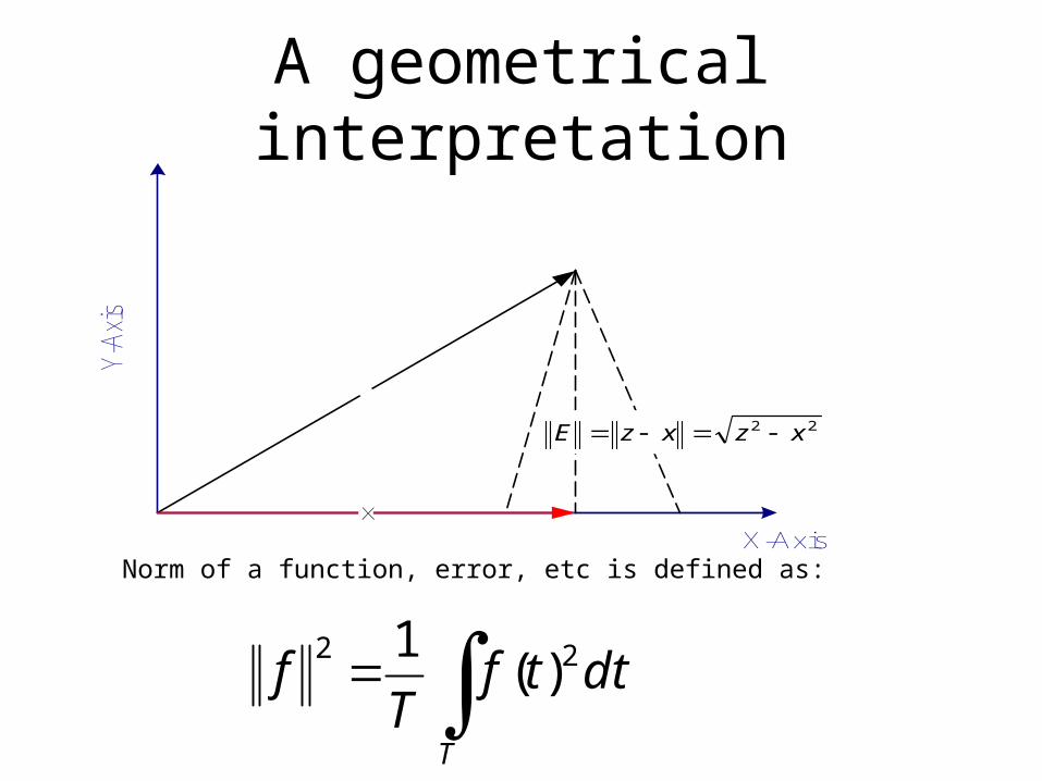
A geometrical interpretationY-
Axis
X-Axisx
22 xzxzE
T
dttfT
f 22)(
1
Norm of a function, error, etc is defined as:

Shifted Pulse
f(t-T/4)
T/2
1
-1
B
T
f(t-b)
T/2
1
-1
B
T
A
dttT
tfT
B
tBT
tf
T
0
)sin()4
(2
)sin()4
(
dttbtfT
B
dttbtfT
A
tBtAbtf
T
T
0
0
)sin()(2
)cos()(2
)sin()cos()(

A 2cos
(2t)
A3c
os(3
t)A1cos(t)f(t)
Average Square Error :
dttNBtNAtBtAtfT
E
T
NN
2
0
11 )sin()cos(sincos)(1
Approximation with many harmonic terms

Harmonic Basis
The terms ,1,0),sin(),cos( ntnBtnA nn From an orthogonal basis
Orthogonality property:
0)sin()cos(1
,2
1
,0
)sin()sin(1
)cos()cos(1
0
0 0
T
T T
dttktmT
mk
mk
dttktmT
dttktmT

Optimum coefficients
The property of orthogonality eliminates the cross harmonic product terms from the Sq. error
For each n, set
TTT
T
T
NN
dtfT
dttfT
BdttfT
ABA
dttBtAtBftAffT
dttNBtNAtBtAtfT
E
211
21
21
221
22111
2
2
0
11
1sin
2cos
2
2
1
2
1
sincossin2cos21
)sin()cos(sincos)(1
0
iA
E
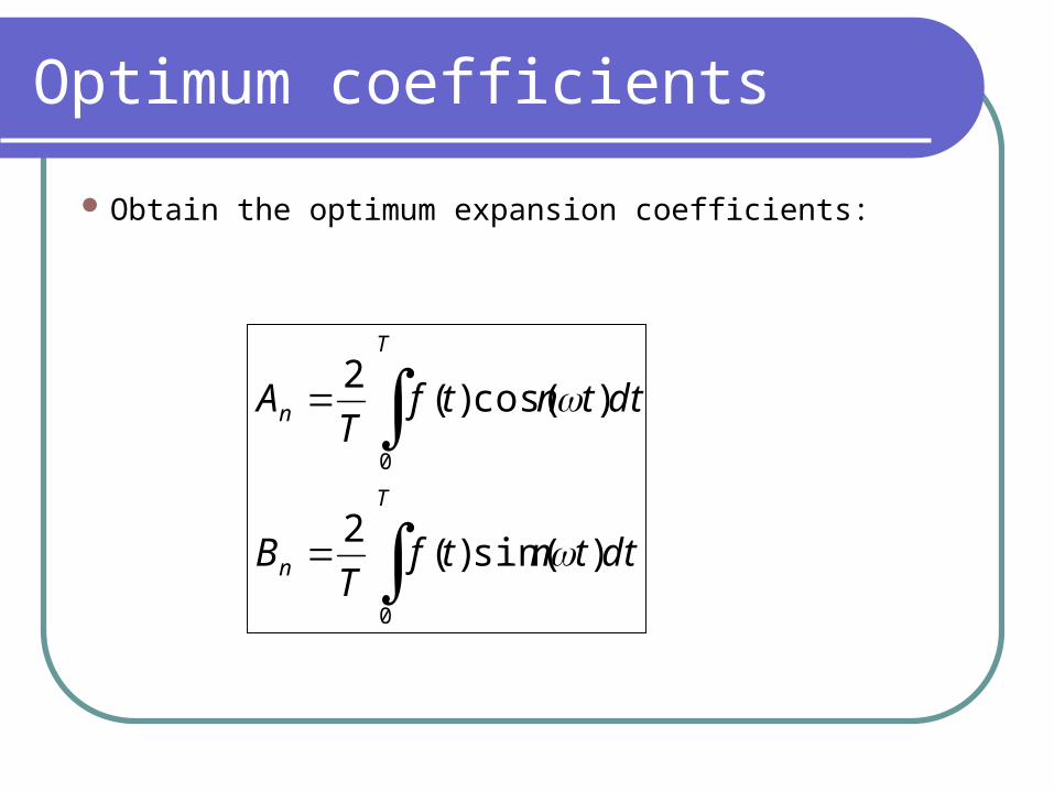
Optimum coefficients
Obtain the optimum expansion coefficients:
T
n
T
n
dttntfT
B
dttntfT
A
0
0
)sin()(2
)cos()(2

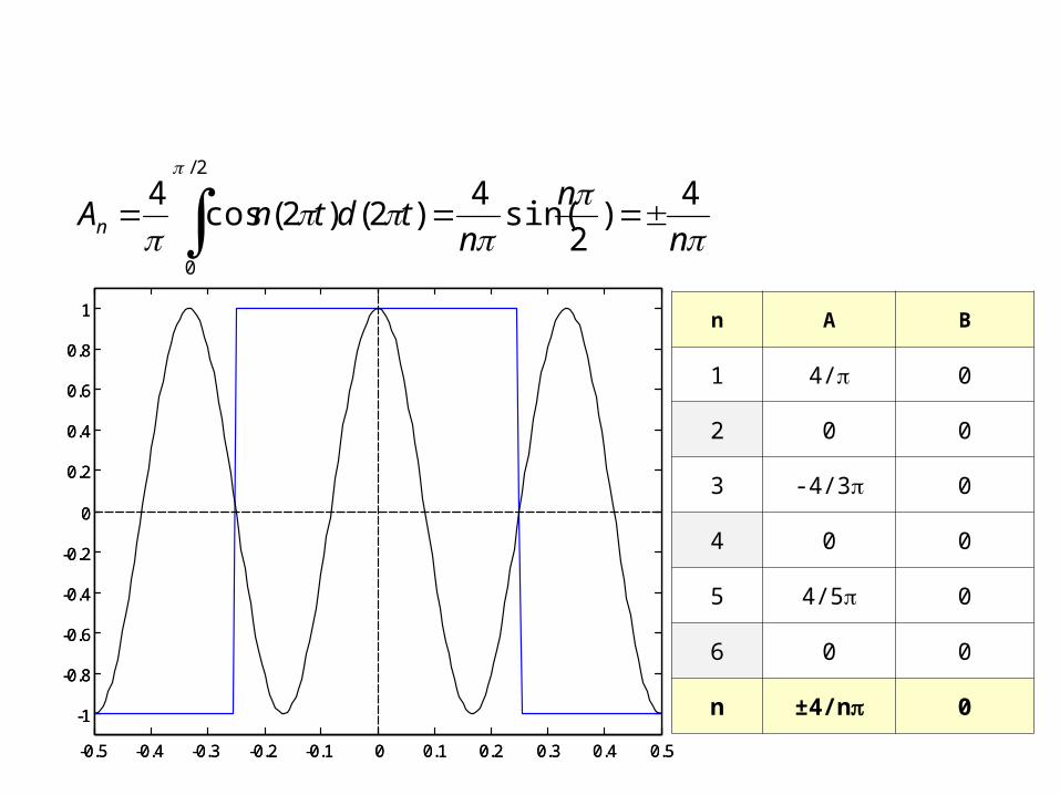
Example—Square Wave Pulse
-0.5 -0.4 -0.3 -0.2 -0.1 0 0.1 0.2 0.3 0.4 0.5
-1
-0.8
-0.6
-0.4
-0.2
0
0.2
0.4
0.6
0.8
1

-0.5 -0.4 -0.3 -0.2 -0.1 0 0.1 0.2 0.3 0.4 0.5
-1
-0.8
-0.6
-0.4
-0.2
0
0.2
0.4
0.6
0.8
1
4)2()2cos(
4(.)
2
)2()2cos()(1
)2cos()(2
2/
00
2/
2/
1
tdt
tdttfdtttfT
A
T
T

-0.5 -0.4 -0.3 -0.2 -0.1 0 0.1 0.2 0.3 0.4 0.5
-1
-0.8
-0.6
-0.4
-0.2
0
0.2
0.4
0.6
0.8
1
0)2()2sin()(2
)2()2sin()(1
0
1
tdttftdttfB

-0.5 -0.4 -0.3 -0.2 -0.1 0 0.1 0.2 0.3 0.4 0.5
-1
-0.8
-0.6
-0.4
-0.2
0
0.2
0.4
0.6
0.8
1
022 BA

-0.5 -0.4 -0.3 -0.2 -0.1 0 0.1 0.2 0.3 0.4 0.5
-1
-0.8
-0.6
-0.4
-0.2
0
0.2
0.4
0.6
0.8
1
3
4sin
3
4)2()2(3cos
42
3
2/
0
3 tdtA
-0.5 -0.4 -0.3 -0.2 -0.1 0 0.1 0.2 0.3 0.4 0.5
-1
-0.8
-0.6
-0.4
-0.2
0
0.2
0.4
0.6
0.8
1
-0.5 -0.4 -0.3 -0.2 -0.1 0 0.1 0.2 0.3 0.4 0.5
-1
-0.8
-0.6
-0.4
-0.2
0
0.2
0.4
0.6
0.8
1
n
n
ntdtnAn
4)
2sin(
4)2()2(cos
42/
0
n A B
1 4/ 0
2 0 0
3 -4/3 0
4 0 0
5 4/5 0
6 0 0
n ±4/n 0
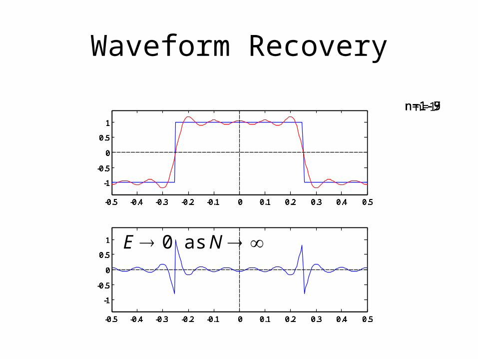
Waveform Recovery
-0.5 -0.4 -0.3 -0.2 -0.1 0 0.1 0.2 0.3 0.4 0.5
-1
-0.5
0
0.5
1
-0.5 -0.4 -0.3 -0.2 -0.1 0 0.1 0.2 0.3 0.4 0.5
-1
-0.5
0
0.5
1
-0.5 -0.4 -0.3 -0.2 -0.1 0 0.1 0.2 0.3 0.4 0.5
-1
-0.5
0
0.5
1
-0.5 -0.4 -0.3 -0.2 -0.1 0 0.1 0.2 0.3 0.4 0.5
-1
-0.5
0
0.5
1
-0.5 -0.4 -0.3 -0.2 -0.1 0 0.1 0.2 0.3 0.4 0.5
-1
-0.5
0
0.5
1
-0.5 -0.4 -0.3 -0.2 -0.1 0 0.1 0.2 0.3 0.4 0.5
-1
-0.5
0
0.5
1
-0.5 -0.4 -0.3 -0.2 -0.1 0 0.1 0.2 0.3 0.4 0.5
-1
-0.5
0
0.5
1
-0.5 -0.4 -0.3 -0.2 -0.1 0 0.1 0.2 0.3 0.4 0.5
-1
-0.5
0
0.5
1
-0.5 -0.4 -0.3 -0.2 -0.1 0 0.1 0.2 0.3 0.4 0.5
-1
-0.5
0
0.5
1
-0.5 -0.4 -0.3 -0.2 -0.1 0 0.1 0.2 0.3 0.4 0.5
-1
-0.5
0
0.5
1
n=1n=1-3n=1-5n=1-7n=1-9
NE as 0

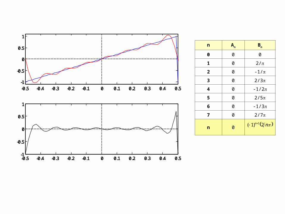
Example: Sawtooth
-2 -1.5 -1 -0.5 0 0.5 1 1.5 2-1
-0.8
-0.6
-0.4
-0.2
0
0.2
0.4
0.6
0.8
1

-0.5 -0.4 -0.3 -0.2 -0.1 0 0.1 0.2 0.3 0.4 0.5-1
-0.5
0
0.5
1
-0.5 -0.4 -0.3 -0.2 -0.1 0 0.1 0.2 0.3 0.4 0.5-1
-0.5
0
0.5
1
ndndt
Tdtntt
TB n
TT
T
n
2)1()()sin(
2)(
4)2sin(2
2 1
0
2/
0
2/
2/
Odd Symmetry
-0.5 -0.4 -0.3 -0.2 -0.1 0 0.1 0.2 0.3 0.4 0.5-1
-0.5
0
0.5
1
-0.5 -0.4 -0.3 -0.2 -0.1 0 0.1 0.2 0.3 0.4 0.5-1
-0.5
0
0.5
1
-0.5 -0.4 -0.3 -0.2 -0.1 0 0.1 0.2 0.3 0.4 0.5-1
-0.5
0
0.5
1
-0.5 -0.4 -0.3 -0.2 -0.1 0 0.1 0.2 0.3 0.4 0.5-1
-0.5
0
0.5
1
-0.5 -0.4 -0.3 -0.2 -0.1 0 0.1 0.2 0.3 0.4 0.5-1
-0.5
0
0.5
1
-0.5 -0.4 -0.3 -0.2 -0.1 0 0.1 0.2 0.3 0.4 0.5-1
-0.5
0
0.5
1
-0.5 -0.4 -0.3 -0.2 -0.1 0 0.1 0.2 0.3 0.4 0.5-1
-0.5
0
0.5
1
-0.5 -0.4 -0.3 -0.2 -0.1 0 0.1 0.2 0.3 0.4 0.5-1
-0.5
0
0.5
1
-0.5 -0.4 -0.3 -0.2 -0.1 0 0.1 0.2 0.3 0.4 0.5-1
-0.5
0
0.5
1
-0.5 -0.4 -0.3 -0.2 -0.1 0 0.1 0.2 0.3 0.4 0.5-1
-0.5
0
0.5
1
-0.5 -0.4 -0.3 -0.2 -0.1 0 0.1 0.2 0.3 0.4 0.5-1
-0.5
0
0.5
1
-0.5 -0.4 -0.3 -0.2 -0.1 0 0.1 0.2 0.3 0.4 0.5-1
-0.5
0
0.5
1
n An Bn
0 0 0
1 0 2/
2 0 -1/
3 0 2/3
4 0 -1/2
5 0 2/5
6 0 -1/3
7 0 2/7
n 0 nn 2)1( 1

Periodic Approximation
-2 -1.5 -1 -0.5 0 0.5 1 1.5 2
-1
-0.8
-0.6
-0.4
-0.2
0
0.2
0.4
0.6
0.8
1

Approximation of the Rectified sine
vo(t)
t
v(t)
t
Vm
TT/2
Vm
T
tVtv m
2
)sin()(
d=T/2
A periodic signal= (constant part)+(oscillating part)

Average Value
vo(t)
tTT/2
Vm
d=T/2
m
t
tmm
T
m
d
m
VtV
tdtV
dttVT
dttVd
A
2)cos()sin(
)sin(2
)sin(1
00
2/
00
0

Harmonic Terms
vo(t)
tTT/2
Vm
d=T/2
)12)(12(
4)12sin()12sin(
)2cos()sin(4
)2
cos()sin(2
0
2/
0
0
kk
Vtdtktk
V
dttktT
V
dttd
ktVd
A
mm
Tm
d
mk

Summary
vo(t)
t
v(t)
t
Vm
TT/2
Vm
T
tVtv m
2
)sin()(
,4,2
,2,1
)cos()1)(1(
142)(
)2(
)2cos()12)(12(
142)(
n
mmo
k
mmo
tnnn
VVtv
kn
tkkk
VVtv

Numerical Problem: DC Drive
is
Vts ),602sin(2402
E=150 VRa=1 WLa=5 mH
io
+
vo
-
0 0.005 0.01 0.015 0.02 0.025
-200
0
200
Input Voltage
v s, V
0 0.005 0.01 0.015 0.02 0.0250
100
200
300
Output Voltage
v o, V
Time, s

Input Harmonic Approximation
VVV mdco 1.2162
,
VVV mdco 1.2162
, 0 0.005 0.01 0.015 0.02 0.025
-200
0
200
Input Voltage
v s, V
0 0.005 0.01 0.015 0.02 0.0250
100
200
300
Output Voltage
v o, V
Time, s
Average or dc component)377sin(4.339)602sin(2402 tts
Harmonic Expansion
)602cos()1()1(
14
,4,2, tn
nn
VV
n
mdcoo
))3602cos(3.12)2402cos(8.28)1202cos(1.144(1.216 ttto
Truncated Approximation (n=2, 4, and 6)

Equivalent Circuit
is
Vts ),602sin(2402
E=150 VRa=1 WLa=5 mH
io
+
vo
-
))3602cos(3.12)2402cos(8.28)1202cos(1.144(1.216 ttto
+
-
+
-
+
-
VV dco 1.216,
Vto )1202cos(1.1442,
Vto )2402cos(8.284,
Vto )3602cos(3.126,
Ra=1 W
E=150 V
La= 0.005 H
io

Superimpose Sources: DC Source
+
-
+
-
+
-
VV dco 1.216,
Vto )1202cos(1.1442,
Vto )2402cos(8.284,
Vto )3602cos(3.126,
Ra=1 W
E=150 V
La= 0.005 H
io
VV dco 1.216, Ra=1 W
E=150 V
AR
EVI
a
dcodco 1.66,
,

Superposition: n=2, f=120 Hz
+
-
+
-
+
-
VV dco 1.216,
Vto )1202cos(1.1442,
Vto )2402cos(8.284,
Vto )3602cos(3.126,
Ra=1 W
E=150 V
La= 0.005 H
io
VVo 1.1442,Ra=1 W
AZ
VI
a
oo )75(9.3675
9.3
1.1442,2,
+
-
W77.3
)1202(
i
LiiX aa
W
759.377.31
)2(
i
iXRZ aaa
)751202cos(9.36)751202cos(9.362 ttio

Superposition: n=4, f=240 Hz
+
-
+
-
+
-
VV dco 1.216,
Vto )1202cos(1.1442,
Vto )2402cos(8.284,
Vto )3602cos(3.126,
Ra=1 W
E=150 V
La= 0.005 H
io
VVo 8.284,
Ra=1 W
AZ
VI
a
oo )4.82(78.34.82
61.7
8.284,4,
+
-
W54.7
)2402(
i
LiiX aa
W
4.8261.754.71
)4(
i
iXRZ aaa
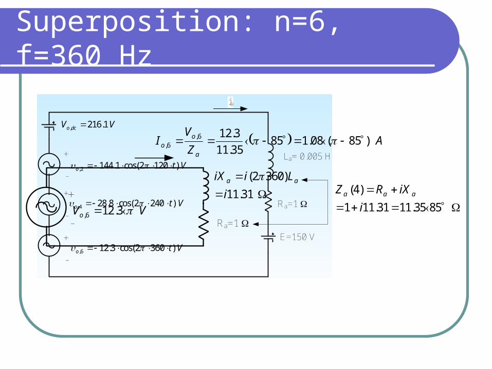
Superposition: n=6, f=360 Hz
+
-
+
-
+
-
VV dco 1.216,
Vto )1202cos(1.1442,
Vto )2402cos(8.284,
Vto )3602cos(3.126,
Ra=1 W
E=150 V
La= 0.005 H
io
VVo 3.126,Ra=1 W
AZ
VI
a
oo )85(08.185
35.11
3.126,6,
+
-
W
31.11
)3602(
i
LiiX aa
W
8535.1131.111
)4(
i
iXRZ aaa

Summary
Freq., Hz
Vo ampl, V Io ampl, A Za magn, W Power loss, W
0 (dc) 216.1 66.1 1 4,369.2
120 144.1 36.9 3.9 680.8
240 28.8 3.78 7.61 7.14
360 12.3 1.08 11.35 .583
RMS 240 71.1Total Power Loss
5,057.7
Output Power(66.1A)(150V)
9,915
2
9.361
22
222,
2
2,2,
AIR
IRP o
ao
ah W
22,, 1.661 AIRP dcoadco W

Output Time and Frequency Response
0 2 4 60
50
100
150
200
250Output Spectra
Voh
, V
and
I oh,
A
Harmonic Number
Voltage
Current
0 0.005 0.01 0.015 0.02 0.0250
100
200
300
Output Voltage
v o, V
0 0.005 0.01 0.015 0.02 0.0250
50
100
Output Current
i o, A
Time, s0 0.005 0.01 0.015 0.02 0.025
-300
-200
-100
0
100
200
300
Input Voltage and Current
v s, V
and
i s, A
Time, s
Atttio )853602cos(08.1)4.822402cos(78.3)751202cos(9.361.66 is
io
+
vo
-

Generalization: Fourier Series
The Fourier theorem states that a bounded periodic function f(t) with limited finite number of discontinuities can be described by an infinite series of sine and cosine terms of frequency that is the integer multiple of the fundamental frequency of f(t):
1
0 )sin()cos()( tnBtnAAtf nn
Where
T
dttfT
A
0
0 )(1
is the zero frequency or average value of f(t).
Waveform Symmetry
Half Wave SymmetryQuarter Wave Symmetry
OddEven
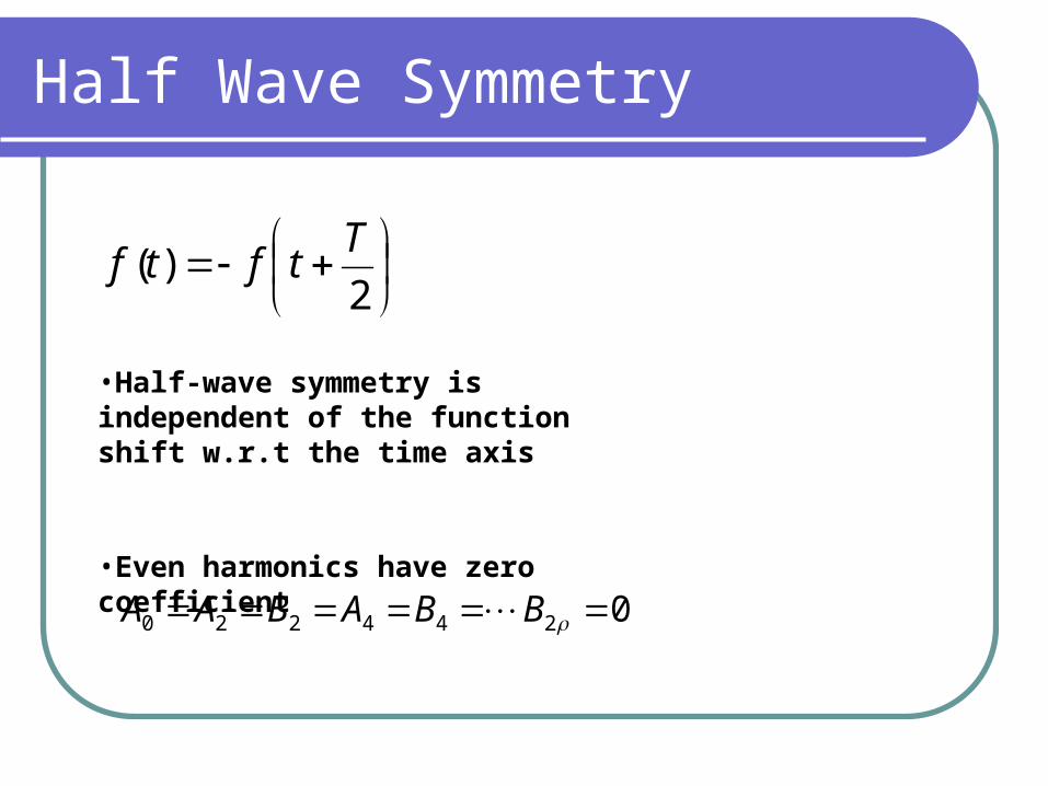
Half Wave Symmetry
2)(
Ttftf
0244220 BBABAA
•Half-wave symmetry is independent of the function shift w.r.t the time axis
•Even harmonics have zero coefficient

Square Wave
-2 -1.5 -1 -0.5 0 0.5 1 1.5 2
-1
-0.8
-0.6
-0.4
-0.2
0
0.2
0.4
0.6
0.8
1
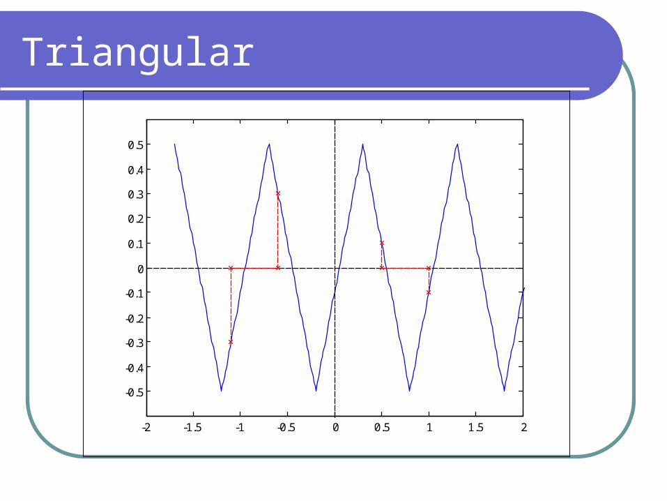
Triangular
-2 -1.5 -1 -0.5 0 0.5 1 1.5 2
-0.5
-0.4
-0.3
-0.2
-0.1
0
0.1
0.2
0.3
0.4
0.5

Saw Tooth—Counter Example
-2 -1.5 -1 -0.5 0 0.5 1 1.5 2
-1
-0.8
-0.6
-0.4
-0.2
0
0.2
0.4
0.6
0.8
1
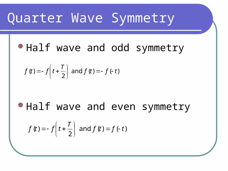
Quarter Wave Symmetry
Half wave and odd symmetry
Half wave and even symmetry
)()( and2
)( tftfT
tftf
)()( and 2
)( tftfT
tftf
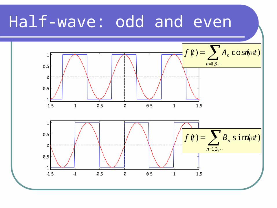
Half-wave: odd and even
-1.5 -1 -0.5 0 0.5 1 1.5-1
-0.5
0
0.5
1
-1.5 -1 -0.5 0 0.5 1 1.5-1
-0.5
0
0.5
1
,3,1
)cos()(n
n tnAtf
,3,1
)sin()(n
n tnBtf
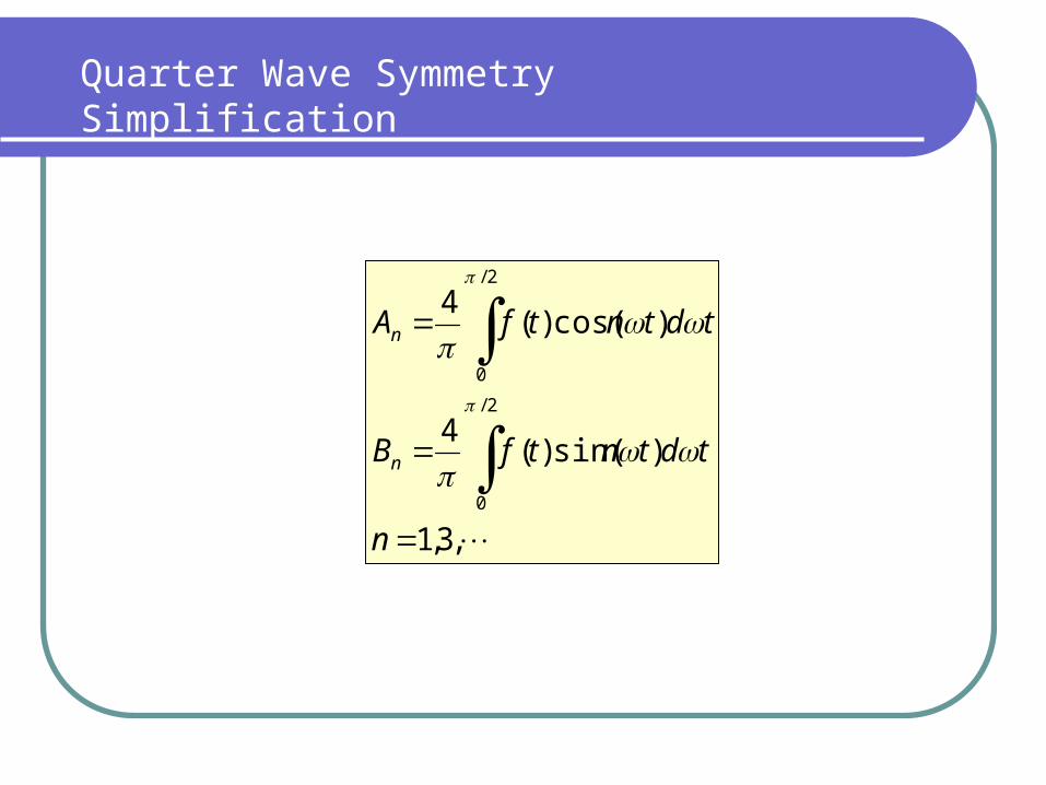
Quarter Wave Symmetry Simplification
,3,1
)sin()(4
)cos()(4
2/
0
2/
0
n
tdtntfB
tdtntfA
n
n

Forms of the Fourier Transform
Trigonometric
Combined Trigonometric
Exponential

n
nn
n
nnn
A
B
tnBAAtf
arctan
)cos()(,2,1
220
n
nnnnn A
BtnBAtnBtnA arctancos)sin()cos( 22
1
0 )sin()cos()(n
nn tnBtnAAtf
•Trigonometric form
•Combined Trigonometric

•Exponential
*
)sin()cos()(1
)(1
)(
nn
TT
tjnn
n
tjnn
CC
dttnjtntfT
dtetfT
C
eCtf
tjnn
tjnn
tjnjnntjnjnn
tnjtnjnnnnn
jj
eCeCeeBA
eeBA
eeBA
tnBAee
nn
nn
22
2)cos(
2cos
2222
)()(22
22
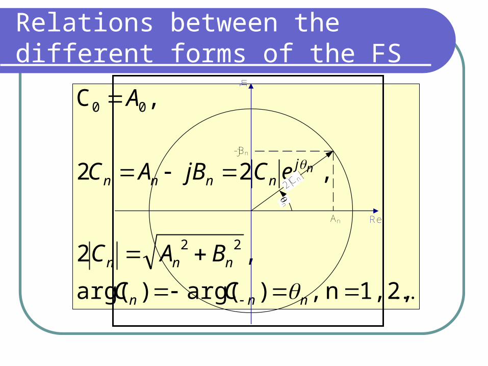
Relations between the different forms of the FS
1,2,n ,)arg()arg(
,2
, 22
,C
22
00
nnn
nnn
jnnnn
CC
BAC
eCjBAC
A
n
Re
Im
2|Cn|
n
An
-jBn

Series Type f(t)=
Trigonometric
,2,1
0 )sin()cos(n
nn tnBtnAA
,,ndttntfT
B
dttntfT
A
dttfT
A
n
T
n
T
21 ,)sin()(2
)cos()(2
)(1
0
Combined Trigonometric (Phasor form, Harmonic amplitude and phase)
n
nn
n
nnn A
BtnBAA arctan ,)cos(
,2,1
220
Exponential
T
tjnn
n
tjnn etf
TCeC )(
1 , ,
*
2221
21
21
00
,2,1 ,
nn
jnnnnn
CC
neBABjAC
AC
n
Summary of FS Formulas

Re
Im
2|Cn|
n
na
An
-jBn
Time Shift )()( atftf shifts
unchangedremain , 22nnn
ajnn
changesn
nchanges
n
BAC
eCC
an

Example: SQP -90° Shift
-1.5 -1 -0.5 0 0.5 1 1.5
-1
-0.8
-0.6
-0.4
-0.2
0
0.2
0.4
0.6
0.8
1
-1.5 -1 -0.5 0 0.5 1 1.5
-1
-0.8
-0.6
-0.4
-0.2
0
0.2
0.4
0.6
0.8
1
original shifted
n 2|Cn| n n
1 4/ 0
2 0 0 -
3 4/3
4 0 0 -
5 4/5 0
6 0 0 -
7 5/7
n 4/n (n-1)/2 -/2

Example: SQP -60° Shift
-1.5 -1 -0.5 0 0.5 1 1.5
-1
-0.8
-0.6
-0.4
-0.2
0
0.2
0.4
0.6
0.8
1
-1.5 -1 -0.5 0 0.5 1 1.5
-1
-0.8
-0.6
-0.4
-0.2
0
0.2
0.4
0.6
0.8
1
original shifted
n 2|Cn| n n
1 4/ 0
2 0 0 -
3 4/3
4 0 0 -
5 4/5 0
6 0 0 -
7 5/7
n 4/n (n-1)/2 (n-3)/6

SPECTRUM: SQ. Pulse (amplitude=1)
n4
1 2 3 4 5 6 7 8 9 10 11 12 13 14 150
0.5
1
1.5
Mag
nitu
de,
2|C
n|
1 2 3 4 5 6 7 8 9 10 11 12 13 14 15-4
-3
-2
-1
0
Harmonic Order
Har
mon
ic p
hase
ang
le,
rad
-20 -15 -10 -5 0 5 10 15 200
0.2
0.4
0.6
0.8
|Cn|
-20 -15 -10 -5 0 5 10 15 20-4
-2
0
2
4
arg(
Cn)
Freq.
n2

SPECTRUM: Sawtooth (amplitude=1)
n2
1 2 3 4 5 6 7 8 9 10 11 12 13 14 150
0.2
0.4
0.6
0.8
Mag
nitu
de,
2|C
n|
1 2 3 4 5 6 7 8 9 10 11 12 13 14 150
1
2
3
4
5
Harmonic Order
Har
mon
ic p
hase
ang
le,
rad

SPECTRUM: Triangular wave (amplitude=1)
28
n
1 2 3 4 5 6 7 8 9 10 11 12 13 14 150
0.2
0.4
0.6
0.8
1
Mag
nitu
de,
2|C
n|
1 2 3 4 5 6 7 8 9 10 11 12 13 14 15-1
-0.5
0
0.5
1
Harmonic Order
Har
mon
ic p
hase
ang
le,
rad

SPECTRUM: Rectified SINE (peak=1)
)1(
42 n
0 2 4 6 8 10 12 140
0.1
0.2
0.3
0.4
0.5
0.6
Harmonic Order
Mag
nitu
de: C
0 and
2|C
n|, n=
1,2.
.

Using FS to Find the Steady State Response of an LTI System
11 1
1
1
1
][
][][
1
1
1
1)(
jnRCjnnU
nUnH
ies:c frequencAt harmoni
jRCjU
UH
in
out
in
out
)1
arctan(][arg][arg][arg][arg
,)(1
][][][][
][1
1][][][
21
1
nnin
UnHnUnU
n
nUnUnHnU
nUjn
nUnHnU
inout
ininout
ininout
5kW
1mF
+
-
+
-
inout
=0.005 s
5kW
106/jn(2f1)
+
-
+
-
Uin[n] Uout[n]= ][)2(005.01
1
1
nUnfj in
Input periodic, fundamental freq.=f1=60 HzVoltage Division
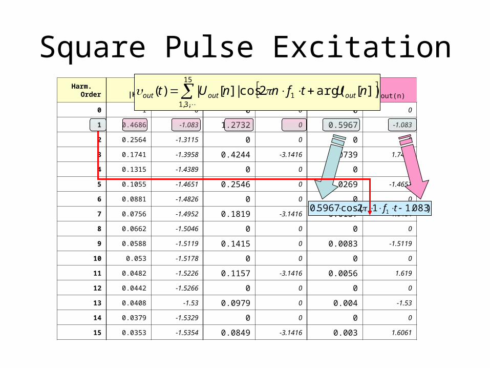
Square Pulse ExcitationHarm.
OrderCirc. TF
|H(n)|, <H(n)Inp.
|Uin(n)|, <Uin(n)
Out.|Uout(n)|, <Uout(n)
0 1 0 0 0 0 0
1 0.4686 -1.083 1.2732 0 0.5967 -1.083
2 0.2564 -1.3115 0 0 0 0
3 0.1741 -1.3958 0.4244 -3.1416 0.0739 1.7458
4 0.1315 -1.4389 0 0 0 0
5 0.1055 -1.4651 0.2546 0 0.0269 -1.4651
6 0.0881 -1.4826 0 0 0 0
7 0.0756 -1.4952 0.1819 -3.1416 0.0137 1.6464
8 0.0662 -1.5046 0 0 0 0
9 0.0588 -1.5119 0.1415 0 0.0083 -1.5119
10 0.053 -1.5178 0 0 0 0
11 0.0482 -1.5226 0.1157 -3.1416 0.0056 1.619
12 0.0442 -1.5266 0 0 0 0
13 0.0408 -1.53 0.0979 0 0.004 -1.53
14 0.0379 -1.5329 0 0 0 0
15 0.0353 -1.5354 0.0849 -3.1416 0.003 1.6061
)083.112cos(5967.0 1 tf
15
,3,11 ])[arg(2cos|][|)(
nUtfnnUt outoutout

SQUARE PULSE Excitation
0 5 10 150
0.5
1
input
output
-0.025 -0.02 -0.015 -0.01 -0.005 0 0.005 0.01 0.015 0.02 0.025-1
-0.5
0
0.5
1
time, s

Rectified SINE Wave
Harm. OrderCirc. TF
|H(n)|, <H(n)Inp.
|Uin(n)|, <Uin(n)
Out.|Uout(n)|, <Uout(n)
0 1 0 0.6366 0 0.6366 0
1 0.4686 -1.083 0 0 0 0
2 0.2564 -1.3115 0.0849 3.1416 0.0218 1.8301
3 0.1741 -1.3958 0 0 0 0
4 0.1315 -1.4389 0.0202 3.1416 0.0027 1.7027
5 0.1055 -1.4651 0 0 0 0
6 0.0881 -1.4826 0.0089 3.1416 0.0008 1.659
7 0.0756 -1.4952 0 0 0 0
8 0.0662 -1.5046 0.005 3.1416 0.0003 1.637
9 0.0588 -1.5119 0 0 0 0
10 0.053 -1.5178 0.0032 3.1416 0.0002 1.6238
11 0.0482 -1.5226 0 0 0 0
12 0.0442 -1.5266 0.0022 3.1416 0.0001 1.615
13 0.0408 -1.53 0 0 0 0
14 0.0379 -1.5329 0.0016 3.1416 0.0001 1.6087
15 0.0353 -1.5354 0 0 0 0

Rect. SINE wave
0 5 10 150
0.2
0.4
0.6
input
output
-0.025 -0.02 -0.015 -0.01 -0.005 0 0.005 0.01 0.015 0.02 0.0250
0.2
0.4
0.6
0.8
1
time, s

Total RMS of A Signal
2,1
0 )cos(2)(n
nn tnFAtf
nnnn CBAF 2222
T
rms dttfT
F 2)(1
Rewrite the FS as:
Nth harmonic rms (except for n=0)
Total rms of the wave form:

Total RMS and the FS Terms
T n
nn
T
rms dttnFAT
dttfT
F
2
2,1
022 )cos(2
1)(
1
2,1
220
2
n
nrms FAF
221
,3,2
221
2H
n
nrms FFFFF
For ac wave forms (A0=0) it is convenient to write:
Using the orthogonalitybetween the terms:
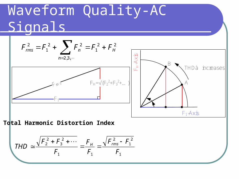
Waveform Quality-AC Signals
221
,3,2
221
2H
n
nrms FFFFF
1
21
2
11
23
22
F
FF
F
F
F
FFTHD rmsH
Total Harmonic Distortion Index
A
B
F1-Axis
FH-A
xis
THDà increases
F1
FH=√(F22+F3
2+…)Frms

Waveform Quality-DC SIgnals (A0≠0)
,4,2
2
0
2224
22
20
2
n
nac
dc
acdcrms
FF
AF
FFFFAF
dc
dcrms
dc
ac
F
FF
F
FRF
22
Ripple FactorFdc
Fac=√(F22+F4
2+…)Frms

Example: W.F.Q. of the circuit driven by a Sq.P.
Harm. OrderInp. Rms:|Uin(n)|/√2
Out. Rms:|Uout(n)|/√2
0 0 0
1 0.900288 0.421931
2 0 0
3 0.300096 0.052255
4 0 0
5 0.180029 0.019021
6 0 0
7 0.128623 0.009687
8 0 0
9 0.100056 0.005869
10 0 0
11 0.081812 0.00396
12 0 0
13 0.069226 0.002828
14 0 0
15 0.060033 0.002121
RMS1.00
(excact)0.4258
%THD48.43(exact)
13.6
4359.09.01 22
%43.48%1009.0
4359.0
√(0.42582 – 0.42192)=0.0575{
%6.13%1004219.0
0575.0

Example: WFQ of the circuit driven by a rect. sine
Harm. OrderInp. Rms:|Uin(n)|/√2
Out. Rms:|Uout(n)|/√2
0 0.6366=Uin(0) 0.6366=Uout(0)
1 0 0
2 0.060033 0.015415
3 0 0
4 0.014284 0.001909
5 0 0
6 0.006293 0.000566
7 0 0
8 0.003536 0.000212
9 0 0
10 0.002263 0.000141
11 0 0
12 0.001556 7.07E-05
13 0 0
14 0.001131 7.07E-05
15 0 0
RMS0.707(exact)
0.6368
%RF48.35(exact)
2.5%35.48%100
6366.0
3078.0
3078.06366.0707.0 22 01596.06366.06368.0 22
%5.2%1006366.0
01596.0