tutorial: labview mathscript

UniversityCollegeofSoutheastNorway

http://home.hit.no/~hansha

LabVIEWMathScriptHans-PetterHalvorsen,2016.10.31

ii

PrefaceThisdocumentexplainsthebasicconceptsofusingLabVIEWMathScript.

FormoreinformationaboutLabVIEW,visitmyBlog:http://home.hit.no/~hansha/

WhatisLabVIEW?

LabVIEW(shortforLaboratoryVirtualInstrumentationEngineeringWorkbench)isaplatformanddevelopmentenvironmentforavisualprogramminglanguagefromNationalInstruments.Thegraphicallanguageisnamed"G".

WhatisMATLAB?

MATLABisatoolfortechnicalcomputing,computationandvisualizationinanintegratedenvironment.MATLABisanabbreviationforMATrixLABoratory,soitiswellsuitedformatrixmanipulationandproblemsolvingrelatedtoLinearAlgebra.

MATLABofferslotsofadditionalToolboxesfordifferentareassuchasControlDesign,ImageProcessing,DigitalSignalProcessing,etc.

WhatisMathScript?

MathScriptisahigh-level,text-basedprogramminglanguage.MathScriptincludesmorethan800built-infunctionsandthesyntaxissimilartoMATLAB.Youmayalsocreatecustom-madem-filelikeyoudoinMATLAB.

MathScriptisanadd-onmoduletoLabVIEWbutyoudon’tneedtoknowLabVIEWprogramminginordertouseMathScript.IfyouwanttointegrateMathScriptfunctions(built-inorcustom-madem-files)aspartofaLabVIEWapplicationandcombinegraphicalandtextualprogramming,youcanworkwiththeMathScriptNode.

InadditiontotheMathScriptbuilt-infunctions,differentadd-onmodulesandtoolkitsinstallsadditionalfunctions.TheLabVIEWControlDesignandSimulationModuleandLabVIEWDigitalFilterDesignToolkitinstalllotsofadditionalfunctions.

YoucanmoreinformationaboutMathScripthere:http://www.ni.com/labview/mathscript.htm

HowdoyoustartusingMathScript?

YouneedtoinstallLabVIEWandtheLabVIEWMathScriptRTModule.Whennecessarysoftwareisinstalled,startMathScriptbyopenLabVIEW:

IntheGettingStartedwindow,selectTools->MathScriptWindow...:

iv

TableofContentsPreface......................................................................................................................................ii

TableofContents.....................................................................................................................iv

1 IntroductiontoLabVIEW...................................................................................................1

1.1 Dataflowprogramming...............................................................................................1

1.2 Graphicalprogramming..............................................................................................1

1.3 Benefits.......................................................................................................................2

1.4 LabVIEWMathScriptRTModule................................................................................2

2 LabVIEWMathScriptRTModule.......................................................................................4

3 LabVIEWMathScript.........................................................................................................5

3.1 Introduction................................................................................................................5

3.2 Help.............................................................................................................................7

3.3 Examples.....................................................................................................................7

3.4 Usefulcommands.....................................................................................................10

CallingfunctionsInMathScript...........................................................................................10

User-DefinedFunctionsInMathScript................................................................................11

Scripts..................................................................................................................................12

3.5 FlowControl.............................................................................................................14

3.5.1 If-elseStatement...............................................................................................14

3.5.2 SwitchandCaseStatement...............................................................................14

3.5.3 Forloop.............................................................................................................15

3.5.4 Whileloop.........................................................................................................15

3.6 Plotting.....................................................................................................................16

v TableofContents

Tutorial:LabVIEWMathScript

4 LinearAlgebraExamples.................................................................................................18

4.1 Vectors......................................................................................................................18

4.2 Matrices....................................................................................................................19

4.2.1 Transpose..........................................................................................................19

4.2.2 Diagonal.............................................................................................................20

4.2.3 Triangular..........................................................................................................21

4.2.4 MatrixMultiplication.........................................................................................21

4.2.5 MatrixAddition.................................................................................................22

4.2.6 Determinant......................................................................................................22

4.2.7 InverseMatrices................................................................................................23

4.3 Eigenvalues...............................................................................................................24

4.4 SolvingLinearEquations...........................................................................................25

4.5 LUfactorization.........................................................................................................26

4.6 TheSingularValueDecomposition(SVD).................................................................27

4.7 Commands................................................................................................................28

5 ControlDesignandSimulation........................................................................................29

5.1 State-spacemodelsandTransferfunctions.............................................................29

5.1.1 PID.....................................................................................................................30

5.1.2 State-spacemodel.............................................................................................31

5.1.3 Transferfunction...............................................................................................32

5.1.4 FirstOrderSystems...........................................................................................33

5.1.5 SecondOrderSystems.......................................................................................34

5.1.6 Padé-approximation..........................................................................................36

5.2 FrequencyResponseAnalysis...................................................................................37

5.2.1 BodeDiagram....................................................................................................38

TimeResponse....................................................................................................................41

vi TableofContents


6 MathScriptNode.............................................................................................................43

6.1 TransferringMathScriptNodesbetweenComputers...............................................45

6.2 Examples...................................................................................................................45

6.3 Exercises...................................................................................................................49

7 MATLABScript.................................................................................................................50

AppendixA–MathScriptFunctionsforControlandSimulation............................................51

1

1 IntroductiontoLabVIEWLabVIEW(shortforLaboratoryVirtualInstrumentationEngineeringWorkbench)isaplatformanddevelopmentenvironmentforavisualprogramminglanguagefromNationalInstruments.Thegraphicallanguageisnamed"G".OriginallyreleasedfortheAppleMacintoshin1986,LabVIEWiscommonlyusedfordataacquisition,instrumentcontrol,andindustrialautomationonavarietyofplatformsincludingMicrosoftWindows,variousflavorsofUNIX,Linux,andMacOSX.ThelatestversionofLabVIEWisversionLabVIEW2009,releasedinAugust2009.VisitNationalInstrumentsatwww.ni.com.

Thecodefileshavetheextension“.vi”,whichisanabbreviationfor“VirtualInstrument”.LabVIEWofferslotsofadditionalAdd-OnsandToolkits.

1.1 DataflowprogrammingTheprogramminglanguageusedinLabVIEW,alsoreferredtoasG,isadataflowprogramminglanguage.Executionisdeterminedbythestructureofagraphicalblockdiagram(theLV-sourcecode)onwhichtheprogrammerconnectsdifferentfunction-nodesbydrawingwires.Thesewirespropagatevariablesandanynodecanexecuteassoonasallitsinputdatabecomeavailable.Sincethismightbethecaseformultiplenodessimultaneously,Gisinherentlycapableofparallelexecution.Multi-processingandmulti-threadinghardwareisautomaticallyexploitedbythebuilt-inscheduler,whichmultiplexesmultipleOSthreadsoverthenodesreadyforexecution.

1.2 GraphicalprogrammingLabVIEWtiesthecreationofuserinterfaces(calledfrontpanels)intothedevelopmentcycle.LabVIEWprograms/subroutinesarecalledvirtualinstruments(VIs).EachVIhasthreecomponents:ablockdiagram,afrontpanel,andaconnectorpanel.ThelastisusedtorepresenttheVIintheblockdiagramsofother,callingVIs.Controlsandindicatorsonthefrontpanelallowanoperatortoinputdataintoorextractdatafromarunningvirtualinstrument.However,thefrontpanelcanalsoserveasaprogrammaticinterface.Thusavirtualinstrumentcaneitherberunasaprogram,withthefrontpanelservingasauserinterface,or,whendroppedasanodeontotheblockdiagram,thefrontpaneldefinesthe

2 IntroductiontoLabVIEW


inputsandoutputsforthegivennodethroughtheconnectorpane.ThisimplieseachVIcanbeeasilytestedbeforebeingembeddedasasubroutineintoalargerprogram.

Thegraphicalapproachalsoallowsnon-programmerstobuildprogramssimplybydragginganddroppingvirtualrepresentationsoflabequipmentwithwhichtheyarealreadyfamiliar.TheLabVIEWprogrammingenvironment,withtheincludedexamplesandthedocumentation,makesitsimpletocreatesmallapplications.Thisisabenefitononeside,butthereisalsoacertaindangerofunderestimatingtheexpertiseneededforgoodquality"G"programming.Forcomplexalgorithmsorlarge-scalecode,itisimportantthattheprogrammerpossessanextensiveknowledgeofthespecialLabVIEWsyntaxandthetopologyofitsmemorymanagement.ThemostadvancedLabVIEWdevelopmentsystemsofferthepossibilityofbuildingstand-aloneapplications.Furthermore,itispossibletocreatedistributedapplications,whichcommunicatebyaclient/serverscheme,andarethereforeeasiertoimplementduetotheinherentlyparallelnatureofG-code.

1.3 BenefitsOnebenefitofLabVIEWoverotherdevelopmentenvironmentsistheextensivesupportforaccessinginstrumentationhardware.Driversandabstractionlayersformanydifferenttypesofinstrumentsandbusesareincludedorareavailableforinclusion.Thesepresentthemselvesasgraphicalnodes.Theabstractionlayersofferstandardsoftwareinterfacestocommunicatewithhardwaredevices.Theprovideddriverinterfacessaveprogramdevelopmenttime.ThesalespitchofNationalInstrumentsis,therefore,thatevenpeoplewithlimitedcodingexperiencecanwriteprogramsanddeploytestsolutionsinareducedtimeframewhencomparedtomoreconventionalorcompetingsystems.Anewhardwaredrivertopology(DAQmxBase),whichconsistsmainlyofG-codedcomponentswithonlyafewregistercallsthroughNIMeasurementHardwareDDK(DriverDevelopmentKit)functions,providesplatformindependenthardwareaccesstonumerousdataacquisitionandinstrumentationdevices.TheDAQmxBasedriverisavailableforLabVIEWonWindows,MacOSXandLinuxplatforms.

FormoreinformationaboutLabVIEW,visitmyBlog:http://home.hit.no/~hansha/

1.4 LabVIEWMathScriptRTModuleTheLabVIEWMathScriptRTModuleisanadd-onmoduletoLabVIEW.WithLabVIEWMathScriptRTModuleyoucan:

3 IntroductiontoLabVIEW


• Deployyourcustom.mfilestoNIreal-timehardware• ReusemanyofyourscriptscreatedwithTheMathWorks,Inc.MATLAB®softwareand

others• Developyour.mfileswithaninteractivecommand-lineinterface• EmbedyourscriptsintoyourLabVIEWapplicationsusingtheMathScriptNode

4

2 LabVIEWMathScriptRTModule

YoucanworkwithLabVIEWMathScriptthrougheitheroftwointerfaces:the“LabVIEWMathScriptInteractiveWindow”orthe“MathScriptNode”.

YoucanworkwithLabVIEWMathScriptRTModulethroughbothinteractiveandprogrammaticinterfaces.Foraninteractiveinterfaceinwhichyoucanload,save,design,andexecuteyour.mfilescripts,youcanworkwiththe“MathScriptInteractiveWindow”.Todeployyour.mfilescriptsaspartofaLabVIEWapplicationandcombinegraphicalandtextualprogramming,youcanworkwiththe“MathScriptNode”.

TheLabVIEWMathScriptRTModulecomplementstraditionalLabVIEWgraphicalprogrammingforsuchtasksasalgorithmdevelopment,signalprocessing,andanalysis.TheLabVIEWMathScriptRTModulespeedsuptheseandothertasksbygivingusersasingleenvironmentinwhichtheycanchoosethemosteffectivesyntax,whethertextual,graphical,oracombinationofthetwo.Inaddition,youcanexploitthebestofLabVIEWandthousandsofpubliclyavailable.mfilescriptsfromtheweb,textbooks,oryourownexistingm-scriptapplications.LabVIEWMathScriptRTModuleisabletoprocessyourfilescreatedusingthecurrentMathScriptsyntaxand,forbackwardscompatibility,filescreatedusinglegacyMathScriptsyntaxes.LabVIEWMathScriptRTModulecanalsoprocesscertainofyourfilesutilizingothertext-basedsyntaxes,suchasfilesyoucreatedusingMATLABsoftware.BecausetheMathScriptRTengineisusedtoprocessscriptscontainedinaMathScriptWindowsorMathScriptNode,andbecausetheMathScriptRTenginedoesnotsupportallsyntaxes,notallexistingtext-basedscriptsaresupported.

LabVIEWMathScriptRTModulesupportsmostofthefunctionalityavailableinMATLAB,thesyntaxisalsosimilar.

Formoredetails,seehttp://zone.ni.com/devzone/cda/tut/p/id/3257

5

3 LabVIEWMathScript

3.1 IntroductionRequires:MathScriptRTModule

HowdoyoustartusingMathScript?YouneedtoinstallLabVIEWandtheLabVIEWMathScriptRTModule.Whennecessarysoftwareisinstalled,startMathScriptbyopenLabVIEW:

IntheGettingStartedwindow,selectTools->MathScriptWindow...:

6 LabVIEWMathScript


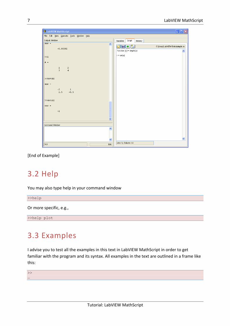
The“LabVIEWMathScriptWindow”isaninteractiveinterfaceinwhichyoucanenter.mfilescriptcommandsandseeimmediateresults,variablesandcommandshistory.Thewindowincludesacommand-lineinterfacewhereyoucanentercommandsone-by-oneforquickcalculations,scriptdebuggingorlearning.Alternatively,youcanenterandexecutegroupsofcommandsthroughascripteditorwindow.

Asyouwork,avariabledisplayupdatestoshowthegraphical/textualresultsandahistorywindowtracksyourcommands.Thehistoryviewfacilitatesalgorithmdevelopmentbyallowingyoutousetheclipboardtoreuseyourpreviouslyexecutedcommands.

Youcanusethe“LabVIEWMathScriptWindow”toentercommandsoneattime.Youalsocanenterbatchscriptsinasimpletexteditorwindow,loadedfromatextfile,orimportedfromaseparatetexteditor.The“LabVIEWMathScriptWindow”providesimmediatefeedbackinavarietyofforms,suchasgraphsandtext.

Example:

7 LabVIEWMathScript


[EndofExample]

3.2 HelpYoumayalsotypehelpinyourcommandwindow

>>help

Ormorespecific,e.g.,

>>help plot

3.3 ExamplesIadviseyoutotestalltheexamplesinthistextinLabVIEWMathScriptinordertogetfamiliarwiththeprogramanditssyntax.Allexamplesinthetextareoutlinedinaframelikethis:

>> …

8 LabVIEWMathScript


ThisiscommandsyoushouldwriteintheCommandWindow.

YoutypeallyourcommandsintheCommandWindow.Iwillusethesymbol“>>”toillustratethatthecommandsshouldbewrittenintheCommandWindow.

Example:Matrices

Definingthefollowingmatrix

𝐴 = 1 20 3

Thesyntaxisasfollows:

>> A = [1 2;0 3]

Or

>> A = [1,2;0,3]

Ifyou,foranexample,wanttofindtheanswerto

𝑎 + 𝑏,𝑤ℎ𝑒𝑟𝑒𝑎 = 4, 𝑏 = 3

>>a=4 >>b=3 >>a+b

MathScriptthenresponds:

ans = 7

MathScriptprovidesasimplewaytodefinesimplearraysusingthesyntax:“init:increment:terminator”.Forinstance:

>> array = 1:2:9 array = 1 3 5 7 9

Thecodedefinesavariablenamedarray(orassignsanewvaluetoanexistingvariablewiththenamearray)whichisanarrayconsistingofthevalues1,3,5,7,and9.Thatis,thearraystartsat1(theinitvalue),incrementswitheachstepfromthepreviousvalueby2(theincrementvalue),andstopsonceitreaches(ortoavoidexceeding)9(theterminatorvalue).

Theincrementvaluecanactuallybeleftoutofthissyntax(alongwithoneofthecolons),touseadefaultvalueof1.

>> ari = 1:5

9 LabVIEWMathScript


ari = 1 2 3 4 5

Thecodeassignstothevariablenamedarianarraywiththevalues1,2,3,4,and5,sincethedefaultvalueof1isusedastheincrementer.

Notethattheindexingisone-based,whichistheusualconventionformatricesinmathematics.Thisisatypicalforprogramminglanguages,whosearraysmoreoftenstartwithzero.

Matricescanbedefinedbyseparatingtheelementsofarowwithblankspaceorcommaandusingasemicolontoterminateeachrow.Thelistofelementsshouldbesurroundedbysquarebrackets:[].Parentheses:()areusedtoaccesselementsandsubarrays(theyarealsousedtodenoteafunctionargumentlist).

>> A = [16 3 2 13; 5 10 11 8; 9 6 7 12; 4 15 14 1] A = 16 3 2 13 5 10 11 8 9 6 7 12 4 15 14 1 >> A(2,3) ans = 11

Setsofindicescanbespecifiedbyexpressionssuchas"2:4",whichevaluatesto[2,3,4].Forexample,asubmatrixtakenfromrows2through4andcolumns3through4canbewrittenas:

>> A(2:4,3:4) ans = 11 8 7 12 14 1

Asquareidentitymatrixofsizencanbegeneratedusingthefunctioneye,andmatricesofanysizewithzerosoronescanbegeneratedwiththefunctionszerosandones,respectively.

>> eye(3) ans = 1 0 0 0 1 0 0 0 1 >> zeros(2,3) ans = 0 0 0 0 0 0 >> ones(2,3) ans =

10 LabVIEWMathScript


1 1 1 1 1 1

3.4 UsefulcommandsHerearesomeusefulcommands:

Command Description

eye(x), eye(x,y) Identitymatrixoforderx

ones(x), ones(x,y) Amatrixwithonlyones

zeros(x), zeros(x,y) Amatrixwithonlyzeros

diag([x y z]) Diagonalmatrix

size(A) DimensionofmatrixA

A’ InverseofmatrixA

CallingfunctionsInMathScriptMathScriptincludesmorethan800built-infunctionsthatyoucanuse,e.g.,inaprevioustaskyouusedtheplotfunction.

Example:Built-inFunctions

Giventhevector:

>>x=[1 2 5 6 8 9 3]

→Findthemeanvalueofthevectorx.

→Findtheminimumvalueofthevectorx.

→Findthemaximumvalueofthevectorx.

TheMathScriptCodeis:

x=[1 2 5 6 8 9 3] mean(x)



min(x) max(x)

[EndofExample]

User-DefinedFunctionsInMathScriptMathScriptincludesmorethan800built-infunctionsthatyoucanusebutsometimesyouneedtocreateyourownfunctions.

TodefineyourownfunctioninMathScript,usethefollowingsyntax:

function outputs = function_name(inputs) % documentation …

Hereistheprocedureforcreatingaauser-definedfunctioninMathScript:



ScriptsAscriptisasequenceofMathScriptcommandsthatyouwanttoperformtoaccomplishatask.Whenyouhavecreatedthescriptyoumaysaveitasam-fileforlateruse.

YoumayalsohavemultipleScriptWindowsopenatthesametimebyselecting“NewScriptEditor”intheFilemenu:



Thisgives:



3.5 FlowControlThischapterexplainsthebasicconceptsofflowcontrolinMathScript.

Thetopicsareasfollows:

• If-elsestatement• Switchandcasestatement• Forloop• Whileloop

3.5.1 If-elseStatement

Theifstatementevaluatesalogicalexpressionandexecutesagroupofstatementswhentheexpressionistrue.Theoptionalelseifandelsekeywordsprovidefortheexecutionofalternategroupsofstatements.Anendkeyword,whichmatchestheif,terminatesthelastgroupofstatements.Thegroupsofstatementsaredelineatedbythefourkeywords—nobracesorbracketsareinvolved.

Example:If-ElseStatement

Testthefollowingcode:

n=5 if n > 2 M = eye(n) elseif n < 2 M = zeros(n) else M = ones(n) end

[EndofExample]

3.5.2 SwitchandCaseStatement

Theswitchstatementexecutesgroupsofstatementsbasedonthevalueofavariableorexpression.Thekeywordscaseandotherwisedelineatethegroups.Onlythefirstmatchingcaseisexecuted.Theremustalwaysbeanendtomatchtheswitch.

Example:SwitchandCaseStatement


n=2 switch(n)



case 1 M = eye(n) case 2 M = zeros(n) case 3 M = ones(n) end

[EndofExample]

3.5.3 Forloop

Theforlooprepeatsagroupofstatementsafixed,predeterminednumberoftimes.Amatchingenddelineatesthestatements.

Example:ForLoop


m=5 for n = 1:m r(n) = rank(magic(n)); end r

[EndofExample]

3.5.4 Whileloop

Thewhilelooprepeatsagroupofstatementsanindefinitenumberoftimesundercontrolofalogicalcondition.Amatchingenddelineatesthestatements.

Example:WhileLoop


m=5; while m > 1 m = m - 1; zeros(m) end

[EndofExample]



3.6 PlottingThischapterexplainsthebasicconceptsofcreatingplotsinMathScript.

Topics:

• BasicPlotcommands

Example:Plotting

Functionplotcanbeusedtoproduceagraphfromtwovectorsxandy.Thecode:

x = 0:pi/100:2*pi; y = sin(x); plot(x,y)

producesthefollowingfigureofthesinefunction:

[EndofExample]

Example:Plotting

Three-dimensionalgraphicscanbeproducedusingthefunctionssurf,plot3ormesh.

[X,Y] = meshgrid(-10:0.25:10,-10:0.25:10); f = sinc(sqrt((X/pi).^2+(Y/pi).^2)); mesh(X,Y,f); axis([-10 10 -10 10 -0.3 1]) xlabel('{\bfx}')



ylabel('{\bfy}') zlabel('{\bfsinc} ({\bfR})') hidden off

Thiscodeproducesthefollowing3Dplot:

[EndofExample]

18

4 LinearAlgebraExamplesRequires:MathScriptRTModule

Linearalgebraisabranchofmathematicsconcernedwiththestudyofmatrices,vectors,vectorspaces(alsocalledlinearspaces),linearmaps(alsocalledlineartransformations),andsystemsoflinearequations.

MathScriptarewellsuitedforLinearAlgebra.

4.1 VectorsGivenavectorx

𝑥 =

𝑥2𝑥3⋮𝑥5

∈ 𝑅5

Example:Vectors

Giventhefollowingvector

𝑥 =123

>> x=[1; 2; 3] x = 1 2 3

TheTransposeofvectorx:

𝑥8 = 𝑥2 𝑥3 ⋯ 𝑥5 ∈ 𝑅2:5

>> x' ans = 1 2 3

[EndofExample]

19 LinearAlgebraExamples


TheLengthofvectorx:

𝑥 = 𝑥8𝑥 = 𝑥23 + 𝑥33 + ⋯+ 𝑥53

Orthogonality:

𝑥8𝑦 = 0

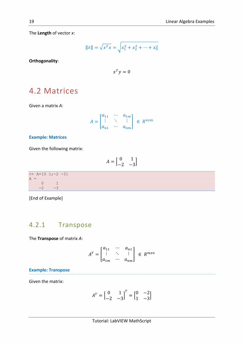
4.2 MatricesGivenamatrixA:

𝐴 =𝑎22 ⋯ 𝑎2<⋮ ⋱ ⋮𝑎52 ⋯ 𝑎5<

∈ 𝑅5:<

Example:Matrices

Giventhefollowingmatrix:

𝐴 = 0 1−2 −3

>> A=[0 1;-2 -3] A = 0 1 -2 -3

[EndofExample]

4.2.1 Transpose

TheTransposeofmatrixA:

𝐴8 =𝑎22 ⋯ 𝑎52⋮ ⋱ ⋮

𝑎2< ⋯ 𝑎5<∈ 𝑅<:5

Example:Transpose

Giventhematrix:

𝐴8 = 0 1−2 −3

8= 0 −2

1 −3



>> A' ans = 0 -2 1 -3

[EndofExample]

4.2.2 Diagonal

TheDiagonalelementsofmatrixAisthevector

𝑑𝑖𝑎𝑔(𝐴) =

𝑎22𝑎33⋮𝑎DD

∈ 𝑅DEFGH(:,<)

Example:Diagonal

FindthediagonalelementsofmatrixA:

>> diag(A) ans = 0 -3

[EndofExample]

TheDiagonalmatrixΛisgivenby:

Λ =

𝜆2 0 ⋯ 00 𝜆3 ⋯ 0⋮ ⋮ ⋱ ⋮0 0 ⋯ 𝜆5

∈ 𝑅5:5

GiventheIdentitymatrixI:

𝐼 =

1 0 ⋯ 00 1 ⋯ 0⋮ ⋮ ⋱ ⋮0 0 ⋯ 1

∈ 𝑅5:<

Example:IdentityMatrix

Getthe3x3Identitymatrix:

>> eye(3) ans = 1 0 0



0 1 0 0 0 1

[EndofExample]

4.2.3 Triangular

LowerTriangularmatrixL:

𝐿 =. 0 0⋮ ⋱ 0. ⋯ .

UpperTriangularmatrixU:

𝑈 =. ⋯ .0 ⋱ ⋮0 0 .

4.2.4 MatrixMultiplication

Giventhematrices 𝐴 ∈ 𝑅5:< and 𝐵 ∈ 𝑅<:D,then

𝐶 = 𝐴𝐵 ∈ 𝑅5:D

where

𝑐RS = 𝑎RT𝑏TS

5

TE2

Example:MatrixMultiplication

Matrixmultiplication:

>> A=[0 1;-2 -3] A = 0 1 -2 -3 >> B=[1 0;3 -2] B = 1 0 3 -2 >> A*B ans = 3 -2 -11 6

[EndofExample]



Note!

𝐴𝐵 ≠ 𝐵𝐴

𝐴 𝐵𝐶 = 𝐴𝐵 𝐶

𝐴 + 𝐵 𝐶 = 𝐴𝐶 + 𝐵𝐶

𝐶 𝐴 + 𝐵 = 𝐶𝐴 + 𝐶𝐵

4.2.5 MatrixAddition

Giventhematrices 𝐴 ∈ 𝑅5:< and 𝐵 ∈ 𝑅5:<,then

𝐶 = 𝐴 + 𝐵 ∈ 𝑅5:<

Example:MatrixAddition

Matrixaddition:

>> A=[0 1;-2 -3] >> B=[1 0;3 -2] >> A+B ans = 1 1 1 -5

[EndofExample]

4.2.6 Determinant

Givenamatrix 𝐴 ∈ 𝑅5:5,thentheDeterminantisgiven:

det 𝐴 = 𝐴

Givena2x2matrix

𝐴 =𝑎22 𝑎23𝑎32 𝑎33 ∈ 𝑅3:3

Then

det 𝐴 = 𝐴 = 𝑎22𝑎33 − 𝑎32𝑎23



Example:Determinant

Findthedeterminant:

A = 0 1 -2 -3 >> det(A) ans = 2

Noticethat

det 𝐴𝐵 = det 𝐴 det 𝐵

and

det 𝐴8 = det(𝐴)

[EndofExample]

Example:Determinant

Determinants:

>> det(A*B) ans = -4 >> det(A)*det(B) ans = -4 >> det(A') ans = 2 >> det(A) ans = 2

[EndofExample]

4.2.7 InverseMatrices

Theinverseofaquadraticmatrix 𝐴 ∈ 𝑅5:5 isdefinedby:

𝐴Y2

if



𝐴𝐴Y2 = 𝐴Y2𝐴 = 𝐼

Fora2x2matrixwehave:

𝐴 =𝑎22 𝑎23𝑎32 𝑎33 ∈ 𝑅3:3

Theinverse 𝐴Y2 isgivenby

𝐴Y2 =1

det(𝐴)𝑎33 −𝑎23−𝑎32 𝑎22 ∈ 𝑅3:3

Example:InverseMatrices

Inversematrix:

A = 0 1 -2 -3 >> inv(A) ans = -1.5000 -0.5000 1.0000 0

[EndofExample]

Noticethat:

𝐴𝐴Y2 = 𝐴Y2𝐴 = 𝐼

→ProvethisinMathScript

4.3 EigenvaluesGiven 𝐴 ∈ 𝑅5:5,thentheEigenvaluesisdefinedas:

det 𝜆𝐼 − 𝐴 = 0

Example:Eigenvalues

FindtheEigenvalues:

A = 0 1 -2 -3 >> eig(A) ans = -1 -2



[EndofExample]

4.4 SolvingLinearEquationsGiventhelinearequation

𝐴𝑥 = 𝑏

withthesolution:

𝑥 = 𝐴Y2𝑏

(AssumingthattheinverseofAexists)

Example:SolvingLinearEquations

Solvingthefollowingequation:

Theequations

𝑥2 + 2𝑥3 = 53𝑥2 + 4𝑥3 = 6

maybewritten

𝐴𝑥 = 𝑏

1 23 4

𝑥2𝑥3 = 5

6

where

𝐴 = 1 23 4

𝑥 =𝑥2𝑥3

𝑏 = 56

Thesolutionis:

A = 1 2 3 4 >> b=[5;6] b = 5 6 >> x=inv(A)*b



x = -4.0000 4.5000

InMathScriptyoucouldalsowrite“x=A\b”,whichshouldgivethesameanswer.ThissyntaxcanalsobeusedwhentheinverseofAdon’texists.

[EndofExample]

Example:SolvingLinearEquations

Illegaloperation:

>> A=[1 2;3 4;7 8] >> x=inv(A)*b ??? Error using ==> inv Matrix must be square. >> x=A\b x = -3.5000 4.1786

[EndofExample]

4.5 LUfactorizationLUfactorizationof 𝐴 ∈ 𝑅5:< isgivenby

𝐴 = 𝐿𝑈

where

Lisalowertriangularmatrix

Uisauppertriangularmatrix

TheMathScriptsyntaxis[L,U]=lu(A)

Example:LUFactorization

FindLandU:

>> A=[1 2;3 4] >> [L,U]=lu(A) L = 0.3333 1.0000 1.0000 0 U = 3.0000 4.0000



0 0.6667

[EndofExample]

OrsometimesLUfactorizationof 𝐴 ∈ 𝑅5:< isgivenby

𝐴 = 𝐿𝑈 = 𝐿𝐷𝑈

where

Disadiagonalmatrix

TheMathScriptsyntaxis[L,U,P]=lu(A)

Example:LUFactorization

FindL,UandP:

>> A=[1 2;3 4] A = 1 2 3 4 >> [L,U,P]=lu(A) L = 1.0000 0 0.3333 1.0000 U = 3.0000 4.0000 0 0.6667 P = 0 1 1 0

[EndofExample]

4.6 TheSingularValueDecomposition(SVD)TheSingularvalueDecomposition(SVD)ofthematrix 𝐴 ∈ 𝑅5:< isgivenby

𝐴 = 𝑈𝑆𝑉8

where

Uisaorthogonalmatrix

Visaorthogonalmatrix

Sisadiagonalsingularmatrix



Example:SVDDecomposition

FindS,VandD:

>> A=[1 2;3 4]; >> [U,S,V] = svd(A) U = -0.4046 -0.9145 -0.9145 0.4046 S = 5.4650 0 0 0.3660 V = -0.5760 0.8174 -0.8174 -0.5760

[EndofExample]

4.7 Commands

Command Description

[L,U]=lu(A)

[L,U,P]=lu(A)LUFactorization

[U,S,V] = svd(A) SingularValueDecomposition(SVD)

29

5 ControlDesignandSimulation

UsingLabVIEWMathScriptforControlDesignpurposesyouneedtoinstallthe“ControlDesignandSimulationModule”inadditiontothe“MathScriptRTModule”itself.

UsetheControlDesignMathScriptRTModulefunctionstodesign,analyze,andsimulatelinearcontrollermodelsusingatext-basedlanguage.ThefollowingisalistofControlDesignMathScriptRTModuleclassesoffunctionsandcommandsthatLabVIEWMathScriptsupports.

GettinghelpaboutMathScriptfunctionsregardingtheControlDesignToolkit(CDT),type“helpcdt”intheCommandWindowintheMathScriptenvironment.

Thefollowingfunctionclassesexist:

Wewillgothroughsomeoftheclassesandfunctionindetailbelow:

5.1 State-spacemodelsandTransferfunctionsMathScriptofferslotsoffunctionsfordefiningandmanipulatestate-spacemodelsandtransferfunctions.



Class:contruct

Description:

Usefunctionsintheconstructclasstoconstructlineartime-invariantsystemmodelsandtoconvertbetweenmodelforms.

Belowweseethedifferentfunctionsavailableintheconstructclass:

Belowwewillgivesomeexamplesofhowtousethemostimportfunctionsinthisclass.

5.1.1 PID

Currently,theProportional-Integral-Derivative(PID)algorithmisthemostcommoncontrolalgorithmusedinindustry.

InPIDcontrol,youmustspecifyaprocessvariableandasetpoint.Theprocessvariableisthesystemparameteryouwanttocontrol,suchastemperature,pressure,orflowrate,andthesetpointisthedesiredvaluefortheparameteryouarecontrolling.

APIDcontrollerdeterminesacontrolleroutputvalue,suchastheheaterpowerorvalveposition.Thecontrollerappliesthecontrolleroutputvaluetothesystem,whichinturndrivestheprocessvariabletowardtheset-pointvalue.

ThenthePIDcontrollercalculatesthecontrolleraction,u(t):

𝑢(𝑡) = 𝐾b 𝑒 +1𝑇d

𝑒𝑑𝑡 + 𝑇e𝑑𝑒𝑑𝑡

f

g

Where

𝐾b Controllergain

𝑇d Integraltime



𝑇e Derivativetime

And 𝑒 istheerror

𝑒 = 𝑆𝑃 − 𝑃𝑉

SP–Setpoint

PV–ProcessVariable

Function:pid

Description:

Constructsaproportional-integral-derivative(PID)controllermodelineitherparallel,series,oracademicform.

Examples:

Kc = 0.5; Ti = 0.25; SysOutTF = pid(Kc, Ti, 'academic');

[EndofExample]

5.1.2 State-spacemodel

Astate-spacemodelisjustastructuredformorrepresentationofthedifferentialequationsforasystem.

AlinearState-spacemodel:

𝑥 = 𝐴𝑥 + 𝐵𝑢

𝑦 = 𝐶𝑥 + 𝐷𝑢

wherexisthestatevectoranduistheinputvector.Aiscalledthesystem-matrix,andissquareinallcases.

Example:

Thedifferentialequations:



𝑥2 = −2𝑥2 + 6𝑢

𝑥3 = 2𝑥2

Maybewrittenonstate-spaceform:

𝑥2𝑥3

= −2 02 0

𝑥2𝑥3 + 6

0 𝑢

Function:ss

Description:

Thisfunctionconstructsacontinuousordiscretelinearsystemmodelinstate-spaceform.Youalsocanusethisfunctiontoconverttransferfunctionandzero-pole-gainmodelstostate-spaceform.

Examples:

% Creates a state-space model A = eye(2) B = [0; 1] C = B' SysOutSS = ss(A, B, C) % Converts a zero-pole-gain model to state-space form z = 1 p = [1, -1] k = 1 SysIn = zpk(z, p, k) SysOutSS = ss(SysIn)

[EndofExample]

5.1.3 Transferfunction

ThetransferfunctionofalinearsystemisdefinedastheratiooftheLaplacetransformoftheoutputvariabletotheLaplacetransformoftheinputvariable.

𝐻 𝑆 =𝑦(𝑠)𝑢(𝑠)

Functiontf

Description:



Thisfunctioncreatesacontinuousordiscretelinearsystemmodelintransferfunctionform.Youalsocanusethisfunctiontoconvertzero-pole-gainandstate-spacemodelstotransferfunctionform.

Examples:

>>s = tf('s')

Thisspecifiesthatyouwanttocreatethecontinuoustransferfunctions/1.Afteryouenterthiscommand,youcanuseLabVIEWMathScriptoperandsonthistransferfunctiontodefineazero-pole-gainortransferfunctionmodel.

SysOutZPK = 4*(s + 2) / (s + 1)

Thisexampleconstructsazero-pole-gainmodelwithagainof4,azeroat-2,andapoleat-1.

SysOutTF = (3*(s*s*s) + 2) / (4*(s*s*s*s) + 8)

Thisexampleconstructsthetransferfunctionmodel3s^3+2/4s^4+8.

[EndofExample]

5.1.4 FirstOrderSystems

Thefollowingtransferfunctiondefinesafirstordersystem:

𝐻 𝑠 =𝐾

𝑇𝑠 + 1

Where

𝐾 isthegain

𝑇 istheTimeconstant

Functionsys_order1

Description:

Thisfunctionconstructsthecomponentsofafirst-ordersystemmodelbasedonagain,timeconstant,anddelaythatyouspecify.Youcanusethisfunctiontocreateeitherastate-spacemodeloratransferfunctionmodel,dependingontheoutputparametersyouspecify.



Inputs:

KSpecifiesthegainmatrix.Kisarealmatrix.

tauSpecifiesthetimeconstant,inseconds,whichisthetimerequiredforthemodeloutputtoreach63%ofitsfinalvalue.Thedefaultvalueis0.

delaySpecifiestheresponsedelayofthemodel,inseconds.Thedefaultvalueis0.

Examples:

K = 0.5; tau = 1.5; SysOutTF = sys_order1(K, tau);

[EndofExample]

5.1.5 SecondOrderSystems

Astandardsecondordertransferfunctionmodelmaybewrittenlikethis:

𝐻 𝑠 =𝑦(𝑠)𝑢(𝑠) =

𝐾𝜔g3

𝑠3 + 2𝜁𝜔g𝑠 + 𝜔g3=

𝐾𝑠𝜔g

3+ 2𝜁 𝑠

𝜔g+ 1

Where

𝐾 isthegain

𝜁(zetaistherelativedampingfactor

𝜔g[rad/s]istheundampedresonancefrequency.

Functionsys_order2

Description:

Thisfunctionconstructsthecomponentsofasecond-ordersystemmodelbasedonadampingratioandnaturalfrequencyyouspecify.Youcanusethisfunctiontocreateeitherastate-spacemodeloratransferfunctionmodel,dependingontheoutputparametersyouspecify.

Example:

Examplesofhowtousethesys_order2function:



dr = 0.5 wn = 20 [num, den] = sys_order2(wn, dr) SysTF = tf(num, den) [A, B, C, D] = sys_order2(wn, dr) SysSS = ss(A, B, C, D)

[EndofExample]

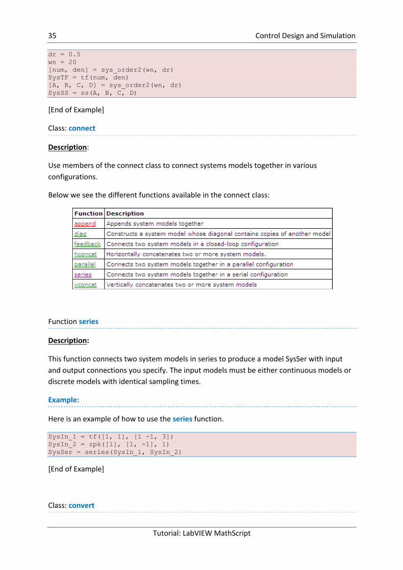
Class:connect

Description:

Usemembersoftheconnectclasstoconnectsystemsmodelstogetherinvariousconfigurations.

Belowweseethedifferentfunctionsavailableintheconnectclass:

Functionseries

Description:

ThisfunctionconnectstwosystemmodelsinseriestoproduceamodelSysSerwithinputandoutputconnectionsyouspecify.Theinputmodelsmustbeeithercontinuousmodelsordiscretemodelswithidenticalsamplingtimes.

Example:

Hereisanexampleofhowtousetheseriesfunction.

SysIn_1 = tf([1, 1], [1 -1, 3]) SysIn_2 = zpk([1], [1, -1], 1) SysSer = series(SysIn_1, SysIn_2)

[EndofExample]

Class:convert



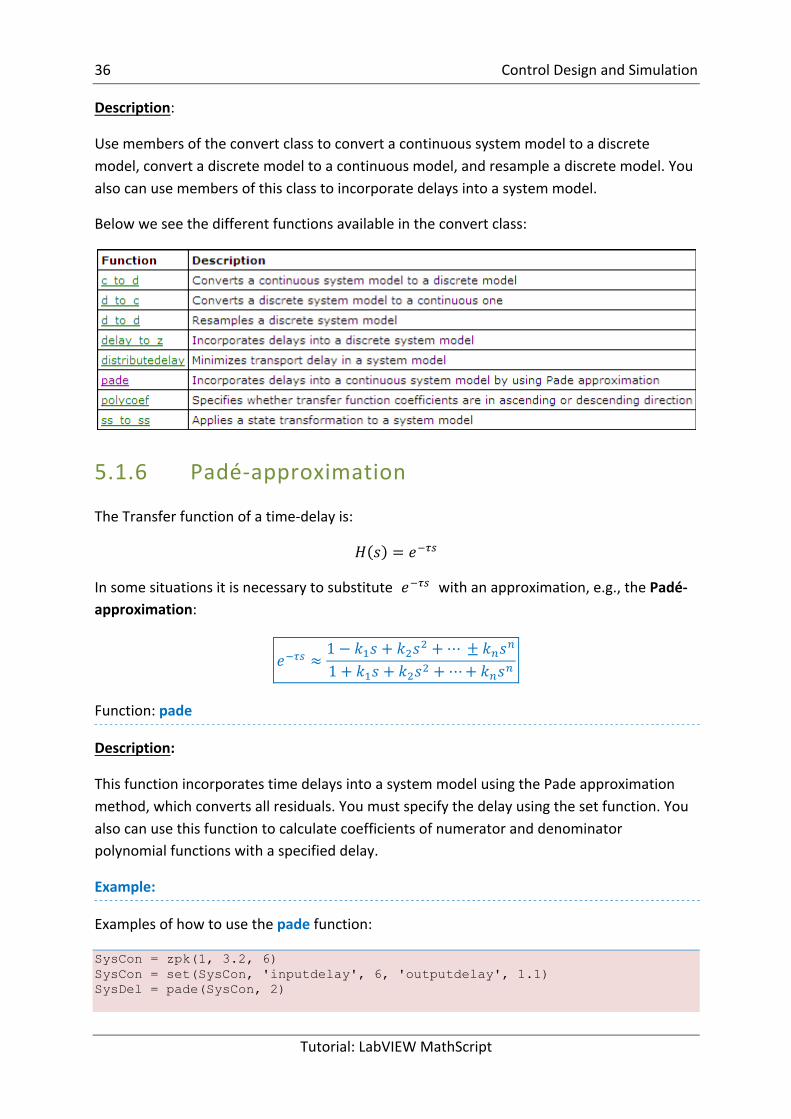
Description:

Usemembersoftheconvertclasstoconvertacontinuoussystemmodeltoadiscretemodel,convertadiscretemodeltoacontinuousmodel,andresampleadiscretemodel.Youalsocanusemembersofthisclasstoincorporatedelaysintoasystemmodel.

Belowweseethedifferentfunctionsavailableintheconvertclass:

5.1.6 Padé-approximation

TheTransferfunctionofatime-delayis:

𝐻 𝑠 = 𝑒Ymn

Insomesituationsitisnecessarytosubstitute 𝑒Ymn withanapproximation,e.g.,thePadé-approximation:

𝑒Ymn ≈1 − 𝑘2𝑠 + 𝑘3𝑠3 + ⋯± 𝑘5𝑠5

1 + 𝑘2𝑠 + 𝑘3𝑠3 + ⋯+ 𝑘5𝑠5

Function:pade

Description:

ThisfunctionincorporatestimedelaysintoasystemmodelusingthePadeapproximationmethod,whichconvertsallresiduals.Youmustspecifythedelayusingthesetfunction.Youalsocanusethisfunctiontocalculatecoefficientsofnumeratoranddenominatorpolynomialfunctionswithaspecifieddelay.

Example:

Examplesofhowtousethepadefunction:

SysCon = zpk(1, 3.2, 6) SysCon = set(SysCon, 'inputdelay', 6, 'outputdelay', 1.1) SysDel = pade(SysCon, 2)



delay = 1.2 order = 3 [num, den] = pade(delay, order)

[EndofExample]

5.2 FrequencyResponseAnalysisThefrequencyresponseofasystemisafrequencydependentfunctionwhichexpresseshowasinusoidalsignalofagivenfrequencyonthesysteminputistransferredthroughthesystem.Eachfrequencycomponentisasinusoidalsignalhavingacertainamplitudeandacertainfrequency.

Thefrequencyresponseisanimportanttoolforanalysisanddesignofsignalfiltersandforanalysisanddesignofcontrolsystems.

Thefrequencyresponsecanfoundexperimentallyorfromatransferfunctionmodel.

Thefrequencyresponseofasystemisdefinedasthesteady-stateresponseofthesystemtoasinusoidalinputsignal.Whenthesystemisinsteady-stateitdiffersfromtheinputsignalonlyinamplitude(A)andphaseangle(ω).

Ifwehavetheinputsignal:

𝑢 𝑡 = 𝑈𝑠𝑖𝑛𝜔𝑡

Thesteady-stateoutputsignalwillbe:

𝑦 𝑡 = 𝑈𝐴sin(𝜔𝑡 + 𝜙)

Aand 𝜙 isafunctionofthefrequencyωsowemaywrite 𝐴 = 𝐴 𝜔 ,𝜙 = 𝜙(𝜔)

Foratransferfunction

𝐻 𝑆 =𝑦(𝑠)𝑢(𝑠)

Wehave:

𝐴 𝜔 = 𝐻(𝑗𝜔)

𝜙 𝜔 = ∠𝐻(𝑗𝜔)

Where 𝐻(𝑗𝜔) isthefrequencyresponseofthesystem,i.e.,wemayfindthefrequencyresponsebysetting 𝑠 = 𝑗𝜔 inthetransferfunction.



5.2.1 BodeDiagram

Bodediagramsareusefulinfrequencyresponseanalysis.TheBodediagramconsistsof2diagrams,theBodemagnitudediagram, 𝐴(𝜔) andtheBodephasediagram, 𝜙(𝜔).

The 𝐴(𝜔)-axisisindecibel(dB)

Wherethedecibelvalueofxiscalculatedas: 𝑥 𝑑𝐵 = 20𝑙𝑜𝑔2g𝑥

The 𝜙(𝜔)-axisisindegrees(notradians)

Function:bode

Description:

ThisfunctioncreatestheBodemagnitudeandBodephaseplotsofasystemmodel.Youalsocanusethisfunctiontoreturnthemagnitudeandphasevaluesofamodelatfrequenciesyouspecify.Ifyoudonotspecifyanoutput,thisfunctioncreatesaplot.

Examples:

Wehavethefollowingtransferfunction

𝐻 𝑠 =𝑦(𝑠)𝑢(𝑠) =

1𝑠 + 1

WewanttoplottheBodediagramforthistransferfunction:

InMathScriptwecouldwrite:



num=[1]; den=[1,1]; H1=tf(num,den) bode(H1)

[EndofExample]

Function:margin

Description:

Thisfunctioncalculatesand/orplotsthesmallestgainandphasemarginsofasingle-inputsingle-output(SISO)systemmodel.

Thegainmarginindicateswherethefrequencyresponsecrossesat0decibels(“crossoverfrequency”, 𝜔b).

𝐻(𝑗𝑤b)

𝜔b isalsothebandwidthofthesystem

Thephasemarginindicateswherethefrequencyresponsecrosses-180degrees(“crossoverfrequency”, 𝜔2�g).

∠𝐻(𝑗𝑤2�g)

Examples:

Thefollowingexampleillustratestheuseofthemarginfunction.

num = [1] den = [1, 5, 6] H = tf(num, den) margin(H)

[EndofExample]

Example:

Giventhefollowingsystem:

𝐻 𝑆 =1

𝑠 𝑠 + 1 3



WewanttoplottheBodediagramandfindthecrossover-frequenciesforthesystemusingMathScript.

Weusethefollowingfunctions:tf,bode,marginsandmargin.

• gmfisthegainmarginfrequencies,inradians/second.Againmarginfrequencyindicateswherethemodelphasecrosses-180degrees.

• gmReturnsthegainmarginsofthesystem. • pmfReturnsthephasemarginfrequencies,inradians/second.Aphasemargin

frequencyindicateswherethemodelmagnitudecrosses0decibels. • pmReturnsthephasemarginsofthesystem.• Weget:

BelowweseetheBodediagramwiththecrossover-frequencyandthegainmarginandphasemarginforthesystemplottedin:



[EndofExample]

TimeResponseClass:timeresp

Description:

Usemembersofthetimerespclasstocreategenericlinearsimulationsandtimedomainplotsforstepinputs,impulseinputs,andinitialconditionresponses.

Belowweseethedifferentfunctionsavailableinthetimerespclass:

Function:step

Description:



Thisfunctioncreatesastepresponseplotofthesystemmodel.Youalsocanusethisfunctiontoreturnthestepresponseofthemodeloutputs.Ifthemodelisinstate-spaceform,youalsocanusethisfunctiontoreturnthestepresponseofthemodelstates.Thisfunctionassumestheinitialmodelstatesarezero.Ifyoudonotspecifyanoutput,thisfunctioncreatesaplot.

Example:

Giventhefollowingsystem:

𝐻 𝑠 =𝑠 + 1

𝑠3 − 𝑠 + 3

Wewillplotthetimeresponseforthetransferfunctionusingthestepfunction

Theresultisasfollows:

TheMathScriptcode:

H = tf([1, 1], [1, -1, 3]) step(H)

[EndofExample]

43

6 MathScriptNodeThe“MathScriptNode”offersanintuitivemeansofcombininggraphicalandtextualcodewithinLabVIEW.Thefigurebelowshowsthe“MathScriptNode”ontheblockdiagram,representedbythebluerectangle.Using“MathScriptNodes”,youcanenter.mfilescripttextdirectlyorimportitfromatextfile.

YoucandefinenamedinputsandoutputsontheMathScriptNodebordertospecifythedatatotransferbetweenthegraphicalLabVIEWenvironmentandthetextualMathScriptcode.

Youcanassociate.mfilescriptvariableswithLabVIEWgraphicalprogramming,bywiringNodeinputsandoutputs.Thenyoucantransferdatabetween.mfilescriptswithyourgraphicalLabVIEWprogramming.Thetextual.mfilescriptscannowaccessfeaturesfromtraditionalLabVIEWgraphicalprogramming.

TheMathScriptNodeisavailablefromLabVIEWfromtheFunctionsPalette:Mathematics→Scripts&Formulas

44 MathScriptNode


IfyouclickCtrl+HyougethelpabouttheMathScriptNode:

Click“Detailedhelp”inordertogetmoreinformationabouttheMathScriptNode.

UsetheNIExampleFinderinordertofindexamples:

45 MathScriptNode


6.1 TransferringMathScriptNodesbetweenComputers

IfascriptinaMathScriptNodecallsauser-definedfunction,LabVIEWusesthedefaultsearchpathlisttolinkthefunctioncalltothespecified.mfile.AfteryouconfigurethedefaultsearchpathlistandsavetheVIthatcontainstheMathScriptNode,youdonotneedtoreconfiguretheMathScriptsearchpathlistwhenyouopentheVIonadifferentcomputerbecauseLabVIEWlooksforthe.mfileinthedirectorywherethe.mfilewaslocatedwhenyoulastsavedtheVI.However,youmustmaintainthesamerelativepathbetweentheVIandthe.mfile.

6.2 ExamplesExample:UsingtheMathScriptNode

HereisanexampleofhowyouusetheMathScriptNode.Ontheleftborderyouconnectinputvariablestothescript,ontherightborderyouhaveoutputvariables.Right-clickontheborderandselect“AddInput”or“AddOutput”.

46 MathScriptNode


[EndofExample]

Example:CallingaWindowsDLL:

[EndofExample]

Example:Usingm-filesintheMathScriptNode:

UsetheLabVIEWMathScripttocreateam-filescript(oryoumayuseMATLABtocreatethesamescript):

47 MathScriptNode


Right-clickontheborderoftheMathScriptNodeandselect“Import”,andthenselectthem-fileyouwanttoimportintotheNode.

48 MathScriptNode


Right-clickontherightborderandselect“AddOutput”.Thenright-clickontheoutputvariableandselect“CreateIndicator”.

BlockDiagram:

Theresultisasfollows(clicktheRunbutton):

Ifyou,e.g.,addthefollowingcommandintheMathScriptNode:plot(x),thefollowingwindowappears:

[EndofExample]

49 MathScriptNode


6.3 ExercisesUsetheMathScriptNodeandtestthesameexamplesyoudidinapreviouschapter(Chapter4-“LinearAlgebraExamples”).

50

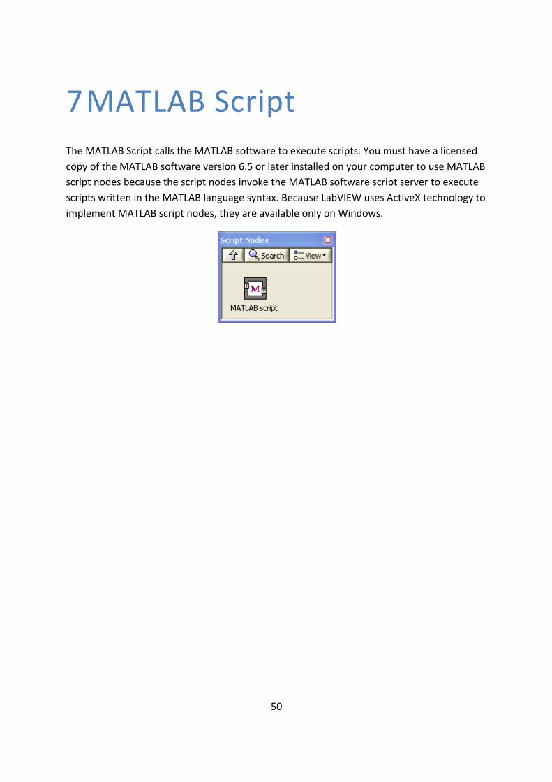
7 MATLABScriptTheMATLABScriptcallstheMATLABsoftwaretoexecutescripts.YoumusthavealicensedcopyoftheMATLABsoftwareversion6.5orlaterinstalledonyourcomputertouseMATLABscriptnodesbecausethescriptnodesinvoketheMATLABsoftwarescriptservertoexecutescriptswrittenintheMATLABlanguagesyntax.BecauseLabVIEWusesActiveXtechnologytoimplementMATLABscriptnodes,theyareavailableonlyonWindows.

51

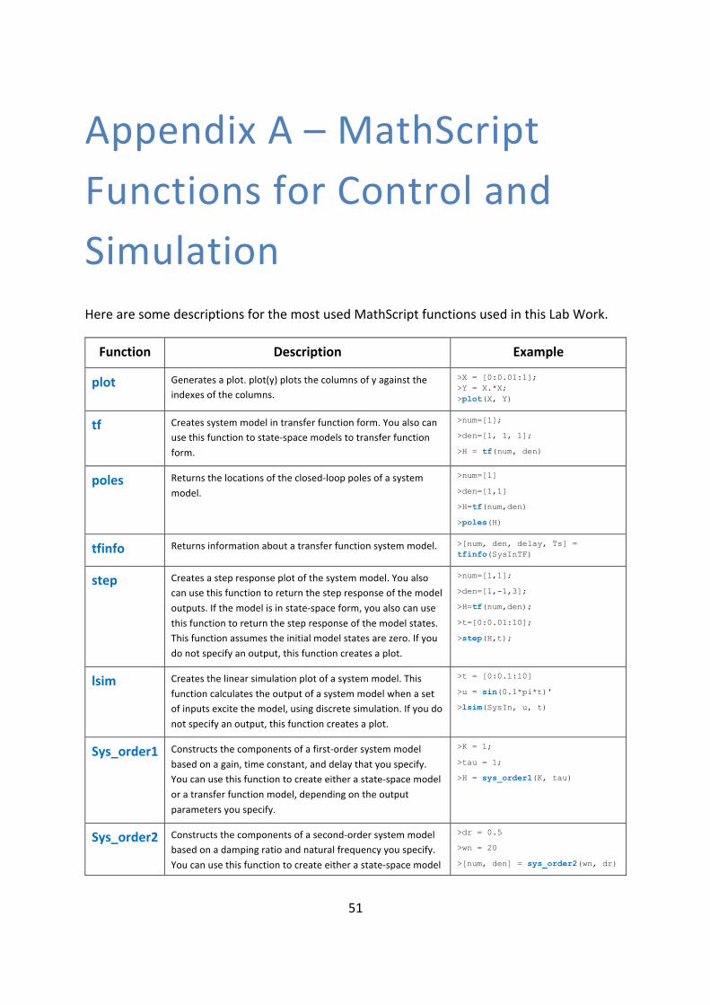
AppendixA–MathScriptFunctionsforControlandSimulationHerearesomedescriptionsforthemostusedMathScriptfunctionsusedinthisLabWork.

Function Description Example

plot Generatesaplot.plot(y)plotsthecolumnsofyagainsttheindexesofthecolumns.

>X = [0:0.01:1]; >Y = X.*X; >plot(X, Y)

tf Createssystemmodelintransferfunctionform.Youalsocanusethisfunctiontostate-spacemodelstotransferfunctionform.

>num=[1];

>den=[1, 1, 1];

>H = tf(num, den)

poles Returnsthelocationsoftheclosed-looppolesofasystemmodel.

>num=[1]

>den=[1,1]

>H=tf(num,den)

>poles(H)

tfinfo Returnsinformationaboutatransferfunctionsystemmodel. >[num, den, delay, Ts] = tfinfo(SysInTF)

step Createsastepresponseplotofthesystemmodel.Youalsocanusethisfunctiontoreturnthestepresponseofthemodeloutputs.Ifthemodelisinstate-spaceform,youalsocanusethisfunctiontoreturnthestepresponseofthemodelstates.Thisfunctionassumestheinitialmodelstatesarezero.Ifyoudonotspecifyanoutput,thisfunctioncreatesaplot.

>num=[1,1];

>den=[1,-1,3];

>H=tf(num,den);

>t=[0:0.01:10];

>step(H,t);

lsim Createsthelinearsimulationplotofasystemmodel.Thisfunctioncalculatestheoutputofasystemmodelwhenasetofinputsexcitethemodel,usingdiscretesimulation.Ifyoudonotspecifyanoutput,thisfunctioncreatesaplot.

>t = [0:0.1:10]

>u = sin(0.1*pi*t)'

>lsim(SysIn, u, t)

Sys_order1 Constructsthecomponentsofafirst-ordersystemmodelbasedonagain,timeconstant,anddelaythatyouspecify.Youcanusethisfunctiontocreateeitherastate-spacemodeloratransferfunctionmodel,dependingontheoutputparametersyouspecify.

>K = 1;

>tau = 1;

>H = sys_order1(K, tau)

Sys_order2 Constructsthecomponentsofasecond-ordersystemmodelbasedonadampingratioandnaturalfrequencyyouspecify.Youcanusethisfunctiontocreateeitherastate-spacemodel

>dr = 0.5

>wn = 20

>[num, den] = sys_order2(wn, dr)

52 Error!Referencesourcenotfound.


oratransferfunctionmodel,dependingontheoutputparametersyouspecify.

>SysTF = tf(num, den)

>[A, B, C, D] = sys_order2(wn, dr)

>SysSS = ss(A, B, C, D)

damp Returnsthedampingratiosandnaturalfrequenciesofthepolesofasystemmodel.

>[dr, wn, p] = damp(SysIn)

pid Constructsaproportional-integral-derivative(PID)controllermodelineitherparallel,series,oracademicform.RefertotheLabVIEWControlDesignUserManualforinformationaboutthesethreeforms.

>Kc = 0.5;

>Ti = 0.25;

>SysOutTF = pid(Kc, Ti, 'academic');

conv Computestheconvolutionoftwovectorsormatrices. >C1 = [1, 2, 3];

>C2 = [3, 4];

>C = conv(C1, C2)

series ConnectstwosystemmodelsinseriestoproduceamodelSysSerwithinputandoutputconnectionsyouspecify

>Hseries = series(H1,H2)

feedback Connectstwosystemmodelstogethertoproduceaclosed-loopmodelusingnegativeorpositivefeedbackconnections

>SysClosed = feedback(SysIn_1, SysIn_2)

ss Constructsamodelinstate-spaceform.Youalsocanusethisfunctiontoconverttransferfunctionmodelstostate-spaceform.

>A = eye(2)

>B = [0; 1]

>C = B'

>SysOutSS = ss(A, B, C)

ssinfo Returnsinformationaboutastate-spacesystemmodel. >A = [1, 1; -1, 2]

>B = [1, 2]'

>C = [2, 1]

>D = 0

>SysInSS = ss(A, B, C, D)

>[A, B, C, D, Ts] = ssinfo(SysInSS)

pade IncorporatestimedelaysintoasystemmodelusingthePadeapproximationmethod,whichconvertsallresiduals.Youmustspecifythedelayusingthesetfunction.Youalsocanusethisfunctiontocalculatecoefficientsofnumeratoranddenominatorpolynomialfunctionswithaspecifieddelay.

>[num, den] = pade(delay, order)

>[A, B, C, D] = pade(delay, order)

bode CreatestheBodemagnitudeandBodephaseplotsofasystemmodel.Youalsocanusethisfunctiontoreturnthemagnitudeandphasevaluesofamodelatfrequenciesyouspecify.Ifyoudonotspecifyanoutput,thisfunctioncreatesaplot.

>num=[4];

>den=[2, 1];

>H = tf(num, den)

>bode(H)

bodemag CreatestheBodemagnitudeplotofasystemmodel.Ifyoudonotspecifyanoutput,thisfunctioncreatesaplot.

>[mag, wout] = bodemag(SysIn)

>[mag, wout] = bodemag(SysIn, [wmin wmax])

>[mag, wout] = bodemag(SysIn, wlist)

margin Calculatesand/orplotsthesmallestgainandphasemarginsofasingle-inputsingle-output(SISO)systemmodel.Thegainmarginindicateswherethefrequencyresponsecrossesat0decibels.Thephasemarginindicateswherethefrequencyresponsecrosses-180degrees.UsethemarginsfunctiontoreturnallgainandphasemarginsofaSISOmodel.

>num = [1]

>den = [1, 5, 6]

>H = tf(num, den)

margin(H)

53 Error!Referencesourcenotfound.


margins Calculatesallgainandphasemarginsofasingle-inputsingle-output(SISO)systemmodel.Thegainmarginsindicatewherethefrequencyresponsecrossesat0decibels.Thephasemarginsindicatewherethefrequencyresponsecrosses-180degrees.UsethemarginfunctiontoreturnonlythesmallestgainandphasemarginsofaSISOmodel.

>[gmf, gm, pmf, pm] = margins(H)

Formoredetailsaboutthesefunctions,type“helpcdt”togetanoverviewofallthefunctionsusedforControlDesignandSimulation.Fordetailedhelpaboutonespecificfunction,type“help<function_name>”.

Plotsfunctions:Herearesomeusefulfunctionsforcreatingplots:plot,figure,subplot,grid,axis,title,xlabel,ylabel,semilogx–formoreinformationabouttheplotsfunction,type“helpplots”.

Hans-PetterHalvorsen,M.Sc.

E-mail:[email protected]

Blog:http://home.hit.no/~hansha/

UniversityCollegeofSoutheastNorway

www.usn.no

tutorial: labview mathscript

Documents