tutorial - africa - vito

Tutorial SPIRITS Version 1.1.1 – February 2013

Revised Draft – June 2013

Carolien Tote, Sven Gilliams, Dominique Haesen, Felix Rembold, Ferdinando Urbano

SPIRITS Tutorial

Introduction 2

Table of Contents Introduction ..................................................................................................................... 5

Part 1 The SPIRITS environment .................................................................................... 7

Exercise 1-1 Installation of SPIRITS .................................................................................................. 8

Exercise 1-2 Getting started .......................................................................................................... 10

Exercise 1-3 The SPIRITS TUTORIAL project ................................................................................... 11

Data directory structure ............................................................................................................................... 12 File naming ................................................................................................................................................... 13 SPIRITS header files ...................................................................................................................................... 14

Part 2 Quick start ........................................................................................................ 16

Using a map template .................................................................................................................................. 16 Good Practices .............................................................................................................................................. 18

Part 3 Map generation ................................................................................................ 21

Exercise 3-1 Map templates and visualizing one image ................................................................ 22

Map template of NDVI images over Senegal ............................................................................................... 22 Map template of RFE over Africa ................................................................................................................. 25 Map template of RFE over Senegal .............................................................................................................. 27 Map of a land cover map ............................................................................................................................. 27 Maps of vegetation anomalies over Senegal ............................................................................................... 29 Map of rainfall anomalies over Senegal ....................................................................................................... 30

Exercise 3-2 Generation of map series .......................................................................................... 31

Generating map series of NDVI over SENEGAL ............................................................................................. 31 Generating map series for RFE over Senegal ................................................................................................ 32 Generating map series of vegetation anomalies .......................................................................................... 32 Generating map series of rainfall anomalies................................................................................................ 32

Part 4 Basic SPIRITS routines ....................................................................................... 33

Exercise 4-1 Import files ................................................................................................................ 34

Importing WinDisp rainfall estimates from FEWS NET ................................................................................. 34 Importing NetCDF rainfall estimates from TAMSAT ..................................................................................... 39 Importing HDF files from DevCoCast ............................................................................................................ 44

Exercise 4-2 Extract ROI ................................................................................................................. 50

Exercise 4-3 Thinning ..................................................................................................................... 52

Thinning of a classification image ................................................................................................................ 52 Thinning of vegetation indicator images ...................................................................................................... 53

Exercise 4-4 Area Fraction Images ................................................................................................. 56

Exercise 4-5 Image reclassification and scaling ............................................................................. 58

Reclassification of an NDVI image ................................................................................................................ 58

SPIRITS Tutorial

Introduction 3

Scaling integer values to byte ....................................................................................................................... 59

Exercise 4-6 Rasterize Shapefiles ................................................................................................... 61

Exercise 4-7 Masking ..................................................................................................................... 63

Exercise 4-8 Filtering ...................................................................................................................... 65

Exercise 4-9 Export files ................................................................................................................. 67

Export time series to ENVI ............................................................................................................................ 67

Part 5 Time Series Analysis in one season .................................................................... 69

Exercise 5-1 Smoothing ................................................................................................................. 70

Exercise 5-2 Maximum Value Composites ..................................................................................... 72

Exercise 5-3 Mean Value Composites ............................................................................................ 74

Exercise 5-4 Clustering ................................................................................................................... 78

Clustering actual NDVI values ...................................................................................................................... 78 Clustering vegetation anomalies .................................................................................................................. 79

Part 6 Time Series Analysis across seasons ................................................................... 81

Exercise 6-1 Historical Year ............................................................................................................ 82

Calculation of the ‘historical year’ for NDVI ................................................................................................. 82 Calculation of the ‘historical year’ for RFE ................................................................................................... 83

Exercise 6-2 Anomalies .................................................................................................................. 84

Absolute differences ..................................................................................................................................... 84 Standardized differences .............................................................................................................................. 86 Relative differences ...................................................................................................................................... 87

Exercise 6-3 Frequency .................................................................................................................. 88

Exercise 6-4 Similarity .................................................................................................................... 90

Find most similar season .............................................................................................................................. 90 Define the shift in the start of the growing season ...................................................................................... 91

Part 7 Extraction of statistics ....................................................................................... 95

Exercise 7-1 Preparations for statistics extraction ........................................................................ 96

Define the sensors and variables .................................................................................................................. 96 Define the administrative regions ................................................................................................................ 97 Define the land cover/use classes................................................................................................................. 98

Exercise 7-2 Statistics extraction ................................................................................................. 101

RUM extraction scenario for extracting NDVI ............................................................................................ 101 RUM extraction scenario for extracting RFE .............................................................................................. 102 RUM extraction scenarios using Area Fraction Images .............................................................................. 103 RUM extraction scenarios using clusters .................................................................................................... 105

Exercise 7-3 Visualization of statistics ......................................................................................... 107

Browse the RUM database and create a RUM chart.................................................................................. 107 Combining different indicators in one chart ............................................................................................... 110 Charts for clusters ....................................................................................................................................... 111

SPIRITS Tutorial

Introduction 4

Exercise 7-4 Creating RUM chart series ....................................................................................... 113

Part 8 Workflow examples ......................................................................................... 114

Vegetation status monitoring .................................................................................................................... 114 Combined analysis of vegetation indicators and rainfall estimates ........................................................... 115 Cluster analysis ........................................................................................................................................... 117

SPIRITS Tutorial

Introduction 5

Introduction

While image processing software packages in general focus on the processing and analysis of single or multi-temporal images, the concept of SPIRITS (‘Software for the Processing and Interpretation of Remotely sensed Image Time Series’) is to provide automated and advanced time series processing for very large series of images with a temporal resolution of one day, 10-days, one month or one year. Although SPIRITS can be used for a very large set of applications in environmental monitoring, some of its advanced features are specifically focused on crop monitoring. SPIRITS was developed by VITO for MARS/JRC.

This SPIRITS Tutorial is intended as individual training material but can also be used in time series processing courses. The target audience has basic knowledge about GIS (Geographic Information Systems) and remote sensing. We recommend you to complete the exercises in the order in which they are presented, though this is not strictly necessary. Knowledge of concepts presented in earlier exercises, however, is assumed in subsequent exercises. If a different order is advisable, this is written in the introduction of the exercise. Depending on your background knowledge, the time it takes to run through the entire SPIRITS tutorial can range from some days to some weeks. However, if you need help on just one SPIRITS tool, each exercise can be used separately as an example case.

The SPIRITS TUTORIAL consists of 8 chapters:

• Part 1 The SPIRITS environment • Part 2 Quick start • Part 3 Map generation • Part 4 Basic SPIRITS routines • Part 5 Time Series Analysis in one season • Part 6 Time Series Analysis across seasons • Part 7 Extraction of statistics • Part 8 Workflow examples

In this tutorial specific actions dealing with the software are separated from the accompanying text:

Actions in an exercise are preceded by a . ? Throughout most exercises, questions will appear. These questions provide opportunity for

reflection and self-assessment on the concepts just presented or operations just performed. ! An exclamation mark is used for remarks.

<Button> are menus, buttons or drop-down boxes to be presses or selected.

‘Directory’ is the notation for directories or specific files. (e.g. ‘D:\TUTORIAL\DATA’)

“Text” is the notation for text to be entered.

SPIRITS Tutorial

Introduction 6

The training dataset used in this SPIRITS Tutorial are included on the installation-DVD and can also be downloaded from http://rs.vito.be/africa/en/software/Pages/Spirits.aspx.

Before starting the course, the training dataset (the entire ‘TUTORIAL’ directory) should be copied on your hard drive. This is explained in detail in Exercise 1-3 The SPIRITS TUTORIAL project (p.11).

Apart from this SPIRITS Tutorial, the SPIRITS Manual will serve as a reference for all the SPIRITS operations. Both the SPIRITS Manual and SPIRITS Tutorial can be opened after the installation of SPIRITS from the <Help> menu. The SPIRITS Manual will also open by clicking <Help> in any of the SPIRITS tools. The SPIRITS Manual is also available in the ‘C:\SPIRITS\’ directory.

We welcome your feedback, comments and suggestions for improving the SPIRITS Tutorial (contact: [email protected]).

https://rs.vito.be/africa/en/software/Pages/Spirits.aspx

mailto:[email protected]

SPIRITS Tutorial

Part 1 The SPIRITS environment 7

Part 1 The SPIRITS environment

The objective of this first part of the tutorial is for you to get to know the SPIRITS software. You will install the software on your computer and set-up a SPIRITS-project.

This part consists of 3 exercises:

• Exercise 1-1 Installation of SPIRITS • Exercise 1-2 Getting started • Exercise 1-3 The SPIRITS TUTORIAL project

SPIRITS Tutorial


Exercise 1-1 Installation of SPIRITS

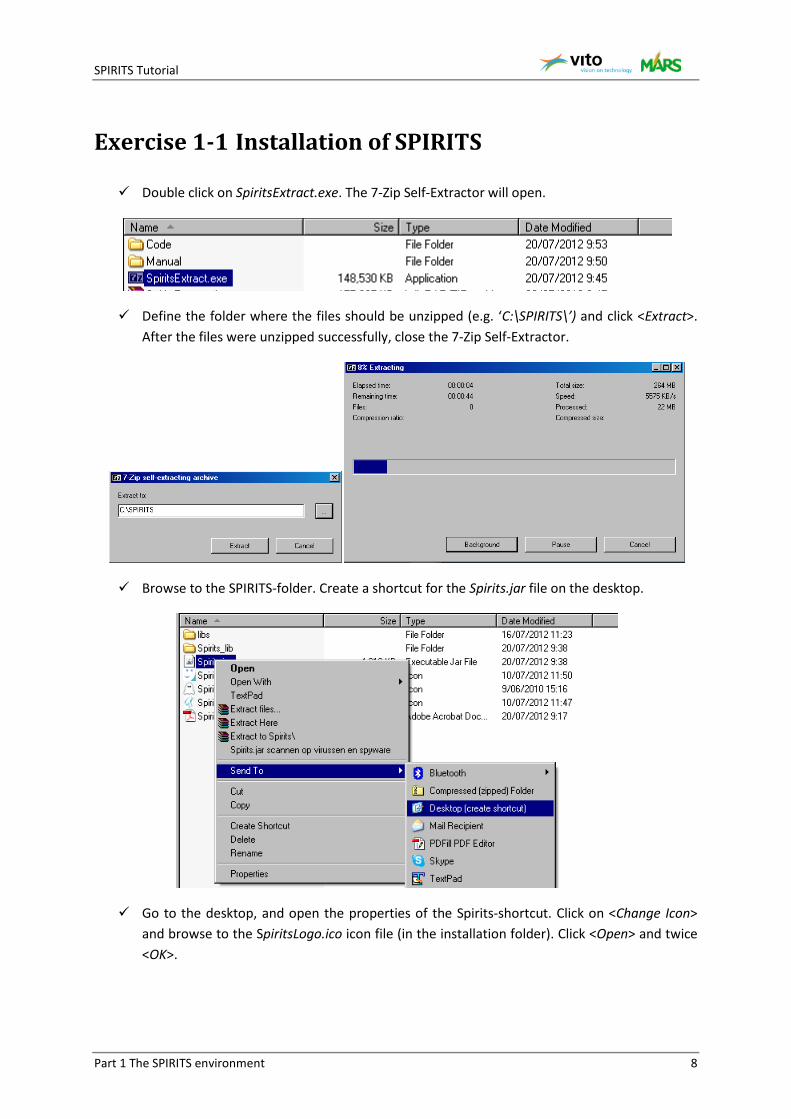
Double click on SpiritsExtract.exe. The 7-Zip Self-Extractor will open.

Define the folder where the files should be unzipped (e.g. ‘C:\SPIRITS\’) and click <Extract>. After the files were unzipped successfully, close the 7-Zip Self-Extractor.

Browse to the SPIRITS-folder. Create a shortcut for the Spirits.jar file on the desktop.

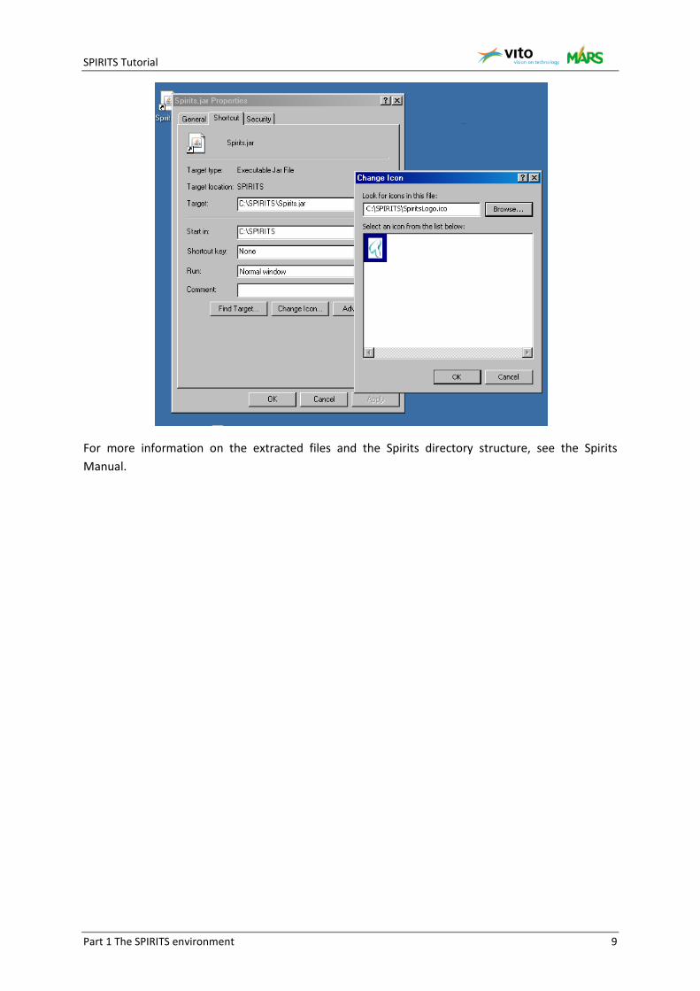
Go to the desktop, and open the properties of the Spirits-shortcut. Click on <Change Icon> and browse to the SpiritsLogo.ico icon file (in the installation folder). Click <Open> and twice <OK>.

SPIRITS Tutorial


For more information on the extracted files and the Spirits directory structure, see the Spirits Manual.

SPIRITS Tutorial


Exercise 1-2 Getting started

To start SPIRITS, double-click on the SPIRITS application icon on your desktop, or double-click on Spirits.jar in the installation folder.

WARNING: In order for SPIRITS to work properly, JAVA 1.6 needs to be installed on your computer.1

Now explore the SPIRITS main window.

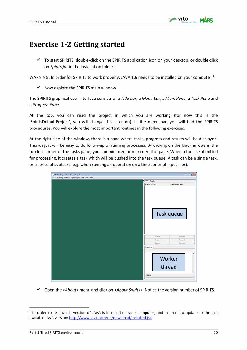
The SPIRITS graphical user interface consists of a Title bar, a Menu bar, a Main Pane, a Task Pane and a Progress Pane.

At the top, you can read the project in which you are working (for now this is the ‘SpiritsDefaultProject’, you will change this later on). In the menu bar, you will find the SPIRITS procedures. You will explore the most important routines in the following exercises.

At the right side of the window, there is a pane where tasks, progress and results will be displayed. This way, it will be easy to do follow-up of running processes. By clicking on the black arrows in the top left corner of the tasks pane, you can minimize or maximize this pane. When a tool is submitted for processing, it creates a task which will be pushed into the task queue. A task can be a single task, or a series of subtasks (e.g. when running an operation on a time series of input files).

Open the <About> menu and click on <About Spirits>. Notice the version number of SPIRITS.

1 In order to test which version of JAVA is installed on your computer, and in order to update to the last available JAVA version: http://www.java.com/en/download/installed.jsp.

Worker thread

Task queue

http://www.java.com/en/download/installed.jsp

SPIRITS Tutorial


Exercise 1-3 The SPIRITS TUTORIAL project

When you open SPIRITS for the first time, a default project is created, named SpiritsDefaultProject. The project refers to a directory with the same name in the installation folder: ‘.\Spirits\SpiritsDefaultProject\’.

For the tutorial, you will change the project name and project resource folders. The project concept offers the possibility to group related user data (images, tools, scenarios, templates for maps etc.) without demanding a fixed or predefined file system structure.

Download the TUTORIAL data and save the entire directory on your hard disk.

In the following sections, we will use the case where the tutorial data is stored in ‘D:\TUTORIAL\’ as example case, but you are free to save the TUTORIAL directory on another hard disk drive. Two important remarks:

• Be aware that you will generate lots of data in the following exercises, and that there needs to be at least 1.5 GB of free disk storage on the disk where you store the tutorial data.

• SPIRITS can show errors when data are stored in a directory with a very long path. Therefore consider saving the tutorial data directly on your hard disk (as was done in the example case), instead of copying it e.g. on your desktop.

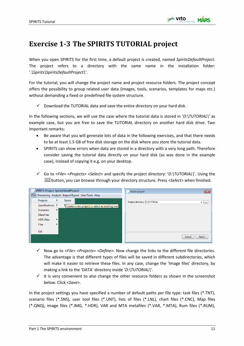
Go to <File> <Projects> <Select> and specify the project directory: ‘D:\TUTORIAL\’. Using the

button, you can browse through your directory structure. Press <Select> when finished.

Now go to <File> <Projects> <Define>. Now change the links to the different file directories. The advantage is that different types of files will be saved in different subdirectories, which will make it easier to retrieve these files. In any case, change the ‘Image files’ directory, by making a link to the ‘DATA’ directory inside ‘D:\TUTORIAL\’.

It is very convenient to also change the other resource folders as shown in the screenshot below. Click <Save>.

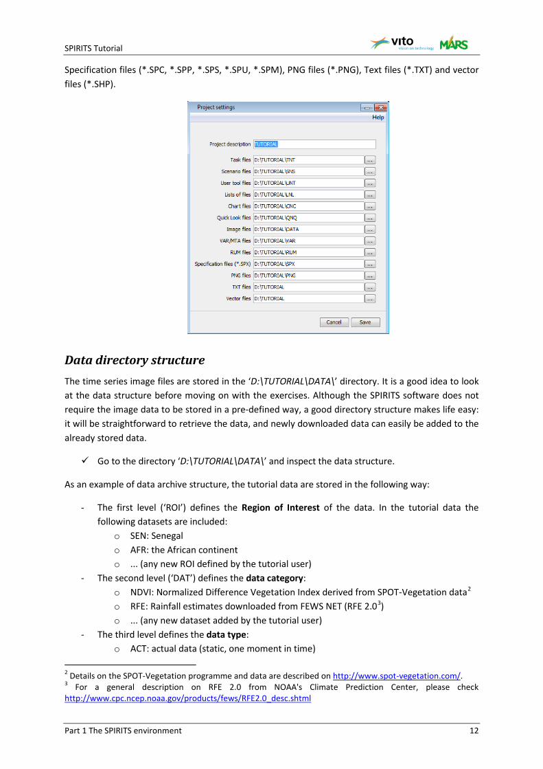
In the project settings you have specified a number of default paths per file type: task files (*.TNT), scenario files (*.SNS), user tool files (*.UNT), lists of files (*.LNL), chart files (*.CNC), Map files (*.QNQ), image files (*.IMG, *.HDR), VAR and MTA metafiles (*.VAR, *.MTA), Rum files (*.RUM),

SPIRITS Tutorial


Specification files (*.SPC, *.SPP, *.SPS, *.SPU, *.SPM), PNG files (*.PNG), Text files (*.TXT) and vector files (*.SHP).

Data directory structure The time series image files are stored in the ‘D:\TUTORIAL\DATA\’ directory. It is a good idea to look at the data structure before moving on with the exercises. Although the SPIRITS software does not require the image data to be stored in a pre-defined way, a good directory structure makes life easy: it will be straightforward to retrieve the data, and newly downloaded data can easily be added to the already stored data.

Go to the directory ‘D:\TUTORIAL\DATA\’ and inspect the data structure.

As an example of data archive structure, the tutorial data are stored in the following way:

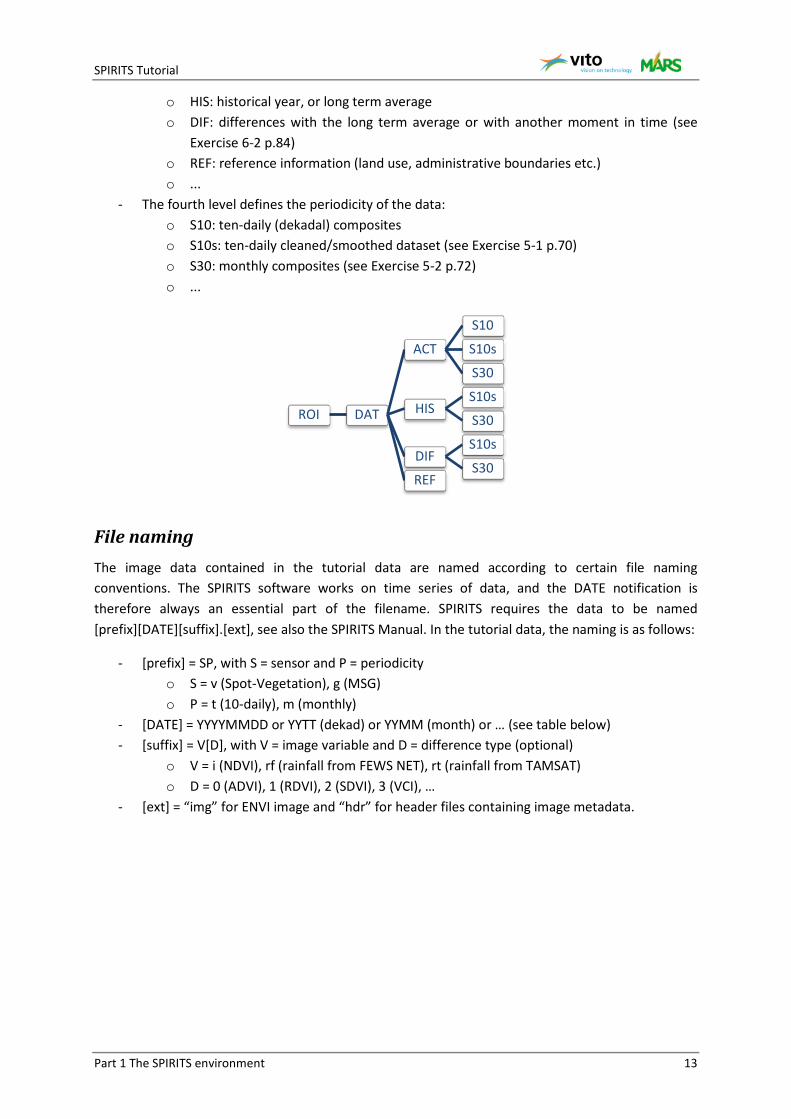
- The first level (‘ROI’) defines the Region of Interest of the data. In the tutorial data the following datasets are included:

o SEN: Senegal o AFR: the African continent o ... (any new ROI defined by the tutorial user)

- The second level (‘DAT’) defines the data category: o NDVI: Normalized Difference Vegetation Index derived from SPOT-Vegetation data2 o RFE: Rainfall estimates downloaded from FEWS NET (RFE 2.03) o ... (any new dataset added by the tutorial user)

- The third level defines the data type: o ACT: actual data (static, one moment in time)

2 Details on the SPOT-Vegetation programme and data are described on http://www.spot-vegetation.com/. 3 For a general description on RFE 2.0 from NOAA's Climate Prediction Center, please check http://www.cpc.ncep.noaa.gov/products/fews/RFE2.0_desc.shtml

http://www.spot-vegetation.com/

http://www.cpc.ncep.noaa.gov/products/fews/RFE2.0_desc.shtml

SPIRITS Tutorial


o HIS: historical year, or long term average o DIF: differences with the long term average or with another moment in time (see

Exercise 6-2 p.84) o REF: reference information (land use, administrative boundaries etc.) o ...

- The fourth level defines the periodicity of the data: o S10: ten-daily (dekadal) composites o S10s: ten-daily cleaned/smoothed dataset (see Exercise 5-1 p.70) o S30: monthly composites (see Exercise 5-2 p.72) o ...

File naming The image data contained in the tutorial data are named according to certain file naming conventions. The SPIRITS software works on time series of data, and the DATE notification is therefore always an essential part of the filename. SPIRITS requires the data to be named [prefix][DATE][suffix].[ext], see also the SPIRITS Manual. In the tutorial data, the naming is as follows:

- [prefix] = SP, with S = sensor and P = periodicity o S = v (Spot-Vegetation), g (MSG) o P = t (10-daily), m (monthly)

- [DATE] = YYYYMMDD or YYTT (dekad) or YYMM (month) or … (see table below) - [suffix] = V[D], with V = image variable and D = difference type (optional)

o V = i (NDVI), rf (rainfall from FEWS NET), rt (rainfall from TAMSAT) o D = 0 (ADVI), 1 (RDVI), 2 (SDVI), 3 (VCI), …

- [ext] = “img” for ENVI image and “hdr” for header files containing image metadata.

ROI DAT

ACT

S10

S10s

S30

HIS S10s

S30

DIF S10s

S30 REF

SPIRITS Tutorial


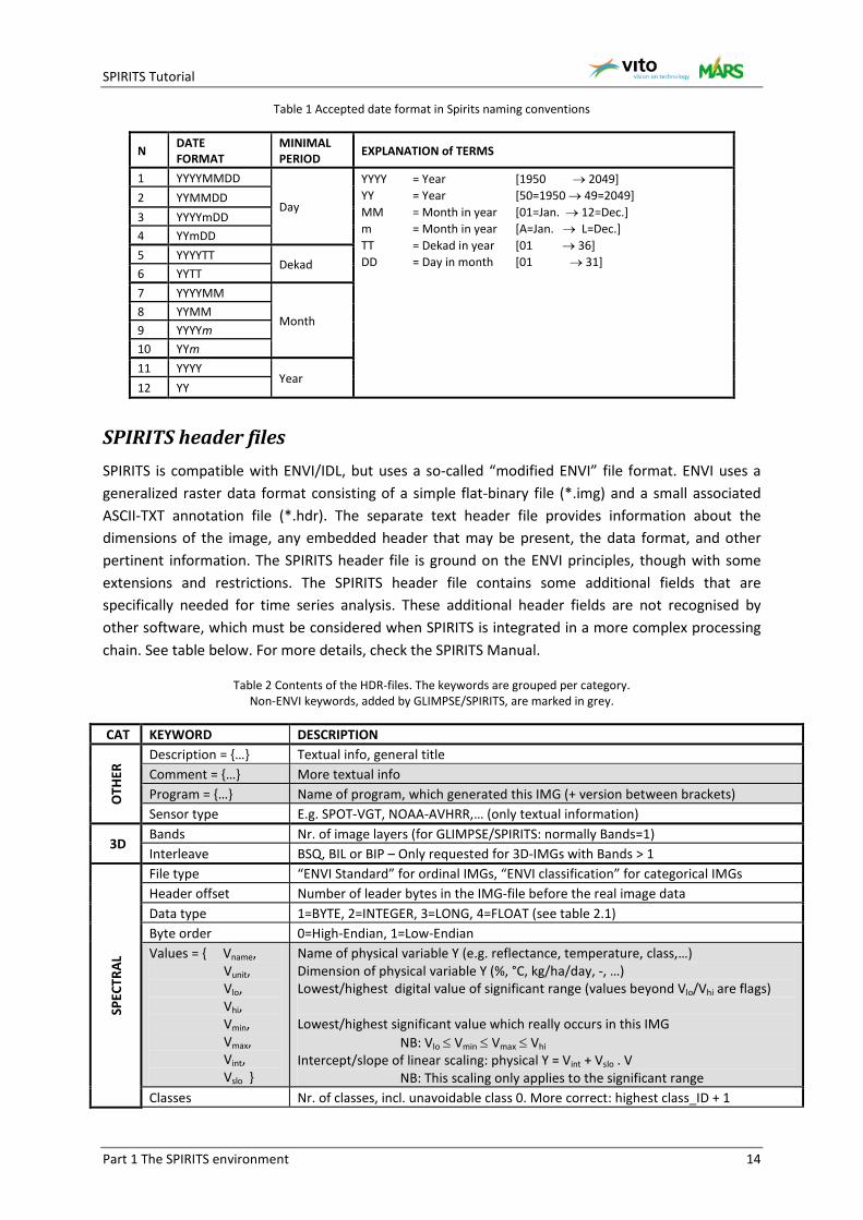
Table 1 Accepted date format in Spirits naming conventions

N DATE FORMAT

MINIMAL PERIOD EXPLANATION of TERMS

1 YYYYMMDD

Day

YYYY = Year [1950 → 2049] YY = Year [50=1950 → 49=2049] MM = Month in year [01=Jan. → 12=Dec.] m = Month in year [A=Jan. → L=Dec.] TT = Dekad in year [01 → 36] DD = Day in month [01 → 31]

2 YYMMDD 3 YYYYmDD 4 YYmDD 5 YYYYTT

Dekad 6 YYTT 7 YYYYMM

Month 8 YYMM 9 YYYYm 10 YYm 11 YYYY

Year 12 YY

SPIRITS header files SPIRITS is compatible with ENVI/IDL, but uses a so-called “modified ENVI” file format. ENVI uses a generalized raster data format consisting of a simple flat-binary file (*.img) and a small associated ASCII-TXT annotation file (*.hdr). The separate text header file provides information about the dimensions of the image, any embedded header that may be present, the data format, and other pertinent information. The SPIRITS header file is ground on the ENVI principles, though with some extensions and restrictions. The SPIRITS header file contains some additional fields that are specifically needed for time series analysis. These additional header fields are not recognised by other software, which must be considered when SPIRITS is integrated in a more complex processing chain. See table below. For more details, check the SPIRITS Manual.

Table 2 Contents of the HDR-files. The keywords are grouped per category. Non-ENVI keywords, added by GLIMPSE/SPIRITS, are marked in grey.

CAT KEYWORD DESCRIPTION

OTH

ER Description = {…} Textual info, general title

Comment = {…} More textual info Program = {…} Name of program, which generated this IMG (+ version between brackets) Sensor type E.g. SPOT-VGT, NOAA-AVHRR,… (only textual information)

3D Bands Nr. of image layers (for GLIMPSE/SPIRITS: normally Bands=1) Interleave BSQ, BIL or BIP – Only requested for 3D-IMGs with Bands > 1

SPEC

TRAL

File type “ENVI Standard” for ordinal IMGs, “ENVI classification” for categorical IMGs Header offset Number of leader bytes in the IMG-file before the real image data Data type 1=BYTE, 2=INTEGER, 3=LONG, 4=FLOAT (see table 2.1) Byte order 0=High-Endian, 1=Low-Endian Values = { Vname, Vunit, Vlo, Vhi, Vmin, Vmax, Vint, Vslo }

Name of physical variable Y (e.g. reflectance, temperature, class,…) Dimension of physical variable Y (%, °C, kg/ha/day, -, …) Lowest/highest digital value of significant range (values beyond Vlo/Vhi are flags) Lowest/highest significant value which really occurs in this IMG NB: Vlo ≤ Vmin ≤ Vmax ≤ Vhi Intercept/slope of linear scaling: physical Y = Vint + Vslo . V NB: This scaling only applies to the significant range

Classes Nr. of classes, incl. unavoidable class 0. More correct: highest class_ID + 1

SPIRITS Tutorial


Class names = {…} For each class, starting with 0: class name (avoid commas!) Class lookup = {…} For each class, starting with 0: R, G, B-values in range 0-255 Flags = {…} For each flag: “V=meaning” with V=digital value (only textual info!)

SPAT

IAL

Samples Number of IMG columns (Ncol) Lines Number of IMG records or lines (Nrec) Map info = { Name ,Colm, Recm ,Xm, Ym ,∆X, ∆Y [,zone, N/S] [,datum] [,units=x] }

Projection_Name (must be entry in ENVI file Map_proj.txt) IMG Col/Rec co-ordinates of “Magic Point” (see figure 2.3) Map X/Y co-ordinates of same “Magic Point” X/Y pixel size in map-units Only for Projection_name=UTM: zone [1-60] and “North” or “South” Optional: geodetic datum (entry ENVI-file Datum.txt) map units: x=“Metres” or “Degrees”

Projection info = {...} All specifications of map projection. Same form as used in ENVI-file Map_proj.txt.

TMP Date YYYYMMDD: IMG registration date, or start date for composite IMGs Days Periodicity in days: 1, 10, 30,…; 0=unknown/irrelevant; -1=actual registration

SPIRITS Tutorial

Part 2 Quick start 16

Part 2 Quick start

This section includes a first exercises in order to offer a first glimpse on the power of SPIRITS when it comes to time series processing: first you will make a map (also called Map or image preview) of one single image using a predefined template, then this template will be used to automatically create a set of maps over a time series to see the temporal evolution of a variable.

After this first exercise, a number of good practices are discussed.

! Reference to exercise data is done by default to a folder called ‘D:\TUTORIAL\DATA\’. If you have installed the tutorial dataset on your C-drive, use the ‘Senegal_NDVI_C.qnq’ template in the example below.

Using a map template First, you will visualize a map of an NDVI image:

Open the <Create template> tool in <Analysis> <Maps>. Click <File> <Open> and load the pre-fabricated Map template for Senegal (named

‘Senegal_NDVI.qnq’), which you will find in the ‘D:\TUTORIAL\QNQ’ directory.

Note that you have loaded a Normalized Difference Vegetation Index image (TOC: top of canopy) derived from the SPOT-Vegetation satellite. This map gives an idea on the status of vegetation cover in Senegal over the first dekad (10 day period) of January 2012.

SPIRITS Tutorial


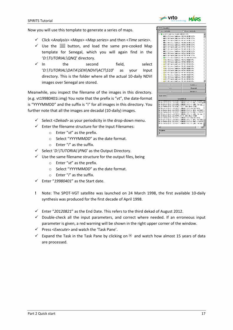
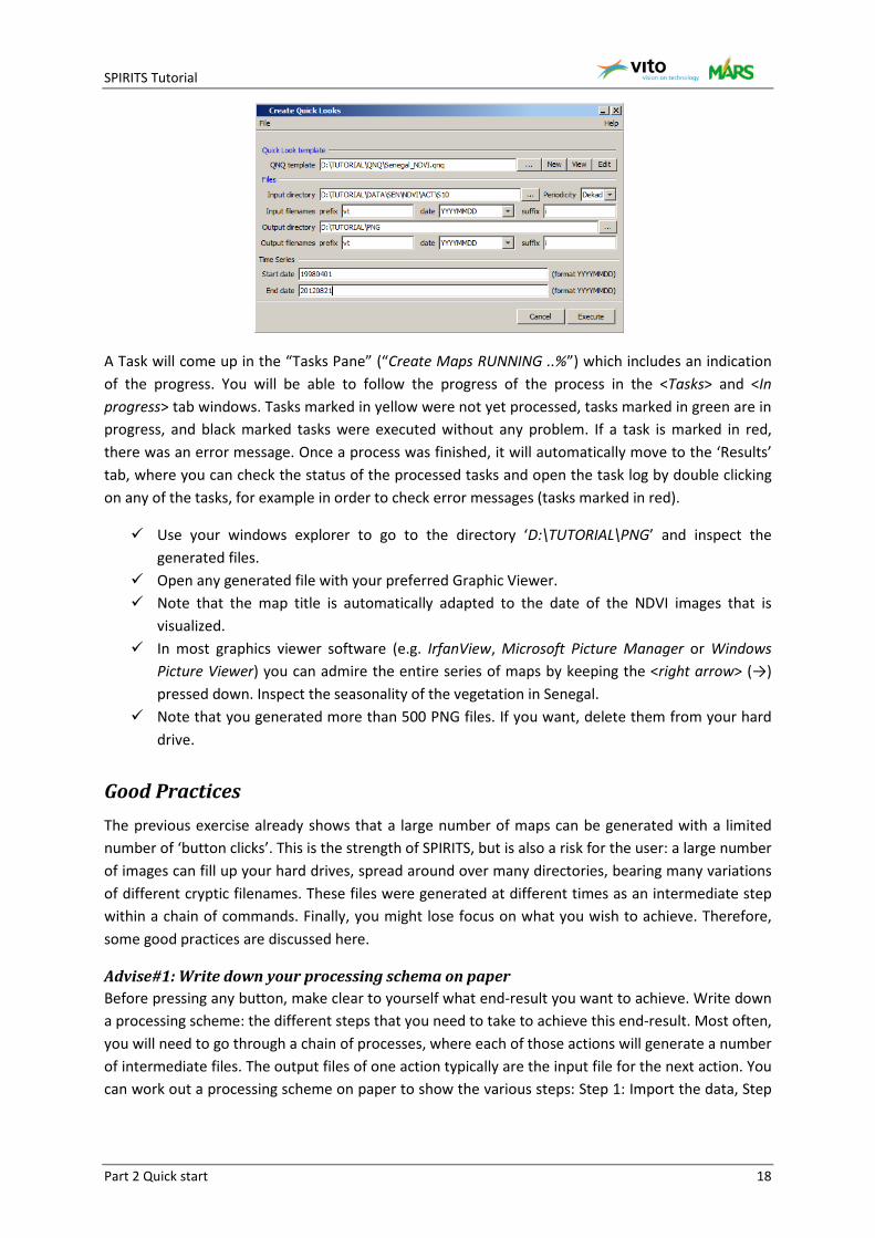
Now you will use this template to generate a series of maps.

Click <Analysis> <Maps> <Map series> and then <Time series>. Use the button, and load the same pre-cooked Map

template for Senegal, which you will again find in the ‘D:\TUTORIAL\QNQ’ directory.

In the second field, select ‘D:\TUTORIAL\DATA\SEN\NDVI\ACT\S10’ as your Input directory. This is the folder where all the actual 10-daily NDVI images over Senegal are stored.

Meanwhile, you inspect the filename of the images in this directory. (e.g. vt19980401i.img) You note that the prefix is ”vt”, the date-format is “YYYYMMDD” and the suffix is “i” for all images in this directory. You further note that all the images are decadal (10-daily) images.

Select <Dekad> as your periodicity in the drop-down menu. Enter the filename structure for the Input Filenames:

o Enter “vt” as the prefix. o Select “YYYYMMDD” as the date format. o Enter “i” as the suffix.

Select ‘D:\TUTORIAL\PNG’ as the Output Directory. Use the same filename structure for the output files, being

o Enter “vt” as the prefix. o Select “YYYYMMDD” as the date format. o Enter “i” as the suffix.

Enter “19980401” as the Start date.

! Note: The SPOT-VGT satellite was launched on 24 March 1998, the first available 10-daily synthesis was produced for the first decade of April 1998.

Enter “20120821” as the End Date. This refers to the third dekad of August 2012. Double-check all the input parameters, and correct where needed. If an erroneous input

parameter is given, a red warning will be shown in the right upper corner of the window. Press <Execute> and watch the ‘Task Pane’. Expand the Task in the Task Pane by clicking on and watch how almost 15 years of data

are processed.

SPIRITS Tutorial


A Task will come up in the “Tasks Pane” (“Create Maps RUNNING ..%”) which includes an indication of the progress. You will be able to follow the progress of the process in the <Tasks> and <In progress> tab windows. Tasks marked in yellow were not yet processed, tasks marked in green are in progress, and black marked tasks were executed without any problem. If a task is marked in red, there was an error message. Once a process was finished, it will automatically move to the ‘Results’ tab, where you can check the status of the processed tasks and open the task log by double clicking on any of the tasks, for example in order to check error messages (tasks marked in red).

Use your windows explorer to go to the directory ‘D:\TUTORIAL\PNG’ and inspect the generated files.

Open any generated file with your preferred Graphic Viewer. Note that the map title is automatically adapted to the date of the NDVI images that is

visualized. In most graphics viewer software (e.g. IrfanView, Microsoft Picture Manager or Windows

Picture Viewer) you can admire the entire series of maps by keeping the <right arrow> (→) pressed down. Inspect the seasonality of the vegetation in Senegal.

Note that you generated more than 500 PNG files. If you want, delete them from your hard drive.

Good Practices The previous exercise already shows that a large number of maps can be generated with a limited number of ‘button clicks’. This is the strength of SPIRITS, but is also a risk for the user: a large number of images can fill up your hard drives, spread around over many directories, bearing many variations of different cryptic filenames. These files were generated at different times as an intermediate step within a chain of commands. Finally, you might lose focus on what you wish to achieve. Therefore, some good practices are discussed here.

Advise#1: Write down your processing schema on paper Before pressing any button, make clear to yourself what end-result you want to achieve. Write down a processing scheme: the different steps that you need to take to achieve this end-result. Most often, you will need to go through a chain of processes, where each of those actions will generate a number of intermediate files. The output files of one action typically are the input file for the next action. You can work out a processing scheme on paper to show the various steps: Step 1: Import the data, Step

SPIRITS Tutorial


2: Generate maps to check the imported data, Step 3: Calculate the long term average,... etc. Some results of workflows are given in Part 8 Workflow examples (p.114)

Advise#2: Use a meaningful directory structure Make a clear and logic file directory structure with meaningful directory names,. It is a good idea to put new series of files in a new (sub)directory. The names of the directory should give you an idea about it contents. Intermediate or temporary files can be generated in temporarily sub-directories. The tutorial data are an example of an elaborated directory structure. Another example of a simple directory structure is:

• D:\PROJECT o DATA

01_import 02_quicklooks 03_lta 04_... Etc.

Advise#3: Stick to one filename convention The SPIRITS software works on time series of data, uses a fixed filename convention: the DATE notification is always an essential part of the filename. SPIRITS requires the data to be named [prefix][DATE][suffix].[ext], see also the SPIRITS Manual.

In the exercises, the following filename conventions are used:

- [prefix] = SP, with S = sensor and P = periodicity o S = v (Spot-Vegetation), e (Envisat-MERIS), g (MSG), a (NOAA-AVHRR), … o P = t (10-daily), m (monthly)

- [DATE] = YYYMMDD - [suffix] = V[D], with V = image variable and D = difference type (optional)

o V = i (NDVI), rf (rainfall from FEWS NET), rt (rainfall from TAMSAT) o D = 0 (ADVI), 1 (RDVI), 2 (SDVI), 3 (VCI), …

- [ext] = “img” for ENVI image and “hdr” for header files containing image metadata.

However, you are free to develop your own convention, as long as you stick to the general [prefix][DATE][suffix].[ext] structure. The filename should always be descriptive and give you the right information about the contents of the file.

Advise#4: First test the procedure on a single file In general, it is a good practice to first experiment your SPIRITS procedure (or task) on a single file or a limited range of the time series. After checking the content and the filename of the generated file, you can run a scenario for a large set of input files. A SPIRITS scenario is made when the same procedure needs to be ran over a time series of input files. The scenario is therefore a set of parameters for a specific function working on a time series.

Advise#5: Double-check all the parameters before hitting the <Execute> button It is important to check the parameters before hitting the <Execute> button. One press on an <Execute> button can have serious consequences if parameters are not correct. You can overwrite

SPIRITS Tutorial


important files (without warning!), or you can start a procedure with wrong parameters or which take long to finish.

Advise#6: Check your available disk space It is important to regularly check the available hard disk space. When generating a huge amount of files, your hard disc can easily silt. The processes will slow down, eventually leading in errors in your application. When you use a smart directory structure, you should be able to easily distinguish intermediate files from your crucial input/output files. It is wise to regularly clean up temporary or unnecessary files.

Advise#7: Check for errors After each step, it is a good practice to systematically check for errors the tasks in the <Tasks> and <Results> pane. All tasks which contained errors will be marked with a red bullet, tasks which executed correct have a black bullet. By clicking on the error-tasks, you can examine the log (including error description) in the <Progress> pane.

Advise#8: Check the contents of your results with your preferred GIS tool. Also when SPIRITS runs a process without error messages, the content of generated files can be erroneous. Therefore, after each operation, check the contents of the generated file(s) by using the map generator functionality of SPIRITS or by opening the file with your preferred GIS or image processing software. Note that scaling parameters (see the ‘values’ field in the image HDR) nor flags are recognized by other software that SPIRITS.

Advise#9: Think about the WHAT and the WHY of your actions. It is important to know what you are doing and why you are doing something. Also when doing the exercises in this tutorial, do not follow the instructions blindly but try to realize why the steps are performed in the way they are presented.

SPIRITS Tutorial

21

Part 3 Map generation

In this part you will learn how to use the SPIRITS map generator for the display of SPIRITS images. This section consists of 2 exercises, each containing a number of subsections:

• Exercise 3-1 Map templates and visualizing one image including maps of NDVI images, rainfall estimates, land cover maps, vegetation anomalies and rainfall anomalies

• Exercise 3-2 Generation of map series including map series NDVI, RFE, vegetation anomalies and rainfall anomalies

In the first exercise, you will learn how to use the map generator for the visualization of images (IMG) and vector layers (Shapefiles), and how to add a legend, title, logo, etc. Once a map template is finalized and saved as a Map template (*.qnq) file, the template can be used to generate series of maps, as is shown in the second exercise.

! Reference to exercise data is done by default to a folder called ‘D:\TUTORIAL\DATA\’.

SPIRITS Tutorial

22

Exercise 3-1 Map templates and visualizing one image

The map generator enables the visualization of images (IMG) and vector layers (Shapefiles), and allows the user to add a legend, title, logo, etc. Note that the SPIRITS map generator is not a GIS interface, you can therefore not zoom nor query the values of the image.

Once a Map template is finalized and saved as a *.qnq file, the template can be used to generate map series, see Exercise 3-2 Generation of map series (p.31).

Map template of NDVI images over Senegal First, you will make a map of an NDVI image. Now you will not start from the pre-generated Map template, but design your own.

Start up the <Create template> window from <Analysis> <Maps>.

At the top of the Map generator window, you can either visualize the map, or the HDR file associated with a loaded image. At the bottom of the window, you can change all aspects of the Map.

First you load an image to the map, and you change its size and position.

In the <Image> tab, click on and load an image, for example one of the actual 10-daily NDVI images for Senegal in ‘D:\TUTORIAL\DATA\SEN\NDVI\ACT\S10\’. The image is displayed in gray.

SPIRITS Tutorial

23

Change the image position and size so it is placed in the upper left corner (e.g. Left = “30”, Top = “30”, Height = “320” pixels). The value of the Width field will automatically be adapted to maintain the same ratio between Height and Width.

Change the Border Width to “1” and Border Margin to “0”.

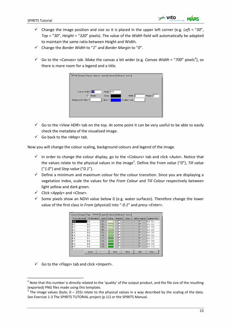
Go to the <Canvas> tab. Make the canvas a bit wider (e.g. Canvas Width = “700” pixels4), so there is more room for a legend and a title.

Go to the <View HDR> tab on the top. At some point it can be very useful to be able to easily check the metadata of the visualized image.

Go back to the <Map> tab.

Now you will change the colour scaling, background colours and legend of the image.

In order to change the colour display, go to the <Colours> tab and click <Auto>. Notice that the values relate to the physical values in the image5. Define the From value (“0”), Till value (“1.0”) and Step value (“0.1”).

Define a minimum and maximum colour for the colour transition. Since you are displaying a vegetation index, scale the values for the From Colour and Till Colour respectively between light yellow and dark green.

Click <Apply> and <Close>. Some pixels show an NDVI value below 0 (e.g. water surfaces). Therefore change the lower

value of the first class in From (physical) into “-0.1” and press <Enter>.

Go to the <Flags> tab and click <Import>.

4 Note that this number is directly related to the ‘quality’ of the output product, and the file size of the resulting (exported) PNG files made using this template. 5 The image values (byte, 0 – 255) relate to the physical values in a way described by the scaling of the data. See Exercise 1-3 The SPIRITS TUTORIAL project (p.11) or the SPIRITS Manual.

SPIRITS Tutorial

24

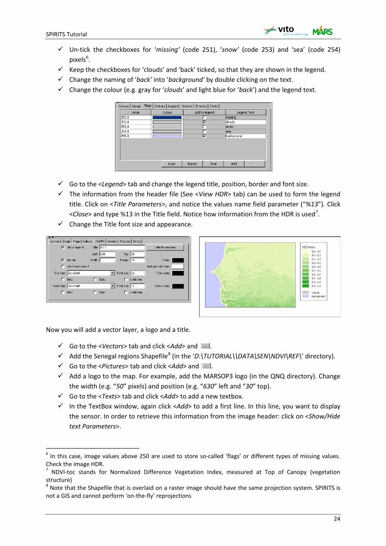
Un-tick the checkboxes for ‘missing’ (code 251), ‘snow’ (code 253) and ‘sea’ (code 254) pixels6.

Keep the checkboxes for ‘clouds’ and ‘back’ ticked, so that they are shown in the legend. Change the naming of ‘back’ into ‘background’ by double clicking on the text. Change the colour (e.g. gray for ‘clouds’ and light blue for ‘back’) and the legend text.

Go to the <Legend> tab and change the legend title, position, border and font size. The information from the header file (See <View HDR> tab) can be used to form the legend

title. Click on <Title Parameters>, and notice the values name field parameter (“%13”). Click <Close> and type %13 in the Title field. Notice how information from the HDR is used7.

Change the Title font size and appearance.

Now you will add a vector layer, a logo and a title.

Go to the <Vectors> tab and click <Add> and . Add the Senegal regions Shapefile8 (in the ‘D:\TUTORIAL\\DATA\SEN\NDVI\REF\’ directory). Go to the <Pictures> tab and click <Add> and . Add a logo to the map. For example, add the MARSOP3 logo (in the QNQ directory). Change

the width (e.g. “50” pixels) and position (e.g. “630” left and “30” top). Go to the <Texts> tab and click <Add> to add a new textbox. In the TextBox window, again click <Add> to add a first line. In this line, you want to display

the sensor. In order to retrieve this information from the image header: click on <Show/Hide text Parameters>.

6 In this case, image values above 250 are used to store so-called ‘flags’ or different types of missing values. Check the image HDR. 7 NDVI-toc stands for Normalized Difference Vegetation Index, measured at Top of Canopy (vegetation structure) 8 Note that the Shapefile that is overlaid on a raster image should have the same projection system. SPIRITS is not a GIS and cannot perform ‘on-the-fly’ reprojections

SPIRITS Tutorial

25

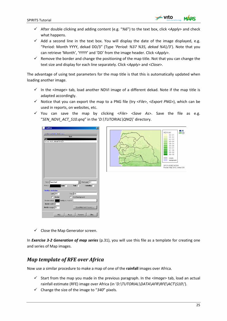
After double clicking and adding content (e.g. “%6”) to the text box, click <Apply> and check what happens.

Add a second line in the text box. You will display the date of the image displayed, e.g. “Period: Month YYYY, dekad DD/3” (Type ‘Period: %37 %35, dekad %41/3’). Note that you can retrieve ‘Month’, ‘YYYY’ and ‘DD’ from the image header. Click <Apply>.

Remove the border and change the positioning of the map title. Not that you can change the text size and display for each line separately. Click <Apply> and <Close>.

The advantage of using text parameters for the map title is that this is automatically updated when loading another image.

In the <Image> tab, load another NDVI image of a different dekad. Note if the map title is adapted accordingly.

Notice that you can export the map to a PNG file (try <File>, <Export PNG>), which can be used in reports, on websites, etc.

You can save the map by clicking <File> <Save As>. Save the file as e.g. “SEN_NDVI_ACT_S10.qnq” in the ‘D:\TUTORIAL\QNQ\’ directory.

Close the Map Generator screen.

In Exercise 3-2 Generation of map series (p.31), you will use this file as a template for creating one and series of Map images.

Map template of RFE over Africa Now use a similar procedure to make a map of one of the rainfall images over Africa.

Start from the map you made in the previous paragraph. In the <Image> tab, load an actual rainfall estimate (RFE) image over Africa (in ‘D:\TUTORIAL\DATA\AFR\RFE\ACT\S10\’).

Change the size of the image to “340” pixels.

SPIRITS Tutorial

26

Change the width of the canvas size to “600”. Move the position of the legend, title and logo 100 pixels to the left. Edit the colour scale: click on <Auto>, choose a 3 colour transition, and for example define

the ‘from’, ‘reference’, ‘till’ and ‘step’ value as “0”, “150”, “250” and “50” respectively. Note that these values relate to cumulative mm of rainfall over the dekad.

Choose the ‘Gradients’ colour type and define the ‘From Colour’, ‘Reference Colour’ and ‘Till Colour’ as white, dark blue and purple respectively.

Click <Apply> and close the ‘Auto create colours’ window. Remove the vector file with the Senegalese regions9, and replace it with the Shapefile with

the borders of the African countries (in ‘D:\TUTORIAL\DATA\AFR\RFE\REF\’) Note that the flags should not be displayed in the legend. In the ‘Flags’ tab, uncheck the ‘Add

to legend’ boxes. Note that the map title should display the source of the rainfall estimates data. Go to the

‘Texts’ tab, select the entry, click <Edit> and change the first line of the text box. Use the ‘description’ header (HDR) parameter instead of the ‘sensor type’ parameter. Close the TextBox window.

Save the Map as “AFR_RFE_ACT_S10.qnq” so you can use the template later on.

The created Map template window looks like the example below.

Load several rainfall images and evaluate the rainfall on several periods of the year and check whether the title entry changes correctly.

9 The reason why this Shapefile is not visible on the RFE image, is because the projection system of the RFE image (Albers Equal Area Conic) is different from the SPOT-Vegetation NDVI and regions Shapefile we used before (Geographical Lat/Lon)

SPIRITS Tutorial

27

Close the Map Generator screen.

Map template of RFE over Senegal This exercise can only be performed after finalizing Exercise 4-2 Extract ROI (p.50). In this example you can use a similar procedure to make a map of one of the rainfall images over Senegal.

Start from the Map you made for visualizing RFE images over Africa (<File> <Open> and select ‘AFR_RFE_ACT_S10.qnq’).

In the <Image> tab, load an actual rainfall estimate (RFE) image over Senegal (in ‘D:\TUTORIAL\DATA\SEN\RFE\ACT\S10\’).

In the <Vectors> tab, change the vector file with the regions Shapefile located in ‘D:\TUTORIAL\DATA\SEN\RFE\REF\’.

In the <Texts> tab, change the text box position in “280” from the top. In the <Canvas> tab, change the Canvas Height in “360”. Save the Map as “AFR_RFE_ACT_S10.qnq” so you can use the template later on.

Map of a land cover map Now you will make a map of the GLC200010 land cover map over Africa. The file you will use for display is a so-called ENVI Classification file, with class names and class colours defined in the image HDR file.

Start from the map you made in the previous paragraph. In the <Image> tab, load the glc2000.img over Africa (in ‘D:\TUTORIAL\DATA\AFR\RFE\REF\’).

In this example, you will use the colour template as it is defined in the HDR file of the land cover map. Go to the <Colours> tab, and click on <Import>.

Visualize the HDR by opening the <View HDR> tab. Note how the colours (class lookup) and the legend entries (class names) are automatically adapted according to the entries in the image HDR file.

Return to the <Map> tab. Note that some adaptations are necessary in order for the legend to be displayed entirely.

10 Mayaux, P., Bartholomé, E., Massart, M., Van Cutsem, C., Cabral, A., Nonguierma, A., Diallo, O., Pretorius, C., Thompson, M., Cherlet, M., Pekel, J.-F., Defourny, P., Vasconcelos, M., Di Gregorio, A., Fritz, S., De Grandi, G., Elvidge, C., Vogt, P., Belward, A., 2003. A land cover map of Africa, European Commission - JRC.

SPIRITS Tutorial

28

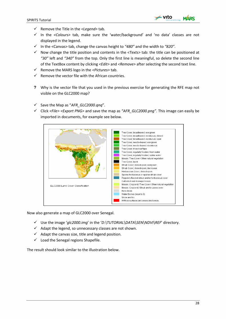
Remove the Title in the <Legend> tab. In the <Colours> tab, make sure the ‘water/background’ and ‘no data’ classes are not

displayed in the legend. In the <Canvas> tab, change the canvas height to “480” and the width to “820”. Now change the title position and contents in the <Texts> tab: the title can be positioned at

“30” left and “340” from the top. Only the first line is meaningful, so delete the second line of the TextBox content by clicking <Edit> and <Remove> after selecting the second text line.

Remove the MARS logo in the <Pictures> tab. Remove the vector file with the African countries.

? Why is the vector file that you used in the previous exercise for generating the RFE map not

visible on the GLC2000 map?

Save the Map as “AFR_GLC2000.qnq”. Click <File> <Export PNG> and save the map as “AFR_GLC2000.png”. This image can easily be

imported in documents, for example see below.

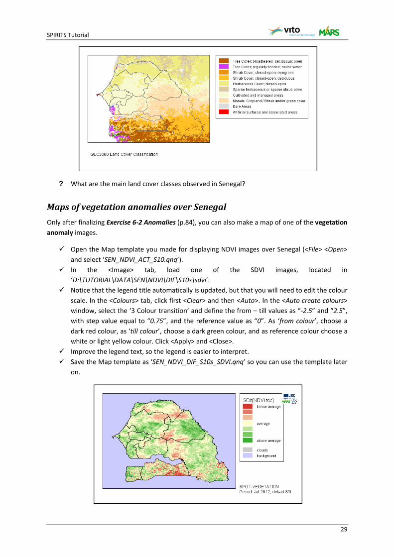
Now also generate a map of GLC2000 over Senegal.

Use the image ‘glc2000.img’ in the ‘D:\TUTORIAL\DATA\SEN\NDVI\REF’ directory. Adapt the legend, so unnecessary classes are not shown. Adapt the canvas size, title and legend position. Load the Senegal regions Shapefile.

The result should look similar to the illustration below.

SPIRITS Tutorial

29

? What are the main land cover classes observed in Senegal?

Maps of vegetation anomalies over Senegal Only after finalizing Exercise 6-2 Anomalies (p.84), you can also make a map of one of the vegetation anomaly images.

Open the Map template you made for displaying NDVI images over Senegal (<File> <Open> and select ‘SEN_NDVI_ACT_S10.qnq’).

In the <Image> tab, load one of the SDVI images, located in ‘D:\TUTORIAL\DATA\SEN\NDVI\DIF\S10s\sdvi’.

Notice that the legend title automatically is updated, but that you will need to edit the colour scale. In the <Colours> tab, click first <Clear> and then <Auto>. In the <Auto create colours> window, select the ‘3 Colour transition’ and define the from – till values as “-2.5” and “2.5”, with step value equal to “0.75”, and the reference value as “0”. As ‘from colour’, choose a dark red colour, as ‘till colour’, choose a dark green colour, and as reference colour choose a white or light yellow colour. Click <Apply> and <Close>.

Improve the legend text, so the legend is easier to interpret. Save the Map template as ‘SEN_NDVI_DIF_S10s_SDVI.qnq’ so you can use the template later

on.

SPIRITS Tutorial

30

? Load several SDVI images. Which dekads have a particular good or bad vegetation status compared to the long term average?

Map of rainfall anomalies over Senegal After finalizing Exercise 6-2 Anomalies (p.84), you can also make a map of one of the rainfall anomaly images.

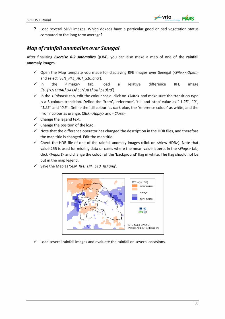
Open the Map template you made for displaying RFE images over Senegal (<File> <Open> and select ‘SEN_RFE_ACT_S10.qnq’).

In the <Image> tab, load a relative difference RFE image (‘D:\TUTORIAL\DATA\SEN\RFE\DIF\S10\rd’).

In the <Colours> tab, edit the colour scale: click on <Auto> and make sure the transition type is a 3 colours transition. Define the ‘from’, ‘reference’, ‘till’ and ‘step’ value as “-1.25”, “0”, “1.25” and “0.5”. Define the ‘till colour’ as dark blue, the ‘reference colour’ as white, and the ‘from’ colour as orange. Click <Apply> and <Close>.

Change the legend text. Change the position of the logo. Note that the difference operator has changed the description in the HDR files, and therefore

the map title is changed. Edit the map title. Check the HDR file of one of the rainfall anomaly images (click on <View HDR>). Note that

value 255 is used for missing data or cases where the mean value is zero. In the <Flags> tab, click <Import> and change the colour of the ‘background’ flag in white. The flag should not be put in the map legend.

Save the Map as ‘SEN_RFE_DIF_S10_RD.qnq’.

Load several rainfall images and evaluate the rainfall on several occasions.

SPIRITS Tutorial

Part 3 Map generation 31

Exercise 3-2 Generation of map series

Generating map series of NDVI over SENEGAL Go to <Analysis> <Maps> <Map series> <Time series>. Use the button, and load the Map template for Senegal that you created in Exercise 3-1

called “SEN_NDVI_ACT_S10.qnq” and stored in the ‘D:\TUTORIAL\QNQ\’ directory. In the second field, select ‘D:\TUTORIAL\DATA\SEN\NDVI\ACT\S10’ as your Input directory.

This is the folder where all the actual 10-daily NDVI images over Senegal are stored. Meanwhile, you inspect the filename of the images in this directory (e.g. vt19980401i.img).

Select <Dekad> as your periodicity in the drop-down menu. o Enter the filename structure for the Input Filenames: “vt” as the prefix,

“YYYYMMDD” as the date format and “i” as the suffix. Select ‘D:\TUTORIAL\PNG\SEN_QLK_NDVI_ACT_S10’ as the Output Directory (you will have

to create a new subdirectory in the PNG directory). o Use the same filename structure for the output files, being “vt” as the prefix,

“YYYYMMDD” as the date format and “i” as the suffix. Enter a start and end date (e.g. 20110401 till now) Press <Execute> and watch the “Task Pane”. Expand the Task in the Task Pane by clicking on and watch how data are processed.

A Task will come up in the “Tasks Pane” (“Create Maps RUNNING ..%”) which includes an indication of the progress. You will be able to follow the progress of the process in the <Tasks> and <In progress> tab windows. Tasks marked in yellow were not yet processed, tasks marked in green are in progress, and black marked tasks were executed without any problem. If a task is marked in red, there was an error message. Once a process was finished, it will automatically move to the ‘Results’ tab, where you can check the status of the processed tasks and open the task log by double clicking on any of the tasks, for example in order to check error messages (tasks marked in red).

Use your windows explorer to go to the directory ‘D:\TUTORIAL\PNG\SEN_QLK_NDVI_ACT_S10’ and inspect the generated files.

Open any generated file with your preferred Graphic Viewer.

SPIRITS Tutorial

Part 3 Map generation 32

Note that the map title is automatically adapted to the date of the NDVI images that is visualized.

In most graphics viewer software (e.g. IrfanView, Microsoft Picture Manager or Windows Picture Viewer) you can admire the entire series of maps by keeping the <right arrow> (→) pressed down. Inspect the seasonality of the vegetation in Senegal.

? In which decade of the year, the vegetation in Senegal is at maximum growth?

Generating map series for RFE over Senegal Use a similar procedure to generate a series of maps of RFE over Senegal (e.g. 20110401 till

now), using the Map template ‘SEN_RFE_ACT_S10.qnq’. Save the maps “gtYYYYMMDDrf.png” in ‘D:\TUTORIAL\PNG\SEN_QLK_RFE_ACT_S10’. Visualize the generated files.

? What is, in general, the start and end period of the rainy season in Senegal?

Generating map series of vegetation anomalies After finalizing Exercise 6-2 Anomalies (p.84) and creation of a Map template for displaying vegetation anomalies, you can also make a map series of the vegetation anomaly images.

Use a similar procedure to generate a series of maps of vegetation status anomalies over Senegal (e.g. 20110401 till now), using the Map template ‘SEN_NDVI_DIF_S10s_SDVI.qnq’.

Save the maps “vtYYYYMMDDk2.png” in ‘D:\TUTORIAL\PNG\ SEN_QLK_NDVI_DIF_S10s_SDVI’.

Visualize the generated files.

? In which dekads do you notice a clear lower vegetation status, compared to the average situation?

Generating map series of rainfall anomalies After finalizing Exercise 6-2 Anomalies (p.84) and creation of a Map template for displaying rainfall anomalies, you can also make map series of the rainfall anomaly images.

Use a similar procedure to generate a series of maps of RFE anomalies over Senegal (e.g. 20110401 till now), using the Map template ‘SEN_RFE_DIF_S10_RD.qnq’.

Save the maps “gtYYYYMMDDrf.png” in ‘D:\TUTORIAL\PNG\SEN_QLK_RFE_ACT_S10’. Go to the directory ‘D:\TUTORIAL\PNG\SEN_QLK_RFE_ACT_S10’ and inspect the generated

files.

? How would you describe rainfall over Senegal in July/2012, compared to the average situation?

SPIRITS Tutorial

Part 4 Basic SPIRITS routines 33

Part 4 Basic SPIRITS routines

This part contains exercises on a series of basic SPIRITS routines:

• Exercise 4-1 Import files including exercises on renaming and importing different file types, such as HDF, WinDisp or NetCDF files

• Exercise 4-2 Extract ROI including an exercise on the extraction of RFE over Senegal starting from RFE over Africa

• Exercise 4-3 Thinning including exercises on thinning of a classification image and an NDVI image

• Exercise 4-4 Area Fraction Images including an exercise on the generation of AFIs based on GlobCover

• Exercise 4-5 Image reclassification and scaling including exercises on reclassification of an NDVI image and scaling integer values to byte values

• Exercise 4-6 Rasterize Shapefiles including an exercise on the rasterize operation of Senegal regions from Shapefile to IMG

• Exercise 4-7 Masking including an exercise on the masking of S10 NDVI composites to S10m

• Exercise 4-8 Filtering including an exercise on the spatial filtering of S10 NDVI composites to S10f

• Exercise 4-9 Export files including an exercise on the export of time series to ENVI and the visualization of pixel profiles


SPIRITS Tutorial


Exercise 4-1 Import files

In many cases you will need to import files in order to generate ENVI IMG and HDR files starting from other file formats. Also when you want to use regular ENVI IMG files, some adaptations to the image HDR are necessary, in order to include the additional fields necessary for SPIRITS processing (see above).

In the different components of this exercise you will learn how to import single files or time series such as:

- WinDisp (rainfall estimates) from FEWS NET - NetCDF (rainfall estimates) from TAMSAT - HDF files (SPOT-Vegetation S10 NDVI) from DevCoCast

Importing WinDisp rainfall estimates from FEWS NET In this exercise we will show you how to import a time series of images in WinDisp format into SPIRITS. You will focus on the procedure for the import of time series of RFE (rainfall estimate) images over Africa, downloaded from FEWS NET11. After the import, you will extract the Region of Interest (i.e. Senegal) from these files in Exercise 4-2 p.50.

First, check which dekads are missing in your RFE data directory over Senegal (in ‘D:\TUTORIAL\DATA\SEN\RFE\ACT\S10\’).

Download the latest decadal rainfall estimate images over Africa (in Windisp format) from the FEWS NET data portal, and store them in ‘D:\TUTORIAL\DATA\AFR\RFE\ACT\ S10\FEWS_WinDisp\’.

! Notice the different directories: the RFEs were downloaded for Africa, and stored in the .\AFR\ directory. The RFEs for Senegal are stored in the .\SEN\ subdirectory. If necessary, extract the *.ZIP files, so the downloaded images are stored as *.IMG.

After downloading the data (WinDisp images) from the FEWS NET data portal, these are the steps to be performed:

1. Change of the filenames according to the structure <prefix><date><suffix>, with supported date format (which is not the case)

2. Test the import with a single file 3. Import the time series 4. Extraction of the ROI (see Exercise 4-2 p.50)

11 http://earlywarning.usgs.gov/fews/africa/index.php

http://earlywarning.usgs.gov/fews/africa/index.php

SPIRITS Tutorial


Step 1: Change the filenames Go with Windows Explorer to the folder where the downloaded WinDisp Rainfall estimates

are stored: e.g. ‘D:\TUTORIAL\DATA\AFR\RFE\ACT\S10\FEWS_WinDisp\’.

The structure of the WinDisp filenames is: ACYYMMD.img (e.g. AC11032.IMG). This naming structure is not compatible with SPIRITS, because the date format is not one of the predefined SPIRITS date formats. Therefore, you will learn how to rename a series files.

Open the <Rename> tool in the <File> <Files> menu. Define the input and output directory, both as

‘D:\TUTORIAL\DATA\AFR\RFE\ACT\S10\FEWS_WinDisp\’. Define the Input names pattern as “AC?????.img” (? for each character). Notice that the

rename tool gives the variable characters a specific code: “AC%0%1%2%3%4.tif”’. You will use these code in the renaming operation. For more information on the use of wildcards, check the SPIRITS Manual.

Now go to the <Reformat dates> tab. The Output Periodicity is “Dekad” because you are treating 10-daily images.

Check the <Parameters> table at the bottom, and check the meaning of the variables %0, %1, %2, etc.

Choose to Extract the date from ‘dekad in month, month in year’. o Select <Year_50_49> from the drop-down box as the format to be used in Year.

Notice that you only have a 2-digit Year notation in our Input Filenames. o The Year is “%0%1”. o The Month in Year is “%2%3”. o The Dekad in Month is “%4”.

Define the output date format, by choosing values for prefix (“gt”), date (“YYYYMMDD”) and suffix (“rf”), which will result in a filename “gtYYYYMMDDrf”.

Check the <Preview> table at the bottom, and make sure there are no warnings (in red). Now click <Execute> and check in the directory if the renaming has worked fine. Save these parameters of this rename tool in a Task File in e.g.

‘D:\TUTORIAL\TNT\AFR_Rename_RFE_FEWS NET.tnt’.

SPIRITS Tutorial


Check if the files were generated in the target directory. Note that, in order to avoid risks, files are copied under their new names, instead of renaming ‘in place’.

Close the Rename Tool.

Step 2: Test import with a single file Now you will proceed with the file import. First you will test the import procedure on one single file. If this works properly, you can run the procedure on a number of images in a time series.

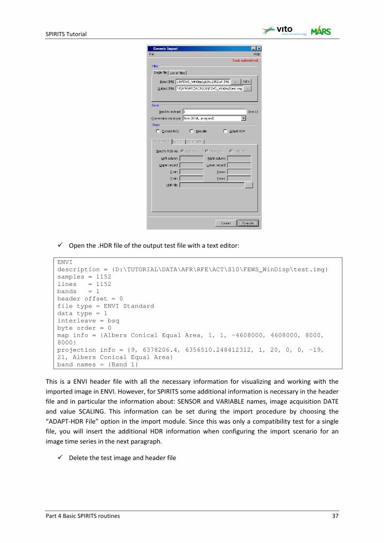
Open Open <Import / Export> <Import> <Generic Import> <Tool> and go to the <Single file> import tab. This is the default option; alternatively lists of files can be imported.

Select one of the WinDisp files in ‘D:\TUTORIAL\DATA\AFR\RFE\ACT\S10\FEWS_WinDisp\’ as input.

Click on <Info>. A separate window will show how the import library (GDAL12) reads the information contained in the input file. The information will give you an idea whether the file format is recognized by the SPIRITS importer. For example, check the information about file size and file projection. Close the info window.

Provide an output name for testing purposes (e.g. ‘D:\TUTORIAL\DATA\AFR\RFE\ACT\S10\FEWS_WinDisp\test.img’) and execute the module by clicking on <Execute>.

12 http://www.gdal.org/gdalinfo.html

http://www.gdal.org/gdalinfo.html

SPIRITS Tutorial


Open the .HDR file of the output test file with a text editor:

ENVI description = {D:\TUTORIAL\DATA\AFR\RFE\ACT\S10\FEWS_WinDisp\test.img} samples = 1152 lines = 1152 bands = 1 header offset = 0 file type = ENVI Standard data type = 1 interleave = bsq byte order = 0 map info = {Albers Conical Equal Area, 1, 1, -4608000, 4608000, 8000, 8000} projection info = {9, 6378206.4, 6356510.248412312, 1, 20, 0, 0, -19, 21, Albers Conical Equal Area} band names = {Band 1}

This is a ENVI header file with all the necessary information for visualizing and working with the imported image in ENVI. However, for SPIRITS some additional information is necessary in the header file and in particular the information about: SENSOR and VARIABLE names, image acquisition DATE and value SCALING. This information can be set during the import procedure by choosing the “ADAPT-HDR File” option in the import module. Since this was only a compatibility test for a single file, you will insert the additional HDR information when configuring the import scenario for an image time series in the next paragraph.

Delete the test image and header file

SPIRITS Tutorial


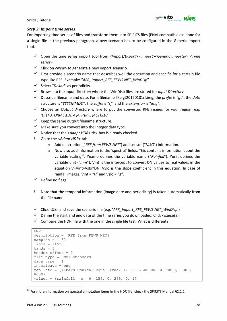
Step 3: Import time series For importing time series of files and transform them into SPIRITS files (ENVI compatible) as done for a single file in the previous paragraph, a new scenario has to be configured in the Generic Import tool.

Open the time series import tool from <Import/Export> <Import><Generic importer> <Time series>.

Click on <New> to generate a new import scenario. First provide a scenario name that describes well the operation and specific for a certain file

type like RFE. Example: “AFR_Import_RFE_FEWS NET_WinDisp” Select “Dekad” as periodicity. Browse to the input directory where the WinDisp files are stored for Input Directory. Describe filename and date. For a filename like gt20120101rf.img, the prefix is “gt”, the date

structure is “YYYYMMDD”, the suffix is “rf” and the extension is “img”. Choose an Output directory where to put the converted RFE images for your region, e.g.

‘D:\TUTORIAL\DATA\AFR\RFE\ACT\S10’. Keep the same output filename structure. Make sure you convert into the Integer data type. Notice that the <Adapt HDR> tick-box is already checked. ! Go to the <Adapt HDR> tab.

o Add description (“RFE from FEWS NET”) and sensor (“MSG”) information. o Now also add information to the ‘spectral’ fields. This contains information about the

variable scaling13. Yname defines the variable name (“Rainfall”). Yunit defines the variable unit (“mm”). Vint is the intercept to convert DN values to real values in the equation V=Vint+Vslo*DN. VSlo is the slope coefficient in this equation. In case of rainfall images, Vint = “0” and Vslo = “1”.

Define no flags.

! Note that the temporal information (image date and periodicity) is taken automatically from the file name.

Click <Ok> and save the scenario file (e.g. ‘AFR_Import_RFE_FEWS NET_WinDisp’) Define the start and end date of the time series you downloaded. Click <Execute>. Compare the HDR file with the one in the single file test. What is different?

ENVI description = {RFE from FEWS NET} samples = 1152 lines = 1152 bands = 1 header offset = 0 file type = ENVI Standard data type = 1 interleave = bsq map info = {Albers Conical Equal Area, 1, 1, -4608000, 4608000, 8000, 8000} values = {rainfall, mm, 0, 255, 0, 255, 0, 1}

13 For more information on spectral annotation items in the HDR file, check the SPIRITS Manual §2.2.2.

SPIRITS Tutorial


date = 20120521 days = 10 sensor type = MSG program = {HDRadapt.exe (V912)}

Importing NetCDF rainfall estimates from TAMSAT You will use the same procedure as in the previous exercise to show you how to import a time series of images in NetCDF format into SPIRITS. As an example you will import a short time series of RFE (rainfall estimate) images over Africa, downloaded from TAMSAT14.

First, download some decadal rainfall estimate images over Africa (in NetCDF format) from the TAMSAT data portal, and store them in ‘D:\TUTORIAL\DATA\AFR\RFE\ACT\S10\TAMSAT_NetCDF\’.

After downloading the data from TAMSAT, these are the steps to be performed:

1. Change of the filenames according to the structure <prefix><date><suffix> 2. Test the import with a single file 3. Import the time series 4. Extraction of the ROI (see Exercise 4-2 p.50)

Step 1: Change the filenames Go to the folder where the downloaded rainfall estimates are stored: e.g.

‘D:\TUTORIAL\DATA\AFR\RFE\ACT\S10\TAMSAT_NetCDF\’.

The structure of the NetCDF filenames is: rfeYYYY_MM-dkD.nc (e.g. rfe2012_09-dk1.nc). This naming structure is not compatible with SPIRITS, because the date format is not one of the predefined SPIRITS date formats. Therefore, you will use the rename tool.

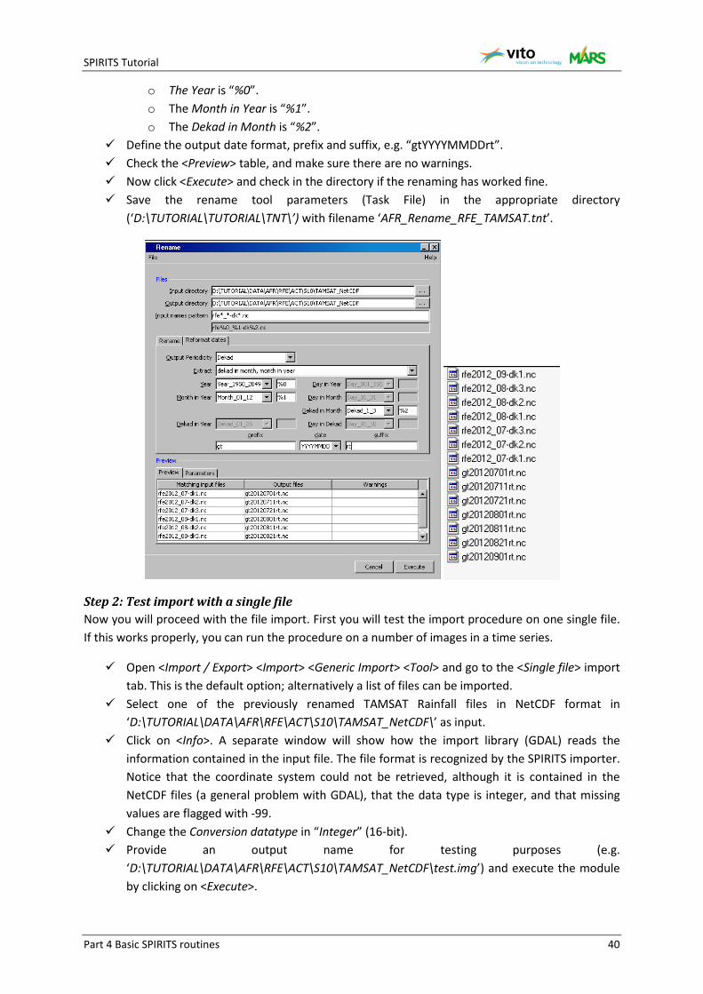
Open the <Rename> tool in the <File> <Files> menu. Define the input and output directory, both as

‘D:\TUTORIAL\DATA\AFR\RFE\ACT\S10\TAMSAT_NetCDF’. Define the input names pattern as “rfe*_*-dk*.nc”. Notice that the rename tool gives the

variable characters a specific code: “rfe%0_%1-dk%2.nc”. You will use this code in the renaming operation.

! Note: The “*” is a placeholder for multiple characters. The “?”, as was used in the previous exercise, is a placeholder for a single character.

Now go to the <Reformat dates> tab. The Output Periodicity is “Dekad” because you are treating 10-daily images.

Choose to extract the date from “Dekad in month, month in year”. o Select <Year_1950_2049> from the drop-down box as the format to be used in Year.

Notice that you now have a 4-digit Year notation in our Input Filenames.

14 Note that the TAMSAT African Rainfall Climatology And Time-series dataset (also referred to as TARCAT Version 2.0) was released in January 2012. The TARCAT (TAMSAT African Rainfall Climatology And Time-series) v2.0 Online Database is available from: http://www.met.reading.ac.uk/~tamsat/data/.

http://www.met.reading.ac.uk/~tamsat/data/

SPIRITS Tutorial


o The Year is “%0”. o The Month in Year is “%1”. o The Dekad in Month is “%2”.

Define the output date format, prefix and suffix, e.g. “gtYYYYMMDDrt”. Check the <Preview> table, and make sure there are no warnings. Now click <Execute> and check in the directory if the renaming has worked fine. Save the rename tool parameters (Task File) in the appropriate directory

(‘D:\TUTORIAL\TUTORIAL\TNT\’) with filename ‘AFR_Rename_RFE_TAMSAT.tnt’.

Step 2: Test import with a single file Now you will proceed with the file import. First you will test the import procedure on one single file. If this works properly, you can run the procedure on a number of images in a time series.

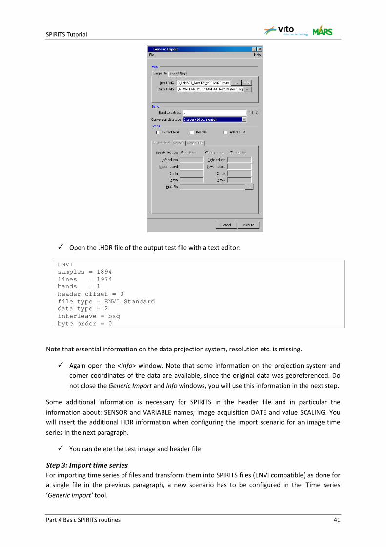
Open <Import / Export> <Import> <Generic Import> <Tool> and go to the <Single file> import tab. This is the default option; alternatively a list of files can be imported.

Select one of the previously renamed TAMSAT Rainfall files in NetCDF format in ‘D:\TUTORIAL\DATA\AFR\RFE\ACT\S10\TAMSAT_NetCDF\’ as input.

Click on <Info>. A separate window will show how the import library (GDAL) reads the information contained in the input file. The file format is recognized by the SPIRITS importer. Notice that the coordinate system could not be retrieved, although it is contained in the NetCDF files (a general problem with GDAL), that the data type is integer, and that missing values are flagged with -99.

Change the Conversion datatype in “Integer” (16-bit). Provide an output name for testing purposes (e.g.

‘D:\TUTORIAL\DATA\AFR\RFE\ACT\S10\TAMSAT_NetCDF\test.img’) and execute the module by clicking on <Execute>.

SPIRITS Tutorial


Open the .HDR file of the output test file with a text editor:

ENVI samples = 1894 lines = 1974 bands = 1 header offset = 0 file type = ENVI Standard data type = 2 interleave = bsq byte order = 0

Note that essential information on the data projection system, resolution etc. is missing.

Again open the <Info> window. Note that some information on the projection system and corner coordinates of the data are available, since the original data was georeferenced. Do not close the Generic Import and Info windows, you will use this information in the next step.

Some additional information is necessary for SPIRITS in the header file and in particular the information about: SENSOR and VARIABLE names, image acquisition DATE and value SCALING. You will insert the additional HDR information when configuring the import scenario for an image time series in the next paragraph.

You can delete the test image and header file

Step 3: Import time series For importing time series of files and transform them into SPIRITS files (ENVI compatible) as done for a single file in the previous paragraph, a new scenario has to be configured in the 'Time series ‘Generic Import’ tool.

SPIRITS Tutorial


Open the time series import tool from <Import/Export> <Import><Generic importer> <Time series>.

Click on <New> to generate a new import scenario. First provide a scenario name that describes well the operation and specific for a certain file

type like RFE, such as e.g.: “AFR_Import_RFE_TAMSAT_NetCDF” Select <Dekad> as Periodicity. Browse to the input directory where the renamed NetCDF files are stored. Describe filename and date. For a filename like “gt20120101rt.nc”,

o Prefix is “gt”. o Date structure is “YYYYMMDD”. o Suffix is “rt”. o Extension is “nc”.

Choose an output directory where to put the converted RFE images for your region, e.g. ‘D:\TUTORIAL\DATA\AFR\RFE\ACT\S10\TAMSAT_NetCDF\Imported’.

Keep the same output filename structure.

Go to the <Adapt HDR> tab. o Add a Description (“RFE from TAMSAT”) and Sensor (“MSG”). o In the Spatial section15, add the following data:

Map Info: “Geographic Lat/Lon” Magic column: “1” Magic record: “1” Magic X: “-19.0125” (this is the ‘lonmin’ from the NetCDF metadata) Magic Y: “38.025” (this is the ‘latmax’ from the NetCDF metadata) X-resolution: “0.0375” Y-resolution: “0.0375”

o Now also add information to the ‘spectral’ fields. This contains information about the variable scaling16. Yname defines the variable name (“Rainfall”). Yunit defines the variable unit (“mm”). Vint is the intercept to convert DN values to real values in the equation V=Vint+Vslo*DN. VSlo is the slope coefficient in this equation. In case of rainfall images, Vint = “0” and Vslo = “1”. The no data flag (Flags) is “-99”.

! Note that the temporal information (image date and periodicity) is taken automatically from the file name.

15 For more information on the spatial-geographic annotation in the HDR files, check the SPIRITS manual §2.1.4 16 For more information on spectral annotation items in the HDR file, check the SPIRITS Manual §2.2.2.

SPIRITS Tutorial


Click <Ok> and save the scenario file (e.g. ‘AFR_Import_RFE_TAMSAT_NetCDF’) Define the start and end date of the time series you downloaded. Click <Execute>. Compare the HDR file with the one in the single file test. What is different?

ENVI description = {RFE from TAMSAT} samples = 1894 lines = 1974 bands = 1 header offset = 0 file type = ENVI Standard data type = 2 interleave = bsq byte order = 0 map info = {Geographic Lat/Lon, 1, 1, -19.0125, 38.025, 0.0375, 0.0375} values = {rainfall, mm, -32768, 32767, -32768, 32767, 0, 1} flags = {-99} date = 20120821 days = 10 sensor type = MSG program = {HDRadapt.exe (V912)}

SPIRITS Tutorial


Importing HDF files from DevCoCast In this exercise, SPOT-VGT NDVI products are extracted using VGTExtract, and prepared for use in SPIRITS. The VGTExtract tool is a simple and free utility used for the automated integration of basic and derived SPOT-VEGETATION products in a variety of GIS and Remote Sensing end-user software for further analysis, processing or visualization. The VGT NDVI images can be downloaded from the DevCoCast website (http://www.DevCoCast.eu)17.

After getting the data (which consists of several HDF layers joined in one ZIP file), these are the steps to be performed:

1. Extraction of the NDVI product and the so-called ‘Status Map’ using VGTExtract software. This software is freely available for download on www.agricab.info.

2. Applying the Status Map on the NDVI image in SPIRITS using the ‘Flag VGT NDVI’ tool.

Step 1: Convert the HDF into ENVI format using VGTExtract The first step is the extraction of the NDVI product and the ‘Status Map’ using VGTExtract18.

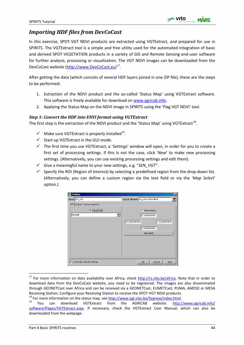
Make sure VGTExtract is properly installed19. Start up VGTExtract in the GUI mode. The first time you use VGTExtract, a ‘Settings’ window will open, in order for you to create a

first set of processing settings. If this is not the case, click ‘New’ to make new processing settings. (Alternatively, you can use existing processing settings and edit them).

Give a meaningful name to your new settings, e.g. “SEN_VGT”. Specify the ROI (Region of Interest) by selecting a predefined region from the drop-down list.

(Alternatively, you can define a custom region via the text field or via the ‘Map Select’ option.)

17 For more information on data availability over Africa, check http://rs.vito.be/africa. Note that in order to download data from the DevCoCast website, you need to be registered. The images are also disseminated through GEONETCast over Africa and can be received via a GEONETCast, EUMETCast, PUMA, AMESD or MESA Receiving Station. Configure your Receiving Station to receive the SPOT-VGT NDVI products. 18 For more information on the status map, see http://www.vgt.vito.be/faqnew/index.html. 19 You can download VGTExtract from the AGRICAB website: http://www.agricab.info/ software/Pages/VGTExtract.aspx. If necessary, check the VGTExtract User Manual, which can also be downloaded from the webpage.

http://www.devcocast.eu/

http://www.agricab.info/

http://rs.vito.be/africa

http://www.vgt.vito.be/faqnew/index.html

http://www.agricab.info/software/Pages/VGTExtract.aspx

http://www.agricab.info/software/Pages/VGTExtract.aspx

SPIRITS Tutorial


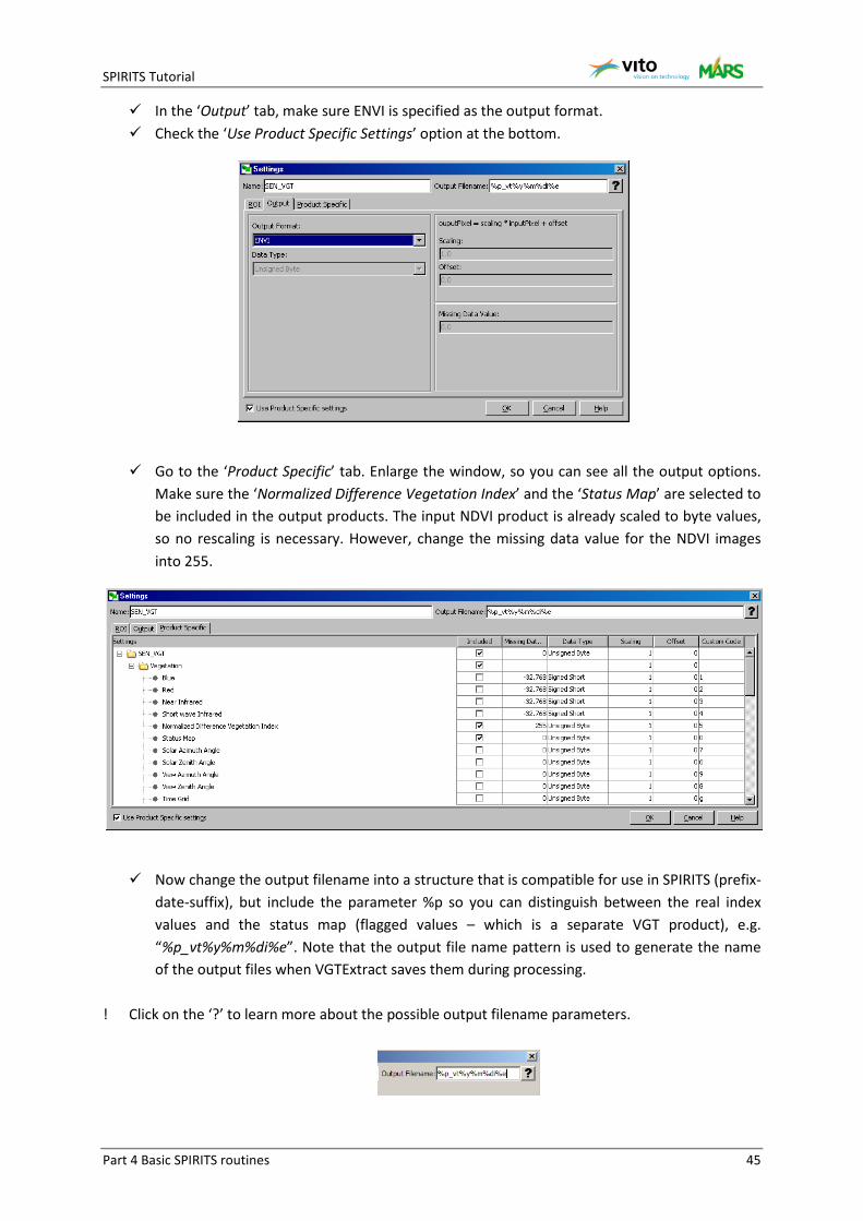
In the ‘Output’ tab, make sure ENVI is specified as the output format. Check the ‘Use Product Specific Settings’ option at the bottom.

Go to the ‘Product Specific’ tab. Enlarge the window, so you can see all the output options.

Make sure the ‘Normalized Difference Vegetation Index’ and the ‘Status Map’ are selected to be included in the output products. The input NDVI product is already scaled to byte values, so no rescaling is necessary. However, change the missing data value for the NDVI images into 255.

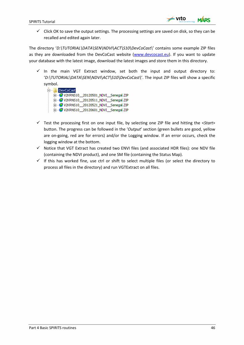
Now change the output filename into a structure that is compatible for use in SPIRITS (prefix-

date-suffix), but include the parameter %p so you can distinguish between the real index values and the status map (flagged values – which is a separate VGT product), e.g. “%p_vt%y%m%di%e”. Note that the output file name pattern is used to generate the name of the output files when VGTExtract saves them during processing.

! Click on the ‘?’ to learn more about the possible output filename parameters.

SPIRITS Tutorial


Click OK to save the output settings. The processing settings are saved on disk, so they can be recalled and edited again later.

The directory ‘D:\TUTORIAL\DATA\SEN\NDVI\ACT\S10\DevCoCast\’ contains some example ZIP files as they are downloaded from the DevCoCast website (www.devcocast.eu). If you want to update your database with the latest image, download the latest images and store them in this directory.

In the main VGT Extract window, set both the input and output directory to: ‘D:\TUTORIAL\DATA\SEN\NDVI\ACT\S10\DevCoCast\’. The input ZIP files will show a specific symbol.

Test the processing first on one input file, by selecting one ZIP file and hitting the <Start> button. The progress can be followed in the ‘Output’ section (green bullets are good, yellow are on-going, red are for errors) and/or the Logging window. If an error occurs, check the logging window at the bottom.

Notice that VGT Extract has created two ENVI files (and associated HDR files): one NDV file (containing the NDVI product), and one SM file (containing the Status Map).

If this has worked fine, use ctrl or shift to select multiple files (or select the directory to process all files in the directory) and run VGTExtract on all files.

http://www.devcocast.eu/

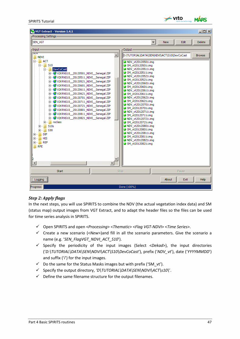
SPIRITS Tutorial


Step 2: Apply flags In the next steps, you will use SPIRITS to combine the NDV (the actual vegetation index data) and SM (status map) output images from VGT Extract, and to adapt the header files so the files can be used for time series analysis in SPIRITS.

Open SPIRITS and open <Processing> <Thematic> <Flag VGT-NDVI> <Time Series>. Create a new scenario (<New>)and fill in all the scenario parameters. Give the scenario a

name (e.g. ‘SEN_FlagVGT_NDVI_ACT_S10’). Specify the periodicity of the input images (Select <Dekad>), the input directories

(‘D:\TUTORIAL\DATA\SEN\NDVI\ACT\S10\DevCoCast’), prefix (‘NDV_vt’), date (‘YYYYMMDD’) and suffix (‘i’) for the input images.

Do the same for the Status Masks images but with prefix (‘SM_vt’). Specify the output directory, ‘D\TUTORIAL\DATA\SEN\NDVI\ACT\s10\’. Define the same filename structure for the output filenames.

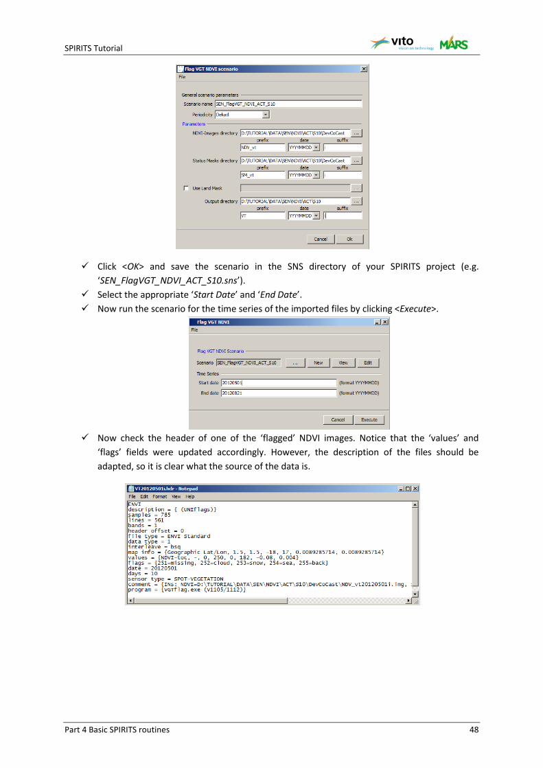
SPIRITS Tutorial


Click <OK> and save the scenario in the SNS directory of your SPIRITS project (e.g. ‘SEN_FlagVGT_NDVI_ACT_S10.sns’).

Select the appropriate ‘Start Date’ and ‘End Date’. Now run the scenario for the time series of the imported files by clicking <Execute>.

Now check the header of one of the ‘flagged’ NDVI images. Notice that the ‘values’ and

‘flags’ fields were updated accordingly. However, the description of the files should be adapted, so it is clear what the source of the data is.

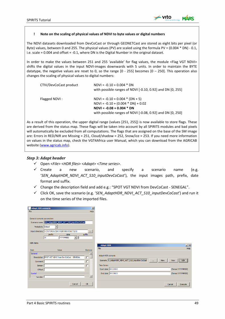
SPIRITS Tutorial


! Note on the scaling of physical values of NDVI to byte values or digital numbers

The NDVI datasets downloaded from DevCoCast or through GEONETCast are stored as eight bits per pixel (or Byte) values, between 0 and 255. The physical values (PV) are scaled using the formula PV = (0.004 * DN) - 0.1, i.e. scale = 0.004 and offset = -0.1, where DN is the Digital Number in the original dataset. In order to make the values between 251 and 255 ‘available’ for flag values, the module <Flag VGT NDVI> shifts the digital values in the input NDVI-images downwards with 5 units. In order to maintain the BYTE datatype, the negative values are reset to 0, so the range [0 - 255] becomes [0 – 250]. This operation also changes the scaling of physical values to digital numbers:

CTIV/DevCoCast product NDVI = -0.10 + 0.004 * DN with possible ranges of NDVI [-0.10, 0.92] and DN [0, 255] Flagged NDVI : NDVI = -0.10 + 0.004 * (DN + 5)

NDVI = -0.10 + (0.004 * DN) + 0.02 NDVI = -0.08 + 0.004 * DN

with possible ranges of NDVI [-0.08, 0.92] and DN [0, 250] As a result of this operation, the upper digital range (values [251, 255]) is now available to store flags. These are derived from the status map. These flags will be taken into account by all SPIRITS modules and bad pixels will automatically be excluded from all computations. The flags that are assigned on the base of the SM image are: Errors in RED/NIR are Missing = 251, Cloud/shadow = 252, Snow/ice = 253. If you need more information on values in the status map, check the VGT4Africa user Manual, which you can download from the AGRICAB website (www.agricab.info).

Step 3: Adapt header Open <File> <HDR files> <Adapt> <Time series>. Create a new scenario, and specify a scenario name (e.g.

‘SEN_AdaptHDR_NDVI_ACT_S10_inputDevCoCast’), the input images path, prefix, date format and suffix.

Change the description field and add e.g.: “SPOT VGT NDVI from DevCoCast - SENEGAL”. Click OK, save the scenario (e.g. ‘SEN_AdaptHDR_NDVI_ACT_S10_inputDevCoCast’) and run it

on the time series of the imported files.

http://www.agricab.info/

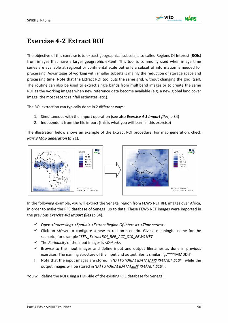
SPIRITS Tutorial


Exercise 4-2 Extract ROI

The objective of this exercise is to extract geographical subsets, also called Regions Of Interest (ROIs) from images that have a larger geographic extent. This tool is commonly used when image time series are available at regional or continental scale but only a subset of information is needed for processing. Advantages of working with smaller subsets is mainly the reduction of storage space and processing time. Note that the Extract ROI tool cuts the same grid, without changing the grid itself. The routine can also be used to extract single bands from multiband images or to create the same ROI as the working images when new reference data become available (e.g. a new global land cover image, the most recent rainfall estimates, etc.).

The ROI extraction can typically done in 2 different ways:

1. Simultaneous with the import operation (see also Exercise 4-1 Import files, p.34) 2. Independent from the file import (this is what you will learn in this exercise)

The illustration below shows an example of the Extract ROI procedure. For map generation, check Part 3 Map generation (p.21).

In the following example, you will extract the Senegal region from FEWS NET RFE images over Africa, in order to make the RFE database of Senegal up to date. These FEWS NET images were imported in the previous Exercise 4-1 Import files (p.34).

Open <Processing> <Spatial> <Extract Region Of Interest> <Time series>. Click on <New> to configure a new extraction scenario. Give a meaningful name for the

scenario, for example “SEN_ExtractROI_RFE_ACT_S10_FEWS NET”. The Periodicity of the input images is <Dekad>. Browse to the input images and define input and output filenames as done in previous

exercises. The naming structure of the input and output files is similar: ‘gtYYYYMMDDrf’. ! Note that the input images are stored in ‘D:\TUTORIAL\DATA\AFR\RFE\ACT\S10\’, while the

output images will be stored in ‘D:\TUTORIAL\DATA\SEN\RFE\ACT\S10\’.

You will define the ROI using a HDR-file of the existing RFE database for Senegal.

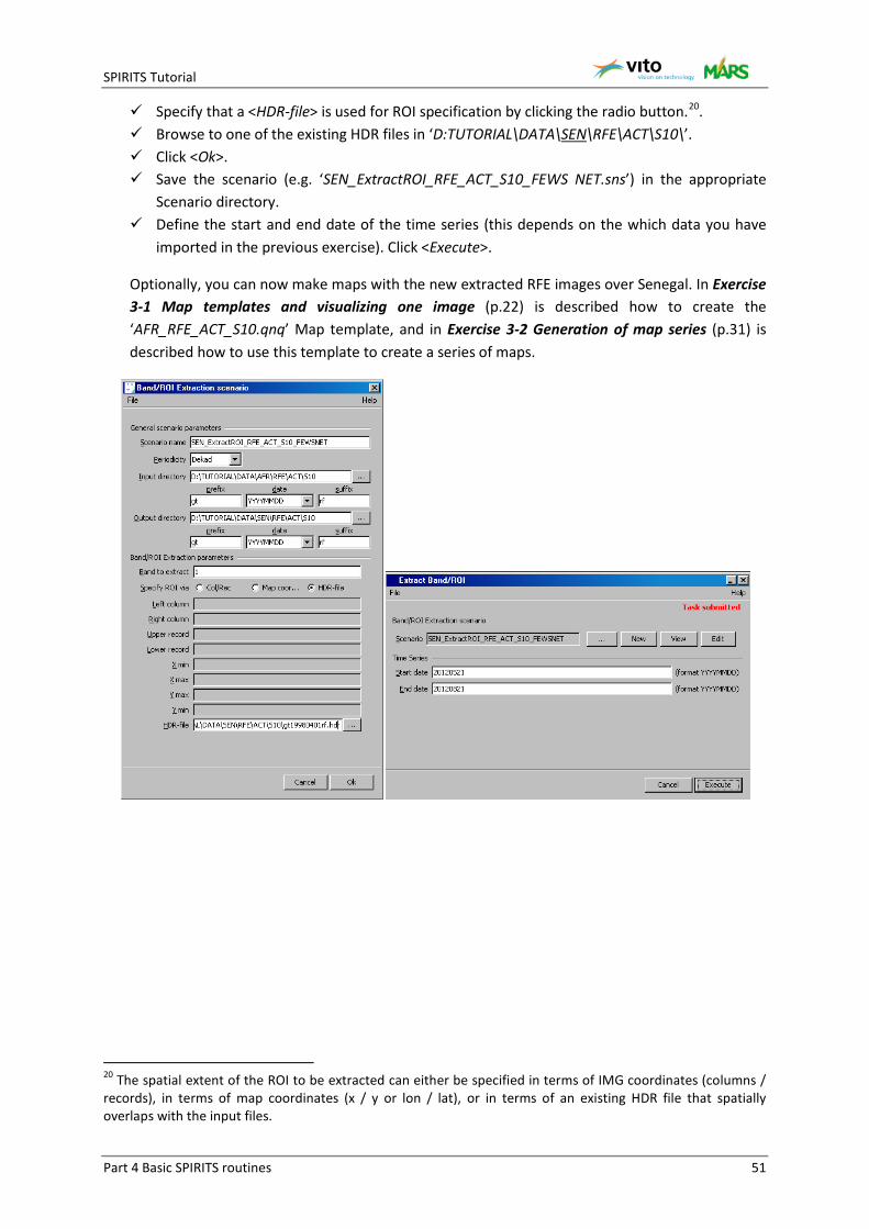
SPIRITS Tutorial


Specify that a <HDR-file> is used for ROI specification by clicking the radio button.20. Browse to one of the existing HDR files in ‘D:TUTORIAL\DATA\SEN\RFE\ACT\S10\’. Click <Ok>. Save the scenario (e.g. ‘SEN_ExtractROI_RFE_ACT_S10_FEWS NET.sns’) in the appropriate

Scenario directory. Define the start and end date of the time series (this depends on the which data you have

imported in the previous exercise). Click <Execute>.

Optionally, you can now make maps with the new extracted RFE images over Senegal. In Exercise 3-1 Map templates and visualizing one image (p.22) is described how to create the ‘AFR_RFE_ACT_S10.qnq’ Map template, and in Exercise 3-2 Generation of map series (p.31) is described how to use this template to create a series of maps.

20 The spatial extent of the ROI to be extracted can either be specified in terms of IMG coordinates (columns / records), in terms of map coordinates (x / y or lon / lat), or in terms of an existing HDR file that spatially overlaps with the input files.

SPIRITS Tutorial


Exercise 4-3 Thinning

The IMG thinning tool can perform two operations at the same time: the extraction of a region of interest (optional, comparable to the operation in Exercise 4-2 Extract ROI), and the degradation of the spatial resolution through pixel thinning. The window size of the filter applied on the input IMG defines the factor of the spatial resolution degradation. For example, an image with 100 columns and 100 records can be contracted to an image of 25 columns by 25 records, if a filter with 4 pixels size is applied.

Thinning of a classification image The following two examples show the application of the Thinning operation for a classification image (images with a limited number of discrete classes).

The figure below illustrates the thinning operation on a land cover map over Senegal21. A filter of 10 by 10 pixels is applied, and the ‘Mode’ operation is performed. The result is an image with 10 times less columns and records. The pixel value (land cover class) is equal to the class that is most abundant in each 10 x 10 pixel (filter) window.

Open <Processing> <Spatial> <Thinning> <Tool>. As input image, use ‘D:\TUTORIAL\TUTORIAL\DATA\SEN\NDVI\REF\GLC_5classes.img’ Store the output image ‘GLC_5classes_thin10.img’ in the same folder:

‘D:\TUTORIAL\TUTORIAL\DATA\SEN\NDVI\REF\’. Keep the same ROI, go to the Filter part of the Window. Use a “10” pixels wide Window size. Use the <Mode> filter: the most abundant land cover class in the 10 x 10 pixel window will be

kept in the output image, whenever there are for example 50% ‘good’ values in the input pixel window. This is the most common approach for thinning of classified images.

The Minimum % of ‘good’ values in window is “50”.

21 In this exercise we use a reclassified GLC2000 map over Africa, based on: Mayaux, P., Bartholomé, E., Massart, M., Van Cutsem, C., Cabral, A., Nonguierma, A., Diallo, O., Pretorius, C., Thompson, M., Cherlet, M., Pekel, J.-F., Defourny, P., Vasconcelos, M., Di Gregorio, A., Fritz, S., De Grandi, G., Elvidge, C., Vogt, P., Belward, A., 2003. A land cover map of Africa, European Commission - JRC.

SPIRITS Tutorial


The Flag value for ‘bad’ output pixels is “0”. The number of bins22 is equal to the number of classes in the input image: “5”. Save the Thinning task as ‘SEN_Thinning_GLC5.tnt’ in our Task directory (‘TNT’) and click

<Execute>. Visualize the input image and the resulting image in the Map generator (see Part 3 Map

generation). You can also test other filter operations, which will all result in a slightly different output

product: o In the ‘Systematic’ operation (Select the <Systematic> tab), in each filter window a

certain pixel is kept in the output image. E.g. if you specify to select column 6 and record 4, the output pixel value is determined by only one pixel value in the 10 x 10 filter window, as illustrated below.

o In the ‘Random’ operation, a random value in the input filter window is kept in the

output image.

Example of the ‘Systematic’ image thinning

operation with systematic selection of column 6 and record 4.

Example of the ‘Random’ image thinning

operation.

Thinning of vegetation indicator images The figure below illustrates the thinning operation on an NDVI image over Senegal. A filter of 10 by 10 pixels is applied, and the ‘Mean’ operation is performed. The result is an image with 10 times less columns and records, and the pixel value is equal to the mean value of the 100 pixels in each 10 x 10 pixel (filter) window.

22 The Mode operation is computed on the input data, which are first grouped in a number of bins with equal width. In case of a classified image, the number of bins is therefore equal to the number of classes.

SPIRITS Tutorial


Open <Processing> <Spatial> <Thinning> <Time series>. Create a <New> scenario and name it ‘SEN_Thinning_NDVI_ACT_S10’. The Periodicity of the input images is “Dekad”. The input images are stored in the ‘D:\TUTORIAL\DATA\SEN\NDVI\ACT\S10’ directory. Check the filenames to find out the prefix, date and suffix information. Enter prefix “vt”, date

format “YYYYMMDD”, and suffix “i”. The output can be stored in the ‘D:\TUTORIAL\DATA\SEN\NDVI\ACT\S10\Thinned’ directory,

with same prefix and date format, but change the suffix into “it”. Do not forget to create the directory first.

You will use the same ROI as the input images. Therefore, specify the ROI using one of the HDR files of the input series.

Use a “10” pixels wide Window size. Use the <Mean> filter. The pixel value in the output is equal to the mean value of the pixels

in each 10 x 10 pixel (filter) window, whenever there are for example “50” percent ‘good’ values in the input pixel window.

The Flag value for ‘bad’ output pixels is “255”. Click <Ok> and save the Thinning scenario as ‘SEN_Thinning_NDVI_ACT_S10’ in the

‘D:\TUTORIAL\SNS\’ directory. Run the scenario on a short time series (e.g. 20120501 till now), and follow the process in the

Tasks queue. Visualize one of the input image and one of the resulting images in the Map generator (see

Part 3 Map generation).

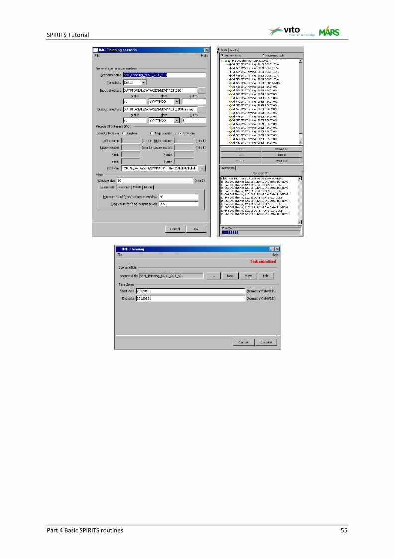
SPIRITS Tutorial


SPIRITS Tutorial


Exercise 4-4 Area Fraction Images

The Area Fraction Images tool is used to create area fraction images (AFIs) based on a higher resolution land cover map. An AFI contains pixel values (0...100) that represent the percentage of a specific land cover class. The tool can perform two operations at the same time: the extraction of a region of interest (optional, comparable to the operation in Exercise 4-2 Extract ROI), and the degradation of the spatial resolution through creation of a series of AFIs: for each land cover class an AFI is created, whereby the pixel value represents the percentage of the specific land cover class contained in the larger pixel.

In this exercise, you will use resampled GlobCover23 maps over Senegal. The resulting AFIs can later be used for statistics extraction, see Part 7 Extraction of statistics (p.95).GlobCover is an ESA initiative which began in 2005 in partnership with JRC, EEA, FAO, UNEP, GOFC-GOLD and IGBP. The aim of the project was to develop a service capable of delivering global composites and land cover maps using as input observations from the 300m MERIS sensor on board the ENVISAT satellite mission.

The first GlobCover map used in this exercise has a spatial resolution that is exactly 3 times higher (i.e. pixels are 3 times smaller) than the SPOT-Vegetation NDVI images.

Open <Processing> <Spatial> <Area Fraction IMGs>. As input IMG, specify “GlobCover_resampled.img” in the ‘D:\TUTORIAL\DATA\SEN\NDVI\REF’

directory. As output directory, choose ‘D:\TUTORIAL\DATA\SEN\NDVI\REF\GlobCover_AFI’ (if

necessary, make a new folder). The prefix of the filenames is “Globcover_AFI”. The output AFI datatype can be byte: byte values between 0 and 200 will refer to ‘physical’

values of 0 to 100%, with scaling factor (slope) 0.5. Use the ‘resampling’ procedure, and use one of the actual NDVI images over Senegal as a

reference for output framing. Save the task (<File> <Save As>) as ‘SEN_GlobCover_AFI_NDVI.tnt’ and click <Execute>.

23 Arino, O., Gross, D., Ranera, F., Bourg, L., Leroy, M., Bicheron, P., Latham, J., Di Gregorio, A., Brockman, C., Witt, R., Defourny, P., Van Cutsem, C., Herold, M., Sambale, J., Achard, F., Durieux, L., Plummer, S., Weber, J.-L., 2007. GlobCover: ESA service for global land cover from MERIS, International Geoscience and Remote Sensing Symposium, 23-28 July 2007, Barcelona, Spain.

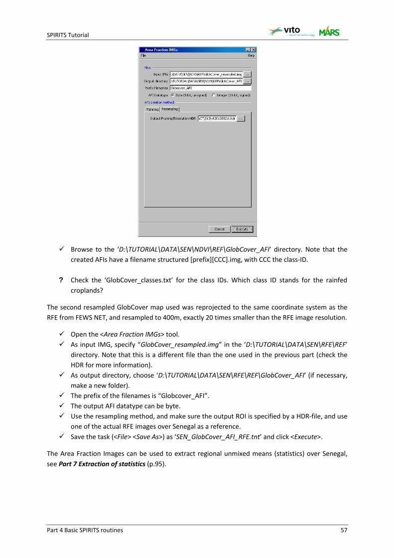
SPIRITS Tutorial


Browse to the ‘D:\TUTORIAL\DATA\SEN\NDVI\REF\GlobCover_AFI’ directory. Note that the created AFIs have a filename structured [prefix][CCC].img, with CCC the class-ID.

? Check the ‘GlobCover_classes.txt’ for the class IDs. Which class ID stands for the rainfed croplands?

The second resampled GlobCover map used was reprojected to the same coordinate system as the RFE from FEWS NET, and resampled to 400m, exactly 20 times smaller than the RFE image resolution.

Open the <Area Fraction IMGs> tool. As input IMG, specify “GlobCover_resampled.img” in the ‘D:\TUTORIAL\DATA\SEN\RFE\REF’

directory. Note that this is a different file than the one used in the previous part (check the HDR for more information).

As output directory, choose ‘D:\TUTORIAL\DATA\SEN\RFE\REF\GlobCover_AFI’ (if necessary, make a new folder).

The prefix of the filenames is “Globcover_AFI”. The output AFI datatype can be byte. Use the resampling method, and make sure the output ROI is specified by a HDR-file, and use

one of the actual RFE images over Senegal as a reference. Save the task (<File> <Save As>) as ‘SEN_GlobCover_AFI_RFE.tnt’ and click <Execute>.

The Area Fraction Images can be used to extract regional unmixed means (statistics) over Senegal, see Part 7 Extraction of statistics (p.95).

SPIRITS Tutorial


Exercise 4-5 Image reclassification and scaling

The image reclassification tool of SPIRITS is used to reclassify or rescale the actual pixel values in the IMG.

Several spectral conversions can be done at the same time: convert the data type, reset a range of values to one output value, change the linear scaling of values, histogram equalization etc. For every image reclassification and scaling operation, the parameters are defined in an SPS (scaling specification) file. For more information on the SPS files, check the SPIRITS Manual. This tool can also be used to change scaled values (digital numbers) into physical values, which might be useful when exporting to other software.

The following exercises show you how to

- Reclassify a single NDVI image into discrete classes. - Change the data type of a TAMSAT rainfall estimate map from integer to byte.

Reclassification of an NDVI image You will learn how to reclassify an NDVI image in three classes: low NDVI (< 0.4), middle NDVI (0.4 .. 0.7) and high NDVI (> 0.7).

Open <Processing> <Thematic> <Scaling> <Tool>. Select one NDVI image of Senegal as input file (in ‘D:\TUTORIAL\DATA\SEN\NDVI\ACT\S10\’),

and specify an output image e.g. in ‘D:\TUTORIAL\DATA\SEN\NDVI\ACT\S10\reclass\’. Do not forget to create the directory first.

Make a <New> SPS specification file. Both the input and output data type are “Byte”. Add four slices (<Add Slice>):

o The first three slices will be used to “Copy IN-values to constant”. o Note that the thresholds are defined as the byte values in the input images. Since the

NDVI is scaled as NDVI = -0.08 + 0.004 * V, the thresholds 0.4 and 0.7 refer to V=120 and V=195, respectively.

o The first threshold “0” is already automatically provided. Define the two thresholds (“120” and “195”) and the three output values (“1”, “2” and “3”).

o The fourth slice is used to copy the input flag values (remember, our flags are all above 250) to the output image. Use “Straight copy of IN-value” with a threshold of “250”.

o Check the Slice Intervals and see to which intervals the values 120 and 195 belong. (Interval#1 = [0-120[, Interval#2 = [120-195[ and Interval#3 = [195, Max])

Click <Ok> and save the SPS file as “scaling_NDVI_3classes.sps” in the relevant directory. Click <Execute>

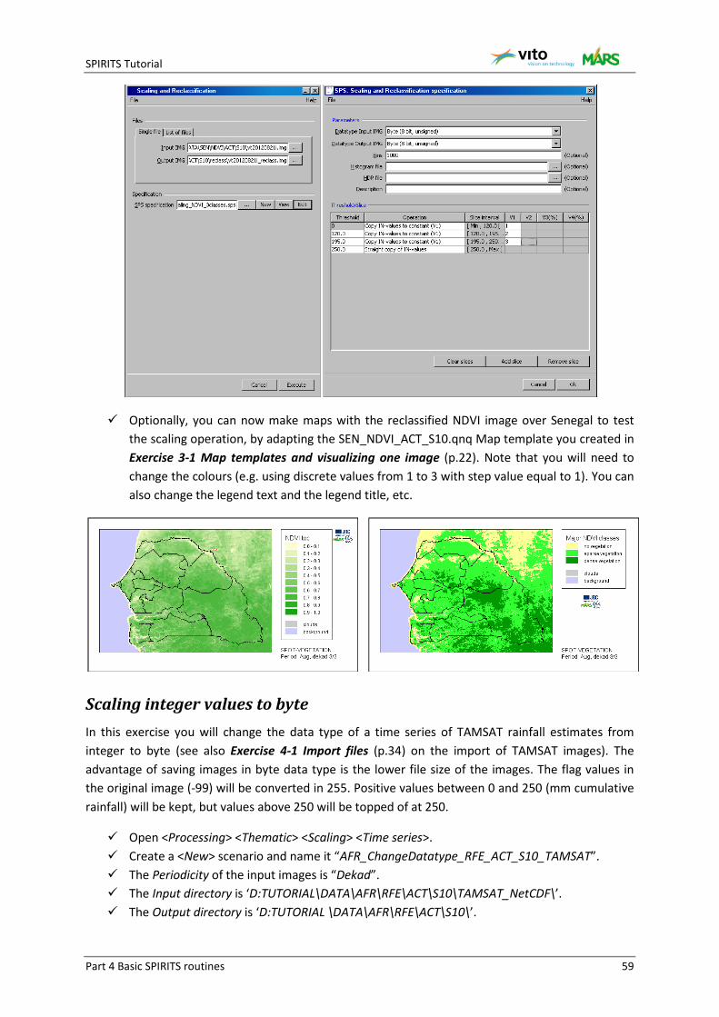
SPIRITS Tutorial


Optionally, you can now make maps with the reclassified NDVI image over Senegal to test the scaling operation, by adapting the SEN_NDVI_ACT_S10.qnq Map template you created in Exercise 3-1 Map templates and visualizing one image (p.22). Note that you will need to change the colours (e.g. using discrete values from 1 to 3 with step value equal to 1). You can also change the legend text and the legend title, etc.

Scaling integer values to byte In this exercise you will change the data type of a time series of TAMSAT rainfall estimates from integer to byte (see also Exercise 4-1 Import files (p.34) on the import of TAMSAT images). The advantage of saving images in byte data type is the lower file size of the images. The flag values in the original image (-99) will be converted in 255. Positive values between 0 and 250 (mm cumulative rainfall) will be kept, but values above 250 will be topped of at 250.

Open <Processing> <Thematic> <Scaling> <Time series>. Create a <New> scenario and name it “AFR_ChangeDatatype_RFE_ACT_S10_TAMSAT”. The Periodicity of the input images is “Dekad”. The Input directory is ‘D:TUTORIAL\DATA\AFR\RFE\ACT\S10\TAMSAT_NetCDF\’. The Output directory is ‘D:TUTORIAL \DATA\AFR\RFE\ACT\S10\’.

SPIRITS Tutorial


Check the file naming structure of your input files and enter prefix, date format and suffix. (Should be “gtYYYYMMDDrt”).

Keep the same filename structure for the output images. Create a <New> SPS specification file. The data type of the input image is “Integer”, while the output will be “Byte”. Add five slices:

o The 1st slice will copy all values from -32768 till -99 to the new constant “0”. (Choose “Copy IN-values to constant (V1)” and V1=”0”. The Threshold of first slice was pre-filled with the minimum value, the Threshold of the second slice shall be “-99”.)

o The 2nd slice copies the flag value “-99” (=IN-value) in the input to the output constant “255”. (Threshold of third slice= “-98”)

o The 3rd slice copies all values from -98 to 0 to the output constant V1 with value “0”. o The 4th slice performs a “Straight copy of the IN-values” on the values between 0 and

250. o The 5th slice copies all input values above 250 to the output constant “250”. This

means all values above 250 are truncated. (Again, use the “Copy IN-values to constant (V1)” with V1=”250”)

Click <Ok> and save the SPS (Specification for Scaling) file as ‘reformat_RFE_TAMSAT.sps’. Again click <Ok> and save the scenario as ‘AFR_ChangeDatatype_RFE_ACT_S10_TAMSAT’ Run the scenario on the imported TAMSAT images

In Windows Explorer, check the difference between the image size of one of the integer images and one of the Byte images.

SPIRITS Tutorial


Exercise 4-6 Rasterize Shapefiles

You will rasterize the ESRI Shapefile (SHP) containing the regions of Senegal to an ENVI raster image file (IMG), in order to use it in some of the following exercises, such as masking (Exercise 4-7 p.63) and the extraction of statistics (Part 7 p.95). The rasterizing tool is based on the GDAL_rasterize utility. The figure below illustrates the operation: at the left the Shapefile with the regions of Senegal as visualized in ArcGIS (note the attribute used for colour coding); at the right the result after the rasterizing operation in SPIRITS.

You will run the rasterize operation twice, in order to create two regions images compatible (in coordinate system, resolution, and extent) with the NDVI time series and with the RFE time series over Senegal, respectively.

Open the <Import / Export> <Vectors><Rasterize SHP> tool. As input SHP, choose the ‘regions.shp’ file in the ‘D:\TUTORIAL\DATA\SEN\NDVI\REF\‘

directory. Check whether the input file is recognized by the gdal_rasterize utility by clicking on the

<Info> button. Save the output IMG in the same directory, e.g. choose as output IMG filename:

‘D:\TUTORIAL\DATA\SEN\NDVI\REF\regions.img’ The framing of the output image file can be specified based on corner coordinates and

resolution, corner coordinates and number of rows and columns, or by using another HDR file. In this case you will use one of the NDVI header files, so the output IMG from the rasterizing process will have the same framing as the NDVI images. Choose one of the header files in the ‘D:\TUTORIAL\DATA\SEN\NDVI\ACT\S10\’ as reference.

Specify the output parameters. You will use the region ID as attribute in the output raster image. The data type of the output image can thus be “Byte” (if the IDs have numbers < 255).

Select one column of the SHP attribute table output attribute: <SHORT_ID1>, which contains an ID of the different regions (click on to open the attribute selection panel, select the ID column <SHORT_ID1> and click <Ok>).

Note that the No data flag is “0”, since the IDs start from 1. This is important for Exercise 4-7 Masking.

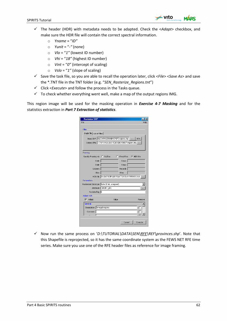
SPIRITS Tutorial


The header (HDR) with metadata needs to be adapted. Check the <Adapt> checkbox, and make sure the HDR file will contain the correct spectral information.

o Yname = “ID” o Yunit = “-“ (none) o Vlo = “1” (lowest ID number) o Vhi = “18” (highest ID number) o Vint = “0” (intercept of scaling) o Vslo = “1” (slope of scaling)

Save the task file, so you are able to recall the operation later, click <File> <Save As> and save the *.TNT file in the TNT folder (e.g. “SEN_Rasterize_Regions.tnt”)

Click <Execute> and follow the process in the Tasks queue. To check whether everything went well, make a map of the output regions IMG.

This region image will be used for the masking operation in Exercise 4-7 Masking and for the statistics extraction in Part 7 Extraction of statistics.

Now run the same process on ‘D:\TUTORIAL\DATA\SEN\RFE\REF\provinces.shp’. Note that this Shapefile is reprojected, so it has the same coordinate system as the FEWS NET RFE time series. Make sure you use one of the RFE header files as reference for image framing.

SPIRITS Tutorial


Exercise 4-7 Masking

In the masking operation, you will use one image (in this case the image with the regions of Senegal, created in Exercise 4-6 Rasterize Shapefiles) to mask out a region or country (in this case Senegal) in a series of 10-daily NDVI images. The figure below illustrates the operation: at the left a map of one of the NDVI images over Senegal (see Part 3 Map generation); at the right the result after the masking operation.

Open <Processing> <Thematic> <Simple masking> <Time series>. Create a <New> scenario, and name it “SEN_Mask_NDVI_ACT_S10”. The Periodicity of the input images is “Dekad”. The input directory is ‘D:\TUTORIAL\DATA\SEN\NDVI\ACT\S10’, prefix is “vt”, date is

“YYYYMMDD” and suffix is “i”. Save the masked output images in the ‘D:\TUTORIAL\DATA\SEN\NDVI\ACT\S10m\’ directory.

Prefix and date format remain the same, but change the suffix in “im” As Mask image, use the “regions.img” you created in Exercise 4-6 Rasterize Shapefiles. Now specify the Lower and Upper mask value. Pixels with a value in the mask image within

this range will be flagged in the out image. Define “0” as both the lower and upper mask value, since this is the “no data flag” value in the regions image.

Specify “255” as Output flag (i.e. background). Click <Ok> and save the scenario as “SEN_Mask_NDVI_ACT_S10.sns”. <Execute> the Mask operation on the entire NDVI time series (19980401 - ...) and follow the

task progress in the Tasks queue. Open the Map template for NDVI images as you created in Exercise 3-1 Map templates and

visualizing one image (p.22). Load one of the masked NDVI images and check the result of the masking operation.

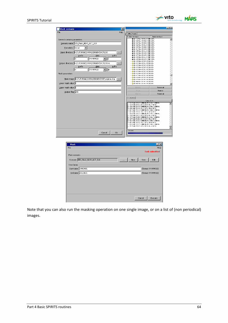
SPIRITS Tutorial


Note that you can also run the masking operation on one single image, or on a list of (non periodical) images.

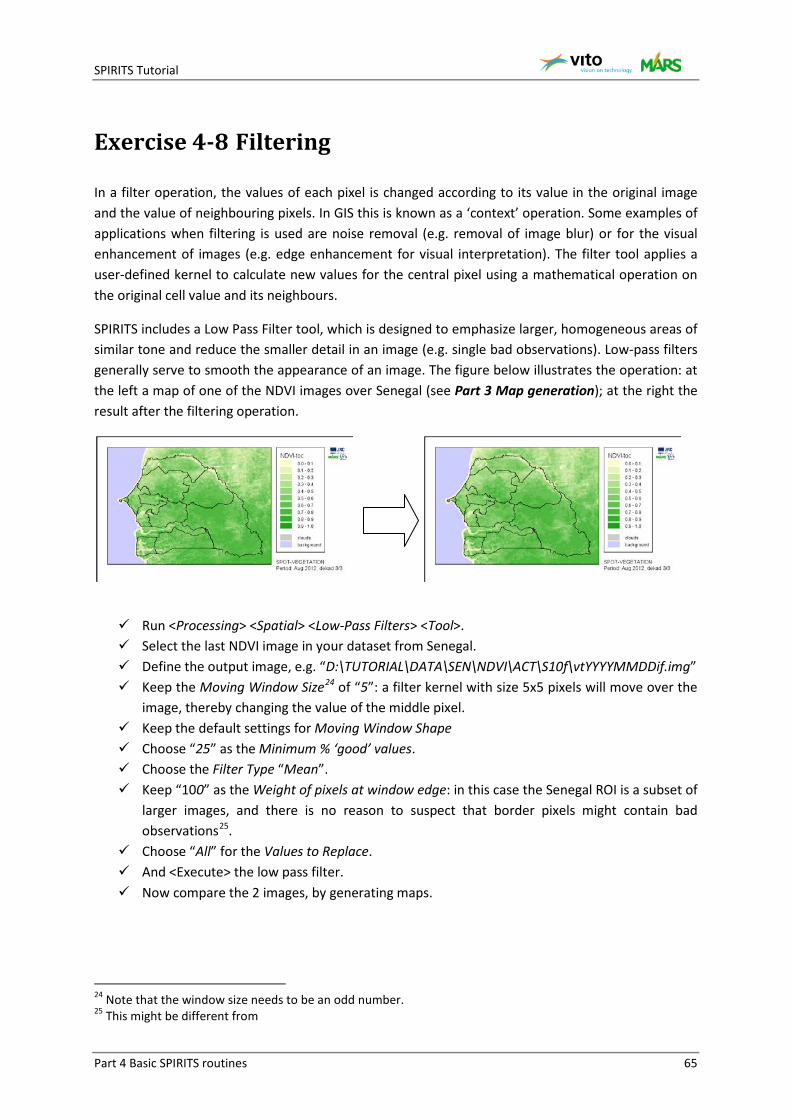
SPIRITS Tutorial


Exercise 4-8 Filtering

In a filter operation, the values of each pixel is changed according to its value in the original image and the value of neighbouring pixels. In GIS this is known as a ‘context’ operation. Some examples of applications when filtering is used are noise removal (e.g. removal of image blur) or for the visual enhancement of images (e.g. edge enhancement for visual interpretation). The filter tool applies a user-defined kernel to calculate new values for the central pixel using a mathematical operation on the original cell value and its neighbours.

SPIRITS includes a Low Pass Filter tool, which is designed to emphasize larger, homogeneous areas of similar tone and reduce the smaller detail in an image (e.g. single bad observations). Low-pass filters generally serve to smooth the appearance of an image. The figure below illustrates the operation: at the left a map of one of the NDVI images over Senegal (see Part 3 Map generation); at the right the result after the filtering operation.

Run <Processing> <Spatial> <Low-Pass Filters> <Tool>. Select the last NDVI image in your dataset from Senegal. Define the output image, e.g. “D:\TUTORIAL\DATA\SEN\NDVI\ACT\S10f\vtYYYYMMDDif.img” Keep the Moving Window Size24 of “5”: a filter kernel with size 5x5 pixels will move over the

image, thereby changing the value of the middle pixel. Keep the default settings for Moving Window Shape Choose “25” as the Minimum % ‘good’ values. Choose the Filter Type “Mean”. Keep “100” as the Weight of pixels at window edge: in this case the Senegal ROI is a subset of

larger images, and there is no reason to suspect that border pixels might contain bad observations25.

Choose “All” for the Values to Replace. And <Execute> the low pass filter. Now compare the 2 images, by generating maps.

24 Note that the window size needs to be an odd number. 25 This might be different from

SPIRITS Tutorial


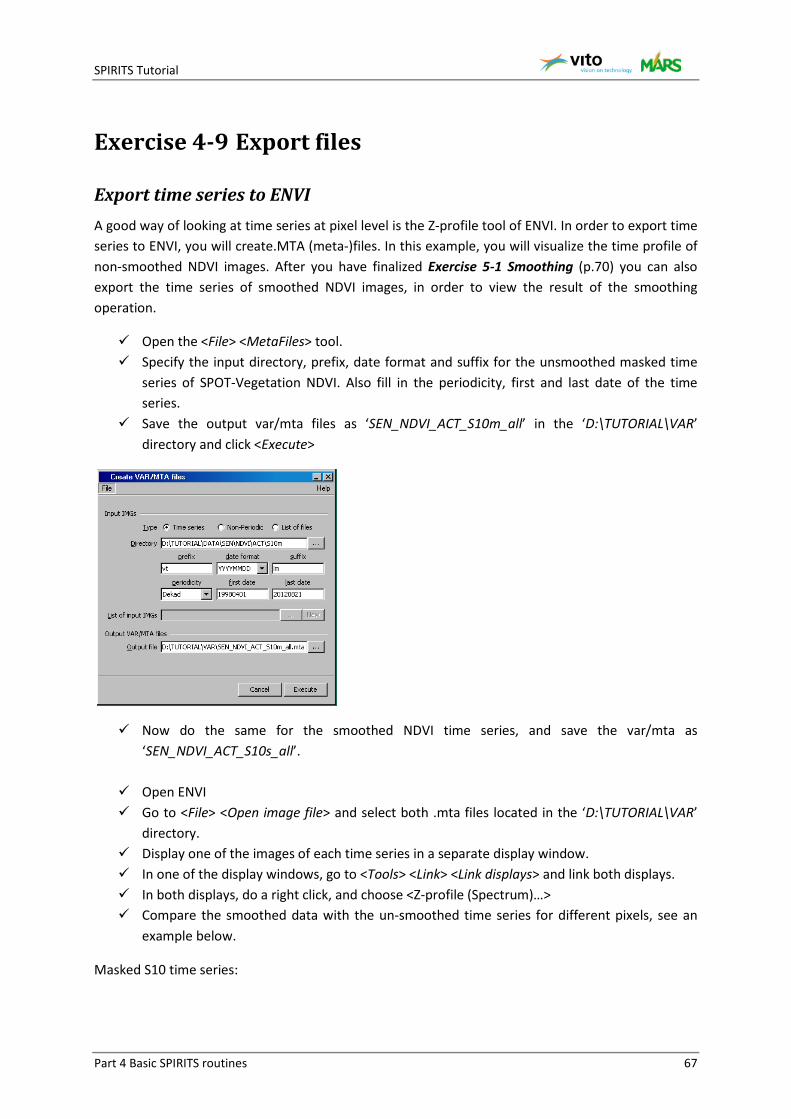
SPIRITS Tutorial


Exercise 4-9 Export files

Export time series to ENVI A good way of looking at time series at pixel level is the Z-profile tool of ENVI. In order to export time series to ENVI, you will create.MTA (meta-)files. In this example, you will visualize the time profile of non-smoothed NDVI images. After you have finalized Exercise 5-1 Smoothing (p.70) you can also export the time series of smoothed NDVI images, in order to view the result of the smoothing operation.

Open the <File> <MetaFiles> tool. Specify the input directory, prefix, date format and suffix for the unsmoothed masked time

series of SPOT-Vegetation NDVI. Also fill in the periodicity, first and last date of the time series.

Save the output var/mta files as ‘SEN_NDVI_ACT_S10m_all’ in the ‘D:\TUTORIAL\VAR’ directory and click <Execute>

Now do the same for the smoothed NDVI time series, and save the var/mta as ‘SEN_NDVI_ACT_S10s_all’.

Open ENVI Go to <File> <Open image file> and select both .mta files located in the ‘D:\TUTORIAL\VAR’

directory. Display one of the images of each time series in a separate display window. In one of the display windows, go to <Tools> <Link> <Link displays> and link both displays. In both displays, do a right click, and choose <Z-profile (Spectrum)…> Compare the smoothed data with the un-smoothed time series for different pixels, see an

example below.

Masked S10 time series:

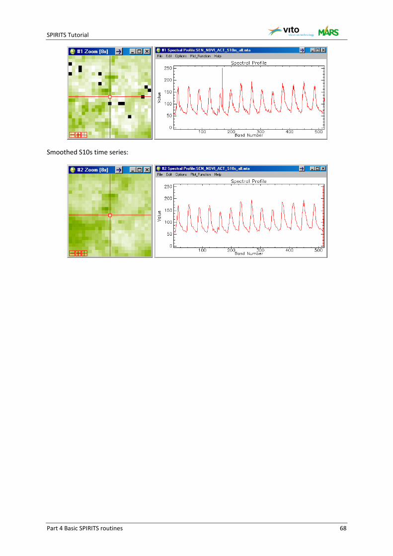
SPIRITS Tutorial


Smoothed S10s time series:

SPIRITS Tutorial

Part 5 Time Series Analysis in one season 69

Part 5 Time Series Analysis in one season

This part contains exercises on a series of analysis routines for time series analysis within one season or year:

• Exercise 5-1 Smoothing including an exercise on the temporal smoothing of S10 NDVI composites to S10s

• Exercise 5-2 Maximum Value Composites including an exercise on the maximum value compositing of S10s NDVI composites to S30

• Exercise 5-3 Mean Value Composites including an exercise on the mean value compositing of S10 RFE to S30 and the generation of total monthly RFE

• Exercise 5-4 Clustering including exercises on clustering actual NDVI values and vegetation anomalies


SPIRITS Tutorial


Exercise 5-1 Smoothing

Dekadal composite images (S10), such as S10 NDVI from SPOT-Vegetation often still contain a lot of perturbations. Below normal vegetation indicator may appear in regions where insufficient registrations are available for the maximum value compositing (MVC) process. Missing values occur for example in winter at higher latitudes. The most important source of noise however are clouds, because clouds often persist longer than 10 days. In temporal profiles, clouds can be recognized as irregular dips. These perturbations are sometimes so prevalent that they influence the analysis of the original composites. The simplest solution is to use a longer compositing period, and for instance create monthly instead of 10-daily MVC (see also Exercise 5-2 Maximum Value Composites), but this sacrifices temporal resolution. Therefore, several procedures were developed for ‘smoothing’ the 10-daily image series, based on Best Index Slope Extraction (BISE26) and based on a weighted least-squares approach developed by Swets et al27. In this exercise we use a modified Swets approach, as described by Klisch et al28.

The objective of this exercise is to apply temporal smoothing to an NDVI time series, in order to reduce the effect of clouds and atmospheric noise on decadal images.

Open the <Processing> <Temporal> <Smoothing> <Smooth> user interface.

! Smoothing is a complex operation which requires many parameters, but in this exercise you will use the default settings. For the explanation of all settings, see the SPIRITS Manual (click <Help> in the upper right corner of the ‘Smooth’ interface). The smooth dialogue windows includes the settings which are common to both methods. At the bottom you can choose between the VITO method (BISE) or JRC method (SWETS).

Define the input parameters: o The in-period runs from “19980401” till “20120821” and the input path is

‘D:\TUTORIAL\DATA\SEN\NDVI\ACT\S10m’. o The filename prefix is “vt”, date format is “YYYYMMDD”, and suffix is “im”. o Max. Missing (Centre): The maximum number of missing in-images are the maximum

number of consecutively missing actual images allowed in the centre of the time series. It is possible to replace missing images with interpolated values. If the input image time series is complete, this can be put to “0”.

o Replace missing IMGs at edges: ideally there should be images before the beginning and after the end of the input time series to allow smoothing of the first and last images. In the exercise you choose the simplest option (‘none’). It is possible to

26 Viovy, N., Arino, O., Belward, A., 1992. The best index slope extraction (BISE) : a method for reducing noise in NDVI time-series. International Journal of Remote Sensing, 13(8), 1585-1590. 27 Swets, D., Reed, B., Rowland, J., Marko, S., 1999. A weighted least-squares approach to temporal NDVI smoothing, ASPRS Annual Conference, Portland, Oregon, pp. 526-536. 28 Klisch, A., Royer, A., Lazar, C., Baruth, B., Genovese, G., 2006. Extraction of phenological parameters from temporally smoothed vegetation indices. ISPRS Archives XXXVI-8/W48 Workshop proceedings: Remote sensing support to crop yield forecast and area estimates.

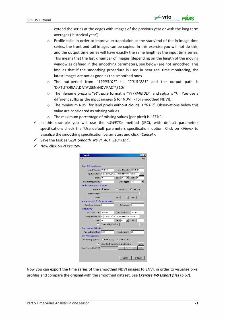
SPIRITS Tutorial


extend the series at the edges with images of the previous year or with the long term averages (‘historical year’).

o Profile tails: In order to improve extrapolation at the start/end of the in image time series, the front and tail images can be copied. In this exercise you will not do this, and the output time series will have exactly the same length as the input time series. This means that the last x number of images (depending on the length of the moving window as defined in the smoothing parameters, see below) are not smoothed. This implies that if the smoothing procedure is used in near real time monitoring, the latest images are not as good as the smoothed ones.

o The out-period from “19990101” till “20101221” and the output path is ‘D:\TUTORIAL\DATA\SEN\NDVI\ACT\S10s’.

o The filename prefix is “vt”, date format is “YYYYMMDD”, and suffix is “k”. You use a different suffix as the input images (i for NDVI, k for smoothed NDVI).

o The minimum NDVI for land pixels without clouds is “0.05”. Observations below this value are considered as missing values.

o The maximum percentage of missing values (per pixel) is “75%”. In this example you will use the <SWETS> method (JRC), with default parameters

specification: check the ‘Use default parameters specification’ option. Click on <View> to visualize the smoothing specification parameters and click <Cancel>.

Save the task as ‘SEN_Smooth_NDVI_ACT_S10m.tnt’. Now click on <Execute>.

Now you can export the time series of the smoothed NDVI images to ENVI, in order to visualize pixel profiles and compare the original with the smoothed dataset. See Exercise 4-9 Export files (p.67).

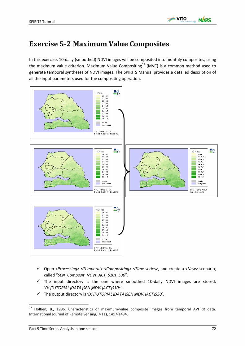
SPIRITS Tutorial


Exercise 5-2 Maximum Value Composites

In this exercise, 10-daily (smoothed) NDVI images will be composited into monthly composites, using the maximum value criterion. Maximum Value Compositing29 (MVC) is a common method used to generate temporal syntheses of NDVI images. The SPIRITS Manual provides a detailed description of all the input parameters used for the compositing operation.

Open <Processing> <Temporal> <Compositing> <Time series>, and create a <New> scenario, called “SEN_Composit_NDVI_ACT_S10s_S30”.

The input directory is the one where smoothed 10-daily NDVI images are stored: ‘D:\TUTORIAL\DATA\SEN\NDVI\ACT\S10s’.

The output directory is ‘D:\TUTORIAL\DATA\SEN\NDVI\ACT\S30’.

29 Holben, B., 1986. Characteristics of maximum-value composite images from temporal AVHRR data. International Journal of Remote Sensing, 7(11), 1417-1434.

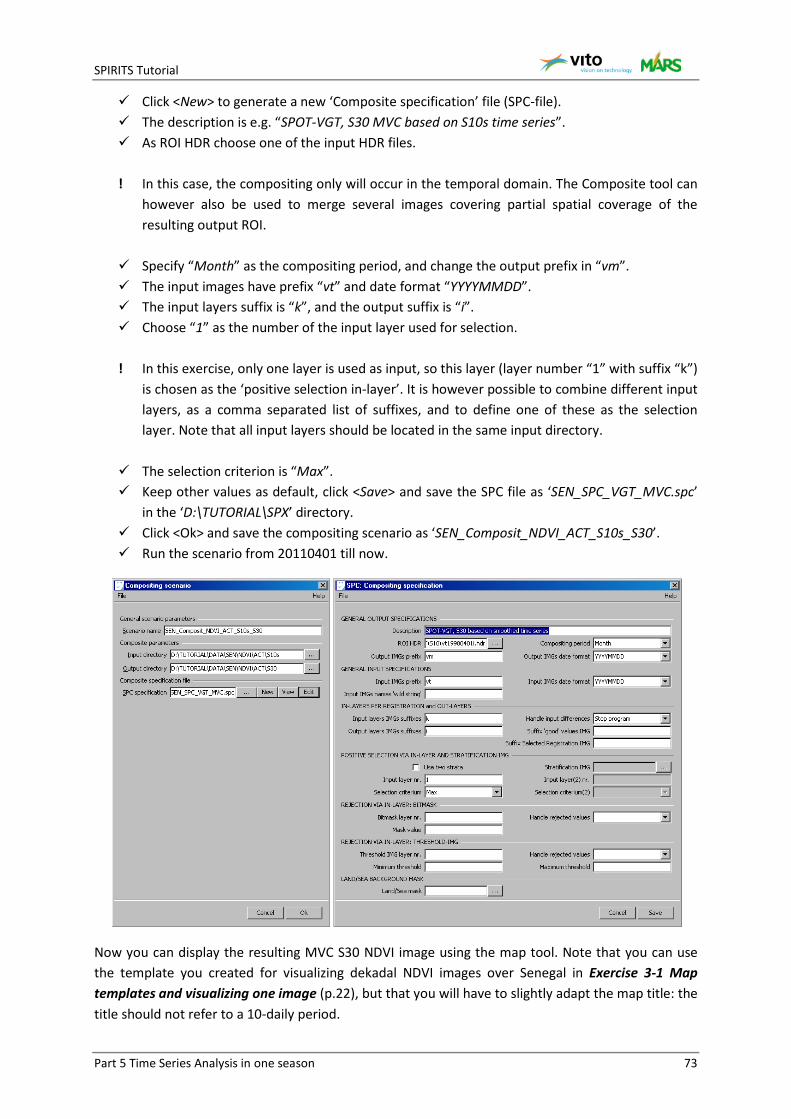
SPIRITS Tutorial


Click <New> to generate a new ‘Composite specification’ file (SPC-file). The description is e.g. “SPOT-VGT, S30 MVC based on S10s time series”. As ROI HDR choose one of the input HDR files.

! In this case, the compositing only will occur in the temporal domain. The Composite tool can

however also be used to merge several images covering partial spatial coverage of the resulting output ROI.

Specify “Month” as the compositing period, and change the output prefix in “vm”. The input images have prefix “vt” and date format “YYYYMMDD”. The input layers suffix is “k”, and the output suffix is “i”. Choose “1” as the number of the input layer used for selection.

! In this exercise, only one layer is used as input, so this layer (layer number “1” with suffix “k”)

is chosen as the ‘positive selection in-layer’. It is however possible to combine different input layers, as a comma separated list of suffixes, and to define one of these as the selection layer. Note that all input layers should be located in the same input directory.

The selection criterion is “Max”. Keep other values as default, click <Save> and save the SPC file as ‘SEN_SPC_VGT_MVC.spc’

in the ‘D:\TUTORIAL\SPX’ directory. Click <Ok> and save the compositing scenario as ‘SEN_Composit_NDVI_ACT_S10s_S30’. Run the scenario from 20110401 till now.

Now you can display the resulting MVC S30 NDVI image using the map tool. Note that you can use the template you created for visualizing dekadal NDVI images over Senegal in Exercise 3-1 Map templates and visualizing one image (p.22), but that you will have to slightly adapt the map title: the title should not refer to a 10-daily period.

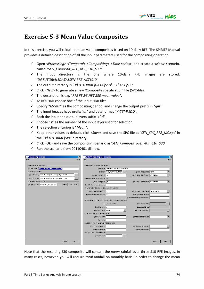
SPIRITS Tutorial


Exercise 5-3 Mean Value Composites

In this exercise, you will calculate mean value composites based on 10-daily RFE. The SPIRITS Manual provides a detailed description of all the input parameters used for the compositing operation.

Open <Processing> <Temporal> <Compositing> <Time series>, and create a <New> scenario, called “SEN_Composit_RFE_ACT_S10_S30”.

The input directory is the one where 10-daily RFE images are stored: ‘D:\TUTORIAL\DATA\SEN\RFE\ACT\S10’.

The output directory is ‘D:\TUTORIAL\DATA\SEN\RFE\ACT\S30’. Click <New> to generate a new ‘Composite specification’ file (SPC-file). The description is e.g. “RFE FEWS NET S30 mean value”. As ROI HDR choose one of the input HDR files. Specify “Month” as the compositing period, and change the output prefix in “gm”. The input images have prefix “gt” and date format “YYYYMMDD”. Both the input and output layers suffix is “rf”. Choose “1” as the number of the input layer used for selection. The selection criterion is “Mean”. Keep other values as default, click <Save> and save the SPC file as ‘SEN_SPC_RFE_MC.spc’ in

the ‘D:\TUTORIAL\SPX’ directory. Click <Ok> and save the compositing scenario as ‘SEN_Composit_RFE_ACT_S10_S30’. Run the scenario from 20110401 till now.

Note that the resulting S30 composite will contain the mean rainfall over three S10 RFE images. In many cases, however, you will require total rainfall on monthly basis. In order to change the mean

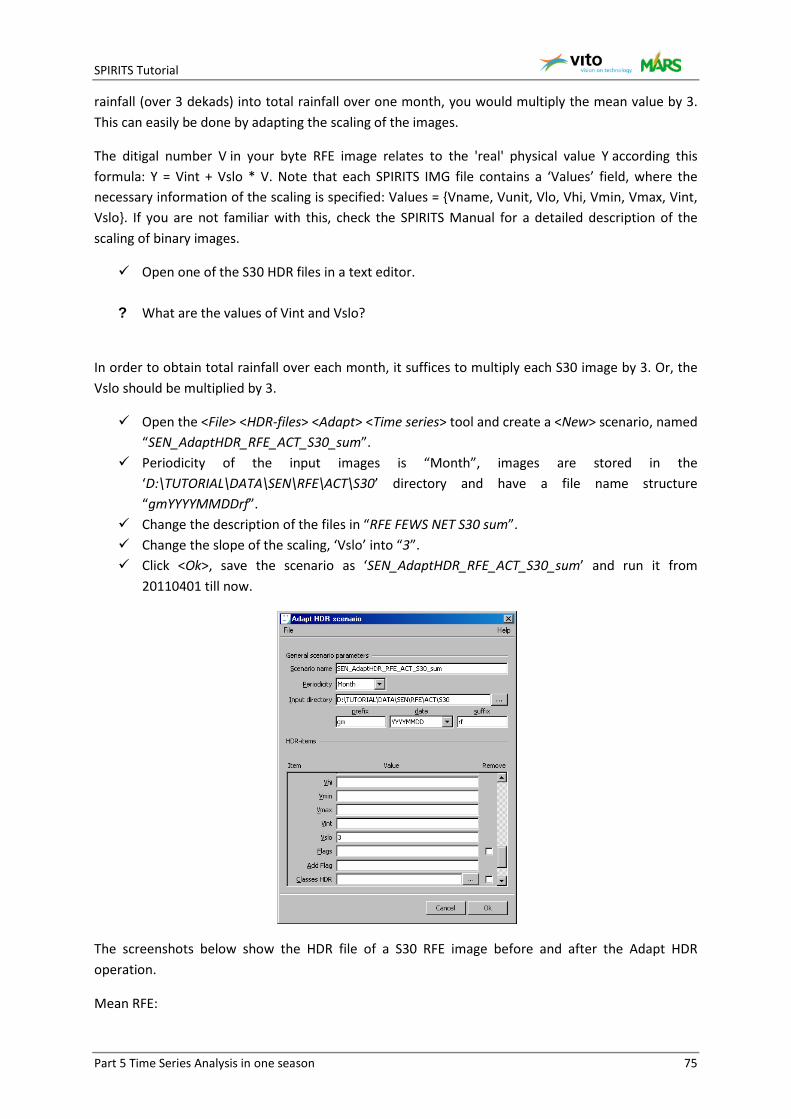
SPIRITS Tutorial


rainfall (over 3 dekads) into total rainfall over one month, you would multiply the mean value by 3. This can easily be done by adapting the scaling of the images.

The ditigal number V in your byte RFE image relates to the 'real' physical value Y according this formula: Y = Vint + Vslo * V. Note that each SPIRITS IMG file contains a ‘Values’ field, where the necessary information of the scaling is specified: Values = {Vname, Vunit, Vlo, Vhi, Vmin, Vmax, Vint, Vslo}. If you are not familiar with this, check the SPIRITS Manual for a detailed description of the scaling of binary images.

Open one of the S30 HDR files in a text editor.

? What are the values of Vint and Vslo?

In order to obtain total rainfall over each month, it suffices to multiply each S30 image by 3. Or, the Vslo should be multiplied by 3.

Open the <File> <HDR-files> <Adapt> <Time series> tool and create a <New> scenario, named “SEN_AdaptHDR_RFE_ACT_S30_sum”.

Periodicity of the input images is “Month”, images are stored in the ‘D:\TUTORIAL\DATA\SEN\RFE\ACT\S30’ directory and have a file name structure “gmYYYYMMDDrf”.

Change the description of the files in “RFE FEWS NET S30 sum”. Change the slope of the scaling, ‘Vslo’ into “3”. Click <Ok>, save the scenario as ‘SEN_AdaptHDR_RFE_ACT_S30_sum’ and run it from

20110401 till now.

The screenshots below show the HDR file of a S30 RFE image before and after the Adapt HDR operation.

Mean RFE:

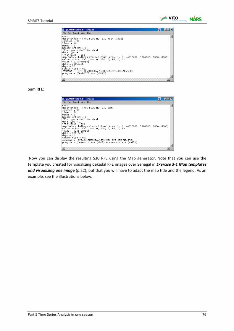
SPIRITS Tutorial


Sum RFE:

Now you can display the resulting S30 RFE using the Map generator. Note that you can use the template you created for visualizing dekadal RFE images over Senegal in Exercise 3-1 Map templates and visualizing one image (p.22), but that you will have to adapt the map title and the legend. As an example, see the illustrations below.

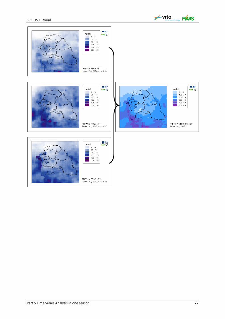
SPIRITS Tutorial


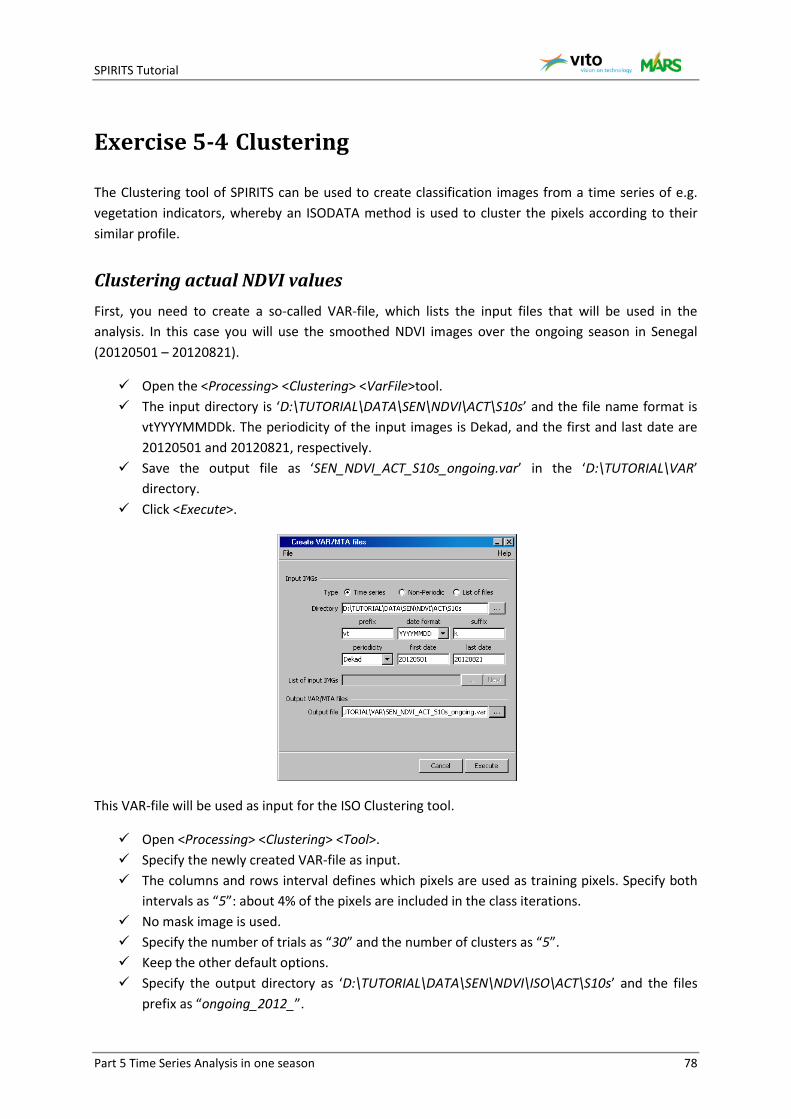
SPIRITS Tutorial


Exercise 5-4 Clustering

The Clustering tool of SPIRITS can be used to create classification images from a time series of e.g. vegetation indicators, whereby an ISODATA method is used to cluster the pixels according to their similar profile.

Clustering actual NDVI values First, you need to create a so-called VAR-file, which lists the input files that will be used in the analysis. In this case you will use the smoothed NDVI images over the ongoing season in Senegal (20120501 – 20120821).

Open the <Processing> <Clustering> <VarFile>tool. The input directory is ‘D:\TUTORIAL\DATA\SEN\NDVI\ACT\S10s’ and the file name format is

vtYYYYMMDDk. The periodicity of the input images is Dekad, and the first and last date are 20120501 and 20120821, respectively.

Save the output file as ‘SEN_NDVI_ACT_S10s_ongoing.var’ in the ‘D:\TUTORIAL\VAR’ directory.

Click <Execute>.

This VAR-file will be used as input for the ISO Clustering tool.

Open <Processing> <Clustering> <Tool>. Specify the newly created VAR-file as input. The columns and rows interval defines which pixels are used as training pixels. Specify both

intervals as “5”: about 4% of the pixels are included in the class iterations. No mask image is used. Specify the number of trials as “30” and the number of clusters as “5”. Keep the other default options. Specify the output directory as ‘D:\TUTORIAL\DATA\SEN\NDVI\ISO\ACT\S10s’ and the files

prefix as “ongoing_2012_”.

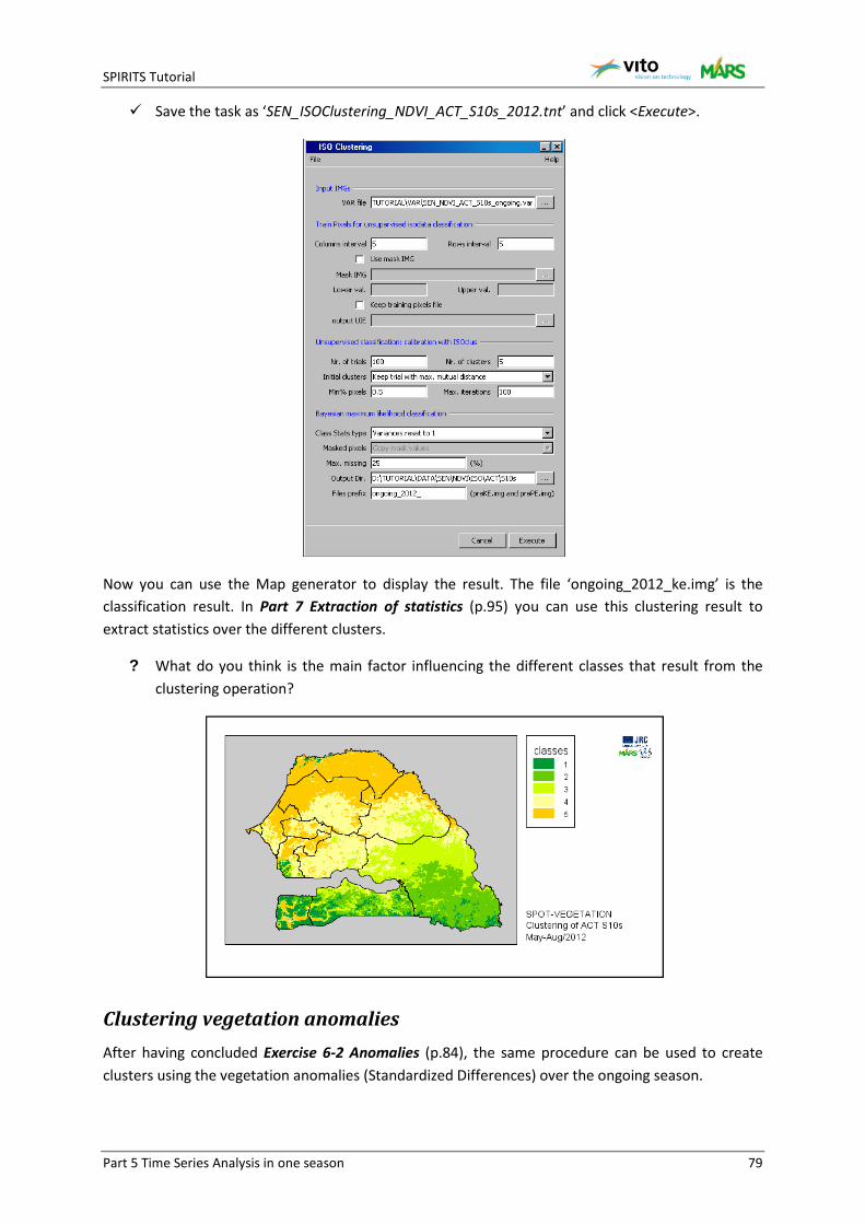
SPIRITS Tutorial


Save the task as ‘SEN_ISOClustering_NDVI_ACT_S10s_2012.tnt’ and click <Execute>.

Now you can use the Map generator to display the result. The file ‘ongoing_2012_ke.img’ is the classification result. In Part 7 Extraction of statistics (p.95) you can use this clustering result to extract statistics over the different clusters.

? What do you think is the main factor influencing the different classes that result from the clustering operation?

Clustering vegetation anomalies After having concluded Exercise 6-2 Anomalies (p.84), the same procedure can be used to create clusters using the vegetation anomalies (Standardized Differences) over the ongoing season.

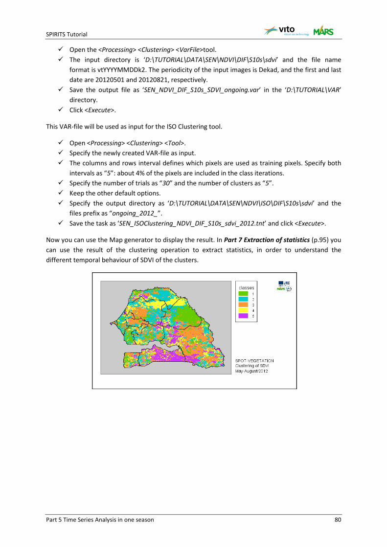
SPIRITS Tutorial


Open the <Processing> <Clustering> <VarFile>tool. The input directory is ‘D:\TUTORIAL\DATA\SEN\NDVI\DIF\S10s\sdvi’ and the file name

format is vtYYYYMMDDk2. The periodicity of the input images is Dekad, and the first and last date are 20120501 and 20120821, respectively.

Save the output file as ‘SEN_NDVI_DIF_S10s_SDVI_ongoing.var’ in the ‘D:\TUTORIAL\VAR’ directory.

Click <Execute>.

This VAR-file will be used as input for the ISO Clustering tool.

Open <Processing> <Clustering> <Tool>. Specify the newly created VAR-file as input. The columns and rows interval defines which pixels are used as training pixels. Specify both

intervals as “5”: about 4% of the pixels are included in the class iterations. Specify the number of trials as “30” and the number of clusters as “5”. Keep the other default options. Specify the output directory as ‘D:\TUTORIAL\DATA\SEN\NDVI\ISO\DIF\S10s\sdvi’ and the

files prefix as “ongoing_2012_”. Save the task as ‘SEN_ISOClustering_NDVI_DIF_S10s_sdvi_2012.tnt’ and click <Execute>.

Now you can use the Map generator to display the result. In Part 7 Extraction of statistics (p.95) you can use the result of the clustering operation to extract statistics, in order to understand the different temporal behaviour of SDVI of the clusters.

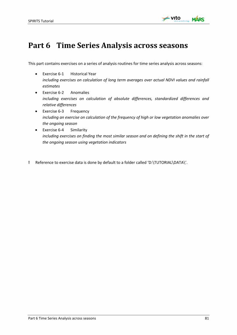
SPIRITS Tutorial

Part 6 Time Series Analysis across seasons 81

Part 6 Time Series Analysis across seasons

This part contains exercises on a series of analysis routines for time series analysis across seasons:

• Exercise 6-1 Historical Year including exercises on calculation of long term averages over actual NDVI values and rainfall estimates

• Exercise 6-2 Anomalies including exercises on calculation of absolute differences, standardized differences and relative differences

• Exercise 6-3 Frequency including an exercise on calculation of the frequency of high or low vegetation anomalies over the ongoing season

• Exercise 6-4 Similarity including exercises on finding the most similar season and on defining the shift in the start of the ongoing season using vegetation indicators


SPIRITS Tutorial


Exercise 6-1 Historical Year

The objective of this exercise is to create a series of images with the long term average (LTA) for each dekad of the year. This is generally needed for all the operations which compute anomalies, comparing the actual state with the long term average, such as difference images or seasonal profiles.

! We commonly use the definition “historical year” to define the long term average images for a time series. It is often useful in crop monitoring is to compare the current season with previous reference situations. Therefore, we want to compute the historical year based on data from the beginning of the time series to right before the start of the current season. The current season should not be included in the long term average and the long term average is normally updated at the beginning of each agricultural year. However, this depends of the goal of each application.

Calculation of the ‘historical year’ for NDVI Go to the <Processing> <Temporal> <Long-term statistics > tool. Define the input image path, filename and date and periodicity as usual. (If necessary, check

the filename-structure in the ‘D:\TUTORIAL\DATA\SEN\NDVI\ACT\S10’.) Set the beginning year as the first full year of the time series (“1999” in case of SPOT

VEGETATION), and choose the year preceding the current agricultural season as the end year. In this case, you will consider “2012” as the ongoing season, thus you calculate the historical year based on decadal images from the beginning of 1999 till the end of 2011.

The output should be saved in the ‘HIS’ directory at ‘D:\TUTORIAL\DATA\SEN\NDVI\HIS\S10s’.

The structure of the output file names can be identical to the input. Define a start and end period during the year (in MMDD format). This can be the whole year

(“0101” – “1221”), but could also be a subset of the year, for example only the months of the typical crop cycle.

Choose the type of output images. The most important are the Mean image, the Standard Deviation, Minimum and Maximum.

If you want to save the task file, click <File> <Save> and save the “SEN_LTA_NDVI_HIS_S10s.tnt” in the TNT folder.

Click <Execute>

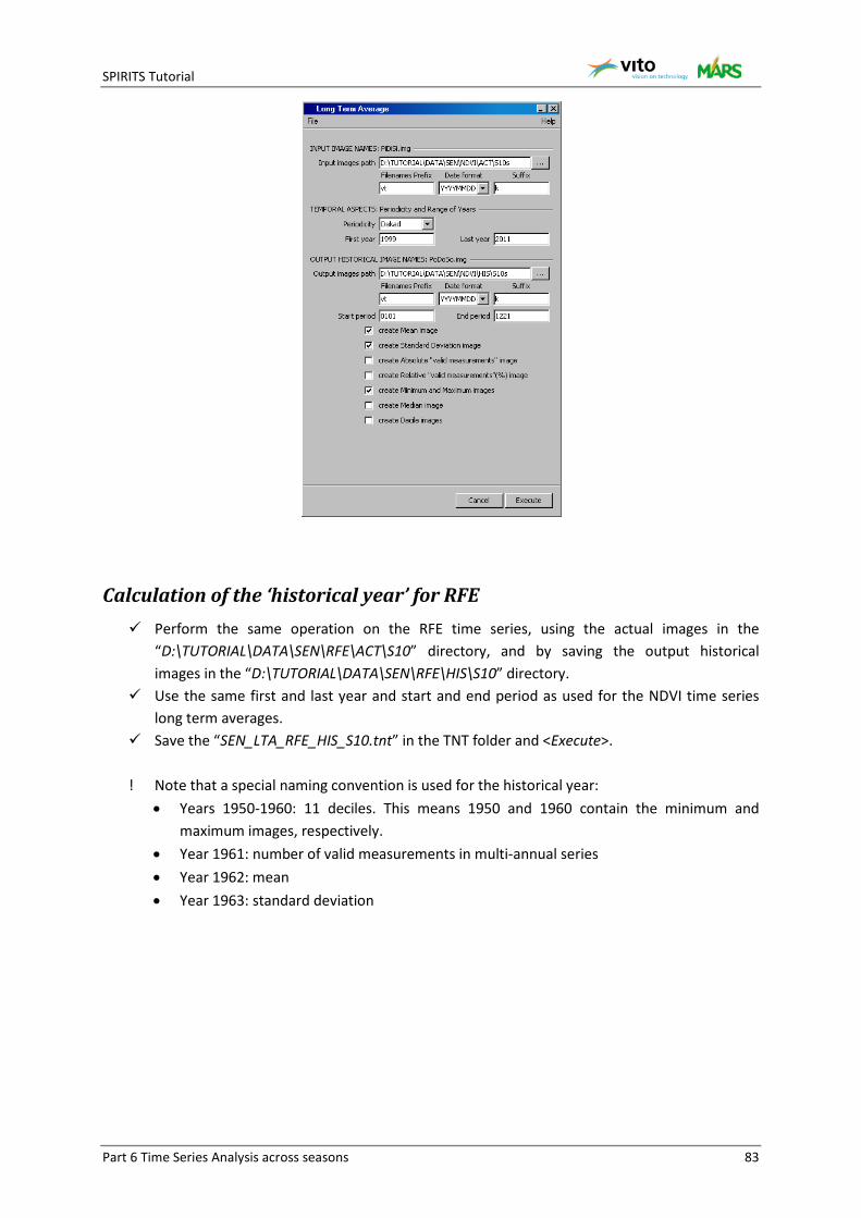
SPIRITS Tutorial


Calculation of the ‘historical year’ for RFE Perform the same operation on the RFE time series, using the actual images in the

“D:\TUTORIAL\DATA\SEN\RFE\ACT\S10” directory, and by saving the output historical images in the “D:\TUTORIAL\DATA\SEN\RFE\HIS\S10” directory.

Use the same first and last year and start and end period as used for the NDVI time series long term averages.

Save the “SEN_LTA_RFE_HIS_S10.tnt” in the TNT folder and <Execute>.

! Note that a special naming convention is used for the historical year: • Years 1950-1960: 11 deciles. This means 1950 and 1960 contain the minimum and

maximum images, respectively. • Year 1961: number of valid measurements in multi-annual series • Year 1962: mean • Year 1963: standard deviation

SPIRITS Tutorial


Exercise 6-2 Anomalies

In this exercise you will create vegetation anomaly maps based on the comparison of actual NDVI and RFE maps with the historical year.

! In the calculation of anomalies, the current dekad (or month or season) is compared to a certain reference situation. This reference situation can be the long term average (LTA), the previous year or a particularly good or bad year.

! Many different anomaly algorithms exist, all optimized for particular indicators and environments. Check the SPIRITS Manual for more information on available difference operators.

In this exercise you start with some basic anomaly indicators, comparing the actual situation with the long term average calculated in Exercise 6-1 Historical Year. How to visualize the output of the anomalies operation using the Map generator of SPIRITS is shown in Exercise 3-1 Map templates and visualizing one image.

Absolute differences The absolute difference is calculated as: ADVIy,p = Xy,p – meanp, with y = the year, and p = the period in the year (dekad).

Open <Processing> <Temporal> <Anomalies> <Time series>. You can create a new difference scenario, and run it on a series of input images. Click on

<New>. The first Scenario name is ‘SEN_ADVI_NDVI_ACT_S10s’. The Difference operator is the “AbsDif to historical average” (= ADVI, Absolute Difference

Vegetation Index). The Periodicity of the input and output is “Dekad”. The input images are the smoothed S10s NDVI images of Senegal, with prefix “vt”, date

format “YYYYMMDD” and suffix “k”. In Flags choose “UNI-Flagged”.

! Check the input image headers by opening one of them in a text editor, or by using the <View

HDR> operation. In this case the input flag values are: 251=missing, 252=cloud, 253=snow, 254=sea, 255=back, 254=back. By checking this option, also the output images will have the same flag values.

The reference images time series is the historical year (LTA, long term average). This is the result of the previous exercise Exercise 6-1 Historical Year.

! In case the LTA is not available, or in case you want to use a long term average different from the existing one, it can be done by checking the “calculate new” option. Note that in this case the computing time will increase significantly.

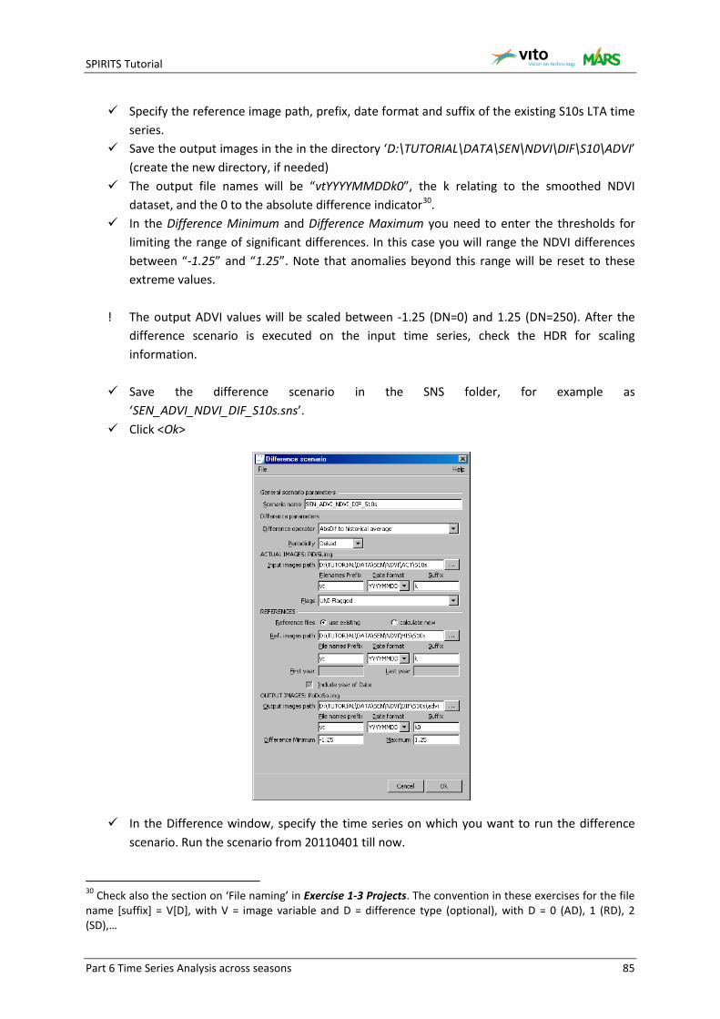
SPIRITS Tutorial


Specify the reference image path, prefix, date format and suffix of the existing S10s LTA time

series. Save the output images in the in the directory ‘D:\TUTORIAL\DATA\SEN\NDVI\DIF\S10\ADVI’

(create the new directory, if needed) The output file names will be “vtYYYYMMDDk0”, the k relating to the smoothed NDVI

dataset, and the 0 to the absolute difference indicator30. In the Difference Minimum and Difference Maximum you need to enter the thresholds for

limiting the range of significant differences. In this case you will range the NDVI differences between “-1.25” and “1.25”. Note that anomalies beyond this range will be reset to these extreme values.

! The output ADVI values will be scaled between -1.25 (DN=0) and 1.25 (DN=250). After the difference scenario is executed on the input time series, check the HDR for scaling information.

Save the difference scenario in the SNS folder, for example as ‘SEN_ADVI_NDVI_DIF_S10s.sns’.

Click <Ok>

In the Difference window, specify the time series on which you want to run the difference scenario. Run the scenario from 20110401 till now.

30 Check also the section on ‘File naming’ in Exercise 1-3 Projects. The convention in these exercises for the file name [suffix] = V[D], with V = image variable and D = difference type (optional), with D = 0 (AD), 1 (RD), 2 (SD),…

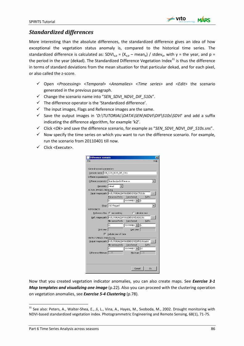
SPIRITS Tutorial


Standardized differences More interesting than the absolute differences, the standardized difference gives an idea of how exceptional the vegetation status anomaly is, compared to the historical time series. The standardized difference is calculated as: SDVIy,p = (Xy,p – meanp) / stdevp, with y = the year, and p = the period in the year (dekad). The Standardized Difference Vegetation Index31 is thus the difference in terms of standard deviations from the mean situation for that particular dekad, and for each pixel, or also called the z-score.

Open <Processing> <Temporal> <Anomalies> <Time series> and <Edit> the scenario generated in the previous paragraph.

Change the scenario name into “SEN_SDVI_NDVI_DIF_S10s”. The difference operator is the ‘Standardized difference’. The input images, Flags and Reference images are the same. Save the output images in ‘D:\TUTORIAL\DATA\SEN\NDVI\DIF\S10s\SDVI’ and add a suffix

indicating the difference algorithm, for example ‘k2’. Click <Ok> and save the difference scenario, for example as “SEN_SDVI_NDVI_DIF_S10s.sns”. Now specify the time series on which you want to run the difference scenario. For example,

run the scenario from 20110401 till now. Click <Execute>.

Now that you created vegetation indicator anomalies, you can also create maps. See Exercise 3-1 Map templates and visualizing one image (p.22). Also you can proceed with the clustering operation on vegetation anomalies, see Exercise 5-4 Clustering (p.78).

31 See also: Peters, A., Walter-Shea, E., Ji, L., Vina, A., Hayes, M., Svoboda, M., 2002. Drought monitoring with NDVI-based standardized vegetation index. Photogrammetric Engineering and Remote Sensing, 68(1), 71-75.

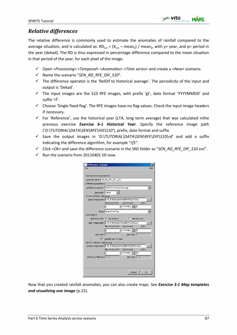
SPIRITS Tutorial


Relative differences The relative difference is commonly used to estimate the anomalies of rainfall compared to the average situation, and is calculated as: RDy,p = (Xy,p – meanp) / meanp, with y= year, and p= period in the year (dekad). The RD is thus expressed in percentage difference compared to the mean situation in that period of the year, for each pixel of the image.

Open <Processing> <Temporal> <Anomalies> <Time series> and create a <New> scenario. Name the scenario “SEN_RD_RFE_DIF_S10”. The difference operator is the ‘RelDif to historical average’. The periodicity of the input and

output is ‘Dekad’. The input images are the S10 RFE images, with prefix ‘gt’, date format ‘YYYYMMDD’ and

suffix ‘rf’. Choose ‘Single fixed flag’. The RFE images have no flag values. Check the input image headers

if necessary. For ‘Reference’, use the historical year (LTA, long term average) that was calculated inthe

previous exercise Exercise 6-1 Historical Year. Specify the reference image path (‘D:\TUTORIAL\DATA\SEN\RFE\HIS\S10’), prefix, date format and suffix.

Save the output images in ‘D:\TUTORIAL\DATA\SEN\RFE\DIF\S10\rd’ and add a suffix indicating the difference algorithm, for example “rf1”.

Click <Ok> and save the difference scenario in the SNS folder as “SEN_RD_RFE_DIF_S10.sns”. Run the scenario from 20110401 till now.

Now that you created rainfall anomalies, you can also create maps. See Exercise 3-1 Map templates and visualizing one image (p.22).

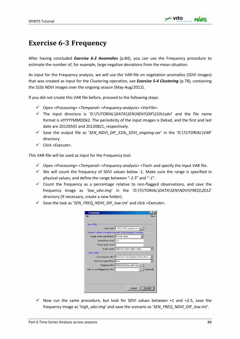
SPIRITS Tutorial


Exercise 6-3 Frequency

After having concluded Exercise 6-2 Anomalies (p.84), you can use the Frequency procedure to estimate the number of, for example, large negative deviations from the mean situation.

As input for the Frequency analysis, we will use the VAR-file on vegetation anomalies (SDVI images) that was created as input for the Clustering operation, see Exercise 5-4 Clustering (p.78), containing the S10s NDVI images over the ongoing season (May-Aug/2012).

If you did not create this VAR file before, proceed to the following steps:

Open <Processing> <Temporal> <Frequency analysis> <VarFile>. The input directory is ‘D:\TUTORIAL\DATA\SEN\NDVI\DIF\S10s\sdvi’ and the file name

format is vtYYYYMMDDk2. The periodicity of the input images is Dekad, and the first and last date are 20120501 and 20120821, respectively.

Save the output file as ‘SEN_NDVI_DIF_S10s_SDVI_ongoing.var’ in the ‘D:\TUTORIAL\VAR’ directory.

Click <Execute>.

This VAR-file will be used as input for the Frequency tool.

Open <Processing> <Temporal> <Frequency analysis> <Tool> and specify the input VAR file. We will count the frequency of SDVI values below -1. Make sure the range is specified in

physical values, and define the range between “-2.5” and “-1”. Count the frequency as a percentage relative to non-flagged observations, and save the

frequency image as ‘low_sdvi.img’ in the ‘D:\TUTORIAL\DATA\SEN\NDVI\FREQ\2012’ directory (if necessary, create a new folder).

Save the task as ‘SEN_FREQ_NDVI_DIF_low.tnt’ and click <Execute>.

Now run the same procedure, but look for SDVI values between +1 and +2.5, save the frequency image as ‘high_sdvi.img’ and save the scenario as ‘SEN_FREQ_NDVI_DIF_low.tnt’.

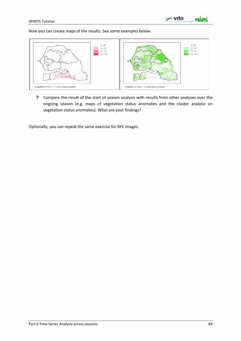
SPIRITS Tutorial


Now you can create maps of the results. See some examples below.

? Compare the result of the start of season analysis with results from other analyses over the ongoing season (e.g. maps of vegetation status anomalies and the cluster analysis on vegetation status anomalies). What are your findings?

Optionally, you can repeat the same exercise for RFE images.

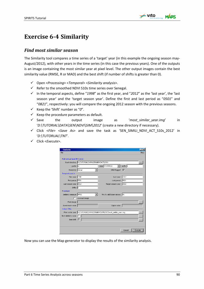
SPIRITS Tutorial


Exercise 6-4 Similarity

Find most similar season The Similarity tool compares a time series of a ‘target’ year (in this example the ongoing season may-August/2012), with other years in the time series (in this case the previous years). One of the outputs is an image containing the most similar year at pixel level. The other output images contain the best similarity value (RMSE, R or MAD) and the best shift (if number of shifts is greater than 0).

Open <Processing> <Temporal> <Similarity analysis>. Refer to the smoothed NDVI S10s time series over Senegal. In the temporal aspects, define “1998” as the first year, and “2012” as the ‘last year’, the ‘last

season year’ and the ‘target season year’. Define the first and last period as “0501” and “0821”, respectively: you will compare the ongoing 2012 season with the previous seasons.

Keep the ‘Shift’ number as “0”. Keep the procedure parameters as default. Save the output image as ‘most_similar_year.img’ in

‘D:\TUTORIAL\DATA\SEN\NDVI\SIM\2012’ (create a new directory if necessary). Click <File> <Save As> and save the task as ‘SEN_SIMILI_NDVI_ACT_S10s_2012’ in

‘D:\TUTORUAL\TNT’. Click <Execute>.

Now you can use the Map generator to display the results of the similarity analysis.

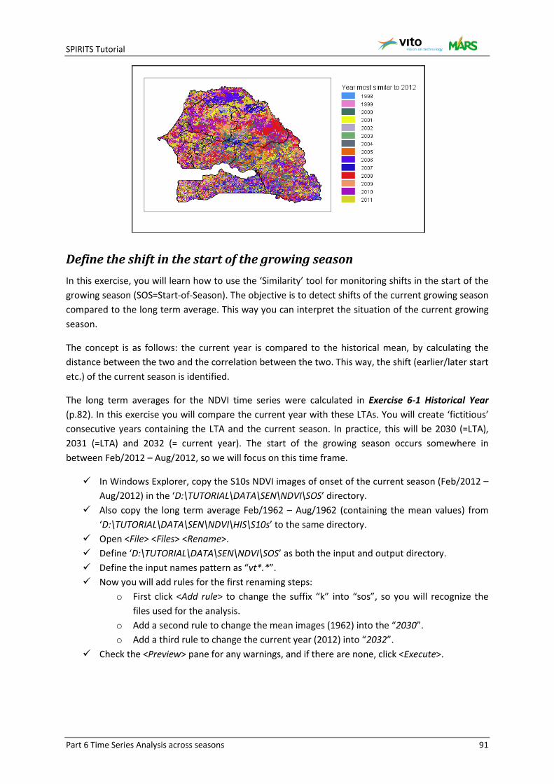
SPIRITS Tutorial


Define the shift in the start of the growing season In this exercise, you will learn how to use the ‘Similarity’ tool for monitoring shifts in the start of the growing season (SOS=Start-of-Season). The objective is to detect shifts of the current growing season compared to the long term average. This way you can interpret the situation of the current growing season.

The concept is as follows: the current year is compared to the historical mean, by calculating the distance between the two and the correlation between the two. This way, the shift (earlier/later start etc.) of the current season is identified.

The long term averages for the NDVI time series were calculated in Exercise 6-1 Historical Year (p.82). In this exercise you will compare the current year with these LTAs. You will create ‘fictitious’ consecutive years containing the LTA and the current season. In practice, this will be 2030 (=LTA), 2031 (=LTA) and 2032 (= current year). The start of the growing season occurs somewhere in between Feb/2012 – Aug/2012, so we will focus on this time frame.

In Windows Explorer, copy the S10s NDVI images of onset of the current season (Feb/2012 – Aug/2012) in the ‘D:\TUTORIAL\DATA\SEN\NDVI\SOS’ directory.

Also copy the long term average Feb/1962 – Aug/1962 (containing the mean values) from ‘D:\TUTORIAL\DATA\SEN\NDVI\HIS\S10s’ to the same directory.

Open <File> <Files> <Rename>. Define ‘D:\TUTORIAL\DATA\SEN\NDVI\SOS’ as both the input and output directory. Define the input names pattern as “vt*.*”. Now you will add rules for the first renaming steps:

o First click <Add rule> to change the suffix “k” into “sos”, so you will recognize the files used for the analysis.

o Add a second rule to change the mean images (1962) into the “2030”. o Add a third rule to change the current year (2012) into “2032”.

Check the <Preview> pane for any warnings, and if there are none, click <Execute>.

SPIRITS Tutorial


If you check the ‘D:\TUTORIAL\DATA\SEN\NDVI\SOS’ directory, you will notice how the SOS time series already contains the years 2030 (=LTA) and 2032 (=current year).

Go back to the <Rename> tool. Change the input names pattern into “vt1962*.*” and the output pattern into “vt2031%0.%1”. Check for warnings and click <Execute>.

Now the SOS time series contains 2030 (=LTA), 2031 (=LTA) and 2032 (=current year).

SPIRITS Tutorial


Note that SPIRITS, when performing operations, reads information from the image HDR files. In this case, changing the filenames into the years 2030-2032 is not enough, and also the ‘date’ field in the HDR needs to be adapted

Go to <File> <HDR-files> <Adapt> <Time series> and create a new scenario called “SEN_AdaptHDR_NDVI_SOS”.

Define the input directory, periodicity, file prefix, date format and suffix (“sos”). At the bottom of the HDR-times list, check the option to deduce the date field from the time

series filenames. Click <Ok> and save the scenario as ‘SEN_AdaptHDR_NDVI_SOS.sns’. Run the scenario for 20300201 till 20320821.

Now the dataset is ready for the shift analysis.

Open <Processing> <Temporal> <Similarity analysis>. Define the input images path, prefix, date format and suffix. In the temporal aspects, define “2030” as the first year, and “2032” as the ‘last year’, the ‘last

season year’ and the ‘target season year’. Define the first and last period as “0201” and “0821”, respectively.

Change the ‘Shifts’ number in “3”: we will look at shifts up to three dekads in both directions. Keep the procedure parameters as default. Save the output images as ‘most_similar_year.img’, ‘best_value.img’ and ‘best_shift.img’ in

‘D:\TUTORIAL\DATA\SEN\NDVI\SOS’. Click <File> <Save As> and save the task as ‘SEN_SIMILI_SOS.tnt’ in ‘D:\TUTORUAL\TNT’. Click <Execute>.

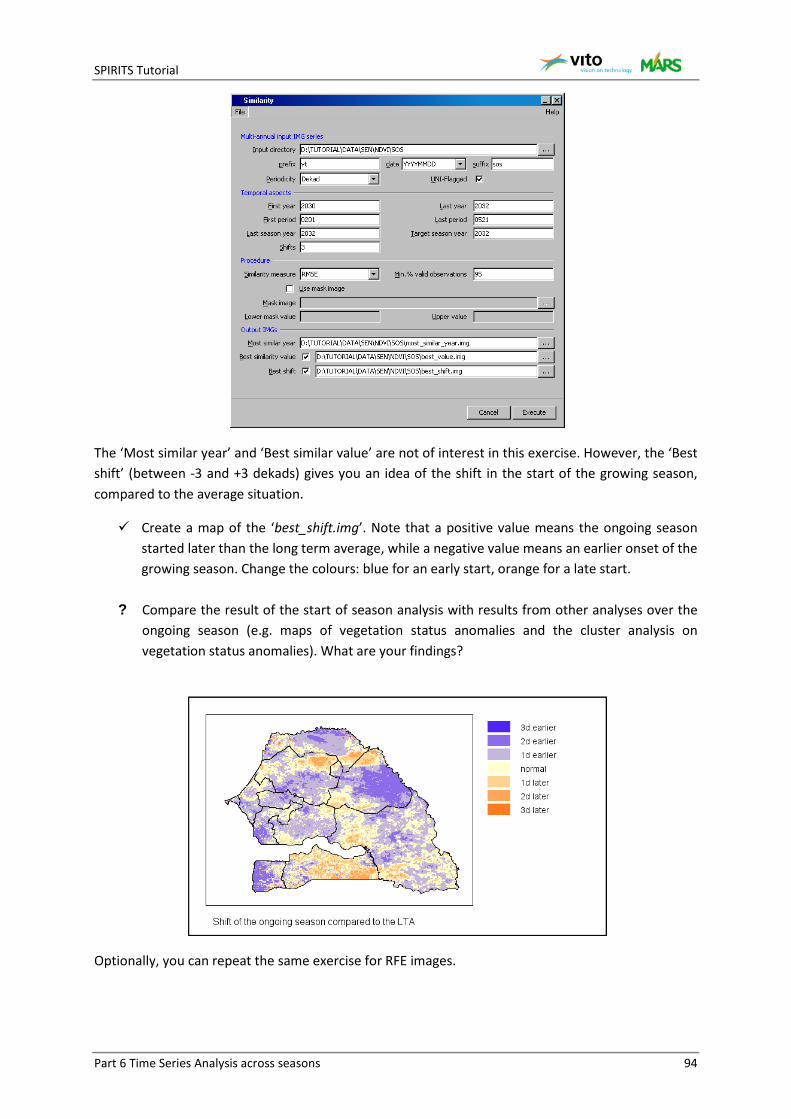
SPIRITS Tutorial


The ‘Most similar year’ and ‘Best similar value’ are not of interest in this exercise. However, the ‘Best shift’ (between -3 and +3 dekads) gives you an idea of the shift in the start of the growing season, compared to the average situation.

Create a map of the ‘best_shift.img’. Note that a positive value means the ongoing season started later than the long term average, while a negative value means an earlier onset of the growing season. Change the colours: blue for an early start, orange for a late start.

? Compare the result of the start of season analysis with results from other analyses over the

ongoing season (e.g. maps of vegetation status anomalies and the cluster analysis on vegetation status anomalies). What are your findings?

Optionally, you can repeat the same exercise for RFE images.

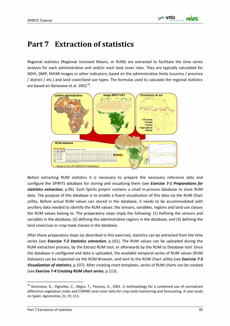
SPIRITS Tutorial

Part 7 Extraction of statistics 95

Part 7 Extraction of statistics

Regional statistics (Regional Unmixed Means, or RUM) are extracted to facilitate the time series analysis for each administrative unit and/or each land cover class. They are typically calculated for NDVI, DMP, fAPAR images or other indicators, based on the administrative limits (country / province / district / etc.) and land cover/land use types. The formulas used to calculate the regional statistics are based on Genovese et al. 200132.

Before extracting RUM statistics it is necessary to prepare the necessary reference data and configure the SPIRITS database for storing and visualizing them (see Exercise 7-1 Preparations for statistics extraction, p.96). Each Spirits project contains a small in-process database to store RUM data. The purpose of this database is to enable a fluent visualization of this data via the RUM Chart utility. Before actual RUM values can stored in the database, it needs to be accommodated with ancillary data needed to identify the RUM values: the sensors, variables, regions and land use classes the RUM values belong to. The preparatory steps imply the following: (1) Defining the sensors and variables in the database, (2) defining the administrative regions in the database, and (3) defining the land cover/use or crop mask classes in the database.

After these preparatory steps (as described in this exercise), statistics can be extracted from the time series (see Exercise 7-2 Statistics extraction, p.101). The RUM values can be uploaded during the RUM extraction process, by the Extract RUM tool, or afterwards by the RUM to Database tool. Once the database is configured and data is uploaded, the available temporal series of RUM values (RUM Datasets) can be inspected via the RUM Browser, and sent to the RUM Chart utility (see Exercise 7-3 Visualization of statistics, p.107). After creating chart templates, series of RUM charts can be created (see Exercise 7-4 Creating RUM chart series, p.113).

32 Genovese, G., Vignolles, C., Nègre, T., Passera, G., 2001. A methodology for a combined use of normalised difference vegetation index and CORINE land cover data for crop yield monitoring and forecasting. A case study on Spain. Agronomie, 21, 91-111.

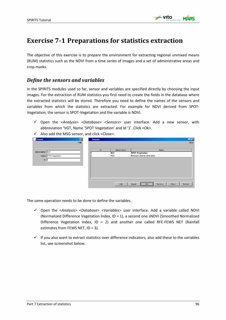
SPIRITS Tutorial


Exercise 7-1 Preparations for statistics extraction

The objective of this exercise is to prepare the environment for extracting regional unmixed means (RUM) statistics such as the NDVI from a time series of images and a set of administrative areas and crop masks.

Define the sensors and variables In the SPIRITS modules used so far, sensor and variables are specified directly by choosing the input images. For the extraction of RUM statistics you first need to create the fields in the database where the extracted statistics will be stored. Therefore you need to define the names of the sensors and variables from which the statistics are extracted. For example for NDVI derived from SPOT-Vegetation, the sensor is SPOT-Vegetation and the variable is NDVI.

Open the <Analysis> <Database> <Sensors> user interface. Add a new sensor, with abbreviation ‘VGT, Name ‘SPOT Vegetation’ and Id ‘1’. Click <Ok>.

Also add the MSG sensor, and click <Close>.

The same operation needs to be done to define the variables.

Open the <Analysis> <Database> <Variables> user interface. Add a variable called NDVI (Normalized Difference Vegetation Index, ID = 1), a second one sNDVI (Smoothed Normalized Difference Vegetation Index, ID = 2) and another one called RFE-FEWS NET (Rainfall estimates from FEWS NET, ID = 3).

If you also want to extract statistics over difference indicators, also add these to the variables list, see screenshot below.

SPIRITS Tutorial


Note that the definition of sensors and variables is specific to each SPIRITS project. If you create a new project (and hence a new database), this information will need to be imported again.

Define the administrative regions The definition of the administrative regions is similar to the sensors and variables. The region names and IDs can be imported from text files or directly from Shapefiles. You will use the same Shapefile as was used in Exercise 4-6 Rasterize Shapefiles for the import of region names and IDs.

Open the <Analysis> <Database> <Regions> user interface. Click <Add> and create a new regions set called SEN_Reg (Senegal Regions, ID=1) and click

<Ok>. Now click on the (just added) regions set item at the top of the dialogue box, and click

<Import> in order to import regions in this regions set. Note that you can import the regions names and IDs from a CSV file, a HDR file, or a SHP file.

You will use the last option: go to the SHP tab, choose \TUTORIAL\DATA\SEN\NDVI\REF\regions.shp as input file. In the bottom part of the ‘Import Regions’ user interface, define which column of the attribute table should be used to define the ID and the Name. Since the attribute table of the Shapefile does not contain region abbreviations (up to 16 characters), add these manually.

Click <Ok> and check the regions settings.

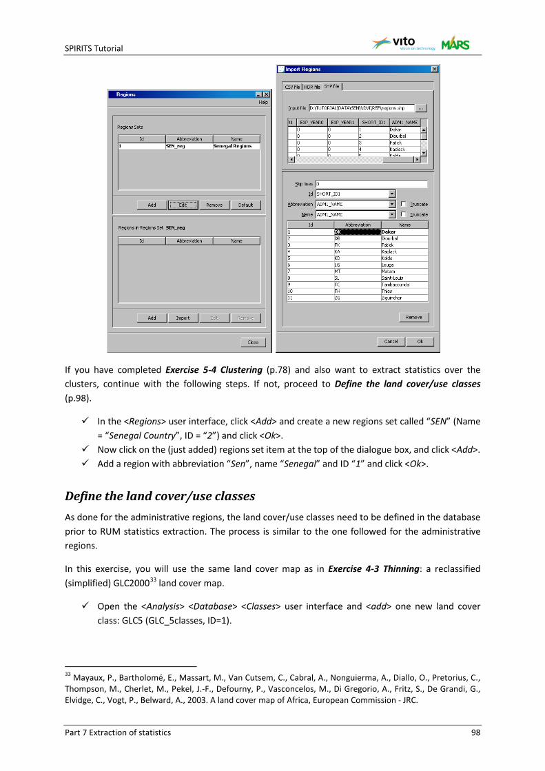
SPIRITS Tutorial


If you have completed Exercise 5-4 Clustering (p.78) and also want to extract statistics over the clusters, continue with the following steps. If not, proceed to Define the land cover/use classes (p.98).

In the <Regions> user interface, click <Add> and create a new regions set called “SEN” (Name = “Senegal Country”, ID = “2”) and click <Ok>.

Now click on the (just added) regions set item at the top of the dialogue box, and click <Add>. Add a region with abbreviation “Sen”, name “Senegal” and ID “1” and click <Ok>.

Define the land cover/use classes As done for the administrative regions, the land cover/use classes need to be defined in the database prior to RUM statistics extraction. The process is similar to the one followed for the administrative regions.

In this exercise, you will use the same land cover map as in Exercise 4-3 Thinning: a reclassified (simplified) GLC200033 land cover map.

Open the <Analysis> <Database> <Classes> user interface and <add> one new land cover class: GLC5 (GLC_5classes, ID=1).

33 Mayaux, P., Bartholomé, E., Massart, M., Van Cutsem, C., Cabral, A., Nonguierma, A., Diallo, O., Pretorius, C., Thompson, M., Cherlet, M., Pekel, J.-F., Defourny, P., Vasconcelos, M., Di Gregorio, A., Fritz, S., De Grandi, G., Elvidge, C., Vogt, P., Belward, A., 2003. A land cover map of Africa, European Commission - JRC.

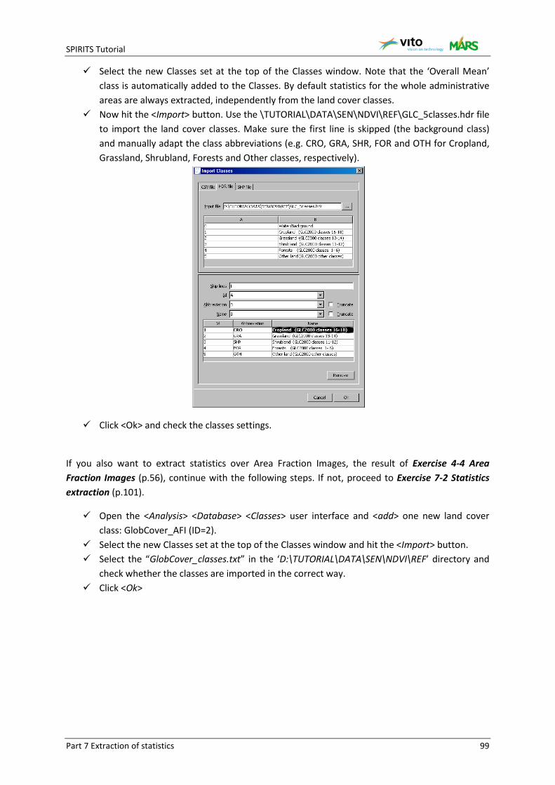
SPIRITS Tutorial


Select the new Classes set at the top of the Classes window. Note that the ‘Overall Mean’ class is automatically added to the Classes. By default statistics for the whole administrative areas are always extracted, independently from the land cover classes.

Now hit the <Import> button. Use the \TUTORIAL\DATA\SEN\NDVI\REF\GLC_5classes.hdr file to import the land cover classes. Make sure the first line is skipped (the background class) and manually adapt the class abbreviations (e.g. CRO, GRA, SHR, FOR and OTH for Cropland, Grassland, Shrubland, Forests and Other classes, respectively).

Click <Ok> and check the classes settings.

If you also want to extract statistics over Area Fraction Images, the result of Exercise 4-4 Area Fraction Images (p.56), continue with the following steps. If not, proceed to Exercise 7-2 Statistics extraction (p.101).

Open the <Analysis> <Database> <Classes> user interface and <add> one new land cover class: GlobCover_AFI (ID=2).

Select the new Classes set at the top of the Classes window and hit the <Import> button. Select the “GlobCover_classes.txt” in the ‘D:\TUTORIAL\DATA\SEN\NDVI\REF’ directory and

check whether the classes are imported in the correct way. Click <Ok>

SPIRITS Tutorial


If you also want to extract statistics over the result of the clustering operations that were performed in Exercise 5-4 Clustering (p.78), continue with the following steps. If not, proceed to Exercise 7-2 Statistics extraction (p.101).

Open the <Analysis> <Database> <Classes> user interface and <add> one new land cover class, with abbreviation “CLU_2012” (Name = “Clustering 2012 NDVI (5 classes)”, ID = “3”).

Select the new Classes set at the top of the Classes window and hit the <Import> button. In the <HDR file> tab, Select the “ongoing_2012_ke.hdr” in the

‘D:\TUTORIAL\DATA\SEN\NDVI\ISO\ACT\S10s’ directory and check whether the classes are imported in the correct way. Remove the ‘Not classified’ class.

Click <Ok>

All elements needed for extracting statistics from image time series for land cover classes within administrative regions have now been set and it is possible to proceed with the actual extraction in Exercise 7-2 Statistics extraction followed by the statistics visualization in Exercise 7-3 Visualization of statistics.

SPIRITS Tutorial


Exercise 7-2 Statistics extraction

The objective of this exercise is to extract RUM statistics for a time series of NDVI and RFE over administrative regions in Senegal by using land cover masks derived from the (simplified) GLC2000 dataset. The statistics will then be visualized as seasonal vegetation monitoring graphs.

This exercise builds on the preparations done in the previous Exercise 7-1 Preparations for statistics extraction and cannot be started until the preparatory steps were completed successfully.

RUM extraction scenario for extracting NDVI Open the <Analysis> <Database> <Extract> <Time series> user interface and create a new

scenario. Define the scenario name as “SEN_RUMExtract_NDVI_ACT_S10s_regions_GLC5”: you will

extract statistics over 10-daily smoothed NDVI time series over the regions of Senegal and 5 generalized GLC classes.

Define the periodicity (dekad), the input directory (‘D:\TUTORIAL\DATA\SEN\NDVI\ACT\S10s’) and naming format (vtYYYYMMDDk) of the input images.

As output directory, choose ‘D:\TUTORIAL\RUM\SEN\regions_GLC5’ and keep the same naming structure for the output RUM files.

Define the sensor (VGT) and variable (sNDVI) and leave the ‘include explanations’ box unchecked34.

Click on <New> in order to create a new SPU (RUM Specification) file: this is an additional information file needed for RUM extraction and specifies which reference raster images (regions, classes) will be used for the statistics calculation.

In the ‘SPU Unmixing Specification’ window enter the name of the regions file: “D:\TUTORIAL\DATA\SEN\NDVI\REF\regions.img”. Leave the optional ‘region Id’s subset’ field empty.

! The ‘Region Id’s subset’ field is only needed in case statistics should be extracted only for a subset of the regions included in the administrative regions image. A comma-separated ascii file can be used as input (see also the SPIRITS Manual). If it is left empty statistics will be extracted for all the regions.

Note that there are three options in the Land Use/Cover part of the window: ‘No Land Use classification’, ‘Hard classification’ and ‘Area Fractions’. In this case you will use a ‘Hard classification’: each pixel corresponds to one land cover class. Select ‘GLC5’ as the classes set to import the classes from. Click <Import> and see how the classes appear. Now select ‘D:\TUTORIAL\DATA\SEN\NDVI\REF\GLC_5classes.img’ as the raster image to use for statistics extraction.

34 This option will include explanations in the output RUM files, which can be useful when the RUM files are used for processing in other software than SPIRITS.

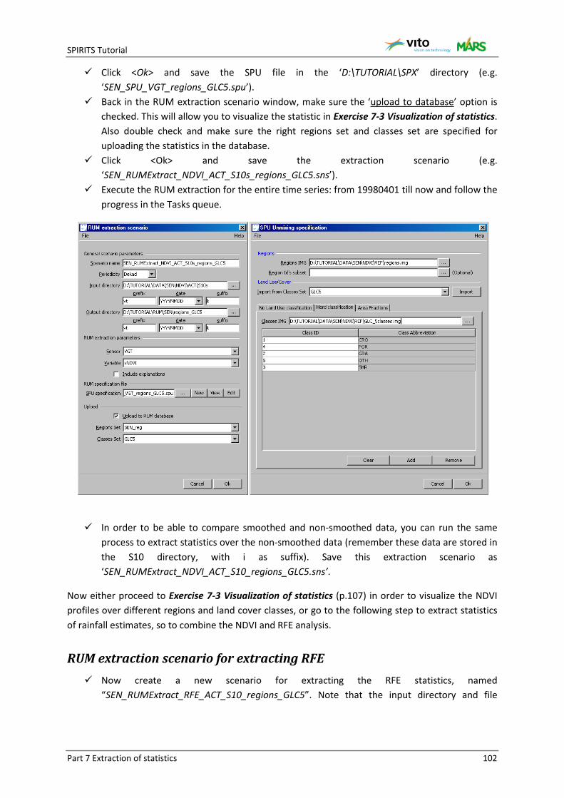
SPIRITS Tutorial


Click <Ok> and save the SPU file in the ‘D:\TUTORIAL\SPX’ directory (e.g. ‘SEN_SPU_VGT_regions_GLC5.spu’).

Back in the RUM extraction scenario window, make sure the ‘upload to database’ option is checked. This will allow you to visualize the statistic in Exercise 7-3 Visualization of statistics. Also double check and make sure the right regions set and classes set are specified for uploading the statistics in the database.

Click <Ok> and save the extraction scenario (e.g. ‘SEN_RUMExtract_NDVI_ACT_S10s_regions_GLC5.sns’).

Execute the RUM extraction for the entire time series: from 19980401 till now and follow the progress in the Tasks queue.

In order to be able to compare smoothed and non-smoothed data, you can run the same

process to extract statistics over the non-smoothed data (remember these data are stored in the S10 directory, with i as suffix). Save this extraction scenario as ‘SEN_RUMExtract_NDVI_ACT_S10_regions_GLC5.sns’.

Now either proceed to Exercise 7-3 Visualization of statistics (p.107) in order to visualize the NDVI profiles over different regions and land cover classes, or go to the following step to extract statistics of rainfall estimates, so to combine the NDVI and RFE analysis.

RUM extraction scenario for extracting RFE Now create a new scenario for extracting the RFE statistics, named

“SEN_RUMExtract_RFE_ACT_S10_regions_GLC5”. Note that the input directory and file

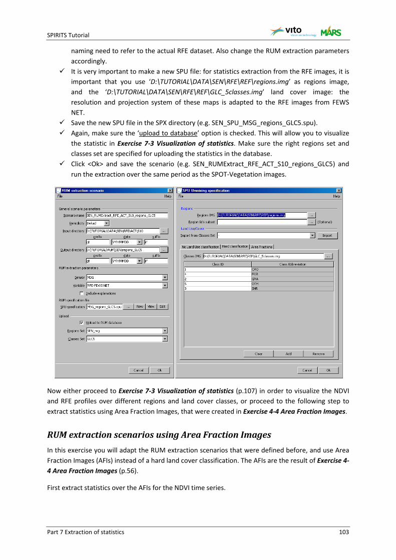
SPIRITS Tutorial


naming need to refer to the actual RFE dataset. Also change the RUM extraction parameters accordingly.

It is very important to make a new SPU file: for statistics extraction from the RFE images, it is important that you use ‘D:\TUTORIAL\DATA\SEN\RFE\REF\regions.img’ as regions image, and the ‘D:\TUTORIAL\DATA\SEN\RFE\REF\GLC_5classes.img’ land cover image: the resolution and projection system of these maps is adapted to the RFE images from FEWS NET.

Save the new SPU file in the SPX directory (e.g. SEN_SPU_MSG_regions_GLC5.spu). Again, make sure the ‘upload to database’ option is checked. This will allow you to visualize

the statistic in Exercise 7-3 Visualization of statistics. Make sure the right regions set and classes set are specified for uploading the statistics in the database.

Click <Ok> and save the scenario (e.g. SEN_RUMExtract_RFE_ACT_S10_regions_GLC5) and run the extraction over the same period as the SPOT-Vegetation images.

Now either proceed to Exercise 7-3 Visualization of statistics (p.107) in order to visualize the NDVI and RFE profiles over different regions and land cover classes, or proceed to the following step to extract statistics using Area Fraction Images, that were created in Exercise 4-4 Area Fraction Images.

RUM extraction scenarios using Area Fraction Images In this exercise you will adapt the RUM extraction scenarios that were defined before, and use Area Fraction Images (AFIs) instead of a hard land cover classification. The AFIs are the result of Exercise 4-4 Area Fraction Images (p.56).

First extract statistics over the AFIs for the NDVI time series.

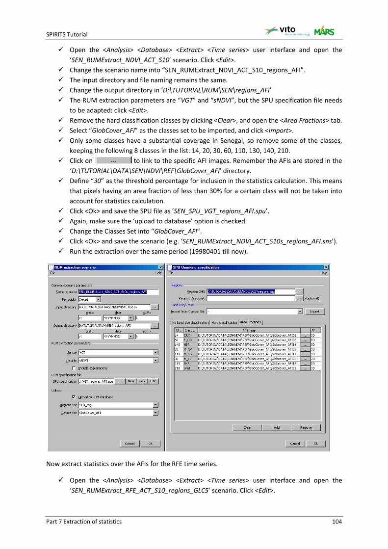
SPIRITS Tutorial


Open the <Analysis> <Database> <Extract> <Time series> user interface and open the ‘SEN_RUMExtract_NDVI_ACT_S10’ scenario. Click <Edit>.

Change the scenario name into “SEN_RUMExtract_NDVI_ACT_S10_regions_AFI”. The input directory and file naming remains the same. Change the output directory in ‘D:\TUTORIAL\RUM\SEN\regions_AFI’ The RUM extraction parameters are “VGT” and “sNDVI”, but the SPU specification file needs

to be adapted: click <Edit>. Remove the hard classification classes by clicking <Clear>, and open the <Area Fractions> tab. Select “GlobCover_AFI” as the classes set to be imported, and click <Import>. Only some classes have a substantial coverage in Senegal, so remove some of the classes,

keeping the following 8 classes in the list: 14, 20, 30, 60, 110, 130, 140, 210. Click on to link to the specific AFI images. Remember the AFIs are stored in the

‘D:\TUTORIAL\DATA\SEN\NDVI\REF\GlobCover_AFI’ directory. Define “30” as the threshold percentage for inclusion in the statistics calculation. This means

that pixels having an area fraction of less than 30% for a certain class will not be taken into account for statistics calculation.

Click <Ok> and save the SPU file as ‘SEN_SPU_VGT_regions_AFI.spu’. Again, make sure the ‘upload to database’ option is checked. Change the Classes Set into “GlobCover_AFI”. Click <Ok> and save the scenario (e.g. ‘SEN_RUMExtract_NDVI_ACT_S10s_regions_AFI.sns’). Run the extraction over the same period (19980401 till now).

Now extract statistics over the AFIs for the RFE time series.

Open the <Analysis> <Database> <Extract> <Time series> user interface and open the ‘SEN_RUMExtract_RFE_ACT_S10_regions_GLC5’ scenario. Click <Edit>.

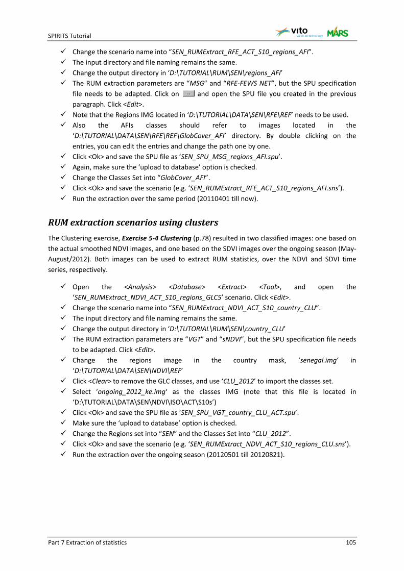
SPIRITS Tutorial


Change the scenario name into “SEN_RUMExtract_RFE_ACT_S10_regions_AFI”. The input directory and file naming remains the same. Change the output directory in ‘D:\TUTORIAL\RUM\SEN\regions_AFI’ The RUM extraction parameters are “MSG” and “RFE-FEWS NET”, but the SPU specification

file needs to be adapted. Click on and open the SPU file you created in the previous paragraph. Click <Edit>.

Note that the Regions IMG located in ‘D:\TUTORIAL\DATA\SEN\RFE\REF’ needs to be used. Also the AFIs classes should refer to images located in the

‘D:\TUTORIAL\DATA\SEN\RFE\REF\GlobCover_AFI’ directory. By double clicking on the entries, you can edit the entries and change the path one by one.

Click <Ok> and save the SPU file as ‘SEN_SPU_MSG_regions_AFI.spu’. Again, make sure the ‘upload to database’ option is checked. Change the Classes Set into “GlobCover_AFI”. Click <Ok> and save the scenario (e.g. ‘SEN_RUMExtract_RFE_ACT_S10_regions_AFI.sns’). Run the extraction over the same period (20110401 till now).

RUM extraction scenarios using clusters The Clustering exercise, Exercise 5-4 Clustering (p.78) resulted in two classified images: one based on the actual smoothed NDVI images, and one based on the SDVI images over the ongoing season (May-August/2012). Both images can be used to extract RUM statistics, over the NDVI and SDVI time series, respectively.

Open the <Analysis> <Database> <Extract> <Tool>, and open the ‘SEN_RUMExtract_NDVI_ACT_S10_regions_GLC5’ scenario. Click <Edit>.

Change the scenario name into “SEN_RUMExtract_NDVI_ACT_S10_country_CLU”. The input directory and file naming remains the same. Change the output directory in ‘D:\TUTORIAL\RUM\SEN\country_CLU’ The RUM extraction parameters are “VGT” and “sNDVI”, but the SPU specification file needs

to be adapted. Click <Edit>. Change the regions image in the country mask, ‘senegal.img‘ in

‘D:\TUTORIAL\DATA\SEN\NDVI\REF’ Click <Clear> to remove the GLC classes, and use ‘CLU_2012’ to import the classes set. Select ‘ongoing_2012_ke.img‘ as the classes IMG (note that this file is located in

‘D:\TUTORIAL\DATA\SEN\NDVI\ISO\ACT\S10s’) Click <Ok> and save the SPU file as ‘SEN_SPU_VGT_country_CLU_ACT.spu’. Make sure the ‘upload to database’ option is checked. Change the Regions set into “SEN” and the Classes Set into “CLU_2012”. Click <Ok> and save the scenario (e.g. ‘SEN_RUMExtract_NDVI_ACT_S10_regions_CLU.sns’). Run the extraction over the ongoing season (20120501 till 20120821).

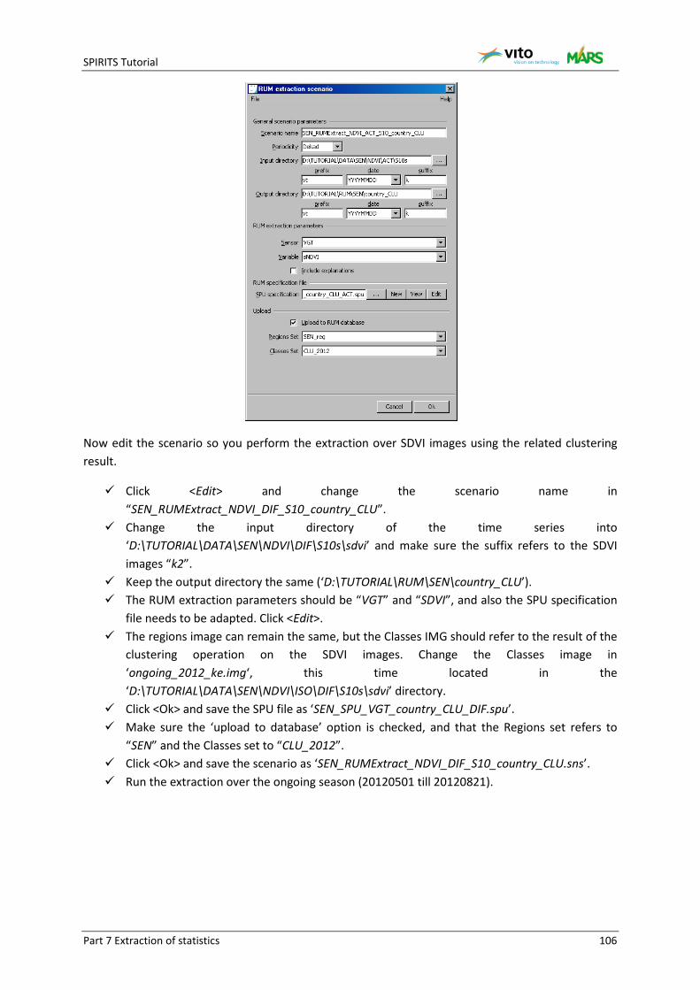
SPIRITS Tutorial


Now edit the scenario so you perform the extraction over SDVI images using the related clustering result.

Click <Edit> and change the scenario name in “SEN_RUMExtract_NDVI_DIF_S10_country_CLU”.

Change the input directory of the time series into ‘D:\TUTORIAL\DATA\SEN\NDVI\DIF\S10s\sdvi’ and make sure the suffix refers to the SDVI images “k2”.

Keep the output directory the same (‘D:\TUTORIAL\RUM\SEN\country_CLU’). The RUM extraction parameters should be “VGT” and “SDVI”, and also the SPU specification

file needs to be adapted. Click <Edit>. The regions image can remain the same, but the Classes IMG should refer to the result of the

clustering operation on the SDVI images. Change the Classes image in ‘ongoing_2012_ke.img‘, this time located in the ‘D:\TUTORIAL\DATA\SEN\NDVI\ISO\DIF\S10s\sdvi’ directory.

Click <Ok> and save the SPU file as ‘SEN_SPU_VGT_country_CLU_DIF.spu’. Make sure the ‘upload to database’ option is checked, and that the Regions set refers to

“SEN” and the Classes set to “CLU_2012”. Click <Ok> and save the scenario as ‘SEN_RUMExtract_NDVI_DIF_S10_country_CLU.sns’. Run the extraction over the ongoing season (20120501 till 20120821).

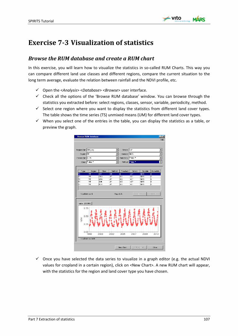
SPIRITS Tutorial


Exercise 7-3 Visualization of statistics

Browse the RUM database and create a RUM chart In this exercise, you will learn how to visualize the statistics in so-called RUM Charts. This way you can compare different land use classes and different regions, compare the current situation to the long term average, evaluate the relation between rainfall and the NDVI profile, etc.

Open the <Analysis> <Database> <Browse> user interface. Check all the options of the ‘Browse RUM database’ window. You can browse through the

statistics you extracted before: select regions, classes, sensor, variable, periodicity, method. Select one region where you want to display the statistics from different land cover types.

The table shows the time series (TS) unmixed means (UM) for different land cover types. When you select one of the entries in the table, you can display the statistics as a table, or

preview the graph.

Once you have selected the data series to visualize in a graph editor (e.g. the actual NDVI values for cropland in a certain region), click on <New Chart>. A new RUM chart will appear, with the statistics for the region and land cover type you have chosen.

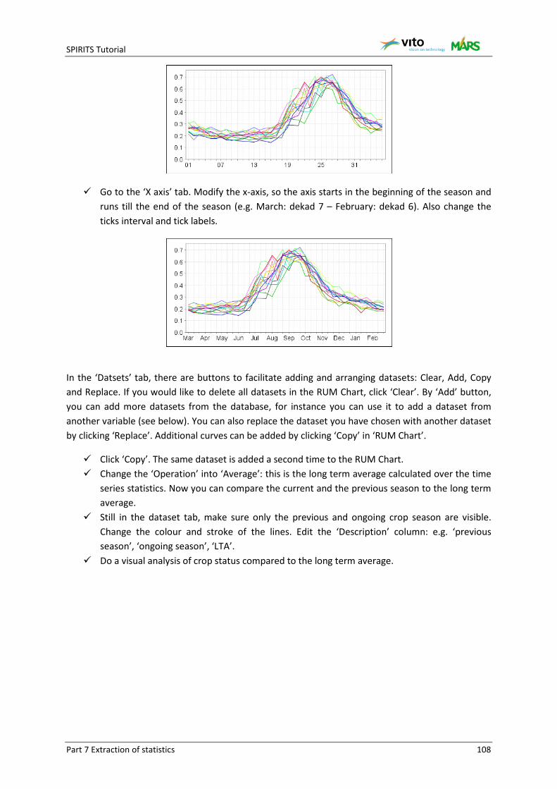
SPIRITS Tutorial


Go to the ‘X axis’ tab. Modify the x-axis, so the axis starts in the beginning of the season and runs till the end of the season (e.g. March: dekad 7 – February: dekad 6). Also change the ticks interval and tick labels.

In the ‘Datsets’ tab, there are buttons to facilitate adding and arranging datasets: Clear, Add, Copy and Replace. If you would like to delete all datasets in the RUM Chart, click ‘Clear’. By ‘Add’ button, you can add more datasets from the database, for instance you can use it to add a dataset from another variable (see below). You can also replace the dataset you have chosen with another dataset by clicking ‘Replace’. Additional curves can be added by clicking ‘Copy’ in ‘RUM Chart’.

Click ‘Copy’. The same dataset is added a second time to the RUM Chart. Change the ‘Operation’ into ‘Average’: this is the long term average calculated over the time

series statistics. Now you can compare the current and the previous season to the long term average.

Still in the dataset tab, make sure only the previous and ongoing crop season are visible. Change the colour and stroke of the lines. Edit the ‘Description’ column: e.g. ‘previous season’, ‘ongoing season’, ‘LTA’.

Do a visual analysis of crop status compared to the long term average.

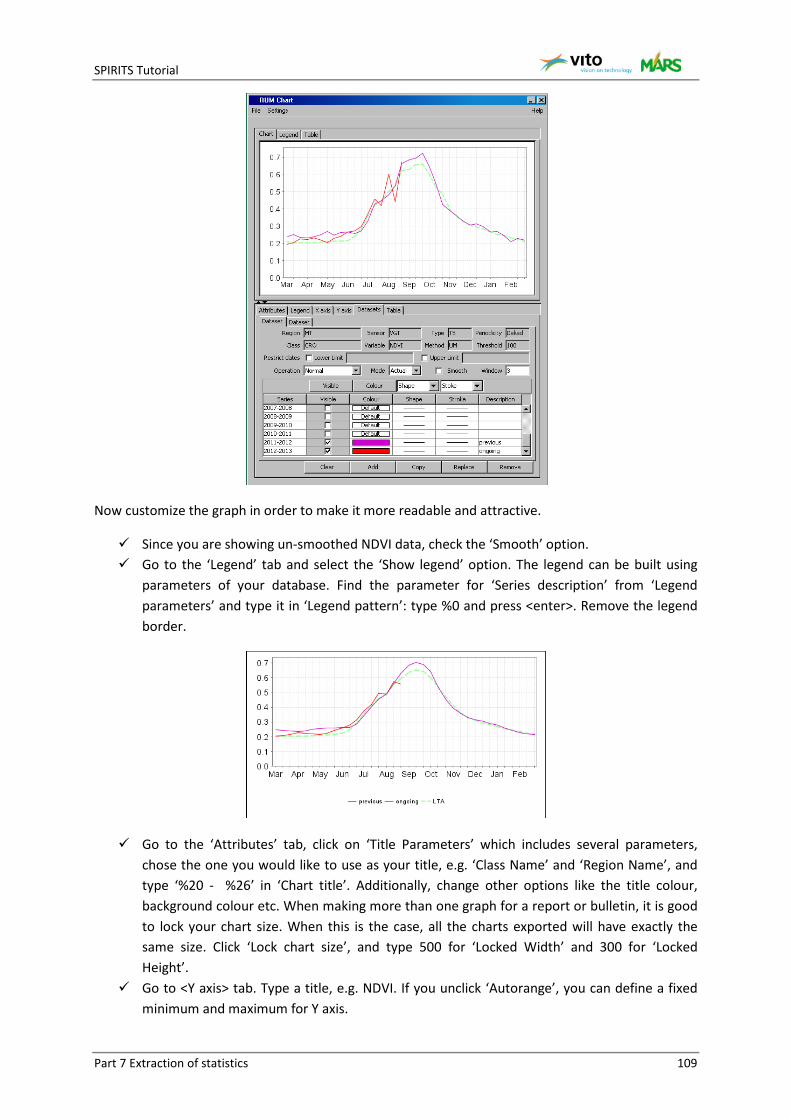
SPIRITS Tutorial


Now customize the graph in order to make it more readable and attractive.

Since you are showing un-smoothed NDVI data, check the ‘Smooth’ option. Go to the ‘Legend’ tab and select the ‘Show legend’ option. The legend can be built using

parameters of your database. Find the parameter for ‘Series description’ from ‘Legend parameters’ and type it in ‘Legend pattern’: type %0 and press <enter>. Remove the legend border.

Go to the ‘Attributes’ tab, click on ‘Title Parameters’ which includes several parameters, chose the one you would like to use as your title, e.g. ‘Class Name’ and ‘Region Name’, and type ‘%20 - %26’ in ‘Chart title’. Additionally, change other options like the title colour, background colour etc. When making more than one graph for a report or bulletin, it is good to lock your chart size. When this is the case, all the charts exported will have exactly the same size. Click ‘Lock chart size’, and type 500 for ‘Locked Width’ and 300 for ‘Locked Height’.

Go to <Y axis> tab. Type a title, e.g. NDVI. If you unclick ‘Autorange’, you can define a fixed minimum and maximum for Y axis.

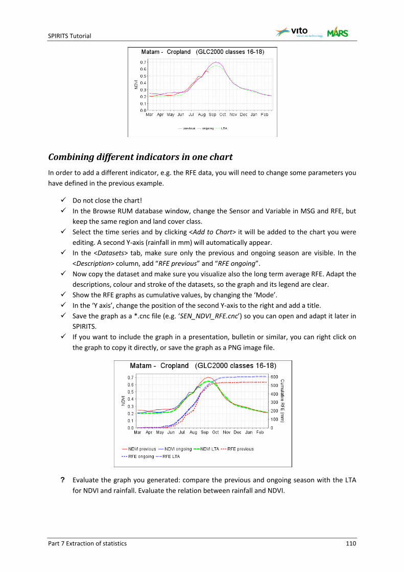
SPIRITS Tutorial


Combining different indicators in one chart In order to add a different indicator, e.g. the RFE data, you will need to change some parameters you have defined in the previous example.

Do not close the chart! In the Browse RUM database window, change the Sensor and Variable in MSG and RFE, but

keep the same region and land cover class. Select the time series and by clicking <Add to Chart> it will be added to the chart you were

editing. A second Y-axis (rainfall in mm) will automatically appear. In the <Datasets> tab, make sure only the previous and ongoing season are visible. In the

<Description> column, add “RFE previous” and “RFE ongoing”. Now copy the dataset and make sure you visualize also the long term average RFE. Adapt the

descriptions, colour and stroke of the datasets, so the graph and its legend are clear. Show the RFE graphs as cumulative values, by changing the ‘Mode’. In the ‘Y axis’, change the position of the second Y-axis to the right and add a title. Save the graph as a *.cnc file (e.g. ‘SEN_NDVI_RFE.cnc’) so you can open and adapt it later in

SPIRITS. If you want to include the graph in a presentation, bulletin or similar, you can right click on

the graph to copy it directly, or save the graph as a PNG image file.

? Evaluate the graph you generated: compare the previous and ongoing season with the LTA for NDVI and rainfall. Evaluate the relation between rainfall and NDVI.

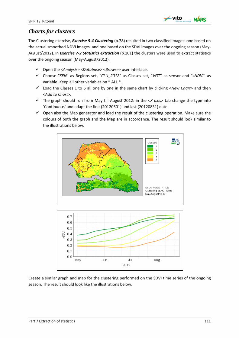
SPIRITS Tutorial


Charts for clusters The Clustering exercise, Exercise 5-4 Clustering (p.78) resulted in two classified images: one based on the actual smoothed NDVI images, and one based on the SDVI images over the ongoing season (May-August/2012). In Exercise 7-2 Statistics extraction (p.101) the clusters were used to extract statistics over the ongoing season (May-August/2012).

Open the <Analysis> <Database> <Browse> user interface. Choose “SEN” as Regions set, “CLU_2012” as Classes set, “VGT” as sensor and “sNDVI” as

variable. Keep all other variables on * ALL *. Load the Classes 1 to 5 all one by one in the same chart by clicking <New Chart> and then

<Add to Chart>. The graph should run from May till August 2012: in the <X axis> tab change the type into

‘Continuous’ and adapt the first (20120501) and last (20120831) date. Open also the Map generator and load the result of the clustering operation. Make sure the

colours of both the graph and the Map are in accordance. The result should look similar to the illustrations below.

Create a similar graph and map for the clustering performed on the SDVI time series of the ongoing season. The result should look like the illustrations below.

SPIRITS Tutorial


? Which areas show a vegetation status above normal throughout the ongoing season? Which not? Can you relate this to rainfall anomalies (positive or negative)?

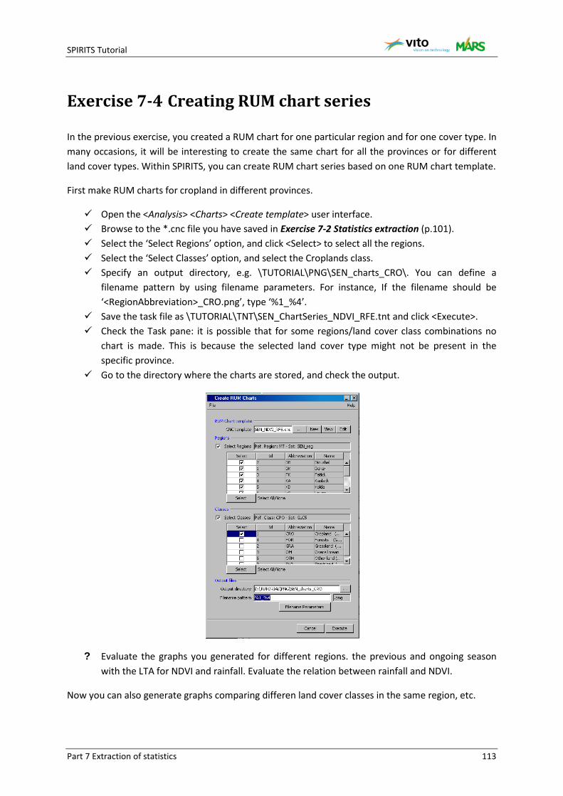
SPIRITS Tutorial


Exercise 7-4 Creating RUM chart series

In the previous exercise, you created a RUM chart for one particular region and for one cover type. In many occasions, it will be interesting to create the same chart for all the provinces or for different land cover types. Within SPIRITS, you can create RUM chart series based on one RUM chart template.

First make RUM charts for cropland in different provinces.

Open the <Analysis> <Charts> <Create template> user interface. Browse to the *.cnc file you have saved in Exercise 7-2 Statistics extraction (p.101). Select the ‘Select Regions’ option, and click <Select> to select all the regions. Select the ‘Select Classes’ option, and select the Croplands class. Specify an output directory, e.g. \TUTORIAL\PNG\SEN_charts_CRO\. You can define a

filename pattern by using filename parameters. For instance, If the filename should be ‘<RegionAbbreviation>_CRO.png’, type ‘%1_%4’.

Save the task file as \TUTORIAL\TNT\SEN_ChartSeries_NDVI_RFE.tnt and click <Execute>. Check the Task pane: it is possible that for some regions/land cover class combinations no

chart is made. This is because the selected land cover type might not be present in the specific province.

Go to the directory where the charts are stored, and check the output.

? Evaluate the graphs you generated for different regions. the previous and ongoing season with the LTA for NDVI and rainfall. Evaluate the relation between rainfall and NDVI.

Now you can also generate graphs comparing differen land cover classes in the same region, etc.

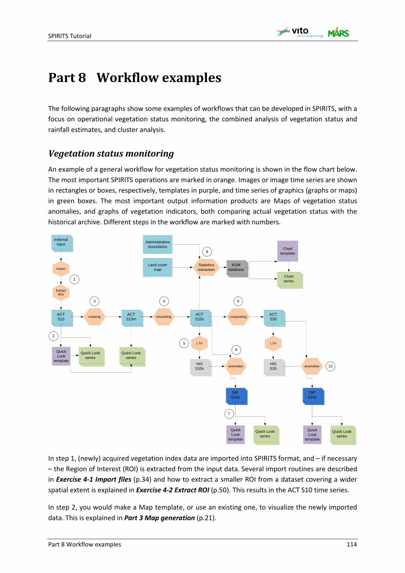
SPIRITS Tutorial

Part 8 Workflow examples 114

Part 8 Workflow examples

The following paragraphs show some examples of workflows that can be developed in SPIRITS, with a focus on operational vegetation status monitoring, the combined analysis of vegetation status and rainfall estimates, and cluster analysis.

Vegetation status monitoring An example of a general workflow for vegetation status monitoring is shown in the flow chart below. The most important SPIRITS operations are marked in orange. Images or image time series are shown in rectangles or boxes, respectively, templates in purple, and time series of graphics (graphs or maps) in green boxes. The most important output information products are Maps of vegetation status anomalies, and graphs of vegetation indicators, both comparing actual vegetation status with the historical archive. Different steps in the workflow are marked with numbers.

ACTS10

Extract ROI

ACTS10m

ACTS10smasking smoothing

Import

ACTS30compositing

LTA LTA

HISS10s

HISS30anomalies anomalies

DIFS10s

Quick Look

template

Quick Look series

Statistics extraction

Administrative boundaries

Land cover map

Charttemplate

Chart series1

2

3

Quick Look series

4

56

Quick Look

template

Quick Look series

7

DIFS10s

Quick Look

template

Quick Look series

9

8

RUM database

10

external input

In step 1, (newly) acquired vegetation index data are imported into SPIRITS format, and – if necessary – the Region of Interest (ROI) is extracted from the input data. Several import routines are described in Exercise 4-1 Import files (p.34) and how to extract a smaller ROI from a dataset covering a wider spatial extent is explained in Exercise 4-2 Extract ROI (p.50). This results in the ACT S10 time series.

In step 2, you would make a Map template, or use an existing one, to visualize the newly imported data. This is explained in Part 3 Map generation (p.21).

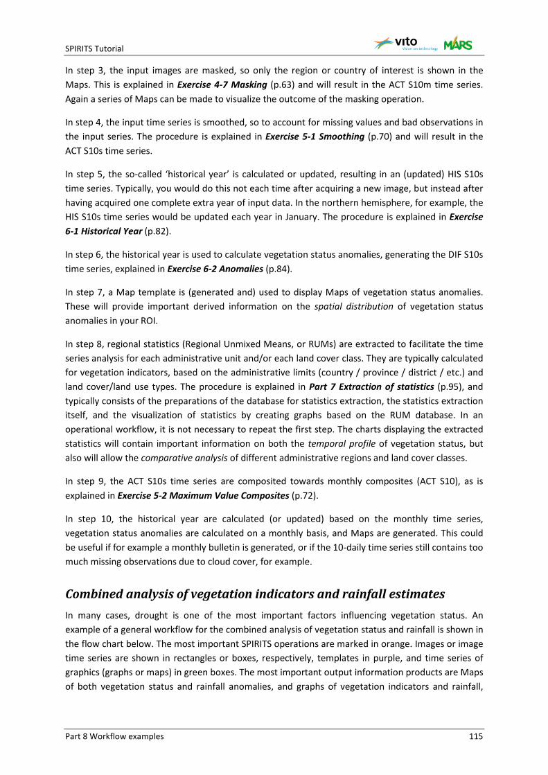
SPIRITS Tutorial


In step 3, the input images are masked, so only the region or country of interest is shown in the Maps. This is explained in Exercise 4-7 Masking (p.63) and will result in the ACT S10m time series. Again a series of Maps can be made to visualize the outcome of the masking operation.

In step 4, the input time series is smoothed, so to account for missing values and bad observations in the input series. The procedure is explained in Exercise 5-1 Smoothing (p.70) and will result in the ACT S10s time series.

In step 5, the so-called ‘historical year’ is calculated or updated, resulting in an (updated) HIS S10s time series. Typically, you would do this not each time after acquiring a new image, but instead after having acquired one complete extra year of input data. In the northern hemisphere, for example, the HIS S10s time series would be updated each year in January. The procedure is explained in Exercise 6-1 Historical Year (p.82).

In step 6, the historical year is used to calculate vegetation status anomalies, generating the DIF S10s time series, explained in Exercise 6-2 Anomalies (p.84).

In step 7, a Map template is (generated and) used to display Maps of vegetation status anomalies. These will provide important derived information on the spatial distribution of vegetation status anomalies in your ROI.

In step 8, regional statistics (Regional Unmixed Means, or RUMs) are extracted to facilitate the time series analysis for each administrative unit and/or each land cover class. They are typically calculated for vegetation indicators, based on the administrative limits (country / province / district / etc.) and land cover/land use types. The procedure is explained in Part 7 Extraction of statistics (p.95), and typically consists of the preparations of the database for statistics extraction, the statistics extraction itself, and the visualization of statistics by creating graphs based on the RUM database. In an operational workflow, it is not necessary to repeat the first step. The charts displaying the extracted statistics will contain important information on both the temporal profile of vegetation status, but also will allow the comparative analysis of different administrative regions and land cover classes.

In step 9, the ACT S10s time series are composited towards monthly composites (ACT S10), as is explained in Exercise 5-2 Maximum Value Composites (p.72).

In step 10, the historical year are calculated (or updated) based on the monthly time series, vegetation status anomalies are calculated on a monthly basis, and Maps are generated. This could be useful if for example a monthly bulletin is generated, or if the 10-daily time series still contains too much missing observations due to cloud cover, for example.

Combined analysis of vegetation indicators and rainfall estimates In many cases, drought is one of the most important factors influencing vegetation status. An example of a general workflow for the combined analysis of vegetation status and rainfall is shown in the flow chart below. The most important SPIRITS operations are marked in orange. Images or image time series are shown in rectangles or boxes, respectively, templates in purple, and time series of graphics (graphs or maps) in green boxes. The most important output information products are Maps of both vegetation status and rainfall anomalies, and graphs of vegetation indicators and rainfall,

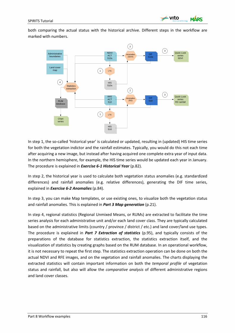
SPIRITS Tutorial


both comparing the actual status with the historical archive. Different steps in the workflow are marked with numbers.

NDVI ACTS10s

LTA

HISS10s

Anomalies (SDVI)

DIFS10s

4

Quick Look seriesSDVI

RFE ACTS10

LTA

HISS10

Anomalies (RD)

DIFS10

Quick Look series

RD rainfall


Administrative boundaries

Land cover map

Chart series

1

RUM database

1

2

2

3

3

In step 1, the so-called ‘historical year’ is calculated or updated, resulting in (updated) HIS time series for both the vegetation indictor and the rainfall estimates. Typically, you would do this not each time after acquiring a new image, but instead after having acquired one complete extra year of input data. In the northern hemisphere, for example, the HIS time series would be updated each year in January. The procedure is explained in Exercise 6-1 Historical Year (p.82).

In step 2, the historical year is used to calculate both vegetation status anomalies (e.g. standardized differences) and rainfall anomalies (e.g. relative differences), generating the DIF time series, explained in Exercise 6-2 Anomalies (p.84).

In step 3, you can make Map templates, or use existing ones, to visualize both the vegetation status and rainfall anomalies. This is explained in Part 3 Map generation (p.21).

In step 4, regional statistics (Regional Unmixed Means, or RUMs) are extracted to facilitate the time series analysis for each administrative unit and/or each land cover class. They are typically calculated based on the administrative limits (country / province / district / etc.) and land cover/land use types. The procedure is explained in Part 7 Extraction of statistics (p.95), and typically consists of the preparations of the database for statistics extraction, the statistics extraction itself, and the visualization of statistics by creating graphs based on the RUM database. In an operational workflow, it is not necessary to repeat the first step. The statistics extraction operation can be done on both the actual NDVI and RFE images, and on the vegetation and rainfall anomalies. The charts displaying the extracted statistics will contain important information on both the temporal profile of vegetation status and rainfall, but also will allow the comparative analysis of different administrative regions and land cover classes.

SPIRITS Tutorial


Cluster analysis Cluster analysis is an interesting tool to create unsupervised classifications based on a time series of e.g. vegetation indicators or vegetation anomalies, whereby an ISODATA method is used to cluster the pixels according to their similar time profile.

An example of a general workflow for the cluster analysis of vegetation status and vegetation anomalies is shown in the flow chart below. The most important SPIRITS operations are marked in orange. Images or image time series are shown in rectangles or boxes, respectively, templates in purple, and time series of graphics (graphs or maps) in green boxes. The most important output information products are Maps of clusters of both vegetation status and vegetation anomalies, and graphs of vegetation indicators and vegetation anomalies over the respective clusters. Different steps in the workflow are marked with numbers.


RUM database

Mask image

NDVI ACTS10s

SDVI DIF

S10s

ISO Clustering Clusters

ClustersISO Clustering

Cluster RUM Charts

Cluster Quick Look

Cluster Quick Look

1 2

3

1 2

In step 1, the ISO Clustering tool of SPIRITS is used to perform an unsupervised classification over both the actual NDVI time series of the ongoing season, and the vegetation anomalies (SDVI) over the same period. As input, also a mask image is used, which can be e.g. the entire country, or a crop mask in order to perform the analysis only on rainfed crops. The result of the clustering operations are two classification images. The Clustering tool is described in Exercise 5-4 Clustering (p.78).

In step 2, the cluster classification images are visualized in Maps. This is explained in Part 3 Map generation (p.21).

In step 3, both the mask image used for clustering, and the output cluster classification images are used as the ‘regions’ and ‘classes’ layers to extract statistics over the actual vegetation status and vegetation anomalies, respectively. The procedure is explained in Part 7 Extraction of statistics (p.95), and typically consists of the preparations of the database for statistics extraction, the statistics extraction itself, and the visualization of statistics by creating graphs based on the RUM database. The charts displaying the extracted statistics for the clusters should be prepared in accordance with the colour coding used for the Cluster Maps. See also Exercise 7-3 Visualization of statistics (p.107).

tutorial - africa - vito

Documents