tutorial 4. simulation of flow development in a...

Tutorial 4. Simulation of Flow Development in a Pipe

Introduction

The purpose of this tutorial is to illustrate the setup and solution of a 3D turbulentfluid flow in a pipe. The pipe networks are common in any engineering industry. It isimportant to know the development of a flow at the pipe entrance and pressure droptaking place along the pipe length. The flow of fluids in a pipe is widely studied fluidmechanics problem. The correlations for entry length and pressure drop are available interms of flow Reynolds number.

In this tutorial you will learn how to:

• Read an existing mesh file in FLUENT.

• Verify the grid for dimensions and quality.

• Add a new material from materials database.

• Define solver settings and perform iterations.

• Examine the results and compare them with experimental data.

• Visualize the flow field using animation tool.

• Control the view by reading in a file.

Prerequisites

This tutorial assumes that you have little experience with FLUENT but are familiar withthe interface.

Problem Description

Consider a pipe of diameter 1 m and a length of 20 m (Figure 4.1). The geometry issymmetric therefore you will model only half portion of the pipe. Water enters from theinlet boundary with a velocity of 0.015 m/sec. The flow Reynolds number is 15000.

c© Fluent Inc. August 18, 2005 4-1

Simulation of Flow Development in a Pipe

Figure 4.1: Problem Schematic

Preparation

1. Copy the mesh file, pipe.msh and the view file, view-file to your working direc-tory.

2. Start the 3D double precision solver of FLUENT.

Setup and Solution

Step 1: Grid

1. Read the grid file, pipe.msh.

File −→ Read −→Case...

FLUENT will read the mesh file and report the progress in the console window.

2. Check the grid.

Grid −→Check

This procedure checks the integrity of the mesh. Make sure the reported minimumvolume is a positive number.

3. Check the scale of the grid.

Grid −→Scale...

4-2 c© Fluent Inc. August 18, 2005


Check the domain extents to see if they correspond to the actual physical dimensions.If not, the grid has to be scaled with proper units.

4. Display the grid (Figure 4.2).

Display −→Grid...

(a) Click Colors....

The Grid Colors panel opens.



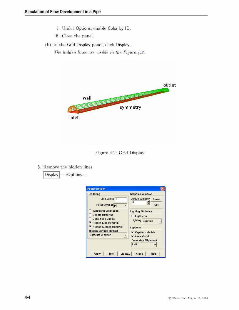
i. Under Options, enable Color by ID.

ii. Close the panel.

(b) In the Grid Display panel, click Display.

The hidden lines are visible in the Figure 4.2.

Figure 4.2: Grid Display

5. Remove the hidden lines.

Display −→Options...



(a) Enable Hidden Line Removal.

(b) Select Software Z-buffer in the Hidden Surface Method drop-down list.

(c) Click Apply and close the panel.

The graphics window will get updated.

(d) Zoom-in the graphics window to get the display as shown in Figure 4.3.

Figure 4.3: Grid Display—Zoomed-in View

Step 2: Models

1. Keep the default solver settings.

Define −→ Models −→Solver...

The problem is solved in steady state using segregated solver, therefore, keep thedefault solver settings.

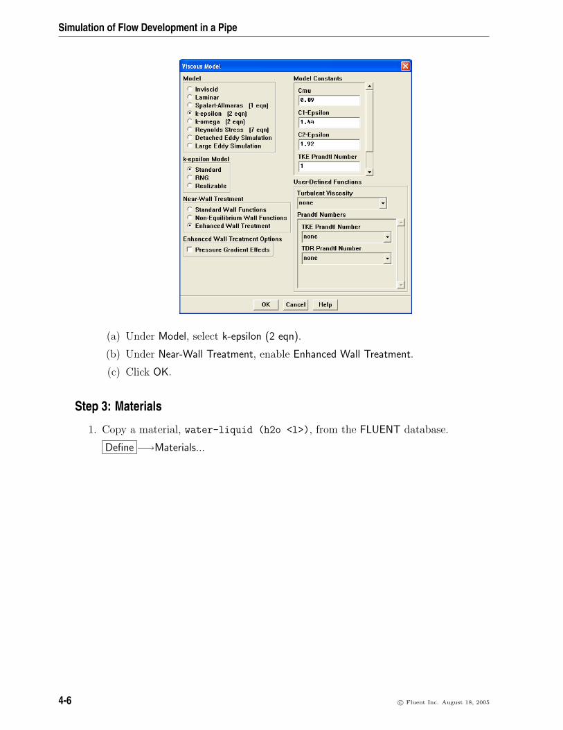
2. Enable the standard k − ε turbulence model.

Solve −→ Models −→Viscous...



(a) Under Model, select k-epsilon (2 eqn).

(b) Under Near-Wall Treatment, enable Enhanced Wall Treatment.

(c) Click OK.

Step 3: Materials

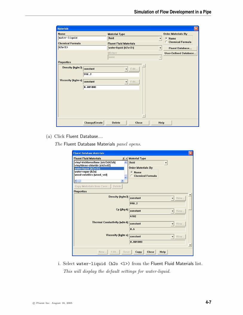
1. Copy a material, water-liquid (h2o <l>), from the FLUENT database.

Define −→Materials...



(a) Click Fluent Database....

The Fluent Database Materials panel opens.

i. Select water-liquid (h2o <l>) from the Fluent Fluid Materials list.

This will display the default settings for water-liquid.



ii. Click Copy and close the panel.

The Materials panel will now display the copied information of water.

(b) Close Materials the panel.

Step 4: Boundary Conditions

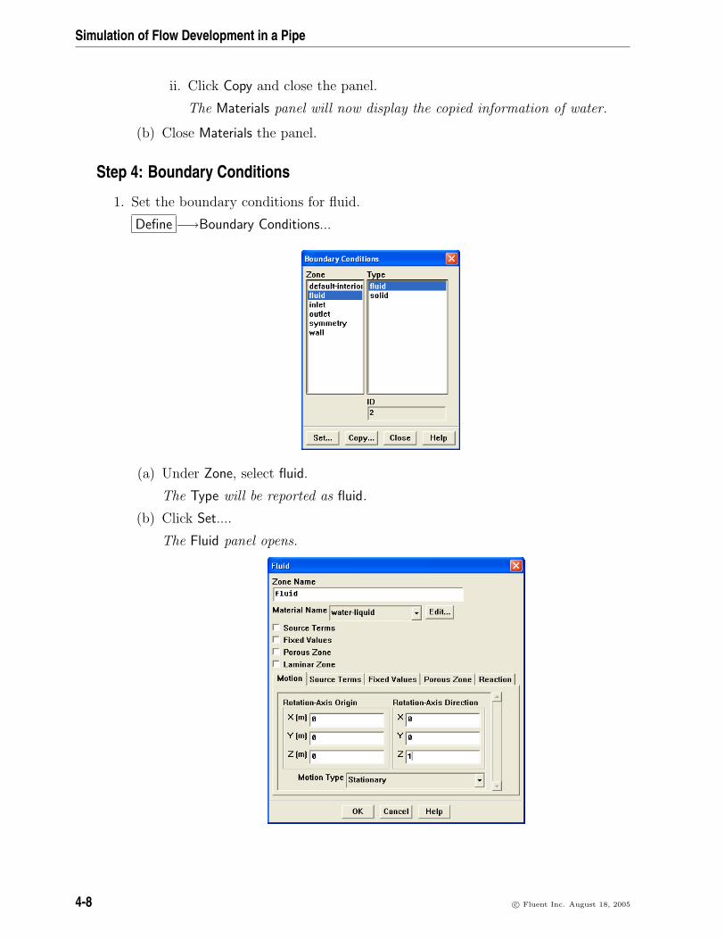
1. Set the boundary conditions for fluid.

Define −→Boundary Conditions...

(a) Under Zone, select fluid.

The Type will be reported as fluid.

(b) Click Set....

The Fluid panel opens.



i. Select water-liquid in the Material Name drop-down list.

ii. Click OK to accept the settings and close the panel.

2. Set the boundary conditions for inlet.

(a) Under Zone, select inlet.

The Type will be reported as velocity-inlet.

(b) Click Set....

The Velocity Inlet panel opens.

i. Specify a value of 0.015 for Velocity Magnitude (m/s).

The Reynolds number is defined as:

Re =U ×D × ρ

µ(4.1)

for fluid properties of water-liquid and to have Re = 15000, the velocityshould be set to 0.015 m/sec.

ii. Select Intensity and Hydraulic Diameter as Turbulence Specification Method.

iii. Specify a value of 4.8 for Turbulent Intensity.

Turbulent Intensity can be calculated as:

T.I. = 0.16×Re−1/8 (4.2)

iv. Specify a value of 1 for Hydraulic Diameter.

v. Click OK.



3. Set the boundary conditions for outlet.

(a) Under Zone, select outlet.

The Type will be reported as pressure-outlet.

(b) Click Set....

The Pressure Outlet panel opens.

Use the default value for gauge pressure since the outlet is maintained at at-mospheric pressure.

i. Select Intensity and Hydraulic Diameter as Turbulence Specification Method.

ii. Specify a value of 4.8 for Turbulent Intensity.

iii. Specify a value of 1 for Hydraulic Diameter.

These values of turbulence parameters will be used only if reverse flowoccurs at the outlet.

iv. Click OK.

Step 5: Solution

1. Set the solution controls.

Solve −→ Controls −→Solution...



(a) Select Second Order Upwind discretization schemes for Momentum, TurbulenceKinetic Energy, and Turbulence Dissipation Rate.

Since the flow is not very complex, you can use higher order discretizationschemes directly. In case of complex flows, it is recommended to obtain aconverged solution using first order schemes before switching to higher orderschemes.

(b) Click OK.

2. Initialize the flow.

Solve −→ Initialize −→Initialize...

(a) Set inlet in the Compute From drop-down list.

(b) Click Init and close the panel.

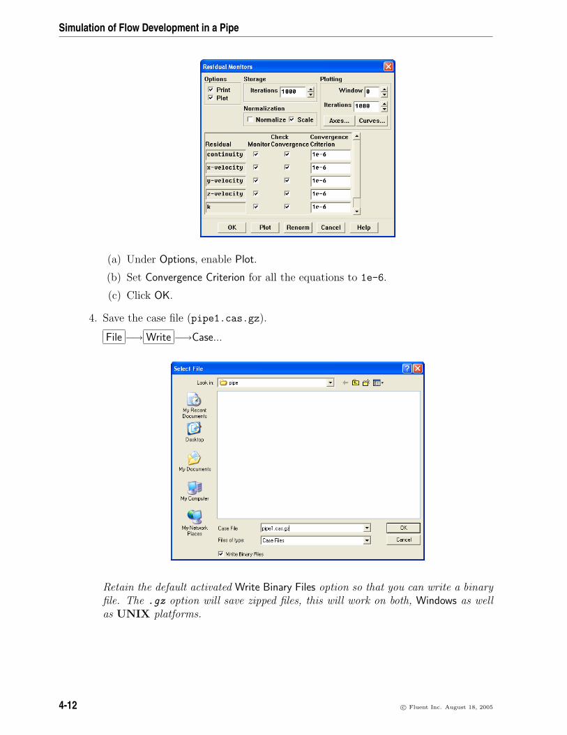
3. Enable plotting of residuals during the calculation and change the convergencecriteria.

Solve −→ Monitors −→Residuals...



(a) Under Options, enable Plot.

(b) Set Convergence Criterion for all the equations to 1e-6.

(c) Click OK.

4. Save the case file (pipe1.cas.gz).

File −→ Write −→Case...

Retain the default activated Write Binary Files option so that you can write a binaryfile. The .gz option will save zipped files, this will work on both, Windows as wellas UNIX platforms.



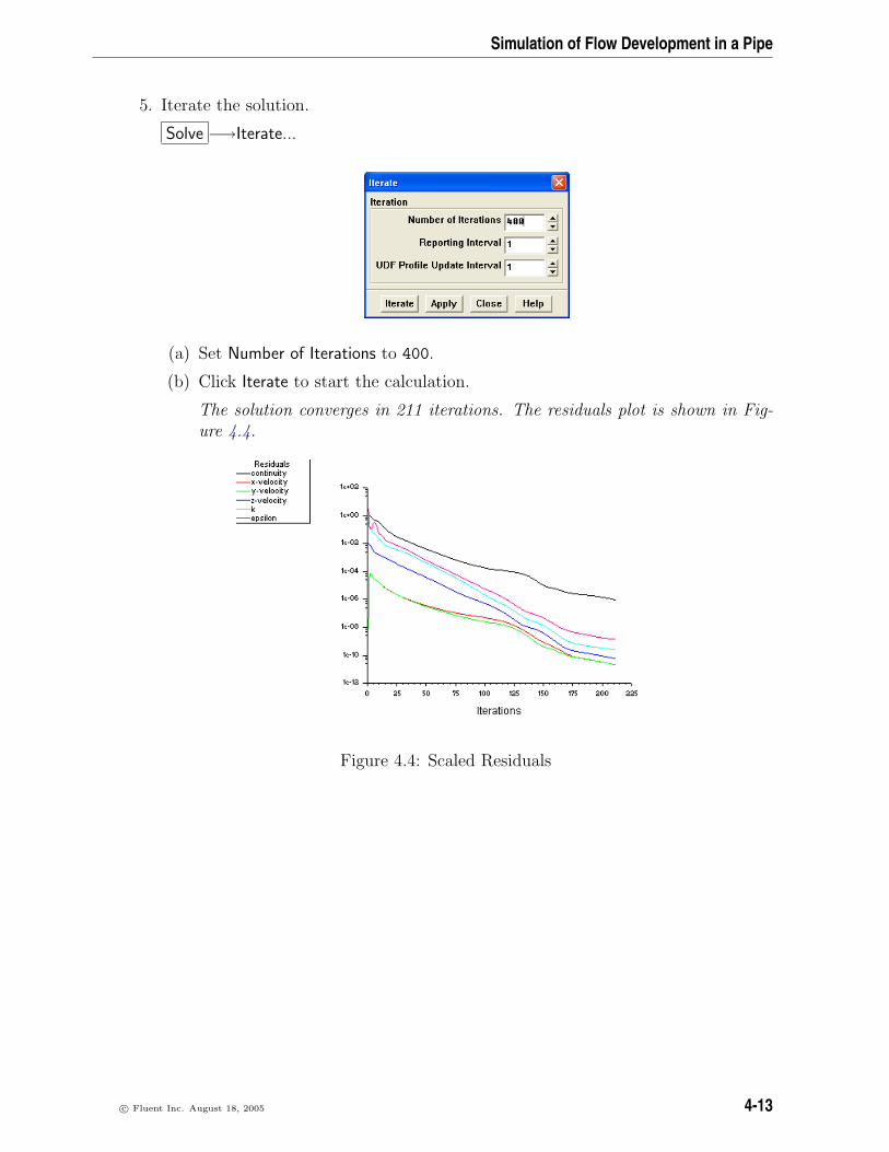
5. Iterate the solution.

Solve −→Iterate...

(a) Set Number of Iterations to 400.

(b) Click Iterate to start the calculation.

The solution converges in 211 iterations. The residuals plot is shown in Fig-ure 4.4.

Figure 4.4: Scaled Residuals



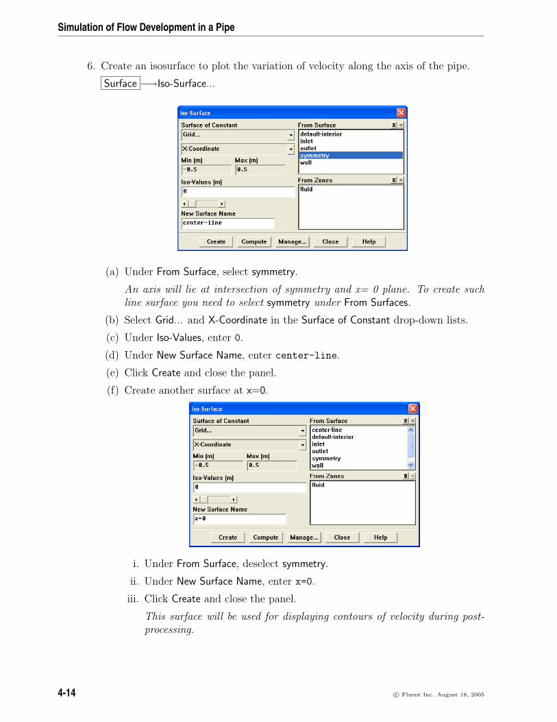
6. Create an isosurface to plot the variation of velocity along the axis of the pipe.

Surface −→Iso-Surface...

(a) Under From Surface, select symmetry.

An axis will lie at intersection of symmetry and x= 0 plane. To create suchline surface you need to select symmetry under From Surfaces.

(b) Select Grid... and X-Coordinate in the Surface of Constant drop-down lists.

(c) Under Iso-Values, enter 0.

(d) Under New Surface Name, enter center-line.

(e) Click Create and close the panel.

(f) Create another surface at x=0.

i. Under From Surface, deselect symmetry.

ii. Under New Surface Name, enter x=0.

iii. Click Create and close the panel.

This surface will be used for displaying contours of velocity during post-processing.



7. Create XY plots (Figure 4.5).

Plot −→XY Plot...

(a) Under Surfaces, select center-line.

(b) Set Plot Direction as X=0, Y=0, and Z=1.

(c) Select Velocity... and Z Velocity in the Y Axis Function drop-down list.

(d) Click Axes...

The Axes-Solution XY Plot panel opens.



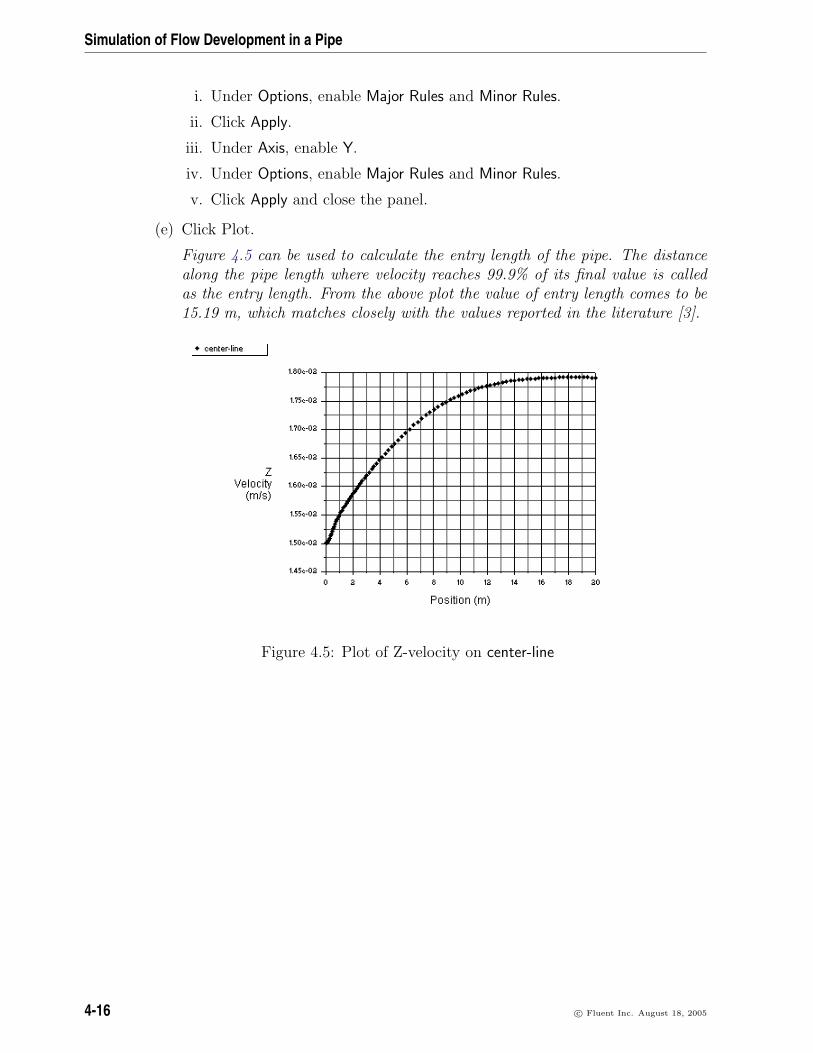
i. Under Options, enable Major Rules and Minor Rules.

ii. Click Apply.

iii. Under Axis, enable Y.

iv. Under Options, enable Major Rules and Minor Rules.

v. Click Apply and close the panel.

(e) Click Plot.

Figure 4.5 can be used to calculate the entry length of the pipe. The distancealong the pipe length where velocity reaches 99.9% of its final value is calledas the entry length. From the above plot the value of entry length comes to be15.19 m, which matches closely with the values reported in the literature [3].

Figure 4.5: Plot of Z-velocity on center-line



8. Calculation of friction factor at outlet.

Friction factor (f) is used to indicate the pressure drop in a pipe [2]. It is definedas:

f =∆P × 2

L× ρ× v2(4.3)

where,

∆P = Pressure drop along pipe length (L)D = Pipe diameterv = Average velocity in the pipe sectionρ = Fluid density

After balancing the pressure and shear forces the same expression takes the form:

f =8× τ

ρ× v2(4.4)

where, τ = Shear stress on the wall

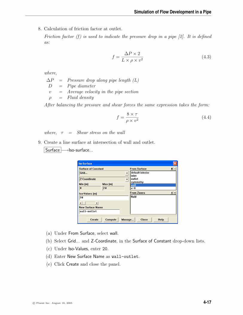
9. Create a line surface at intersection of wall and outlet.

Surface −→Iso-surface...

(a) Under From Surface, select wall.

(b) Select Grid... and Z-Coordinate, in the Surface of Constant drop-down lists.

(c) Under Iso-Values, enter 20.

(d) Enter New Surface Name as wall-outlet.

(e) Click Create and close the panel.



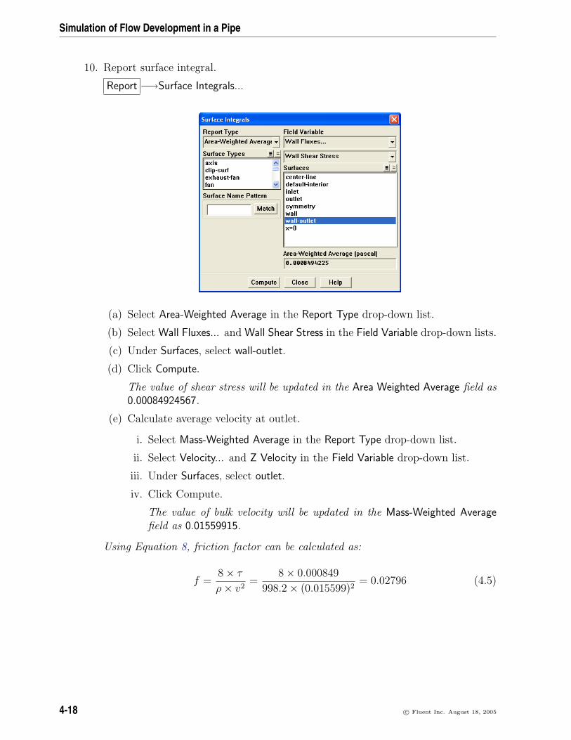
10. Report surface integral.

Report −→Surface Integrals...

(a) Select Area-Weighted Average in the Report Type drop-down list.

(b) Select Wall Fluxes... and Wall Shear Stress in the Field Variable drop-down lists.

(c) Under Surfaces, select wall-outlet.

(d) Click Compute.

The value of shear stress will be updated in the Area Weighted Average field as0.00084924567.

(e) Calculate average velocity at outlet.

i. Select Mass-Weighted Average in the Report Type drop-down list.

ii. Select Velocity... and Z Velocity in the Field Variable drop-down list.

iii. Under Surfaces, select outlet.

iv. Click Compute.

The value of bulk velocity will be updated in the Mass-Weighted Averagefield as 0.01559915.

Using Equation 8, friction factor can be calculated as:

f =8× τ

ρ× v2=

8× 0.000849

998.2× (0.015599)2= 0.02796 (4.5)



Step 8: Postprocessing

1. Display filled contours of wall Yplus (Figure 4.6).

Display −→Contours...

(a) Select Turbulence... and Wall Yplus in the Contours of drop-down lists.

(b) Under Surfaces, select wall.

(c) Under Options, enable Filled and disable Global Range.

(d) Click Display and close the panel.

The Yplus value for most of the domain is less than 5, except for the cells nearinlet, where it is slightly higher. This shows that enhanced wall treatment isacceptable as a wall function.

2. Enable the mirror plane to view the complete geometry.

Display −→Views...



Figure 4.6: Contours of Wall Yplus on wall

(a) Under Mirror Planes, select symmetry.

(b) Click Apply.

3. Display the velocity contours on surface x=0 (Figure 4.7).




(a) Select Velocity... and Velocity Magnitude in the Contours of drop-down lists.

(b) Under Surfaces, select x=0.

(c) Click Compute.

(d) Under Options, disable Auto Range.

(e) Specify Min as 0.0145 and retain Max as default.

(f) Click Display.

Figure 4.7 shows the development of velocity along the length of pipe.

Figure 4.7: Contours of Velocity Magnitude on x=0

4. Create another isosurface.

Surface −→Iso-surface...



(a) Select Grid... and Z-Coordinate in the Surface of Constant drop-down list.

(b) Under Iso-Values, specify a value of 0.1.

(c) Specify New Surface Name as z=0.1.

(d) Click Create and close the panel.

5. Display the velocity contours on surface z=0.1 (Figure 4.8).


(a) Select Velocity... and Velocity Magnitude in the Contours of drop-down lists.

(b) Under Surfaces, select z=0.1.

(c) Under Options, enable Auto Range.

(d) Under Options, enable Draw Grid.

Grid Display panel opens.



i. Deselect all the surfaces and select center-line.

ii. Click Display and close the panel.

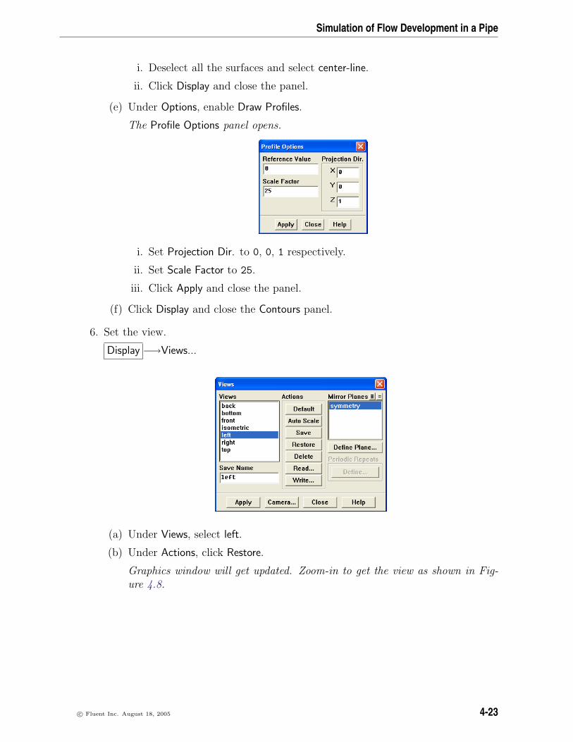
(e) Under Options, enable Draw Profiles.

The Profile Options panel opens.

i. Set Projection Dir. to 0, 0, 1 respectively.

ii. Set Scale Factor to 25.

iii. Click Apply and close the panel.

(f) Click Display and close the Contours panel.

6. Set the view.


(a) Under Views, select left.

(b) Under Actions, click Restore.

Graphics window will get updated. Zoom-in to get the view as shown in Fig-ure 4.8.



Figure 4.8: Profiles of Velocity Magnitude on z=0.1

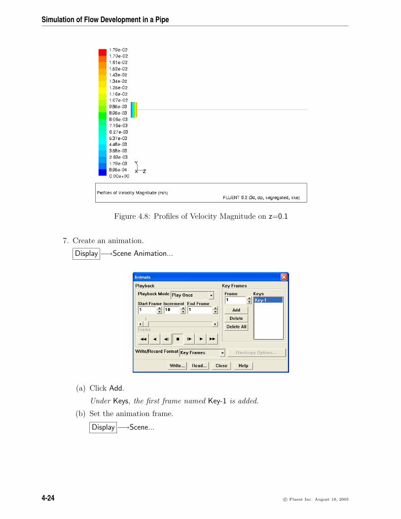
7. Create an animation.

Display −→Scene Animation...

(a) Click Add.

Under Keys, the first frame named Key-1 is added.

(b) Set the animation frame.

Display −→Scene...



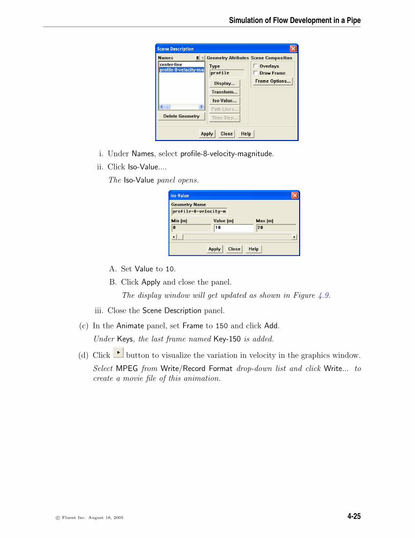
i. Under Names, select profile-8-velocity-magnitude.

ii. Click Iso-Value....

The Iso-Value panel opens.

A. Set Value to 10.

B. Click Apply and close the panel.

The display window will get updated as shown in Figure 4.9.

iii. Close the Scene Description panel.

(c) In the Animate panel, set Frame to 150 and click Add.

Under Keys, the last frame named Key-150 is added.

(d) Click button to visualize the variation in velocity in the graphics window.

Select MPEG from Write/Record Format drop-down list and click Write... tocreate a movie file of this animation.



Figure 4.9: Profiles of Velocity Magnitude–Frame 150

8. Create line surfaces to visualize the velocity vectors at different axial locations.

Surface −→Line/Rake...

(a) Set x0, y0, and z0 to 0.

(b) Set x1, y1, and z1 to 0, 0.5, and 0 respectively.

(c) Specify the New Surface Name as line=0.

(d) Click Create.

(e) Similarly, create 6 more surfaces with values of both, z0 and z1, set to 0.5, 1,1.5, 2, 2.5, and 3.

Name the surfaces accordingly, e.g., line=0.5, line=1 etc.



9. Display velocity vectors (Figure 4.10).

Display −→Vectors...

(a) Select Velocity in the Vectors of drop-down list.

(b) Select Velocity... and Velocity Magnitude in the Color by drop-down lists.

(c) Under Surfaces, select all the line/rake surfaces created in previous step.

(d) Under Options, enable Draw Grid.

Grid Display panel opens.

i. Under Surfaces, select all the line surfaces and x=0 surface.

ii. Under Edge Type, enable Outline.

iii. Click Display and close the panel.



Figure 4.10: Velocity Vectors

(e) Click Display and close the Vectors panel.

10. Change the view to get a closer view of velocity vectors.


(a) Under Actions, click Read....

This opens the Select File dialog box.

i. Select the view file and click OK.

(b) Under Views, select View and click Restore.

The display window will get updated as shown in Figure 4.11.

11. Save the case and data files (pipe2.cas.gz and pipe2.dat.gz).

File −→ Write −→Case & Data...



Figure 4.11: Velocity Vectors Close-up

Summary

This tutorial demonstrated the use of symmetry boundary condition to reduce the com-putational time without compromising the flow physics. Entry length and friction factorvalues obtained from FLUENT matches to those obtained from correlations. You alsolearned to use scene animation to visualize the development of flow field in the domain.

References

1. White Frank M., Viscous Fluid Flow, International Edition, McGraw-Hill, 1991, p423.

2. Schlichting H., Boundary-Layer Theory, 7th Edition, McGraw-Hill, 1979.

3. John M. Cimbala and Yunus A. Cengel, Fluid Mechanics Fundamentals and Ap-plications, 1st Edition, McGraw-Hill, 2005.

Exercises/ Discussions

1. Find the maximum Reynolds number for which current pipe length is sufficient toobtain a fully developed flow at outlet.

2. Compare the results using different wall functions.

3. Study the effect of roughness on the friction factor.

4. Change the velocity values and model laminar flow conditions.



5. Compare the results with pressure outlet boundary and outflow. How do theydiffer?

6. Conduct multiple runs by increasing the static pressure at the outlet. How does itinfluence the flow?

7. Simulate a periodic flow using the same mesh by creating a periodic zone usinginlet and outlet boundaries.

8. Apply a fully developed flow profile using profile files or user defined functions.

Links for Further Reading

• http://www.owlnet.rice.edu/∼mech372/handouts/viscous flows pipes.pdf

• http://www.engr.psu.edu/ce/hydro/hill/teaching/java/pipeflow.html

• http://www.cartage.org.lb/en/themes/Sciences/Physics/Mechanics/FluidMechanics/RealFluids/Laminar/Laminar.htm

• http://instruct1.cit.cornell.edu/courses/fluent/pipe2/index.htm


http://www.owlnet.rice.edu/~mech372/handouts/viscous_flows_pipes.pdf

http://www.engr.psu.edu/ce/hydro/hill/teaching/java/pipeflow.html

http://www.cartage.org.lb/en/themes/Sciences/Physics/Mechanics/FluidMechanics/RealFluids/Laminar/Laminar.htm

http://www.cartage.org.lb/en/themes/Sciences/Physics/Mechanics/FluidMechanics/RealFluids/Laminar/Laminar.htm

http://instruct1.cit.cornell.edu/courses/fluent/pipe2/index.htm

tutorial 4. simulation of flow development in a...

Documents