1 INTRODUCTION

Rivers and streams are usually in close association with vegetation. Natural rivers are mostly mean-dering and vegetation can occupy nearly every geomorphic position within the fluvial environ-ment. Vegetations in and near streams are sub-jected to varying flow stages that can inundate ve-getation during high flow events or leave it exposed during low flow events. Riparian vegeta-tion can play a critical role in the physical, eco-logical, and hydraulic functions of streams and rivers. Vegetation can affect the transport of wa-ter, sediment, and nutrients both within the chan-nel and to or between the riparian zones. The cha-racterization of not only the mean flow, but also turbulence structure and the associated transport processes in presence of vegetation, has received a lot of attention in the last decade (Lopez & Gar-cia, 2001). Thus, the characteristic of turbulent flow over a vegetation layer is one of the most fundamental topics in hydraulics of flow with ve-getation (Shimizu & Tsujimoto, 1994). The effect of marginal vegetation on flow resistance has been investigated for straight channels whereas

little is known of the effects for meandering chan-nels under either inbank or overbank flow condi-tions (James & Myers, 2001). The insight into flow distribution in straight as well as meandering main channels and the neighboring vegetated area is indispensable in river management.

Mean flow and turbulence characteristics of open channel flow with vegetation have been stu-died through laboratory experiments and numeri-cal computations. The k-ε model is the most commonly used two-equation model in engineer-ing and has proved to be a reliable tool in a wide variety of problems in hydraulic and environmen-tal engineering (Rodi, 1984). But none of the ex-isting turbulence models are truly universal and thus, each model needs to be tuned to specific flows (Choi & Kang, 2004). Using the k-ε model, Shimizu & Tsujimoto (1994) simulated the vertic-al distributions of the development of mean and turbulent flow structures. Lopez & Garcia (1997) also computed flow structures of vegetated open channel and compared the calculated results with their experimental ones. Choi & Kang (2004) ex-plained the performance of Reynolds stress model, algebraic stress model and the k-ε model for vege-

Turbulent Flow Structure in Meandering Vegetated Open Channel

F. Jahra, H. Yamamoto, F. Hasegawa & Y. Kawahara Department of Civil and Environmental Engineering, Hiroshima University, Higashi-Hiroshima, Japan

ABSTRACT: This study aims at revealing the flow structure of turbulent flows in a partially vegetated open channel where the width of vegetation zone changes as a sine-generated curve. The main objective of this paper is to gain insight into the mean flow field. Three-dimensional numerical simulation is carried out with the standard k-ε model to explore the distribution of mean velocity and turbulence structure in the main channel and the vegetation zone under both emergent and submerged vegetations. To capture the effect of vegetation on the flow, two different approaches have been adopted and the simulated results of these two approaches have been discussed. It is found that the second approach which has been devel-oped in the field of meteorology has wide range of application to detect flow structure. The numerical re-sults are compared against experimental observations in terms of mean velocities and Reynolds stresses, showing a fairly good agreement between simulated results and experimental results. The effect of change in vegetation density on flow structure is also discussed.

Keywords: Vegetated open channel,3D k-ε model, flow structure, Reynolds stresses, emergent and sub-merged vegetations

River Flow 2010 - Dittrich, Koll, Aberle & Geisenhainer (eds) - © 2010 Bundesanstalt für Wasserbau ISBN 978-3-939230-00-7

153

tated open channel flow simulation. Green (1992) modified a k-ε  model to examine the air flow through and over an isolated stand of widely-spaced trees with PHOENICS computer program, where he introduced additional source and sink terms to account for the effect of forest stand on the adjacent flow field. Using the similar source and sink terms Liu et al. (1996) also simulated the turbulent flow field downwind of forest edge.

The present study shows an application of the standard k-ε model to calculate the three-dimensional flow structure of partially vegetated open-channel flow. Two different approaches have been introduced, conventional approach widely used in the field of river engineering and another approach used in field of meteorology to compute the effect of vegetation on the flow field. The governing equation is both the short time and spatially averaged and the effect of individual roughness elements has been taken into account by an averaged local drag force. The computed re-sults have been compared with the laboratory measurement by the authors (Jahra et al., 2009) for two different vegetation densities and the values of model coefficients of both the models have been discussed.

2 EXPERIMENTAL SETUP

The experiments were conducted in a straight rec-tangular flume whose length and width are 22.0m and 1.82m, respectively. The channel has closed water supply system. Water is transported from downstream reservoir to the upstream reservoir by means of pipeline. The length of vegetation zone is 11.0m. The vegetation is idealized with wooden rigid cylinders of 3mm diameter and 5cm height. Three mean velocity components were measured by two-component electromagnetic current meters (both L-type and I-type) of 3mm diameter. Vege-tation zones were prepared on either side of the channel in meandering shape to suppress the large scale vortices that may develop in straight shaped vegetation zone. The meandering wavelength is 2.2m with the sinuosity of 1.10. There are five complete waves along the 11.0m long vegetated zones. Two cases of experiment were carried out: a shallow water case where vegetation was emer-gent and a deep water case with fully submerged vegetation. The measurements were carried out at the downstream section (about 8.35m from the tailgate) over half wave length at the points S1=12.55m, S2=12.85m, S3=13.1m, S4=13.35m and S5=13.65m. The equations of the interface curves are ( ) 435.02sin21.0 += lxZ π and

( ) 385.12sin21.0 += lxZ π . Figure 1 depicts the measurement sections in the partially vegetated meandering channel. Figure 2 shows the layout of the flume. The channel geometry and the flow conditions are summarized in Table 1. Flume measurement has been carried out with two differ-ent vegetation densities, λ=0.13/cm and 0.033/cm, respectively.

Table 1 Experimental condition for meandering channel.

3 MATHEMATICAL MODEL FORMULATION

The numerical calculations were conducted using the standard k-ε model. The computer code calcu-lates hydrodynamics for three dimensional geome-

Case

Bed slope

Dis-charge

Flow depth

Vegetation density Vegetation

condition [l/s] [cm] [1/cm]

A11/633 55.0

9.3 0.13 Sub-merged A2 8.3 0.033

B1 1/633 18.5

4.3 0.13 Emerged

B2 4.2 0.033

Figure 2. General layout of the meandering channel.

Figure 1. Measurement sections in meandering chan-nel (plan view).

Y=64.5cm

Y=162.5cm

Flow Y=43.5cm

Y=138.5cm

Y=19.5cm

Y=117.5cm

S2 S1 S3 S4 S5

154

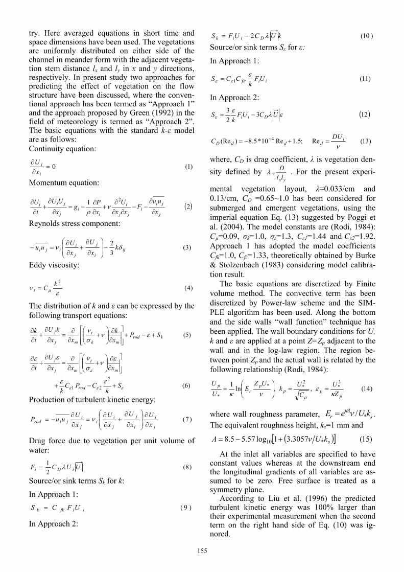
try. Here averaged equations in short time and space dimensions have been used. The vegetations are uniformly distributed on either side of the channel in meander form with the adjacent vegeta-tion stem distance lx and ly in x and y directions, respectively. In present study two approaches for predicting the effect of vegetation on the flow structure have been discussed, where the conven-tional approach has been termed as “Approach 1” and the approach proposed by Green (1992) in the field of meteorology is termed as “Approach 2”. The basic equations with the standard k-ε model are as follows: Continuity equation:

)1(0=∂∂

i

i

xU

Momentum equation:

( )21 2

j

jii

jj

i

ii

j

jii

xuu

Fxx

UxPg

xUU

tU

∂

∂−−

∂∂∂

+∂∂

−=∂

∂+

∂∂

νρ

Reynolds stress component:

)3(32

iji

j

j

itji k

xU

xUuu δν −⎟

⎟⎠

⎞⎜⎜⎝

⎛

∂

∂+

∂∂

=−

Eddy viscosity:

)4(2

εν μ

kCt =

The distribution of k and ε can be expressed by the following transport equations:

)5(krodmk

t

mj

j SPxk

xxkU

tk

+−+⎥⎥⎦

⎤

⎢⎢⎣

⎡

∂∂

⎟⎟⎠

⎞⎜⎜⎝

⎛+

∂∂

=∂

∂+

∂∂ εν

σν

Production of turbulent kinetic energy:

)7(j

i

i

j

j

it

j

ijirod x

Ux

UxU

xUuuP

∂∂

⎟⎟⎠

⎞⎜⎜⎝

⎛

∂

∂+

∂∂

=∂∂

−= ν

Drag force due to vegetation per unit volume of water:

)8(21 UUCF iDi λ=

Source/or sink terms Sk for k:

In Approach 1: )9(iifkk UFCS =

In Approach 2:

)10(2 kUCUFS Diik λ−= Source/or sink terms Sε for ε:

In Approach 1:

)11(1 iif UFk

CCS εεεε =

In Approach 2:

( )12323 ελε

ε UCUFk

S Dii −=

)13(Re;5.1Re10*5.8)(Re 4

νi

dddDDU

C =+−= −

where, CD is drag coefficient, λ is vegetation den-sity defined by

yxllD

=λ . For the present experi-

mental vegetation layout, λ=0.033/cm and 0.13/cm, CD =0.65~1.0 has been considered for submerged and emergent vegetations, using the imperial equation Eq. (13) suggested by Poggi et al. (2004). The model constants are (Rodi, 1984): Cµ=0.09, σk=1.0, σε=1.3, Cε1=1.44 and Cε2=1.92. Approach 1 has adopted the model coefficients Cfk=1.0, Cfε=1.33, theoretically obtained by Burke & Stolzenbach (1983) considering model calibra-tion result.

The basic equations are discretized by Finite volume method. The convective term has been discretized by Power-law scheme and the SIM-PLE algorithm has been used. Along the bottom and the side walls “wall function” technique has been applied. The wall boundary conditions for U, k and ε are applied at a point Z=Zp adjacent to the wall and in the log-law region. The region be-tween point Zp and the actual wall is related by the following relationship (Rodi, 1984):

)14(,,ln1 3*

2**

* ppp

pr

p

ZU

CUk

UZE

UU

κε

νκ μ

==⎟⎟⎠

⎞⎜⎜⎝

⎛=

where wall roughness parameter, sA

r kUeE */νκ= . The equivalent roughness height, ks=1 mm and

( )[ ] )15(3057.31log57.55.8 *10 skUA ν+−=

At the inlet all variables are specified to have constant values whereas at the downstream end the longitudinal gradients of all variables are as-sumed to be zero. Free surface is treated as a symmetry plane.

According to Liu et al. (1996) the predicted turbulent kinetic energy was 100% larger than their experimental measurement when the second term on the right hand side of Eq. (10) was ig-nored.

)6(2

21 εεε

ε

εε

ενσνεε

Sk

CPCk

xxxU

t

rod

m

t

mj

j

+−+

⎥⎥⎦

⎤

⎢⎢⎣

⎡

∂∂

⎟⎟⎠

⎞⎜⎜⎝

⎛+

∂∂

=∂

∂+

∂∂

155

Figure 4(a). U-velocity (cm/sec) contour of submerged vegetation for Case A1, at section S1, (i): Experimental result, (ii) Calculated result of Appr. 1, (iii) Appr. 2.

Green’s (1992) equation (Eq. (12)) for the source and sink term of ε has been modified in the present study as it is only an assumption where mixing length is considered locally invariant. An additional problem is that the second term on the right hand side considers only the reduction in the dissipation rate due to the reduction in k resulting from short-circuited energy cascade and does not include the increase in dissipation rate due to the reduction of turbulence mixing length (Liu et al., 1996). For present numerical model with meteoro-logical approach the second term on the right hand side of Eq. (12) has been modified by multiplying factor 0.47 to obtain fair agreement with the expe-rimental turbulent kinetic energy profile of Ghi-salberti (2007). The association between experi-mental result of U-velocity and turbulent kinetic energy profile with the calculated one by two ap-proaches are shown in Figure 3. A good agree-ment between two approaches is due to the similar distribution of tν although Approach 1 yields larger k and ε than Approach 2.

The present k-ε model is also found to repro-duce all the cases of both the series R and A, si-mulated by Shimizu & Tsujimoto (1994), using both approaches.

4 EXPERIMENTAL AND NUMERICAL RESULTS

Flume experiment was carried out for both the submerged and emerged cases with two different vegetation densities to get a clear vision of the flow structure and these experimental results are compared with the simulated results of both the approaches.

4.1 Mean Flow and Turbulent Stresses for Submerged Vegetation

Flow in meandering cannel has complex beha-viors. Figure 4(a) and Figure 4(b) show the U- ve-locity contours at the sections S1 and S5 respec-tively for both the experimental and calculated results of two different densities. It gives the qua-litative view of the cross-sectional flow structure.

Figure 3. Profile of U-velocity (left) and turbulent ki-

netic energy (right). The canopy height is 8.3cm, i.e. 0.21H.

Z/H

Z/H

U (cm/s) TKE (cm2/s2)

(i)

(ii)

(iii)

156

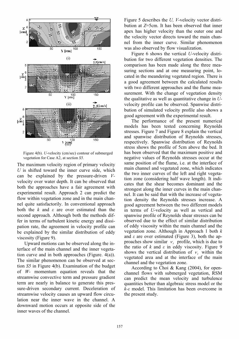
The maximum velocity region of primary velocity U is shifted toward the inner curve side, which can be explained by the pressure-driven V-velocity over water depth. It can be observed that both the approaches have a fair agreement with experimental result. Approach 2 can predict the flow within vegetation zone and in the main chan-nel quite satisfactorily. In conventional approach both the k and ε are over estimated than the second approach. Although both the methods dif-fer in terms of turbulent kinetic energy and dissi-pation rate, the agreement in velocity profile can be explained by the similar distribution of eddy viscosity (Figure 9).

Upward motions can be observed along the in-terface of the main channel and the inner vegeta-tion curve and in both approaches (Figure. 4(a)). The similar phenomenon can be observed at sec-tion S5 in Figure 4(b). Examination of the budget of W- momentum equation reveals that the streamwise convective term and pressure gradient term are nearly in balance to generate this pres-sure-driven secondary current. Deceleration of streamwise velocity causes an upward flow circu-lation near the inner wave in the channel. A downward motion occurs at opposite side of the inner waves of the channel.

Figure 5 describes the U, V-velocity vector distri-bution at Z=5cm. It has been observed that inner apex has higher velocity than the outer one and the velocity vector directs toward the main chan-nel from the inner curve. Similar phenomenon was also observed by flow visualization.

Figure 6 shows the vertical U-velocity distri-bution for two different vegetation densities. The comparison has been made along the three mea-suring sections and at one measuring point, lo-cated in the meandering vegetated region. There is a good agreement between the calculated results with two different approaches and the flume mea-surement. With the change of vegetation density the qualitative as well as quantitative change in U-velocity profile can be observed. Spanwise distri-bution of simulated velocity profile also shows a good agreement with the experimental result.

The performance of the present numerical models has been tested concerning Reynolds stresses. Figure 7 and Figure 8 explain the vertical and spanwise distribution of Reynolds stresses, respectively. Spanwise distribution of Reynolds stress shows the profile of 5cm above the bed. It has been observed that the maximum positive and negative values of Reynolds stresses occur at the same position of the flume, i.e. at the interface of main channel and vegetated zone, which indicates the two inner curves of the left and right vegeta-tion zone (considering half wave length). It indi-cates that the shear becomes dominant and the strongest along the inner curves in the main chan-nel. It can be said that with the increase of vegeta-tion density the Reynolds stresses increase. A good agreement between the two different models in terms of U-velocity as well as vertical and spanwise profile of Reynolds shear stresses can be observed due to the effect of similar distribution of eddy viscosity within the main channel and the vegetation zone. Although in Approach 1 both k and ε are over estimated (Figure 3), both the ap-proaches show similar tν profile, which is due to the ratio of k and ε in eddy viscosity. Figure 9 shows the vertical distribution of tν within the vegetated area and at the interface of the main channel and the vegetation zone.

According to Choi & Kang (2004), for open-channel flows with submerged vegetation, RSM can predict the mean velocity and turbulence quantities better than algebraic stress model or the k-ε model. This limitation has been overcome in the present study.

(i)

(ii)

(iii)

Figure 4(b). U-velocity (cm/sec) contour of submerged vegetation for Case A2, at section S5.

157

4.2 Mean Flow and Turbulent Stresses for Emergent Vegetation

The flow structure has also been observed for emergent vegetations with different densities. Like submerged vegetation, emerged case also shows a reasonable agreement with the calcula-tions by the two models. Figure 10 gives an image of the impact of change in vegetation density and also makes a qualitative comparison between la-boratory experiment and numerical simulations. It has been observed that both the models could nicely represent the presence of vegetation, though in Approach 1 mean velocity was underes-timated within the vegetation zone and overesti-mated in the main channel, especially near bed. This discrepancy can be explained by the concept of Choi & Kang (2004) and Tsujimoto et al. (1991), claiming that the drag-related weighting coefficients, Cfk and Cfε have to be tuned to specif-ic flows. For Approach 1 these model coefficients in the present study have been calibrated with the submerged vegetation. Hence in case of emergent vegetation, another set of model coefficients should be introduced to obtain better results. Re-garding drag-related weighting coefficients, Burke and Stolzenbach (1983) obtained theoretically Cfk = 1.0 and Cfε = 1.33. However, in numerical mod-eling, much smaller values for these coefficients were frequently used, for example, Cfk = 0.07 and

Cfε = 0.16 by Shimizu & Tsujimoto (1994), and Cfk = Cfε = 0.0 by Fischer-Antze et al. (2001). It can be seen that the drag-related coefficients hard-ly affect the streamwise mean velocity and Rey-nolds stress profiles. However, these coefficients seriously affect the turbulence kinetic energy as well as turbulence intensity profile. This limita-tion of 3D k-ε model is overcome when Approach 2 has been implemented. The advantage of this approach is that without implementation of differ-ent sets of drag related model coefficients it can predict the flow structure quite satisfactorily for different vegetation densities under submerged and emergent vegetation conditions. Figure 11 shows the spanwise distribution of Reynolds shear stress. Here it can be observed that with the in-crease of vegetation density the spanwise Rey-nolds stress increases in terms of positive and negative along the two inner apex of the meander-ing wave. The calculated result has a reasonable agreement with the measurement.

Spanwise distribution of U-velocity can be ob-served in Figure 12. Both the measured and calcu-lated points are located at 3.2 cm above the bed. Both the calculated results have a good agreement with the measured one. It can be observed that with the increase of vegetation density the veloci-ty slope at the interface of main channel and the vegetation zone becomes steeper.

Figure 5. Distribution of U, V velocity vector of submerged vegetation for CaseA1, Left: Experimental result, Right: Calculated result by Approach 1.

Figure 6. Experimental and calculated vertical distribution of U-mean velocity for submerged vegetation. 158

5 CONCLUSIONS

Flume experiments were carried out for turbulent open channel flows in the presence of meandering shaped vegetation under both submerged and emergent conditions. Numerical simulations were also performed with the standard k-ε model with the vegetation model in the transport equations for k and ε. The presence of vegetation has been in-troduced in the transport equations using two dif-ferent approaches; the conventional approach and an approach used in the field of meteorology. Comparisons between the measured data and the numerical results have led to the following find-ings. The present k- ε models can reproduce the mean

velocity field fairly well. The U-velocity increases in the main channel

and decreases in the vegetation as the vegeta-

tion density increases, resulting in the increase in the vertical and spanwise Reynolds stresses at the vegetation interface.

The maximum velocity region of U-velocity is shifted toward the inner wave due to the pres-sure driven secondary flows over water depth.

Streamwise convective term and the pressure gradient produce upward and downward mo-tions at the interface of the main channel and the vegetation zone.

The present numerical model with conventional approach to detect the presence of vegetation can predict the flow structure for submerged vegetation satisfactorily, with some discrepan-cy in case of emergent vegetation. This infers that another set of model coefficients, Cfk and Cfε is needed for better agreement with the measurement for emergent vegetation. This li-mitation has been overcome by introducing new source/sink term in transport equations. Hence Approach 2 can be used for wide variety of flow filed with vegetation without any im-plementation of drag related model coeffi-cients.

6 CONCLUSIONS

Flume experiments were carried out for turbulent open channel flows in the presence of meandering shaped vegetation under both submerged and

-u'w'(cm2/s2)Figure 7. Experimental and calculated vertical distribution of Reynolds stress profile for submerged vegetation.

Y(cm) Y(cm)

-u'v

'(cm

2 /s2 )

-u'v

'(cm

2 /s2 )

Y(cm) Figure 8. Experimental and calculated spanwise distribution of Reynolds stress profile for submerged vegetation.

-u'w'(cm2/s2)

Z(c

m)

-u'v

'(cm

2 /s2 )

Z(c

m)

-u'w'(cm2/s2)

Z(c

m)

Figure 9. Profile of vertical distribution of Eddy vis-cosity of Case A1.

Z(c

m)

Z(c

m)

Eddy Viscosity (cm2/s) Eddy Viscosity (cm2/s)

159

emergent conditions. Numerical simulations were also performed with the standard k-ε model with the vegetation model in the transport equations for k and ε. The presence of vegetation has been in-troduced in the transport equations using two dif-ferent approaches; the conventional approach and an approach used in the field of meteorology. Comparisons between the measured data and the numerical results have led to the following find-ings. The present k- ε models can reproduce the mean

velocity field fairly well. The U-velocity increases in the main channel

and decreases in the vegetation as the vegeta-tion density increases, resulting in the increase in the vertical and spanwise Reynolds stresses at the vegetation interface.

The maximum velocity region of U-velocity is shifted toward the inner wave due to the pres-sure driven secondary flows over water depth.

Streamwise convective term and the pressure gradient produce upward and downward mo-tions at the interface of the main channel and the vegetation zone.

The present numerical model with conventional approach to detect the presence of vegetation can predict the flow structure for submerged vegetation satisfactorily, with some discrepan-cy in case of emergent vegetation. This infers that another set of model coefficients, Cfk and Cfε is needed for better agreement with the measurement for emergent vegetation. This li-mitation has been overcome by introducing new source/sink term in transport equations. Hence Approach 2 can be used for wide variety of flow filed with vegetation without any im-plementation of drag related model coeffi-cients.

REFERENCES

Burke, R.W., Stolzenbach, K.D. 1983. Free surface flow through salt marsh grass. MIT-Sea Grant MITSG 83-16, Mass. Inst. of Technology, Cambridge, USA.

Choi, S., Kang, H. 2004. Reynolds stress modeling of vege-tated open-channel flows. Journal of Hydraulic Re-search, Vol.42, No.1, pp.3-11.

Fischer-Antze, T., Stoesser, T., Bates, P.B., Olsen, N.R. 2001. 3D numerical modelling of open-channel flow with submerged vegetation. Journal of Hydraulic Re-search, Vol.39, No.3,pp.303-310.

Ghisalberti, M. 2007. The impact of submerged canopies on open channel hydrodynamics. Fifth International Sym-posium on environmental Hydraulics, Tempe, Arizona, USA.

Green, S.R. 1992. Modelling turbulent air flow in a stand of widely-spaced trees. PHOENICS Journal of Computa-

tional Fluid Dynamics and Application, Vol.5, pp. 294-312.

Jahra, F., Yamamoto, H., Tsubaki, R., Kawahara, Y. 2009. Experimental study of mean velocity distributions in open channels with emergent and submerged vegetation. Journal of Applied Mechanics, Vol.12, pp. 663-672.

James, C.S., Myers, W.R.C. 2001. Conveyance of meander-ing channel with marginal vegetation. Proceedings of the Institution of Civil Engineers. Water, Maritime and Energy, Vol.148, pp. 97-106.

Liu, J., Chen, J.M., Black, T.A., Novak, M.D. 1996. E-ε modelling of turbulent air flow downwind of a model forest edge. Boundary-Layer Meteorology, Kluwer Aca-demic Publishers, Netherlands, Vol.77, pp.21-44.

Lopez, F., Garcia, M. 2001. Mean flow and turbulence structure of open-channel flow through non-emergent vegetation. Journal of Hydraulic Engineering, Vol.127, No.5, pp.392-402.

Lopez, F., Garcia, M. 1997. Open-channel flow through simulated vagetation: Turbulence modeling and sedi-ment transport. Wetlands Res. Program Rep. WRP-CP-10, U.S. Army Corps of Engineers, Washington, D.C.

Poggi, D., Porporato, A., Ridolfi, L., Albertson, J.D., Katul, G.G. 2004. The effect of vegetation density on canopy sub-layer turbulence. Boundary-Layer Meteorology. Vol.111.pp.565-587.

Rodi, W. 1984. Turbulence models and their applications in hydraulics. A state-of-art review, International Associa-tion for Hydraulic Research, Delft, The Netherlands.

Shimizu, Y., Tsujimoto, T, 1994. Numerical analysis of tur-bulent open-chgannel flow over a vegetation layer using a k-ε turbulence model. Journal of Hydroscience and Hydraulic Engineering, Vol.11, No.2, pp.57-67.

Tsujimoto, T., Kitamura, T., Okada, T. 1991. Turbulent structure of flow over rigid vegetation-covered bed in open channels. KHL Progressive Rep.1, Hydr. Lab., Ka-nazawa Univerdity, Japan.

160

Figure 10(a). U-velocity (cm/sec) contour of emergent vegetation for Case B1, at section S5. Left: Experimental result, Middle: Calculated result of Approach1, Right: Calculated result of Approach 2.

Figure 11 Experimental and calculated spanwise distribution of Reynolds stress profile for emergent vegetation.

Figure 12. Experimental and calculated spanwise distribution of U-velocity profile for emergent vegetation.

Figure 10(b). U-velocity (cm/sec) contour of emergent vegetation for Case B2, at section S5. Left: Experimental result, Middle: Calculated result of Approach1, Right: Calculated result of Approach 2.

U(c

m/s

)

Y(cm)

-u'v

'(cm

2 /s2 )

Y(cm)

-u'v

'(cm

2 /s2 )

Y(cm)

Y(cm)

U(c

m/s

)

Y(cm)

-u'v

'(cm

2 /s2 )

Y(cm)

161