Turbine Tip Clearance Control Using Fluidic Oscillators

By

Aaron R. Burns

Submitted to the graduate degree program in Aerospace Engineering and the

Graduate Faculty of the University of Kansas in partial fulfillment of the

requirements for the degree of Master of Science.

________________________________

Chairperson Dr. Saeed Farokhi

________________________________

Dr. Ray Taghavi

________________________________

Dr. Zhongquan Charlie Zheng

Date Defended: May 8, 2015

ii

The Thesis Committee for Aaron R. Burns

certifies that this is the approved version of the following thesis:

Turbine Tip Clearance Control Using Fluidic Oscillators

________________________________

Chairperson Dr. Saeed Farokhi

Date approved: May 8, 2015

iii

ABSTRACT

This study investigates the impact to power generation and efficiency by injecting flow into the

tip clearance region of a gas turbine rotor. New to this design is using a fluidic oscillator as the

jet source for the injection instead of a circular jet. The fluidic oscillator in this study is a

bistable, vent fed oscillator. It creates a sweeping jet at its exit with a primary frequency in the 1

kHz to10 kHz range dependent on the supply mass flow and internal geometry. In this study,

rotor tip clearance in the range of 2% to 10% of blade span is investigated for the flowing rotor

tip types: flat tip, 2 and 4 fluidic oscillators on a flat tip, circle jets on a flat tip, squealer tip, 4

fluidic oscillators on a squealer tip, and circle jets on a squealer tip.

This study was performed using the commercial CFD package STAR-CCM+. A polyhedral

mesh was used for enhanced accuracy and reduced compute times. The significant flow models

used were implicit unsteady, k-e turbulence, and real air. Also the turbine rotor was rotated

about the z-axis (cylindrical) to simulate a real rotor. Only two blades of the entire rotor were

simulated using periodic boundary conditions to simulate the rest of the rotor wheel.

The tips with 4 fluidics showed the largest efficiency gain of 2% to 3% over the flat tip, 0% to

1% over the squealer tip, and about 1% over the circle jet tips. The 4 fluidic tips produced nearly

twice as power per orifice as compared to the circle jet tips. The 2 fluidic tip had an efficiency

gain of about 1% over the flat tip, an efficiency loss compared to the squealer tip, and 0% to

0.5% gain over the circle jet tips. The 2 fluidic tip produced 12% to 40% more power than the

circle jet tips. The two 4 fluidic tips and the 2 fluidic tip created more turbine power that in took

the compressor to make the supply air. However, when compared to the power production of the

squealer tip, almost all tip configurations did not produce more power than it took to make the

supply air.

iv

ACKNOWLEDGEMENTS

This thesis is the result of research work at the Department of Aerospace Engineering of the

University of Kansas. I would like to express my gratitude towards my advisor, Dr. Saeed

Farokhi for his guidance and support and sharing his deep knowledge of jet propulsion. I would

like to thank the two other members of my committee, Drs. Ray Taghavi and Zhongquan Charlie

Zheng, for taking the time to review this thesis and provide comments and suggestions.

I am thankful for Drs. Ameri and Vikram for hosting me at NASA Glenn Research Center in

Cleveland, OH. Visiting all the different research laboratories and speaking with the researchers

themselves was an experience I will never forget.

Lastly, I would like to thank my wife, Alexandra, and both our families for your constant support

and prayers over these last few years. I would not have it through graduate school without you. I

love you all.

v

TABLE OF CONTENTS

ABSTRACT ..............................................................................................................................iii

ACKNOWLEDGEMENTS ............................................................................................................iv

LIST OF FIGURES .....................................................................................................................vi

NOMENCLATURE .....................................................................................................................viii

1. INTRODUCTION .................................................................................................................1

2. LITERATURE REVIEW ........................................................................................................2

2.1. SECONDARY FLOWS...................................................................................................3

2.2. TURBOMACHINERY UNSTEADY FLOW INTERACTION .................................................5

2.3. TURBOMACHINERY LOSSES .......................................................................................7

2.4. TIP CLEARANCE LOSSES ............................................................................................8

2.5. FLUIDIC OSCILLATOR ................................................................................................12

3. COMPUTATIONAL SETUP ...................................................................................................15

3.1. STAR-CCM+ ...............................................................................................................15

3.2. POLYHEDRAL VS. TETRAHEDRAL MESHES.................................................................15

3.3. MESH SETTINGS AND PHYSICS MODELS ....................................................................19

4. RESULTS ...........................................................................................................................24

4.1. MASS FLOW INJECTION .............................................................................................24

4.1.1. TIP LEAKAGE VORTEX .....................................................................................25

4.1.2. ROTOR WAKE ...................................................................................................30

4.2. EFFECTS OF CLEARANCE HEIGHT ..............................................................................31

4.3. ROTOR EFFICIENCY ...................................................................................................36

4.4. ROTOR POWER ...........................................................................................................37

5. CONCLUSIONS ...................................................................................................................40

5.1. GENERAL CONCLUSIONS ...........................................................................................40

5.2. FOR FURTHER STUDY ................................................................................................41

6. REFERENCES .....................................................................................................................42

vi

LIST OF FIGURES

1.1 PW1000G HIGH-BYPASS GEARED TURBOFAN ENGINE ...........................................................1

1.2 TURBINE ROTOR SHOWING FLUIDIC OSCILLATOR ORIENTATION ............................................3

2.1.1 DEFINITION SKETCH OF SECONDARY FLOW GENERATION IN A TURBINE BLADE ROW ..........4

2.1.2 DEFINITION SKETCH OF VORTEX STRUCTURE IN ENDWALL REGION ....................................5

2.2.1 BLADE WAKE CHOPPING .....................................................................................................7

2.4.1 ENDWALL LOSS DEVELOPMENT FOR UNSHROUDED TURBINE ROTOR ................................10

2.4.2 COMMON TURBINE ROTOR TIP CONFIGURATIONS .............................................................12

2.4.3 CD OF COMMON TURBINE ROTOR TIPS VERSUS FLAT TIP ..................................................12

2.5.1 CLASSICAL FLUIDIC OSCILLATOR DESIGNS .......................................................................14

2.5.2 SCHEMATIC SKETCH OF A) SYMMETRIC BISTABLE AND B) ASYMMETRIC MONOSTABLE

OSCILLATORS ............................................................................................................................15

3.2.1 A) TETRAHEDRAL MESH AND B) POLYHEDRAL MESH AT TURBINE ROTOR .........................18

3.2.2 TETRAHEDRAL AND POLYHEDRAL MESH SOLUTION OF THE WATER JACKET ....................19

3.2.3 CONVERGENCE OF PRESSURE IN WATER JACKET ...............................................................20

3.3.1 TURBINE ROTOR EXIT TOTAL PRESSURE VERSUS POLYHEDRAL CELL COUNT ....................21

3.4.1 GEOMETRY BOUNDARY CONDITIONS ................................................................................23

3.4.2 FLUIDIC OSCILLATOR CAD GEOMETRY ............................................................................24

3.4.3 CONVERGENCE OF X VELOCITY AT FLUIDIC EXIT ..............................................................24

3.4.4 CONVERGENCE OF Y VELOCITY AT FLUIDIC EXIT ..............................................................25

3.4.5 FFT OF X VELOCITY AT FLUIDIC EXIT ...............................................................................25

3.4.6 FFT OF Y VELOCITY AT FLUIDIC EXIT ...............................................................................26

3.4.7 PRESSURE CONVERGENCE ................................................................................................26

4.1.1.1 TURBULENCE INTENSITY FOR 5% FLAT TIP ....................................................................27

4.1.1.2 TURBULENCE INTENSITY FOR 5% TIP WITH 4 FLUIDICS .................................................28

4.1.1.3 TURBULENCE INTENSITY FOR 5% SQUEALER TIP ...........................................................28

4.1.1.4 TURBULENCE INTENSITY FOR EACH TIP CONFIGURATION AT ROTOR EXIT ......................29

4.1.1.5 EXIT FLOW ANGLE FOR NON-RECESSED TIPS AT ROTOR EXIT .........................................30

4.1.1.6 EXIT FLOW ANGLE FOR SQUEALER TIPS AT ROTOR EXIT .................................................30

vii

4.1.1.7 TOTAL PRESSURE COEFFICIENT AT ROTOR EXIT .............................................................31

4.1.2.1 AXIAL VELOCITY AT ROTOR EXIT ..................................................................................32

4.1.2.2 FLOW ANGLE AT ROTOR EXIT ........................................................................................33

4.2.1 AXIAL VELOCITY FOR INCREASING TIP CLEARANCES AT ROTOR EXIT ...............................34

4.2.2 AXIAL VELOCITY COMPARISON TO A 5% FLAT TIP AT ROTOR EXIT ...................................34

4.2.3 EXIT FLOW ANGLE FOR INCREASING TIP CLEARANCES AT ROTOR EXIT .............................35

4.2.4 EXIT FLOW ANGLE COMPARISON TO A 5% FLAT TIP AT ROTOR EXIT .................................36

4.2.5 TURBULENCE INTENSITY FOR INCREASING TIP CLEARANCE AT ROTOR EXIT .....................37

4.2.6 TURBULENCE INTENSITY COMPARISON TO A 5% FLAT TIP AT ROTOR EXIT .......................37

4.3.1 EFFICIENCY FOR TIP CONFIGURATIONS AT ROTOR EXIT ....................................................38

4.4.1 POWER DIFFERENCE COMPARED TO FLAT TIP POWER PRODUCTION ..................................40

4.4.2 POWER DIFFERENCE COMPARED TO POWER REQUIRED FOR INJECTED ..................................

AIR AGAINST FLAT TIP ......................................................................................................40

4.4.3 POWER DIFFERENCE COMPARED TO SQUEALER TIP POWER PRODUCTION ..........................41

4.4.4 POWER DIFFERENCE COMPARED TO POWER REQUIRED FOR INJECTED ..................................

AIR AGAINST SQUEALER TIP..............................................................................................42

viii

NOMENCLATURE

c ...................................................... CONVECTIVE SPEED .............................................................. m/s

𝑐𝑝 .................................... SPECIFIC HEAT AT CONSTANT PRESSURE ........................................... J/kgK

ε ...................................................... EFFICIENCY FACTOR ................................................................. --

f ............................................................ FREQUENCY ..................................................................... Hz

𝛾 ................................................. RATIO OF SPECIFIC HEATS ............................................................. --

h............................................................. ENTHALPY .................................................................. kJ/kg

∆�̇� ..................................................... ENTHALPY FLUX ...................................................kJ/kg*(kg/s)

l ......................................................... LENGTH SCALE ................................................................... m

M ....................................................... MACH NUMBER .................................................................... --

�̇� ...................................................... MASS FLOW RATE ............................................................... kg/s

𝜂 ............................................... AERODYNAMIC EFFICIENCY ........................................................... --

P ............................................................... POWER .......................................................................... W

p....................................................... STATIC PRESSURE .................................................................Pa

𝑝𝑡 ...................................................... TOTAL PRESSURE ..................................................................Pa

R .........................................................GAS CONSTANT.............................................................. J/kgK

s .............................................................. ENTROPY ...................................................................... J/K

T ................................................... STATIC TEMPERATURE ............................................................... K

𝑇𝑡 .................................................. TOTAL TEMPERATURE ............................................................... K

�̅�................................................... REDUCED FREQUENCY ............................................................... --

ACRONYMS

FAST FOURIER TRANSFORM ......................................................................................................... FFT

HIGH CYCLE FATIGUE ................................................................................................................ HCF

HIGH PRESSURE TURBINE ........................................................................................................... HPT

LOW PRESSURE TURBINE ............................................................................................................ LPT

OVER-THE-TIP LEAKAGE ............................................................................................................ OTL

1

1. Introduction

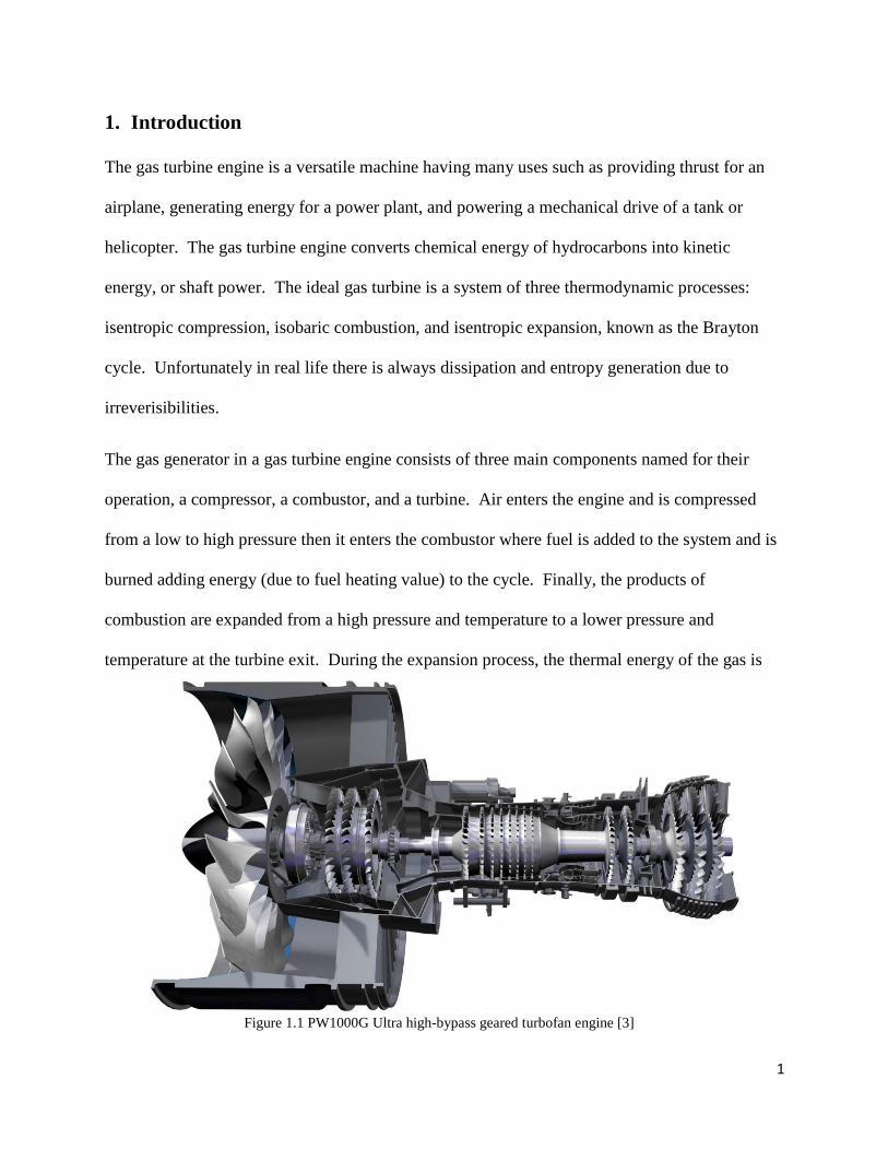
The gas turbine engine is a versatile machine having many uses such as providing thrust for an

airplane, generating energy for a power plant, and powering a mechanical drive of a tank or

helicopter. The gas turbine engine converts chemical energy of hydrocarbons into kinetic

energy, or shaft power. The ideal gas turbine is a system of three thermodynamic processes:

isentropic compression, isobaric combustion, and isentropic expansion, known as the Brayton

cycle. Unfortunately in real life there is always dissipation and entropy generation due to

irreverisibilities.

The gas generator in a gas turbine engine consists of three main components named for their

operation, a compressor, a combustor, and a turbine. Air enters the engine and is compressed

from a low to high pressure then it enters the combustor where fuel is added to the system and is

burned adding energy (due to fuel heating value) to the cycle. Finally, the products of

combustion are expanded from a high pressure and temperature to a lower pressure and

temperature at the turbine exit. During the expansion process, the thermal energy of the gas is

Figure 1.1 PW1000G Ultra high-bypass geared turbofan engine [3]

2

partly converted into mechanical energy which is used to power the compressor and other

subsystems. Today, the primary uses of gas turbines is to generate electrical power in power

plants and to create thrust/lift and other propulsive forces for aircraft. The gas turbine industry is

a very competitive market in all applications. Therefore, an engine’s figures of merit are

efficiency, power density, manufacturing and operation costs, and emissions. A modern ultra-

high bypass geared turbofan engine, PW1000G, is shown in Figure 1.1.

The turbine section of the engine consists of stages of stationary and rotating blade rows. The

stator blade row, which is called a nozzle, imparts swirl or angular velocity to the axial flow,

thereby imparting angular momentum to the fluid. Directly after the nozzle blade row is the

rotor blade row which converts the thermal energy of the flow into mechanical energy by

partially/fully absorbing the angular momentum that the nozzle imparted to the fluid. Since the

turbine is a complex mechanical system, it has numerous generating mechanisms. The goal of

turbine research is to identify and reduce the impact of these losses thus improving turbine

efficiency. The current work investigates a new system to control the primary loss source in

high-pressure turbines (HPT), namely rotor tip clearance loss.

The section of the turbine that is focused on here, as noted earlier, is the clearance region

between the tip of the rotor and the casing. Up to one third of the losses present in a high-

pressure turbine are attributed to the tip leakage flow. Reducing the clearance height would

indeed lessen the tip leakage loss. It poses a challenging problem however since tip clearance

changes with the thermal and mechanical loads on the engine during its operation (in aircraft,

from takeoff to climb, cruise, descent and landing). This requires an alternate method of sealing

the clearance. This study investigates the novel method to reduce the tip leakage flow by sealing

3

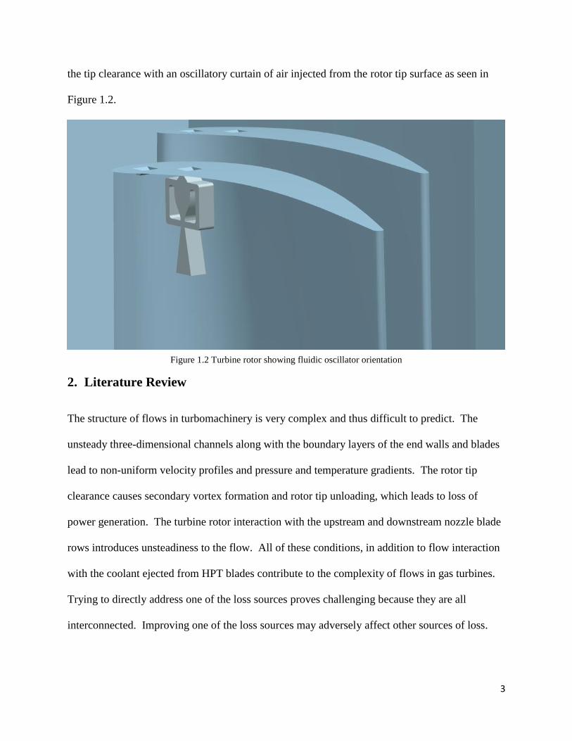
the tip clearance with an oscillatory curtain of air injected from the rotor tip surface as seen in

Figure 1.2.

2. Literature Review

The structure of flows in turbomachinery is very complex and thus difficult to predict. The

unsteady three-dimensional channels along with the boundary layers of the end walls and blades

lead to non-uniform velocity profiles and pressure and temperature gradients. The rotor tip

clearance causes secondary vortex formation and rotor tip unloading, which leads to loss of

power generation. The turbine rotor interaction with the upstream and downstream nozzle blade

rows introduces unsteadiness to the flow. All of these conditions, in addition to flow interaction

with the coolant ejected from HPT blades contribute to the complexity of flows in gas turbines.

Trying to directly address one of the loss sources proves challenging because they are all

interconnected. Improving one of the loss sources may adversely affect other sources of loss.

Figure 1.2 Turbine rotor showing fluidic oscillator orientation

4

One method of improving turbine efficiency is to have jets blow directly into the tip clearance

region of the rotor to mitigate the tip leakage flow.

2.1. Secondary Flows

A secondary flow, simply put, is any flow structure that forms in a channel which is not aligned

with the primary flow. Most secondary flows are caused by the vortex stretching in the endwall

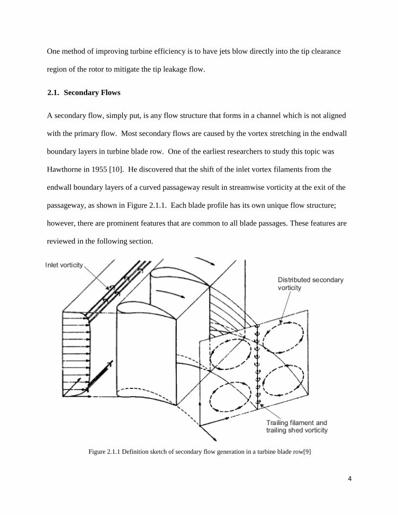
boundary layers in turbine blade row. One of the earliest researchers to study this topic was

Hawthorne in 1955 [10]. He discovered that the shift of the inlet vortex filaments from the

endwall boundary layers of a curved passageway result in streamwise vorticity at the exit of the

passageway, as shown in Figure 2.1.1. Each blade profile has its own unique flow structure;

however, there are prominent features that are common to all blade passages. These features are

reviewed in the following section.

Figure 2.1.1 Definition sketch of secondary flow generation in a turbine blade row[9]

5

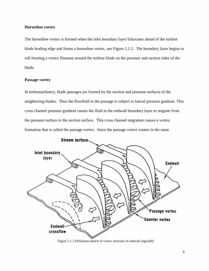
Horseshoe vortex

The horseshoe vortex is formed when the inlet boundary layer bifurcates ahead of the turbine

blade leading edge and forms a horseshoe vortex, see Figure 2.1.2. The boundary layer begins to

roll forming a vortex filament around the turbine blade on the pressure and suction sides of the

blade.

Passage vortex

In turbomachinery, blade passages are formed by the suction and pressure surfaces of the

neighboring blades. Thus the flowfield in the passage is subject to lateral pressure gradient. This

cross channel pressure gradient causes the fluid in the endwall boundary layer to migrate from

the pressure surface to the suction surface. This cross channel migration causes a vortex

formation that is called the passage vortex. Since the passage vortex rotates in the same

Figure 2.1.3 Definition sketch of vortex structure in endwall region[8]

6

direction as the horseshoe vortex, the two vortices tend to coalesce into one larger vortex at the

exit of the blade passage.

Corner vortex

A corner vortex is a counter rotating secondary vortex generated by a sufficiently strong primary

vortex influencing trapped fluid near a corner. In the case of a turbine, the migration of the

passage vortex to the suction surface collects fluid into the corner formed by the blade wall and

the endwall. The passage vortex along with the horseshoe vortex generate a counter rotating

corner vortex to form due to this strong crossflow impingement. Since the vortex is located in

the endwall suction side corner [11], it reduces the amount of overturning near endwalls [12].

2.2. Turbomachinery Unsteady Flow Interaction

The fact that turbomachinery has rotating and stationary blade rows along with non-uniform flow

field causes unsteadiness in the blade passages. Unsteadiness is partly random on the scale of

turbulence time scale and dominated by the blade passing frequency. A non-dimensional

parameter used to determine how unsteady a flow field is, the reduced frequency �̅� is defined as

the ratio of two time scales, convective time scale and the disturbance or fluctuation time scale:

�̅� =

𝑐 𝑙⁄

1 𝑓⁄ (2.2.1)

The flow is characterized as quasi-steady when �̅� ≪ 1, combined unsteady and quasi-steady

when �̅� ≅ 1, and highly unsteady when �̅� ≫ 1. According to Behr [13] in the case of a turbine,

�̅� ≅ 2 indicating a significant contribution of unsteady effects to the flow field.

Potential flow interaction

7

Each blade row in a gas turbine engine, in the absence of viscosity, interacts with each other,

within irrotational or potential fields. Neighboring potential fields interact in an unsteady

manner due to the relative motion of the blade rows. This interaction, even in the inviscid limit,

is a source of loss generation [14], and produces noise and blade vibration. Potential fields of

blade rows stretch in the upstream and downstream direction and are characterized by

exponential decay.

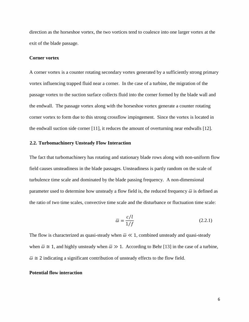
Wake-blade interaction

An isolated blade row creates viscous wake at its blades' trailing edge. This periodic wake

moves downstream and gets chopped by the following blade row creating a series of wake pieces

[15]. As the wake moves in the blade channel, it becomes stretched due the higher velocity near

the suction side and the lower velocity on the pressure side of the channel (see Figure 2.2.1).

This migration of wake fluid concentrates the wake on the suction side with a tail reaching back

to the pressure side.

Figure 2.2.1 Blade wake chopping [1]

8

Vortex interaction

In highly loaded low pressure turbines (LPT), the effect of upstream wake and blade interaction

on unsteady loads is important. However, in the high pressure turbine (HPT), low aspect ratio

environment of the first turbine rotor, secondary flow interaction dominates compared to

upstream wake interaction. In this region, the endwall vortices occupy a large portion of the

channel span. Endwall vortices wrap around downstream blades and are not chopped like

upstream wakes. The warped vortices tend to join and coalesce with the new vortices being

generated by the downstream blade.

2.3. Turbomachinery Losses

The losses in turbomachinery are categorized into three different generators: profile loss, endwall

loss, and leakage loss. They are named based on the source of the loss; however, the mechanics

for each loss generator are rarely independent of one another. A common method to define the

loss in a fluid flow system is by means of entropy generation. Entropy a thermodynamic

property describes the random statue of fluid and thus the irreversibility of a process. Thus any

entropy that is generated by a system can only be accumulated. In the case of turbomachines,

entropy is well-suited to measure loss since it is independent of frame of reference of the

observer. Entropy can be defined using the ratios of local and reference temperatures and

pressures following the Gibbs’ equation as

𝑠 − 𝑠𝑟𝑒𝑓 = 𝑐𝑝 ln (

𝑇

𝑇𝑟𝑒𝑓) − 𝑅𝑙𝑛 (

𝑝

𝑝𝑟𝑒𝑓) (2.3.1)

Denton [16] defines three primary entropy generating processes present in turbomachines:

1.) Viscous friction caused in boundary layers or free shear layers.

9

2.) Heat Transfer in casing and blade cooling.

3.) Non-equilibrium processes such as shockwaves.

2.4. Tip Clearance Losses

The tip clearance between the blade and the casing of an unshrouded turbine rotor introduces a

leakage flow to the turbine stage which has adverse effects on performance. The leakage flow

does not provide useful work as it essentially bypasses the rotor and thus experiences a greatly

reduced turning compared to the main flow. Also, the torque of each rotor blade is reduced due

to the shorter blade length.

Bindon [6] experimentally studied the mechanisms for loss in the tip region of an unshrouded

turbine rotor. He identified three groups of overall loss for the clearance region:

Secondary and endwall loss. The endwall loss is partially caused by skin friction shear stress on

the endwall across the length of the clearance passage. The secondary flow loss pertains to all

other three dimensional losses, which exclude the blade profile loss.

Internal gap and shear loss covers losses due to viscous friction of the flow inside the clearance

passage. The primary drivers of this loss are the relative motion of the casing wall and the blade

tip surface and the momentum difference of the leakage jet and the separated flow in the

clearance region.

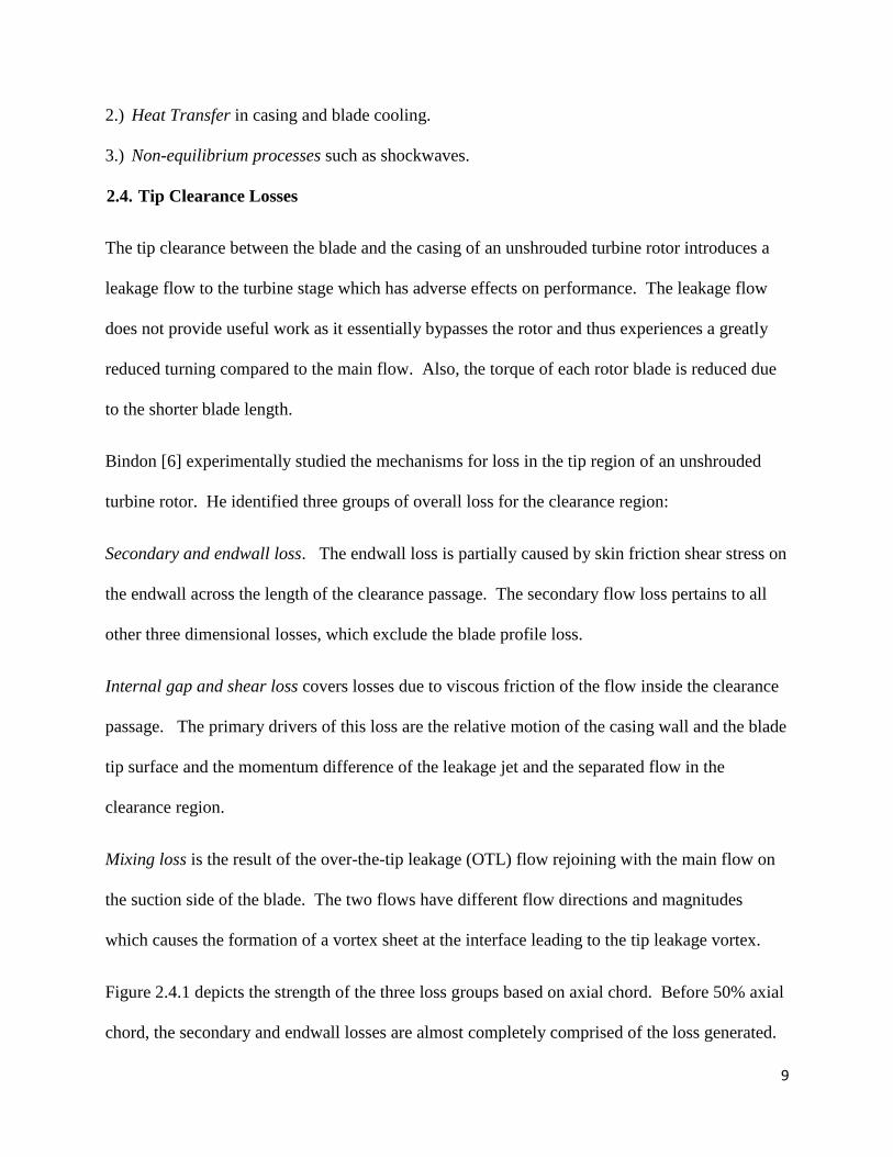
Mixing loss is the result of the over-the-tip leakage (OTL) flow rejoining with the main flow on

the suction side of the blade. The two flows have different flow directions and magnitudes

which causes the formation of a vortex sheet at the interface leading to the tip leakage vortex.

Figure 2.4.1 depicts the strength of the three loss groups based on axial chord. Before 50% axial

chord, the secondary and endwall losses are almost completely comprised of the loss generated.

10

Internal gap and shear losses become significant after 50% axial chord. Mixing losses do not

become prominent until 70% axial chord. The mixing loss also does not terminate at the trailing

edge. It continues downstream and affects subsequent blade rows.

The goal of modern gas turbine engines is to operate as near to adiabatic flame temperature as

possible which increases cycle efficiency and turbine specific work. Since current alloys cannot

sustain these high temperatures, creative cooling techniques have been employed to achieve the

necessary blade service life. One of the crucial regions in high pressure turbines (HPT) is the

Figure 2.4.1 Endwall loss development for unshrouded turbine rotor[6]

11

blade tip region. These areas experience high thermal loading and are difficult to cool. For

unshrouded rotor blades, optimizing the aerodynamic losses from the over-the-tip leakage (OTL)

flows is also crucial. The losses from the OTL flow account for one third of the overall stage

losses in a gas turbine [17].

The issue with the tip leakage vortex is that it not only lessens the efficiency of the rotor blade

row but the vortices travel downstream and generate more efficiency loss on subsequent blade

rows. Harvey [18] showed that once the tip leakage vortex forms, the OTL can provide no

benefit to the turbine stage. However, Blanco [19] used the mixing from the OTL to enhance the

boundary layer of the turbine casing which allows for a higher diffuser angle before stalling

occurs. To minimize the OTL losses, controlling the tip flow and reducing the strength of the tip

vortex have been the primary goal of current research.

Over the last few decades there have been many studies conducted to reduce the losses generated

from the over-the-tip flow. Farokhi [20] presents a discharge coefficient that is proportional to

the tip leakage flow losses. The loss also varies directly with the velocity distribution of the

blade or in other words the blade loading.

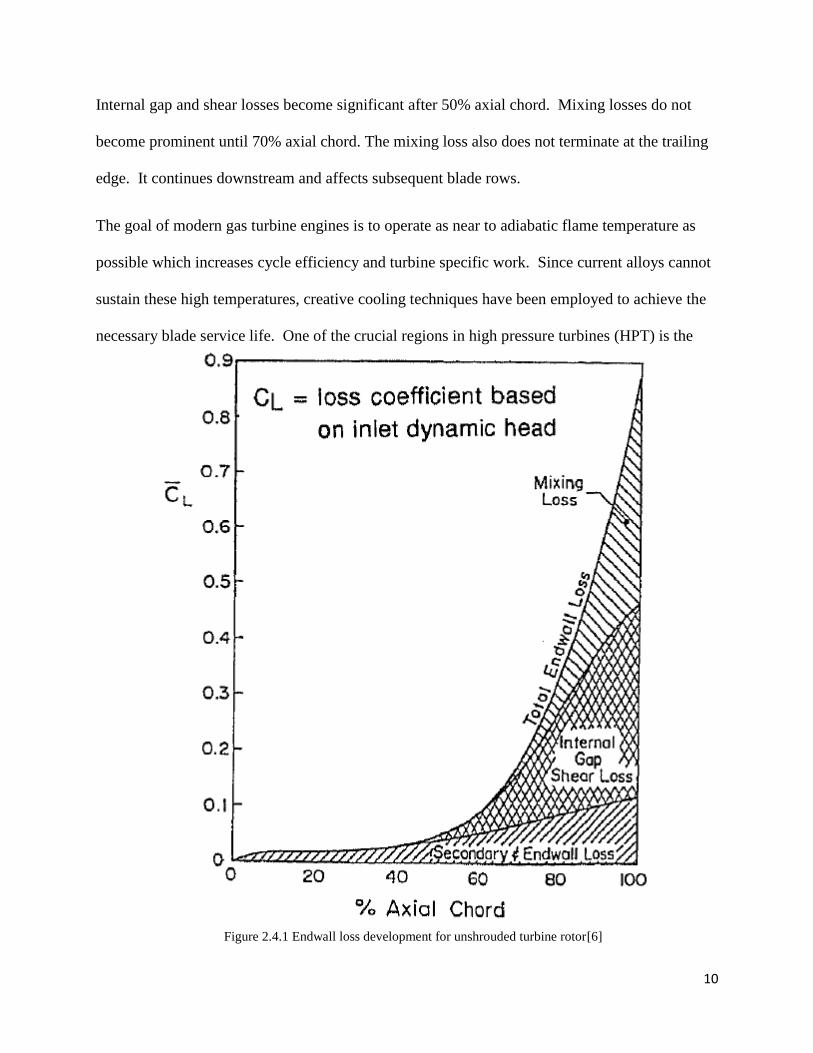
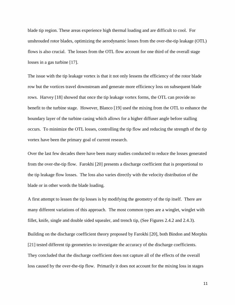
A first attempt to lessen the tip losses is by modifying the geometry of the tip itself. There are

many different variations of this approach. The most common types are a winglet, winglet with

fillet, knife, single and double sided squealer, and trench tip, (See Figures 2.4.2 and 2.4.3).

Building on the discharge coefficient theory proposed by Farokhi [20], both Bindon and Morphis

[21] tested different tip geometries to investigate the accuracy of the discharge coefficients.

They concluded that the discharge coefficient does not capture all of the effects of the overall

loss caused by the over-the-tip flow. Primarily it does not account for the mixing loss in stages

12

downstream of the rotor. Kaiser and Bindon [22] tested different tip geometries in a 1.5 stage

rotating rig where the best performing tip type was a plain smooth tip.

Controlling the tip clearance of the rotor is a popular approach for improving efficiency. There

are two general classes of tip clearance control, active and passive clearance control. An actively

controlled system is able to adjust the clearance for multiple operating points while a passive

control system typically only has one operating point. Lattime and Steinetz [23] compiled an

overview of the active and passive control systems in this field.

Active Thermal Clearance Control utilizes compressor bleed air to heat or cool the rotor casing

segments. This is a slow process which limits the range of clearance control.

Figure 2.4.2 Common turbine rotor tip configurations [7]

Figure 2.4.3 Discharge Coefficient of common turbine rotor tips versus flat tip [7]

13

Active Mechanical Clearance Control as the name suggests uses linkages and actuators to change

the tip clearance by radially moving the rotor casing [24]. The problems this strategy incurs is

lack of suitable actuators and sensors for the high temperature side of the turbine.

Active Pneumatic Clearance Control use either internal or external generated pressure to load

deflectable shroud segments or to fill bellow system to vary the tip clearance. These types of

systems are susceptible to high cycle fatigue (HCF) and are quite sensitive to any pressure

imbalance.

Passive Thermal Clearance Control only use engine temperatures and material properties to

change the tip clearance by matching the expansion and shrinking of the blades [25]. This

system is accurate and reliable but can only be optimized for one operating point, typically

takeoff.

Passive Pneumatic Clearance Controls are similar to the active version but also include systems

that discharge cooling air into the core flow. This second type of control is driven by the

hydrodynamic effects of the cooling and the core flows. Past investigations include Huber [26]

who placed a slot near the pressure side of the rotor tip to inject air that opposed the over-the-tip

flow. Dey [27] and Rao [28] examined the effects of different jet impingement positions on the

blade tip and blowing ratios. The radial position of the leakage vortex and the strength of the

vortex were found to be influenced by these jets. Behr presented a case with circular jets inclined

against the motion of the tip flow [13]. He found that using 1% injection mass flow reduced the

TKE 25% and using 0.7% injection at 30% axial chord produced the optimal turbine efficiency

gain of 0.55%.

14

From the difficulty present with active systems in the harsh high pressure turbine (HPT)

environment, one can conclude that passive systems with no moving parts are the future of tip

clearance control. A robust system with incorporated cooling is highly desirable. The current

research will address the concept of using fluidic oscillators to inject rotor cooling air into the tip

clearance region thereby mitigating the tip leakage flow.

2.5. For Active Flow Control

One of the most attractive features of fluidic oscillators is their ability to produce periodic

oscillating jets without the need for moving mechanical parts. The operation of fluidic

oscillators is fundamentally based upon the Coanda effect.

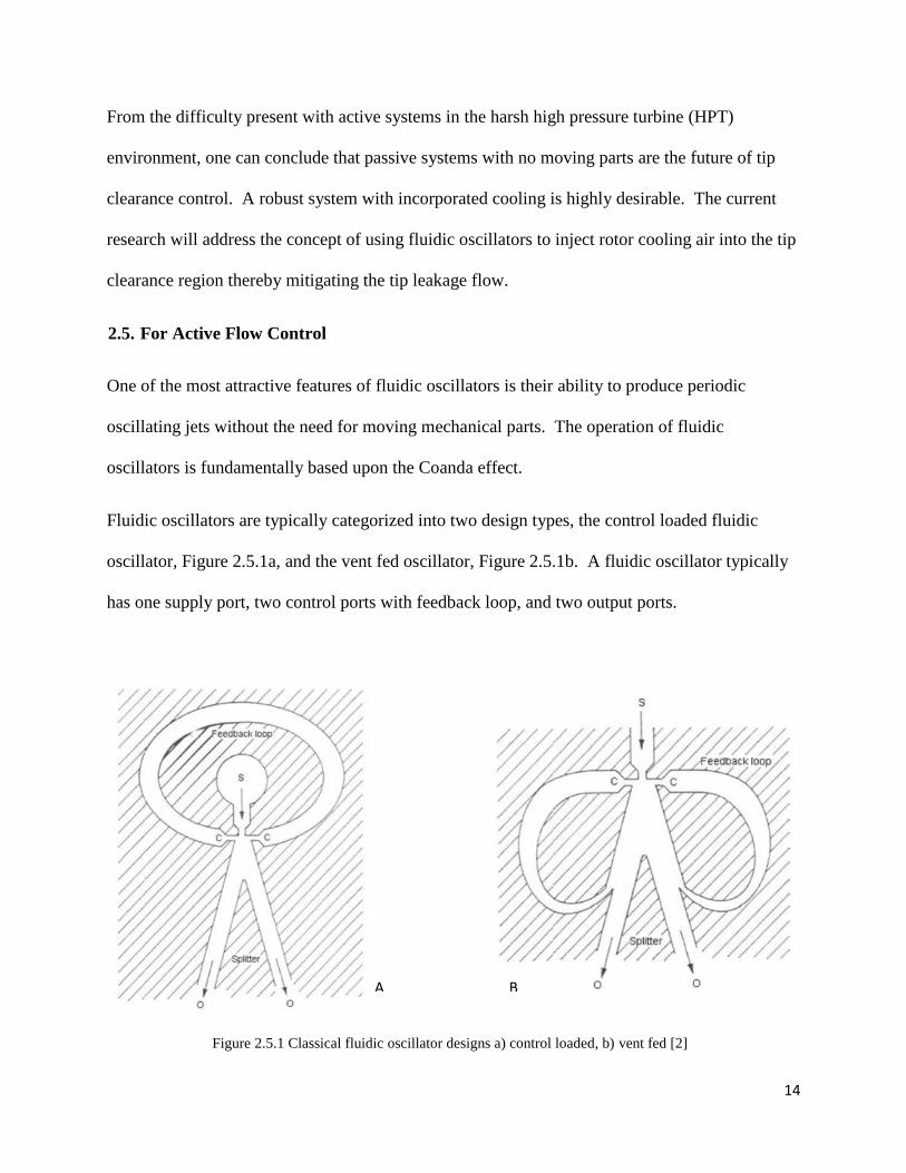
Fluidic oscillators are typically categorized into two design types, the control loaded fluidic

oscillator, Figure 2.5.1a, and the vent fed oscillator, Figure 2.5.1b. A fluidic oscillator typically

has one supply port, two control ports with feedback loop, and two output ports.

Figure 2.5.1 Classical fluidic oscillator designs a) control loaded, b) vent fed [2]

A B

15

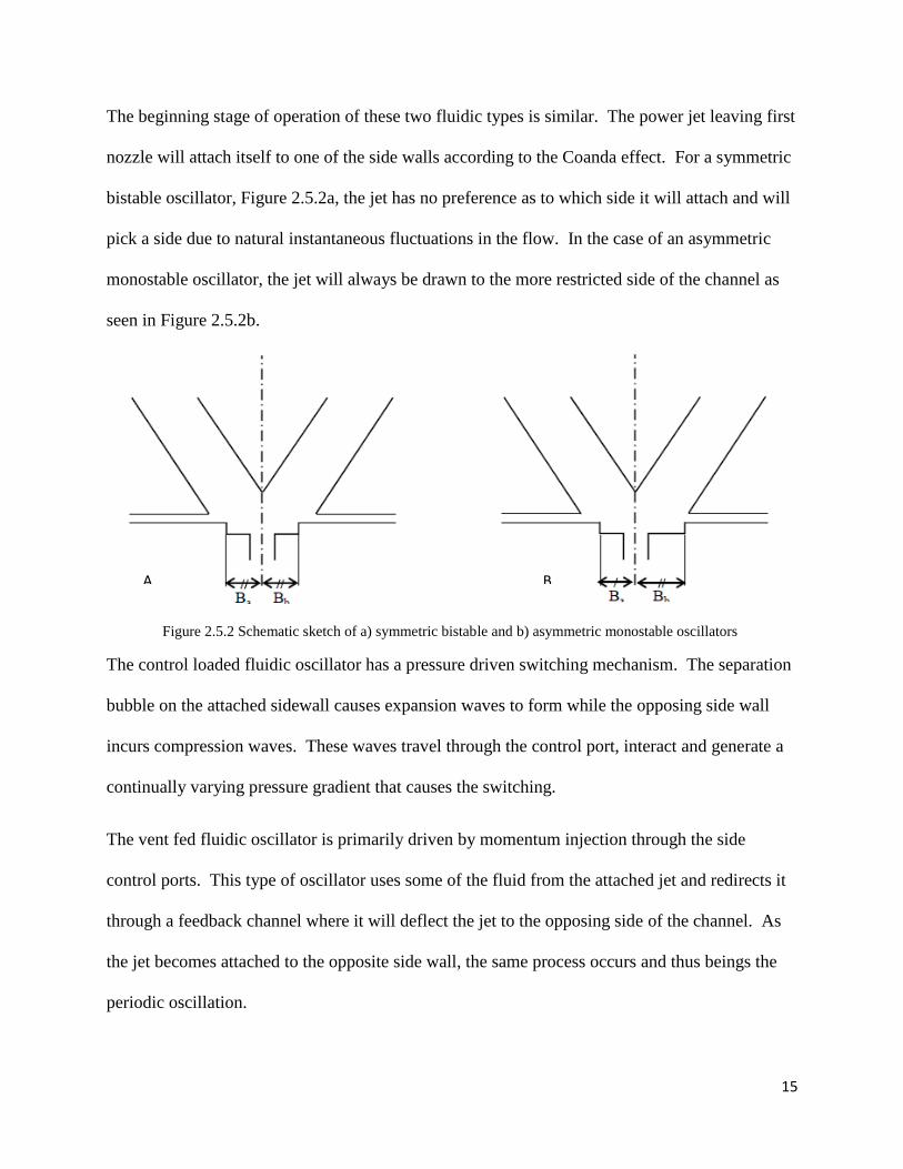
The beginning stage of operation of these two fluidic types is similar. The power jet leaving first

nozzle will attach itself to one of the side walls according to the Coanda effect. For a symmetric

bistable oscillator, Figure 2.5.2a, the jet has no preference as to which side it will attach and will

pick a side due to natural instantaneous fluctuations in the flow. In the case of an asymmetric

monostable oscillator, the jet will always be drawn to the more restricted side of the channel as

seen in Figure 2.5.2b.

The control loaded fluidic oscillator has a pressure driven switching mechanism. The separation

bubble on the attached sidewall causes expansion waves to form while the opposing side wall

incurs compression waves. These waves travel through the control port, interact and generate a

continually varying pressure gradient that causes the switching.

The vent fed fluidic oscillator is primarily driven by momentum injection through the side

control ports. This type of oscillator uses some of the fluid from the attached jet and redirects it

through a feedback channel where it will deflect the jet to the opposing side of the channel. As

the jet becomes attached to the opposite side wall, the same process occurs and thus beings the

periodic oscillation.

Figure 2.5.2 Schematic sketch of a) symmetric bistable and b) asymmetric monostable oscillators

A B

16

The frequency of oscillation for both types of oscillators is determined by the geometry of the

oscillator as well as the aerothermal properties of the fluid in the feedback channels.

Since these oscillators are able to produce pulsating jets without the need for moving mechanical

parts, they offer many advantages over conventional pulsed jet actuators. Main advantages

include greater robustness for environmental and mechanical conditions, i.e. no fatigue failure of

moving parts. Also the simplicity of the device allows for smaller space requirements and

maintenance work. This will result in lower lifetime cost of fluidic systems.

Over the past decade, most of the research into fluidic systems has been for flow control

applications. This research includes investigating the fundamental characteristics of different

fluidic oscillator designs, [29], [30], [31], and validation of such devises for internal and external

flow applications, [32], [33], [34]. There have also been studies on the viability of combining

existing flow control actuators such as piezoelectric transducer and plasma actuator with a fluidic

oscillator to gain complete control of the jet switching independent of the natural mechanisms,

[35], [36].

3. Computational Setup

3.1. STAR-CCM+

STAR-CCM+ is the comprehensive engineering physics simulator developed by CD-Adapco. It

includes a CAD modeling and surface repair, automatic meshing technology, physics and

turbulence modeling as well as post-processing and CAE Integration. It is also able to

seamlessly combine with popular CAD environments such as NX and Pro/E. STAR-CCM+ is a

robust commercial simulator which is capable of simulating segregated, coupled, and finite

volume solid stress, steady and unsteady flows. It uses many different turbulence, compressible,

17

and heat transfer models as well as multiphase and combustion and chemical reaction

simulations.

3.2. Polyhedral vs. Tetrahedral Mesh

STAR-CCM+ includes automatic meshers for unstructured tetrahedral and polyhedral

meshes. Any volume can be discretized using tetrahedrons or polyhedrons; however, using

polyhedral elements for meshing provides significant benefits over using a tetrahedral mesh.

Tetrahedron are the simplest volume element to define. They have easy to calculate face

and volume centroid locations making them well suited for automatic mesh generation.

Tetrahedron do not retain accuracy when they are greatly skewed in areas such as boundary

layers, narrow channels, and tip clearance region of rotor blades. To retain reasonable accuracy,

the automatic mesher will subdivide the highly skewed elements until the skewness criterion is

met which greatly increases the total number elements defining the volume.

Tetrahedron elements, Figure 3.2.1b, only have 4 surrounding neighbors with which to

communicate. Gradients become difficult calculate since the neighboring nodes are all nearly

planar. Another problem occurs with elements near boundaries, edges, and corners. There may

only be one or two neighbor elements on the same surface causing numerical issues and reduced

accuracy. To achieve an accurate solution and good convergence, tetrahedral meshes require

specialized discretization techniques and a great many elements. These requirements are not

ideal solution as the special techniques require complex coding and the large element count

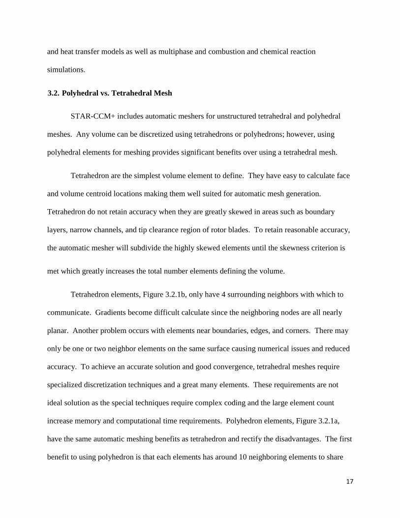
increase memory and computational time requirements. Polyhedron elements, Figure 3.2.1a,

have the same automatic meshing benefits as tetrahedron and rectify the disadvantages. The first

benefit to using polyhedron is that each elements has around 10 neighboring elements to share

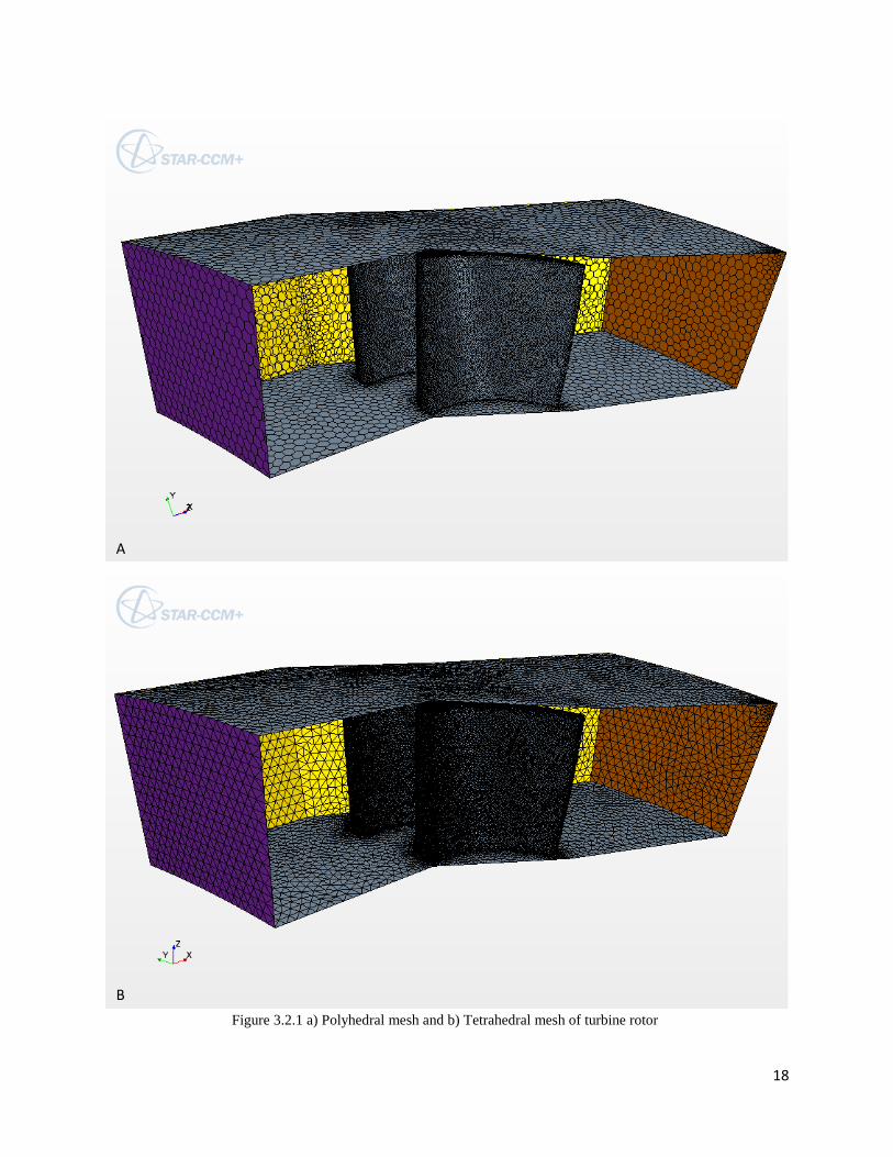
18

Figure 3.2.1 a) Polyhedral mesh and b) Tetrahedral mesh of turbine rotor

A

B

19

information. So gradients can be much better approximated. Along edges and corners there are

more neighbors leading to better local flow distribution. The higher node count per element

causes higher storage and computation requirements but the increased accuracy per element

actually reduces overall computation time and element count. Polyhedral elements are much

more robust than tetrahedron. They can be automatically stretched, joined, split, or modified by

adding points, edges and faces without losing significant accuracy. Locations that would require

special methods to solve with a tetrahedron mesh such as sliding grid, periodic boundary, and

local mesh refinement are no longer a problem for a polyhedral mesh since the element is so

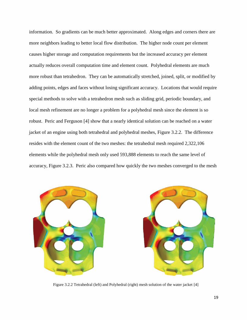
robust. Peric and Ferguson [4] show that a nearly identical solution can be reached on a water

jacket of an engine using both tetrahedral and polyhedral meshes, Figure 3.2.2. The difference

resides with the element count of the two meshes: the tetrahedral mesh required 2,322,106

elements while the polyhedral mesh only used 593,888 elements to reach the same level of

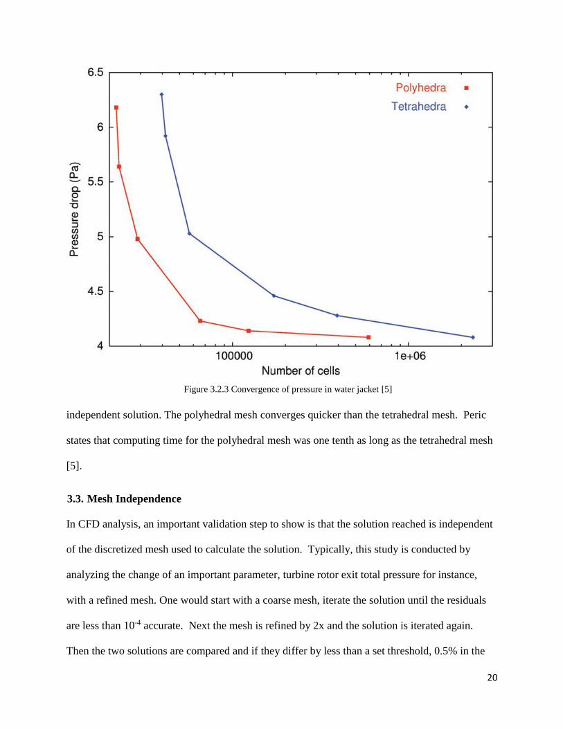
accuracy, Figure 3.2.3. Peric also compared how quickly the two meshes converged to the mesh

Figure 3.2.2 Tetrahedral (left) and Polyhedral (right) mesh solution of the water jacket [4]

20

independent solution. The polyhedral mesh converges quicker than the tetrahedral mesh. Peric

states that computing time for the polyhedral mesh was one tenth as long as the tetrahedral mesh

[5].

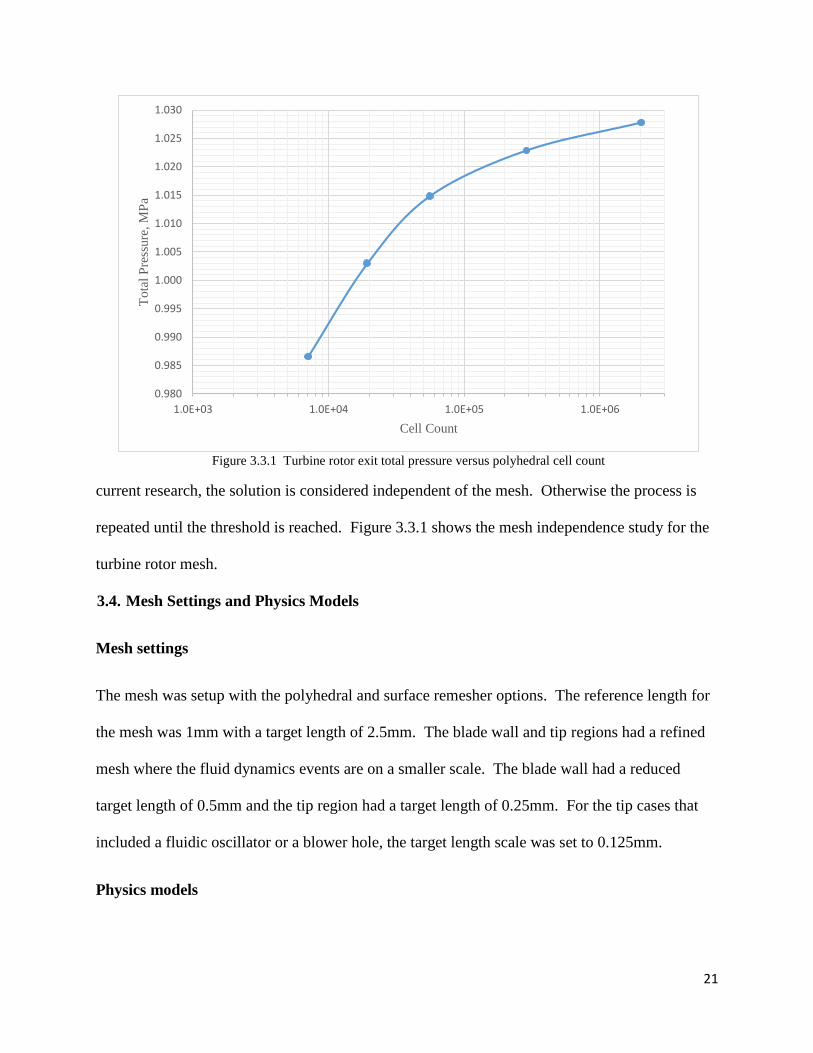
3.3. Mesh Independence

In CFD analysis, an important validation step to show is that the solution reached is independent

of the discretized mesh used to calculate the solution. Typically, this study is conducted by

analyzing the change of an important parameter, turbine rotor exit total pressure for instance,

with a refined mesh. One would start with a coarse mesh, iterate the solution until the residuals

are less than 10-4 accurate. Next the mesh is refined by 2x and the solution is iterated again.

Then the two solutions are compared and if they differ by less than a set threshold, 0.5% in the

Figure 3.2.3 Convergence of pressure in water jacket [5]

21

current research, the solution is considered independent of the mesh. Otherwise the process is

repeated until the threshold is reached. Figure 3.3.1 shows the mesh independence study for the

turbine rotor mesh.

3.4. Mesh Settings and Physics Models

Mesh settings

The mesh was setup with the polyhedral and surface remesher options. The reference length for

the mesh was 1mm with a target length of 2.5mm. The blade wall and tip regions had a refined

mesh where the fluid dynamics events are on a smaller scale. The blade wall had a reduced

target length of 0.5mm and the tip region had a target length of 0.25mm. For the tip cases that

included a fluidic oscillator or a blower hole, the target length scale was set to 0.125mm.

Physics models

0.980

0.985

0.990

0.995

1.000

1.005

1.010

1.015

1.020

1.025

1.030

1.0E+03 1.0E+04 1.0E+05 1.0E+06

To

tal

Pre

ssure

, M

Pa

Cell Count

Figure 3.3.1 Turbine rotor exit total pressure versus polyhedral cell count

22

The physics models chosen to simulate the turbine tip clearance problem include: coupled flow,

gas-hot air mediums, ideal gas law, implicit unsteady, k-ε turbulence model, and 3-D flow field.

The coupled flow model is a more robust and accurate model for compressible flows than a

segregated model. Also the number of iterations required to solve a flow problem with the

coupled model is independent of mesh size unlike the segregated model which increases with

mesh size. The medium selected for the problem was hot air properties selected, 𝛾 = 1.33, 𝑐𝑝 =

1156 𝐽/(𝑘𝑔𝐾). The ideal gas model was used to allow for compressible flow calculations. The

fact that the turbine has a moving rotor blade row requires adaption of an unsteady model. The

implicit unsteady model was chosen over the explicit model for more control over the time step

size, iteration per step, etc. Also, all the flow features were in the subsonic regime. The k-ε

turbulence model was used for its robustness and relative ease with decent accuracy in solving

the two equation model. The turbine rotor is moving piece of machinery. To simulate this

effect, the entire volume mesh is rotated about the z-axis at a rate of 5000 rpm. The time step

was chosen to be 2.08E-5 seconds to allow for about one-half degree of rotation per time step.

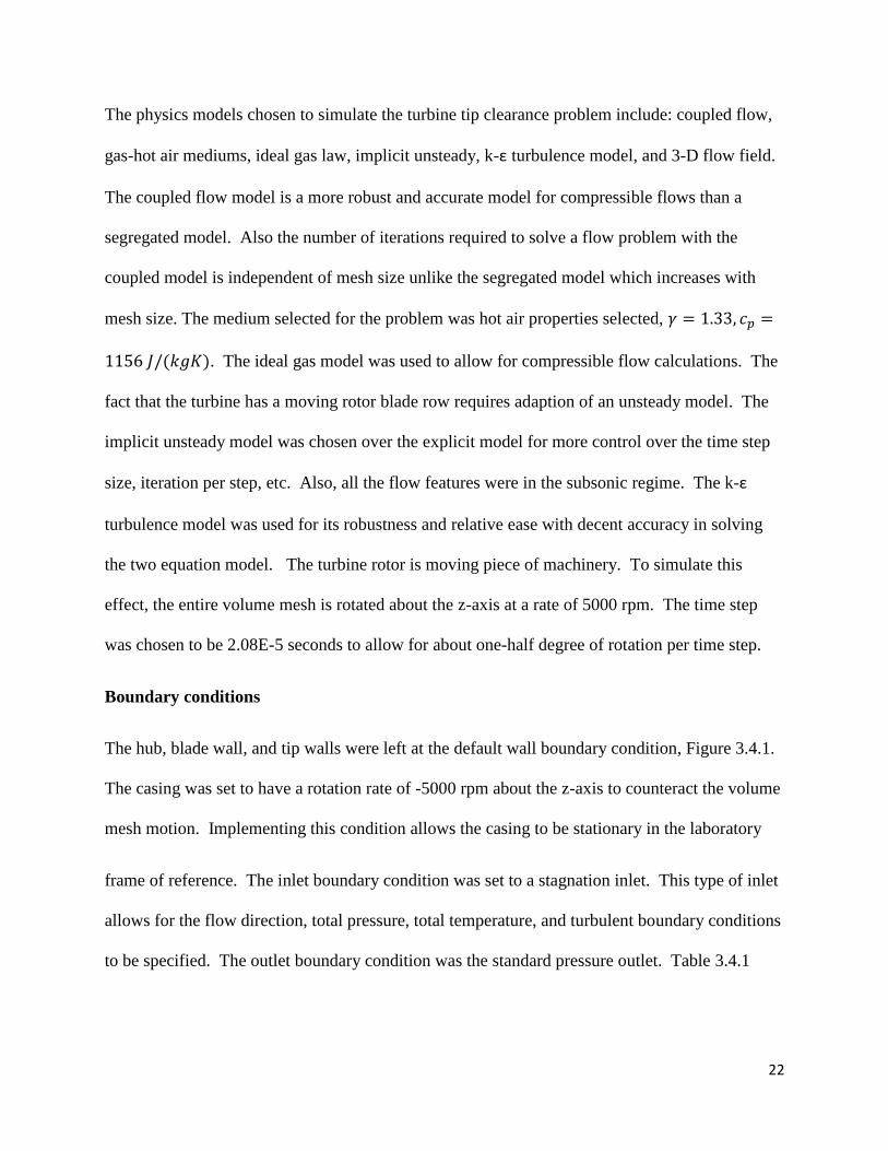
Boundary conditions

The hub, blade wall, and tip walls were left at the default wall boundary condition, Figure 3.4.1.

The casing was set to have a rotation rate of -5000 rpm about the z-axis to counteract the volume

mesh motion. Implementing this condition allows the casing to be stationary in the laboratory

frame of reference. The inlet boundary condition was set to a stagnation inlet. This type of inlet

allows for the flow direction, total pressure, total temperature, and turbulent boundary conditions

to be specified. The outlet boundary condition was the standard pressure outlet. Table 3.4.1

23

shows the values of the inlet and outlet boundary conditions. The side regions were set to be

rotationally periodic about the z-axis.

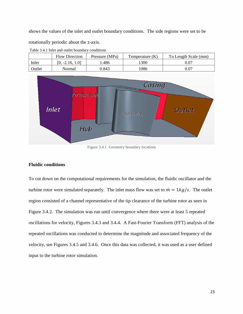
Fluidic conditions

To cut down on the computational requirements for the simulation, the fluidic oscillator and the

turbine rotor were simulated separately. The inlet mass flow was set to �̇� = 1𝑘𝑔/𝑠. The outlet

region consisted of a channel representative of the tip clearance of the turbine rotor as seen in

Figure 3.4.2. The simulation was run until convergence where there were at least 5 repeated

oscillations for velocity, Figures 3.4.3 and 3.4.4. A Fast-Fourier Transform (FFT) analysis of the

repeated oscillations was conducted to determine the magnitude and associated frequency of the

velocity, see Figures 3.4.5 and 3.4.6. Once this data was collected, it was used as a user defined

input to the turbine rotor simulation.

Flow Direction Pressure (MPa) Temperature (K) Tu Length Scale (mm)

Inlet [0, -2.16, 1.0] 1.486 1300 0.07

Outlet Normal 0.843 1086 0.07

Figure 3.4.1 Geometry boundary locations

Table 3.4.1 Inlet and outlet boundary conditions

24

Fluidic Oscillator

Tip Clearance Channel

Figure 3.4.2 Fluidic oscillator CAD geometry

Figure 3.4.3 Convergence of x velocity at fluidic exit

25

Figure 3.4.4 Convergence of y velocity at fluidic exit

Figure 3.4.5 FFT of x velocity at fluidic exit

26

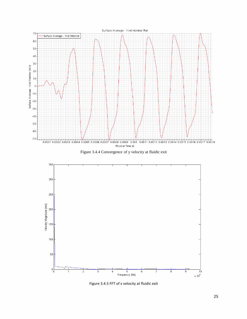
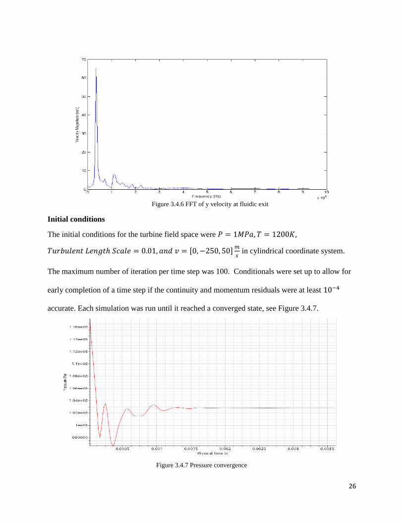
Initial conditions

The initial conditions for the turbine field space were 𝑃 = 1𝑀𝑃𝑎, 𝑇 = 1200𝐾,

𝑇𝑢𝑟𝑏𝑢𝑙𝑒𝑛𝑡 𝐿𝑒𝑛𝑔𝑡ℎ 𝑆𝑐𝑎𝑙𝑒 = 0.01, 𝑎𝑛𝑑 𝑣 = [0, −250, 50]𝑚

𝑠 in cylindrical coordinate system.

The maximum number of iteration per time step was 100. Conditionals were set up to allow for

early completion of a time step if the continuity and momentum residuals were at least 10−4

accurate. Each simulation was run until it reached a converged state, see Figure 3.4.7.

Figure 3.4.6 FFT of y velocity at fluidic exit

Figure 3.4.7 Pressure convergence

27

4. Results

4.1. Mass Flow Injection

All of the tip configurations investigated exhibit the following effects. They may be more or less

pronounced depending upon the individual configuration.

4.1.1. Tip Leakage Vortex

Reduction of turbulence intensity

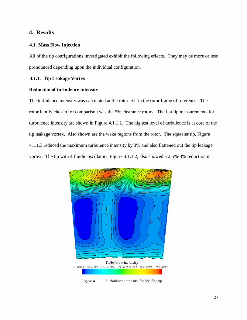
The turbulence intensity was calculated at the rotor exit in the rotor frame of reference. The

rotor family chosen for comparison was the 5% clearance rotors. The flat tip measurements for

turbulence intensity are shown in Figure 4.1.1.1. The highest level of turbulence is at core of the

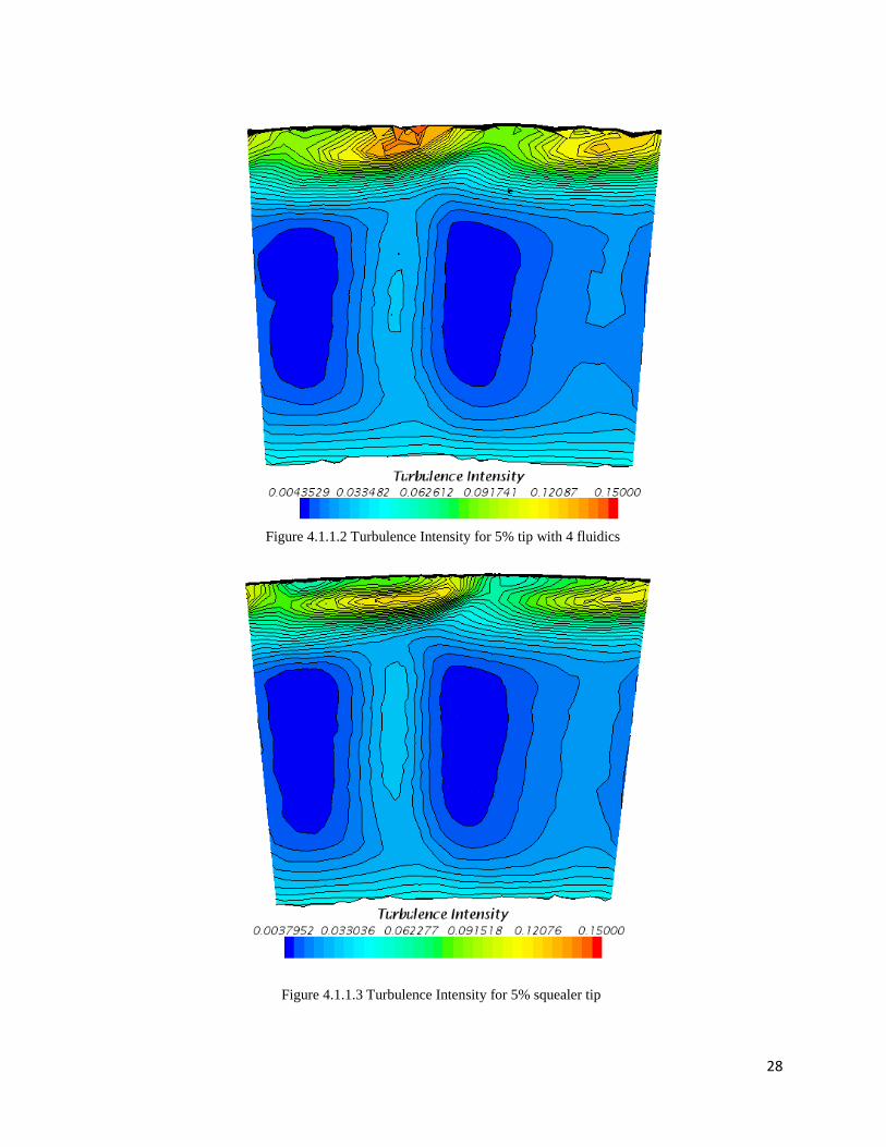
tip leakage vortex. Also shown are the wake regions from the rotor. The squealer tip, Figure

4.1.1.3 reduced the maximum turbulence intensity by 3% and also flattened out the tip leakage

vortex. The tip with 4 fluidic oscillators, Figure 4.1.1.2, also showed a 2.5%-3% reduction in

Figure 4.1.1.1 Turbulence intensity for 5% flat tip

28

Figure 4.1.1.2 Turbulence Intensity for 5% tip with 4 fluidics

Figure 4.1.1.3 Turbulence Intensity for 5% squealer tip

29

turbulence intensity for the tip leakage vortex. The reduction in core intensity manifests in a

reduction of the entire tip region intensity.

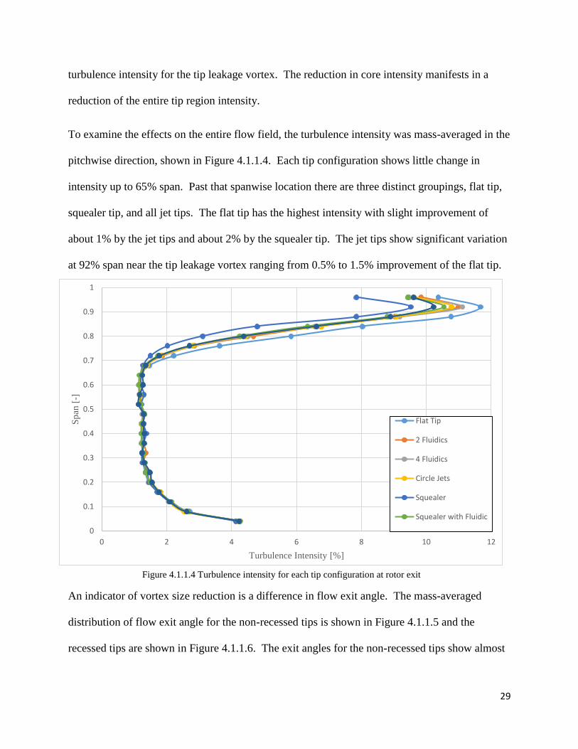
To examine the effects on the entire flow field, the turbulence intensity was mass-averaged in the

pitchwise direction, shown in Figure 4.1.1.4. Each tip configuration shows little change in

intensity up to 65% span. Past that spanwise location there are three distinct groupings, flat tip,

squealer tip, and all jet tips. The flat tip has the highest intensity with slight improvement of

about 1% by the jet tips and about 2% by the squealer tip. The jet tips show significant variation

at 92% span near the tip leakage vortex ranging from 0.5% to 1.5% improvement of the flat tip.

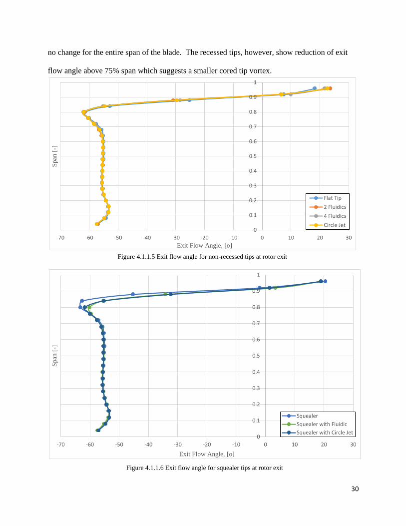
An indicator of vortex size reduction is a difference in flow exit angle. The mass-averaged

distribution of flow exit angle for the non-recessed tips is shown in Figure 4.1.1.5 and the

recessed tips are shown in Figure 4.1.1.6. The exit angles for the non-recessed tips show almost

0

0.1

0.2

0.3

0.4

0.5

0.6

0.7

0.8

0.9

1

0 2 4 6 8 10 12

Sp

an [

-]

Turbulence Intensity [%]

Flat Tip

2 Fluidics

4 Fluidics

Circle Jets

Squealer

Squealer with Fluidic

Figure 4.1.1.4 Turbulence intensity for each tip configuration at rotor exit

30

no change for the entire span of the blade. The recessed tips, however, show reduction of exit

flow angle above 75% span which suggests a smaller cored tip vortex.

0

0.1

0.2

0.3

0.4

0.5

0.6

0.7

0.8

0.9

1

-70 -60 -50 -40 -30 -20 -10 0 10 20 30

Sp

an [

-]

Exit Flow Angle, [o]

Flat Tip

2 Fluidics

4 Fluidics

Circle Jet

Figure 4.1.1.5 Exit flow angle for non-recessed tips at rotor exit

0

0.1

0.2

0.3

0.4

0.5

0.6

0.7

0.8

0.9

1

-70 -60 -50 -40 -30 -20 -10 0 10 20 30

Sp

an [

-]

Exit Flow Angle, [o]

Squealer

Squealer with Fluidic

Squealer with Circle Jet

Figure 4.1.1.6 Exit flow angle for squealer tips at rotor exit

31

The pressure coefficient corrected for compressibility effects and applied to total pressure was

calculated using Laitone’s rule,

𝐶𝑝 =

𝐶𝑝0

√1 − 𝑀∞2 +

𝑀∞2

1 + √1 − 𝑀∞2

(𝐶𝑝0

2 )

4.1.1

where 𝐶𝑝0 =2

𝛾𝑀∞2 (

𝑝

𝑝∞− 1) is incompressible pressure coefficient. Up to 75% span, the total

pressure coefficient is negative since the reference total pressure was set to 1𝑀𝑃𝑎 and this

region has a lower total pressure, Figure 4.1.1.7. In each of the tip configurations, there is a

reduction in total pressure coefficient compared to both the flat tip and squealer tip. This

0

0.1

0.2

0.3

0.4

0.5

0.6

0.7

0.8

0.9

1

-1 -0.5 0 0.5 1 1.5 2 2.5

Sp

an [

-]

Total Pressure Coefficient [-]

Flat Tip

2 Fluidics

4 Fluidics

Circle Jets

Squealer

Squealer with Fluidic

Squealer with Circle Jet

Figure 4.1.1.7 Total pressure coefficient at rotor exit

32

indicates a weaker pressure gradient between the tip leakage flow and the core flow which

ultimately reduces the strength of the tip leakage vortex.

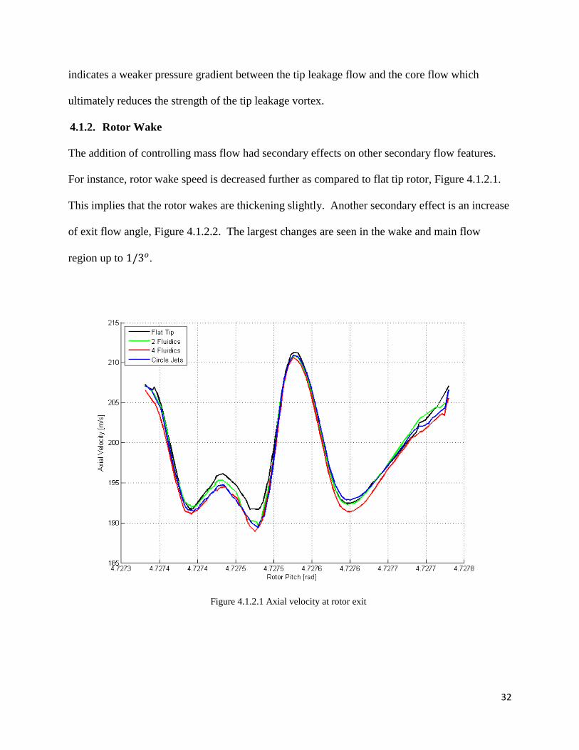
4.1.2. Rotor Wake

The addition of controlling mass flow had secondary effects on other secondary flow features.

For instance, rotor wake speed is decreased further as compared to flat tip rotor, Figure 4.1.2.1.

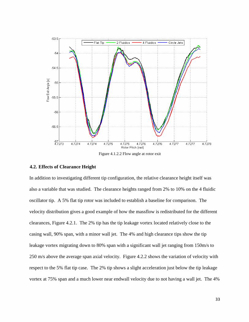
This implies that the rotor wakes are thickening slightly. Another secondary effect is an increase

of exit flow angle, Figure 4.1.2.2. The largest changes are seen in the wake and main flow

region up to 1/3𝑜.

Figure 4.1.2.1 Axial velocity at rotor exit

33

4.2. Effects of Clearance Height

In addition to investigating different tip configuration, the relative clearance height itself was

also a variable that was studied. The clearance heights ranged from 2% to 10% on the 4 fluidic

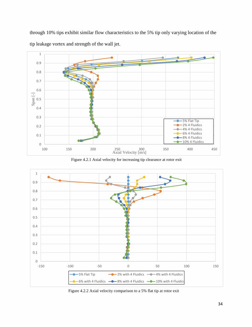
oscillator tip. A 5% flat tip rotor was included to establish a baseline for comparison. The

velocity distribution gives a good example of how the massflow is redistributed for the different

clearances, Figure 4.2.1. The 2% tip has the tip leakage vortex located relatively close to the

casing wall, 90% span, with a minor wall jet. The 4% and high clearance tips show the tip

leakage vortex migrating down to 80% span with a significant wall jet ranging from 150m/s to

250 m/s above the average span axial velocity. Figure 4.2.2 shows the variation of velocity with

respect to the 5% flat tip case. The 2% tip shows a slight acceleration just below the tip leakage

vortex at 75% span and a much lower near endwall velocity due to not having a wall jet. The 4%

Figure 4.1.2.2 Flow angle at rotor exit

34

through 10% tips exhibit similar flow characteristics to the 5% tip only varying location of the

tip leakage vortex and strength of the wall jet.

0

0.1

0.2

0.3

0.4

0.5

0.6

0.7

0.8

0.9

1

100 150 200 250 300 350 400 450

Sp

an [

-]

Axial Velocity [m/s]

5% Flat Tip2% 4 Fluidics4% 4 Fluidics6% 4 Fluidics8% 4 Fluidics10% 4 Fluidics

0

0.1

0.2

0.3

0.4

0.5

0.6

0.7

0.8

0.9

1

-150 -100 -50 0 50 100 150

5% Flat Tip 2% with 4 Fluidics 4% with 4 Fluidics

6% with 4 Fluidics 8% with 4 Fluidics 10% with 4 Fluidics

Figure 4.2.1 Axial velocity for increasing tip clearance at rotor exit

Figure 4.2.2 Axial velocity comparison to a 5% flat tip at rotor exit

35

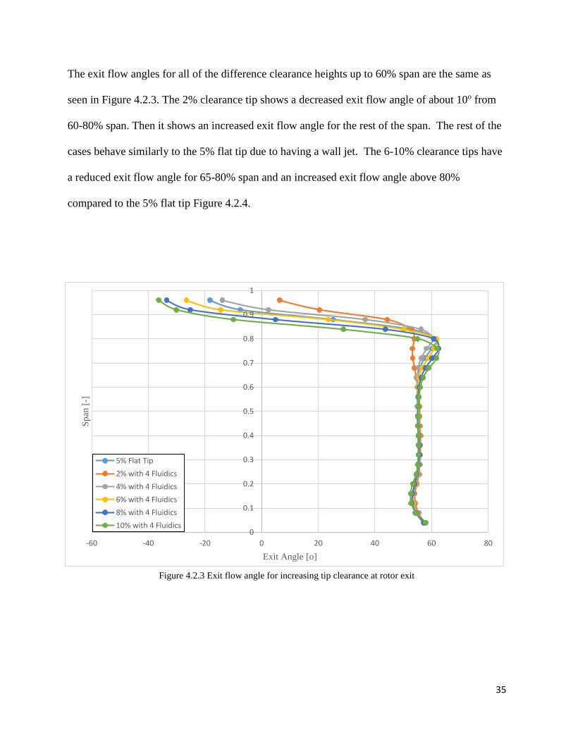
The exit flow angles for all of the difference clearance heights up to 60% span are the same as

seen in Figure 4.2.3. The 2% clearance tip shows a decreased exit flow angle of about 10o from

60-80% span. Then it shows an increased exit flow angle for the rest of the span. The rest of the

cases behave similarly to the 5% flat tip due to having a wall jet. The 6-10% clearance tips have

a reduced exit flow angle for 65-80% span and an increased exit flow angle above 80%

compared to the 5% flat tip Figure 4.2.4.

0

0.1

0.2

0.3

0.4

0.5

0.6

0.7

0.8

0.9

1

-60 -40 -20 0 20 40 60 80

Sp

an [

-]

Exit Angle [o]

5% Flat Tip

2% with 4 Fluidics

4% with 4 Fluidics

6% with 4 Fluidics

8% with 4 Fluidics

10% with 4 Fluidics

Figure 4.2.3 Exit flow angle for increasing tip clearance at rotor exit

36

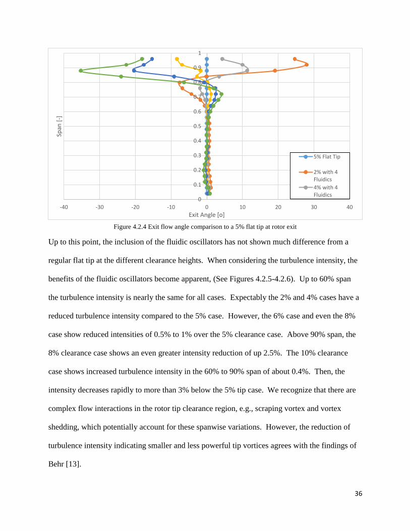
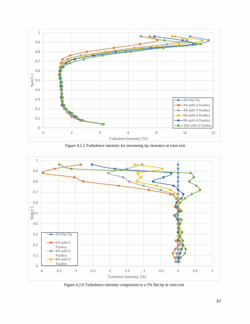
Up to this point, the inclusion of the fluidic oscillators has not shown much difference from a

regular flat tip at the different clearance heights. When considering the turbulence intensity, the

benefits of the fluidic oscillators become apparent, (See Figures 4.2.5-4.2.6). Up to 60% span

the turbulence intensity is nearly the same for all cases. Expectably the 2% and 4% cases have a

reduced turbulence intensity compared to the 5% case. However, the 6% case and even the 8%

case show reduced intensities of 0.5% to 1% over the 5% clearance case. Above 90% span, the

8% clearance case shows an even greater intensity reduction of up 2.5%. The 10% clearance

case shows increased turbulence intensity in the 60% to 90% span of about 0.4%. Then, the

intensity decreases rapidly to more than 3% below the 5% tip case. We recognize that there are

complex flow interactions in the rotor tip clearance region, e.g., scraping vortex and vortex

shedding, which potentially account for these spanwise variations. However, the reduction of

turbulence intensity indicating smaller and less powerful tip vortices agrees with the findings of

Behr [13].

0

0.1

0.2

0.3

0.4

0.5

0.6

0.7

0.8

0.9

1

-40 -30 -20 -10 0 10 20 30 40

Span

[-]

Exit Angle [o]

5% Flat Tip

2% with 4Fluidics

4% with 4Fluidics

Figure 4.2.4 Exit flow angle comparison to a 5% flat tip at rotor exit

37

0

0.1

0.2

0.3

0.4

0.5

0.6

0.7

0.8

0.9

1

-4 -3.5 -3 -2.5 -2 -1.5 -1 -0.5 0 0.5 1

Sp

an [

-]

Turbulent Intensity [%]

5% Flat Tip

2% with 4Fluidics4% with 4Fluidics6% with 4Fluidics

0

0.1

0.2

0.3

0.4

0.5

0.6

0.7

0.8

0.9

1

0 2 4 6 8 10 12

Sp

an [

-]

Turbulent Intensity [%]

5% Flat Tip

2% with 4 Fluidics

4% with 4 Fluidics

6% with 4 Fluidics

8% with 4 Fluidics

10% with 4 Fluidics

Figure 4.2.5 Turbulence intensity for increasing tip clearance at rotor exit

Figure 4.2.6 Turbulence intensity comparison to a 5% flat tip at rotor exit

38

4.3. Turbine Rotor Efficiency

The rotor aerodynamic efficiency is defined as the ratio of the real and isentropic total enthalpy

𝜂 =

Δ�̇�

Δ�̇�𝑖𝑠

𝑤ℎ𝑒𝑟𝑒 Δ�̇� = �̇�Δℎ𝑡 (4.3.1)

In this experiment, the injected mass flow was less than 1% of the inlet mass flow. The

assumption was made that �̇�𝑖𝑛 ≅ �̇�𝑜𝑢𝑡. Thus the efficiency equation with some manipulation

reduces to

𝜂 =1 −

𝑇𝑡(𝑖+1)

𝑇𝑡𝑖

1 − (𝑝𝑡(𝑖+1)

𝑝𝑡𝑖)

𝛾−1𝛾

(4.3.2)

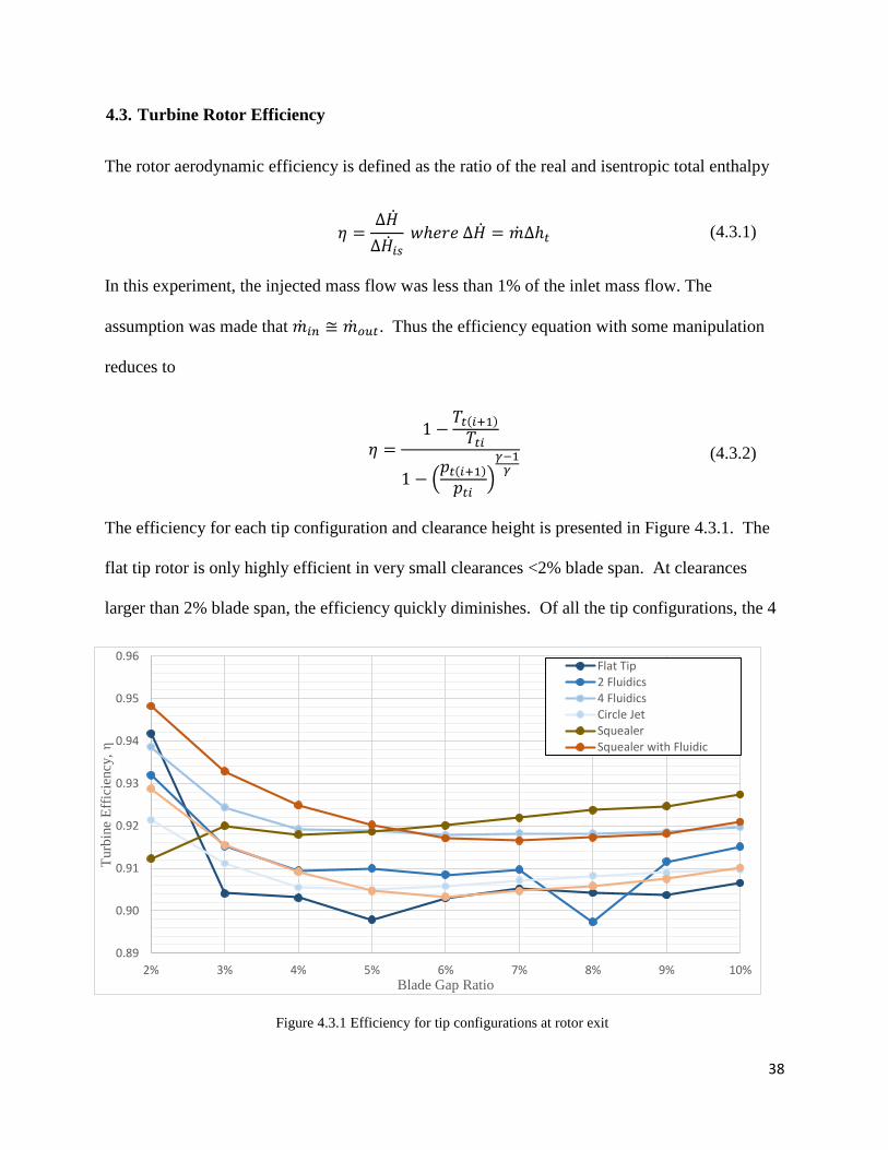
The efficiency for each tip configuration and clearance height is presented in Figure 4.3.1. The

flat tip rotor is only highly efficient in very small clearances <2% blade span. At clearances

larger than 2% blade span, the efficiency quickly diminishes. Of all the tip configurations, the 4

0.89

0.90

0.91

0.92

0.93

0.94

0.95

0.96

2% 3% 4% 5% 6% 7% 8% 9% 10%

Turb

ine

Eff

icie

ncy

, η

Blade Gap Ratio

Flat Tip2 Fluidics4 FluidicsCircle JetSquealerSquealer with Fluidic

Figure 4.3.1 Efficiency for tip configurations at rotor exit

39

fluidics on a flat tip and a recessed tip are the most promising with the highest overall

efficiencies, ~2% better than a flat tip, across all clearances. They are only second to a plain

squealer tip in the 6%-10% clearance heights. Both circle jet configurations show a slight

improvement over a flat tip of 0.5%. The 2 fluidic case is about the same as the circle cases for

clearances of 2% to 4% of blade span and shows an increase of 0.5% for the 5-10% blade span

clearances. The sudden dip in efficiency at 8% clearance height for the 2 fluidic tip is suspected

to be caused by some error in CFD calculation and may not represent the actual efficiency value

at that blade gap ratio.

4.4. Turbine Rotor Power Generation

The efficiency improvement of a particular tip configuration only tells half of the story; the

power generation vs requirement of the new tip must also be considered. Since the turbine and

compressor are connected via the shaft, the power consumed by the compressor is equal to the

power generated by the turbine with mechanical efficiency factor.

𝑃 = 𝜖�̇�𝑐𝑝𝑡(𝑇𝑡(𝑖+1) − 𝑇𝑡𝑖) (4.4.1)

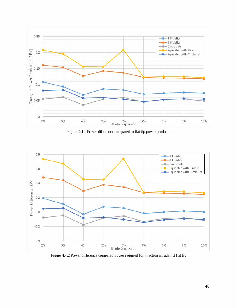
Figure 4.4.1 shows the power increase per orifice for each tip configuration versus a flat tip. All

of the configurations show an increase in turbine production power with the 4 fluidic flat and

squealer tips producing the most. When taking into account the power required to generate this

injected mass flow, Figure 4.4.2 shows the results of this adjustment. The 4 fluidic flat and

squealer tips are producing more power than their requirement at all clearances. The 2 fliudic flat

tip is right on the line for breaking even. The circle jet tips require more power than they

produce in almost all instances.

40

-0.4

-0.2

0

0.2

0.4

0.6

0.8

2% 3% 4% 5% 6% 7% 8% 9% 10%

Po

wer

Dif

fere

nce

[kW

]

Blade Gap Ratio

2 Fluidics4 FluidicsCircle JetsSquealer with FluidicSquealer with Circle Jet

0

0.05

0.1

0.15

0.2

0.25

2% 3% 4% 5% 6% 7% 8% 9% 10%

Chan

ge

in P

ow

er P

rod

uct

ion [

MW

]

Blade Gap Ratio

2 Fluidics4 FluidicsCircle JetsSquealer with FluidicSquealer with Circle Jet

Figure 4.4.1 Power difference compared to flat tip power production

Figure 4.4.2 Power difference compared power required for injection air against flat tip

41

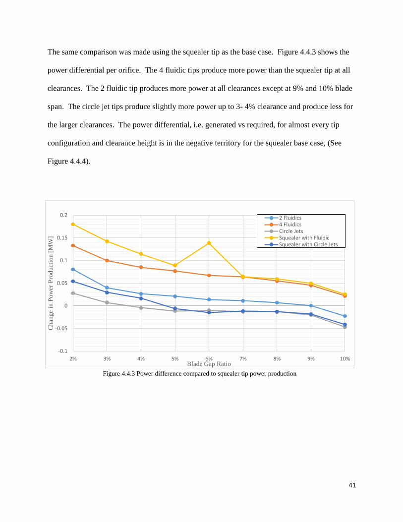
The same comparison was made using the squealer tip as the base case. Figure 4.4.3 shows the

power differential per orifice. The 4 fluidic tips produce more power than the squealer tip at all

clearances. The 2 fluidic tip produces more power at all clearances except at 9% and 10% blade

span. The circle jet tips produce slightly more power up to 3- 4% clearance and produce less for

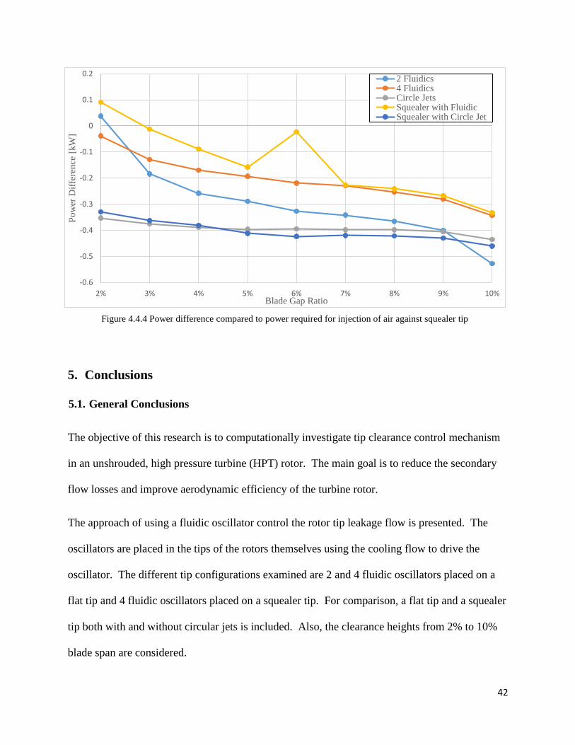
the larger clearances. The power differential, i.e. generated vs required, for almost every tip

configuration and clearance height is in the negative territory for the squealer base case, (See

Figure 4.4.4).

-0.1

-0.05

0

0.05

0.1

0.15

0.2

2% 3% 4% 5% 6% 7% 8% 9% 10%

Chan

ge

in P

ow

er P

rod

uct

ion [

MW

]

Blade Gap Ratio

2 Fluidics4 FluidicsCircle JetsSquealer with FluidicSquealer with Circle Jets

Figure 4.4.3 Power difference compared to squealer tip power production

42

5. Conclusions

5.1. General Conclusions

The objective of this research is to computationally investigate tip clearance control mechanism

in an unshrouded, high pressure turbine (HPT) rotor. The main goal is to reduce the secondary

flow losses and improve aerodynamic efficiency of the turbine rotor.

The approach of using a fluidic oscillator control the rotor tip leakage flow is presented. The

oscillators are placed in the tips of the rotors themselves using the cooling flow to drive the

oscillator. The different tip configurations examined are 2 and 4 fluidic oscillators placed on a

flat tip and 4 fluidic oscillators placed on a squealer tip. For comparison, a flat tip and a squealer

tip both with and without circular jets is included. Also, the clearance heights from 2% to 10%

blade span are considered.

-0.6

-0.5

-0.4

-0.3

-0.2

-0.1

0

0.1

0.2

2% 3% 4% 5% 6% 7% 8% 9% 10%

Po

wer

Dif

fere

nce

[kW

]

Blade Gap Ratio

2 Fluidics4 FluidicsCircle JetsSquealer with FluidicSquealer with Circle Jet

Figure 4.4.4 Power difference compared to power required for injection of air against squealer tip

43

The 4 fluidic oscillator cases show the highest efficiency gain of 2-3% compared to the flat tip

over all clearance heights. They only show slight efficiency gain compared to the squealer tip up

until a clearance of 5% blade span and they show about 1% gain compared to the circle jet tips.

The 4 fluidic oscillator cases produce nearly two times as much power per orifice as the circle jet

cases. The 2 fluidic tip produce 12-40% more power than the circle jet cases. All jet injecting

cases produce more power than the supply air requires except for the circle jet tips. When

compared to the potential power production of a squealer tip, almost every case shows a deficit

for power gained to power required. Only the 2 fluidics on a flat tip and the 4 fluidics on the

squealer tip show a gain at 2% clearance.

5.2. Recommendations For Future Study

The results of this study have shown the possibility that fluidic oscillators can improve turbine

rotor efficiency with a power gain. Not considered in this study was the structural analysis of

rotor blade. Having the fluidic oscillators inside the tip may present thermal and structural

weaknesses to the rotor that deserves further studies. Placing the fluidic oscillator in the casing

presents a good solution to this problem. Once placed in the casing, the oscillator may be

pivoted to angle against the flow whereas in the rotor tip it was locked into a radial position.

Extending the simulation downstream to include subsequent blade rows would provide a better

system view of the benefits of using fluidic oscillators to mitigate tip clearance loss. Lastly,

conducting this study experimentally on a test rig would provide the validation necessary to

move onto the next step of development, which is system-wide integration and performance

testing.

44

6. References

1. Turbostream-Ltd. http://www.turbostream-cfd.com/case-studies/siemens/. 2015. 2. Morris, N.M., An Introduction to Fluid Logic. 1973: McGraw-Hill. 3. a320neo.com, http://www.a320neo.com/pratt-whitney-pw1000g.php. 2010. 4. Peric, M. and S. Ferguson, The Advantage of Polyhedral Meshes. CD-adapco, 2004. 5. Peric, M., Flow Simulation Using Control Volumes of Arbitrary Polyhedral Shape. ERCOFTAC

Bulletin, 2004. 62. 6. Bindon, J.P., The measurement and Formation of Tip Clearance Loss. ASME Journal of

Turbomachinery, 1989. 111: p. 257-263. 7. Booth, T.C., P.R. Dodge, and H.K. Hepworth, Rotor Tip Leakage: Part I-Basic Methodology.

Transactions of ASME, Journal of Engineering for power, 1982. 104: p. 154-161. 8. L.S. Langston, M.L.N., R.M. Hooper, 3-Dimensional Flow within a Turbine Cascade Passage.

Journal of Engineering for Power, 1977. 99(1): p. 21-28. 9. Hawthorne, W.R., Secondary Circulation in Fluid Flow. Proceedings of the Royal Society of

London. Series A, Mathematical and Physical Sciences, 206 (1086): 374-387, 1951. 10. Hawthorne, W.R., Rotational Flow through Cascades. Journal of Mechanics and Applied

Mathematics, 1955. 11. Gregory-Smith, D.G. and C.P. Graves, Secondary Flow Losses in a Turbine Cascade. Viscous

Effects in Turbomachines, 1983. 12. Sieverding, C.H., Recent Progress in the Understanding of Basic Aspects of Secondary Flows in

Turbine Blade Passages. ASME Journal of Turbomachinery, 1985. 107: p. 248-257. 13. Behr, T., Control of Rotor Tip Leakage and Secondary Flow by Casing Air Injection in Unshrouded

Axial Turbines. PhD Diss. ETH Zurich, 2007. 14. Hodson, H.P., Bladerow Interference Effects in Axial Turbomachinery Stages, in VKI Lecture Series

1998-02. 1998: Von Karman Institute for Fluid Dynamics, Belgium. 15. Binder, A., Schroder, T., Hourmouziadis, J., Turbulence Measurements in a Low-Pressure Turbine.

ASME Journal of Turbomachinery, 1989. 111: p. 153-161. 16. Denton, J.D., Loss Mechanisms in Turbomachines. ASME Journal of Turbomachinery, 1993. 115:

p. 621-656. 17. Booth, T.C., Importance of Tip Leakage Flows in Turbine Design. VKI Lecture Series 1985-05,

1985. 18. Harvey, N.W. Aerothermal Implications of Shroudless and Shrouded Blades. in VKI Lecture Series

2004-02. 2004. 19. Blanco, R.R. and S. Farokhi, Performance Analysis of an Axial Exhaust Diffuser Downstream of an

Unshrouded Turbine. paper presented at the 10th International Conference on Advances in Fluid Mechanics, 2014(Coruna, Spain).

20. Farokhi, S., Analysis of Rotor Tip-Clearance Loss in Axial Flow Turbines. AIAA Journal of Propulsion and Power, 1988. 4(5): p. 452-457.

21. Bindon, J.P. and G. Morphis, The Development of Axial Turbine Leakage Loss for Two Profiled Tip Geometries Using Linear Cascade Data. ASME Paper No. 90-GT-152, 1990.

22. Kaiser, I. and J.P. Bindon, The Effect of Tip Clearance on the Development of Loss Behind a Rotor and a Subsequent Nozzle. ASME Paper No. 97-GT-53, 1997.

23. Lattime, S.B. and B.M. Steinetz, High-Pressure-Turbine Clearance Control Systems: Current Practices and Future Directions. AIAA Journal of Propulsion and Power, 2004. 20: p. 302-311.

24. Tseng, W. and A.A. Hauser, Blade TIp Clearance Control Apparatus with Shroud Segment Position Adjustment by Unison Ring Movement. U.S. Patent 5,035,573, 1991.

45

25. Carpenter, K.D., J.D. Wiedemer, and P.A. Smith, Rotor Blade Outer Tip Seal Apparatus. U.S. Patent 5,639,210, 1997.

26. Huber, F.W. and D.J. Dietrich, Clearance Control for the Turbine of a Gas Turbine Engine. ASME Journal of Turbomachinery, 1997. 122: p. 628-633.

27. Dey, D. and C. Camci. Development of Tip Clearance Flow Downstream of a Rotor Blade with Coolant Injection from a Tip Trench. in 8th ISROMAC Conference. 2000. Honolulu, Hawaii.

28. Rao, N.M. and C. Camci, Axial Turbine Tip Desensitization by Injection from a Tip Trench, Part 1: Effect of Injection Mass Flow Rate. ASME paper No. GT2004-53256, 2004.

29. Tesar, V., Hung, C. H., and Zimmerman, W. B., No-Moving-Part Hybrid-Synthetic Jet Actuator. Sensors and Actuators, 2006. A 125: p. 159-169.

30. Yang, J.T., Chen, C. K., Tsai, K. J., Lin, W. Z., and Sheen, H. J., A novel fluidic oscillator incorporating step-shaped attachment walls. Sensors and Actuators, 2007. A. 135: p. 476-483.

31. Furlan, R., et al., Visualization of Internal Liquid Flow Interaction in Meso Planar Structures. Flow Measurements and Instrumentation, 2006. 17: p. 298-302.

32. Culley, D.E., et al., Active Flow Separation Control of a Stator Vane using Surface Injection in a Multistage Compressor Experiment, in ASME Paper GT2003-38863. ASME Turbo Expo. 2003.

33. Raman, G., and Raghu, S., Cavity Resonance Suppression Using Miniature Fluidic Oscillators. AIAA Journal, 2004. 42(12).

34. Cerretelli, C., Wuerz, W., and Gharaibah, E., Unsteady Separation Control on Wind Turbine Blades Using Fluidic Oscillators. AIAA Journal, 2010. 48(7).

35. Gregory, J.W., Ruotolo, J. C., Byerley, A. R., and McLaughlin, T. E.,, Switching Behaviour of a Plasma-Fluidic Actuator, in 45th Aerospace Sciences Meeting & Exhibit, A.P.N. 2007-0785, Editor. 2007: Reno, NV.

36. Gregory, J.W., et al., Variable-Frequency Fluidic Oscillator Driven by a Piezoelectric Bender. AIAA Journal, 2009. 47(11).