tundra landform and vegetation productivity trend maps for

Data Descriptor: Tundra landformand vegetation productivity trendmaps for the Arctic Coastal Plain ofnorthern AlaskaMark J. Lara1,2, Ingmar Nitze3,4, Guido Grosse3,5 & A. David McGuire6

Arctic tundra landscapes are composed of a complex mosaic of patterned ground features, varying in soilmoisture, vegetation composition, and surface hydrology over small spatial scales (10–100m). Theimportance of microtopography and associated geomorphic landforms in influencing ecosystem structureand function is well founded, however, spatial data products describing local to regional scale distribution ofpatterned ground or polygonal tundra geomorphology are largely unavailable. Thus, our understanding oflocal impacts on regional scale processes (e.g., carbon dynamics) may be limited. We produced two keyspatiotemporal datasets spanning the Arctic Coastal Plain of northern Alaska (~60,000 km2) to evaluateclimate-geomorphological controls on arctic tundra productivity change, using (1) a novel 30mclassification of polygonal tundra geomorphology and (2) decadal-trends in surface greenness using theLandsat archive (1999–2014). These datasets can be easily integrated and adapted in an array of local toregional applications such as (1) upscaling plot-level measurements (e.g., carbon/energy fluxes), (2)mapping of soils, vegetation, or permafrost, and/or (3) initializing ecosystem biogeochemistry, hydrology,and/or habitat modeling.

Design Type time series design • observation design

Measurement Type(s) geographic feature • vegetation layer

Technology Type(s) image analysis • computational modeling technique

Factor Type(s) spatiotemporal_interval

Sample Characteristic(s) North Slope Borough • tundra • coastal plain

1Department of Plant Biology, University of Illinois Urbana-Champaign, Urbana, Illinois 61801, USA. 2Institute ofArctic Biology, University of Alaska Fairbanks, Fairbanks, Alaska 99775, USA. 3Alfred Wegener Institute HelmholtzCentre for Polar and Marine Research, Periglacial Research Unit, 14473 Potsdam, Germany. 4Institute ofGeography Science, University of Potsdam, 14476 Potsdam, Germany. 5Institute of Earth and EnvironmentalScience, University of Potsdam, 14476 Potsdam, Germany. 6U.S. Geological Survey, Alaska Cooperative Fish andWildlife Research Unit, University of Alaska Fairbanks, Fairbanks, Alaska 99775, USA. Correspondence andrequests for materials should be addressed to M.J.L. (email: [email protected]).

OPEN

Received: 10 July 2017

Accepted: 7 February 2018

Published: 10 April 2018

www.nature.com/scientificdata

SCIENTIFIC DATA | 5:180058 | DOI: 10.1038/sdata.2018.58 1

mailto:[email protected]

Background & SummaryArctic polygonal tundra landscapes are highly heterogeneous, disproportionately distributed acrossmesotopographic gradients, varying in surficial geology, ground ice content, and soil thermal regimes1,2.The high density of ice wedges present in this low relief landscape facilitates subtle variations (~0.5 m) insurface microtopography, markedly influencing hydrology3,4, biogeochemistry5–10, and vegetationstructure11,12. Fine-scale differences in microtopography have been shown to control a variety of keyecosystem attributes and processes that influence ecosystem function, such as snow distribution anddepth13, surface and subsurface hydrology13,14, vegetation composition2,11,12, carbon dioxide andmethane fluxes5,6,15,16, soil carbon and nitrogen content17–19, and an array of soil characteristics18,20.Despite the prominent control of microtopography and associated geomorphology on ecosystemfunction, land cover data products available to represent landforms across the Pan-Arctic are strikinglylimited21. The relative absence of these key geospatial datasets characterizing permafrost lowlands, mayseverely limit our ability to understand local scale controls on regional to global scale patterns andprocesses21.

Datasets presented here were developed to investigate the potential local to regional controls on pastand future trajectories of arctic tundra vegetation productivity22, inferred from spatiotemporal patterns ofchange in the Normalized Difference Vegetation Index (NDVI). We present two geospatial data products,(1) a 30 m resolution tundra geomorphology map, and (2) a decadal scale NDVI trend map (1999–2014),developed to represent the landform heterogeneity and associated productivity change across the ArcticCoastal Plain (ACP) of northern Alaska (~60,000 km2). We validated the tundra geomorphology mapusing 1000 reference sites, and evaluated the sensor bias used to develop the NDVI trend map. Producedgeospatial datasets will be useful for an array of applications, some of which may include the (1) upscalingof plot-level measurements (e.g., carbon and energy fluxes), (2) mapping of soils, vegetation, orpermafrost, and/or (3) initializing ecosystem biogeochemistry, hydrology, and/or habitat modeling.

MethodsPolygonal tundra geomorphology mappingWe focused this mapping initiative on the Arctic Coastal tundra region of northern Alaska, whichstretches from the western coast along the Chukchi sea to the Beaufort coastal plains at the Alaskan-Canadian border (latitude: 68–71˚ N; longitude: 140–167˚ W). Two ecological landscape units (~60,000km2), the Arctic peaty lowlands and the Arctic sandy lowlands were used to define the spatial extent ofthe ACP23. The region is dominated by continuous permafrost several hundred meters thick24.Permafrost ground ice content ranges from low in sandy lowlands to very high in peaty lowlands23,25,while the maximum active layer depth ranges from 20–120 cm26. These two arctic tundra regions (i.e.,sandy and peaty lowlands) were specifically targeted in this analysis, due to their geomorphologicsimilarity to ~1.9 million km2 of tundra across the Pan-Arctic27. The tundra mapping approach describedhere will be useful for the development of comparable products across northern latitudes. Refer to theprimary research article22, for detailed site descriptions.

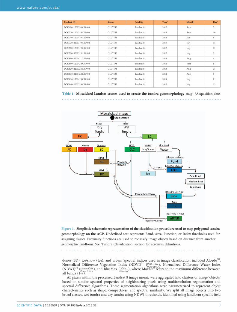
Image processingTwelve cloud free Landsat 8 satellite images were acquired during the summers of 2013 and 2014, used inthe tundra geomorphology classification (Table 1). All Landsat data products were downloaded from theUnited States Geological Survey (USGS) earth explorer web-based platform (https://earthexplorer.usgs.gov). We used only the 9 spectral bands provided by the Operational Land Imager (OLI) instrument formapping, while ignoring the 2 additional Thermal Infrared Sensor (TIRS) bands due to defective optics inthe infrared sensor28. Landsat 8 OLI spectral bands include (1) coastal/aerosol (Ultra blue), (2) blue, (3)green, (4) red, (5) near infrared (NIR), (6) shortwave infrared 1 (SWIR1), (7) shortwave infrared 2(SWIR2), (8) panchromatic, and (9) cirrus. Prior to image mosaicking, reflectance values werenormalized across satellite scenes, by calculating top-of-atmosphere reflectance29, which minimized theradiometric difference between images associated with varying atmospheric conditions, acquisition dates,and solar zenith angles29, while the Landsat Surface Reflectance Code (LaSRC) was used for atmosphericcorrection. Images were mosaicked within ArcGISTM 10.4 (ESRI).

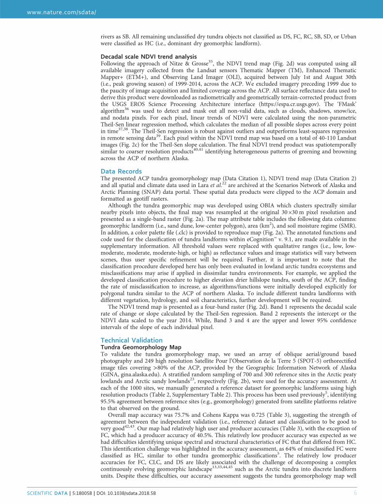
Image classificationWe expand upon geomorphic mapping procedures developed for a subregion of the ACP of northernAlaska on the Barrow Peninsula (1800 km2)5, using a novel automated object based image analysis(OBIA) approach for tundra geomorphic mapping across the ACP (58,691 km2). The OBIA land coverclassifier (eCognition™ version 9.1, Trimble) was parameterized using various rules, thresholds, spectralindices, and proximity functions using individual and combined spectral bands, spectral indices, andgeometric object shapes/sizes (i.e., perimeter, area, roundness) and corresponding reference data (i.e.,field/ground truth points and high resolution aerial/satellite imagery) to differentiate betweengeomorphic landforms (Fig. 1). Fifteen tundra geomorphic landforms were mapped at 30 × 30 m spatialresolution (Fig. 2a), including (qualitatively ranked from wet to dry), coastal saline water (CS), lakes(large:>90 ha, medium:≤ 90 and >20 ha, small:≤ 20 ha), rivers, ponds, coalescent low-center polygons(CLC), nonpatterned drained thaw lake basins (nDTLB), low-center polygons (LC), sandy barrens (SB),flat-center polygons (FC), riparian corridors (RC), high-center polygons (HC), drained slopes (DS), sand

www.nature.com/sdata/


https://earthexplorer.usgs.gov

https://earthexplorer.usgs.gov

dunes (SD), ice/snow (Ice), and urban. Spectral indices used in image classification included Albedo30,Normalized Difference Vegetation Index (NDVI)31 (ρNIR- ρRed

ρNIRþρRed), Normalized Difference Water Index

(NDWI)32 (ρGreen - ρNIRρGreenþρNIR

), and BlueMax ( ρBlueρMaxDif f

), where MaxDiff refers to the maximum difference betweenall bands (1-9).

All pixels within the processed Landsat 8 image mosaic were aggregated into clusters or image ‘objects’based on similar spectral properties of neighbouring pixels using multiresolution segmentation andspectral difference algorithms. These segmentation algorithms were parameterized to represent objectcharacteristics such as shape, compactness, and spectral similarity. We split all image objects into twobroad classes, wet tundra and dry tundra using NDWI thresholds, identified using landform specific field

Product ID Sensor Satellite Year* Month* Day*

LC80690112013249LGN00 OLI/TIRS Landsat 8 2013 Sept. 5


LC80740112014191LGN00 OLI/TIRS Landsat 8 2014 July 9




LC80800102014217LGN00 OLI/TIRS Landsat 8 2014 Aug. 4






Table 1. Mosaicked Landsat scenes used to create the tundra geomorphology map. *Acquisition date.

Figure 1. Simplistic schematic representation of the classification procedure used to map polygonal tundra

geomorphology on the ACP. Underlined text represents Band, Area, Function, or Index thresholds used for

assigning classes. Proximity functions are used to reclassify image objects based on distance from another

geomorphic landform. See ‘Tundra Classification’ section for acronym definitions.



Figure 2. Geospatial datasets representing the heterogeneity in both landform and NDVI across the ACP

of northern Alaska. The tundra geomorphology map (a) was validated with 1000 reference sites (700 and 300

in the Arctic Peaty Lowlands and Arctic Sandy Lowlands, respectively) using 249 SPOT-5 ortho-tiles (b), while

the NDVI trend map (c) was developed using between 40 to 110 image observations per 30 m pixel (d).



observations5,15. The following classification procedure (Fig. 1, Supplementary File 1), extracts all imageobjects from wet and dry tundra and reclassifies them into specific geomorphic landforms.

Wet Tundra Classification. We decomposed our classification of wet tundra into three steps, (1)extraction of CLC and nDTLB, (2) open water body differentiation, and (3) rectification ofmisclassifications. Initially, we differentiated CLC from all wet tundra objects using a low productivity(NDVI) threshold, which was associated with sparse vegetation cover and the presence of open water.Although, both CLC and nDTLB are found in aquatic to wet environments, we differentiated CLC fromnDTLB landforms using the characteristically high NDVI values of nDTLB5,15 and morphologicalfeatures. Due to the rapid formation of nDTLB following lake drainage33, this young geomorphiclandform often contains a relatively large non-polygonal surface area34 (i.e., limited effects of iceaggregation and heaving processes associated with microtopographic variability), thus we use a moderateedge to area ratio and high NDVI threshold for nDTLB feature extraction.All unvegetated open water pixels were extracted using a low-moderate blue band threshold (Fig. 1). A

spectral difference segmentation algorithm, was looped 5x to iteratively combine all neighbouring openwater objects with similar spectral properties. This object merging process enabled the identification ofeach spatially isolated water body (i.e., lake, pond, or river), where structural properties such as area,perimeter, or edge (i.e., perimeter) to area ratio can be used to differentiate waterbodies. Therefore, wedefined CS, lakes, and ponds using structural properties, area and edge to area ratio. Water bodies weredecomposed into CS (>100,000 ha) large lakes (≤ 100,000 > 90 ha), medium lakes (≤ 90 > 20 ha), smalllakes (≤ 20 >1 ha), and ponds (≤ 1 ha). The 100,000 ha area threshold was used to define CS to avoidlarge lake misclassification errors, as Teshekpuk Lake (70.61˚ N, −153.56˚ W), has an area of ~83,000 ha.Due to misclassifications of ponds as lakes, associated with the high interconnectivity between irregularlystructured open water objects, we used a low edge to area ratio on lakes, to ensure accurate classificationof ponds. Rivers were differentiated from all open water objects using a NDVI threshold and a‘roundness’ function. Integrating both approaches successfully extracted rivers, as high NDVI thresholdswere used to differentiate open water from vegetated aquatic standing water objects, and low roundnessvalues identified the characteristic elongated and meandering structure of rivers. Despite the late summerimage acquisition dates used in this classification (Table 1), ice/snow image objects identified using highSWIR2 thresholds, were found in large lakes or adjacent to steep topographic gradients such as rivervalleys or near a snow fence. All ice/snow objects that occurred on lakes were reclassified as lake area,while the remaining ice/snow was reclassified as Ice.

Although, classification functions developed for wet tundra performed well, the majority ofmisclassifications were associated with the relatively course spatial resolution object patch size (30 m).To rectify these misclassifications, we used neighborhood or proximity functions to develop relationshipsbetween nearby geomorphic landforms using spectral and structural parameters for nDTLB, CLC, pond,and lakes. For example, nDTLB was often misclassified as CLC or pond, occurring near lake perimeters.Because aquatic-wet landforms occurring near lake perimeters are typically represented by nDTLB,having recently formed after partial or complete lake drainage, we reclassified older landforms such asCLC and ponds adjacent to lakes as nDTLBs. All remaining unclassified wet tundra objects that didnot meet the criteria for nDTLB, CLC, pond, river, CS, or lakes in wet tundra were classified as LC(i.e., dominant wet geomorphic landform).

Dry Tundra Classification. We differentiated landforms in dry tundra following two steps, (1)threshold identification and extraction of FC and RC, and (2) rectification of misclassifications. A seriesof reference sites identified from ground based observations and/or oblique aerial photography were usedto define NDWI and NDVI thresholds needed to extract FC and RC, respectively. These two geomorphiclandforms were difficult to classify due to the similarity in vegetation composition and surface hydrology.However, we were able to differentiate between these two landforms, as FC was slightly higher in surfacewetness, associated with the 2 fold difference in trough area relative to HC5. The high variability in NDVIof shrub canopies in RC relative to other landforms, made RC difficult to extract. Nevertheless, becauseRC typically occurred near riverine environments, we used both a low-moderate NDVI threshold and aproximity function adjacent to rivers to extract RC. Sand and gravel objects were easily extracted using ahigh BlueMax threshold. All lightly vegetated wet-moist sand and gravel objects were classified as SBusing a moderate-high NDVI threshold, whereas drier sand and gravel objects were classified as SD. Dueto the use of sand and gravel in the development of urban infrastructure such as roads and buildings,automated procedures initially classified these feature as SD, as they had a similar spectral signature.However, we manually reclassified SD as Urban near native Alaskan villages and oil drilling platforms(i.e., near Prudhoe Bay). Although, we made significant progress with the development of classificationprocedures for Urban landforms using spectral patterns and geometric structures, we abandoned thisdevelopment due to the relatively limited area impacted by urban infrastructure across the ACP.Additionally, DS was extracted using a high albedo threshold, as this landform was very dry and oftendominated by lichen plant communities, which are highly reflective15. Similar to misclassificationsassociated with object patch size identified in wet tundra, we found analogous misclassifications of SBnear rivers as CLC and ponds. Therefore, we reclassified CLC and pond classes that were adjacent to



rivers as SB. All remaining unclassified dry tundra objects not classified as DS, FC, RC, SB, SD, or Urbanwere classified as HC (i.e., dominant dry geomorphic landform).

Decadal scale NDVI trend analysisFollowing the approach of Nitze & Grosse35, the NDVI trend map (Fig. 2d) was computed using allavailable imagery collected from the Landsat sensors Thematic Mapper (TM), Enhanced ThematicMapper+ (ETM+), and Observing Land Imager (OLI), acquired between July 1st and August 30th(i.e., peak growing season) of 1999-2014, across the ACP. We excluded imagery preceding 1999 due tothe paucity of image acquisition and limited coverage across the ACP. All surface reflectance data used toderive this product were downloaded as radiometrically and geometrically terrain-corrected product fromthe USGS EROS Science Processing Architecture interface (https://espa.cr.usgs.gov). The ‘FMask’algorithm36 was used to detect and mask out all non-valid data, such as clouds, shadows, snow/ice,and nodata pixels. For each pixel, linear trends of NDVI were calculated using the non-parametricTheil-Sen linear regression method, which calculates the median of all possible slopes across every pointin time37,38. The Theil-Sen regression is robust against outliers and outperforms least-squares regressionin remote sensing data39. Each pixel within the NDVI trend map was based on a total of 40-110 Landsatimages (Fig. 2c) for the Theil-Sen slope calculation. The final NDVI trend product was spatiotemporallysimilar to coarser resolution products40,41 identifying heterogeneous patterns of greening and browningacross the ACP of northern Alaska.

Data RecordsThe presented ACP tundra geomorphology map (Data Citation 1), NDVI trend map (Data Citation 2)and all spatial and climate data used in Lara et al.22 are archived at the Scenarios Network of Alaska andArctic Planning (SNAP) data portal. These spatial data products were clipped to the ACP domain andformatted as geotiff rasters.

Although the tundra geomorphic map was developed using OBIA which clusters spectrally similarnearby pixels into objects, the final map was resampled at the original 30 ×30 m pixel resolution andpresented as a single-band raster (Fig. 2a). The map attribute table includes the following data columns:geomorphic landform (i.e., sand dune, low-center polygon), area (km2), and soil moisture regime (SMR).In addition, a color palette file (.clc) is provided to reproduce map (Fig. 2a). The annotated functions andcode used for the classification of tundra landforms within eCognition™ v. 9.1, are made available in thesupplementary information. All threshold values were replaced with qualitative ranges (i.e., low, low-moderate, moderate, moderate-high, or high) as reflectance values and image statistics will vary betweenscenes, thus user specific refinement will be required. Further, it is important to note that theclassification procedure developed here has only been evaluated in lowland arctic tundra ecosystems andmisclassifications may arise if applied in dissimilar tundra environments. For example, we applied thedeveloped classification procedure to higher elevation drier hillslope tundra, south of the ACP, findingthe rate of misclassification to increase, as algorithms/functions were initially developed explicitly forpolygonal tundra similar to the ACP of northern Alaska. To include different tundra landforms withdifferent vegetation, hydrology, and soil characteristics, further development will be required.

The NDVI trend map is presented as a four-band raster (Fig. 2d). Band 1 represents the decadal scalerate of change or slope calculated by the Theil-Sen regression. Band 2 represents the intercept or theNDVI data scaled to the year 2014. While, Band 3 and 4 are the upper and lower 95% confidenceintervals of the slope of each individual pixel.

Technical ValidationTundra Geomorphology MapTo validate the tundra geomorphology map, we used an array of oblique aerial/ground basedphotography and 249 high resolution Satellite Pour l’Observation de la Terre 5 (SPOT-5) orthorectifiedimage tiles covering >80% of the ACP, provided by the Geographic Information Network of Alaska(GINA, gina.alaska.edu). A stratified random sampling of 700 and 300 reference sites in the Arctic peatylowlands and Arctic sandy lowlands23, respectively (Fig. 2b), were used for the accuracy assessment. Ateach of the 1000 sites, we manually generated a reference dataset for geomorphic landforms using highresolution products (Table 2, Supplementary Table 2). This process has been used previously5, identifying95.5% agreement between reference sites (e.g., geomorphology) generated from satellite platforms relativeto that observed on the ground.

Overall map accuracy was 75.7% and Cohens Kappa was 0.725 (Table 3), suggesting the strength ofagreement between the independent validation (i.e., reference) dataset and classification to be good tovery good42,43. Our map had relatively high user and producer accuracies (Table 3), with the exception ofFC, which had a producer accuracy of 40.5%. This relatively low producer accuracy was expected as wehad difficulties identifying unique spectral and structural characteristics of FC that that differed from HC.This identification challenge was highlighted in the accuracy assessment, as 64% of misclassified FC wereclassified as HC, similar to other tundra geomorphic classifications5. The relatively low produceraccuracies for FC, CLC, and DS are likely associated with the challenge of decomposing a complexcontinuously evolving geomorphic landscape13,33,44,45 such as the Arctic tundra into discrete landformunits. Despite these difficulties, our accuracy assessment suggests the tundra geomorphology map well



https://espa.cr.usgs.gov

represented the spatial distribution and heterogeneity of tundra landforms. We present for the first time,a detailed framework for characterizing arctic tundra landforms across the Pan-Arctic.

NDVI Trend MapWe evaluated the potential sensor bias between TM, ETM+, and OLI, used to derive the NDVI TrendMap by comparing the mean value for each pixel, year, and sensor computed from three differentlocations in northern Alaska (Fig. 3). Each location was composed of 40,000 pixels (~36 km2). The threecentroids of each location are found in the (1) Arctic sandy lowlands of the ACP (longitude: −154.50,latitude: 70.09), (2) foothills of the Brooks Range on the North Slope (longitude: -159.61, latitude: 66.60),and (3) Selawik lowlands in northwestern Alaska (longitude: −152.92, latitude: 69.29). Minordiscrepancies were to be expected between sensor platforms as the images were not acquired at thesame time or day.

We identified minor NDVI sensor biases between sensors (Fig. 3), while sensor specific NDVIdistributions were consistent. Most of the data used to generate the NDVI trend map was acquired fromthe ETM+ sensor, as it was available throughout our data acquisition window (i.e., 1999–2014), whereasdata from TM and OLI were only available between 2005-2011 and 2013-2014, respectively. Mean sensorbias estimates for TM and OLI across all subregions of Alaska, indicate NDVI to be slightly under- andoverestimated relative to ETM+, though the variability was high within each year and subregion (Fig. 3).

Ecological Landscape Landform Latitude Longitude

Arctic Peaty Lowland non-patterned Drained Thaw Lake Basin 71.236855 −156.3785131

Arctic Peaty Lowland High-center polygon 71.210642 −156.4676783

Arctic Peaty Lowland Pond 71.191358 −156.3469935

Arctic Peaty Lowland River 70.181085 −147.2617363

Arctic Peaty Lowland Riparian corridor 70.165456 −148.4265964

Arctic Sandy Lowland Lake 70.166375 −154.2431094

Arctic Sandy Lowland Drained slope 70.160143 −153.6316156

Arctic Sandy Lowland Sand dune 70.3493 −152.7590333

Table 2. Example of the reference dataset generated to validate the tundra geomorphology map. Thecomplete (1000 point) reference dataset can be found in the Supplementary Table 2.

Reference Sites

Geomorphic type SB SD RC DS HC FC LC nDTLB CLC Pond River Lake CS User accuracy

Classification

SB 12 2 2 1 63%

SD 3 12 2 71%

RC 4 1 80%

DS 50 19 4 69%

HC 35 215 30 22 2 70%

FC 11 32 3 71%

LC 1 6 34 11 152 5 7 2 70%

nDTLB 3 16 53 1 1 2 70%

CLC 2 2 15 2 71%

Pond 18 100%

River 2 2 2 10 63%

Lake 1 1 156 99%

CS 1 28 97%

Producer accuracy 71% 100% 80% 55% 75% 41% 77% 82% 56% 100% 83% 96% 100% 1000

Overall accuracy 76%

Cohens Kappa 0.73

Table 3. Accuracy assessment represented as a confusion matrix. Bolded diagonal values within thematrix represent correctly identified pixels, where User and Producer accuracies are presented on the rightvertical axis and bottom horizontal axis.



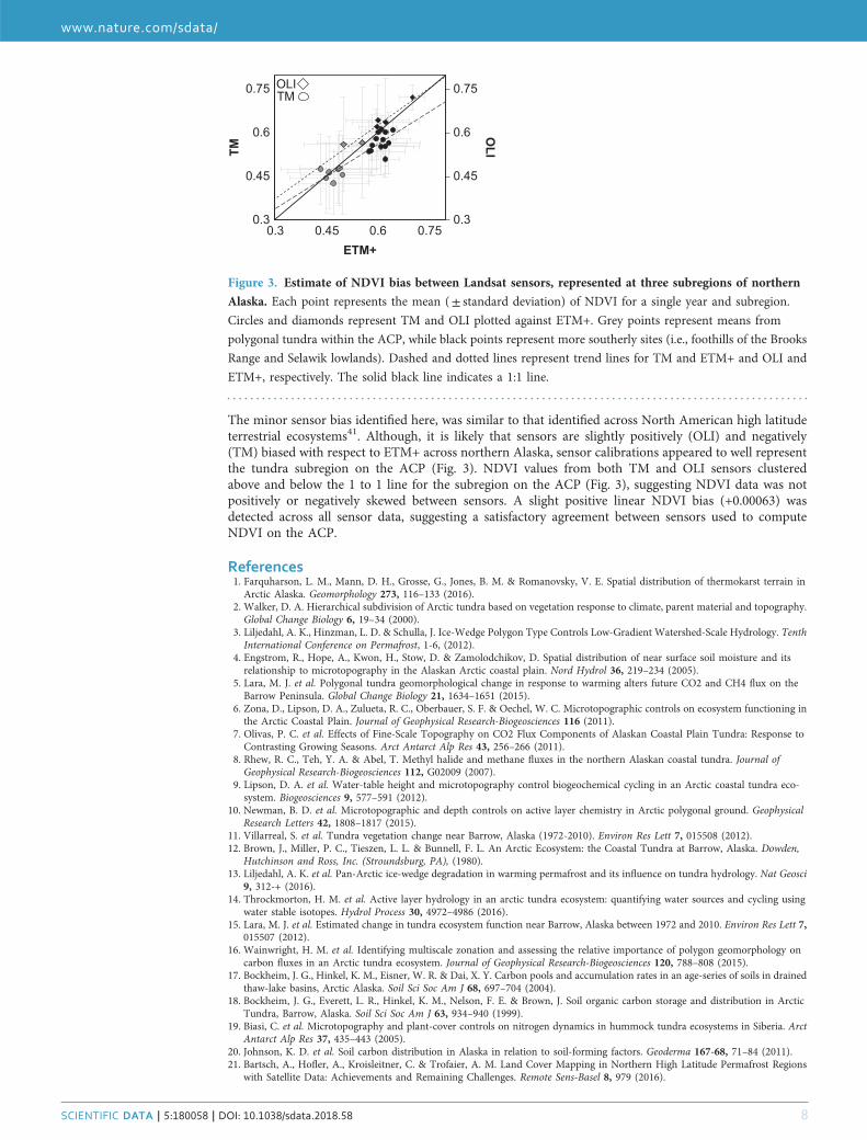
The minor sensor bias identified here, was similar to that identified across North American high latitudeterrestrial ecosystems41. Although, it is likely that sensors are slightly positively (OLI) and negatively(TM) biased with respect to ETM+ across northern Alaska, sensor calibrations appeared to well representthe tundra subregion on the ACP (Fig. 3). NDVI values from both TM and OLI sensors clusteredabove and below the 1 to 1 line for the subregion on the ACP (Fig. 3), suggesting NDVI data was notpositively or negatively skewed between sensors. A slight positive linear NDVI bias (+0.00063) wasdetected across all sensor data, suggesting a satisfactory agreement between sensors used to computeNDVI on the ACP.

References1. Farquharson, L. M., Mann, D. H., Grosse, G., Jones, B. M. & Romanovsky, V. E. Spatial distribution of thermokarst terrain inArctic Alaska. Geomorphology 273, 116–133 (2016).

2. Walker, D. A. Hierarchical subdivision of Arctic tundra based on vegetation response to climate, parent material and topography.Global Change Biology 6, 19–34 (2000).

3. Liljedahl, A. K., Hinzman, L. D. & Schulla, J. Ice-Wedge Polygon Type Controls Low-Gradient Watershed-Scale Hydrology. TenthInternational Conference on Permafrost, 1-6, (2012).

4. Engstrom, R., Hope, A., Kwon, H., Stow, D. & Zamolodchikov, D. Spatial distribution of near surface soil moisture and itsrelationship to microtopography in the Alaskan Arctic coastal plain. Nord Hydrol 36, 219–234 (2005).

5. Lara, M. J. et al. Polygonal tundra geomorphological change in response to warming alters future CO2 and CH4 flux on theBarrow Peninsula. Global Change Biology 21, 1634–1651 (2015).

6. Zona, D., Lipson, D. A., Zulueta, R. C., Oberbauer, S. F. & Oechel, W. C. Microtopographic controls on ecosystem functioning inthe Arctic Coastal Plain. Journal of Geophysical Research-Biogeosciences 116 (2011).

7. Olivas, P. C. et al. Effects of Fine-Scale Topography on CO2 Flux Components of Alaskan Coastal Plain Tundra: Response toContrasting Growing Seasons. Arct Antarct Alp Res 43, 256–266 (2011).

8. Rhew, R. C., Teh, Y. A. & Abel, T. Methyl halide and methane fluxes in the northern Alaskan coastal tundra. Journal ofGeophysical Research-Biogeosciences 112, G02009 (2007).

9. Lipson, D. A. et al. Water-table height and microtopography control biogeochemical cycling in an Arctic coastal tundra eco-system. Biogeosciences 9, 577–591 (2012).

10. Newman, B. D. et al. Microtopographic and depth controls on active layer chemistry in Arctic polygonal ground. GeophysicalResearch Letters 42, 1808–1817 (2015).

11. Villarreal, S. et al. Tundra vegetation change near Barrow, Alaska (1972-2010). Environ Res Lett 7, 015508 (2012).12. Brown, J., Miller, P. C., Tieszen, L. L. & Bunnell, F. L. An Arctic Ecosystem: the Coastal Tundra at Barrow, Alaska. Dowden,

Hutchinson and Ross, Inc. (Stroundsburg, PA), (1980).13. Liljedahl, A. K. et al. Pan-Arctic ice-wedge degradation in warming permafrost and its influence on tundra hydrology. Nat Geosci

9, 312-+ (2016).14. Throckmorton, H. M. et al. Active layer hydrology in an arctic tundra ecosystem: quantifying water sources and cycling using

water stable isotopes. Hydrol Process 30, 4972–4986 (2016).15. Lara, M. J. et al. Estimated change in tundra ecosystem function near Barrow, Alaska between 1972 and 2010. Environ Res Lett 7,

015507 (2012).16. Wainwright, H. M. et al. Identifying multiscale zonation and assessing the relative importance of polygon geomorphology on

carbon fluxes in an Arctic tundra ecosystem. Journal of Geophysical Research-Biogeosciences 120, 788–808 (2015).17. Bockheim, J. G., Hinkel, K. M., Eisner, W. R. & Dai, X. Y. Carbon pools and accumulation rates in an age-series of soils in drained

thaw-lake basins, Arctic Alaska. Soil Sci Soc Am J 68, 697–704 (2004).18. Bockheim, J. G., Everett, L. R., Hinkel, K. M., Nelson, F. E. & Brown, J. Soil organic carbon storage and distribution in Arctic

Tundra, Barrow, Alaska. Soil Sci Soc Am J 63, 934–940 (1999).19. Biasi, C. et al. Microtopography and plant-cover controls on nitrogen dynamics in hummock tundra ecosystems in Siberia. Arct

Antarct Alp Res 37, 435–443 (2005).20. Johnson, K. D. et al. Soil carbon distribution in Alaska in relation to soil-forming factors. Geoderma 167-68, 71–84 (2011).21. Bartsch, A., Hofler, A., Kroisleitner, C. & Trofaier, A. M. Land Cover Mapping in Northern High Latitude Permafrost Regions

with Satellite Data: Achievements and Remaining Challenges. Remote Sens-Basel 8, 979 (2016).

0.3

0.45

0.6

0.75

0.3

0.45

0.6

0.75

0.3 0.45 0.6 0.75

OLITM

ETM+

OLITM

Figure 3. Estimate of NDVI bias between Landsat sensors, represented at three subregions of northern

Alaska. Each point represents the mean (± standard deviation) of NDVI for a single year and subregion.

Circles and diamonds represent TM and OLI plotted against ETM+. Grey points represent means from

polygonal tundra within the ACP, while black points represent more southerly sites (i.e., foothills of the Brooks

Range and Selawik lowlands). Dashed and dotted lines represent trend lines for TM and ETM+ and OLI and

ETM+, respectively. The solid black line indicates a 1:1 line.



22. Lara, M. J., Nitze, I., Grosse, G., Martin, P. & McGuire, A. D. Reduced arctic tundra productivity linked with landform andclimate change interactions. Sci Rep 8, 2345 (2018).

23. Jorgenson, T. M. & Grunblatt, J. Landscape-Level Ecological Mapping of Northern Alaska and Field Site Photography(2013).

24. Sellmann, P. V. & Brown, J. Stratigraphy and diagenesis of perennially frozen sediment in the Barrow, Alaska, region. InPermafrost: North American Contribution to the Second International Conference. Washington, D.C.: National Academy ofSciences, 171-181, (1973).

25. Jorgenson, M. T. et al. Permafrost characteristics of Alaska. Ninth International Conference on Permafrost, 121-122,(2008).

26. Nelson, F. E. et al. Active-layer thickness in north central Alaska: Systematic sampling, scale, and spatial autocorrelation. Journalof Geophysical Research-Atmospheres 103, 28963–28973 (1998).

27. Walker, D. A. et al. The Circumpolar Arctic vegetation map. J Veg Sci 16, 267–282 (2005).28. Montanaro, M., Gerace, A., Lunsford, A. & Reuter, D. Stray Light Artifacts in Imagery from the Landsat 8 Thermal

Infrared Sensor. Remote Sens-Basel 6, 10435–10456 (2014).29. Chavez, P. S. Image-based atmospheric corrections revisited and improved. Photogramm Eng Rem S 62, 1025–1036 (1996).30. Liang, S. L. Narrowband to broadband conversions of land surface albedo I Algorithms. Remote Sens Environ 76, 213–238

(2001).31. Rouse, D. A., Haas, R. H., Schell, J. A. & Deering, D. W. Monitoring vegetation systems in the Great Plains with ERTS.

Proceedings, Third Earth Resources Technology Satellite-1 Symposium 301–317 (1974).32. Gao, B. C. NDWI- A normalized difference water index for remote sensing of vegetation liquid water from space. Remote Sens

Environ 58, 257–266 (1996).33. Jorgenson, M. T. & Shur, Y. Evolution of lakes and basins in northern Alaska and discussion of the thaw lake cycle. J Geophys Res-

Earth 112, F02S17 (2007).34. Bockheim, J. G. & Hinkel, K. M. Accumulation of Excess Ground Ice in an Age Sequence of Drained Thermokarst Lake Basins,

Arctic Alaska. Permafrost Periglac 23, 231–236 (2012).35. Nitze, I. & Grosse, G. Detection of landscape dynamics in the Arctic Lena Delta with temporally dense Landsat time-series stacks.

Remote Sens Environ 181, 27–41 (2016).36. Zhu, Z., Wang, S. X. & Woodcock, C. E. Improvement and expansion of the Fmask algorithm: cloud, cloud shadow, and snow

detection for Landsats 4-7, 8, and Sentinel 2 images. Remote Sens Environ 159, 269–277 (2015).37. Sen, P. K. Estimates of Regression Coefficient Based on Kendalls Tau. J Am Stat Assoc 63, 1379-& (1968).38. Theil, H. A rank-invariant method of linear and polynomial regression analysis. Henri Theil's Contributions to Economics and

Econometrics 23, 345–381 (1992).39. Fernandes, R. & Leblanc, S. G. Parametric (modified least squares) and non-parametric (Theil-Sen) linear regressions for

predicting biophysical parameters in the presence of measurement errors. Remote Sens Environ 95, 303–316 (2005).40. Bhatt, U. S. et al. Recent Declines in Warming and Vegetation Greening Trends over Pan-Arctic Tundra. Remote Sens-Basel 5,

4229–4254 (2013).41. Ju, J. C. & Masek, J. G. The vegetation greenness trend in Canada and US Alaska from 1984-2012 Landsat data. Remote Sens

Environ 176, 1–16 (2016).42. Fleiss, J. L., Cohen, J. & Everitt, B. S. Large sample standard errors of kappa and weighted kappa. Psychological Bulletin 72,

323–327 (1969).43. Congalton, R. G. A Comparison of Sampling Schemes Used in Generating Error Matrices for Assessing the Accuracy of Maps

Generated from Remotely Sensed Data. Photogramm Eng Rem S 54, 593–600 (1988).44. Billings, W. D. & Peterson, K. M. Vegetational Change and Ice-Wedge Polygons through the Thaw-Lake Cycle in Arctic Alaska.

Arctic and Alpine Research 12, 413–432 (1980).45. Jorgenson, M. T., Shur, Y. L. & Pullman, E. R. Abrupt increase in permafrost degradation in Arctic Alaska. Geophysical Research

Letters 33, L02503 (2006).

Data Citations1. Lara, M. J. SNAP Data Portal https://doi.org/10.21429/C9JS8S (2017).2. Lara, M. J. SNAP Data Portal https://doi.org/10.21429/C9F04D (2017).

AcknowledgementsM.J.L. was supported by the Department of Interior’s Arctic Landscape Conservation Cooperative, U.S.Department of Energy Next-Generation Ecosystem Experiments (NGEE-arctic) project, and UI School ofIntegrative Biology STEM Diversity program. I.N. and G.G. were supported by ERC #338335, HGFERC-0013, and ESA GlobPermafrost. A.D.M. was supported by a grant from the U.S. Geological Survey’sAlaska Climate Science Center. We thank Philip Martin for initial discussions that lead to theconceptualization of the polygonal tundra map. Any use of trade, firm, or product names is fordescriptive purposes only and does not imply endorsement by the U.S. Government.

Author ContributionsM.J.L. designed the study, analyzed the data, developed the polygonal tundra map, and wrote themanuscript. I.N. and G.G. developed the Landsat time series dataset. A.D.M. assisted in modelforecasting. All authors reviewed the manuscript and made significant contributions to the writing.

Additional informationSupplementary information accompanies this paper at http://www.nature.com/sdata

Competing interests: The authors declare no competing interests.

How to cite this article: Lara, M. J. et al. Tundra landform and vegetation productivity trend maps forthe Arctic Coastal Plain of northern Alaska. Sci. Data 5:180058 doi: 10.1038/sdata.2018.58 (2018).

Publisher’s note: Springer Nature remains neutral with regard to jurisdictional claims in published mapsand institutional affiliations.



http://www.nature.com/sdata

Open Access This article is licensed under a Creative Commons Attribution 4.0 Interna-tional License, which permits use, sharing, adaptation, distribution and reproduction in any

medium or format, as long as you give appropriate credit to the original author(s) and the source, provide alink to the Creative Commons license, and indicate if changes were made. The images or other third partymaterial in this article are included in the article’s Creative Commons license, unless indicated otherwise ina credit line to the material. If material is not included in the article’s Creative Commons license and yourintended use is not permitted by statutory regulation or exceeds the permitted use, you will need to obtainpermission directly from the copyright holder. To view a copy of this license, visit http://creativecommons.org/licenses/by/4.0/

The Creative Commons Public Domain Dedication waiver http://creativecommons.org/publicdomain/zero/1.0/ applies to the metadata files made available in this article.

© The Author(s) 2018



http://creativecommons.org/licenses/by/4.0/

http://creativecommons.org/licenses/by/4.0/

http://creativecommons.org/publicdomain/zero/1.0/

http://creativecommons.org/publicdomain/zero/1.0/

tundra landform and vegetation productivity trend maps for

Documents