tullock contests of weakly heterogeneous players

Tullock Contests of Weakly Heterogeneous PlayersAuthor(s): Dmitry RyvkinSource: Public Choice, Vol. 132, No. 1/2 (Jul., 2007), pp. 49-64Published by: SpringerStable URL: http://www.jstor.org/stable/27698126 .

Accessed: 16/06/2014 09:46

Your use of the JSTOR archive indicates your acceptance of the Terms & Conditions of Use, available at .http://www.jstor.org/page/info/about/policies/terms.jsp

.JSTOR is a not-for-profit service that helps scholars, researchers, and students discover, use, and build upon a wide range ofcontent in a trusted digital archive. We use information technology and tools to increase productivity and facilitate new formsof scholarship. For more information about JSTOR, please contact [email protected].

.

Springer is collaborating with JSTOR to digitize, preserve and extend access to Public Choice.

http://www.jstor.org

This content downloaded from 195.34.79.174 on Mon, 16 Jun 2014 09:46:45 AMAll use subject to JSTOR Terms and Conditions

http://www.jstor.org/action/showPublisher?publisherCode=springer

http://www.jstor.org/stable/27698126?origin=JSTOR-pdf

http://www.jstor.org/page/info/about/policies/terms.jsp


Public Choice (2007) 132:49-64

DOI 10.1007/slll27-006-9133-x

ORIGINAL ARTICLE

Tullock contests of weakly heterogeneous players

Dmitry Ryvkin

Received: 24 January 2005 / Accepted: 21 December 2006 / Published online: 18 January 2007

? Springer Science + Business Media B.V. 2007

Abstract I explore asymmetric equilibria in a Tullock contest of heterogeneous players

in the case when the players' heterogeneity is weak, and the effort optimization problem can be analyzed in the linear approximation. With increasing discriminatory power of the

contest, players sequentially drop out. The corresponding threshold values of the discrimi

natory power are related to those identified earlier for a Tullock contest of identical players. Weak heterogeneity, however, is sufficient to make the players' behavior strongly asymmet

ric and qualitatively alter the structure of the equilibria as compared to the homogeneous case.

Keywords Contests Rent-seeking Heterogeneous players

JEL Classification: C72, D72

1 Introduction

A contest happens when several players (individuals or groups) compete for a prize by expend

ing effort or other resources. The very generic notion of a rent-seeking contest (Krueger, 1974)

can be applied to a variety of conflict situations, including R&D competition (Taylor, 1995;

Baye & Hoppe, 2003), elections (Strumpf, 2002), lobbying (Bos, 2004), sports (Szymanski, 2003) and labor market tournaments (Prendergast, 1999).

In imperfectly discriminating contests, expending the highest level of effort does not

guarantee a win.1 In contest models, starting from Tullock (1980), this ambiguity is captured

by a contest success function (CSF), which is defined as the probability for a player to win

1 Intuitively, the reason is that effort does not translate unambiguously into an observable output; instead, an

intermediate stage is involved that probabilistically favors players who exert higher effort, but still leaves a

(smaller) chance of winning for players who exert lower effort. In the limit of perfect discrimination (which occurs, for example, in all-pay auctions), the player with the highest effort always wins.

D. Ryvkin

Department of Economics, Florida State University, Tallahassee, FL 32308, USA

e-mail: [email protected]

ta Springer



50 Public Choice (2007) 132:49-64

the contest, given effort levels of all participating players. Suppose there are N players, and

their effort levels are e, > 0, i = 1, ..., N. The CSF proposed by Tullock (1980) has the

form,

Pi(eu---,eN)=-??;. (1)

A/=i eJ

Here P? denotes the winning probability for player i as a function of her and all other players'

effort levels. Parameter y > 0 is the discriminatory power of the contest, which determines

how much impact a player's own effort has on her winning probability.

Although CSF (1) was initially introduced somewhat arbitrarily, it was later shown by Skaperdas (1996) and Kooreman and Schoonbeek (1997) that under fairly general conditions it is the only possible CSF, which makes its detailed analysis meaningful.2 More general forms

of the CSF (such as those used by, for example, Szidarovszky & Okuguchi, 1997; Cornes &

Hartley, 2005) can also be analyzed within the framework presented here. I choose the CSF

(1) for illustrative purposes, since it is conveniently characterized by a single parameter y.

It is also arguably the most popular CSF in the literature.

Let V denote the common prize value. Payoff of a (risk-neutral) player / can be written

in a separable form as

eY

7t'=V^?-V~c'e^ ? = !,...,#, (2)

?/ = ! ei

where c? is the effort cost parameter of player /. Specification (2) describes heterogeneous costs of effort.3 I will henceforth refer to c? as player / 's ability, keeping in mind that under

specification (2) larger c? corresponds to lower ability. In the simplest one-period simultaneous-move contest game, players commit to certain

effort levels, and their payoffs are given by Equation (2). For identical players, P?rez-Castrillo

and Verdier (1992) described possible pure strategy equilibria of this game. When discrimina

tory power y is sufficiently low, all players exert the same positive effort, and the equilibrium

is symmetric. However, for y beyond certain threshold value asymmetric equilibria are iden

tified, in which some of the players exert positive effort, while others exert zero effort (drop

out).4

For heterogeneous players, earlier work on the Tullock contest is summarized by Lockard

and Tullock (2001). The results are either purely numerical (Allard, 1988), or only regard

particular cases o? N = 2 players (Nti, 1999; see also Dixit, 1987 & Baik, 1994 for more

general treatment of the two-players case), or discriminatory power y = 1 (Nitzan, 1991).

More recent studies continue along the same lines. They are either very general, with only

qualitative conclusions (see e.g. Singh & Wittman, 2001 ; Cornes & Hartley, 2005), or consider

specific values of N = 2 and/or y ?

1. For example, see Malueg and Yates (2004) for the

2 Different sets of assumptions regarding the "contest technology" lead to different forms of the CSF. For details, see Skaperdas (1996); see also Skaperdas (1992) and Epstein and Nitzan (2006) for a micro foundation of some of these assumptions. 3 Alternatively, players' heterogeneity can be introduced through asymmetric prize valuations (e.g. Nti, 1999)

or asymmetries in the CSF itself (e.g. Cornes & Hartley, 2005). For the analysis presented below it is only

important that each player be characterized by a single heterogeneity parameter c?. 4

Baye, Kovenock, and de Vries (1994) describe a symmetric equilibrium in mixed strategies for the case of

y > 2, when no equilibria in pure strategies exist.

*__ Springer



Public Choice (2007) 132:49-64 51

case of N = 2 players; Stein (2002), Epstein and Nitzan (2002), and Stein and Rapoport (2004) assume y

= l.5

What lacks in the literature is a detailed quantitative analysis of equilibria with heteroge neous players, which would show explicitly how the heterogeneity, the number of players,

and the discriminatory power jointly determine possible equilibrium configurations. The

analysis of Cornes and Hartley (2005) partially fills this gap, but still proposes only the

"existence-and-inequalities" type of results, which is not surprising given the generality of

the approach taken. Here, I present a much less general but more explicit and quantitative

analysis of this long-standing problem.

In this paper I analyze the Tullock contest of heterogeneous players for arbitrary number of

players N and discriminatory power y < 2 for the case when the heterogeneity of players is,

in a well-defined sense, weak. Suppose players' abilities are different but closely concentrated

around some average value. Then, under certain conditions, their equilibrium effort levels

will also be different but closely concentrated around the corresponding equilibrium effort

levels for the case of identical players with the average ability.6 I explicitly derive conditions

under which different equilibrium configurations are sustainable.

When payoffs are sufficiently smooth functions of players' actions, weak heterogeneity is

tractable mathematically by Taylor-expanding the first-order conditions around a symmetric

equilibrium point. The accuracy of the resulting approximation depends on the order of the

expansion. This approach was used by Akerlof and Yellen (1985) in their study of the impact of weak irrationality of agents on the market equilibrium, and also by Fibich et al. (2004) for

auctions.7

It is interesting to study weak heterogeneity for several reasons. In practice players are

always at least slightly heterogeneous. On the other hand, the behavior of identical players is often well understood theoretically. Therefore, it is important to know how robust an

equilibrium with identical players is with respect to small heterogeneity. Will the players' behavior change dramatically? Will there be a qualitative change in the structure of equilibria?

As a result of such analysis, I show that the structure of equilibria in the Tullock contest

is, to a certain extent, preserved when weak heterogeneity of players is added. However, I

also identify a threshold beyond which heterogeneity leads to a breakdown of the structure of

equilibria. Importantly, this threshold can still be identified within the linear approximation. For numerical illustration, I control for the accuracy of the linear approximation by comparing its results with those of a high-precision numerical solution of the complete problem.

The paper is organized as follows. The general formulation of the problem is given in

Section 2. Section 3 summarizes, for future references, properties of the equilibrium for the

case of identical players. Section 4 introduces the linear approximation and characterizes

the equilibrium for weakly heterogeneous players with all players participating. Section 5

describes equilibria where part of the players drop out. Section 6 contains a numerical example for a particular configuration of players' heterogeneity. Discussion and conclusions are given in Section 7.

5 For N = 2 and/or y = 1 the problem is exactly solvable. Additionally, the case of y = 1/2 can be solved

exactly for N = 3, 4. No other exactly solvable cases are known. 6 In fact, as will be shown below, very small heterogeneity may lead to dramatic differences in efforts. 7 Note that the weak heterogeneity in this context does not mean "almost zero", in the trembling-hand sense.

The analysis below works for various degrees of heterogeneity, generally significantly different from zero (say, 10%). The weakness assumption is only needed to linearize the otherwise nonlinear first-order conditions for

optimal effort levels. The corresponding limits of validity of the linear approximation are also consistently derived.

:__ Springer



52 Public Choice (2007) 132:49-64

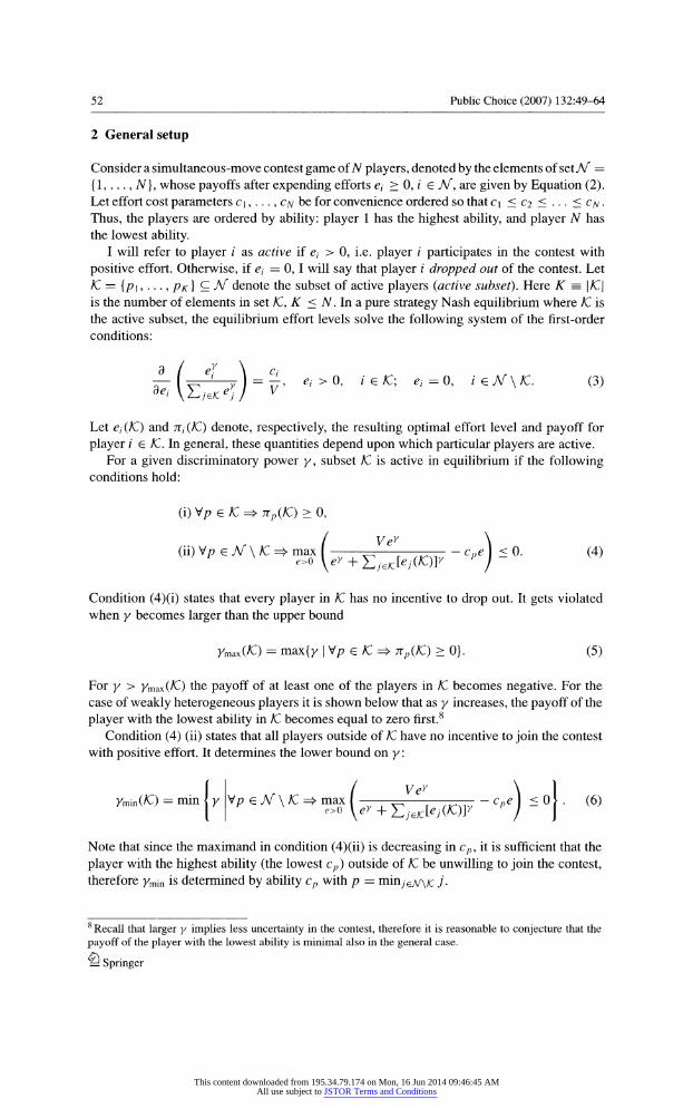
2 General setup

Consider a simultaneous-move contest game of N players, denoted by the elements of set J\f ?

{1, ..., N}, whose payoffs after expending efforts a > 0, / G Ai, are given by Equation (2).

Let effort cost parameters c\, ..., c/v be for convenience ordered so that c\ < c2 < .. < c#

Thus, the players are ordered by ability: player 1 has the highest ability, and player N has

the lowest ability.

I will refer to player / as active if e? > 0, i.e. player / participates in the contest with

positive effort. Otherwise, if e? = 0,1 will say that player / dropped out of the contest. Let

JC = {pi,..., pk} -A? denote the subset of active players (active subset). Here K =

|/C|

is the number of elements in set JC, K < N. In a pure strategy Nash equilibrium where JC is

the active subset, the equilibrium effort levels solve the following system of the first-order

conditions:

d I ey \ c

Let e? (JC) and tt? (JC) denote, respectively, the resulting optimal effort level and payoff for

player / e /C. In general, these quantities depend upon which particular players are active.

For a given discriminatory power y, subset /C is active in equilibrium if the following conditions hold:

(i)VpeJC=>7Tp(rC)>0.

(ii) VpeAf\JC=*max[ t ̂ / c'r ̂ ^ - cpe )

< 0. (4) Ve*

Condition (4)(i) states that every player in /C has no incentive to drop out. It gets violated when y becomes larger than the upper bound

)W(/0 = max{)/ | Vp g K => np(rZ) > 0}. (5)

For y > ymSLX(JC) the payoff of at least one of the players in /C becomes negative. For the

case of weakly heterogeneous players it is shown below that as y increases, the payoff of the

player with the lowest ability in /C becomes equal to zero first.8

Condition (4) (ii) states that all players outside of /C have no incentive to join the contest with positive effort. It determines the lower bound on y :

Ymm(rC) = min { y Vey

V/7 e Ai \ /C =? max ( ^- /^iv

- cpe J

< 0 (6)

Note that since the maximand in condition (4)(ii) is decreasing in cp, it is sufficient that the

player with the highest ability (the lowest cp) outside of /C be unwilling to join the contest, therefore ymm is determined by ability cp with p =

miny ^\^ j.

8 Recall that larger y implies less uncertainty in the contest, therefore it is reasonable to conjecture that the

payoff of the player with the lowest ability is minimal also in the general case.

ta Springer



Public Choice (2007) 132:49-64 53

Thus, the equilibrium with active subset /C exists for

ymm(rC) < y < )w(/C). (7)

In the case of identical players, where possible active subsets /C can be completely char

acterized by the number K of active players, the equilibrium effort levels, as well as the

equilibrium numbers of active players, and the threshold values of y, have been found earlier

(see, e.g., P?rez-Castrillo & Verdier, 1992). For completeness, I discuss the case of identical

players in Section 3. For weakly heterogeneous players, I find the corresponding quantities

in Sections 4, 5.

3 The case of identical players

This section contains a summary, for future references, of the analysis of the Tullock contest

of identical players. It repeats the results of P?rez-Castrillo and Verdier (1992), except for

the values of y^n(K),

the lower bounds on y for the existence of an asymmetric equilibrium

of K < N active players, that are new.

Suppose first that all N players actively participate in the contest, e? > 0, / e Ai. We also

assume that y < 2 in order to avoid the situation where no pure strategy equilibria exist. Let

c denote the homogeneous cost parameter. The payoff of player / is given by Equation (2) with Ci = c, and the solution to the system of the first-order conditions, dTCj/dei

= 0, / =

1, ..., N, gives the symmetric equilibrium effort level

The corresponding optimal payoff of every player is

y(N -

1) V 7T*(N)

= ?

N 1 (9) AT

As seen from Equation (9), all N players are active provided

y<yZW)> yZW) = j^j-

(10)

When constraint (10) is violated, players start dropping out. Suppose K < N players are

active, and the remaining N ?

K players exert zero effort. Then the equilibrium effort and

payoff levels of active players are e*(K) and tt*(K), as given by Equations (8) and (9),

respectively. The payoff of active players must remain non-negative, i.e. y < y^x(K)

must

hold. Equation (6) gives the lower bound on y for the existence of an equilibrium with K

active players; it becomes, after some transformations,

( yy y(K-l)y\ max -?-?- = 0. (11) y>0 \yY +K K2 J

ta Springer



54 Public Choice (2007) 132:49-64

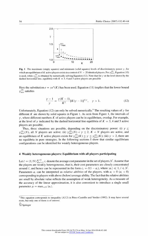
Fig. 1 The maximum (empty squares) and minimum (solid squares) levels of discriminatory power y, for

which an equilibrium of AT active players exists in a contest of N > 20 identical players. For >?ax, Equation (10)

is used, while y^n is obtained by numerically solving Equation (12). Note that for y at the level shown by the

dashed horizontal line, equilibria with K = 3,4 and 5 active players are possible

Here the substitution e = ye*iK) has been used. Equation (11) implies that the lower bound

/0). 'min

Y - 1 Y(K-?)

Y K2 [K(y -

1)] i/y y>l. (12)

Unfortunately, Equation (12) can only be solved numerically.9 The resulting values of y for

different K are shown by solid squares in Figure 1. As seen from Figure 1, the intervals of

y, where different numbers K of active players can be in equilibrium, overlap. For example,

at the level of y indicated by the dashed horizontal line equilibria of K = 3, 4 and 5 active

players are possible.

Thus, three situations are possible, depending on the discriminatory power: (i) y <

Yma*(N), all N players are active; (ii) y^xiN) < y < 2, K < N players are active, and

an equilibrium of K active players exists for y^n(K) < y <

y^xiK); (iii) y > 2, there are

no equilibria in pure strategies. In the following sections I show that similar equilibrium

configurations can be identified for weakly heterogeneous players.

4 Weakly heterogeneous players: Equilibrium with all players participating

Let c = ( 1 /N) Yli=\ ci denote the average cost parameter in the set of players J\f. Assume that

the players are weakly heterogeneous, that is, their cost parameters are closely concentrated

around c, and hence can be represented in the form c? ?

cil ?

a?), where \a? | < 1, / M.

Parameters a? can be interpreted as relative abilities of the players, with a? > 0 ia? < 0)

corresponding to players with above (below) average ability. The fact that the relative abilities

are small by absolute value reflects the assumption of weak heterogeneity. As a measure of

the accuracy of the linear approximation, it is also convenient to introduce a single small

parameter ?jl = max/ ^ \a?\.

9This equation corresponds to inequality (A3.2) in P?rez-Castrillo and Verdier (1992). It may have several

roots, but only one of them is of interest.

1__ Springer



Public Choice (2007) 132:49-64 55

Let ?N ? (l/N) Y^f=\ e? denote the (arbitrary a priori) average equilibrium effort. Then

it is natural to look for the equilibrium efforts in the form e? = ?N(l + x,), where \x?\ <<C 1

are (unknown) relative efforts. The idea is intuitive: small heterogeneity in abilities can only

lead to small heterogeneity in efforts. One needs to be careful, however, because it is not

clear a priori that the resulting relative efforts will be small without additional constraints

on parameters. Particularly, some of the players may drop out of the contest because of even

small heterogeneity. Therefore, after having obtained the equilibrium relative effort levels

one needs to go back and derive the conditions under which they remain small.

With all N players actively participating in the contest, Equations (3) take the form

er'(E^<7er)--^, i eX. (13)

At this point we linearize the generally nonlinear equations (13) for the equilibrium effort

levels. Substituting the representations c? = c(l

? a?), e? =

?/v(l + x?) into Equations (13)

and using Taylor expansions up to the linear order in x, and a? leads to

[1 + (y -

!)*, ][??_.(! + yxj)

- (1 + yx,)] ?Nc(l-a,) . Kf

--z-=-, i e M. (14)

[E?L,a + yx;)]2 yy

Here and below, unless noted otherwise, all equations involving the relative equilibrium effort

levels x? are assumed to hold with accuracy 0(p?).

For convenience, introduce X = $^/_=i */ The next step is to transform Equations (14)

into a linear form by neglecting all terms of order higher than linear in a? and x, :

CnC n o N -l + yX-yxi+(N- \){y

- l)x, -

t~-(N2 + 2NyX -

N2a?), i e M. (15) Vy

There are two kinds of terms in Equations (15): small terms proportional to x?, X, and a?,

and large terms that do not contain the small parameters. Clearly, the two groups of terms

must satisfy the equations independently because small terms can not cancel large terms.

Therefore ?^ must be chosen so that

eNcN2 N-l =

-^-?. (16)

Vy

As expected, eN given by Equation (16) is the same as the optimal effort level e*(N) in the

homogeneous case, Equation (8), provided c is the homogeneous cost parameter.

Using Equation (16) and equating the remaining terms in Equations (15) yields

(?*-) YX + [(N -l)(y-l)-y]Xi=(N

-Di^X-aA, ieM. (17)

Now sum up all Equations (17) and introduce average relative ability <5/v = (l/N) 2^1, a, .

This leads to

NyX + [(N -

l)(y -

1) -

y]X = (N -

l)(2yX -

NaN), ?? Springer



56 Public Choice (2007) 132:49-64

and finally, after elementary transformations, X = NaN. Then from Equations (17),

<eA/\ (18) ..N-2

ai ?

Y~M^\aN

1 y n-\

The result looks very appealing intuitively: relative effort x? is a weighted average of player

/'s relative ability, a?, and average relative ability, a^. Note that relative abilities a? are

constructed in such a way that ?# = 0. This is no longer the case, however, when players

start dropping out, which is the reason why ?^ is kept in Equation (18).10

Of interest are the quantities

Cj de? dx?

e? dcj daj ' e??

= --J-^L

= ^L, (19)

which are the elasticities of effort with respect to ability. Player / 's own elasticity Su = e

and cross elasticity ?/; = s (i /y) are

l-y. N-2

N(N-\) . ~( . _ Y N(N-l) . ~, , /om

1 Kiv-i 1 ^/v-i

The accuracy of these expressions is 0(?jl) because of the differentiation taking place in

Equation (19). In this approximation the elasticities are constant across players. Remarkably,

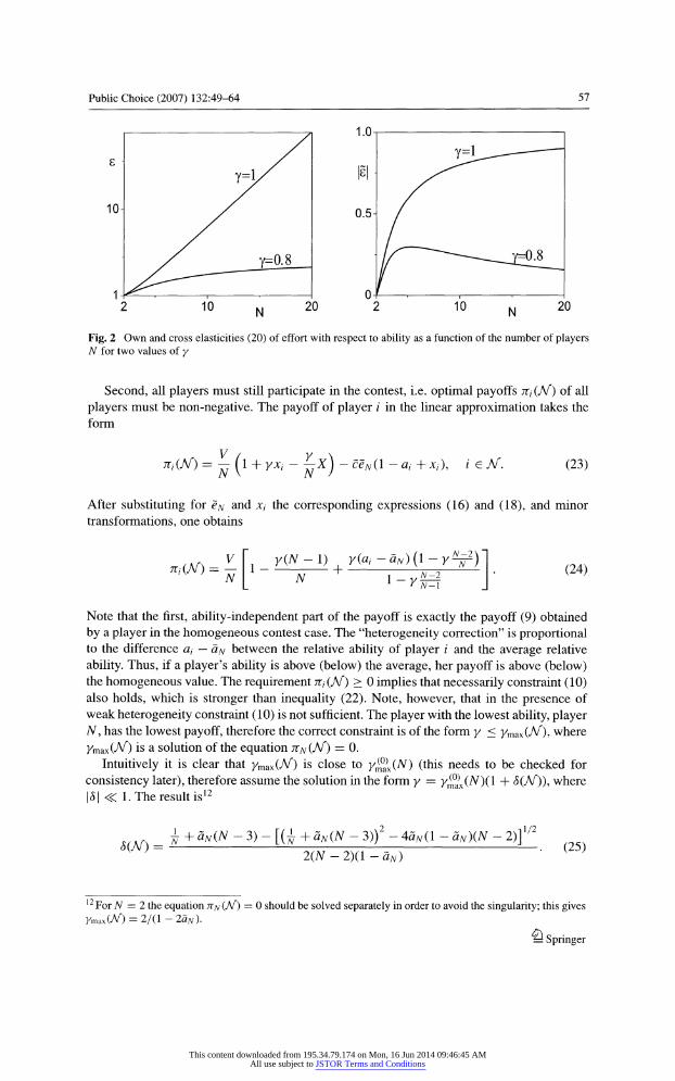
for any Af and y (such that still all TV players are active) own elasticity s > 1, i.e. the players' reaction to small changes in their own relative advantage is strong. It is also seen from

Equation (20) and Figure 2 that s increases with Af and y, i.e. the larger is the number of rivals and/or the discriminatory power, the more aggressively the players change their

effort in response to a change in their relative advantage. Cross elasticity s is negative for

N >3 and equals zero for N = 2. It is known (Nti, 1999) that in the case of two players the sign of the cross elasticity depends on the players' abilities, i.e. the accuracy 0(?x) is

not sufficient to capture it. However, it follows from Equation (20) that for A^ > 3 the cross

elasticity is negative for sufficiently weak heterogeneity. Also, \e\ < 1, i.e. a player's reaction

to information about other players' abilities is not that strong.

Relative equilibrium efforts x?, Equation (18), must be checked for self-consistency. First,

they are supposed to remain small, i.e.

kl?l-K^^, ieAT- (21)

When discriminatory power y is small, this constraint is not restrictive (recall that \a? \ <?. 1 is assumed anyway), but when y becomes larger, the range of "allowed" heterogeneity shrinks.

When y =

(N ?

l)/(N ?

2), no heterogeneity is allowed. Thus, an additional constraint is11

N -

1 y < -. (22) Y N-2 K J

10 Equation (18) can also be obtained by writing x? =

J2jeAf^Xi/^aj)aj + Oi^), where the derivative is

evaluated for a, = 0, i e N, by implicitly differentiating Equation (13). 11

Fortunately, the equilibrium of N active players ceases to exist before this constraint is violated; see below.

t? Springer



Public Choice (2007) 132:49-64 57

Fig. 2 Own and cross elasticities (20) of effort with respect to ability as a function of the number of players N for two values of y

Second, all players must still participate in the contest, i.e. optimal payoffs 7ti(Ai) of all

players must be non-negative. The payoff of player / in the linear approximation takes the

form

m(N) V

? (l + yx?

- ?X)

- ceN(l -ai + x?), i e Ai. (23)

After substituting for eN and x? the corresponding expressions (16) and (18), and minor

transformations, one obtains

*CA0 = ^

y(N -

1) y(al

N + -?N){\-Y*jft 1 y

? (24)

Note that the first, ability-independent part of the payoff is exactly the payoff (9) obtained

by a player in the homogeneous contest case. The "heterogeneity correction" is proportional to the difference a?

? ?N between the relative ability of player / and the average relative

ability. Thus, if a player's ability is above (below) the average, her payoff is above (below) the homogeneous value. The requirement 7T?(Ai)

> 0 implies that necessarily constraint (10)

also holds, which is stronger than inequality (22). Note, however, that in the presence of

weak heterogeneity constraint (10) is not sufficient. The player with the lowest ability, player

N, has the lowest payoff, therefore the correct constraint is of the form y < ymSLX(Ai), where

Ym<ix(Ai) is a solution of the equation tvn(A?) = 0.

Intuitively it is clear that ymax(Ai) is close to y^x(N) (this needs to be checked for

consistency later), therefore assume the solution in the form y = y^(N)(l + 8(Ai)), where

\8\ < 1. The result is12

S(M) = ? + ?N(N -

3) -

[(? + ?N(N -

3))2 -

4?N(l -

?N)(N -

2)] 2(N-2)(l-?N)

1/2

(25)

12 For iV = 2 the equation 7i^(J\?) = 0 should be solved separately in order to avoid the singularity; this gives

KmaxCA0 =

2/(l-25tf).

ta Springer



58 Public Choice (2007) 132:49-64

Here ?N ?

a^ ?

?N is the relative ability of the worst player in ?? counted off the average

relative ability. As expected, 8 < 0, i.e. players start dropping out at a smaller y compared

to the homogeneous case.

5 Weakly heterogeneous players: Equilibria with less than N players participating

It is seen formally from Equation (24), and also clear intuitively, that payoffs are higher

for players with higher abilities. Consequently, as discussed in the previous section, the

equilibrium of TV actively participating players ceases to exist when the payoff of the player

with the lowest ability becomes negative. At this point one of the players, player pN, drops

out of the contest. The remaining N ?

I players then find themselves in the situation similar

to the one discussed in previous section. As y increases further, some other player p/v-i

drops out, and so on, until only two players, J\f \ {pN, /?/v-i, ..., p3], remain.

Consider an intermediate equilibrium after N ?

K drop-outs, 2 < K < N, in which play

ers JC = {p\, ..., Pk } are active, while players {pk+\ , , Pn} have dropped out. For play

ers in a subset JC, the average homogeneous effort eK, as given by Equation (16), should

be used as the reference effort, i.e. the unknown equilibrium effort should be written in the

formc/(/C) = eK(l + x?(JC)). Further, let ?(/C) = (l/^)X??e/c^ denote the average relative

ability in a subset JC, with ?(M) = aN. Then, following the same logic as in the previous

section, the equilibrium relative effort levels of the active players will be [cf. Equation (18)]

XiiJC) = -^2?'

' e JC- <26) 1

~~ y~i<^\

The payoffs of the active players become (cf. Equation (24))

V 7T,(/C)=

? YJK - 1) Yi?i-a(K))(\-YW / e rZ. (27)

Let us now identify the conditions under which subset /C will be active in equilibrium.

As before, the technical condition for the linear approximation to work is \a?: | <^ 1 ?

yiK ?

2)/(K ?

I), i e JC, which implies, in particular, y < iK ?

l)/iK ?

2), similarly to condition

(22). It also must be that no player in JC is willing to drop out and no other player is willing

to join the contest, i.e. conditions (4) must hold. Let piiB) =

ma.xke?k denote the player

with the lowest ability in a subset B ? J\f (recall that the players in J\i are ordered so that

higher numbers correspond to lower abilities). Using Equation (25), the expression for the

upper bound on y can be written immediately as ymaxiJC) = y^xiK)il + 5(/C)), with (cf.

Equation (25))

?r, Y + ?Pl{K){K -

3) -

[(1 + ?PliJO(K -

3)f -

4?PliJC)(l -

?MK))(K -

2)]1/2 ?(/C)

= -

2(K-2)(l-?MK))

Here ?pi(jc) =

aPl(K) ~

aiJC)\ the correction is always negative, as before.

%? Springer

(28)



Public Choice (2007) 132:49-64 59

-0.5

-0.6

2 10

Fig. 3 Function <fi(K), as given by Equation (31)

Further, let ph (B) =

min? # k denote the player with the highest ability in a subset B ? Af.

According to Equation (6), the lower bound on y is the solution of the equation

vey

e>o \ey +K?YK(l + y?(K.)) :(1 -aPl?M\K))e)

=0 (29)

The same steps as in the case of identical players lead to the following equation for ymin(/C)

(cf. Equation (12)):

y - 1

= y(K -

1)

y K2 (\-aPh{N^))[K(y-\)(\ + y?(JC))} Wy (30)

The solution of Equation (30) is close to y^n(K), the solution of Equation (12). It can,

therefore, be sought approximately in the form y = y^?(K)(l + rj), where small parameter

r? is linear in aPh{^\K) and a(JC). This gives

Knin(/Q = yZ(K) [1 + <t>(K) (?(JC)

- ap??NxK))],

(p(K) =

HK(yZ(K)-D]-yZ(K) (31)

Function (p(K) is shown in Figure 3. As seen from the Figure, (j)(K) < 0, therefore the sign of the heterogeneity correction in ym?n(/C) depends on the sign of the difference a(JC)

- aPh^\?o.

Recall that aPh^\)C) is the relative ability of the best player outside of JC, therefore the

correction is positive if the best player outside of JC has a higher ability than the average

ability in JC, and negative otherwise.

6 Numerical illustration

In this section I illustrate the theory developed above by a numerical example. I make

the illustration by directly comparing the results of the approximate theory, as given by the analytical formulas obtained in Sections 4 and 5, with the results of exact numerical

ta Springer



60 Public Choice (2007) 132:49-64

0.00

0.05 H 0.10 0.00 0.05 h 0.10

Fig. 4 The equilibrium relative efforts (left), equilibrium payoffs (middle), and the maximal level of y (right) for N = 4 weakly heterogeneous players, as functions of heterogeneity parameter d. Discriminatory power

y = 0.8 is used in the left and middle panels. Solid lines show analytical results [Equations (18), (24) and

(25), respectively], while solid squares are the results of exact numerical calculations

calculations.13 Overall, the agreement is very good as long as the players' heterogeneity

remains weak, which leads to the conclusion that the approximate theory and its implications are reliable.

Consider a contest of weakly heterogeneous players with average cost of effort c = 1 and

prize V = 1. For simplicity, assume that relative abilities a? are uniformly distributed along

the interval (?d,d), where d <^C 1. Formally, set

a? JV + 1-21

iV + 1 (32)

Thus, d is the measure of the players' heterogeneity; the case of identical players corresponds to d = 0. In the example below I use N = 4.14

Let ?? = {1, 2, 3, 4}. First consider the case when all 4 players are active. Figure 4 shows

the results for y = 0.8. The agreement between the analytical results of Section 4 (solid

lines) and exact numerical calculations is very good, at least up to d = 0.1.

Equilibrium relative efforts x? as functions of d are shown in the left panel of Figure 4.

They start from x? = 0 for d = 0, that is, all effort levels are equal to the average equilibrium

effort ?4 = (4 ?

l)/42 0.8 = 0.15 (cf. Equation (8)). As d increases, the efforts of the two

players, whose abilities are above (below) the average, increase (decrease) with respect to the

average effort. The reaction to heterogeneity is strong, as predicted by large own elasticity e~

(20).

Equilibrium payoffs n? as functions of d are shown in the middle panel of Figure 4.

They behave similarly to the equilibrium relative efforts, starting from the homogeneous

value 7T* = (1/4)(1 - 0.8 3/4) = 0.1 for d = 0 (cf. Equation (9)) and splitting for d > 0.

Players with higher (lower) abilities enjoy higher (lower) payoffs. The equilibrium of 4 active players exists for 0 < y < ymax(Af)9 and the right panel of

Figure 4 shows KmaxCA/") as a function of d. It takes the well-known value of 4/3 for d = 0,

and decreases monotonically with d. Indeed, adding heterogeneity makes the equilibrium

13 By "exact" numerical calculations I mean numerical solutions of Equation (13) and other relevant equations,

that do not use the linear approximation. The accuracy of these calculations is only limited by the precision of Mathematical FindRoot procedure that I used.

14 The value of N = 4 is not too large, so the behavior of players is easy to intuit, at least qualitatively; on the

other hand, N = 4 is already sufficient to demonstrate the power of the linear approximation, since there is

no exact analytical solution for this N in the general case.

A\ ?_ Springer



Public Choice (2007) 132:49-64 61

J ?2'3'4?

0.00 0.05 0.10 0.00 0.05 0.10

Fig. 5 The ranges of discriminatory power y where equilibria with active subsets {1, 2, 3} (left) and {2, 3, 4}

(right) exist. The upper bound for the equilibrium with full participation is shown in both panels. Solid lines

show analytical results [Equations (31), (28), (25)], while solid squares are the results of exact numerical

calculations

more vulnerable, as the payoffs of the players with lower abilities become equal to zero for

smaller y than on average.

Let us now look at the case when less than 4 players are active. Suppose first that player

4 drops out, i.e. the active subset is {1, 2, 3}. The left panel of Figure 5 shows how the

range of y where an equilibrium of active players {1, 2, 3} exists changes with d. The

upper bound ymax({l, 2, 3}) starts at 3/2 for d = 0 and decreases monotonically. The lower bound Kmin({l, 2, 3}) starts at its homogeneous value 1.165 (cf. Figure 1) and also decreases with d. As seen from Equation (31), this happens because the player who dropped out

(player 4) has a lower ability than the average ability in the active subset. The left panel of Figure 5 also shows the upper bound ymax({l, 2, 3, 4}) for the equilibrium of 4 active

players (it is shown separately in the right panel of Figure 4). Between the two lowest curves the equilibrium with full participation and the equilibrium with player 4 dropping out coexist.

Suppose, instead, that player 1 drops out, i.e. the active subset is {2, 3,4}. The correspond

ing upper and lower bounds on y are shown in the right panel of Figure 5, together with the upper bound on full participation ymax({l, 2, 3, 4}). Here, the lower bound ymjn({2, 3, 4}) increases with d, which reflects the fact that the player who dropped out (player 1) has a

higher ability than the average ability in the active subset. As a result, ymin({2, 3, 4}) and

ttnaxiU, 2, 3, 4}) intersect at some d (shown by the dashed vertical line). This means that for d to the right of the dashed line there is an expanding range of y where an equilibrium with full participation no longer exists, but an equilibrium with active subset {2, 3, 4} also does not exist. The former equilibrium disappears because player 4's payoff becomes negative, while the latter equilibrium can not arise because player 1 will have an incentive to join the

contest. Thus, for y and d in this range player 1 can not "drop out" of the contest, in the sense

that if she drops out, she will immediately want to enter back. If, however, for the same d

and y, player 4 drops out, she will not enter back, as the left panel of Figure 5 shows.

Thus, as Figure 5 demonstrates, weak heterogeneity of players qualitatively changes

the structure of equilibria as compared to the case of identical players. Already for relative

differences in ability within 10% the behavior of players becomes strongly asymmetric (recall that in the homogeneous case any of the active players can drop out when ymax is reached,

while here some of the players can, while others can not). Note that even in the left panel of

Figure 5, where the heterogeneity up to d = 0.1 does not qualitatively change the structure

of equilibria, )w(U, 2, 3, 4}) and ymjn({l, 2, 3}) have different slopes and therefore may intersect for larger d.

t? Springer



62 Public Choice (2007) 132:49-64

0.00 0.05 0.10 0.00 0.05 0.10

Fig. 6 The ranges of discriminatory power y where equilibria with active subsets {1,2} and {1, 2, 3} (left), and {3,4} and {2, 3, 4}(right) exist. Solid lines show analytical results [Equations (31), (28)], while solid

squares are the results of exact numerical calculations

Figure 6 shows what happens as more players drop out. The left panel shows the ranges

of y where active subsets {1,2} and {1, 2, 3} are in equilibrium. Similarly to the left panel of Figure 5, the structure of equilibria does not change if the player with the lowest ability drops out. The right panel shows the range of y where active subset {3, 4} is in equilibrium,

together with the upper bound ymaxi{2, 3, 4}). Similarly to the right panel of Figure 5, player 2 can not drop out for d to the right of the vertical dashed line and y in the range between

the two lowest curves.

7 Concluding remarks

Players of identical ability are rarely, if at all, observed in real-world contests. On the contrary,

contests between players of almost identical ability, often at final stages of highly competitive

pre-selection processes, are the most interesting ones. In the present paper I analyze precisely

such contests, in which abilities of players are close but still distinguishable. Examples include

presidential elections in the US, high-level sport tournaments, seminars given by academic

job market candidates, or "almost common value" auctions.15

I study weak heterogeneity using a simple but very powerful technique of linear approxi

mation. Its basic idea is that actions of weakly heterogeneous players in equilibrium are, in

most cases, close to those of identical players. The equilibrium of identical players is often

well characterized, and the behavior of weakly heterogeneous players can then be analyzed

by Taylor-expanding the corresponding functions around the homogeneous equilibrium. This

very generic idea is not limited to contests; it is applicable whenever payoffs are sufficiently

smooth functions of players' actions in the neighborhood of the homogeneous equilibrium.

It is important methodologically that the limits of validity of the linear approximation can

be obtained within the approximation itself. As I show, the linear approximation works very

well for the Tullock contest, at least up to ~10% of relative heterogeneity of players. The

explicit analytical expressions derived in the linear approximation produce accurate results

for equilibrium effort levels and payoffs of players.

15 First-price "almost common value" auctions are analyzed by Fibich et al. (2004). Klemperer (1998) and

Levin and Kagel (2005) discuss second-price "almost common value" auctions (such as the Airwave Auction

for the Personal Communication Spectrum licenses, or the Wellcome takeover auction in the drugs indus

try) where one bidder's slightly higher valuation may lead to strongly asymmetric bidding behavior due to

discontinuities in payoffs.

ta Springer



Public Choice (2007) 132:49-64 63

Since at least slight heterogeneity is inevitable in real life, it is interesting to know how

robust the symmetric equilibrium is with respect to weak heterogeneity. In contests, the

elasticity of effort with respect to a player's own ability is large, which implies that weakly

heterogeneous players respond strongly to their relative advantage or disadvantage. This

finding is independent of parameters and therefore can be tested empirically (experimentally, or using field data).

For Tullock contests of identical players P?rez-Castrillo and Verdier (1992) identified the

sequence of asymmetric equilibria that arise as the discriminatory power increases. Already for weak heterogeneity this sequence breaks down as the lower and upper bounds of y for

adjacent active subsets (i.e. subsets that can be transformed into each other by adding or

dropping one player; such subsets are relevant for Nash equilibrium analysis) start intersect

ing. This feature is completely due to heterogeneity, and it is remarkable that it could be identified analytically using the linear approximation. Thus, the asymmetric equilibria with

identical players are not robust with respect to heterogeneity of less than 10%. Interestingly, these equilibria are much more robust if the players with lower abilities drop out first. In

that case the lower bound on y in Figures 5 and 6 is downward-sloping as well as the upper

bound.

The expressions for equilibrium effort levels and payoffs in the linear approximation,

Equations (18) and (24), only contain the player's own ability, a?, and the average ability in

the population, ?^. This implies that these expressions are also applicable to contests with

private values (Malueg & Yates, 2004). where only the distribution of ability in the population is known.

A remark can be made on what happens beyond the linear approximation, i.e. when the

heterogeneity becomes strong. Clearly, the equilibrium effort levels and payoffs will deviate

significantly from those predicted by the linear theory, but the overall tendency should remain

the same: players with higher abilities exert higher effort and enjoy higher payoffs. The upper bound on y for the existence of a particular equilibrium configuration should still drop with

increasing heterogeneity, as disparity between the player with the lowest ability and the rest

of the active subset increases. The lower bound on y for a given active subset can either

increase or decrease, depending on how strong are the players who dropped out. Of course,

the lower and upper bounds of different active subsets will intersect wildly, thereby ruling out

many equilibrium configurations as the heterogeneity increases. In some sense, this situation

is less interesting than that of a weak heterogeneity, because the predictability of a contest

of strongly unequal players is very high. This explains why tournaments with large pools of

contestants are often done in several stages and ability-related divisions.

Acknowledgements I would like to thank Dirk Engelmann, Kai Konrad, Alexander Matros, Andreas Ort mann, Anastasia Semykina, and especially two anonymous referees for their comments.

References

Akerlof, G.A., & Yellen, J.L. (1985). Can small deviations from rationality make significant differences to economic equilibria? The American Economic Review, 75, 708-720.

Allard, R.J. (1988). Rent-seeking with non-identical players. Public Choice, 57, 3-14.

Baik, K.H. (1994). Effort levels in contests with two asymmetric players. Southern Economic Journal, 61, 367-378.

Baye, M.R., & Hoppe, H.C. (2003). The strategic equivalence of rent-seeking, innovation, and patent-race games. Games and Economic Behavior, 44, 217-226.

tl Springer



64 Public Choice (2007) 132:49-64

Baye, M.R., Kovenock, D., & de Vries, CG. (1994). The solution to the Tullock rent-seeking game when

R > 2: Mixed-strategy equilibria and mean dissipation rates. Public Choice, 81, 363-380.

Bos, D. (2004). Contests among bureaucrats. Public Choice, 119, 359-380.

Cornes, R., & Hartley, R. (2005). Asymmetric contests with general technologies. Economic Theory, 26, 923-946.

Dixit, A. (1987). Strategic behavior in contests. American Economic Review, 77, 891-898.

Epstein, G.S., & Nitzan, S. (2002). Asymmetry and corrective public policy in contests. Public Choice, 113, 231-240.

Epstein, G.S., & Nitzan, S. (2006). The politics of randomness. Social Choice and Welfare, 27, 423-433.

Fibich, G., Gavious, A., & Sela, A. (2004). Revenue equivalence in asymmetric auctions. Journal of Economic

Theory, 775,309-321.

Klemperer, P. (1998). Auctions with almost common values: The "Wallet Game" and its applications. European Economic Review, 42, 757-769.

Kooreman, P., & Schoonbeek, L. (1997). The specification of the probability functions in Tullock's rent-seeking contest. Economics Letters, 56, 59-61.

Krueger, A. (1974). The political economy of the rent-seeking society. The American Economic Review, 64, 291-303.

Levin, D., & Kagel, J.H. (2005). Almost common values auctions revisited. European Economic Review, 49, 1125-1136.

Lockard, A., & Tullock, G. (Eds.) (2001). Efficient Rent-Seeking: Chronicle of an Intellectual Quagmire. Boston: Kluwer Academic Publishers.

Malueg, D.A., & Yates, A.J. (2004). Rent seeking with private values. Public Choice, 119, 161-178.

Nitzan, S. (1991). Collective rent dissipation. Economic Journal, 101, 1522-1534.

Nti, K.O. (1999). Rent-seeking with asymmetric valuations. Public Choice, 98, 415^-30.

P?rez-Castrillo, J.D., & Verdier, T. (1992). A general analysis of rent-seeking games. Public Choice, 73, 335-350.

Prendergast, C. (1999). The provision of incentives in firms. Journal of Economic Literature, 37, 7-63.

Singh, N., & Wittman, D. (2001). Contests where there is variation in the marginal productivity of effort.

Economic Theory, 18, 711-744.

Skaperdas, S. (1992). Cooperation, conflict and power in the absence of property rights. The American Eco

nomic Review, 82, 720-739.

Skaperdas, S. (1996). Contest success functions. Economic Theory, 7, 283-290.

Stein, WE. (2002). Asymmetric rent-seeking with more than two contestants. Public Choice, 113, 325-336.

Stein, W.E., & Rapoport, A. (2004). Asymmetric two-stage group rent-seeking: Comparison of two contest

structures. Public Choice, 118, 151-167.

Strumpf, K.S. (2002). Strategic competition in sequential election contests. Public Choice, 111, 377-397.

Szidarovszky, R, & Okuguchi, K. (1997). On the existence and uniqueness of pure Nash equilibrium in

rent-seeking games. Games and Economic Behavior, 18, 135-140.

Szymanski, S. (2003). The economic design of sporting contests: a review. Journal of Economic Literature,

47,1137-1187.

Taylor, C.R. (1995). Digging for golden carrots: an analysis of research tournaments. The American Economic

Review, 85, 872-890.

Tullock, G. (1980). Efficient rent seeking. In J. Buchanan, R. Toltison, & G. Tullock (Eds.), Towards A Theory

of Rent Seeking Society (pp. 97-112). College Station: Texas A&M University Press.

tl Springer



tullock contests of weakly heterogeneous players

Documents