Étude du modèle des variétés roulantes et de sa commandabilitéjouko tervo docent, uef, kuopio,...

HAL Id: tel-00764158https://tel.archives-ouvertes.fr/tel-00764158

Submitted on 12 Dec 2012

HAL is a multi-disciplinary open accessarchive for the deposit and dissemination of sci-entific research documents, whether they are pub-lished or not. The documents may come fromteaching and research institutions in France orabroad, or from public or private research centers.

L’archive ouverte pluridisciplinaire HAL, estdestinée au dépôt et à la diffusion de documentsscientifiques de niveau recherche, publiés ou non,émanant des établissements d’enseignement et derecherche français ou étrangers, des laboratoirespublics ou privés.

Étude du modèle des variétés roulantes et de sacommandabilité

Petri Kokkonen

To cite this version:Petri Kokkonen. Étude du modèle des variétés roulantes et de sa commandabilité. Autre [cond-mat.other]. Université Paris Sud - Paris XI; Itä-Suomen yliopisto, 2012. Français. NNT :2012PA112317. tel-00764158

https://tel.archives-ouvertes.fr/tel-00764158

https://hal.archives-ouvertes.fr

UNIVERSITE PARIS-SUD XI Laboratoire des signaux et systèmes

ET

UNIVERSITY OF EASTERN FINLAND

FACULTY OF SCIENCE AND FORESTRY Department of Applied Physics

THÈSE DE DOCTORAT

soutenue le 27/11/2012

par

Petri KOKKONEN

Étude du modèle des variétés roulantes et de sa

commandabilité

Study of the Rolling Manifolds Model and of its Controllability Directeur de thèse : Yacine CHITOUR Professeur, UPS XI Directeur de thèse : Markku NIHTILÄ Professeur, UEF, Kuopio, Finlande Composition du jury : Président du jury : Pierre PANSU Professeur, UPS XI Rapporteurs : Andrei AGRACHEV Professeur, SISSA, Trieste, Italie Irina MARKINA Professeur, UiB, Bergen, Norvège Examinateurs : Frédéric JEAN Professeur, ENSTA ParisTech Kirsi PELTONEN Docent, Aalto University, Finlande

Jouko TERVO Docent, UEF, Kuopio, Finlande Membres invités : Knut HÜPER Professeur, JMUW, Würzburg, Allemagne

Résumé

Nous étudions la commandabilité du système de contrôle décrivant le procédé de roulement,sans glissement ni pivotement, de deux variétés riemanniennes n-dimensionnelles, l’une surl’autre. Ce modèle est étroitement associé aux concepts de développement et d’holonomie desvariétés, et il se généralise au cas de deux variétés affines. Les contributions principales sontcelles données dans quatre articles, attachés à la fin de la thèse.

Le premier d’entre eux « Rolling manifolds and Controllability : the 3D case » traite le casoù les deux variétés sont 3-dimensionelles. Nous donnons alors, la liste des cas possibles pourlesquelles le système n’est pas commandable.

Dans le deuxième papier « Rolling manifolds on space forms », l’une des deux variétés estsupposée être de courbure constante. On peut alors réduire l’étude de commandabilité à l’étudedu groupe d’holonomie d’une certaine connexion vectorielle et on démontre, par exemple, quesi la variété à courbure constante est une sphère n-dimensionelle et si ce groupe de l’holonomien’agit pas transitivement, alors l’autre variété est en fait isométrique à la sphère.

Le troisième article « A Characterization of Isometries between Riemannian Manifolds byusing Development along Geodesic Triangles » décrit, en utilisant le procédé de roulement (oudéveloppement) le long des lacets, une version alternative du théorème de Cartan-Ambrose-Hicks, qui caractérise, entre autres, les isométries riemanniennes. Plus précisément, on prouveque si on part d’une certaine orientation initiale, et si on ne roule que le long des lacets basésau point initial (associé à cette orientation), alors les deux variétés sont isométriques si (etseulement si) les chemins tracés par le procédé de roulement sur l’autre variété, sont tous deslacets.

Finalement, le quatrième article « Rolling Manifolds without Spinning » étudie le procédéde roulement et sa commandabilité dans le cas où l’on ne peut pas pivoter. On caractérise alorsles structures de toutes les orbites possibles en termes des groupes d’holonomie des variétés enquestion. On montre aussi qu’il n’existe aucune structure de fibré principal sur l’espace d’étattel que la distribution associée à ce modèle devienne une distribution principale, ce qui est àcomparer notamment aux résultats du deuxième article.

Par ailleurs, dans la troisième partie de cette thèse, nous construisons soigneusement lemodèle de roulement dans le cadre plus général des variétés affines, ainsi que dans celui desvariétés riemanniennes de dimension différente.

Mots-clefs : Commandabilité, courbure, développement, géométrie (sous-)riemannienne, ho-lonomie, orbite, variétés roulantes.

Study of the Rolling Manifolds Model and of its Controllability

Abstract

We study the controllability of the control system describing the rolling motion, withoutslipping nor spinning, of two n-dimensional Riemannian manifolds, one against the other. Thismodel is closely related to the concepts of development and holonomy of the manifolds, andit generalizes to the case of affine manifolds. The main contributions are those given in fourarticles attached to the the thesis.

First of them "Rolling manifolds and Controllability: the 3D case" deal with the casewhere the two manifolds are 3-dimensional. We give the list of all the possible cases for whichthe system is not controllable.

In the second paper "Rolling manifolds on space forms" one of the manifolds is assumedto have constant curvature. We can then reduce the study of controllability to the study ofthe holonomy group of a certain vector bundle connection and we show, for example, that ifthe manifold with the constant curvature is an n-sphere and if this holonomy group does notact transitively, then the other manifold is in fact isometric to the sphere.

The third paper "A Characterization of Isometries between Riemannian Manifolds by usingDevelopment along Geodesic Triangles" describes, by using the rolling motion (or development)along the loops, an alternative version of the Cartan-Ambrose-Hicks Theorem, which charac-terizes, among others, the Riemannian isometries. More precisely, we prove that if one startsfrom a certain initial orientation, and if one only rolls along loops based at the initial point(associated to this orientation), then the two manifolds are isometric if (and only if) the pathstraced by the rolling motion on the other manifolds, are all loops.

Finally, the fourth paper "Rolling Manifolds without Spinning" studies the rolling motion,and its controllability, when slipping is allowed. We characterize the structure of all the possibleorbits in terms of the holonomy groups of the manifolds in question. It is also shown that theredoes not exist any principal bundle structure such that the related distribution becomes aprincipal distribution, a fact that is to be compared especially to the results of the secondarticle.

Furthermore, in the third chapter of the thesis, we construct carefully the rolling model inthe more general framework of affine manifolds, as well as that of Riemannian manifolds, ofpossibly different dimensions.

Keywords : Controllability, curvature, development, holonomy, orbit, rolling manifolds,(sub-)riemannian geometry.

Remerciements

Je tiens tout d’abord à exprimer ma reconnaissance la plus profonde à mon directeurde thèse, Yacine Chitour, pour ses conseils très profitables et indispensables durant cestrois années et demi de travail ensemble, sans lesquels cette thèse n’aurait jamais pu seréaliser. Sans aucun doute, j’ai appris énormément de son expérience et ses compétencesmathématiques.

J’aimerais ensuite remercier très chaleureusement mes directeurs de thèse du côtéfinlandais, Markku Nihtilä et Jouko Tervo, pour ces nombreuses années de collaboration.C’est notamment grâce à eux que je me suis intéressé profondément aux mathématiquesil y a environ dix ans, et ils m’ont toujours soutenu et encouragé.

Je voudrais dire un grand merci à Frédéric Jean pour son soutien et son aide au filde ces dernières années. J’ai eu la chance de profiter de sa vaste expérience dans lesdomaines du contrôle géométrique et de la géométrie sous-riemannienne.

C’est notamment grâce aux personnes ci-dessus que j’ai eu le privilège de venir enFrance pour effectuer mes études doctorales à l’Université Paris-Sud sous la conventionde cotutelle entre cette dernière et l’Université de l’est de la Finlande à Kuopio. Je vousen remercie tous.

Je suis très reconnaissant à Andrei Agrachev et Irina Markina qui ont accepté d’êtreles rapporteurs de la thèse ainsi qu’à Pierre Pansu de m’avoir fait l’honneur d’être leprésident du jury de ma soutenance. Je souhaite aussi exprimer toute ma gratitude auxautres membres du jury, Kirsi Peltonen et Knut Hüper.

D’autres personnes que j’aimerais remercier très chaleureusement pour ces dernièresannées passées ensemble sont, alphabétiquement, Davide Barilari, Ugo Boscain, MauricioGodoy Molina, Paolo Mason, Gaspard Omnes, Marco Penna, Dario Prandi, LudovicRifford, Mario Sigalotti, Emmanuel Trélat, parmi d’autres.

Pour le support financier, mes remerciements les plus sincères vont à Finnish Aca-demy of Science and Letters, KAUTE Foundation, Saastamoinen Foundation et l’Insti-tut français de Finlande.

Je remercie l’Université Paris-Sud, le Laboratoire des Signaux et Systèmes et touteson équipe de m’avoir si bien accueilli.

Merci à tou(te)s mes ami(e)s, dont, bien entendu, les personnes mentionnées ci-dessusfont partie, pour leur soutien et patience.

Finalement, je souhaiterais dédier cette thèse à ma famille et à Mari, dont le soutiena été immense pendant ces années. Je les remercie de tout mon cœur.

Table des matières

I Introduction 9

1 Introduction 10

2 Un aperçu de la thèse 12

3 Notations et préliminaires 13

II Principaux résultats 18

4 Roulement des variétés riemanniennes de dimension 3 19

5 Roulement sur un espace de courbure constante 22

6 Caractérisation des isométries riemanniennes en roulant le long deslacets 24

7 Roulement sans pivotement 26

III Models of Rolling Manifolds 29

8 Classical Rolling Model in R3 30

9 Some Notations and Preliminary Results 32

10 Rolling of Affine Manifolds 35

11 Rolling of Riemannian Manifolds 40

12 On the Integrability of DR 44

13 Model of Rolling without Spinning 46

Rèfèrences 49

IV Papers 51

A Rolling Manifolds and Controllability: the 3D case 52

B Rolling Manifolds on Space Form 170

C A Characterization of Isometries Between Riemannian Manifolds byusing Development along Geodesic Triangles 202

D Rolling of Manifolds without Spinning 226

9

Première partie

Introduction

Sommaire

1 Introduction 10

2 Un aperçu de la thèse 12

3 Notations et préliminaires 13

10 Introduction

1 Introduction

Dans cette thèse, nous étudions un modèle de roulement d’une variété différentiellesur une autre et quelques aspects de la commandabilité du système de contrôle associé.Le procédé de roulement (R) est sans glissement ni pivotement. D’ailleurs, si le glissementest permis, on appelle le procédé qui en résulte celui de roulement sans pivotement (NS)- (de l’anglais « No-Spinning »).

Quand les deux variétés sont isométriquement plongées dans un espace euclidien,le problème de roulement est classique en géométrie différentielle (voir [21]), à traversles notions de « développement d’une variété » et « d’application roulement »(« rollingmap » en anglais). Pour se donner une idée intuitive du problème (une discussion plussérieuse sur le sujet se trouve dans la section 8), considérons le problème de roulementd’une surface (bidimensionelle) convexe M sur une autre M surface dans l’espace eu-clidean R

3, par exemple, le problème « plan-boule » (« plate-ball » en anglais), où uneboule roule sur un plan dans R

3 (voir [12, 14, 18]).

Les deux surfaces sont en contact, c.-à-d. elles ont un plan tangent commun au pointde contact et, ce qui est (pratiquement) équivalent, leurs vecteurs normaux extérieurssont opposés en ce point. Si γ : [0, T ] → M est une courbe (disons lisse) sur M , lasurface M est dite rouler sur M le long de γ sans glisser ni pivoter, si les conditions(SG) et (SP) présentées ci-dessous sont vérifiées.

Dans un premier temps, soient γ : [0, T ] → M , γ : [0, T ] → M les chemins tracéssur M , M , respectivement, par le point de contact. A l’instant t ∈ [0, T ], l’orientationrelative (du plan tangent en γ(t)) de M par rapport à (celui en γ(t) de) M est mesuréepar un angle θ(t) dans le plan tangent commun aux points de contact γ(t), γ(t), res-pectivement. L’espace d’état Q du problème de roulement est alors de dimension cinq,puisque un point dans Q est défini en fixant un point sur M , un point sur M et unangle, c.-à-d. un point de S1, le cercle unité (voir par exemple [2, 9]).

La condition de (SG) « roulement sans glissement » exige, pour tout t ∈ [0, T ], que lavitesse ˙γ(t) soit égale à la vitesse γ(t) tourné d’un angle θ(t). En revanche, la condition de(SP) « roulement sans pivotement » exige que les axes de rotation relatifs dans l’espaceambiant R

3 des corps M et M restent dans le plan tangent commun, ce qui se traduiten une condition pour θ(t).

Alors, une fois un point x0 sur M et un angle initial θ0 sont choisis à l’instant t = 0,la courbe γ(t) et l’angle θ(t) sont uniquement déterminés, pour tout t ∈ [0, T ], par lesconditions (SG)+(SP), et le procédé de roulement (R) en résulte. En ce qui concernele roulement sans pivotement (NS) (où le glissement peut se produire), on choisit deuxcourbes (lisses) γ et γ sur M et M , respectivement, ainsi qu’un angle initial θ0 et onn’exige que seule la condition (SP) soit satisfaite. Il en résulte que l’orientation relativeθ(t) est uniquement déterminée pour tout t ∈ [0, T ], et donc, on a bien une courbe dansQ décrivant le procédé de roulement sans pivotement.

Une question fondamentale associée au problème de roulement est celle de sa com-mandabilité, c’est-à-dire déterminer s’il existe, pour deux points donnés q0, q1 dans Q,une courbe γ dans M telle que la procédure de roulement de M sur M le long de γ amènele système de q0 en q1. Si c’est le cas, pour n’importe quels deux points q0, q1 dans Q, lemodèle (ou le système de contrôle correspondant) est dit complètement commandable.

11

Si les variétés roulantes l’une sur l’autre sont de dimension deux, alors le problèmede commandabilité est bien compris grâce aux travaux effectués dans [2], [6] et [16],parmi d’autres. Par exemple, dans le cas simplement connexe (et complet), le modèlede roulement est complètement commandable si et seulement si les variétés ne sont pasisométriques. En particulier, les ensembles atteignables sont des sous-variétés immergéesde Q de dimension de soit 2, soit 5. Dans le cas où les surfaces sont convexes et isomé-triques, [16] donne une belle description de l’ensemble atteignable en dimension deux :considérons une configuration initiale pour les deux surfaces (convexes) en contact desorte que l’une est une image miroir de l’autre par rapport au plan tangent (commun)situé au point de contact. Alors, cette propriété de position symétrique est conservée lelong de roulement (R). Notons que pour deux surfaces isométriques, l’ensemble attei-gnable issu d’un point de contact où les courbures gaussiennes sont différentes, est engénéral ouvert (et donc, de dimension 5).

Du point de vue de la robotique, une fois la commandabilité est bien comprise, le pro-blème suivant à traiter est celui de la planification de mouvements (« motion planning »,en anglais), c.-à-d. déterminer une procédure efficace qui produit, pour toute paire depoints (q0, q1) dans l’espace d’état Q, une courbe γq0,q1 telle que le roulement de M surM le long de cette courbe amène le système de q0 en q1. Dans [8], un algorithme basé surune méthode de continuation a été proposé pour s’attaquer au problème de roulementd’une surface strictement convexe, compacte sur le plan euclidean de dimension 2. Laconvergence de cet algorithme a été démontrée dans [8] et c’était numériquement réalisédans [1] (voir aussi [17] pour un autre algorithme).

Le modèle de roulement est traditionnellement présenté pour les variétés M, M iso-métriquement plongées dans un espace euclidien, généralement de dimension plus grandeque celle des M, M (voir [10, 11, 21]), parce que c’est un cadre plus intuitif dans lequelparler des notions de pivotement et de glissement relatifs. Il s’avère toutefois que lemodèle de roulement ne dépend que de la géométrie intrinsèque des variétés M et M(munies des métriques riemanniennes induites de l’espace euclidien ambiant). Par consé-quent, le modèle de roulement peut être construit intrinsèquement et une fois que c’estfait, il est simple de généraliser le modèle pour toutes variétés riemanniennes (M, g),(M, g) de même dimension supérieure ou égale à deux.

La première étape vers une formulation intrinsèque du roulement, quandM et M sontorientées et leurs dimensions sont égales, disons n ≥ 2, commence par une définitionintrinsèque de l’espace d’état Q. Une orientation relative entre les deux variétés estreprésentée (par rapport aux repères orthonormaux donnés) par un élément de SO(n).Il en découle que la dimension de Q est 2n+n(n−1)/2, car il est localement difféomorpheà M × M × SO(n). Pour ce faire, il existe deux approches principales considérées pourla première fois dans [2] et [6]. Notons que ces deux références n’étudient que le casbidimensionel (surfaces), mais les définitions d’espace d’état sont faciles à généraliser auxdimensions supérieures. Dans [2], l’espace d’état Q se compose de toutes les isométriesinfinitésimales entre tous les possibles plans tangents de M et M qui, de plus, respectentles orientations. Ceci est aussi la définition que nous allons adopter dans cette thèse.

La deuxième étape vers la formulation intrinsèque du roulement consiste à utiliser lestransports parallèles, par rapport aux connexions de Levi-Civita, sur M et M (commedans [2]) pour interpréter les contraintes de « sans pivotement » et « sans glissement » età définir les trajectoires admissibles, c.-à-d. les courbes dans Q représentant le procédé de

12 Un aperçu de la thèse

roulement (R). Cela nous mène à la construction d’une distribution n-dimensionelle DR

surQ telle que les courbes, disons absolument continues, tangentes à DR sont exactementles trajectoires admissibles pour le problème de roulement (voir [10]). Se posent alors lesquestions sur la commandabilité ainsi que sur la structure des ensembles atteignables(des orbites), du système commandé (Q,DR), lesquelles constituent le thème principalde cette thèse.

Nous ne pouvons que trop insister sur le fait que le point de départ original de cettethèse est la construction d’un modèle de roulement intrinsèque général, pour des variétésriemanniennes quelconques. Le rôle-clé dans ce modèle est joué par la distribution deroulement DR qui capture les dynamiques de contrôle, ainsi que par le relèvement deroulement LR qui nous permet de relever les champs de vecteurs et les courbes de lavariété de base M à l’espace d’état Q. Les définitions rigoureuses se trouvent dans lasection 3, alors que leurs justifications (et généralisations) sont reportées à la partie IIIde la thèse.

2 Un aperçu de la thèse

Cette thèse se décline en quatre articles qui traitent de nombreuses questions de com-mandabilité liées au modèle de roulement (les articles A,B,C) et au modèle de roulementsans pivotement (l’article D). Par ailleurs, nous avons inclus la construction complète, etassez générale, de ces modèles de roulement, ainsi que la description de leurs propriétésde base.

Dans la section 3 nous commençons par introduire quelques notations et conventionsgénérales ainsi que par rappeler le théorème de l’orbite de Sussmann. Nous définironsensuite et brièvement le modèle de roulement et les concepts appropriés, notammentl’espace d’étatQ = Q(M, M) (Definition 3.9), le relèvement de roulement LR (Definition3.5) et la distribution de roulement DR (Definition 3.5), et de même nous ferons quelquesremarques sur certaines propriétés élémentaires nécessaires pour la partie II de la thèse.Les justifications supplémentaires ainsi que les preuves ont été omises de cette sectionet sont repoussées à la partie III.

Dans la partie II de la thèse, on décrit les principaux résultats des quatre articlessans donner de preuve et proposons quelques problèmes ouverts liés au sujet et auxrésultats de chaque article décrit.

Plus précisément, la section 4 (article A) on donne la structure des orbites lorsqueles variétés riemanniennes (M, g), (M, g) sont toutes les deux 3-dimensionelles. En par-ticulier, il est montré que les dimensions possibles des orbites sont 3, 6, 7, 8, 9.

La section 5 (article B) étudie le modèle du roulement et sa commandabilité dansle cas où (M, g) est de courbure constante c ∈ R. Dans ce cadre, l’étude des ensemblesatteignables se réduit à l’étude du groupe d’holonomie d’une certaine connexion (de rou-lement) ∇c définie sur le fibré vectoriel TM ⊕R →M . Nous étudierons principalementles cas où c = 0 et c = +1, laissant le cas c = −1 comme un sujet de recherche ultérieur.

La section suivante 6 (article C) s’occupe d’un résultat de non commandabilité.On se demande quelle est la relation entre les géométries de (M, g) et (M, g) de mêmedimension si la condition suivante est vérifiée, à savoir qu’il existe deux points x0 dans M

13

et x0 dans M ainsi qu’une orientation initiale A0 en ces points, tels que, en roulant le longde n’importe quel lacet de M basé en x0, le procédé de roulement ainsi engendré tracetoujours un lacet sur M basé en x0. On prouve alors que les deux variétés riemanniennessont (localement) isométriques.

Finalement, dans la section 7 (article D) on s’intéresse à la commandabilité du modèlede roulement sans pivotement, c.-à-d. que seul le glissement est permis. Il s’avère, parexemple, que la structure des orbites, et donc la réponse à la question de commandabilité,dépend uniquement des groupes d’holonomie de (M, g) et (M, g).

Dans la partie III, laquelle est écrite en anglais, nous construisons soigneusement lemodèle de roulement d’abord pour des variétés affines puis riemanniennes. La section8 introduit plus rigoureusement (par rapport à l’introduction) le modèle du roulementclassique des surfaces (plongées) dans R

3. On montrera aussi comment capturer lespropriétés intrinsèques du modèle, ce qui sert à motiver sa généralisation du modèleaux variétés affines ou riemanniennes de dimensions quelconques. La section 9 introduitplus de notations lesquelles seront utiles pour montrer d’autres propriétés du modèlede roulement. Les sections 10 et 11 traitent de la définition et des propriétés de basedu modèle de roulement pour, en premier lieu, des variétés affines et ensuite pour desvariétés riemanniennes. Dans l’avant-dernière section 12 de la partie III, on caractérisel’intégrabilité de la distribution de roulement DR. Enfin, la dernière section 13 de cettepartie est consacrée au modèle du roulement sans glissement.

Après la partie III, se trouve la section des références. Nous n’essayons pas de donnerune bibliographie exhaustive de la littérature sur le sujet, mais nous nous contentonsplutôt de rester minimalistes : seuls les éléments dont cette thèse a strictement besoinsont cités. Plus de références peuvent être trouvées à la fin de chaque article.

Enfin, nous avons réuni dans la partie IV les quatre articles représentant la partieprincipale de cette thèse.

3 Notations et préliminaires

Dans cette thèse, les variétés différentielles sont toujours supposées lisses, séparées età base dénombrable. Sauf mention explicite du contraire, toutes les applications, champsde vecteurs etc. sont, eux aussi, lisses. L’espace tangent et co-tangent d’une variètè Msont des espaces fibrés, notés πTM : TM → M , πT ∗M : T ∗M → M . Les autres fibréstensoriels définis à partir de ceux-ci sont écrits avec des notations standard. On noteVF(M) l’ensemble de champs de vecteurs sur M .

Si π : E → M est un espace fibré, sa fibre π−1(x) sur x sera notée E|x. Dans lecas particulier de l’espace tangent et co-tangent, nous écrivons T |xM := (πTM)−1(x),T ∗|xM := (πT ∗M)−1(x). De plus, si s : M → E est une section d’un espace fibréπ : E → M , on écrit sa valeur s|x en x ∈ M au lieu de s(x). Par exemple, la valeur enx ∈M d’un X ∈ VF(M) est X|x.

Pour une variété M , on note Ωx(M) l’espace des lacets basés en x ∈ M , c.-à-d. leschemins γ : [0, 1] → M lisses par morceaux tels que γ(0) = γ(1) = x. La composition


γ.ω ∈ Ωx(M) de deux lacets γ, ω ∈ Ωx(M) est donnée par

γ.ω(t) =

ω(2t), t ∈ [0, 1

2]

γ(2t− 1), t ∈ [12, 1].

Étant donné un fibré vectoriel π : E →M muni d’une connexion vectorielle ∇, nousécrivons R∇ pour son tenseur de courbure, (P∇)ba(γ) pour le ∇-transport parallèle lelong d’un chemin γ dans M de γ(a) à γ(b) et H∇|x pour son groupe d’holonomie enx ∈M .

Une variété affine (M,∇) est composée d’une variétéM est d’une connexion ∇ définiesur πTM . Dans ce cadre, on note T∇ le tenseur de torsion de ∇ et exp∇

x l’applicationexponentielle de ∇ en x ∈M . Dire que (M,∇) est géodésiquement complet, signifie quel’application exp∇

x est définie sur tout l’espace tangent T |xM en chaque point x ∈ M .Dans le cas où (M, g) est une variété riemannienne et ∇ est sa connexion de Levi-Civita,on dit que (M, g) est complet si (M,∇) est géodésiquement complet.

Si D ⊂ TM est une distribution lisse et de rang constant sur M , on dira qu’unchemin γ : I → M absolument continu, où I ⊂ R est un intervalle non trivial, esttangent à D, si γ(t) ∈ D|γ(t) pour presque tout t ∈ I. Pour x ∈ M , l’orbite de D (où laD-orbite) issue de x est l’ensemble OD(x) défini par

OD(x) = γ(1) | γ : [0, 1] →M absolument continu et tangent à D et γ(0) = x.

On dit que (M,D) est (ou D est) (complètement) commandable si OD(x) =M pour un(et donc pour tout) x ∈M .

A cet effet, nous rappelons le théorème de l’orbite.

Théorème 3.1 (Sussmann, [3, 12, 22]) Soient D une distribution sur M et x ∈ M .Alors, OD(x) est une sous-variété immergée et connexe de M laquelle est, de plus,faiblement plongée dans le sens suivant : Si N est n’importe quelle variété et si f : N →M est lisse (resp. continue) telle que f(N) ⊂ OD(x), alors f : N → OD(x) est lisse(resp. continue).

D’ailleurs, si X = Xi | Xi ∈ VF(M), i ∈ I est une famille de champs de vecteurs(où I est un ensemble d’indices non vide) telle que X|x |X ∈ X engendre D|x pourtout x ∈ M , et si on note (ΦX)t(x) le flot de X à partir de x à l’instant t (s’il existe),alors

OD(x) =(

(ΦXi1)t1 · · · (ΦXik

)tk)(x)

∣∣ k ∈ N, i1, . . . , ik ⊂ I, t1, . . . , tk ⊂ R.

Remarque 3.2 Le théorème reste vrai pour les distributions lisses dont le rang n’estpas nécessairement constant.

Une variété riemannienne s’écrit (M, g), où g est la métrique riemannienne. La g-norme d’un vecteur X ∈ TM est ‖X‖g :=

√g(X,X).

Définition 3.3 Étant données deux variétés M, M , on définit

T ∗M ⊗ TM :=⋃

(x,x)∈M×M

T ∗|xM ⊗ T |xM.

15

Les éléments de T ∗|xM⊗T |xM s’identifient avec les applications R-linéaires T |xM →T |xM . Il est habituel dans cette thèse (ainsi que dans les articles A-D) d’écrire un pointA ∈ T ∗M ⊗ TM comme (x, x;A) si A ∈ T ∗|xM ⊗ T |xM . Par ailleurs, la notationq = (x, x;A) pour un tel point insiste sur le fait que q est vu comme un point d’ensembleT ∗M ⊗ TM alors que A est considéré comme une application linéaire T |xM → T |xM .

Nous définissons ensuite une distribution décrivant la condition de roulement sanspivotement, abrégée NS (de l’anglais « No-Spinning ») comme mentionnée dans l’intro-duction. Pour plus de justifications, nous faisons référence à la partie III (voir Définition13.2 et Proposition 13.5).

Définition 3.4 Pour tous q = (x, x;A) ∈ T ∗M ⊗ TM , et X ∈ T |xM , X ∈ T |xM , ondéfinit un vecteur tangent LNS(X, X)|q de T ∗M ⊗ TM en q par

LNS(X, X)|q :=d

dt

∣∣0

((P ∇)t0(γ) A (P∇)0t (γ)

),

où γ et γ sont deux courbes lisses quelconques sur M et M , respectivement, telles queγ(0) = X, ˙γ(0) = X.

De plus, en chaque point q ∈ T ∗M ⊗ TM , on considère un sous-espace DNS|q deT |q(T

∗M ⊗ TM) tel que

DNS|q := LNS(T |xM × T |xM)|q,

et la distribution DNS sur T ∗M ⊗ TM définie par q 7→ DNS|q, s’appelle distribution deroulement sans pivotement (généralisée) pour le procédé de roulement de (M,∇) sur(M, ∇).

La définition suivante, laquelle est un cas spécial de la précédente, est cruciale pourcette thèse, car on y introduit une distribution, DR, qui décrit, à la fois, la conditionde roulement sans glissement ainsi que la condition de roulement sans pivotement, unmouvement appelé roulement pour simplicité, comme discuté dans l’introduction.

Définition 3.5 Pour tous q = (x, x;A) ∈ T ∗M ⊗ TM et X ∈ T |xM , on définit unvecteur tangent LR(X)|q de T ∗M ⊗ TM en q par

LR(X)|q :=d

dt

∣∣0

((P ∇)t0(γ) A (P∇)0t (γ)

),

où γ et γ sont deux courbes lisses quelconques sur M et M , respectivement, telles queγ(0) = X, ˙γ(0) = AX. L’applicationX 7→ LR(X)|q est appelée relèvement du roulement(en q).

De plus, nous définissons un sous-espace DR|q de T |q(T ∗M ⊗ TM) par

DR|q := LR(T |xM)|q.

La distribution DR sur T ∗M ⊗ TM donnée par q 7→ DR|q est appelée distribution de

roulement (généralisée) pour le roulement de (M,∇) sur (M, ∇).


Remarque 3.6 Remarquons que pour tout point q = (x, x;A) ∈ T ∗M ⊗ TM et toutvecteur X ∈ T |xM , on a

LR(X)|q = LNS(X,AX)|q,

et donc DR est une sous-distribution de DNS.

Définition 3.7 Une courbe absolument continue q(t) = (γ(t), γ(t);A(t)), t ∈ [a, b], surT ∗M ⊗ TM , tangente à DR, est appelée DR-relèvement de γ passant par q(a) = q0, etest notée

qDR(γ, q0)(t) =

(γ(t), γDR

(γ, q0)(t);ADR(γ, q0)(t)

).

Remarque 3.8 Il sera montré dans la partie III (Proposition 10.7) que pour chaqueq0 = (x0, x0;A0) ∈ T ∗M ⊗ TM et pour chaque courbe absolument continue γ : [0, 1] →M telle que γ(0) = x0, il existe un DR-relèvement unique de γ passant par q0, défini surun intervalle [0, T ], 0 ≤ T ≤ 1.

Pour les variétés riemanniennes de dimension égale, le concept suivant d’un espaced’état sera employé dans la partie II. Il sera motivé (et généralisé) dans la section 8 (etdans la définition 11.1) de la partie III.

Définition 3.9 Soient (M, g), (M, g) des variétés riemanniennes connexes, orientées etde même dimension dimM = dim M . L’espace d’état pour le roulement de (M, g) sur(M, g) est l’ensemble

Q(M, M) := A ∈ T ∗|xM ⊗ T |xM | (x, x) ∈M × M, detA > 0

‖AX‖g = ‖X‖g , ∀X ∈ T |xM.

Remarque 3.10 On va justifier dans la partie III que DNS et DR sont des distributionslisses et de rangs constants sur T ∗M⊗TM , ainsi que le fait qu’elles se restreignent pourdevenir des distributions lisses de mêmes rang sur Q(M, M).

Par ailleurs, dans la section 11 nous allons introduire l’espace Q(M, M) dans le cadreplus général où M, M sont de dimension différente et non orientées.

Définition 3.11 On définit

πT ∗M⊗TM : T ∗M ⊗ TM →M × M ; (x, x;A) 7→ (x, x)

πT ∗M⊗TM,M : T ∗M ⊗ TM →M ; (x, x;A) 7→ x

πT ∗M⊗TM,M : T ∗M ⊗ TM → M ; (x, x;A) 7→ x.

Si, de plus, (M, g), (M, g) sont des variétés riemanniennes connexes, orientées et demême dimension, nous écrivons

πQ(M,M) := πT ∗M⊗TM |Q(M,M) : Q(M, M) →M × M

πQ(M,M),M := πT ∗M⊗TM,M |Q(M,M) : Q(M, M) →M

πQ(M,M),M := πT ∗M⊗TM,M |Q(M,M) : Q(M, M) → M.

17

Nous allons conclure cette section avec les concepts suivants, qui jouent un rôle trèsimportant dans les articles A and C (à cet effet, voir aussi le remarque qui suit ladéfinition).

Définition 3.12 Pour tout q = (x, x;A) ∈ T ∗M ⊗ TM , on définit la courbure deroulement RRol|q en q comme

RRol|q : T |xM ∧ T |xM → T ∗|xM ⊗ T |xM ;

RRol|q(X, Y )Z := A(R∇(X, Y )Z)−R∇(AX,AY )AZ

et la torsion TRol|q de roulement en q comme

TRol|q : T |xM ∧ T |xM → T |xM ;

TRol|q(X, Y ) := AT∇(X, Y )− T ∇(AX,AY ).

Remarque 3.13 Les notations ci-dessus proviennent de l’article D. En ce qui concerne

les articles A et C, nous y avons employé, respectivement, les notations Rolq et R(∇,∇)A

au lieu de RRol|q en q = (x, x;A).

18

Deuxième partie

Principaux résultats

Sommaire

4 Roulement des variétés riemanniennes de dimension 3 19

5 Roulement sur un espace de courbure constante 22

6 Caractérisation des isométries riemanniennes en roulant le long des

lacets 24

7 Roulement sans pivotement 26

19

4 Roulement des variétés riemanniennes de dimen-

sion 3

Le but de cette section est de décrire les principaux résultats de l’article A, quitraite de la commandabilité du modèle de roulement dans le cas où (M, g), (M, g)sont connexes, orientées et de dimension 3. Nous notons simplement Q l’espace d’étatQ(M, M).

Dans la suite, on aura besoin des notations suivantes.

Définition 4.1 (i) Soit (N, h) une variété riemannienne, I ⊂ R un intervalle ouvertet f ∈ C∞(I) qui ne s’annule en aucun point de I. Alors, le produit tordu de I et Npar rapport à la fonction de distorsion f est (I×N, dr2⊕fh), où r est la coordonnéenaturelle sur I (induite de R), et la métrique dr2 ⊕f h sur I ×N est telle que savaleur est ab+ f(r)2h(X|x, Y |x) sur les vecteurs a∂r +X, b∂r +Y ∈ T |(r,x)(I×M).Ici et dans la suite, ∂r est le champs de coordonnées naturel (positivement dirigé)sur I.

(ii) Étant donné un β > 0, nous disons qu’une variété riemmannienne (N, h) de di-mension 3 appartient à une classe Mβ, s’il existe un repère orthonormé (E1, E2, E3)et des fonctions c, γ1, γ3 ∈ C∞(N) tels que les relations de commutation suivantessoient satisfaites :

[E1, E2] = cE3

[E2, E3] = cE1

[E3, E1] = −γ1E1 + 2βE2 − γ3E3.

Un tel repère est dit adapté.

La non-commandabilité de (Q,DR) dans ce cadre tridimensionel, ainsi que les dimen-sions possibles des orbites, est décrit essentiellement complètement par les théorèmessuivants.

Théorème 4.2 Soient (M, g), (M, g) des variétés riemanniennes tridimensionelles,connexes et orientées. Si pour un point q ∈ Q l’orbite ODR

(q) n’est pas ouverte dansQ, alors il existe un sous-ensemble ouvert et dense O de ODR

(q) tel qu’en chaque pointq0 = (x0, x0;A0) ∈ O correspondent des voisinages U ⊂ M , U ⊂ M de x0 et x0,respectivement, pour lesquelles l’un des cas suivants est vrai :

(i) Il y a une isométrie φ : (U, g) → (U , g) telle que φ∗|x0 = A0 ;(ii) (U, g) et (U , g) sont des variétés appartenantes à la classe Mβ, pour un β > 0.(iii) (U, g) et (U , g) sont des produits tordus de la forme (U, g) = (I ×N, dr2 ⊕f h),(U , g) = (I×N , dr2⊕f h) où I ⊂ R est un intervalle ouvert , (N, h), (N , h) sont des

variétés riemanniennes quelconques et f, f ∈ C∞(I) satisfont l’une des conditionssuivantes :

(a) Soit A0∂r|x0 = ∂r|x0 etf ′(t)

f(t)=f ′(t)

f(t), pour t ∈ I,

(b) soit il existe une constante K ∈ R telle quef ′′(t)

f(t)= −K =

f ′′(t)

f(t)pour tout

t ∈ I.

20 Roulement des variétés riemanniennes de dimension 3

Remarque 4.3 La condition A0∂r|x0 = ∂r|x0 dans (iii)-(a), qui n’est pas parue dansla formulation du théorème 5.1 cas (c)-(A) dans l’article A, a été ajoutée afin de mieuxcorrespondre au cas (ii)-(b1) du théorème suivant. Cela suit de la proposition 5.28 del’article A.

Un théorème inverse au précédent est formulé ensuite. Il inclut aussi de l’informationsur les dimensions possibles des orbites. Rappelons que dimQ = 9.

Théorème 4.4 Soient (M, g), (M, g) des variétés riemanniennes de dimension 3,connexes et orientées, q0 = (x0, x0;A0) ∈ Q et on suppose que ODR

(q0) n’est pas unevariété intégrale de DR. Définissons des ouverts M(q0) := πQ,M(ODR

(q0)), M(q0) :=

πQ,M(ODR(q0)), de M , M , respectivement. Alors, nous avons les résultats suivants :

(i) Soient β > 0 et (M, g), (M, g) appartenant à la classe Mβ avec les repèresadaptés (E1, E2, E3) et (E1, E2, E3), respectivement.(a) Si A0E2|x0 = ±E2|x0 , alors dimODR

(q0) = 7.(b) Supposons que A0E2|x0 6= ±E2|x0 . Alors, dimODR

(q0) = 8, sauf si l’une seule-ment des deux variétés (M(q0), g) ou (M(q0), g) est de courbure constante, etdans ce cas dimODR

(q0) = 7.(ii) Supposons que (M, g) = (I ×N, dr2 ⊕f h), (M, g) = (I × N , dr2 ⊕f h) sont des

produits tordus, où I, I ⊂ R est un intervalle ouvert, et écrivons x0 = (r0, y0),x0 = (r0, y0).

(a) Si A0∂r|x0 = ∂r|x0 et si

f ′(t+ r0)

f(t+ r0)=f ′(t+ r0)

f(t+ r0)

est vrai pour chaque t tel que (t+ r0, t+ r0) ∈ I × I, alors dimODR(q0) = 6.

(b) Soit K ∈ R et soient f, f telles que

f ′′(r)

f(r)= −K =

f ′′(r)

f(r), ∀(r, r) ∈ I × I .

(b1) Si A0∂r|x0 = ±∂r|x0 et f ′(r0)f(r0)

= ± f ′(r0)

f(r0)où les possibilités ± correspondent

dans les deux cas, alors dimODR(q0) = 6.

(b2) Si (seulement) une des (M(q0), g) ou (M(q0), g) est de courbure constante,alors dimODR

(q0) = 6.(b3) Dans tous les autres cas, dimODR

(q0) = 8.

Comme un corollaire aux deux théorèmes précédents, nous avons une liste de toutesles dimensions possibles des orbites non ouvertes (c.-à-d. celles dont les dimensions sont< 9 = dimQ).

Corollaire 4.5 Si (M, g), (M, g) sont tridimensionelles et si une orbite ODR(q0) est

non ouverte dans Q, alors

dimODR(q0) ∈ 3, 6, 7, 8.

21

Par ailleurs, toutes les quatre dimensions possibles dans le membre de droite sont réali-sées.

Remarque 4.6 (1) Une variété riemannienne (N, h) est dite sasakienne s’il existeun champ de Killing ξ de longueur unité sur N tel que la courbure riemannienneR de (N, h) satisfasse

R(X, ξ)Y = h(ξ, Y )X − h(X, Y )ξ, ∀X, Y ∈ VF(N).

Le champ de Killing ξ est appelé champs caractéristique de la variété sasakienne(M, g). Voir [7] (Proposition 1.1.2 cas (ii)).Il est facile de démontrer que si (M, g) appartient à la classe Mβ, β > 0, ayantle repère adapté (E1, E2, E3), alors (M,β2g) est sasakienne et βE2 est son champcaractéristique. En revanche, si (M, g) est sasakienne, alors pour tout β > 0,l’espace (M,β−2g) appartient localement à la classe Mβ (c.-à-d. chaque x ∈ M aun voisinage ouvert U tel que (U, β2g) appartient à la classe Mβ).Il n’est alors pas difficile d’étendre le cas (i) du théorème ci-dessus de sorte qu’onpuisse y remplacer les variétés appartenant à la classe Mβ avec les variétés sasa-kiennes. L’avantage dans cette extension est l’élégance : le concept d’une variétésasakienne est défini d’une façon plus invariante que celui d’une variété apparte-nant à la classe Mβ.

(2) Les variétés de contact de dimension 3 sont caractérisées par deux invariants κ, χdéfinis sur ces variétés, voir [4]. Là encore, il n’est pas difficile de démontrer queles variétés appartenant à la classe Mβ, β > 0, sont des variétés de contact tellesque χ = 0 et, inversement, une variété de contact avec χ = 0 peut être munied’une métrique riemanninenne qui la rende une variété appartenant localement àla classe Mβ, β > 0 (voir l’article A).

Problèmes ouverts

1. Que peut-on dire de la structure globale de (M, g) et de (M, g) dans le théorème4.2 ?Par exemple, on sait (les remarques similaires s’appliquant à (M, g)), par le théo-rème, que l’ouvert M(q0) (comme défini dans le théorème 4.4) de M au-dessousde l’orbite ODR

(q0) contient un ensemble ouvert et dense V qui, localement, soitappartient à la classe Mβ pour un β > 0, soit est un produit tordu ayant unefonction de distorsion de type bien défini. Or, on peut démontrer que si V ′ est unsous-ensemble ouvert de V qui en même temps appartient à la classe Mβ et estun produit tordu du type décrit ci-dessus, alors (V ′, g) est de courbure constanteβ2.Est-il possible de construire une variété riemannienne (M, g) contenant deux ou-vertsM1,M2 (resp. trois ouvertsM1,M2,M3) tels queM1∪M2 (resp.M1∪M2∪M3)est dense dans M et (M1, g) appartient à la classe Mβ alors que (M2, g) est unproduit tordu du type comme ci-dessus (resp. et, de plus, (M3, g) est de courbureconstante β2) ?

2. Il est probable qu’on puisse prouver des analogues des théorèmes 4.2 et 4.4 dansles cas où dimM = 2, dim M = 3 ou dimM = 3, dim M = 2. La dimension del’espace d’état Q(M, M) (comme introduit dans la section 11) est 8 dans les deuxcas, et l’on s’attend à ce que le dernier cas soit plus facile à traiter puisque on ydispose de trois contrôles alors que dans le premier cas, on n’en a que deux.

22 Roulement sur un espace de courbure constante

3. Prouver un résultat de classification similaire lorsque dimM = dim M = 4. Pourcette dimension, les variétés riemanniennes (M, g), (M, g) ont des structures sup-plémentaires (par exemple, les opérateurs de Hodge dans

∧2 TM et∧2 TM) qui

pourraient être utiles (cf. [20], Chapter 24).

5 Roulement sur un espace de courbure constante

Dans cette section, nous supposons que (M, g) est une variété riemannienne simple-ment connexe, complète et de courbure constante c ∈ R. Un tel espace est uniquementdéterminé, à une isométrie près, par le nombre réel c. De plus, les deux variétés connexeset orientées (M, g), (M, g) sont de même dimension n et on écrit simplement Q pourQ(M, M). Ce qui suit est l’objet principal de l’article B.

Définissons tout d’abord un groupe de Lie connexe qui joue un rôle fondamentaldans ce cadre.

Définition 5.1 Soit n ∈ N. On pose G0(n) := SE(n) et pour c ∈ R, c 6= 0, soit Gc(n)la composante de l’identité du groupe des automorphismes linéaires de R

n+1 qui laissentinvariante la forme bi-linéaire 〈·, ·〉n;c donnée par

〈x, y〉n;c :=n∑

k=1

xkyk + c−1xn+1yn+1,

où x = (x1, . . . , xn+1), y = (y1, . . . , yn+1) ∈ Rn+1.

Remarque 5.2 Remarquons que G1(n) = SO(n+ 1), tandis que G−1(n) = SO0(n, 1),la composante de l’identité de SO(n, 1). Par ailleurs, pour c > 0 (resp. c < 0) Gc(n)est isomorphe à G1(n) (resp. G−1(n)). Donc, dans la famille des groupes Gc(n), c ∈ R,il n’y a que trois éléments non isomorphe : G1(n) = SO(n + 1), G0(n) = SE(n) etG−1(n) = SO0(n, 1).

Il est bien connu que l’ensemble des isométries préservant l’orientation d’un espace(M, g) simplement connexe, complète et de courbure constante c, est isomorphe à Gc(n).On déduit de cette observation un résultat (voir Proposition 4.1 dans l’article B), quiest important dans l’analyse du système de contrôle (Q,DR) dans la situation présente.

Proposition 5.3 Soit (M, g) un espace simplement connexe, complet et de courbureconstante c. Alors, les propositions suivantes sont vraies :

(i) Il existe une action de groupe µ : Gc(n)×Q→ Q sur Q qui rend πQ,M : Q→Mun Gc(n)-fibré principal à gauche et DR une connexion principale de ce fibré, c.-à-d. (µB)∗DR|q = DR|µ(B,q) pour tout (B, q) ∈ Gc(n)×Q. On a écrit ici µB : Q→ Q ;µB(q) = µ(B, q).

(ii) En chaque point q = (x, x;A), il existe un sous-groupe unique Hcq de Gc(n),

appelé groupe d’holonomie de DR en q, tel que

µ(Hcq × q) = ODR

(q) ∩ π−1Q,M(x).

De plus, tous les groupes d’holonomie Hcq, q ∈ Q, sont conjugués.

23

Ceci veut dire que l’étude de la commandabilité (ou bien de la non-commandabilité)de (Q,DR) se réduit à l’étude des groupes d’holonomie Hc

q, q ∈ Q, dans le sens où(Q,DR) est commandable si et seulement si Hc

q = Gc(n) en un (et donc en chaque)point q ∈ Q. Par ailleurs, toutes les orbites de DR sont difféomorphes l’une à l’autre parl’action µ.

On se débarrasse du paramètre c en multipliant les métriques des espaces (M, g) et(M, g) par la même constante (qui est |c| si c 6= 0 et 1 si c = 0) et il suffit alors deconsidérer les cas où c ∈ −1, 0,+1.

En utilisant la théorie standard des espace fibrés associés et des connexions linéairesdans le cadre des fibrés principaux munis de connections principales (cf. [13]), on peutprouver le théorème suivant, qui est le théorème 4.5 dans l’article B (quand c 6= 0).

Théorème 5.4 Soit πTM⊕R : TM ⊕ R → M un fibré vectoriel tel que (X, r) 7→ x siX ∈ T |xM . Pour tout c ∈ R, on définit une connexion linéaire ∇c sur πTM⊕R en posant

∇cY (X, r) := (∇YX + rY, Y (r)− cg(X, Y )), ∀X, Y ∈ VF(M), r ∈ C∞(M).

Alors, pour chaque q = (x, x;A) ∈ Q, le groupe d’holonomie H∇c

|x de ∇c en x estisomorphe à Hc

q. De plus, si pour un c 6= 0 on définit un produit scalaire hc sur TM ⊕R

par

hc((X, r), (Y, s)) := g(X, Y ) + c−1rs,

alors ∇c est métrique par rapport à hc, c.-à-d. pour tous X, Y, Z ∈ VF(M), r, s ∈C∞(M), on a

Z(hc((X, r), (Y, s))

)= hc(∇

cZ(X, r), (Y, s)) + hc((X, r),∇

cZ(Y, s)).

Remarque 5.5 La connexion ∇c a été définie dans l’article B seulement dans le casoù c 6= 0 et on l’appelle connexion de roulement ∇Rol.

Il n’est pas difficile de voir que la preuve du théorème dans l’article B, après quelquespetites modifications, marche aussi quand c = 0 (même si la définition de hc pour c = 0n’a pas de sens).

Nous pouvons formuler maintenant les théorèmes principaux de l’article B, qui s’oc-cupent de la question de commandabilité du système de roulement quand (M, g) estcomplète, simplement connexe et de courbure constante, soit c = 0 (c.-à-d. le plan n-dimensionnel), soit c = +1 (c.-à-d. la sphère unité n-dimensionnelle). Commençons parune formulation du théorème 4.3 de l’article B.

Théorème 5.6 Soit (M, g) une variété riemannienne complète, connexe, orientée, dedimension n ≥ 2 et soit (M, g) = R

n, le plan euclidean de dimension n. Alors, le problèmede roulement est complètement commandable si et seulement si le groupe d’holonomiede (M, g) est égal à SO(n) (à un isomorphisme près).

Le résultat ci-dessus répond complètement à la question de commandabilité dans lecas où (M, g) = R

n. Quant à la commandabilité du problème de roulement quand (M, g)est la sphère unité de dimension n, on a le résultat suivant partiel, qui est le théorème4.6 dans l’article B.

24 Caractérisation des isométries riemanniennes en roulant le long des lacets

Théorème 5.7 Soit (M, g) une variété riemannienne complète, simplement connexe,orientée et de dimension n ≥ 2, et soit (M, g) = Sn, la sphère unité standard dedimension n. Si en un (et donc en chaque) point x ∈ M , le groupe d’holonomie H∇1

|xde ∇1 n’agit pas transitivement sur la sphère unité de (T |xM ⊕ R, h1|T |xM⊕R), alors(M, g) admet Sn comme revêtement universel riemannien. En particulier, le problèmede roulement n’est pas complètement commandable dans ce cas.

En regardant la liste de sous-groupes connexes et fermés de SO(n) (établie par Berger,voir [13], Section 3.4.3), qui agissent transitivement sur la sphère unité de R

n, on déduitun corollaire du théorème précédent (Corollaire 4.7 dans l’article B).

Corollaire 5.8 Soit (M, g) comme dans le théorème précédent et (M, g) = Sn. Si nest paire et n ≥ 16, alors le problème de roulement est complètement commandable siet seulement si (M, g) n’est pas de courbure constante égale à 1.

Problèmes ouverts

1. Classifier toutes les variétés riemanniennes (M, g) pour lesquelles (Q,DR) n’estpas complètement commandable, quand (M, g) est simplement connexe, complèteet de courbure constante c 6= 0. Le théorème 5.6 est un résultat partiel dans cettedirection, quand c = +1 (et donc quand c > 0).

2. Classifier tous les groupes d’holonomie de ∇c, pour c 6= 0.

3. Sans supposer que (M, g) soit simplement connexe et complète, prouver pour c 6= 0(ou c ∈ −1,+1) un résultat local analogue au théorème de de Rham : si H∇c

|x,en un point x ∈ M , agit d’une façon réductible sur T |xM ⊕ R (c.-à-d. il laisseinvariant un sous-espace linéaire non trivial V de T |xM ⊕ R), alors que peut-ondire de la structure locale de (M, g) dans un voisinage de ce point x ?

4. Est-ce que le résultat inverse de la proposition 5.3 est vrai ? Plus précisément, siπQ,M est muni d’une structure de G-fibré principal, pour un groupe de Lie G, est-ilvrai que (M, g) doit être de courbure constante ?

5. Il serait aussi intéressant d’étudier la commandabilité dans le cas où (M, g) est unespace symétrique. Par exemple, dans ce cadre, la structure de crochets de Lie deschamps de vecteurs tangents à DR est considérablement simplifiée.

6 Caractérisation des isométries riemanniennes en

roulant le long des lacets

Cette section fait l’objet de l’article C dans lequel on s’intéresse au problème deroulement d’une variété riemannienne (M, g) le long des lacets, basés en un point x0fixé, sur une autre variété riemannienne (M, g) sous l’hypothèse que la courbe sur Mengendrée par le procédé de roulement à partir d’un point initial q0 = (x0, x0;A0)dans Q, est un lacet dans M basé en x0. Il s’avère que, si l’on suppose que les deuxvariétés (M, g), (M, g) sont de même dimension n, complètes, simplement connexes etorientées, alors il existe une isométrie φ : (M, g) → (M, g) satisfaisant φ∗|x0 = A0. Lerésultat principal pourrait être vu, dans un certain sens, comme une version du théorème

25

Cartan-Ambrose-Hicks (voir Théorème 12.1). Nous allons noter Q(M, M) simplementpar Q.

En fait, on a un peu plus, car on n’a pas besoin de faire le roulement le long de tousles lacets dans M basés en un point donné x0, mais il suffit de le faire le long des lacetsdéfinis par deux triangles géodésiques attachés en x0.

Définition 6.1 Un lacet γ ∈ Ωx(M) dans une variété affine (M,∇) est appelé trianglegéodésique basé en x s’il existe 0 = t0 < t1 < t2 < t3 = 1 tels que γ|[ti,ti+1] soit unegéodésique pour tout i = 0, 1, 2. Notons x(M,∇) l’ensemble des triangles géodésiquesbasés en x ∈M et

2x(M,∇) := ω.γ | ω, γ ∈ x(M,∇),

l’ensemble des compositions de deux triangles géodésiques basés en x.

Le théorème principal 3.1 de l’article C est le suivant.

Théorème 6.2 Soient (M, g), (M, g) des variétés riemanniennes complètes, connexes,orientées et de même dimension n et supposons aussi que M est simplement connexe.Alors, étant donné un point q0 = (x0, x0;A0) ∈ Q, il existe un revêtement riemannienφ : (M, g) → (M, g) tel que φ∗|x0 = A0 si et seulement si

γDR(γ, q0) ∈ Ωx0(M), ∀γ ∈ 2

x0(M,∇). (1)

Ici, ∇ est la connection de Levi-Civita de (M, g).

Remarque 6.3 La preuve du théorème est basée sur un résultat technique que nousallons nous rappeler dans un moment et qui est formulé pour des variétés affines (M,∇),(M, ∇) de dimension éventuellement différente. Cela fait aussi usage du théorème deCartan-Ambrose-Hicks.

Nous n’allons pas répéter les détails ici mais il faut faire une remarque sur lesnotations. D’après la démonstration de la proposition 10.7 ci-dessous, pour tout q =(x, x;A) ∈ Q et pour toute courbe absolument continue γ : [0, 1] →M telle que γ(0) = x,on a

γDR(γ, q)(t) = (Λ∇

x )−1(A Λ∇

x (γ))(t), ∀t ∈ [0, 1],

ce qui était écrit comme Λ(∇,∇)A (γ)(t) dans l’article C.

Remarque 6.4 On peut remplacer la condition (1) dans le théorème précédent parune condition plus forte,

γDR(γ, q0) ∈ Ωx0(M), ∀γ ∈ Ωx0(M).

Pour les détails, et pour une liste plus étendue des versions alternatives du théorème deCartan-Ambrose-Hicks en géométrie riemannienne, voir Théorème 5.2 dans l’article C.

Pour conclure cette section, on formule le résultat technique (Proposition 4.1 dansl’article C) qu’on utilise, avec le théorème de Cartan-Ambrose-Hicks, dans la preuve du

26 Roulement sans pivotement

théorème ci-dessus. La notation a été adaptée pour qu’elle corresponde à celle utiliséepartout dans cette thèse.

Proposition 6.5 Soient (M,∇), (M, ∇) des variétés affines (éventuellement de dimen-sion différente) et soit q0 = (x0, x0;A0) ∈ T ∗M ⊗ TM . Soient U ⊂ T |x0M , U ⊂ T |x0M

des domaines de définition des applications exponentielles exp∇x0

, exp∇x0

, respectivement,

et notons γu(t) := exp∇x0(tu), γu(t) := exp∇

x0(tu) pour u ∈ U , u ∈ U , t ∈ [0, 1]. Alors, si

γDR(γ, q0) ∈ x0(M, ∇), ∀γ ∈ x0(M,∇) t.q. ∃qDR

(γ, q0)(1),

TRol|qDR(γu,q0)(1)(γu(1), ·) = 0, ∀u ∈ U ∩ A−1

0 (U),

on a pour tout u ∈ U ∩ A−10 (U) que

(exp∇x0)∗|A0u A0 = ADR

(γu, q0)(1) (exp∇x0)∗|u

RRol|qDR(γu,q0)(1)(γu(1), ·)γu(1) = 0.

Remarque 6.6 La condition ∃qDR(γ, q0)(1) veut juste dire qu’on suppose que

qDR(γ, q0) est définie sur [0, 1], qui est l’intervalle de définition de γ. Nous avons, de

plus, fait usage du fait que γDR(γu, q0) = γA0u, quand u ∈ U ∩ A−1

0 (U).

Problèmes ouverts

1. Peut-on remplacer l’hypothèse " ∀γ ∈ 2x0(M,∇) " dans l’équation (1) du théo-

rème 6.2 par " ∀γ ∈ x0(M,∇) ", où x0

(M,∇) est l’ensemble composé desquadrilatères géodésiques basés en x0, voir Définition 2.1 (et Remarque 5.3, cas(c)) dans l’article C ?

2. Peut-on généraliser, peut-être après avoir remplacé 2x0(M,∇) dans l’équation (1)

par un ensemble de lacets plus grand, le théorème 3.1 de l’article C (c.-à-d. lethéorème 6.2 ci-dessus) au cas où (M, g) et (M, g) sont de dimension différente ?Que pourrions-nous dire dans le cas de deux variétés affines (M,∇), (M, ∇) (outrela proposition 6.5) ?


Dans la présente section, nous résumons les résultats principaux de l’article D, danslequel on étudie le modèle de roulement où le glissement est permis mais non le pivote-ment. Nous commençons par le cas des variétés affines et ensuite nous nous restreignonsau cas riemannien. Les espaces d’état appropriés restent les mêmes qu’auparavant, c’est-à-dire T ∗M ⊗ TM ou Q, mais maintenant, à la place de la distribution de roulementDR de rang n = dimM , nous nous concentrons sur une distribution DNS (et le systèmede contrôle associé) de rang n+ n, où n = dim M , contenant DR.

Il faut observer que l’article D traite de la situation plus générale de fibrés vectorielsau lieu de variétés affines (ou riemanniennes), mais pour la raison d’unification de cetexposé on se contente, dans ce qui suit, du cas moins général. L’espace Q(M, M) seranoté simplement Q.

27

Contrairement à la distribution de roulement DR, les (fibres des) orbites de la distri-bution DNS de roulement sans pivotement sont faciles à décrire en termes des groupesd’holonomie de ∇ et ∇ (voir Proposition 3.13 dans l’article D).

Proposition 7.1 Supposons que (M,∇), (M, ∇) sont des variétés affines et soit q =(x, x;A) ∈ T ∗M ⊗ TM . Alors, la fibre au-dessus de (x, x) d’une orbite ODNS

(q) de DNS

est donnée par

(πT ∗M⊗TM)−1(x, x) ∩ ODNS(q) = H∇|x A H∇|x,

avec H∇|x A H∇|x := B A B | B ∈ H∇|x, B ∈ H∇|x.

Avant de se restreindre au cas riemannien, nous donnons, comme corollaire au ré-sultat précédent, une condition nécessaire et suffisante pour qu’une DNS-orbite soit unevariété intégrale de DNS (voir Corollaires 3.10 at 3.12 ainsi que Remarque 3.14 dansl’article D).

Corollaire 7.2 Notons pour x ∈ M et x ∈ M , h∇|x et h∇|x, respectivement, lesalgèbres de Lie des H∇|x et H∇|x. Étant donné q = (x, x;A) ∈ T ∗M ⊗ TM , on a queODNS

(q) est une variété intégrale de DNS si et seulement si

imh∇|x ⊂ kerA and imA ⊂ ker h∇|x.

Remarque 7.3 La condition imh∇|x ⊂ kerA (resp. imA ⊂ ker h∇|x) signifie queA U = 0 pour tout U ∈ h∇|x (resp. U A = 0 pour tout U ∈ h∇|x).

Corollaire 7.4 Si n = n et si q = (x, x;A) ∈ T ∗M⊗TM est tel que A : T |xM → T |xMest inversible, alors ODNS

(q) est une variété intégrale de DNS si et seulement si (M,∇)

et (M, ∇) sont plates.

Dans le reste de la section, nous nous restreignons au cas où (M, g), (M, g) sontdes variétés riemanniennes, connexes, orientées, de même dimension n et on note ∇, ∇,respectivement, leurs connexions de Levi-Civita.

Aussi tentant que puisse paraître le fait que la fibre typique de πQ est difféomorphe àSO(n), afin d’espérer qu’il existe une structure de SO(n)-fibré principal sur πQ, le théo-rème suivant, avec lequel on devrait comparer Proposition 5.3, nous dit qu’en général,quand n ≥ 3, il n’y a pas de telle structure qui rende DNS connexion principale (voirThéorème 4.12 dans l’article D).

Théorème 7.5 Supposons que n ≥ 3. Soit (x0, x0) ∈ M × M donné et identifionsH∇|x0 , H

∇|x0 aux sous-groupes H, H, respectivement, de SO(n) par rapport aux repèresg- et g-orthonormaux quelconques en x0 et x0. Alors, si H ∩ H n’est pas un sous-groupefini de SO(n), il en découle que πQ n’a aucune structure de fibré principal dont l’actionlaisserait DNS invariante.

En particulier, ceci est vrai si l’un des H ou H est SO(n), alors que l’autre n’est pasfini.


Remarque 7.6 Si n = n = 2, il est bien connu (voir par exemple [2, 3, 9]) que πQ porteune structure naturelle d’un SO(2)-fibré principal. Dans ce cas, on peut montrer que ladistribution DNS est en effet invariante par rapport à l’action donnant cette structure.

Remarque 7.7 Il est aussi bien connu que le groupe d’holonomie d’une variété rie-mannienne « générique » de dimension n est (isomorphe à) SO(n). Si c’était le cas, ildécoulerait du théorème précédent que H est un groupe fini, et donc (M, g) est plate.

Ceci suggère qu’une structure de SO(n)-fibré principal qui, de plus, laisse DNS in-variante, puisse exister si (M, g) est plate. On va montrer plus tard que cela est vrai,du moins si (M, g) est le plan euclidien de dimension n. Cependant, parce que ce ré-sultat n’est pas donné dans l’article D, nous en fournissons une preuve à la section 13(Proposition 13.11).

On conclut cette section avec deux résultats sur la commandabilité de (Q,DNS) (voirProposition 4.11 et Théorème 4.12 dans l’article D).

Proposition 7.8 Supposons que M, M sont simplement connexes. Étant donné(x0, x0) ∈ M × M et n’importe quels repères g- et g-orthonormaux F en x0 et Fen x0, identifions, par rapport aux F et F , les algèbres de Lie des H∇|x0 , H

∇|x0 auxsous-algèbgres de Lie h, h de so(n). Alors, (Q,DNS) est complètement commandable siet seulement si

h+ h = so(n).

Théorème 7.9 Supposons que (M, g), (M, g) sont des variétés riemanniennes, com-plètes, simplement connexes, non symétriques, irréductibles, orientées et de dimensionn ≥ 2 où n 6= 8. Soient x0 ∈ M , x0 ∈ M arbitraires. Alors, DNS est complètementcommandable dans Q si et seulement si H∇|x0 ou H∇|x0 est égal à SO(n) (par rapportaux repères orthonormaux quelconques en x0 et x0).

29

Part III

Models of Rolling Manifolds

Summary

8 Classical Rolling Model in R3 30

9 Some Notations and Preliminary Results 32

10 Rolling of Affine Manifolds 35

11 Rolling of Riemannian Manifolds 40

12 On the Integrability of DR 44

13 Model of Rolling without Spinning 46

Rèfèrences 49

30 Classical Rolling Model in R3

8 Classical Rolling Model in R3

In this section we recall the rolling model of two oriented smooth, connected, em-bedded surfaces M, M ⊂ R

3 and use it to justify the more general model of rolling thatwill be the subject of the next section. We restrict here in such low dimensions forsimplicity; For the rolling model of k-dimensional sub-manifold of Rn, where n ≥ k ≥ 2,and for similar considerations, we refer to [10, 21]. What follows is a partial repetitionof section 4.3 in article D.

Let us write for N, N for some choice of unit normal vector fields of M, M , respec-tively. We are considering the model where the surface M rolls on M without slippingnor spinning. The ingredients of such a model are the configuration space (i.e. thestate space) and dynamics (here a control system) of such a motion. Here the config-uration space QR3(M, M) should consist of all the possible ways to make the surfaceM to touch tangentially M in a uniquely determined manner. In order to do that,the minimal amount of information needed are the desired, respective points of contactx ∈ M , x ∈ M and some rigid motion (U, a) ∈ SE(3) which moves M in such a waythat x moves to x and the (affine) tangent plane of M at x moves to coincide with the(affine) tangent plane of M at x. It is clear that this amounts to requiring that

UN |x = ±N |x, a = x− x,

where ’±’ depends on from "which side" M touches M after the rigid motion. Up tochanging N to −N , we may assume that the ’+’-case takes place here.

Notice that the above conditions don’t uniquely determine (U, a) since if S is anyrotation about the axis N |x, then (SU, a) satisfies the above condition as well. However,the translational part a of the rigid motion (U, a) is uniquely determined by the aboverelation. This justifies the following definition (see Definition 4.16 in D).

Definition 8.1 The space of admissible contact configurations, or state space, forrolling of M against M is

QR3(M, M) := (x, x, U) ∈M × M × SO(3) | UN |x = N |x.

Remark 8.2 The condition UN |x = N |x prevents M intersection M at contact pointsat infinitesimal level only and we allow in this model possible intersections of M, Moutside of these contact points. If the reader considers this to be implausible, (s)he canrestrict here to think only about the case where M , M are convex (closed) surfaces withN an outward unit vector field and N an inward unit vector field (or vice-versa).

The above definition is a priori extrinsic since it uses the normal vector fields N, Nwhich don’t emerge from the intrinsic (Riemannian) geometries of M, M . We let, fromnow on, g, g to be the Riemannian metrics of M, M , respectively, induced by the em-beddings of them in R

3 from the usual inner product of R3. These metrics in hand, thespace QR3(M, M) can be intrinsically characterized as shown in the next lemma (see D,Lemma 4.17).

31

Lemma 8.3 Defining

Q(M, M) := A ∈ T ∗|xM ⊗ T |xM | (x, x) ∈M × M,

det(A) > 0, ‖AX‖g = ‖X‖g , ∀X ∈ T |xM,

then the map

QR3(M, M) → Q(M, M); (x, x, U) 7→ U |T |xM

is a bijection.

Notice that det(A) > 0 or det(A) < 0 makes sense since M and M are assumed to beoriented. Moreover, the linear map U |T |xM : T |xM → R

3 corresponding to (x, x, U) ∈

QR3(M, M) can be seen as a map U |T |xM : T |xM → T |xM since if X ∈ T |xM i.e.

〈X,N |x〉 = 0, then⟨UX, N |x

⟩= 〈UX,UN |x〉 = 〈X,N |x〉 = 0 i.e. UX ∈ T |xM .

Remark 8.4 The definition of the space Q(M, M) in the above lemma makes sensefor any (abstract) Riemannian manifolds (M, g), (M, g) of equal dimension n ≥ 2 andhence readily generalizes the notion of state space for rolling in higher dimensions.

Our next task is to describe reasonable dynamics in the context of the rolling model.The first approach will be again a priori extrinsic but, as we will see, it can be charac-terized purely intrinsically.

To begin with, we introduce for every z ∈ R3 the linear map Jz by

Jz : R3 → R

3; Jz(y) := z × y,

where ’×’ is the cross product operation. Observe that Jz ∈ so(3). Moreover, in the Liealgebra so(3) of SO(3) we use the inner product

〈A,B〉so := −tr(AB), A,B ∈ so(3).

Suppose now that one is given an initial contact configuration q0 = (x0, x0, U0) ∈QR3(M, M) and a curve γ : [0, T ] → M in M , T > 0, such that γ(0) = x0. One wishesto roll M against M along γ, starting from the configuration q0, in such a way that:

(1) The respective contact points γ(t) on M , with γ(0) = x0, generated by therolling motion move with the same relative velocity as those, i.e. γ(t), on M ;

(2) The relative axis of rotation of M at the moment t is parallel to the tangentspace of M at γ(t).

Let q(t) = (γ(t), γ(t), U(t)), t ∈ [0, T ], be a curve in the contact configuration spaceQR3(M, M). Then the relative velocity of γ at time t is nothing more that U(t)γ(t) andcondition (1) dictates that this should equal ˙γ(t). On the other hand, the relative axisof rotation of M at the moment t is the unique quantity z(t) ∈ R

3 such that Jz(t) =

U(t)U(t)−1 (where U(t)U(t)−1 is the relative speed of rotation of M) and condition (2)

means that⟨z(t), N |γ(t)

⟩= 0 for all t. These observations along with the fact that for

all y, z ∈ R3, 〈y, z〉 = 〈Jy, Jz〉so permit us to give a precise mathematical formulation of

the rolling dynamics, which was formally described in (1)-(2) above (see D, Definition4.18). By convention, we reverse, with respect to what was done above, the roles of γand γ so as to actually generate the curve γ on M starting from a curve γ in M .

32 Some Notations and Preliminary Results

Definition 8.5 Given q0 = (x0, x0, U0) ∈ QR3 and a curve γ : [0, T ] → M in M ,T > 0, such that γ(0) = x0, we say that M rolls against M along γ starting from (initialcontact configuration) q0 without slipping nor spinning if and only if there exists a curve(γ(t), U(t)), t ∈ [0, T ], in M ×SO(3) so that the following conditions are satisfied for allt:

(i) Contact: U(t)N |γ(t) = N |γ(t);(ii) No-slipping: U(t)γ(t) = ˙γ(t);

(iii) No-spinning:⟨U(t)U(t)−1, JN |γ(t)

⟩so= 0.

The condition (ii) is called the no-slipping condition, while the condition (iii) is calledthe no-spinning condition.

Finally, the intrinsic characterization of conditions (ii)-(iii) is given by the nextproposition (see Proposition 4.22 in paper D). We use ∇ and ∇ to denote the Levi-Civita connections of (M, g), (M, g), respectively.

Proposition 8.6 Let q(t) = (γ(t), γ(t), U(t)) be a curve in QR3(M, M) and let A(t) :=U(t)|T |γ(t) be the corresponding curve in Q(M, M) provided by Lemma 8.3 above. Thenq(t) satisfies conditions (ii)-(iii) in Definition 8.5 (condition (i) being superfluous) for allt if and only if the following hold for all t

(I) No-slipping: A(t)γ(t) = ˙γ(t),(II) No-spinning: A(t)∇γ(t)X(t) = ∇ ˙γ(t)(A(t)X(t)) for all vector fields X along γ.

Remark 8.7 The above equations (I) and (II) make sense in the case of any (abstract)affine manifolds (M,∇), (M, ∇) of any dimensions, provided that the condition on A(t)to be in Q(M, M) is relaxed to that of A(t) being only in, say, T ∗M ⊗ TM .

In view of Lemma 8.3 and Proposition 8.6, which provide, respectively, intrinsic(w.r.t Riemannian geometry) characterizations of the state space and the dynamics ofthe rolling problem, there is no difficulty to extend the rolling model in the case of twoRiemannian manifolds (M, g), (M, g) of the same dimension. In the next section we willdo so eventually, but we will, in view of the last Remark, start with even more generalcase of affine manifolds (M,∇), (M, ∇) of possibly different dimensions.


We will collect to this section some additional notations and results that will be usedin the sections that follow in this part of the thesis.

Write ‖·‖Rn , for n ∈ N, for the the standard Euclidean norm in R

n and 〈·, ·〉Rn for the

standard Euclidean inner product in Rn. We call the vector ei ∈ R

n the i-th standardbasis vector if its i-th entry is 1 and the rest are zero. Also, e1, . . . , en is called thestandard basis of Rn.

Definition 9.1 For k,m ∈ N, define Lk(Rm) to be the space of all linear maps R

k →R

m and Ok(Rm) to be the set of all B ∈ Lk(R

m) such that

33

(i) if k ≤ m, then ‖Bu‖Rm = ‖u‖

Rk for all u ∈ Rk;

(ii) if k ≥ m, then B is surjective and ‖Bu‖Rm = ‖u‖

Rk for all u ∈ (kerB)⊥.Here S⊥ denotes the orthogonal complement of S ⊂ R

k with respect to 〈·, ·〉Rk .

The next proposition is standard. We omit the proof.

Proposition 9.2 Let k,m ∈ N. Then(i) Ok(R

m) is a closed smooth submanifold of Lk(Rm);

(ii) the map Lk(Rm) → Lm(R

k); A 7→ AT , where AT is the usual transpose of A,restricts to a diffeomorphism Ok(R

m) → Om(Rk);

(iii) if k 6= m, thenOk(Rm) is connected. On the other hand, Ok(R

k) is diffeomorphicto O(k).

Definition 9.3 (i) Let M be a smooth manifold and k ∈ N. For every x ∈M , letLk(M)|x be the set of all linear maps R

k → T |xM and define

Lk(M) :=⋃

x∈M

Lk(M)|x.

We also define πLk(M) : Lk(M) →M by B 7→ x, if B ∈ Lk(M)|x.(ii) Let (M, g) be a Riemannian manifold and k ∈ N. Define a subset Ok(M) ofLk(M) of all the elements B ∈ Lk(M)|x, x ∈M , such that

if 1 ≤ k ≤ dimM, ‖Bu‖g = ‖u‖Rk , ∀u ∈ R

k

if k ≥ dimM, B surjective and ‖Bu‖g = ‖u‖Rk , ∀u ∈ (kerB)⊥.

Here ‖·‖Rk is the euclidean norm in R

k and ⊥ is taken with respect to the euclideaninner product in R

k. Define also πOk(M) := πLk(M)|Ok(M) : Ok(M) →M .

We will prove the following result.

Proposition 9.4 (i) For every k ∈ N, the map πLk(M) is a smooth vector bundleover M , isomorphic to the direct sum bundle

⊕ki=1 TM →M .

(ii) If (M, g) is a Riemannian manifold of dimension n, then for all k ∈ N, the mapπOk(M) defines a smooth sub-bundle of πLk(M) whose typical fiber is Ok(R

n).

Proof. (i) Define φk :⊕k

i=1 TM → Lk(M) by

φk(Y1, . . . , Yk) :=k∑

i=1

〈·, ei〉Rk Yi.

Clearly, this is a bijection, linear in fibers and maps a fiber over a point x to a fiberover the same point. If we induce the differentiable structure on Lk(M) through φk, itis then trivial that πLk(M) becomes a smooth bundle isomorphic to

⊕ki=1 TM →M .

Before moving to prove the case (ii), we will build some natural local trivializationsthat will be used there. Given x0 ∈ M , let F = (X1, . . . , Xn) be a local frame of M


defined on some open neighbourhood U of x0. Let θXibe the 1-forms on U defined by

setting θXi(Xj) = δij, where δij is the Kronecker symbol. Letting n := dimM and

tF : (πLk(M))−1(U) → U × Lk(R

n); B 7→(x, u 7→

n∑

i=1

θXi|x(Bu)ei

), if B ∈ Lk(M)|x,

where e1, . . . , en is the standard basis of Rn. Then

(tF φk)(Y1, . . . , Yk) =n∑

i=1

k∑

j=1

〈·, ej〉Rk θXi|x(Yj)ei,

if (Y1, . . . , Yk) ∈⊕k

i=1 T |xM , x ∈ U . Clearly tF φk is a smooth diffeomorphism⊕ki=1 TU → U × Lk(R

n) and hence tF is a smooth local trivialization of πLk(M).

(ii) Given x0 ∈ M , let F = (X1, . . . , Xn) be a local g-orthonormal frame defined onsome open neighbourhood U of x0. Then it is easy to verify that tF (B) ∈ U × Ok(R

n)if and only if B ∈ (πOk(M))

−1(U). Since U × Ok(Rn) is a smooth (closed) submanifold

of U × Lk(Rn) (by Proposition 9.2), we have that t−1

F restricts to an embedding ofU × Ok(R

n) onto its image (πOk(M))−1(U), which is therefore a (closed) submanifold of

(πLk(M))−1(U). Thus Ok(M) is a (closed) submanifold of Lk(M) and πOk(M) is a smooth

subbundle of πLk(M).

Corollary 9.5 Let (M, g) be a connected Riemannian manifold of dimension n. Ifk ∈ N and k 6= n, then Ok(M) is connected.

Proof. In this case, the base space M as well as the fiber Ok(Rn) of the bundle πOk(Rn)

are connected (see Proposition 9.2), hence Ok(M) is connected.

Proposition 9.6 Let (M, g) be a connected Riemannian manifold of dimension n. IfM is not orientable, then On(M) is connected.

Proof. Write ∇ for the Levi-Civita connection of (M, g).

Let x0 ∈ M . Recall first that by Propositions 9.2 and 9.4, the fiber π−1On(M)(x0) has

two components, K0 and K1.

Since M is not orientable, there exists a loop ω ∈ Ωx0(M), such that if X =(X1, . . . , Xn) is a given g-orthonormal frame at x0, then Y = (Y1, . . . , Yn) such thatYi = (P∇)10(ω)Xi, is a g-orthonormal frame which defines orientation opposite to thatdefined by X. Thus, if we define B0, B1 ∈ On(M)|x0 such that B0ei := Xi, B1ei := Yi,it follows that B0 and B1 lie the fiber π−1

On(M)(x0), say B0 ∈ K0, B1 ∈ K1.

Define B(t) ∈ On(M)|ω(t) by setting B(t)ei := (P∇)t0(ω)Xi and notice that B(t),t ∈ [0, 1], is a path in On(M) from B0 to B1.

Now, given C0 ∈ On(M)|x for some x ∈ M , choose some piecewise smooth pathγ : [0, 1] →M , γ(0) = x, γ(1) = x0. Defining C(t) ∈ On(M)|γ(t), t ∈ [0, 1], by C(t)ei :=(P∇)t0(γ)(C0ei), we have a path C(·) in On(M) from C0 = C(0) to C(1) ∈ On(M)|x0 .

But then C(1) ∈ K0 or C(1) ∈ K1. In the former case, we may use the connectednessof K0 to join C(1) continuously to B0 inside K0 and therefore joining this path to C(·),

35

we have a continuous path from C0 to B0. On the other hand, if C(1) ∈ K1, we canchoose a path in K1 that joins C(1) to B1 and then traverse the path B(·) backwardsfrom B1 to B0. Joining these path we obtain, again, a continuous curve in On(M) fromC0 to B0, therefore finishing the proof of the proposition.

10 Rolling of Affine Manifolds

In this section, we assume that (M,∇) and (M, ∇) are affine connected manifoldsof dimensions n and n, respectively. The definition of the state space Q(M, M) thatappear in Lemma 8.3 does not in general make sense in this setting for two reasons: theremight not be Riemannian metrics that are compatible w.r.t ∇, ∇ and the dimensionsn, n might be different. If it were the case that n = n, then a possible replacement ofQ(M, M) might be GL(TM, TM) := A ∈ T ∗M ⊗ TM | det(A) 6= 0. Since generallyn 6= n, we should expect that our only objective choice for the substitute of Q(M, M)should be T ∗M ⊗ TM . We record this in a definition.

Definition 10.1 We call T ∗M ⊗ TM generalized state space for rolling of an affinemanifold (M,∇) against (M, ∇).

Let us show that T ∗M ⊗ TM is a bundle over M and M .

Proposition 10.2 For any given any manifolds M, M ,(i) the map πT ∗M⊗TM,M : T ∗M ⊗ TM → M defines a bundle whose typical fiber is

diffeomorphic to⊕n

i=1 TM ;(ii) the map πT ∗M⊗TM,M : T ∗M ⊗ TM → M defines a bundle whose typical fiber is

diffeomorphic to⊕n

i=1 T∗M .

Proof. (i) Given x0 ∈M , choose any frame F = (X1, . . . , Xn), with n = dimM , definedon some neighbourhood U of x0, set

τF : (πT ∗M⊗TM,M)−1(U) → U ×n⊕

i=1

TM ; τF (x, x;A) :=(x, (AX1|x, . . . , AXn|x)

).

These maps can be taken as local trivializations of πT ∗M⊗TM,M . Indeed, each τF is adiffeomorphism, which is seen by writing explicitly its inverse map: Writing θiF for theelement of Λ1(U) defined by requiring that θiF (Xj) = δij, with δij the Kronecker symbol,we have

τ−1F : U ×

n⊕

i=1

TM → (πT ∗M⊗TM,M)−1(U);

τ−1F

(x, (X1, . . . , Xn)

)=(x, x;

n∑

i=1

θiF |x ⊗ Xi

), if (X1, . . . , Xn) ∈

n⊕

i=1

T |xM.

Here the expression∑n

i=1 θiF |x ⊗ Xi stands for the linear map T |xM → T |xM ; Y 7→∑n

i=1 θiF |x(Y )Xi.


(ii) Given x0 ∈ M , choose any co-frame Θ = (θ1, . . . , θn), with n = dim M , definedon some neighbourhood U of x0, set

τΘ : (πT ∗M⊗TM,M)−1(U) → U ×n⊕

i=1

T ∗M ; τΘ(x, x;A) :=(x, (A∗θ1|x, . . . , A

∗θn|x)),

where A∗ : T ∗|xM → T ∗|xM is the dual map of A : T |xM → T |xM . The map τΘ isobviously smooth and its smooth inverse map can be build in the analogous way as in(i). This completes the proof.

One can readily take, in this setting, the rolling dynamics to be that described inProposition 8.6.

Definition 10.3 One says that an a.c. curve q(t) = (γ(t), γ(t);A(t)), t ∈ [a, b], inT ∗M ⊗ TM describes rolling of (M,∇) against (M, ∇) if for almost every t ∈ [a, b] thefollowing conditions hold:

(i) No-slipping: A(t)γ(t) = ˙γ(t),(ii) No-spinning: A(t)∇γ(t)X(t) = ∇ ˙γ(t)(A(t)X(t)) for all vector fields X along γ.

We call a curve q(t) satisfying the above conditions a rolling curve in T ∗M ⊗ TM .

The next easy lemma gives a characterization the rolling curves, which will be usefulfor the definition of a distribution in T ∗M ⊗ TM that controls the rolling curves.

Lemma 10.4 An absolutely continuous curve q(t) = (γ(t), γ(t);A(t)), t ∈ [a, b], inT ∗M ⊗ TM is a rolling curve if and only if for a.e. t ∈ [a, b],

(i) A(t)γ(t) = ˙γ(t),(ii) A(t) = (P ∇)ta(γ) A(a) (P

∇)at (γ).

Proof. First, suppose q(t) is a rolling curve. Take arbitrary X0 ∈ T |γ(a)M and defineX(t) := (P∇)ta(γ)X0. Then ∇ ˙γ(t)(A(t)X(t)) = A(t)∇γ(t)X(t) = 0 i.e. A(t)X(t) =

(P ∇)ta(γ)(A(a)X0) i.e. (A(t) (P∇)ta(γ))X0 = (P ∇)ta(γ) A(a))X0. Thus (ii) followssince X0 was arbitrary.

Conversely, assume that q(t) satisfies (i) and (ii) of the statement of this lemma.Given a vector field X(t) along γ, let X0

1 , . . . , X0n be a basis of T |γ(a)M , Xi(t) :=

(P∇)ta(γ)X0i and let ai : [a, b] → R be the absolutely continuous functions such that

X(t) =∑

i ai(t)Xi(t). Then for all t, A(t)X(t) =∑

i ai(t)(P∇)ta(γ)(A(a)X

0i ) and thus

for a.e. t,

∇ ˙γ(t)(A(t)X(t)) =∑

i

ai(t)(P∇)ta(γ)(A(a)X

0i ) = A(t)

(∑

i

ai(t)Xi(t)).

Since∑

i ai(t)Xi(t) = ∇γ(t)X(t), we have ∇ ˙γ(t)(A(t)X(t)) = A(t)∇γ(t)X(t). This com-pletes the proof.

We omit the straightforward proof of the next proposition, which gives some basicproperties of LR and DR (to be compared with Lemma 3.6 and Theorem 4.25 in paperD). In particular, it provides the justification for the Definition 3.5.

37

Proposition 10.5 (i) The map (πT ∗M⊗TM,M)∗ restricted to DR|q gives an isomor-phism DR|q → T |xM , its inverse map being X 7→ LR(X)|q. Consequently, DR hasconstant rank n = dimM .

(ii) If X ∈ VF(M), then the vector field LR(X) on T ∗M ⊗ TM defined by q =(x, x;A) 7→ LR(X|x)|q is smooth. Consequently, the rolling distribution DR issmooth.

(iii) An a.c. curve q(t) = (γ(t), γ(t);A(t)), t ∈ [a, b], in T ∗M ⊗TM is a rolling curveif and only if it is tangent to DR.

Next we prove a uniqueness type result, which justifies Definition 3.7.

Lemma 10.6 Let q(t) = (γ(t), γ(t);A(t)) and q1(t) = (γ(t), γ1(t);A1(t)), t ∈ [a, b], berolling curves such that q1(a) = q(a), then q1(t) = q(t) for all t ∈ [a, b]. Thus a rollingcurve q is uniquely determined by the projected curve γ in M and the initial conditionq(a) in T ∗M ⊗ TM .

Proof. To simplify a little the argument, which is completely standard, we assume thatq, q1 are smooth and that γ is an embedding into M . Thus we may find a smooth vectorfield X in M such that γ is its integral curve through γ(a). Since X|γ(t) = γ(t) =(πT ∗M⊗TM,M)∗q(t) and q(t) ∈ DR|q(t), it follows that q(t) = LR(X|γ(t))|q(t). Similarly,q1(t) = LR(X|γ(t))|q1(t) and thus q and q1 are integral curves of the smooth vectorfield LR(X) on T ∗M ⊗ TM through q(a) = q1(a). By uniqueness of integral curves,q(t) = q1(t) for all t ∈ [a, b].

From now on, we will assume that curves are defined a priori on [0, 1] i.e. we takea = 0, b = 1. This creates no loss of generality, except when the existence of DR-lifts isconcerned (see the next proposition). Basic properties of DR-lifts and orbits of DR arecollected in the two propositions that follows.

Proposition 10.7 If q0 = (x0, x0;A0) ∈ T ∗M⊗TM and γ(t), t ∈ [0, 1] is an a.c. curvein M with γ(0) = x0, then there exists a T , 0 < T ≤ 1 and a unique DR-lift qDR

(γ, q0)(t)of γ through q0, defined for t ∈ [0, T ]. In other words, the DR-lift of γ|[0,T ] through q0exists.

Moreover, if (M, ∇) is geodesically complete, and if γ is a piecewise geodesic, thenone can take above T = 1.

The proof will make use of the following lemma.

Lemma 10.8 On an affine manifold (M,∇), given an a.c. continuous curve γ : [0, 1] →M , we define its ∇-development on T |γ(0)M to be the a.c. curve,

Λ∇γ(0)(γ) : [0, 1] → T |γ(0)M ; Λ∇

γ(0)(γ)(t) :=

∫ t

0

(P∇)0s(γ)γ(s)ds.

Then, given x0 ∈M , for any a.c. curve Γ : [0, 1] → T |x0M , there exists a T , 0 < T ≤ 1,and a unique a.c. curve γ : [0, T ] →M such that γ(0) = x0 and Λ∇

x0(γ)(t) = Γ(t) for all


t ∈ [0, T ].

If, moreover, (M,∇) is geodesically complete and if Γ is piecewise linear, then onecan take above T = 1.

Proof. See [15], Chapter III.

Remark 10.9 If γ : [0, T ] →M and Γ : [0, T ] → T |x0M are such that Λ∇x0(γ)(t) = Γ(t),

t ∈ [0, T ], then it is clear that γ is a piecewise geodesic if and only if Γ is a piecewiselinear curve.

Here is the proof of Proposition 10.7.

Proof. Since A0 Λ∇x0(γ)(t), t ∈ [0, 1], is an absolutely continuous curve in T |x0M ,

there exists, by the preceding lemma, a T , 0 < T ≤ 1, and a unique a.c. curveγ : [0, T ] → M , γ(0) = x0, such that Λ∇

x0(γ)(t) = A0Λ

∇x0(γ)(t). We claim that a

curve in Q, q(t) = (γ(t), γ(t);A(t)), where

A(t) = (P ∇)t0(γ) A0 (P∇)0t (γ), t ∈ [0, T ],

Indeed, by Lemma 10.4, it suffices to show that ˙γ(t) = A(t)γ(t), for all t ∈ [0, T ]. Butthis follows easily from the definition of development and that of γ(t) and A(t),

(P ∇)0t (γ)˙γ(t) =

d

dtΛ∇

x0(γ)(t) = A0

d

dtΛ∇

x0(γ)(t) =

(A0 (P

∇)0t (γ))γ(t).

Assuming then that (M, ∇) is geodesically complete, if γ is a piecewise geodesic onM , then Λ∇

x0(γ) is a piecewise linear curve and hence so is A0 Λ∇

x0(γ). By Lemma

10.8 then, we may take for the domain of definition of γ the whole interval [0, 1] i.e.T = 1.

Remark 10.10 An alternative argument for the proof of the previous proposition (andto Lemma 10.8) can be given by following the idea in the proof of Lemma 10.6 above.Indeed, assuming that γ : [0, T0] →M is a smooth embedding for some T0, 0 < T0 ≤ 1,choose a neighbourhood U of the image of γ in M and a smooth vector field X ∈ VF(M)such that X|γ(t) = γ(t) for t ∈ [0, T0]. Then let q(t) be an integral curve of the vectorfield LR(X), defined on π−1

Q,M(U), starting from q0. This integral curve q(t) is thendefined on some interval t ∈ [0, T1], T1 > 0. Taking T = minT0, T1, we have that q(t),t ∈ [0, T ], is the sought rolling curve qDR

(γ, q0)(t), t ∈ [0, T ].

Remark 10.11 As we will mention in the next section, in Riemannian case the com-pleteness of (M, ∇), i.e. completeness of (M, g), implies that, in the above proposition,one can take T = 1 for any absolutely continuous γ, not just for piecewise geodesic ones.

Proposition 10.12 If (M, ∇) is geodesically complete, then for every q0 ∈ T ∗M⊗TMthe map πODR

(q0),M : ODR(q0) →M ; (x, x;A) 7→ x is a bundle map.

Proof. Fix q0 = (x0, x0;A0) ∈ T ∗M ⊗ TM .

39

First we make the observation that πODR(q0),M : ODR

(q0) →M is surjective. Indeed,if x ∈ M , let γ(t), t ∈ [0, 1], be a piecewise geodesic such that γ(0) = x0, γ(1) = x.Then by (i), qDR

(γ, q0)(1) exists and since it belongs to ODR(q0), we have that x =

πODR(q0),M(qDR

(γ, q0)(1)) i.e. x belongs to the image of πODR(q0),M .

Next we observe that since the map πODR(q0),M : ODR

(q0) → M is a smooth (sur-jective) submersion, each fiber (πODR

(q0),M)−1(x), x ∈ M , is a closed submanifold ofODR

(q0).

Finally, given x1 ∈ M , let U be a starlike neighbourhood of 0 in T |x1M such thatexp∇

x1|U : U →M is a diffeomorphism onto its image V . Writing

γx(t) := exp∇x1

(t(exp∇

x1|U)

−1(x)), ∀x ∈ V, t ∈ [0, 1],

we define

τU : (πODR(q0),M)−1(V ) → V × (πODR

(q0),M)−1(x1); q = (x, x;A) 7→(x, qDR

(γ−1x , q)(1)

).

This is obviously a well defined smooth map, and because its inverse map is given by

τ−1U : V × (πODR

(q0),M)−1(x1) → (πODR(q0),M)−1(V ); (x, q1) 7→ qDR

(γx, q1)(1),

we conclude that τU is a diffeomorphism, hence a local trivialization of πODR(q0),M around

x1.

Next lemma implies that the system (T ∗M ⊗ TM,DR) can never be completelycontrollable.

Proposition 10.13 Define for k = 0, 1, . . . ,minn, n,

rk(M, M) := (x, x;A) ∈ T ∗M ⊗ TM | A has rank k.

Then

ODR(q) ⊂ rk(M, M), ∀q ∈ rk(M, M).

Proof. Let q0 = (x0, x0;A0) ∈ rk(M, M) and q1 ∈ ODR(q). Then by Proposition 10.5

case (iii) there exists an a.c. rolling curve q(t) = (γ(t), γ(t);A(t)) in T ∗M⊗TM such thatq(0) = q0, q(1) = q1. But by Lemma 10.4 case (ii) then, A(t) = (P ∇)t0(γ)A0(P

∇)0t (γ).But the fact that (P ∇)t0(γ) : T |x0M → T |γ(t)M and (P∇)0t (γ) : T |γ(t)M → T |x0M areinvertible mappings, implies that rank A(t) = rank A0 = k and hence in particularA1 = A(1) has rank k, i.e. q1 ∈ rk(M, M).

Remark 10.14 The above lemma implies that controllability issues restrict to spacesrk(M, M). If spaces (M,∇), (M, ∇) have some extra structure, then one might be ableto reduce the study to subspaces of rk(M, M). In particular, this is the case (M,∇),(M, ∇) are Riemannian spaces with Levi-Civita connections, subject which is the topicof the next section.

40 Rolling of Riemannian Manifolds


In this section, we assume that (M, g) and (M, g) are connected Riemannian man-ifolds of dimensions n and n, respectively. Also, we will be writing ∇ and ∇ for therespective Levi-Civita connections.

As we have already remarked, the definition of Q(M, M) in Lemma 8.3 would bevalid in this higher dimensional (abstract) setting if n = n and if M, M were oriented.One can actually generalize slightly this definition to deal also with the cases n 6= n aswell as the non-oriented cases.

Definition 11.1 Let (M, g), (M, g) be connected Riemannian manifolds of dimensionsn, n. Then the state space Q(M, M) for rolling of (M, g) against (M, g) is defined asfollows:

(i) If n ≤ n, then

Q(M, M) := (x, x;A) ∈ T ∗M ⊗ TM | ‖AX‖g = ‖X‖g , ∀X ∈ T |xM;

(ii) If n ≥ n, then

Q(M, M) := (x, x;A) ∈ T ∗M ⊗ TM | ‖AX‖g = ‖X‖g , ∀X ∈ (kerA)⊥

A surjective.

Moreover, if n = n and if M, M are both oriented, we define

Q+(M, M) := (x, x;A) ∈ Q(M, M) | detA > 0.

Define also

πQ(M,M),M := πT ∗M⊗TM,M |Q(M,M) : Q(M, M) →M

πQ(M,M),M := πT ∗M⊗TM,M |Q(M,M) : Q(M, M) → M.

Remark 11.2 (1) Notice that the definitions (i) and (ii) of Q(M, M) above coin-cide in the case where n = n.

(2) Even though the notation Q((M, g), (M, g)) would be more appropriate above,we rather avoid this more cumbersome notation and write Q(M, M), and usuallyeven just Q, for the state space, when the spaces (M, g), (M, g) are clear from thecontext.

(3) In Parts I and IV as well as in Papers A-B we used Q or Q(M, M) to denoteQ+(M, M).

Some very basic properties of Q(M, M) are collected in the next proposition.

Proposition 11.3 (i) The space Q(M, M) is a smooth closed submanifold ofT ∗M ⊗ TM of dimension

dimQ(M, M) = n+ n+ nn−N(N + 1)

2, where N := minn, n,

and πQ(M,M),M is a smooth subbundle of πT ∗M⊗TM,M with typical fiber On(M).

41

(ii) For A ∈ T ∗|xM ⊗ T |xM , let AT ∈ T ∗|xM ⊗ T |xM denote the transpose of Awith respect to the inner products g, g. Then the map

τ : T ∗M ⊗ TM → T ∗M ⊗ TM ; (x, x;A) 7→ (x, x;AT )

is a diffeomorphism and its restriction to Q(M, M) gives a diffeomorphism

τ : Q(M, M) → Q(M,M).

(iii) If n 6= n or if one of M, M is not orientable, then the space Q(M, M) is con-nected. Otherwise, i.e. when n = n and M, M orientable, Q(M, M) has twocomponents, one of which is Q+(M, M).

Proof. (i) Let x0 ∈M and choose any local g-orthonormal frame (X1, . . . , Xn) defined onsome neighbourhood U of x0 and let τF be the local trivialization of πT ∗M⊗TM,M as given

in the proof of Proposition 10.2. Then, if we let φk :⊕k

i=1 TM → Lk(M) be the bundleisomorphism as defined in the proof of Proposition 9.4, the map τF := (idU × φn) τFis also a local trivialization of πT ∗M⊗TM,M around x0.

Indeed, let q = (x, x;A) ∈ T ∗M ⊗ TM be such that x ∈ U . Then τF (q) =(x,∑n

i=1 〈·, ei〉AXi|x), and so if u, v ∈ R

n, we have

g( n∑

i=1

〈u, ei〉AXi|x,n∑

j=1

〈v, ei〉AXj|x)=

n∑

i,j=1

〈u, ei〉〈v, ej〉 g(AXi|x, AXj|x).

Consider first the case n ≤ n. If q ∈ Q(M, M), then g(AXi|x, AXj|x) = δij, whereδij is the Kronecker symbol, and hence ‖

∑ni=1 〈u, ei〉AXi|x‖

2

g=∑n

i=1 〈u, ei〉2 = ‖u‖2

Rn ,

i.e.∑n

i=1 〈·, ei〉AXi|x ∈ On(M). Conversely, if∑n

i=1 〈·, ei〉AXi|x ∈ On(M), then∑ni,j=1 〈u, ei〉〈v, ej〉 g(AXi|x, AXj|x) = 〈u, v〉 for all u, v ∈ R

n. Taking u = ei, v = ej, we

thus get g(AXi|x, AXj|x) = δij, which means that q = (x, x;A) ∈ Q(M, M).

Let us suppose then that n ≥ n. First, it is clear that A is surjective T |xM →T |xM if and only if

∑ni=1 〈·, ei〉AXi|x is surjective R

n → T |xM . Then, notice thatX =

∑ni=1 uiXi|x ∈ T |xM belongs to kerA if and only if u = (u1, . . . , un) ∈ R

n be-longs to ker(

∑ni=1 〈·, ei〉AXi|x) and hence that X belongs to (kerA)⊥ if and only if

the corresponding u belongs to ker(∑n

i=1 〈·, ei〉AXi|x)⊥. Therefore, if q ∈ Q(M, M)

and u ∈ ker(∑n

i=1 〈·, ei〉AXi|x)⊥, then X :=

∑ni=1 uiXi|x ∈ (kerA)⊥, and we have

‖∑n

i=1 〈u, ei〉AXi|x‖g = ‖AX‖g = ‖X‖g, thus∑n

i=1 〈·, ei〉AXi|x ∈ On(M). Conversely,

if∑n

i=1 〈·, ei〉AXi|x ∈ On(M), then for X =∑n

i=1 uiXi|x ∈ (kerA)⊥, we have thatu = (u1, . . . , un) ∈ ker(

∑ni=1 〈·, ei〉AXi|x)

⊥ and so ‖AX‖g = ‖∑n

i=1 〈u, ei〉AXi|x‖g =

‖u‖Rm = ‖X‖g. This proves our claim.

Hence, the diffeomorphism τ−1F : U × Ln(M) → (πT ∗M⊗TM,M)−1(U) restricts to an

embedding of the closed submanifold U×On(M) of U×Ln(M) onto its image Q(M, M)∩(πT ∗M⊗TM,M)−1(U) = (πQ(M,M),M)−1(U), which therefore is a closed submanifold of

(πT ∗M⊗TM,M)−1(U). This proves that Q(M, M) is a closed submanifold of T ∗M ⊗ TMand that πQ(M,M),M is a smooth sub-bundle of πT ∗M⊗TM,M , with local trivializations the


restrictions of τF onto (πQ(M,M),M)−1(U) and with typical fiber On(M). Finally thisimplies that

dimQ(M, M) = n+ dimOn(M) = n+ n+ dimOn(Rn) = n+ n+ nn−

N(N + 1)

2,

where N = minn, n. This proves (i).

(ii) Writing more explicitly τM,M for the map T ∗M ⊗ TM such that (x, x;A) →

(x, x;AT ), we see that τM,M is the inverse of the map τM,M , thus τM,M is a diffeomor-

phism. Moreover, for q = (x, x;A) ∈ T ∗M ⊗ TM , it is clear that q ∈ Q(M, M) if andonly if τ(q) ∈ Q(M,M). This gives (ii).

(iii) If n 6= n, then by Corollary 9.5, we have that the typical fiber On(M) ofπQ(M,M),M is connected (recall that M is assumed to be connected). Since the base

space M is also connected, we have that Q(M, M) is connected.

Assume that n = n. If M is not orientable, we have that On(M) is connected byProposition 9.6, and hence, again, so is Q(M, M). Using (ii) to change the roles of Mand M , we conclude that Q(M, M) is connected also, if M is not orientable.

So it remains to prove that,if M and M are orientable and n = n, then Q(M, M) hastwo components, one of which is Q+(M, M) = q = (x, x;A) ∈ Q(M, M) | detA > 0,while the other is Q−(M, M) := q = (x, x;A) ∈ Q(M, M) | detA < 0 (which makesense once orientations have been chosen).

Clearly both Q+(M, M) and Q−(M, M) are disjoint, are both open and closed inQ(M, M) and their union is Q(M, M). Hence it is enough to show that they are con-nected. We do this only for Q+(M, M) since the argument is the same for Q−(M, M).

Write πQ+ : Q+(M, M) → M × M ; (x, x;A) 7→ (x, x). Fix (x0, x0) ∈ M × M andchoose some local oriented orthonormal frames F = (X1, . . . , Xn), F = (X1, . . . , Xn)defined on some open neighbourhoods U , U of x0, x0, respectively. For q = (x, x;A) ∈Q(M, M), let GF,F (A) be the n×n-matrix whose i-th row and j-th column is g(Xi, AXj).

Clearly GF,F (A) ∈ SO(n) if and only if q ∈ Q+(M, M). Then the map

τF,F : (πQ+)−1(U × U) → (U × U)× SO(n); (x, x;A) 7→ ((x, x), GF,F (A))

is seen without difficulty to be a diffeomorphism, which proves that πQ+ is a smoothbundle, whose base space M × M is connected and whose fiber SO(n) is connected,hence the total space Q+(M, M) is connected. This finishes the proof of (iii).

Thus for given (M, g), (M, g), the state spaces (resp. generalized state spaces)Q(M, M) and Q(M,M) (resp. T ∗M ⊗ TM and T ∗M ⊗ TM) are identical up to diffeo-morphism. We can now ask whether the distribution DR (and hence the rolling model)nicely restricts from T ∗M ⊗ TM to Q(M, M). The answer, as given in next result, ispositive but it is no longer true that the control systems in Q(M, M) and in Q(M,M)are equivalent, except when n = n.

Proposition 11.4 (i) For all q ∈ Q(M, M) one has DR|q ⊂ T |qQ(M, M). ThusDR restricts to a smooth distribution of rank n on Q(M, M). We still write thisrestriction as DR and call it the rolling distribution for rolling of (M, g) against(M, g).

43

(ii) Assume that n ≤ n and write DR for the rolling distribution in Q(M,M) (i.e.for rolling of (M, g) against (M, g)). Then if τ : Q(M, M) → Q(M,M) is as inProposition 11.3 case (ii), we have

τ∗DR ⊂ DR

and therefore, in particular, τ(ODR(q)) ⊂ ODR

(τ(q)) for all q ∈ Q(M, M).

Proof. (i) It is enough to show that q(t), t ∈ [0, 1], is any rolling curve such that q(0) ∈Q(M, M), then q(t) ∈ Q(M, M) for all t ∈ [0, 1]. Indeed, if q(t) = (γ(t), γ(t);A(t)),then A(t) = (P ∇)t0(γ) A(0) (P∇)0t (γ). But since (P∇)0t (γ) : T |γ(t)M → T |γ(0)M is

a g-isometry, (P ∇)t0(γ) : T |γ(0)M → T |γ(t)M is a g-isometry and A(0) ∈ Q(M, M), itfollows that if n ≤ n, then for all X ∈ T |xM ,

‖A(t)X‖g =∥∥(A(0) (P∇)0t (γ)

)X∥∥g=∥∥(P∇)0t (γ)X

∥∥g= ‖X‖g ,

while if n ≥ n, then since A(0) is surjective, A(t) is surjective for all t ∈ [0, 1], and forany X ∈ (kerA(t))⊥, one has that (P∇)0t (γ)X ∈ (kerA(0))⊥ and thus

‖A(t)X‖g =∥∥(A(0) (P∇)0t (γ)

)X∥∥g=∥∥(P∇)0t (γ)X

∥∥g= ‖X‖g .

This shows that q(t) ∈ Q(M, M) for all t ∈ [0, 1].

(ii) Let q0 ∈ Q(M, M) and let q(t) = (γ(t), γ(t);A(t)), t ∈ [0, 1], be an arbitrarysmooth curve on Q(M, M) tangent to DR. Then A(t) = (P ∇)t0(γ) A(0) (P∇)0t (γ)

and clearly A(t)T = (P∇)t0(γ) A(0)T (P ∇)0t (γ), since the g-transpose of (P∇)0t (γ) is

(P∇)t0(γ) and the g-transpose of (P ∇)t0(γ) is (P ∇)0t (γ).

By assumption, n ≤ n, we have for every q = (x, x;A) ∈ Q(M, M) and for allX, Y ∈ T |xM that g(X, Y ) = g(AX,AY ) = g(ATAX, Y ). This means exactly thatATA = idT |xM , for all q = (x, x;A) ∈ Q(M, M), and so, since A(t)γ(t) = ˙γ(t), t ∈ [0, 1],we have that A(t)T ˙γ(t) = A(t)TA(t)γ(t) = γ(t).

Thus we have shown that τ(q(t)), t ∈ [0, 1], is the DR rolling curve along γ passingthrough τ(q0), whence τ∗q(0) = d

dt

∣∣0τ(q(t)) ∈ DR|τ(q0). Since q(t) was arbitrary rolling

curve through q0, we have that τ∗DR|q0 ⊂ DR|τ(q0).

Remark 11.5 If n = n, the for dimensional reasons, τ∗DR = DR. Hence the con-trol systems (Q(M, M),DR) and (Q(M,M), DR) are equivalent. If moreover M, M areoriented, it is clear that τ restricts to a diffeomorphism Q+(M, M) → Q+(M,M).

We can now strengthen somewhat Proposition 10.7.

Proposition 11.6 If (M, g) is complete, then for every q0 = (x0, x0;A0) ∈ T ∗M⊗TMand every a.c. curve γ : [0, 1] → M such that γ(0) = x0, the rolling curve qDR

(γ, q0)(t)exists and is defined for all t ∈ [0, 1].

44 On the Integrability of DR

Proof. Since (M, g) is complete, Theorem IV.4.1 in [15] implies that for every x ∈ Mand every a.c. Γ : [0, 1] → T |xM , there exists a unique a.c. γ : [0, 1] → M such thatΛ∇

x (γ) = Γ(t) for all t ∈ [0, 1]. The result follows by the argument in the proof ofProposition 10.7, where one is now able to take T = 1.

12 On the Integrability of DR

In this section we address the following question: given q0 ∈ T ∗M ⊗ TM (resp.q0 ∈ Q(M, M)), under what conditions on (M,∇), (M, ∇) (resp. (M, g), (M, g)) thereexists an integral manifold of DR passing through q0? It turns out that this question isintimately related to the existence of (local) affine maps between (M,∇) and (M, ∇), aresult known as Cartan-Ambrose-Hicks theorem (see [5, 19, 23]).

Following result characterizes the integral manifolds of DR in T ∗M ⊗ TM .

Theorem 12.1 Let (M,∇), (M, ∇) be affine manifolds and q0 ∈ T ∗M ⊗ TM . Thefollowing conditions are equivalent:

(i) An orbit ODR(q0) is an integral manifold of DR.

(ii) RRol|q = 0 and TRol|q = 0 for all q ∈ ODR(q0).

(iii) There exists, for every q = (x, x;A) ∈ ODR(q0), a connected open neighbour-

hood U ⊂ M of x and a unique affine map φ : (U,∇) → (M, ∇) such thatφ∗|q = A.

If moreover, M is simply connected and (M, ∇) is geodesically complete, one can takein (iii), U =M .

Proof. For the ease of notation, we write in this proof πM := πT ∗M⊗TM,M , πM :=πT ∗M⊗TM,M .

(iii)=⇒(ii) Let q1 = (x1, x1;A1) ∈ ODR(q0) and φ be an affine map φ : (U,∇) →

(M, ∇) such that φ∗|q1 = A1, where U is a neighbourhood of x in M . Hence, for allsmooth curves γ such that γ(0) = x ∈ U , it is true that

φ∗|γ(t) (P∇)t0(γ) = (P ∇)t0(φ γ) φ∗|x,

which implies that LR(γ(0))|φ∗|x = ddt

∣∣0(φ∗|γ(t)). Thus T |qN = DR|q, for all q ∈ N ,

where N := φ∗|x | x ∈ U is the image of the local πM -section, x 7→ φ∗|x. BecauseN is thus an integral manifold of DR passing through q1 = φ∗|x1 , it follows that for allX, Y ∈ VF(M), we have [LR(X),LR(Y )]|q1 ∈ DR|q1 and hence the condition (ii) followsfrom Proposition 4.6 in Paper D.

(ii)=⇒(i) The assumption means that the vector fields LR(X), X ∈ VF(M), re-stricted to ODR

(q0) form an involutive set of vector fields in ODR(q0). Restricting DR

onto ODR(q0), it follows that DR is involutive, hence integrable by Frobenius theorem,

distribution on that orbit manifold. It follows that if N is an integral manifold of thisrestricted DR through q0, then N = ODR

(q0) and thus (i) follows.

(i)=⇒(iii) Since ODR(q) = ODR

(q0) for all q ∈ ODR(q0), it is enough to prove the

existence of φ in the case where q = q0. Now that ODR(q0) is an integral manifold of

DR, and since (πM)∗LR(X)|q = X for all q = (x, x;A) ∈ T ∗M ⊗ TM , X ∈ T |xM , we

45

have that πM |ODR(q0) : ODR

(q0) →M , i.e. πODR(q0),M , is a local diffeomorphism (onto an

open subset πM(ODR(q0)) of M).

Choose connected open neighbourhoods O ⊂ ODR(q0) of q0 and U ⊂ M of x0 such

that πM |O : O → U is a diffeomorphism and define φ := πM (πM |O)−1 : U → M . We

claim that φ∗|x0 = A0 and that φ is an affine map (U,∇) → (M, ∇).

For the first of these claims, observe that if x ∈ U , X ∈ T |xM , then (πM |O)−1∗ (X) ∈

DR|(πM |O)−1(x) and since (πM)∗(πM |O)−1∗ (X) = X and (πM)∗LR(X)|(πM |O)−1(x) = X, we

have that

(πM |O)−1∗ (X) = LR(X)|(πM |O)−1(x), ∀x ∈ U.

In particular φ∗|x0(X) = (πM)∗LR(X)|q0 = A0X, since (πM |O)−1(x0) = q0. Moreover,

composing the above equation with (πM)∗, we have

φ∗|x = (πM |O)−1(x), ∀x ∈ U.

For the second claim, consider an arbitrary curve γ : [0, 1] → U such that γ(0) ∈ U .By what was shown above, ((πM |O)

−1)∗(γ(t)) = LR(γ(t))|(πM |O)−1(γ(t)) for all t ∈ [0, 1],i.e. q(t) = (γ(t), γ(t);A(t)) := (πM |O)

−1(γ(t)) is an integral curve of DR. It follows thatγ(t) = φ(γ(t)) for t ∈ [0, 1] and therefore, by Lemma 10.4,

(πM |O)−1(γ(t)) = A(t) = (P ∇)t0(φ γ) (πM |O)

−1(γ(0)) (P∇)0t (γ), t ∈ [0, 1]

and hence, since φ∗|x = (πM |O)−1(x), for all x ∈ U ,

φ∗|γ(t) (P∇)t0(γ) = (P ∇)t0(φ γ) φ∗|γ(0).

The curve γ being arbitrary in U , the above formula proves that φ is indeed an affinemap (U,∇) → (M, ∇) and thus (iii) has been shown.

We now prove the global version of the theorem, i.e. that one can take U = Munder the assumptions that M is simply connected and (M, ∇) is geodesically com-plete. By Proposition 10.12, we have that πODR

(q0),M : ODR(q0) → M is a (surjective)

bundle map. Since ODR(q0) is DR-integral manifold, we know that πODR

(q0),M is a localdiffeomorphism.

We aim to show that πODR(q0),M is a covering map. Equip ODR

(q0) with connectionD induced from ∇ by the local diffeomorphism πODR

(q0),M . It follows that πODR(q0),M

is an affine map (ODR(q0), D) → (M,∇). Moreover, ODR

(q0) and M are connected.To prove the claim, we will to use Lemma 3 in [19], which tells that πODR

(q0),M is acovering map, if we can prove the following: if Γ : J → ODR

(q0) is a D-geodesic withmaximal interval of definition J ⊂ R, 0 ∈ J , then the maximal interval of definition ofthe ∇-geodesic γ := πODR

(q0),M Γ is J as well.

Suppose that the maximal interval of definition of the geodesic γ is I ⊂ R, 0 ∈ R.Trivially J ⊂ I. By Proposition 10.7, the rolling curve q(t) = qDR

(γ, q0)(t) exists for allt ∈ I. But for all t ∈ J we have Γ(t) ∈ DR, because ODR

(q0) is a DR-integral manifold,while we also have (πM Γ)(t) = γ(t) = (πM q)(t), t ∈ J , so we can conclude thatq(t) = Γ(t) for all t ∈ J . But it is clear that q(t), t ∈ I, is a D-geodesic, whence weobtain that I = J .

46 Model of Rolling without Spinning

Since by Lemma 3 in [19] the map πODR(q0),M is a covering map and since M is

simply connected, we have that πODR(q0),M is bijective. But πODR

(q0),M is also a localaffine diffeomorphism, hence it is a global affine diffeomorphism. Thus defining asbefore φ := πM (πODR

(q0),M)−1 : M → M , we have the desired global affine map

(M,∇) → (M, ∇) such that φ∗|x0 = A0. This completes the proof.

Remark 12.2 In [19], Theorem 4, one considers, for a given q0 = (x0, x0;A0) ∈ T ∗M⊗TM , the following condition:

(iv) For every broken geodesic γ in (M,∇) such that γ(0) = x0, it holds thatRRol|qDR

(γ,q0)(t) = 0 and TRol|qDR(γ,q0)(t) = 0 for all t in the domain of definition

of qDR(γ, q0)(·).

Recall that a (continuous!) path γ : [a, b] →M in an affine manifold (M,∇) is calleda broken geodesic, if there is a partition t0 = a < t1 < · · · < tm = b, for some m ∈ N

such that γ|[ti,ti+1] is a ∇-geodesic, for all i = 0, . . . ,m− 1.

To see that this is equivalent to (ii) of the above theorem, it suffices to observe thatthe orbit ODR

(q0) which is by Proposition 10.7 and by the orbit theorem 3.1,

ODR(q0) = qDR

(γ, q0)(t) | γ piecewise smooth curve γ(0) = x0,

t in domain of definition of qDR(γ, q0)(·),

is the same set as if one replaced on the right hand side the expression "piecewise smoothcurve" by "broken geodesic". This follows again from the orbit theorem 3.1 once oneobserves that for all q ∈ T ∗M ⊗ TM ,

DR|q = LR(X)|q | X is a local geodesic vector field in (M,∇),

where X is called a local geodesic vector field of (M,∇) if it is defined in some opensubset of M all of its integral curves are ∇-geodesics.

Remark 12.3 For Riemannian manifolds (M, g), (M, g) of the same dimension n, amore extensive list of equivalent characterizations of existence of integral manifolds ofDR is given in Theorem 5.2 in Paper C.

13 Model of Rolling without Spinning

Remark 13.1 It is well known that πT ∗M⊗TM : T ∗M ⊗ TM → M × M is a bundle,and so we don’t write it as a separate lemma. Clearly, its fiber (πT ∗M⊗TM)−1(x, x) of(x, x) is T ∗|xM ⊗ T |xM .

Definition 13.2 Let (M,∇), (M, ∇) be affine manifolds. We say that an absolutelycontinuous curve q(t) = (γ(t), γ(t);A(t)), t ∈ [a, b], in T ∗M ⊗ TM describes the rollingof (M,∇), (M, ∇) without spinning, if for almost all t ∈ [a, b], the no-spinning conditionis satisfied: A(t)∇γ(t)X(t) = ∇ ˙γ(t)(A(t)X(t)) for all vector fields X(t) along γ. In thiscase, we call q(t), t ∈ [a, b], a no-spinning curve.

With respect to Definition 10.3, in rolling with slipping the condition (i) of thatdefinition is not imposed. The analog of Lemma 10.4 is given next (see Lemma 3.6 case(i) in Paper D).

47

Lemma 13.3 An a.c. curve q(t), t ∈ [a, b], in T ∗M ⊗ TM is a no-spinning curve ifand only if A(t) = (P∇)ta(γ) A(a) (P

∇)at (γ), for all t ∈ [a, b].

Remark 13.4 In Paper D we used the notation L∇ (resp. D∇) instead of LNS (resp.DNS), where in the former ∇ refers to the connection induced on T ∗M ⊗ TM by theproduct connection ∇× ∇ on M × M while in the latter notation the letters ’NS’ referto ’No-Spinning’ condition. We stick here with the latter notation.

Here is the analog of Proposition 10.5 (see also Lemma 3.6 in Paper D), which, inparticular, reveals the signification of the DNS distribution (Definition 3.4) with respectto the notion of a no-spinning curves.

Proposition 13.5 (i) The map (πT ∗M⊗TM)∗ restricted to DNS|q gives an isomor-phism DNS|q → T |xM × T |xM , its inverse map being (X, X) 7→ LNS(X, X)|q.Consequently, DNS has constant rank n+ n = dimM + dim M .

(ii) If X ∈ VF(M), X ∈ VF(M), then the vector field LNS(X, X) on T ∗M ⊗ TMdefined by q = (x, x;A) 7→ LNS(X|x, X|x)|q is smooth. Consequently, the rollingdistribution DNS is smooth.

(iii) An a.c. curve q(t) = (γ(t), γ(t);A(t)), t ∈ [a, b], in T ∗M ⊗ TM is a no-spinningcurve if and only if it is tangent to DNS.

As an immediate corollary to Lemma 13.3 we have a result analogous to Proposition10.13, that implies that (T ∗M ⊗ TM,DNS) is never completely controllable.

Proposition 13.6 Let rk(M, M) be as in Proposition 10.13. Then for all k =0, 1, . . . ,minn, n,

ODNS(q) ⊂ rk(M, M), ∀q ∈ rk(M, M).

Of course, since DR ⊂ DNS, the above proposition actually implies Proposition 10.13.

For the rest of the section, we restrict to the case where (M, g), (M, g) are connectedRiemannian manifolds and ∇, ∇ are the respective Levi-Civita connections.

Definition 13.7 We write πQ(M,M) := πT ∗M⊗TM |Q(M,M) : Q(M, M) → M × M . If

n = n and M, M are oriented, we also set πQ+(M,M) := πT ∗M⊗TM |Q+(M,M).

We begin with the result about the bundle structure of πQ(M,M).

Proposition 13.8 The map πQ(M,M) is a bundle whose typical fiber is diffeomorphic

to On(Rn). In particular, if n = n and M, M are oriented, then the typical fiber of

πQ+(M,M) is diffeomorphic to SO(n).

Proof. The latter claim has already been shown to be true at the end of the proof ofProposition 11.3, and to prove that πQ(M,M) is a bundle in general, we essentially repeatthe argument.

Given (x0, x0) ∈ M × M , take any g- and g-orthonormal frames F = (X1, . . . , Xn)and F = (X1, . . . , Xn) defined, respectively, on some open neighbourhoods U and U ofx0 and x0. For q = (x, x;A) ∈ (πQ(M,M))

−1(U×U), define GF,F (A) to be the n×n-matrix

whose i-th row and j-th column is g(Xi|x, AXj|x) and set

τF,F : (πQ(M,M))−1(U × U) → (U × U)×M(n× n);

τF,F (x, x;A) =((x, x), GF,F (A)

),

where M(n × n) is the space of n × n-real matrices. It is easy to see that τF,F is

smooth, injective and its image is (U × U) × On(Rn). Moreover, its inverse map τ−1

F,F:

(U × U)×On(Rn) → (πQ(M,M))

−1(U × U) is given by

τ−1

F,F((x, x), B) =

(x, x;

n∑

j=1

n∑

i=1

Bijg(·, Xj|x)Xi

),

where Bij is B’s i-th row and j-th column. Obviously, τ−1

F,Fis smooth as well.

Remark 13.9 One can use the above proposition and the fact that On(Rn) is con-

nected, if n 6= n , to give a slightly different proof of case (iii) of Proposition 11.3 forn 6= n.

It follows immediately from the definition of DNS and the fact that parallel transportw.r.t. a Levi-Civita connection is an isometry of tangent spaces, that the following holds.

Lemma 13.10 For every q ∈ Q(M, M), we have DNS|q ⊂ T |qQ(M, M). Therefore,DNS restricts to a smooth distribution on Q(M, M) of rank n+ n which we still denoteby DNS and call the no-spinning distribution on Q(M, M).

We will end this section with a converse result to Theorem 7.5.

Proposition 13.11 Suppose that (M, g) is oriented, connected, n = dimM , andthat (M, g) = R

n is the Euclidean n-plane (with natural orientation). Then there isa natural SO(n)-principal bundle structure on πQ+(M,M) that renders DNS a principalbundle connection.

Proof. For q = (x, x;A) ∈ Q(M, M) and B ∈ SO(n), we define µ(B, q) := (x, x;B A),where B is interpreted as a map T |xRn → T |xR

n.

If q(t) = (γ(t), γ(t);A(t)), t ∈ [0, 1], is any curve tangent to DNS through q0 =

(x0, x0;A0), then A(t) = A(0) (P∇)0t (γ), since (P ∇)0t (γ) is just (or is identified with)the identity map in R

n. Therefore µ(B, q(t)) = (γ(t), γ(t);B A(0) (P∇)0t (γ)), andso µ(B, q(t)), t ∈ [0, 1], is a curve tangent to DNS and passing through µ(B, q0). Thisimplies that (µB)∗q(0) = LNS(γ(0), ˙γ(0))|µ(B,q0), and hence (µB)∗DNS|q0 = DNS|µ(B,q0),where µB : Q(M, M) → Q(M, M); µB(q) = µ(B, q).

REFERENCES 49

References

[1]Alouges, F., Chitour Y., and Long, R. A motion planning algorithm for therolling-body problem, IEEE Trans. on Robotics, 2010.

[2]Agrachev A., and Sachkov Y., An Intrinsic Approach to the Control of RollingBodies, Proceedings of the Conference on Decision and Control, Phoenix,1999, pp. 431 - 435, vol.1.

[3]Agrachev, A., and Sachkov, Y., Control Theory from the Geometric View-point, Encyclopaedia of Mathematical Sciences, 87. Control Theory and Op-timization, II. Springer-Verlag, Berlin, 2004.

[4]Agrachev, A., Barilari, D., Sub-Riemannian structures on 3D Lie groups, J.Dynamical and Control Systems (2012), v.18, 21-44.

[5]Blumenthal, R., and Hebda, J., The Generalized Cartan-Ambrose-Hicks The-orem, Geom. Dedicata 29 (1989), no. 2, 163–175.

[6]Bryant, R., and Hsu, L., Rigidity of integral curves of rank 2 distributions,Invent. Math. 114 (1993), no. 2, 435–461.

[7]Boyer, C. P. and Galicki, K. 3-Sasakian Manifolds, arXiv:hep-th/9810250v1,1998.

[8]Chelouah, A. and Chitour, Y., On the controllability and trajectories gener-ation of rolling surfaces. Forum Math. 15 (2003) 727-758.

[9]Chitour, Y., Marigo, A., Piccoli, B., Quantization of the rolling body problemwith applications to motion planning, Systems and Control Letters, 54 (2005),999-1013.

[10]Godoy Molina, M., Grong, E., Markina, I., Leite, F., An intrinsic formulationof the rolling manifolds problem, arXiv:1008.1856v1, 2010.

[11]Hüper, K., Silva Leite, F. On the Geometry of Rolling and InterpolationCurves on Sn, SOn, and Grassmannian Manifolds, Journal of Dynamicaland Control Systems, Vol 13, No 4., 2007.

[12]Jean, F., Géométrie Différentielle et Application au Contrôle Géométrique,Notes de cours AOT 13, ENSTA, Edition 2011/2012.

[13]Joyce, D.D., Riemannian Holonomy Groups and Calibrated Geometry, Ox-ford University Press, 2007.

[14]Jurdjevic, V. Geometric control theory, Cambridge Studies in AdvancedMathematics, 52. Cambridge University Press, Cambridge, 1997.

[15]Kobayashi, S., Nomizu, K., Foundations of Differential Geometry, Vol. I,Wiley-Interscience, 1996.

[16]Marigo, A. and Bicchi A., Rolling bodies with regular surface: controllabilitytheory and applications, IEEE Trans. Automat. Control 45 (2000), no. 9,1586–1599.

[17]Marigo, A. and Bicchi A., Planning motions of polyhedral parts by rolling,Algorithmic foundations of robotics. Algorithmica 26 (2000), no. 3-4, 560–576.

50 REFERENCES

[18]Murray, R., Li, Z. and Sastry, S. A mathematical introduction to roboticmanipulation, CRC Press, Boca Raton, FL, 1994.

[19]Pawel, K., Reckziegel, H., Affine Submanifolds and the Theorem of Cartan-Ambrose-Hicks, Kodai Math. J, 2002.

[20]Postnikov, M.M., geometry VI - Riemannian Geometry. Springer, 2001.

[21]Sharpe, R.W., Differential Geometry: Cartan’s Generalization of Klein’s Er-langen Program, Graduate Texts in Mathematics, 166. Springer-Verlag, NewYork, 1997.

[22]Sussmann, H., Orbits of Families of Vector Fields and Integrability of Distri-butions, Trans. of the AMS, Volume 180, June 1973.

[23]Vilms, J., Totally Geodesic Maps, J. Diff. Geom., 4 (1980) 73-79.

51

Part IV

Papers

Summary

A Rolling Manifolds and Controllability: the 3D case 52

B Rolling Manifolds on Space Form 170

C A Characterization of Isometries Between Riemannian Manifolds

by using Development along Geodesic Triangles 202

D Rolling of Manifolds without Spinning 226

52

A Rolling Manifolds and Controllability: the 3D case

Joint work with Y. Chitour

(submitted)

Rolling Manifolds and Controllability: the 3D case∗

Yacine Chitour† Petri Kokkonen‡

August 22, 2011

Abstract

In this paper, we consider the rolling (R) of one smooth connected completeRiemannian manifold (M, g) onto another one (M, g) of equal dimension n ≥2. The rolling problem (R) corresponds to the situation where there is norelative spin or slip of one manifold with respect to the other one. Sincethe manifolds are not assumed to be embedded into an Euclidean space, weprovide an intrinsic description of the two constraints ”without spinning” and”without slipping” in terms of the Levi-Civita connections ∇g and ∇g. Forthat purpose, we recast the the rolling problems within the framework ofgeometric control and associate to it a distribution and a control system. Wethen address for the rolling problem the issue of complete controllability. Wefirst provide basic global properties for the reachable set and investigate theassociated Lie bracket structure. In particular, we point out the role played bya curvature tensor defined on the state space, that we call the rolling curvature.When the two manifolds are three-dimensional, we provide a complete localcharacterization of the reachable sets and, in particular, we identify necessaryand sufficient conditions for the existence of a non open orbit. Besides thetrivial case where the manifolds (M, g) and (M, g) are (locally) isometric, weshow that (local) non controllability occurs if and only if (M, g) and (M, g)are either warped products or contact manifolds with additional restrictionsthat we precisely describe.

Contents

1 Introduction 3

2 Notations 6

∗The work of the first author is supported by the ANR project GCM, program “Blanche”,(project number NT09_504490) and the DIGITEO-Région Ile-de-France project CONGEO. Thework of the second author is supported by Finnish Academy of Science and Letters.

†[email protected], L2S, Université Paris-Sud XI, CNRS and Supélec, Gif-sur-Yvette, 91192, France.

‡[email protected], L2S, Université Paris-Sud XI, CNRS and Supélec, Gif-sur-Yvette, 91192, France and University of Eastern Finland, Department of Applied Physics, 70211,Kuopio, Finland.

1

3 State Space, Distributions and Computational Tools 103.1 State Space . . . . . . . . . . . . . . . . . . . . . . . . . . . . . . . . 10

3.1.1 Definition of the state space . . . . . . . . . . . . . . . . . . . 103.1.2 The Bundle Structure of Q . . . . . . . . . . . . . . . . . . . . 11

3.2 Distribution and the Control Problem . . . . . . . . . . . . . . . . . . 123.2.1 From Rolling to Distributions . . . . . . . . . . . . . . . . . . 123.2.2 The Rolling Distribution DR . . . . . . . . . . . . . . . . . . . 16

3.3 Lie brackets of vector fields on Q . . . . . . . . . . . . . . . . . . . . 193.3.1 Computational tools . . . . . . . . . . . . . . . . . . . . . . . 193.3.2 Computation of Lie brackets . . . . . . . . . . . . . . . . . . . 24

4 Study of the Rolling problem (R) 294.1 Global properties of a DR-orbit . . . . . . . . . . . . . . . . . . . . . 294.2 Rolling Curvature and Lie Algebraic Structure of DR . . . . . . . . . 33

4.2.1 Rolling Curvature . . . . . . . . . . . . . . . . . . . . . . . . . 334.2.2 Computation of more Lie brackets . . . . . . . . . . . . . . . . 35

4.3 Controllability Properties of DR and first results . . . . . . . . . . . . 36

5 Rolling Problem (R) in 3D 415.1 Statement of the Results and Proof Strategy . . . . . . . . . . . . . . 415.2 Proof of Theorem 5.1 . . . . . . . . . . . . . . . . . . . . . . . . . . . 47

5.2.1 Local Structures for the Manifolds Around q ∈ O2 . . . . . . . 485.2.2 Local Structures for the Manifolds Around q ∈ O1 . . . . . . . 61

5.3 Proof of Theorem 5.2 . . . . . . . . . . . . . . . . . . . . . . . . . . . 715.3.1 Case where both Manifolds are of Class Mβ . . . . . . . . . . 715.3.2 Case where both manifolds are Warped Products . . . . . . . 80

A Fiber Coordinates and Control Theoretic Points of View 102

B The Rolling Problem Embedded in RN 104

C Special Manifolds in 3D Riemanniann Geometry 107C.1 Preliminaries . . . . . . . . . . . . . . . . . . . . . . . . . . . . . . . 107C.2 Manifolds of class Mβ . . . . . . . . . . . . . . . . . . . . . . . . . . . 108C.3 Warped Products . . . . . . . . . . . . . . . . . . . . . . . . . . . . . 111C.4 Technical propositions . . . . . . . . . . . . . . . . . . . . . . . . . . 112

2

1 Introduction

In this paper, we study the rolling of a manifold over another one. Unless otherwiseprecised, manifolds are smooth, connected, oriented, of finite dimension n ≥ 2,endowed with a complete Riemannian metric. The rolling is assumed to be withoutspinning nor slipping and we refer to it as the rolling (R). When both manifolds areisometrically embedded into an Euclidean space, the rolling problem is classical indifferential geometry (see [32]), through the notions of ”development of a manifold”and ”rolling maps”. To get an intuitive grasp of the problem, consider the rollingproblem (R) of a 2D convex surface S1 onto another one S2 in the euclidean space R3,for instance the plate-ball problem, i.e., a sphere rolling onto a plane in R

3, (cf. [15]and [24]). The two surfaces are in contact i.e., they have a common tangent planeat the contact point and, equivalently, their exterior normal vectors are oppositeat the contact point. If γ : [0, T ] → S1 is a C1 regular curve on S1, one says thatS1 rolls onto S2 along γ without spinning nor slipping if the following holds. Thecurve traced on S1 by the contact point is equal to γ and let γ : [0, T ] → S2 be thecurve traced on S2 by the contact point. At time t ∈ [0, T ], the relative orientationof S2 with respect to S1 is measured by the angle θ(t) between γ(t) and ˙γ(t) inthe common tangent plane at the contact point. The state space Q of the rollingproblem is therefore five dimensional since a point in Q is defined by fixing a pointon S1, a point on S2 and an angle in S1, the unit circle. The no-slipping conditionsays that ˙γ(t) is equal to γ(t) rotated by the angle θ(t) and the no-spinning conditioncharacterizes θ(t) in term of the surface elements at γ(t) and γ(t) respectively. Then,once a point on S2 and an angle are chosen at time t = 0, the curves γ and θ areuniquely determined. The most basic issue in geometric control theory linked to therolling problem (R) is that of controllability i.e., to determine, for two given pointsqinit and qfinal in the state space Q, if there exists a curve γ so that the rolling ofS1 onto S2 along γ steers the system from qinit to qfinal. If this is the case for everypoints qinit and qfinal in Q, then the rolling of S1 onto S2 is said to be completelycontrollable.

If the manifolds rolling on each other are two-dimensional, then the controlla-bility issue is well-understood thanks to the work of [3], [6] and [19] especially. Forinstance, in the simply connected case, the rolling (R) is completely controllable ifand only if the manifolds are not isometric. In the case where the manifolds areisometric, [3] also provides a description of the reachable sets in terms of isometriesbetween the manifolds. In particular, these reachable sets are immersed submani-folds of Q of dimension either 2 or 5. In case the manifolds rolling on each other areisometric convex surfaces, [19] provides a beautiful description of a two dimensionalreachable set: consider the initial configuration given by two (isometric) surfaces incontact so that one is the image of the other one by the symmetry with respect tothe (common) tangent plane at the contact point. Then, this symmetry property(chirality) is preserved along the rolling (R). Note that if the (isometric) convexsurfaces are not spheres nor planes, the reachable set starting at a contact pointwhere the Gaussian curvatures are distinct, is open (and thus of dimension 5).

From a robotics point of view, once the controllability is well-understood, thenext issue to address is that of motion planning, i.e., defining an effective procedurethat produces, for every pair of points (qinit, qfinal) in the state space Q, a curveγqinit,qfinal so that the rolling of S1 onto S2 along γqinit,qfinal steers the system from

3

qinit to qfinal. In [8], an algorithm based on the continuation method was proposed totackle the rolling problem (R) of a strictly convex compact surface onto an Euclideanplane. That algorithm was also proved in [8] to be convergent and it was numericallyimplemented in [1] (see also [20] for another algorithm).

The rolling problem (R) is traditionally presented by isometrically embeddingthe rolling manifolds M and M in an Euclidean space (cf. [32], [13]) since it is themost intuitive way to provide a rigorous meaning to the notions of relative spin (ortwist) and relative slip of one manifold with respect to the other one. However, therolling model will depend in general on the embedding. For instance, rolling two 2Dspheres of different radii on each other can be isometrically embedded in (at least)two ways in R

3: the smaller sphere can roll onto the bigger one either inside of itor outside. Then one should be able to define rolling without having to resort toany isometric embedding into an Euclidean space. To be satisfactory, that intrinsicformulation of the rolling should also allow one to address at least the controllabilityissue.

The first step towards an intrinsic formulation of the rolling starts with an in-trinsic definition of the state space Q. For n ≥ 3, the relative orientation betwentwo manifolds is defined (in coordinates) by an element of SO(n). Therefore thestate space Q is locally diffeomorphic to neighborhoods of M ×M ×SO(n) and thusof dimension 2n+n(n−1)/2. There are two main approaches for an intrinsic formu-lation of the rolling problem (R), first considered by [3] and [6] respectively. Notethat the two references only deal with the two dimensional case but it is immediateto generalize them to higher dimensions. In [3], the state space Q is given by

Q = A : T |xM → T |xM | A o-isometry, x ∈M, x ∈ M,

where ”o-isometry” means positively oriented isometry, (see Definition 3.1 below)while in [6], one has equivalently

Q = (FOON(M)× FOON(M))/∆,

where FOON(M), FOON(M) be the oriented orthonormal frame bundles of (M, g),(M, g) respectively, and ∆ is the diagonal right SO(n)-action.

The next step towards an intrinsic formulation consists of using either the par-allel transports with respect to ∇g and ∇g (Agrachev-Sachkov’s approach) or al-ternatively, orthonormal moving frames and the structure equations (Bryant-Hsu’sapproach) to translate the constraints of no-spinning and no-slipping and derive theadmissible curves, i.e., the curves of Q describing the rolling (R), cf. Eq. (12).Finally, one defines either a distribution or a codistribution depending which ap-proach is chosen. In the present paper, we adopt the Agrachev-Sachkov’s approachand we construct an n-dimensional distribution DR on Q so that the locally abso-lutely continuous curves tangent to DR are exactly the admissible curves for therolling problem, cf. Definition 3.17. The construction of DR comes along with theconstruction of (local) basis of vector fields, which allow one to compute the Liealgebraic structure associated to DR. (See also [21, 10] for alternative constructionsof of the rolling problem (R).)

We now describe precisely the results of the present paper. In Section 2, aregathered the notations used throughout the paper. The control system associatedto the rolling problem (R) is presented in Section 3 by giving a precise definition of

4

the state spaceQ and of the set of admissible controls, which is equal the set of locallyabsolutely continuous (l.a.c.) curves on M only. We thus obtain a driftless controlsystems affine in the control (Σ)R and also provide, in Appendix A, expressions inlocal coordinates for these control systems.

In Section 3, we construct an n-dimensional distribution, called the rolling dis-tribution DR so that its tangent curves coincide with the admissible curves of (Σ)Rand we provide (local) basis of vector fields for DR. We show that the rolling (R) ofM over M is symmetric to that of M over M i.e., the reachable sets are diffeomor-phic. The controllability issue turns out to be a delicate one since, in general, thereis no ”natural” principal bundle structure on πQ,M : Q → M which leaves invari-ant the rolling distribution DR. Indeed, if it were the case, then all the reachablesets would be diffeomorphic and this is not true in general (cf. the description ofreachable sets of the rolling problem (R) for two-dimensional isometric manifolds).Despite this fact, we prove that each reachable set is a smooth bundle over M (cf.Proposition 4.2). We also have an equivariance property of the reachable sets ofDR with respect to the (global) isometries of the manifolds M and M , as well asan interesting result linking the rolling problem (R) for a pair of manifolds M andM and the rolling problem (R) associated to Riemannian coverings of M and Mrespectively. As a consequence, we have that the complete controllability for therolling problem (R) associated to a pair of manifolds M and M is equivalent to thatof the rolling problem (R) associated to their universal Riemannian coverings. Thisimplies that, as far as complete controllability is concerned, one can assume withoutloss of generality that M and M are simply connected.

We then compute the first order Lie brackets of the vector fields generating DR

and find that they are (essentially) equal to the vector fields given by the verticallifts of

Rol(X, Y )(A) := AR(X, Y )− R(AX,AY )A, (1)

where X, Y are smooth vector fields of M , q = (x, x;A) ∈ Q and R(·, ·), R(·, ·) arethe curvature tensors of g and g respectively. We call the vertical vector field definedin Eq. (1) the Rolling Curvature, cf Definition 4.9 below. Higher order Lie bracketscan now be expressed as linear combinations of covariant derivatives of the RollingCurvature for the vertical part and evaluations on M of the images of the RollingCurvature and its covariant derivatives.

In dimension two, the Rolling Curvature is (essentially) equal toKM(x)−KM(x),where KM(·), KM(·) are the Gaussian curvatures of M and M respectively. Atsome point q ∈ Q where KM(x) − KM(x) 6= 0, one immediately deduces that thedimension of the evaluation at q of the Lie algebra of the vector fields spanning DR

is equal to five, (the dimension of Q) and thus the reachable set from q is open inQ. From that fact, one has the following alternative: (a) there exists q0 ∈ Q sothat KM −KM ≡ 0 over the reachable set from q0, yielding easily that M and Mhave the same Riemannian covering space (cf. [3] and [6]); (b) all the reachable setsare open and then the rolling problem (R) is completely controllable. In dimensionn ≥ 3, the rolling curvature cannot be reduced to a scalar and it is seems difficultcompute in general the rank of the evaluations of the Lie algebra of the vectorfields spanning DR. We however can derive an easy sufficent condition for completecontrollability, reminiscent of the 2D case: if, for every point q Q, the vertical partof TqQ belongs to the tangent space at q of the reachable set fromq, then (Σ)R iscompletely controllable, cf. Proposition 4.18 (see also [10] for a similar result).

5

Section 5 collects our results for the rolling (R) of three-dimensional Riemannianmanifolds. We are able to provide a complete classification of the possible localstructures of a non open orbit, and to each of them, to characterize precisely themanifolds (M, g) and (M, g) giving rise to such orbits.

Roughly speaking, what we will prove is that the rolling problem (R) is notcompletely controllable i.e. ODR

(q0) if and only if the Riemannian manifolds (M, g)

and (M, g) are locally of the following types (i.e., in open dense sets):

(i) isometric,

(ii) both are warped products with similar warping functions or

(iii) both are of class Mβ with the same β > 0.

Here, the manifolds of class Mβ are defined as three-dimensional Riemannian man-ifolds carrying a contact structure of particular type, as described in [2] and thatwe recall in Appendix C.1. The possible values of the orbit dimension d of a nonopen orbit ODR

(q0) (i.e. d = dimODR(q0)) are correspondingly in (i) d = 3, (ii)

d = 6 or d = 8 and finally (iii) d = 7 or d = 8, where the alternatives in (ii) and(iii) depend on the initial orientation A0. Consequently, it follows that the possibleorbit dimensions for the rolling of 3D manifolds are

dimODR(q0) ∈ 3, 6, 7, 8, 9,

where dimension d = 9 corresponds to an open orbit (in Q). Note that we donot answer here to the question of global structure of (M, g), (M, g) when therolling problem (R) is not completely controllable. We finally gather in a series ofappendices several results either used in the text or directly related to it. In thefinal appendix, we provide, for the sake of completeness, the classical formulation ofthe rolling problem (R) as embedded in an Euclidean space.

Before closing the introduction, let us mention that the results obtained in thispaper are actually part of a bigger work, cf. [], where the rolling question is addressedas a general framework of comparing the geometry of two Riemannian manifolds.For instance, we have studied the situtation where one of the manifolds has constantcurvature. The particular feature of this case lies in the fact that the state spaceadmits a principal bundle structure compatible with the rolling distribution. Wealso considered the rolling of two Riemannian manifolds of different dimensions.

Acknowledgements. The authors want to thank U. Boscain, E. Falbel, E.Grong and P. Pansu for helpful comments as well as L. Rifford for having organizedthe conference "New Trends in Sub-Riemannian Geometry" in Nice and where thiswork was first presented in April 2010.

2 Notations

For any sets A,B,C and U ⊂ A×B and any map F : U → C, we write Ua and U b

for the sets defined by b ∈ B | (a, b) ∈ U and a ∈ A | (a, b) ∈ U respectively.Similarly, let Fa : Ua → C and F b : U b → C be defined by Fa(b) := F (a, b) andF b(a) := F (a, b) respectively. For any sets V1, . . . , Vn the map pri : V1×· · ·×Vn → Videnotes the projection onto the i-th factor. For a real matrix A, we use Ai

j to denote

6

the real number on the i-th row and j-th column and the matrix A can then bedenoted by [Ai

j]. If, for example, one has Aij = aij for all i, j, then one uses the

notation Aij = (aij)

ij and thus A = [(aij)

ij]. The matrix multiplication of A = [Ai

j]

and B = [Bij] is therefore given by AB =

[(∑k A

ikB

kj

)ij

]. Suppose V,W are finite

dimensional R-linear spaces, L : V → W is an R-linear map and F = (vi)dimVi=1 ,

G = (wi)dimWi=1 are bases of V , W respectively. The dimW × dimV -real matrix

corresponding to L w.r.t. the bases F and G is denoted by MF,G(L). In otherwords, L(vi) =

∑j MF,G(L)

jiwj (corresponding to the right multiplication by a

matrix of a row vector). Notice that, if K : W → U is yet another R-linear map toa finite dimensional linear space U with basis H = (ui)

dimUi=1 , then

MF,H(K L) = MG,H(K)MF,G(L).

If (V, g), (W,h) are inner product spaces with inner products g and h, one definesLTg,h : W → V as the transpose (adjoint) of A w.r.t g and h i.e., g(LTg,hw, v) =h(w,Lv). With bases F and G as above, one has MF,G(L)

T = MG,F (LTg,h), where

T on the left is the usual transpose of a real matrix i.e., the transpose w.r.t standardEuclidean inner products in R

N , N ∈ N.In this paper, by a smooth manifold, one means a smooth finite-dimensional,

second countable, Hausdorff manifold (see e.g. [18]). By a smooth submanifoldof M , we always mean a smooth embedded submanifold. For any smooth mapπ : E → M between smooth manifolds E and M , the set π−1(x) =: π−1(x) iscalled the π-fiber over x and it is sometimes denoted by E|x, when π is clear fromthe context. The set of smooth sections of π is denoted by Γ(π). The value s(x)of a section s at x is usually denoted by s|x. A smooth manifold M is oriented ifthere exists a smooth (or continuous) section, defined on all of M , of the bundleof n-forms π∧n(M) :

∧n(M) → M where n = dimM . If not otherwise mentioned,the smooth manifolds considered in this paper are connected and oriented. For asmooth map π : E →M and y ∈ E, let V |y(π) be the set of all Y ∈ T |yE such thatπ∗(Y ) = 0. If π is a smooth bundle, the collection of spaces V |y(π), y ∈ E, definesa smooth submanifold V (π) of T (E) and the restriction πT (E) : T (E) → E to V (π)is denoted by πV (π). In this case πV (π) is a vector subbundle of πT (E) over E. For asmooth manifold M , one uses VF(M) to denote the set of smooth vector fields onM i.e., the set of smooth sections of the tangent bundle πT (M) : T (M) → M . Theflow of a vector field Y ∈ VF(M) is a smooth onto map ΦY : D → M defined onan open subset D of R×M containing 0×M such that ∂

∂tΦY (t, y) = Y |ΦY (t,y) for

(t, y) ∈ D and ΦY (0, y) = y for all y ∈ M . As a default, we will take D to be themaximal flow domain of Y .

For any distribution D on a manifold M , we use VFD to denote the set of vectorfields X ∈ VF(M) tangent to D (i.e., X|x ∈ D|x for all x ∈ M) and we defineinductively for k ≥ 2, VFk

D = VFk−1D + [VFD,VF

k−1D ], where VF1

D := VFD. TheLie algebra generated by VFD is denoted by Lie(D) and it equals

⋃k VF

kD. For any

maps γ : [a, b] → X, ω : [c, d] → X into a set X such that γ(b) = ω(c) we define

ω ⊔ γ : [a, b+ d− c] → X; (ω ⊔ γ)(t) =

γ(t), t ∈ [a, b],

ω(t− b+ c), t ∈ [b, b+ d− c].

A map γ : [a, b] → X is a loop in X based at x0 ∈ X if γ(a) = γ(b) = x0. Inthe space of loops [0, 1] → X based at some given point x0, one defines a group

7

operation ” .”, concatenation, by

ω.γ := (t 7→ ω( t2)) ⊔ (t 7→ γ( t

2)).

This operation gives a group structure on the set of loops of X based at a givenpoint x0. If N is a smooth manifold and y ∈ N , we use Ωy(N) to denote the setof all piecewise C1-loops [0, 1] → N of N based at y. In particular, (Ωy(N), .) is agroup.

Given a smooth distribution D on a smooth manifold M , we call an absolutelycontinuous curve c : I → M , I ⊂ R, D-admissible if c it is tangent to D almosteverywhere (a.e.) i.e., if for almost all t ∈ I it holds that c(t) ∈ D|c(t). For x0 ∈M ,the endpoints of all the D-admissible curves of M starting at x0 form the set calledD-orbit through x0 and denoted OD(x0). More precisely,

OD(x0) = c(1) | c : [0, 1] →M, D−admissible, c(0) = x0. (2)

By the Orbit Theorem (see [4]), it follows that OD(x0) is an immersed smoothsubmanifold of M containing x0. It is also known that one may restrict to piecewisesmooth curves in the description of the orbit i.e.,

OD(x0) = c(1) | c : [0, 1] →M piecewise smooth and D−admissible, c(0) = x0.

We call a smooth distribution D′ on M a subdistribution of D if D′ ⊂ D. Animmediate consequence of the definition of the orbit shows that in this case, for allx0 ∈M , OD′(x0) ⊂ OD(x0).

If π : E →M , η : F →M are two smooth maps (e.g. bundles), let C∞(π, η) bethe set of all bundle maps π → η i.e., smooth maps g : E → F such that η g = π.For a manifold M , let πMR

: M × R → M be the projection onto the first factori.e., (x, t) 7→ x (i.e., πMR

= pr1). If π : E → M , η : F → M are any smooth vectorbundles over a smooth manifold M , f ∈ C∞(π, η) and u, w ∈ π−1(x), one definesthe vertical derivative f at u in the direction w by

ν(w)|u(f) := (Dνf)(u)(w) :=d

dt

∣∣0f(u+ tw). (3)

Here w 7→ (Dνf)(u)(w) = ν(w)|u(f) is an R-linear map between fibers π−1(x) →η−1(x). In a similar way, in the case of f ∈ C∞(E) and u, w ∈ π−1(x), one defines theπ-vertical derivative ν(w)|u(f) := Dνf(u)(w) :=

ddt|0f(u+tw) at u in the direction w.

This definition agrees with the above one modulo the canonical bijection C∞(E) ∼=C∞(idE, πER

). This latter definition means that ν(w)|u can be viewed as an elementof V |u(π) and the mapping w 7→ ν(w)|u gives a (natural) R-linear isomorphismbetween π−1(x) and V |u(π) where π(u) = x. If w ∈ Γ(π) is a smooth π-section, letν(w) be the π-vertical vector field on E defined by ν(w)|u(f) = ν(w|x)|u(f), whereπ(u) = x and f ∈ C∞(E). The same remark holds also locally.

In the case of smooth manifolds M and M , x ∈M , x ∈ M , we will use freely andwithout mention the natural inclusions (⊂) and isomorphisms (∼=): T |xM,T |xM ⊂T |(x,x)(M × M) ∼= T |xM ⊕ T |xM , T ∗|xM,T ∗|xM ⊂ T ∗|(x,x)(M × M) ∼= T ∗|xM ⊕

T ∗|xM . An element of T |(x,x)(M × M) ∼= T |x(M) ⊕ T |x(M) with respect to thedirect sum splitting is denoted usually by (X, X), where X ∈ T |xM , X ∈ T |xM .Sometimes it is even more convenient to write X + X := (X, X) when we make the

8

identifications (X, 0) = X, (0, X) = X. Let (M, g), (M, g) be smooth Riemannianmanifolds. A map f : M → M is a local isometry if it is smooth, surjective andfor all x ∈ M , f∗|x : T |xM → T |f(x)M is an isometric linear map. A bijective localisometry f : M → M is called an isometry and then (M, g), (M, g) are said tobe isometric. In this text we say that two Riemannian manifolds (M, g), (M, g)are locally isometric, if there is a Riemannian manifold (N, h) and local isometriesF : N → M and G : N → M which are also covering maps i.e. if they areRiemannian covering maps. One calls (N, h) a common Riemannian covering spaceof (M, g) and (M, g). Notice that being locally isometric is an equivalence relationin the class of smooth Riemannian manifolds (the fact that we assume F,G to beRiemannian covering maps, and not only local isometries, implies the transitivity ofthis relation).

The spaceM =M×M is a Riemannian manifold, called the Riemannian productmanifold of (M, g), (M, g), when endowed with the product metric g := g ⊕ g.One often writes this as (M, g) × (M, g). Let ∇, ∇,∇ (resp. R, R, R) denotethe Levi-Civita connections (resp. the Riemannian curvature tensors) of (M, g),(M, g), (M =M × M, g = g⊕ g) respectively. From Koszul’s formula (cf. [18]), onehas

∇(X,X)(Y, Y ) = (∇XY, ∇X Y ), (4)

when X, Y ∈ VF(M), X, Y ∈ VF(M) and hence from the definition of the Rieman-nian curvature tensor

R((X, X), (Y, Y ))(Z, Z) = (R(X, Y )Z, R(X, Y )Z), (5)

where X, Y, Z ∈ T |xM , X, Y , Z ∈ T |xM . For any (k,m)-tensor field T on M wedefine ∇T to be the (k,m+ 1)-tensor field such that (see [30], p. 30)

(∇T )(X1, . . . , Xm, X) = (∇XT )(X1, . . . , Xm), (6)

X1, . . . , Xm, X ∈ T |xM .The parallel transport of a tensor T0 ∈ T k

m|γ(0)(M) from γ(0) to γ(t) along anabsolutely continuous curve γ : I → M (with 0 ∈ I) and with respect to theLevi-Civita connection of (M, g) is denoted by (P∇g

)t0(γ)T0. In the notation of theLevi-Civita connection ∇g (resp. parallel transport P∇g

), the upper index g (resp.∇g) referring to the Riemannian metric g (resp. the connection ∇g) is omitted if itis clear from the context. Let (γ, γ) : I → M × M be a smooth curve on M × Mdefined on an open real interval I containing 0. If (X(t), X(t)) : I → T (M × M) isa smooth vector field on M × M along (γ, γ) i.e., (X(t), X(t)) ∈ T |(γ(t),γ(t))(M × M)then one has

∇(γ(t), ˙γ(t))(X, X) = (∇γ(t)X, ∇ ˙γ(t)X) (7)

if the covariant derivatives on the right-hand side are well defined.If (N, h) is a Riemannian manifold we define Iso(N, h) to be the (smooth Lie)

group of isometries of (N, h) (cf. [30], Lemma III.6.4, p. 118). It is clear that theisometries respect parallel transport in the sense that for any absolutely continuousγ : [a, b] → N and F ∈ Iso(N, g) one has (cf. [30], p. 41, Eq. (3.5))

F∗|γ(t) (P∇h

)ta(γ) = (P∇h

)ta(F γ) F∗|γ(a). (8)

The following result is standard.

9

Theorem 2.1 Let (N, h) be a Riemannian manifold and for any absolutely continuousγ : [0, 1] →M , γ(0) = y0, define

Λ∇h

y0(γ)(t) =

∫ t

0

(P∇h

)0s(γ)γ(s)ds ∈ T |y0N, t ∈ [0, 1].

Then the map Λ∇h

y0: γ 7→ Λ∇h

y0(γ)(·) is an injection from the set of absolutely continuous

curves [0, 1] → N starting at y0 onto an open subset of the Banach space of absolutelycontinuous curves [0, 1] → T |y0N starting at 0.

Moreover, the map Λ∇h

y0is a bijection onto the latter Banach space if (and only if)

(N, h) is a complete Riemannian manifold.

Remark 2.2 (i) For example, in the case where γ is the geodesic t 7→ expy0(tY )for Y ∈ T |y0N , one has

Λ∇h

y0(γ)(t) = tY.

(ii) It is directly seen from the definition of Λ∇h

y0that it maps injectively (piecewise)

Ck-curves, k = 1, . . . ,∞, starting at y0 to (piecewise) Ck-curves starting at 0.Moreover, these correspondences are bijective if (N, h) is complete.

3 State Space, Distributions and Computational Tools

3.1 State Space

3.1.1 Definition of the state space

After [3], [4] we make the following definition.

Definition 3.1 The state space Q = Q(M, M) for the rolling of two n-dimensionalconnected, oriented smooth Riemannian manifolds (M, g), (M, g) is defined as


where “o-isometry” stands for “orientation preserving isometry” i.e., if (Xi)ni=1 is a pos-

itively oriented g-orthonormal frame of M at x then (AXi)ni=1 is a positively oriented

g-orthonormal frame of M at x.

The linear space of R-linear map A : T |xM → T |xM is canonically isomorphicto the tensor product T ∗|xM ⊗ T |xM . On the other hand, by using the canonicalinclusions T ∗|xM ⊂ T ∗|(x,x)(M × M), T |xM ⊂ T |(x,x)(M × M), the space T ∗|xM ⊗

T |xM is canonically included in the space T 11 (M×M)|(x,x) of (1, 1)-tensors of M×M

at (x, x). These inclusions make T ∗M⊗TM :=⋃

(x,x)∈M×M T ∗|xM⊗T |xM a subset

of T 11 (M × M) such that πT ∗M⊗TM := πT 1

1 (M×M)|T ∗M⊗TM : T ∗M ⊗ TM → M × M

is a smooth vector subbundle of the bundle of (1, 1)-tensors πT 11 (M×M) on M × M .

The state space Q = Q(M, M) can be described as a subset of T ∗M ⊗ TM as

Q = A ∈ T ∗M ⊗ TM |(x,x) | (x, x) ∈M × M,

‖AX‖g = ‖X‖g , ∀X ∈ T |xM, det(A) = 1.

10

In the next subsection, we will show that πQ := πT ∗M⊗TM |Q is moreover a smoothsubbundle of πT ∗M⊗TM . It is also sometimes convenient to consider the manifoldT ∗M ⊗ TM and we will refer to it as the extended state space for the rolling. Thisconcept of extended state space naturally makes sense also in the case where Mand M are not assumed to be oriented (or connected). A point A ∈ T ∗M ⊗ TMwith πT ∗M⊗TM(A) = (x, x) (or A ∈ Q with πQ(A) = (x, x)) will be usually denotedby (x, x;A) to emphasize the fact that A : T |xM → T |xM . Thus the notationq = (x, x;A) simply means that q = A.

3.1.2 The Bundle Structure of Q

In this subsection, it is shown that πQ is a bundle with typical fiber SO(n).

Definition 3.2 Suppose the vector fields Xi ∈ VF(M) (resp. Xi ∈ VF(M)), i =1, . . . , n form a g-orthonormal (resp. g-orthonormal) frame of vector fields on an opensubset U of M (resp. U of M). We denote F = (Xi)

ni=1, F = (Xi)

ni=1 and for x ∈ U ,

x ∈ U we let F |x = (Xi|x)ni=1, F |x = (Xi|x)

ni=1 Then a local trivialization τ = τF,F of

Q over U × U induced by F, F is given by

τ : π−1Q (U × U) → (U × U)× SO(n)

(x, x;A) 7→((x, x),MF |x,F |x

(A)),

where MF |x,F |x(A)ji = g(AXi, Xj) since AXi|x =

∑j g(AXi|x, Xj|x)Xj|x.

For the sake of clarity, we shall write MF |x,F |x(A) as MF,F (A). Obviously

‖AX‖g = ‖X‖g for all X ∈ T |xM is equivalent to ATg,gA = idT |xM and we get

MF,F (A)TMF,F (A) = MF ,F (A

Tg,g)MF,F (A) = MF,F (idT |xM) = idRn ,

where T denotes the usual transpose in gl(n), the set of Lie algebra of n × n-realmatrices. Since detMF,F (A) = det(A) = +1, one has MF,F (A) ∈ SO(n).

Remark 3.3 Notice that the above local trivializations τF,F of πQ are just the restric-tions of the vector bundle local trivializations

(πT ∗(M)⊗T (M))−1(U × U) → (U × U)× gl(n)

of the bundle πT ∗(M)⊗T (M) induced by F, F and defined by the same formula as τF,F .

In this setting, one does not even have to assume that the local frames F , F are g-or g-orthonormal. Hence πQ is a smooth subbundle of πT ∗M⊗TM with Q a smooth

submanifold of T ∗M ⊗ TM .

Notice that any πQ-vertical tangent vector (i.e., an element of V |q(πQ)) is ofthe form ν(B)|q for a unique B ∈ T ∗M ⊗ TM |(x,x) where q = (x, x;A) ∈ Q. Thefollowing simple proposition gives the condition when, for a B ∈ T ∗M⊗TM |(x,x), thevector ν(B)|q ∈ V |q(πT ∗M⊗TM) is actually tangent to Q i.e., an element of V |q(πQ).

11

Proposition 3.4 Let q = (x, x;A) ∈ Q and B ∈ T ∗(M)⊗T (M)|(x,x). Then ν(B)|qis tangent to Q (i.e., is an element of V |q(πQ)) if and only if

g(AX,BY ) + g(BX,AY ) = 0,

for all X, Y ∈ T |xM . Denoting T = Tg,g, this latter condition can be stated equivalently

as ATB +BTA = 0 or more compactly as B ∈ A(so(T |xM)).

We use T to denote the (g, g)-transpose operation Tg,g in the sequel. The propo-sition says that V |q(πQ) is naturally R-linearly isomorphic to A(so(T |xM)).

3.2 Distribution and the Control Problem

3.2.1 From Rolling to Distributions

Each point (x, x;A) of the state space Q = Q(M, M) can be viewed as describinga contact point of the two manifolds which is given by the points x and x of Mand M , respectively, and an isometry A of the tangent spaces T |xM , T |xM at thiscontact point. The isometry A can be viewed as measuring the relative orientationof these tangent spaces relative to each other in the sense that rotation of, say, T |xMcorresponds to a unique change of the isometry A from T |xM to T |xM . A curvet 7→ (γ(t), γ(t);A(t)) in Q can then be seen as a motion of M against M such thatat an instant t, γ(t) and γ(t) represent the common point of contact in M and M ,respectively, and A(t) measures the relative orientation of coinciding tangent spacesT |γ(t)M , T |γ(t)M at this point of contact.

In order to call this motion rolling, there are two kinematic constraints that willbe demanded (see e.g. [3], [4] Chapter 24, [8]) namely

(i) the no-spinning condition;

(ii) the no-slipping condition.

In this section, these conditions will be defined explicitly and it will turn outthat they are modeled by certain smooth distributions on the state space Q. Thesubsequent sections are then devoted to the detailed definitions and analysis of thedistribution DNS and DR on the state space Q, the former capturing the no-spinningcondition (i) while the latter capturing both of the conditions (i) and (ii).

The first restriction (i) for the motion is that the relative orientation of the twomanifolds should not change along motion. This no-spinning condition (also knownas the no-twisting condition) can be formulated as follows.

Definition 3.5 An absolutely continuous (a.c.) curve

q : I → Q,

t 7→ (γ(t), γ(t);A(t)),

defined on some real interval I = [a, b], is said to describe a motion without spinning ofM against M if, for every a.c. curve [a, b] → TM ; t 7→ X(t) of vectors along t 7→ γ(t),we have

∇γ(t)X(t) = 0 =⇒ ∇ ˙γ(t)(A(t)X(t)) = 0 for a.e. t ∈ [a, b]. (9)

12

(See also [21] for a similar definition.) Note that Condition (9) is equivalent tothe following: for a. e. t and all parallel vector fields X(·) along x(·), one has

(∇(γ(t), ˙γ(t))A(t))X(t) = 0.

Since the parallel translation P t0(γ) : T |γ(0)M → T |γ(t)M along γ(·) is an (iso-

metric) isomorphism (here X(t) = P t0(γ)X(0)), then (9) is equivalent to

∇(γ(t), ˙γ(t))A(t) = 0 for a.e. t ∈ [a, b]. (10)

The second restriction (ii) is that the manifolds should not slip along each otheras they move i.e., the velocity of the contact point should be the same w.r.t bothmanifolds. This no-slipping condition can be formulated as follows.

Definition 3.6 An a.c. curve q : I → Q; t 7→ (γ(t), γ(t);A(t)), defined on some realinterval I = [a, b], is said to describe a motion without slipping of M against M if

A(t)γ(t) = ˙γ(t) for a.e. t ∈ [a, b]. (11)

Definition 3.7 An a.c. curve q : I → Q; t 7→ (γ(t), γ(t);A(t)), defined on some realinterval I = [a, b], is said to describe a rolling motion i.e., a motion without slipping orspinning of M against M if it satisfied both of the conditions (9),(11) (or equivalently(10),(11)). The corresponding curve t 7→ (γ(t), γ(t);A(t)) that satisfies these conditionsis called a rolling curve.

It is easily seen that t 7→ q(t) = (γ(t), γ(t);A(t)), t ∈ [a, b], is a rolling curve ifand only if it satisfies the following driftless control affine system

(Σ)R

γ(t) = u(t),˙γ(t) = A(t)u(t),

∇(u(t),A(t)u(t))A(t) = 0,

for a.e. t ∈ [a, b], (12)

where the control u belongs to U(M), the set of measurable TM -valued functionsu defined on some interval I = [a, b] such that there exists a.c. y : [a, b] → Mverifying u = y a.e. on [a, b]. Conversely, given any control u ∈ U(M) and q0 =(x0, x0;A0) ∈ Q, a solution q(·) to this control system exists on a subinterval [a, b′],a < b′ ≤ b satisfying the initial condition q(a) = q0. The fact that System (12) isdriftless and control affine can be seen from its representation in local coordinates(see Eqs. (53)-(55) in Appendix A).

We begin by recalling some basic observations on parallel transport. As is clear,if one starts with a (1, 1)-tensor A0 ∈ T 1

1 |(x0,x0)(M × M) and has an a.c. curvet 7→ (γ(t), γ(t)) on M × M with γ(0) = x0, γ(0) = x0, defined on an open intervalI ∋ 0, then the parallel transport A(t) = P t

0(γ, γ)A0 exists on I and determines ana.c. curve in T 1

1 (M×M). But now, if A0 rather belongs to the subspace T ∗M⊗TMor Q of T 1

1 (M × M), it will actually happen that the parallel translate A(t) belongsto this subspace as well for all t ∈ I. This is the content of the next proposition,whose proof is straightforward.

13

Proposition 3.8 Let t 7→ (γ(t), γ(t)) be an absolutely continuous curve in M × Mdefined on some real interval I ∋ 0. Then we have

A0 ∈ T ∗M ⊗ TM =⇒ A(t) = P t0(γ, γ)A0 ∈ T ∗M ⊗ TM ∀t ∈ I,

A0 ∈ Q =⇒ A(t) = P t0(γ, γ)A0 ∈ Q ∀t ∈ I,

and

P t0(γ, γ)A0 = P t

0(γ) A0 P0t (γ) ∀t ∈ I. (13)

Let T (M × M) ×M×M (T ∗(M) ⊗ T (M)) be the total space of the product vec-tor bundle πT (M×M) ×M×M πT ∗(M)⊗T (M) over M × M . We will define certain lift

operations corresponding to parallel translation of elements of T ∗M ⊗ TM .

Definition 3.9 The No-Spinning lift is defined to be the map

LNS : T (M × M)×M×M

(T ∗(M)⊗ T (M)

)→ T

(T ∗(M)⊗ T (M)

),

such that, if q = (x, x;A) ∈ T ∗(M) ⊗ T (M), X ∈ T |xM , X ∈ T |xM and t 7→(γ(t), γ(t)) is a smooth curve on in M × M defined on an open interval I ∋ 0 s.t.γ(0) = X, ˙γ(0) = X, then one has

LNS((X, X), q) =d

dt

∣∣0P t0(γ, γ)A ∈ T |q

(T ∗(M)⊗ T (M)

). (14)

The smoothness of the map LNS can be easily seen by using local trivializations.We will usually use a notation LNS(X)|q for LNS(X, q) when X ∈ T |(x,x)(M × M)

and q = (x, x;A) ∈ T ∗(M)⊗ T (M). In particular, when X ∈ VF(M × M), we geta lifted vector field on T ∗(M)⊗ T (M) given by q 7→ LNS(X)|q. The smoothness ofLNS(X) for X ∈ VF(M × M) follows immediately from the smoothness of the mapLNS. Notice that, by Proposition 3.8, the No-Spinning lift map LNS restricts to

LNS : T (M × M)×M×M Q→ TQ,

where T (M×M)×M×MQ is the total space of the fiber product πT (M×M)×M×M πQ.

Definition 3.10 The No-Spinning (NS) distribution DNS on T ∗M ⊗ TM is a 2n-dimensional smooth distribution defined pointwise by

DNS|q = LNS(T |(x,x)(M × M))|q, (15)

with q = (x, x;A) ∈ T ∗M ⊗ TM . Since DNS|Q ⊂ TQ (by Proposition 3.8) thisdistribution restricts to a 2n-dimensional smooth distribution on Q which we also denoteby DNS (instead of DNS|Q).

The No-Spinning lift LNS will also be called DNS-lift since it maps vectors ofM × M to vectors in DNS. The distribution DNS is smooth since LNS(X) is smoothfor any smooth vector field X ∈ VF(M × M). Also, the fact that the rank of DNS

exactly is 2n follows from the next proposition, which itself follows immediatelyfrom Eq. (14).

14

Proposition 3.11 For every q = (x, x;A) ∈ T ∗M ⊗ TM and X ∈ T |(x,x)(M × M),one has

(πT ∗M⊗TM)∗(LNS(X)|q) = X,

and in particular (πQ)∗(LNS(X)|q) = X if q ∈ Q.

Thus (πT ∗M⊗TM)∗ (resp. (πQ)∗) maps DNS|(x,x;A) isomorphically onto T |(x,x)(M×

M) for every (x, x;A) ∈ T ∗M ⊗ TM (resp. (x, x;A) ∈ Q) and the inverse map of(πT ∗M⊗TM)∗|DNS|q (resp. (πQ)∗|DNS|q) is X 7→ LNS(X)|q.

The following basic formula for the lift LNS will be useful.

Theorem 3.12 For X ∈ T |(x,x)(M × M) and A ∈ Γ(πT ∗M⊗TM), we have

LNS(X)|A|(x,x) = A∗(X)− ν(∇XA

)|A|(x,x) , (16)

where ν denotes the vertical derivative in the vector bundle πT ∗M⊗TM and A∗ is the

map T (M × M) → T (T ∗M ⊗ TM).

Proof. Choose smooth paths γ : [−1, 1] →M , γ : [−1, 1] → M such that (γ(0), ˙γ(0)) =X and take an arbitrary f ∈ C∞(T ∗M ⊗ TM). Define A(t) = P t

0(γ, γ)A|(x,x). Then

LNS(X)|A|(x,x) =˙A(0) = A∗(

∂

∂t).

Also, it is known that (see e.g. [30], p.29)

P 0t (γ, γ)(A|(γ(t),γ(t))) = A|(x,x) + t∇XA+ t2F (t), (17)

with t 7→ F (t) a C∞-function ]− 1, 1[→ T ∗|xM ⊗ T |xM . Moreover, one has

(A∗(X)− A∗(

∂

∂t))f = lim

t→0

f(A|(γ(t),γ(t)))− f(P t0(γ, γ)A|(x,x))

t

= limt→0

f(P t0(γ, γ)A|(x,x) + tP t

0(γ, γ)∇XA+ t2P t0(γ, γ)F (t))− f(P t

0(γ, γ)A|(x,x))

t

= limt→0

1

t

∫ t

0

d

dsf(P t0(γ, γ)A|(x,x) + sP t

0(γ, γ)∇XA+ s2P t0(γ, γ)F (t)

)ds

=d

ds

∣∣∣s=0

f(A|(x,x) + s∇XA+ s2F (0)

)= ν(∇XA)|A|(x,x)f.

We shall write Eq. (16) from now on with a compressed notation

LNS(X)|A = A∗(X)− ν(∇XA)|A.

Remark 3.13 If A ∈ Γ(πT ∗(M)⊗T (M)) and q := A|(x,x) ∈ Q (e.g. if A ∈ Γ(πQ)),

then on the right hand side of (16), both terms are elements of T |q(T∗M ⊗ TM) but

their difference is actually an element of T |qQ.

As a trivial corollary of the theorem, one gets the following.

15

Corollary 3.14 Suppose t 7→ q(t) = (γ(t), γ(t);A(t)) is an a.c. curve on T ∗M⊗TMor Q defined on an open real interval I. Then, for a.e. t ∈ I,

LNS

(γ(t), ˙γ(t)

)∣∣q(t)

= A(t)− ν(∇(γ(t), ˙γ(t))A

)∣∣q(t).

Remark 3.15 In [], we studied the control system associated to distribution DNS andthis corresponds to rolling problem with no-spin condition (Eq. (9)) only. We are ableto completely characterize the corresponding orbits in terms of the holonomy groups of(M, g), (M, g) and thus fully address the controllability issue.

3.2.2 The Rolling Distribution DR

We next define a distribution which will correspond to the rolling with neitherslipping nor spinning. As regards the rolling of one manifold onto another one,the admissible curve q(·) must verify the no-spinning condition (9) and no-slippingcondition (11) that we recall next. Since q(·) is tangent to DNS, we have A(t) =P t0(x, x)A(0), and the no-slipping condition (11) writes A(t)γ(t) = ˙γ(t). It forces

one to have, for a.e. t,

q(t) = LNS

(γ(t), A(t)γ(t)

)∣∣q(t).

Evaluating at t = 0 and noticing that if q0 := q(0), with q0 = (x0, x0;A0) ∈ Q andγ(0) =: X ∈ T |x0M are arbitrary, we get

q(0) = LNS(X,A0X)|q0 .

This motivates the following definition.

Definition 3.16 For q = (x, x;A) ∈ Q, we define the Rolling lift or DR-lift as abijective linear map

LR : T |xM ×Q|(x,x) → T |qQ,

given by

LR(X, q) = LNS(X,AX)|q. (18)

This map naturally induces LR : VF(M) → VF(Q) as follows. For X ∈ VF(M)we define LR(X), the Rolling lifted vector field associated to X, by

LR(X) : Q→ T (Q),

q 7→ LR(X)|q,

where LR(X)|q := LR(X, q).The Rolling lift map LR allows one to construct a distribution on Q (see [7])

reflecting both of the rolling restrictions of motion defined by the no-spinning con-dition, Eq. (9), and the no-slipping condition, Eq. (11).

Definition 3.17 The rolling distribution DR on Q is the n-dimensional smooth dis-tribution defined pointwise by

DR|q = LR(T |xM)|q, (19)

for q = (x, x;A) ∈ Q.

16

The Rolling lift LR will also be called DR-lift since it maps vectors of M tovectors in DR. Thus an absolutely continuous curve t 7→ q(t) = (γ(t), γ(t);A(t)) inQ is a rolling curve if and only if it is a.e. tangent to DR i.e., q(t) ∈ DR|q(t) for a.e.t or, equivalently, if q(t) = LR(γ(t))|q(t) for a.e. t.

Define πQ,M = pr1 πQ : Q → M and notice that its differential (πQ,M)∗ mapseach DR|(x,x;A), (x, x;A) ∈ Q, isomorphically onto T |xM . Similarly one definesπQ,M = pr2 πQ : Q→ M .

Proposition 3.18 For any q0 = (x0, x0;A0) ∈ Q and absolutely continuous γ :[0, a] → M , a > 0, such that γ(0) = x0, there exists a unique absolutely continuousq : [0, a′] → Q, q(t) = (γ(t), γ(t);A(t)), with 0 < a′ ≤ a (and a′ maximal with thelatter property), which is tangent to DR a.e. and q(0) = q0. We denote this uniquecurve q by

t 7→ qDR(γ, q0)(t) = (γ(t), γDR

(γ, q0)(t);ADR(γ, q0)(t)),

and refer to it as the rolling curve along γ with initial position q0. In the case that Mis a complete manifold one has a′ = a.

Conversely, any absolutely continuous curve q : [0, a] → Q, which is a.e. tangent toDR, is a rolling curve along γ = πQ,M q i.e., has the form qDR

(γ, q(0)).

Proof. We need to show only that completeness of (M, g) implies that a′ = a. Infact, X(t) := A0

∫ t

0P 0s (γ)γ(s)ds defines an a.c. curve t 7→ X(t) in T |x0M defined

on [0, a] and the completeness of M implies that there is a unique a.c. curve γon M defined on [0, a] such that X(t) =

∫ t

0P 0s (γ)

˙γ(s)ds for all t ∈ [0, a]. DefiningA(t) = P t

0(γ)A0P0t (γ), t ∈ [0, a] we notice that t 7→ (γ(t), γ(t);A(t)) is the rolling

curve along γ starting at q0 that is defined on the interval [0, a]. Hence a′ = a.

Of course, it is not important in the previous result that we start the parametriza-tion of the curve γ at t = 0.

Remark 3.19 It follows immediately from the uniqueness statement of the previoustheorem that, if γ : [a, b] →M and ω : [c, d] →M are two a.c. curves with γ(b) = ω(c)and q0 ∈ Q, then

qDR(ω ⊔ γ, q0) = qDR

(ω, qDR(γ, q0)(b)) ⊔ qDR

(γ, q0). (20)

On the group Ωx0(M) of piecewise differentiable loops of M based at x0 one has

qDR(ω.γ, q0) = qDR

(ω, qDR(γ, q0)(1)).qDR

(γ, q0),

where γ, ω ∈ Ωx0(M).

In the case where the curve γ on M is a geodesic, we can give a more preciseform of the rolling curve along γ with a given initial position.

Proposition 3.20 Consider q0 = (x0, x0;A0) ∈ Q, X ∈ T |x0M and γ : [0, a] →M ;γ(t) = expx0

(tX), a geodesic of (M, g) with γ(0) = x0, γ(0) = X. Then the rolling

17

curve qDR(γ, q0) = (γ, γDR

(γ, q0);ADR(γ, q0)) : [0, a

′] → Q, 0 < a′ ≤ a, along γ withinitial position q0 is given by

γDR(γ, q0)(t) = expx0

(tA0X), ADR(γ, q0)(t) = P t

0(γDR(γ, q0)) A0 P

0t (γ).

Of course, a′ = a if M is complete.

Proof. Let 0 < a′ ≤ a such that γ(t) := expx0(tA0X) is defined on [0, a′]. Then, by

proposition 3.8, q(t) := (γ(t), γ(t);A(t)) with A(t) := P t0(γ) A0 P

0t (γ), t ∈ [0, a′],

is a curve on Q and A(t) is parallel to (γ, γ) in M × M . Therefore t 7→ q(t) istangent to DNS on [0, a′] and thus q(t) = LNS(γ(t), ˙γ(t))|q(t). Moreover, since γ andγ are geodesics,

A(t)γ(t) = (P t0(γ) A0)(P

0t (γ)γ(t)) = P t

0(γ)(A0X) = ˙γ(t),

which shows that for t ∈ [0, a′],

q(t) = LNS(γ(t), A(t)γ(t))|q(t)

= LR(γ(t))∣∣q(t).

Hence t 7→ q(t) is tangent to DR i.e., it is a rolling curve along γ with initial positionq(0) = (γ(0), γ(0);A(0)) = (x0, x0;A0) = q0.

Remark 3.21 If γ(t) = expx0(tA0X) and q0 = (x0, x0;A0), the statement of the

proposition can be written in a compact form as

ADR(γ, q0)(t) = P t

0

(s 7→ exp(x0,x0)(s(X,A0X))

)A0,

for all t where defined.

The next proposition describes the symmetry of the study of the rolling problemof (M, g) rolling against (M, g) to the problem of (M, g) rolling against (M, g).

Proposition 3.22 Let DR be the rolling distribution in Q := Q(M,M). Then themap

ι : Q→ Q; ι(x, x;A) = (x, x;A−1)

is a diffeomorphism of Q onto Q and

ι∗DR = DR.

In particular, ι(ODR(q)) = ODR

(ι(q)).

Proof. It is obvious that ι is a diffeomorphism (with the obvious inverse map) andfor an a.c. path q(t) = (γ(t), γ(t);A(t)) in Q, (ι q)(t) = (γ(t), γ(t);A(t)−1) is a.c.in Q and for a.e. t,˙γ(t) = A(t)γ(t)

A(t) = P t0(γ) A(0) P

0t (γ)

⇐⇒

γ(t) = A(t)−1 ˙γ(t)

A(t)−1 = P t0(γ) A(0)

−1 P 0t (γ)

.

These simple remarks prove the claims.

18

Remark 3.23 Notice that Definitions 3.16 and 3.17 make sense not only in Q butalso in the space T ∗M ⊗ TM . It is easily seen that DR defined on T ∗M ⊗ TM byEq. (19) is actually tangent to Q so its restriction to Q gives exactly DR on Q asdefined above. Similarly, Propositions 3.18, 3.20 and 3.22 still hold if we replace Q byT ∗M ⊗ TM and Q by T ∗M ⊗ TM everywhere in their statements.

3.3 Lie brackets of vector fields on Q

In this section, we compute commutators of the vectors fields of T ∗M ⊗ TM andQ with respect to the splitting of T (T ∗M ⊗ TM) (resp. TQ) as a direct sumDNS ⊕ V (πT ∗M⊗TM) (resp. DNS ⊕ V (πQ)). The main results are Propositions 3.35,3.35 and 3.37. These computations will serve as preliminaries for the Lie bracketcomputations relative to the rolling distribution DR studied in the next section. Itis convenient to make computations in T ∗M ⊗ TM and then to restrict the resultsto Q.

3.3.1 Computational tools

The next lemmas will be useful in the subsequent calculations.

Lemma 3.24 Let (x, x;A) ∈ T ∗M ⊗ TM (resp. (x, x;A) ∈ Q). Then there existsa local πT ∗M⊗TM -section (resp. πQ-section) A around (x, x) such that A|(x,x) = A and

∇XA = 0 for all X ∈ T |(x,x)(M × M).

Proof. Let U be an open neighborhood of the origin of T |(x,x)(M × M), where theg-exponential map exp : U → M × M is a diffeomorphism onto its image. Paralleltranslate A along geodesics t 7→ exp(tX), X ∈ U , to get a local section A ofT ∗(M)⊗ T (M) in a neighborhood of x = (x, x). More explicitly, one has

A|y = P 10

(t 7→ exp

(t(expx)

−1(y)))A,

for y ∈ U . If (x, x;A) ∈ Q, this actually provides a local πQ-section. Moreover, weclearly have ∇XA = 0 for all X ∈ T |(x,x)(M × M).

Notice that the choice of A corresponding to (x, x;A) is, of course, not unique.The proof of the following lemma is obvious and hence omitted.

Lemma 3.25 Let A be a smooth local πT ∗M⊗TM -section and A|(x,x) = A. Then, for

any vector fields X, Y ∈ VF(M × M) such that X|(x,x) = (X, X), Y |(x,x) = (Y, Y ),one has

([∇X ,∇Y ]A)|(x,x) = −AR(X, Y ) + R(X, Y )A+ (∇[X,Y ]A)|(x,x). (21)

Here [∇X ,∇Y ] is given by ∇X ∇Y −∇Y ∇X and is an R-linear map on the set oflocal sections of πT ∗M⊗TM around (x, x).

We next define the actions of vectors LNS(X)|q ∈ T |q(T∗M ⊗ TM), X ∈

T |(x,x)(M × M), and ν(B)|q ∈ V |q(πT ∗M⊗TM), B ∈ T |∗xM ⊗ T |xM , on certainbundle maps instead of just functions (e.g. from C∞(T ∗M ⊗ TM)). Recall that if

19

η : E → N is a vector bundle and y ∈ N , u ∈ E|y = η−1(y), we have defined theisomorphism

νη|u : E|y → V |u(η); νη|u(v)(f) =d

dt

∣∣0f(u+ tv), ∀f ∈ C∞(E).

We normally omit the index η in νη, when it is clear from the context, and simplywrite ν instead of νη and it is sometimes more convenient to write ν(v)|u for ν|u(v).By using this we make the following definition.

Definition 3.26 Suppose B is a smooth manifold, η : E → N a vector bundle,τ : B → N and F : B → E smooth maps such that η F = τ . Then, for b ∈ B andV ∈ V |b(τ), we define the vertical derivative of F as

VF := ν|−1F (b)(F∗V) ∈ E|τ(b).

This is well defined since F∗V ∈ V |F (b)(η). In this matter, we will show thefollowing simple lemma that will be used later on.

Lemma 3.27 Let N be a smooth manifold, η : E → N a vector bundle, τ : B → Na smooth map, O ⊂ B an immersed submanifold and F : O → E a smooth map suchthat η F = τ |O.

(i) For every b0 ∈ O, there exists an open neighbourhood V of b0 in O, an openneighbourhood V of b0 in B s. t. V ⊂ V and a smooth map F : V → E suchthat η F = τ |V and F |V = F |V . We call F a local extension of F around b0.

(ii) Suppose τ : B → N is also a vector bundle and F is any local extension of Faround b0 as in case (i). Then if v ∈ B|τ(b0) is such that ν|b0(v) ∈ T |b0O, one has

ν|b0(v)(F ) =d

dt

∣∣0F (b0 + tv) ∈ E|τ(b0),

where on the right hand side one views t 7→ F (b0 + tv) as a map into a fixed (i.e.independent of t) vector space E|F (b0) and the derivative d

dtis just the classical

derivative of a vector valued map (and not a tangent vector).

Proof. (i) For a given b0 ∈ O, take a neighbourhood W of y0 := τ(b0) in N such thatthere exists a local frame v1, . . . , vk of η defined on W (here k = dimE − dimN).Since η F = τ |O, it follows that

F (b) =k∑

i=1

fi(b)vi|τ(b), ∀b ∈ τ−1(W ) ∩ O,

for some smooth functions fi : τ−1(W ) ∩ O → R, i = 1, . . . , k. Now one can choosea small open neighbourhood V of b0 in O and an open neigbourhood V of b0 in Bsuch that V ⊂ V ⊂ τ−1(W ) and there exist smooth f1, . . . , fk : V → R extendingthe functions fi|V i.e. fi|V = fi|V , i = 1, . . . , k. To finish the proof of case (i), itsuffices to define F : V → E by

F (b) =k∑

i=1

fi(b)vi|τ(b), ∀b ∈ V .

20

(ii) The fact that t 7→ F (b0 + tv) is a map into a fixed vector space E|F (b0) isclear since F (b0 + tv) ∈ E|η(F (b0+tv)) = E|τ(b0+tv) = E|τ(b0). Since F |V = F |V and

ν|b0(v) ∈ T |b0V , we have F∗ν|b0(v) = F∗ν|b0(v). Also, t 7→ b0 + tv is a curve inE|τ(b0), and hence in E, whose tangent vector at t = 0 is exactly ν|b0(v). Hence

ν|F (b0)(ν|b0(v)F ) = F∗ν|b0(v) = F∗ν|b0(v) =d

dt

∣∣0F (b0 + tv).

Here on the rightmost side, the derivative =: T is still viewed as a tangent vector ofE at F (b0) i.e. t 7→ F (b0 + tv) is thought of as a map into E. On the other hand,if one views t 7→ F (b0 + tv) as a map into a fixed linear space E|τ(b0), its derivative=: D at t = 0, as the usual derivative of vector valued maps, is just D = ν|−1

F (b0)(T ).

In the statement, it is exactly D whose expression we wrote as ddt

∣∣0F (b0 + tv). This

completes the proof.

Remark 3.28 The advantage of the formula in case (ii) of the above lemma is that itsimplifies in many cases the computations of τ -vertical derivatives because t 7→ F (b0+tv)is a map from a real interval into a fixed vector space E|F (b0) and hence we may usecertain computational tools (e.g. Leibniz rule) coming from the ordinary vector calculus.

Let O be an immersed submanifold of T ∗M ⊗TM and write πO := πT ∗M⊗TM |O.Then if T : O → T k

m(M×M) with πTkm(M×M)T = πO (i.e. T ∈ C∞(πO, πTk

m(M×M)))

and if q = (x, x;A) ∈ O and X ∈ T |(x,x)(M × M) are such that LNS(X)|q ∈ T |qO,we next want to define what it means to take the derivative LNS(X)|qT . Our maininterest will be the case where k = 0, m = 1 i.e. T k

m(M × M) = T (M × M), butsome arguments below require this slightly more general setting.

First, for a moment, we take O = T ∗M ⊗ TM . Choose some local πT ∗M⊗TM -section A defined on a neighbourhood of (x, x) such that A|(x,x) = A and define

LNS(X)|qT := ∇X(T (A))− ν(∇XA)|qT ∈ T km|(x,x)(M × M), (22)

which is inspired by Eq. (16). Here as usual, T (A) = T A is a locally defined(k,m)-tensor field on M × M . Note that this does not depend on the choice of Asince if ω ∈ Γ(πTm

k(M×M)) and if we write (Tω)(q) := T (q)ω|(x,x) as a full contraction

for q = (x, x;A) ∈ T ∗M ⊗ TM , whence Tω ∈ C∞(T ∗M ⊗ TM), we may compute(where all the contractions are full)

(LNS(X)|qT )ω =(∇X(T (A))

)ω −

( ddt

∣∣0T (A+ t∇XA)

)ω

=∇X(T (A)ω)− T (q)∇Xω −d

dt

∣∣0

(T (A+ t∇XA)ω

)

=∇X((Tω))(A))−

d

dt

∣∣0(Tω)(A+ t∇XA)− T (q)∇Xω

i.e.

(LNS(X)|qT )ω =LNS(X)|q(Tω)− T (q)∇Xω, (23)

21

for all ω ∈ Γ(πTmk

(M×M)) and where LNS(X)|q on the right hand side acts as a

tangent vector to a function Tω ∈ C∞(T ∗M ⊗ TM) as defined previously.The right hand side is independent of any choice of local extension A of A (i.e.

A|(x,x) = A), it follows that the definition of LNS(X)|qT is independent of thischoice as well. Now if O ⊂ T ∗M ⊗ TM is just an immersed submanifold, we takethe formula (23) as the definition of LNS(X)|qT .

Definition 3.29 Let O ⊂ T ∗M ⊗ TM be an immersed submanifold and q =(x, x;A) ∈ O, X ∈ T |(x,x)(M × M) be such that LNS(X)|q ∈ T |qO. Then for

T : O → T km(M × M) such that πTk

m(M×M) T = πO, we define LNS(X)|qT

to be the unique element in T km|(x,x)(M × M) such that Eq. (23) holds for every

ω ∈ Γ(πTmk

(M×M)), and call it the derivative of T with respect to LNS(X)|q.

We now to provide the (unique) decomposition of any vector field of T ∗M ⊗TM defined over O (not necessarily tangent to it) according to the decompositionT (T ∗M ⊗ TM) = DNS ⊕ V (πT ∗M⊗TM).

Proposition 3.30 Let X ∈ C∞(πO, πT (T ∗M⊗TM)) be a smooth bundle map (i.e. a

vector field of T ∗M ⊗ TM along O) where O ⊂ T ∗M ⊗ TM is a smooth immersedsubmanifold. Then there are unique smooth bundle maps T ∈ C∞(πO, πT (M×M)),U ∈ C∞(πO, πT ∗M⊗TM) such that

X|q = LNS(T (q))|q + ν(U(q))|q, q ∈ O. (24)

Proof. First of all, there are unique smooth vector fields

X h,X v ∈ C∞(πO, πT (T ∗M⊗TM)),

of T ∗M ⊗ TM along O such that

X h|q ∈ DNS|q, Xv|q ∈ V |q(πT ∗M⊗TM),

for all q ∈ O and X = X h + X v. Then, we define

T (q) = (πT ∗M⊗TM)∗Xh|q, U(q) = ν|−1

q (X v|q),

where q = (x, x;A) ∈ O and ν|q is the isomorphism

T ∗|xM ⊗ T |xM → V |q(πT ∗M⊗TM); B 7→ ν(B)|q.

This clearly proves the claims.

Remark 3.31 The previous results shows that to know how to compute the Liebrackets of two vector fields X ,Y ∈ VF(O) where O ⊂ T ∗M ⊗ TM is an immersedsubmanifold (e.g. O = Q), one needs, in practice, just to know how to compute theLie brackets between vectors fields of the form q 7→ LNS(T (q))|q,LNS(S(q)) and q 7→ν(U(q))|q, ν(V (q))|q where X|q = LNS(T (q))|q + ν(U(q))|q and Y|q = LNS(S(q))|q +ν(V (q))|q as above.

22

Remark 3.32 Notice that if O ⊂ T ∗M ⊗ TM is an immersed submanifold, q =(x, x;A) ∈ O, X ∈ T |qO and T ∈ C∞(πO, πTk

m(M×M)), then we may define the

derivative XT ∈ T km(M × M) by decomposing X = LNS(X)|q + ν(U)|q for the unique

X ∈ T |(x,x)(M × M) and U ∈ (T ∗M ⊗ TM)|(x,x).

We finish this subsection with some obvious but useful rules of calculation, thatwill be useful in the computations of Lie brackets on O ⊂ T ∗M ⊗ TM and we willmake use of them especially in section 5.

Lemma 3.33 Let O ⊂ T ∗M ⊗TM be an immersed submanifold, q = (x, x;A) ∈ O,T ∈ C∞(πO, πTk

m(M×M)), F ∈ C∞(O), h ∈ C∞(R), X ∈ T |(x,x)(M × M) such that

LNS(X)|q ∈ T |qO and finally U ∈ (T ∗M × TM)|(x,x) such that ν(U)|q ∈ T |qO Then

(i) LNS(X)|q(FT ) = (LNS(X)|qF )T (q) + F (q)LNS(X)|qT ,

(ii) LNS(X)|q(h F ) = h′(F (q))LNS(X)|qF,

(iii) ν(U)|q(FT ) = (ν(U)|qF )T (q) + F (q)ν(U)|qT ,

(iv) ν(U)|q(h F ) = h′(F (q))ν(U)|qF.

If T : O → TM ⊂ T (M × M) such that T (q) ∈ T |xM for all q = (x, x;A) ∈ Oand one writes (see Remark 3.34 below)

(·)T (·) : O → TM ⊂ T (M × M); q = (x, x;A) 7→ AT (q),

then

(v) LNS(X)|q((·)T (·)

)= ALNS(X)|qT ∈ T |xM,

(vi) ν(U)|q((·)T (·)

)= UT (q) + Aν(U)|qT ∈ T |xM ,

where LNS(X)|qT, ν(U)|qT ∈ T |xM . Finally, if Y ∈ VF(M) is considered as a map

O → TM ; (x′, x′;A′) 7→ Y |x′ and if we write X = (X, X) ∈ T |xM ⊕ T |xM , then

(vii) LNS(X)|qY = ∇XY .

Remark 3.34 In the cases (v) and (vii) we think of T : O → TM , to adapt to ourprevious notations, as a map T : O → pr∗1(TM) where pr1 : M × M → M is theprojection onto the first factor. Here pr∗1(πTM) is a vector subbundle of πT (M×M) which

we wrote, slightly imprecisely, as TM ⊂ T (M×M) in the statement of the proposition.Thus T (q′) ∈ T |x′M for all q′ = (x′, x′;A′) ∈ O just means that pr∗1(πTM) T = πO.

Proof. Items (i)-(iv) are immediate to derive. We next turn to an argument for theothers. We take a small open neighbourhood V of q in O, a small open neighbour-hood V of q in T ∗M ⊗ TM such that V ⊂ V a smooth T : V → TM such thatT |V = T |V and T (q′) ∈ T |x′M for all q′ = (x′, x′;A′) ∈ V . Such an extension T ofT is provided by Lemma 3.27 by taking b0 = q, τ = πT ∗M⊗TM , η = pr∗1(πTM) withpr1 :M × M =M the projection onto the first factor (see also Remark 3.34 above).

23

Then taking t 7→ Γ(t) = (γ(t), γ(t);A(t)) to be any curve in O with Γ(0) = q,Γ(0) = LNS(X)|q, we have

LNS(X)|q((·)T (·)) = LNS(X)|q((·)T (·))

=∇X(A(·)T (A(·)))−d

dt

∣∣0(A+ t∇XA(·))T (A+ t∇XA(·))

=(∇XA(·))T (q) + A∇X(T (A(·)))− (∇XA(·))T (q)− Ad

dt

∣∣0T (A+ t∇XA(·))

=ALNS(X)|qT = ALNS(X)|qT,

where the first and the last steps follow from the facts that ((·)T (·))|V = ((·)T (·))|Vand T |V = T |V . This gives (v).

To prove (vi) we compute

ν(U)|q((·)T (·)

)= ν(U)|q

((·)T (·)

)=

d

dt

∣∣0(A+ tU)T (A+ tU)

=( ddt

∣∣0(A+ tU)

)T (q) + A

d

dt

∣∣0T (A+ tU) = UT (q) + Aν(U)|qT

=UT (q) + Aν(U)|qT.

Finally, we prove (vii). Suppose that Y ∈ VF(M). Then the map O →TM ; (x′, x′;A′) 7→ Y |x′ is nothing more than Y pr1πO where pr1 :M×M →M isthe projection onto the first factor. Take a local πT ∗M⊗TM -section A with A|(x,x) = A.Then since Y pr1 πO = Y pr1 πT ∗M⊗TM |O, we have

LNS(X)|q(Y pr1 πO) = LNS(X)|q(Y pr1 πT ∗M⊗TM)

=∇(X,X)(Y pr1 πT ∗M⊗TM A)−d

dt

∣∣0(Y pr1 πT ∗M⊗TM)(A+ t∇XA).

But (Y pr1 πT ∗M⊗TM A)|(x′,x′) = Y |x′ = (Y, 0)|(x,x) for all (x′, x′) and (Y pr1

πT ∗M⊗TM)(A+ t∇XA) = Y |x for all t and hence

LNS(X)|q(Y pr1 πO) = ∇(X,X)(Y, 0)− 0 = ∇XY.

3.3.2 Computation of Lie brackets

We now embark into the computation of Lie brackets.

Proposition 3.35 Let O ⊂ T ∗M⊗TM be an immersed submanifold, T = (T, T ), S =(S, S) ∈ C∞(πO, πT (M×M)) with LNS(T (q))|q,LNS(S(q))|q ∈ T |qO for all q = (x, x;A) ∈O. Then, for every q ∈ O, one has

[LNS(T (·)),LNS(S(·))]|q =LNS

(LNS(T (q))|qS − LNS(S(q))|qT

)∣∣q

+ ν(AR(T (q), S(q))− R(T (q), S(q))A

)∣∣q, (25)

with both sides tangent to O.

24

Proof. We will deal first with the case where O is an open subset of T ∗M ⊗ TM .Take a local πT ∗M⊗TM ] section A around (x, x) such that A|(x,x) = A, ∇A|(x,x) = 0;see Lemma 3.24.

Let f ∈ C∞(T ∗M ⊗ TM). By using the definition of LNS and ν, one obtains

LNS(T (A))|q(LNS(S(·)(f)))

= T (A)(LNS(S(A))|A(f))−d

dt

∣∣0LNS(S(A+ t∇T (A)A))|A+t∇

T (A)A(f)

= T (A)(S(A)(f(A))−

d

dt

∣∣0f(A+ t∇S(A)A)

)

−d

dt

∣∣0S(A+ t∇T (A)A)(f(A+ t∇T (A)A))

+∂2

∂t∂s

∣∣0f(A+ t∇T (A)A+ s∇S(A+t∇

T (A)A)(A+ t∇T (A)A))).

We use the fact that ∇XA = 0 for all X ∈ T |(x,x)(M×M) and ∂∂t

and T (A) commute(as the obvious vector fields on M × M × R with points (x, x, t)) to write the lastexpression in the form

T (A)(S(A)(f(A)))−

d

dt

∣∣0T (A)(f(A+ t∇S(A)A))−

d

dt

∣∣0S(A)(f(A+ t∇T (A)A))

+∂2

∂t∂s

∣∣0f(A+ st∇S(A)(∇T (A)A))

).

By interchanging the roles of T and S and using the definition of commutator ofvector fields, we get from this

[LNS(T (·)),LNS(S(·))]|q(f)

=[T (A), S(A)]|q(f(A)) +∂2

∂t∂s

∣∣0f(A+ st∇S(A)(∇T (A)A))

)

−∂2

∂t∂s

∣∣0f(A+ st∇T (A)(∇S(A)A))

)

=[T (A), S(A)]|q(f(A)) +d

dt

∣∣0ν(t∇S(A)(∇T (A)A))|q(f)

−d

dt

∣∣0ν(t∇T (A)(∇S(A)A))|q(f)

=[T (A), S(A)]|q(f(A)) + ν(∇S(A)(∇T (A)A))|q(f)− ν(∇T (A)(∇S(A)A))|q(f)

=[T (A), S(A)]|q(f(A))− ν([∇T (A),∇S(A)]A))|q(f).

Using Lemma 3.25, we get that the last line is equal to

[T (A), S(A)]|(x,x)(f(A))

− ν(∇[T (A),S(A)]|(x,x)A− AR(T (A), S(A)) + R(T (A), S(A))A)|q(f),

from which, by using the definition of LNS, linearity of ν(·)|q and arbitrariness off ∈ C∞(T ∗M ⊗ TM), we get

[LNS(T (·)),LNS(S(·))]|q = LNS([T (A), S(A)])|q

+ ν(AR(T (A), S(A))− R(T (A), S(A))A)|q.

25

Finally,

d

dt

∣∣0S(A+ t∇T (q)A︸︷︷︸

=0

) =d

dt

∣∣0S(A) = 0,

d

dt

∣∣0T (A+ t∇S(q)A︸︷︷︸

=0

) =d

dt

∣∣0T (A) = 0,

since T (q), S(q) ∈ T |(x,x)(M × M) and hence by Eq. (22),

[T (A), S(A)] = ∇T (q)(S(A))−∇S(q)(T (A)) = LNS(T (q))|qS − LNS(S(q))|qT .

The claim thus holds in this case (i.e. when O is an open subset of T ∗M⊗TM). Welet O ⊂ T ∗M ⊗TM to be an immersed submanifold and T , S : O → T (M × M) aresuch that, for all q = (x, x;A) ∈ O, T (x, x;A), S(x, x;A) belong to T |(x,x)(M × M)and LNS(T (q))|q, LNS(S(q))|q belong to T |qO. For a fixed q = (x, x;A) ∈ O, wemay, thanks to Lemma 3.27 (taking τ = πT ∗M⊗TM , η = πT (M×M), b0 = q and F = T

or F = S there) take a small open neighbourhood V of q in O, a neighbourhood V

of q in Q such that V ⊂ V and some extensions T , S : V → T (M × M) of T |V , S|Vwith T (x′, x′;A′), S(x′, x′;A′) ∈ T |(x′,x′)(M × M) for all (x′, x′;A′) ∈ V . Then since

LNS(T (·))|V = LNS(T (·))|V , LNS(S(·))|V = LNS(S(·))|V , we compute, because ofwhat has been shown already,

[LNS(T ),LNS(S)]|q = [LNS(T )|V ,LNS(S)|V ]|q = ([LNS(T ),LNS(S)]|V )|q

=LNS


)∣∣q+ ν(AR(T (q), S(q))− R(T (q), S(q))A

)∣∣q,

where in the last line we used that T (q) = T (q) = (T (q), T (q)), S(q) = S(q) =(S(q), S(q)). Take any ω ∈ Γ(πTm

k(M×M)). Since LNS(T (q))|q ∈ T |qO = T |qV by as-

sumption and since (Sω)|V = (Sω)|V , we have LNS(T (q))|q(Sω) = LNS(T (q))|q(Sω)|V .But then Eq. (23) i.e. the definition of LNS(T (q))|qS implies that

(LNS(T (q))|qS)ω = LNS(T (q))|q(Sω)− S(q)∇T (q)ω

=LNS(T (q))|q(Sω)− S(q)∇T (q)ω = (LNS(T (q))|qS)ω

i.e. LNS(T (q))|qS = LNS(T (q))|qS and similarly LNS(S(q))|qT = LNS(S(q))|qT .This shows that on O we have the formula

[LNS(T ),LNS(S)]|q =LNS


)∣∣q

+ ν(AR(T (q), S(q))− R(T (q), S(q))A

)∣∣q,

where both sides belong to T |qO (since the left hand side obviously belongs to T |qO).

Proposition 3.36 Let O ⊂ T ∗M ⊗TM be an immersed submanifold, T = (T, T ) ∈C∞(πO, πT (M×M)), U ∈ C∞(πO, πT ∗M⊗TM) be such that, for all q = (x, x;A) ∈ O,

LNS(T (q))|q ∈ T |qO, ν(U(q))|q ∈ T |qO.

26

Then

[LNS(T (·)), ν(U(·))]|q = −LNS(ν(U(q))|qT )|q + ν(LNS(T (q))|qU)|q,


Proof. As in the proof of Proposition 3.35, we will deal first with the case where Ois an open subset of T ∗M ⊗ TM . Take a local πT ∗M⊗TM ] section A around (x, x)

such that A|(x,x) = A, ∇A|(x,x) = 0; see Lemma 3.24. In some expressions we willwrite q = A for clarity.

Let f ∈ C∞(T ∗M ⊗ TM). Then LNS(T (A))|q(ν(U(·))(f)

)is equal to

T (A)(ν(U(A))

∣∣A(f))−

d

dt

∣∣0ν(U(A+ t∇T (A)A))

∣∣A+t∇

T (A)A(f),

which is equal to T (A)(ν(U(A))

∣∣A(f))

once we recall that ∇T (A)A = 0. In addition,one has

ν(U(A))|q(LNS(T (·))(f)

)=

d

dt

∣∣0LNS(T (A+ tU(A))

∣∣A+tU(A)

(f)

=d

dt

∣∣0T (A+ tU(A))

(f(A+ tU(A))

)

−∂2

∂s∂t

∣∣0f(A+ tU(A) + s∇T (A+tU(A))(A+ tU(A))

)

=d

dt

∣∣0T (A+ tU(A))

(f(A+ tU(A))

)−

∂2

∂s∂t

∣∣0f(A+ tU(A) + st∇T (A+tU(A))(U(A))

),

since ∇T (A+tU(A))A = 0. We next simplify the first term on the last line to get

d

dt

∣∣0T (A+ tU(A))

(f(A+ tU(A))

)

=(ν(U(q))|qT )(f(A)

)+ T (A)

(ν(U(A))|A(f)

)

and then, for the second term, one obtains

∂2

∂s∂t

∣∣0f(A+ tU(A) + st∇T (A+tU(A))(U(A))

)

=d

ds

∣∣0f∗|qν

( d

dt

∣∣0

(tU(A) + st∇T (A+tU(A))(U(A))

))∣∣∣q

=d

ds

∣∣0f∗|qν

(U(A) + s∇T (A)(U(A))

))∣∣q

=d

ds

∣∣0

(f∗|qν(U(A))|q + sf∗|qν

(∇T (A)(U(A))

)|q)

=f∗ν(∇T (A)(U(A))

)|q = ν(∇T (A)(U(A)))|qf.

Therefore one deduces

[LNS(T (·)), ν(U(·))]|q(f) = −(ν(U(q))|qT )(f(A)

)+ ν(∇T (A)(U(A)))|qf

=− A∗(ν(U(A))|qT )(f) + ν(∇T (A)(U(A))

)∣∣q(f)

=− LNS(ν(U(A))|qT )|q(f) + ν(∇T (A)(U(A))

)∣∣q(f),

27

from which the result follows in the case that O is an open subset of T ∗M ⊗ TM .The case where O is only an immersed submanifold of T ∗M ⊗ TM can be treatedby using Lemma 3.27 in the same way as in the proofs of Propositions 3.35, 3.36.

As a corollary to the previous three propositions, we have the following, whoseproof is immediate.

Corollary 3.38 Let O ⊂ T ∗M ⊗ TM be an immersed submanifold and X ,Y ∈VF(O). Letting for q ∈ O,

X|q = LNS(T (q))|q + ν(U(q))|q, Y|q = LNS(S(q))|q + ν(V (q))|q,

to be the unique decompositions given by Proposition 3.30. Writing T = (T, T ), S =(S, S) corresponding to T (M × M) = TM × TM , we get

[X ,Y ]|q =(LNS(X|qS)|q + ν(X|qV )|q

)−(LNS(Y|qT )|q + ν(Y|qU)|q

)

+ ν(AR(T (q), S(q))− R(T (q), S(q))A

)|q

(for the notation, see the second remark after Proposition 3.30).

4 Study of the Rolling problem (R)

In this section, we investigate the rolling problem as a control system (Σ)R associatedto the distribution DR.

4.1 Global properties of a DR-orbit

We begin with the following remark.

Remark 4.1 Notice that the map πQ,M : Q → M is in fact a bundle. Indeed, letF = (Xi)

ni=1 be a local oriented orthonormal frame of M defined on an open set U .

Then the local trivialization of πQ,M induced by F is

τF : π−1Q,M(U) → U × FOON(M); τF (x, x;A) = (x, (AXi|x)

ni=1),

is a diffeomorphism. Note also that since πQ,M -fibers are diffeomorphic to FOON(M),in order that there would be a principal G-bundle structure for πQ,M , it is necessary that

FOON(M) is diffeomorphic to the Lie-group G.

From Proposition 3.20, we deduce that each DR-orbit is a smooth bundle overM . This is given in the next proposition.

Proposition 4.2 Let q0 = (x0, x0;A0) ∈ Q and suppose that M is complete. Then

πODR(q0),M := πQ,M |ODR

(q0) : ODR(q0) →M,

is a smooth subbundle of πQ,M .

One defines similarly πODR(q0),M

:= πQ,M |ODR(q0) : ODR

(q0) → M .

29

Proof. First, surjectivity of πODR(q0),M follows from completeness of M by using

Proposition 3.18. Since DR|q ⊂ T |qODR(q0) for every q ∈ ODR

(q0) and (πQ,M)∗maps DR|q isomorphically onto T |πQ,M (q)M , one immediately deduces that πODR

(q0),M

is also a submersion. This implies that each fiber (πODR(q0),M)−1(x) = ODR

(q0) ∩

π−1Q,M(x), x ∈M , is a smooth closed submanifold of ODR

(q0). Choose next, for eachx ∈ M , an open convex Ux ⊂ T |xM such that expx |Ux

is a diffeomorphism onto itsimage and 0 ∈ U . Define

τx : π−1Q,M(Ux) → Ux × π−1

Q,M(x),

q = (y, y;A) 7→(y,(x, γDR

(γy,x, q)(1);ADR(γy,x, q)(1)

)),

where γy,x : [0, 1] →M ; γy,x(t) = expx((1− t) exp−1x (y)) is a geodesic from y to x. It

is obvious that τx is a smooth bijection. Moreover, restricting τx to ODR(q0) clearly

gives a smooth bijection

ODR(q0) ∩ π

−1Q,M(Ux) → Ux × (ODR

(q0) ∩ π−1Q,M(x)).

The inverse of τx, τ−1x : Ux × π−1

Q,M(x) → π−1Q,M(Ux) is constructed with a formula

similar to that of τx and is seen, in the same way, to be smooth. This inverserestricted to Ux × (ODR

(q0) ∩ π−1Q,M(x)) maps bijectively onto ODR

(q0) ∩ π−1Q,M(Ux)

and thus τx is a smooth local trivialization of ODR(q0). This completes the proof.

Remark 4.3 In the case where M is not complete, the result of Proposition 4.2remains valid if we just claim that πODR

(q0),M is a bundle over its image M :=πQ,M(ODR

(q0)), which is an open connected subset of M .

Write M := πQ,M(ODR(q0)). Then using the diffeomorphism ι : Q := Q(M, M) →

Q := Q(M,M); (x, x;A) 7→ (x, x;A−1) (Proposition 3.22) one gets

πODR(q0),M

=πQ,M |ODR(q0) = πQ,M ι−1|O

DR(ι(q0)) ι|ODR

(q0)

=πQ,M |ODR

(ι(q0)) ι|ODR(q0) = πO

DR(ι(q0)),M

ι|ODR(q0),

from which we see that πODR(q0),M

is also a bundle over its image M since ι|ODR(q0) :

ODR(q0) → ODR

(ι(q0)) is a diffeomorphism and since by the previous proposition and

the above remark πODR

(ι(q0)),Mis a bundle over its image, which necessarily is M.

Notice also that if M is complete, then M = M .

The next proposition can be useful in case one of the manifolds has a largegroup of isometries. We do not provide an argument for this proposition since it isimmediate.

Proposition 4.4 For any Riemannian isometries F ∈ Iso(M, g) and F ∈ Iso(M, g) of(M, g), (M, g) respectively, one defines smooth free right and left actions of Iso(M, g),Iso(M, g) on Q by

q0 · F := (F−1(x0), x0;A0 F∗|F−1(x0)), F · q0 := (x0, F (x0); F∗|x0 A0),

where q0 = (x0, x0;A0) ∈ Q. We also set

F · q0 · F := (F · q0) · F = F · (q0 · F ).

30

Then for any q0 = (x0, x0;A0) ∈ Q, a.c. γ : [0, 1] → M , γ(0) = x0, and F ∈Iso(M, g), F ∈ Iso(M, g), one has

F · qDR(γ, q0)(t) · F = qDR

(F−1 γ, F · q0 · F )(t), (27)

for all t ∈ [0, 1]. In particular,

F · ODR(q0) · F = ODR

(F · q0 · F ).

We derive the following consequence.

Corollary 4.5 Let q0 = (x0, x0;A0) ∈ Q and γ, ω : [0, 1] → M be absolutelycontinuous such that γ(0) = ω(0) = x0, γ(1) = ω(1). Then assuming that qDR

(γ, q0),

qDR(ω, q0), qDR

(ω−1.γ, q0) exist and if there exists F ∈ Iso(M, g) such that

F · q0 = qDR(ω−1.γ, q0)(1),

then

F · qDR(ω, q0)(1) = qDR

(γ, q0)(1).

Proof.

qDR(γ, q0)(1) = qDR

(ω.ω−1.γ, q0)(1) =(qDR

(ω, qDR(ω−1.γ, q0)(1)).qDR

(ω−1.γ, q0))(1)

=(qDR

(ω, F · q0).qDR(ω−1.γ, q0)

)(1) = qDR

(ω, F · q0)(1) = F · qDR(ω, q0)(1).

Proposition 4.6 Let π : (M1, g1) → (M, g) and π : (M1, g1) → (M, g) be Rieman-nian coverings. Write Q1 = Q(M1, M1) and (DR)1 for the rolling distribution in Q1.Then the map

Π : Q1 → Q; Π(x1, x1;A1) =(π(x1), π(x1); π∗|x1 A1 (π∗|x1)

−1)

is a covering map of Q1 over Q and

Π∗(DR)1 = DR.

Moreover, for every q1 ∈ Q1 the restriction onto O(DR)1(q1) of Π is a covering mapO(DR)1(q1) → ODR

(Π(q1)). Then, for every q1 ∈ Q1, Π(O(DR)1(q1)) = ODR(Π(q1))

and one has O(DR)1(q1) = Q1 if and only if ODR(Π(q1)) = Q.

As an immediate corollary of the above proposition, we obtain the followingresult regarding the complete controllability of (DR).

Corollary 4.7 Let π : (M1, g1) → (M, g) and π : (M1, g1) → (M, g) be Riemanniancoverings. Write Q = Q(M, M), DR and Q1 = Q(M1, M1), (DR)1 respectively for thestate space and for the rolling distribution in the respective state space. Then the controlsystem associated to DR is completely controllable if and only if the control systemassociated to (DR)1 is completely controllable. As a consequence, when one addressesthe complete controllability issue for the rolling distribution DR, one can assume withno loss of generality that both manifolds M and M are simply connected.

31

We now proceed with the proof of Proposition 4.6.

Proof. It is clear that Π is a local diffeomorphism onto Q. To show that it is acovering map, let q1 = (x1, x1;A1) and choose evenly covered w.r.t π, π open sets Uand U of M , M containing π(x1), π(x1), respectively. Thus π−1(U) =

⋃i∈I Ui and

π−1(U) =⋃

i∈I Ui where Ui, i ∈ I (resp. Ui, i ∈ I) are mutually disjoint connectedopen subsets of M1 (resp. M1) such that π (resp. π) maps each Ui (resp. Ui)diffeomorphically onto U (resp. U). Then

Π−1(π−1Q (U × U)) = π−1

Q1((π × π)−1(U × U)) =

⋃

i∈I,j∈I

π−1Q1(Ui × Uj),

where π−1Q1(Ui × Uj) for (i, j) ∈ I × I are clearly mutually disjoint and connected.

Now if for a given (i, j) ∈ I × I we have (y1, y1, B1), (z1, z1;C1) ∈ π−1Q1(Ui × Uj)

such that Π(y1, y1;B1) = Π(z1, z1, C1), then y1 = z1, y1 = z1 and hence B1 =C1, which shows that Π restricted to π−1

Q1(Ui × Uj) is injective. It is also a local

diffeomorphism, as mentioned above, and clearly surjective onto π−1Q (U × U), which

proves that π−1Q (U × U) is evenly covered with respect to Π. This finishes the proof

that Π is a covering map. Suppose next that q1(t) = (γ1(t), γ1(t);A1(t)) is a smoothpath on Q1 tangent to (DR)1 and defined on an interval containing 0 ∈ R. Defineq(t) = (γ(t), γ(t);A(t)) := (Π q1)(t). Then

˙γ(t) =π∗ ˙γ1(t) = π∗A1(t)γ1(t) = A(t)π∗γ1(t) = A(t)γ(t)

A(t) =π∗|γ1(t) Pt0(γ1(t)) A1(0) P

0t (γ1) (π∗|γ1(t))

−1

=P t0(γ(t)) π∗|γ1(t) A1(0) (π∗|γ1(t))

−1 P 0t (γ)

=P t0(γ(t)) A(0) P

0t (γ),

which shows that q(t) is tangent to DR. This shows that Π∗(DR)1 ⊂ DR and theequality follows from the fact that Π is a local diffeomorphism and the ranks of(DR)1 and DR are the same i.e., = n.

Let q1 = (x1, x1;A1). We proceed to show that the restriction of Π gives acovering O(DR)1(q1) → ODR

(Π(q1)). First, since Π∗(DR)1 = DR and Π : Q1 → Qis a covering map, it follows that Π(O(DR)1(q1)) = ODR

(Π(q1)). Let q := Π(q1)and let U ⊂ Q be an evenly covered neighbourhood of q w.r.t. Π. By the Or-bit Theorem, there exists vector fields Y1, . . . , Yd ∈ VF(Q) tangent to DR and(u1, . . . , ud) ∈ (L1([0, 1]))d and a connected open neighbourhood W of (u1, . . . , ud) in(L1([0, 1]))d such that the image of the end point map end(Y1,...,Yd)(q,W ) is an opensubset of the orbit ODR

(q) containing q and included in the Π-evenly covered set U .Let (Yi)1, i = 1, . . . , d, be the unique vector fields on Q1 defined by Π∗(Yi)1 = Yi,i = 1, . . . , d. Since Π∗(DR)1 = DR, it follows that (Yi)1 are tangent to (DR)1 and also,Π end((Y1)1,...,(Yd)1) = end(Y1,...,Yd) (Π× id). It follows that end((Y1)1,...,(Yd)1)(q

′1,W ) is

an open subset of O(DR)1(q1) contained in Π−1(U) for every q′1 ∈ (Π|O(DR)1(q1))

−1(q).Since end((Y1)1,...,(Yd)1) is continuous and W is connected, it thus follows that for eachq′1 ∈ (Π|O(DR)1

(q1))−1(q), the connected set end((Y1)1,...,(Yd)1)(q

′1,W ) is contained in a

single component of Π−1(U) which, since U was evenly covered, is mapped diffeo-morphically by Π onto U . But then Π maps end((Y1)1,...,(Yd)1)(q

′1,W ) diffeomorphically

32

onto end(Y1,...,Yd)(q,W ). Since it is also obvious that

(Π|O(DR)1(q1))

−1(end(Y1,...,Yd)(q,W )

)=

⋃

q′1∈(Π|O(DR)1(q1)

)−1(q)

end((Y1)1,...,(Yd)1)(q′1,W ),

we have proved that end(Y1,...,Yd)(q,W ) is an evenly covered neighbourhood of q inODR

(q) w.r.t Π|O(DR)1(q1).

Finally, let us prove that for every q1 ∈ Q1, the following implication holds true,

ODR(Π(q1)) = Q =⇒ O(DR)1(q1) = Q1,

(the converse statement being trivial). Indeed, if ODR(Π(q1)) = Q, then, for every

q ∈ Q, ODR(q) = Q and, on the other hand, the fact that Π restricts to a covering

map O(DR)1(q′1) → ODR

(Π(q′1)) = Q for any q′1 ∈ Q1 implies that all the orbitsO(DR)1(q

′1), q

′1 ∈ Q1, are open on Q1. But Q1 is connected (and orbits are non-empty)

and hence there cannot be but one orbit. In particular, O(DR)1(q1) = Q1.

4.2 Rolling Curvature and Lie Algebraic Structure of DR

4.2.1 Rolling Curvature

We compute some commutators of the vector fields of the form LR(X) with X ∈VF(M). The formulas obtained hold both in Q and T ∗M ⊗ TM and thus we dothem in the latter space.

The first commutators of the DR-lifted fields are given in the following theorem.

Proposition 4.8 If X, Y ∈ VF(M), q = (x0, x0;A) ∈ T ∗(M) ⊗ T (M), then thecommutator of the lifts LR(X) and LR(Y ) at q is given by

[LR(X),LR(Y )]|q = LR([X, Y ])|q + ν(AR(X, Y )− R(AX,AY )A)|q. (28)

Proof. Choosing T (B) = (X,BX), S(B) = (Y,BY ) for B ∈ T ∗(M) ⊗ T (M) inproposition 3.35 we have

[LR(X),LR(Y )]|q = LNS(LNS(X,AX)|qS − LNS(Y,AY )|qT )|q

+ ν(AR(X, Y )− R(AX,AY )A)|q.

By Lemma 3.33 one has

LNS(X,AX)|qS =LNS(X,AX)|q(Y + (·)Y ) = LNS(X,AX)|qY + ALNS(X,AX)|qY

=∇XY + A∇XY,

so

LNS(LNS(X,AX)|qS − LNS(Y,AY )|qT )|q =LNS(∇XY + A∇XY −∇YX − A∇YX)|q

=LR(∇XY −∇YX)|q,

which proves the claim after noticing that, by torsion freeness of ∇, one has ∇XY −∇YX = [X, Y ].

Proposition 4.8 justifies the next definition.

33

Definition 4.9 Given vector fields X, Y, Z1, . . . , Zk ∈ VF(M), we define the RollingCurvature of the rolling of M against M as the smooth mapping

Rol(X, Y ) : πT ∗M⊗TM → πT ∗M⊗TM ,

by

Rol(X, Y )(A) := AR(X, Y )− R(AX,AY )A, . (29)

Moreover, for q = (x, x;A) ∈ T ∗M ⊗ TM , we use Rolq to denote the linear map

∧2T |xM → T ∗|xM ⊗ T |xM defined on pure elements of ∧2T |xM by

Rolq(X ∧ Y ) = Rol(X, Y )(A). (30)

Similarly, for k ≥ 0, we define the smooth mapping

∇kRol(X, Y, Z1, . . . , Zk) : πT ∗M⊗TM → πT ∗M⊗TM ,

by

∇kRol(X, Y, Z1, . . . , Zk)(A) := A∇kR(X, Y, (·), Z1, . . . , Zk)

− ∇kR(AX,AY,A(·), AZ1, . . . , AZk). (31)

Restricting to Q, we have

Rol(X, Y ),∇kRol(X, Y, Z1, . . . , Zk)(A) ∈ C∞(πQ, πT ∗M⊗TM),

such that, for all (x, x;A) ∈ Q,

Rol(X, Y )(A),∇kRol(X, Y, Z1, . . . , Zk)(A) ∈ A(so(T |xM)).

Remark 4.10 With this notation, Eq. (28) of Proposition 4.8 can be written as

[LR(X),LR(Y )]|q = LR([X, Y ])|q + ν(Rol(X, Y )(A))|q.

Recall that using the metric g, one may identify T ∗|xM ∧ T |xM = so(T |xM)with ∧2T |xM as we usually do without mention. In order to take advantage of thespectral properties of a (real) symmetric endomorphism, we introduce the followingoperator associated to the rolling curvature.

Definition 4.11 If q = (x, x;A) ∈ Q, let Rolq : ∧2T |xM → ∧2T |xM be the (real)symmetric endomorphism defined by

Rolq := ATRolq. (32)

In particular, eigenvalues of R|x, R|x and Rolq are real and the eigenspaces correspondingto distinct eigenvalues are orthogonal one to the other.

34

4.2.2 Computation of more Lie brackets

Proposition 4.12 Let X, Y, Z ∈ VF(M). Then, for q = (x, x;A) ∈ T ∗M ⊗ TM ,one has

[LR(Z), ν(Rol(X, Y )(·))]|q =− LNS(Rol(X, Y )(A)Z)|q + ν(∇

1Rol(X, Y, Z)(A)

)∣∣q

+ ν(Rol(∇ZX, Y )(A)

)∣∣q+ ν(Rol(X,∇ZY )(A)

)∣∣q.

Proof. Taking T (B) = (Z,BZ) and U = Rol(X, Y ) for B ∈ T ∗M ⊗ TM in Propo-sition 3.36, we get

[LR(Z), ν(Rol(X, Y )(·))]|q

=− LNS(ν(Rol(X, Y )(A))|q(Z + (·)Z))|q + ν(LNS(Z,AZ)|qRol(X, Y )(·))|q.

By Lemma 3.33 one has

ν(Rol(X, Y )(A))|q(Z + (·)Z) = Rol(X, Y )(A)Z,

while by taking a local πT ∗M⊗TM -section A s. t. A|(x,x) = A, ∇A|(x,x) = 0, one gets

LNS(Z,AZ)|qRol(X, Y )(·) =∇Z+AZ(Rol(X, Y )(A))

=∇1Rol(X, Y, Z)(A) + Rol(∇ZX, Y )(A) + Rol(X,∇ZY )(A).

By Proposition 4.8, the last two terms (when considered as vector fields onT ∗M ⊗ TM) on the right hand side belong to VF2

DR.

Since for X, Y ∈ VF(M) and q = (x, x;A) ∈ Q we have ν(Rol(X, Y )(A))|q ∈ODR

(q) by Proposition 4.8, it is reasonable to compute the Lie-bracket of two ele-ments of this type. This is given in the following proposition.

Proposition 4.13 For any q = (x, x;A) ∈ Q and X, Y, Z,W ∈ VF(M) we have[ν(Rol(X, Y )(·)), ν(Rol(Z,W )(·))

]∣∣q

=ν(Rol(X, Y )(A)R(Z,W )− R(Rol(X, Y )(A)Z,AW )A− R(AZ,Rol(X, Y )(A)W )A

− R(AZ,AW )Rol(X, Y )(A)− Rol(Z,W )(A)R(X, Y ) + R(Rol(Z,W )(A)X,AY )A

+ R(AX,Rol(Z,W )(A)Y )A+ R(AX,AY )Rol(Z,W )(A))∣∣

q.

Proof. We use Proposition 3.37 where for U, V we take U(A) = Rol(X, Y )(A) andV (A) = Rol(Z,W )(A). First compute for B such that ν(B)|q ∈ V |q(Q) that

ν(B)|qU =ν(B)|q(A 7→ AR(X, Y )− R(AX, AY )A

)

=d

dt

∣∣0

((A+ tB)R(X, Y )− R((A+ tB)X, (A+ tB)Y )(A+ tB)

)

=BR(X, Y )− R(BX,AY )A− R(AX,BY )A− R(AX,AY )B.

So by taking B = V (A) we get

ν(V (A))|qU =Rol(Z,W )(A)R(X, Y )− R(Rol(Z,W )(A)X,AY )A

− R(AX,Rol(Z,W )(A)Y )A− R(AX,AY )Rol(Z,W )(A),

and similarly for ν(U(A))|qV .

35

For later use, we find it convenient to provide another expression for Proposition4.13 and, for that purpose, we recall the following notation. For A,B ∈ so(T |xM),we define

[A,B]so := A B − B A ∈ so(T |xM).

Then, one has the following corollary.

Corollary 4.14 For any q = (x, x;A) ∈ Q and X, Y, Z,W ∈ VF(M) we have

ν|−1q

[ν(Rol(X, Y )(·)), ν(Rol(Z,W )(·))

]∣∣q

=A[R(X, Y ), R(Z,W )

]so−[R(AX,AY ), R(AZ,AW )

]soA

− R(Rol(X, Y )(A)Z,AW )A− R(AZ,Rol(X, Y )(A)W )A

+ R(AX,Rol(Z,W )(A)Y )A+ R(Rol(Z,W )(A)X,AY )A. (33)

4.3 Controllability Properties of DR and first results

Proposition 4.8 has the following simple consequence.

Corollary 4.15 The following cases are equivalent:

(i) The rolling distribution DR on Q is involutive.

(ii) For all X, Y, Z ∈ T |xM and (x, x;A) ∈ T ∗(M)⊗ T (M)

Rol(X, Y )(A) = 0.

(iii) (M, g) and (M, g) both have constant and equal curvature.

The same result holds when one replaces Q by T ∗M ⊗ TM .

Proof. (i) ⇐⇒ (ii) follows from Proposition 4.8.(ii)⇒(iii) We use

σ(X,Y ) = g(R(X, Y )Y,X), and σ(X,Y ) = g(R(X, Y )Y , X),

to denote the sectional curvature of M w.r.t orthonormal vectors X, Y ∈ T |xM andthe sectional curvature of M w.r.t. orthonormal vectors X, Y ∈ T |xM respectively.The assumption that Rol = 0 on Q then implies

σ(X,Y ) = σ(AX,AY ), ∀(x, x;A) ∈ Q, X, Y ∈ T |xM. (34)

If we fix x ∈ M and g-orthonormal vectors X, Y ∈ T |xM , then, for any x ∈ Mand any g-orthonormal vectors X, Y ∈ T |xM , we may choose A ∈ Q|(x,x) suchthat AX = X, AY = Y (in the case n = 2 we may have to replace, say, X by−X but this does not change anything in the argument below). Hence the aboveequation (34) shows that the sectional curvatures at every point x ∈ M and w.r.tevery orthonormal pair X, Y are all the same i.e., σ(X,Y ). Thus (M, g) has constantsectional curvatures i.e., it has a constant curvature. Changing the roles of M and

36

M we see that (M, g) also has constant curvature and the constants of curvaturesare the same.

(iii)⇒(ii) Suppose that M, M have constant and equal curvatures. By a standardresult (see [30] Lemma II.3.3), this is equivalent to the fact that there exists k ∈ R

such that

R(X, Y )Z = k(g(Y, Z)X − g(X,Z)Y

), X, Y, Z ∈ T |xM, x ∈M,

R(X, Y )Z = k(g(Y , Z)X − g(X, Z)Y

), X, Y , Z ∈ T |xM, x ∈ M.

On the other hand, if A ∈ Q, X, Y, Z ∈ T |xM , we would then have

R(AX,AY )(AZ) = k(g(AY,AZ)AX − g(AX,AZ)(AY ))

=A(k(g(Y, Z)X − g(X,Z)Y ) = A(R(X, Y )Z).

This implies that Rol(X, Y )(A) = 0 since Z was arbitrary.

In the situation of the previous corollary, the control system (Σ)R is as far awayfrom being controllable as possible: all the orbits ODR

(q), q ∈ Q, are integralmanifolds of DR. The next consequence of Proposition 4.8 can be seen as a (partial)generalization of the previous corollary and a special case of the Ambrose’s theorem.The corollary gives a necessary and sufficient condition describing the case in whichat least one DR-orbit is an integral manifold of DR.

Corollary 4.16 Suppose that (M, g) and (M, g) are complete. The following casesare equivalent:

(i) There exists a q0 = (x0, x0;A0) ∈ Q such that the orbit ODR(q0) is an integral

manifold of DR.

(ii) There exists a q0 = (x0, x0;A0) ∈ Q such that

Rol(X, Y )(A) = 0, ∀(x, x;A) ∈ ODR(q0), X, Y ∈ T |xM.

(iii) There is a complete Riemannian manifold (N, h) and Riemannian covering mapsF : N →M , G : N → M . In particular, (M, g) and (M, g) are locally isometric.

Proof. (i) ⇒ (ii): Notice that the restrictions of vector fields LR(X), X ∈ VF(M),to the orbit ODR

(q0) are smooth vector fields of that orbit. Thus [LR(X),LR(Y )] isalso tangent to this orbit for any X, Y ∈ VF(M) and hence Proposition 4.8 impliesthe claim.

(ii) ⇒ (i): It follows, from Proposition 4.8, that DR|ODR(q0), the restriction of DR

to the manifold ODR(q0), is involutive. Since maximal connected integral manifolds

of an involutive distribution are exactly its orbits, it follows that ODR(q0) is an

integral manifold of DR.(i) ⇒ (iii): Let N := ODR

(q0) and h := (πQ,M |N)∗(g) i.e., for q = (x, x;A) ∈ N

and X, Y ∈ T |xM , define

h(LR(X)|q,LR(Y )|q) = g(X, Y ).

37

If F := πQ,M |N and G := πQ,M |N , we immediately see that F is a local isometry(note that dim(N) = n) and the fact that G is a local isometry follows from thefollowing computation: for q = (x, x;A) ∈ N , X, Y ∈ T |xM , one has

g(G∗(LR(X)|q), G∗(LR(Y )|q)) = g(AX,AY ) = g(X, Y ) = h(LR(X)|q,LR(Y )|q).

The completeness of (N, h) can be easily deduced from the completeness of M andM together with Proposition 3.20. Proposition II.1.1 in [30] proves that the mapsF,G are in fact (surjective and) Riemannian coverings.

(iii) ⇒ (ii): Let x0 ∈ M and choose z0 ∈ N such that F (z0) = x0. Definex0 = G(z0) ∈ M and A0 := G∗|z0 (F∗|z0)

−1 which is an element of Q|(x0,x0) sinceF,G were local isometries. Write q0 = (x0, x0;A0) ∈ Q.

Let γ : [0, 1] →M be an a.c. curve with γ(0) = x0. Since F is a smooth coveringmap, there is a unique a.c. curve Γ : [0, 1] → N with γ = F Γ and Γ(0) = z0.Define γ = G Γ and A(t) = G∗|Γ(t) (F∗|Γ(t))

−1 ∈ Q, t ∈ [0, 1]. It follows that, fora.e. t ∈ [0, 1],

˙γ(t) = G∗|Γ(t)Γ(t) = A(t)γ(t).

Since F,G are local isometries, ∇(γ(t), ˙γ(t))A(·) = 0 for a.e. t ∈ [0, 1]. Thus t 7→(γ(t), γ(t);A(t)) is the unique rolling curve along γ starting at q0 and defined on [0, 1]and therefore curves of Q formed in this fashion fill up the orbit ODR

(q0). Moreover,since F,G are local isometries, it follows that for every z ∈ N and X, Y ∈ T |F (z)M ,Rol(X, Y )(G∗|z (F∗|z)

−1) = 0. These facts prove that the condition in (ii) holdsand the proof is therefore finished.

Remark 4.17 If one does not assume that (M, g) and (M, g) are complete in Corollary4.16, then (iii) in the above corollary must be replaced by the following:

(iii)’ There is a connected Riemannian manifold (N, h) (not necessarily complete) andRiemannian covering maps F : N → M, G : N → M where M, M areopen sets of M and M and there is a z0 ∈ N such that if q0 = (x0, x0;A0) ∈ Qis defined by A0 := G∗|z0 (F∗|z0)

−1, then M = πQ,M(ODR(q0)) and M =

πQ,M(ODR(q0)).

In particular, M, M are connected and (M, g), (M, g) are locally isometric. Indeed,the argument in the implication (i) ⇒ (iii) goes through except for the completeness of(N, h), where N = ODR

(q0) (connected). Proposition 4.2 and Remark 4.2 show that

F = πQ,M |N : N → M, G = πQ,M |N : N → M are bundles with discrete fibers.Now it is a standard (easy) fact that a bundle π : X → Y with connected total spaceX and discrete fibers is a covering map (this could have been used in the above proofinstead of referring to [30]). On the other hand, in the argument of the implication (iii)⇒ (ii) we did not even use completeness of (N, h) but only the fact that F : N → Mis a covering map to lift a curve γ in M to the curve Γ in Q. In this non-completesetting, we just have to consider using curves γ in M and lift them to N by usingF : N →M. Indeed, if q = (x, x;A) ∈ ODR

(q0), there is a curve γ : [0, 1] →M suchthat qDR

(γ, q0)(1) = q. For all t one has

γ(t) = πQ,M(qDR(γ, q0)(t)) ∈ πQ,M(ODR

(q0)) =M,

so γ is actually a curve in M.

38

Finally, notice that the assumption in (iii)’ that M = πQ,M(ODR(q0)) follows from

the others. Indeed, making only the other assumptions, it is first of all clear that if qand γ are as above, then

πQ,M(q) = πQ,M(qDR(γ, q0)(1)) = G(Γ(1)) ∈ M,

so πQ,M(ODR(q0)) ⊂ M. Then if x ∈ M, one may take a path γ : [0, 1] → M such

that γ(0) = x0, γ(1) = x and lift it by the covering map G to a curve Γ(t) in N startingfrom z0. Then if γ(t) := F (Γ(t)), t ∈ [0, 1], we easily see that γ = γDR

(γ, q0), whencex = γ(1) ∈ πQ,M(ODR

(q0)).

On the opposite direction with respect to having the rolling curvature equal tozero, one gets the following proposition.

Proposition 4.18 Suppose there is a point q0 = (x0, x0;A0) ∈ Q and ǫ > 0 suchthat for every X ∈ VF(M) with ‖X‖g < ǫ on M one has

V |ΦLR(X)(t,q0)(πQ) ⊂ T(ODR

(q0)), |t| < ǫ.

Then the orbit ODR(q0) is open in Q. As a consequence, we have the following charac-

terization of complete controllability: the control system (Σ)R is completely controllableif and only if

∀q ∈ Q, V |q(πQ) ⊂ T |qODR(q). (35)

Proof. For the first part of the proposition, the assumptions and Lemma 4.20 givenbelow imply that for every X ∈ T |x0M we have LNS(Y, Y )|q0 ∈ T |q0ODR

(q0) forevery Y ∈ X⊥, Y ∈ A0X

⊥. But since X is an arbitrary element of T |x0M , thismeans that DNS|q0 ⊂ T |q0ODR

(q0) and because T |q0Q = DNS|q0 ⊕ V |q0(πQ), we getT |q0Q = T |q0

(ODR

(q0)). This implies that ODR

(q0) is open in Q. The last part of theproposition is an immediate consequence of this and the fact thatQ is connected.

Remark 4.19 The above corollary is intuitively obvious. Assumption given by Eq.(35) simply means that there is complete freedom for infinitesimal spinning, i.e., forreorienting one manifold with respect to the other one without moving in M × M . Inthat case, proving complete controllability is easy, by using a crab-like motion.

We end this section by providing a technical lemma needed for the argument ofthe previous proposition. It is actually a consequence of Proposition 3.36.

Lemma 4.20 Let q0 = (x0, x0;A0) ∈ Q. Suppose that, for some X ∈ VF(M) and areal sequence (tn)

∞n=1 s.t. tn 6= 0 for all n, limn→∞ tn = 0, we have, for every n ≥ 0,

V |ΦLR(X)(tn,q0)(πQ) ⊂ T (ODR(q0)). (36)

Then LNS(Y, Y )∣∣q0

∈ T |q0ODR(q0) for every Y ∈ T |x0M that is g-orthogonal to X|x0

and every Y ∈ T |x0M that is g-orthogonal to A0X|x0 . Hence the orbit ODR(q0) has

codimension at most 1 inside Q.

Proof. Letting n tend to infinity, it follows from (36) that V |q0(πQ) ⊂ T |q0ODR(q0).

Recall, from Proposition 3.4, that every element of V |q0(πQ) is of the form ν(B)|q0 ,

39

with a unique B ∈ A0so(T |x0M). Fix such a B and define a smooth local section Sof so(TM) →M defined on an open set W ∋ x0 by

S|x = P 10

(t 7→ expx0

(t exp−1x0(x))

)(AT

0B).

Then clearly, S|x0 = AT0B and ∇Y S = 0 for all Y ∈ T |x0M and it is easy to verify

that S|x ∈ so(T |xM) for all x ∈ W . We next define a smooth map U : π−1Q (W ×

M) → T ∗M ⊗ TM by U(x, x;A) = AS|x. Obviously ν(U(x, x;A)) ∈ V |(x,x;A)(πQ)for all (x, x;A). Then, choosing in Proposition 3.36, T = X + (·)X (and the aboveU) and noticing that

ν(U(A0))|q0T = U(A0)X = BX,

one gets

[LR(X), ν(U(·))]|q0 = −LNS(BX)|q0 + ν(∇(X,A0X)(U(A)))|q0 (37)

where A|(x0,x0) = A0. By the choice of S and A, we have, for all Y = (Y, Y ) ∈

T |(x0,x0)M × M ,

∇Y (U(A)) = ∇Y (AS) = (∇Y A)S|(x0,x0) + A|(x0,x0)∇Y S = 0,

and hence the last term on the right hand side of (37) actually vanishes.By definition, the vector field q 7→ LR(X)|q is tangent to the orbit ODR

(q0)and, by the assumption of Equation (36), the values of the map q = (x, x;A) 7→ν(U(A))|q are also tangent to ODR

(q0) at the points ΦLR(X)(tn, q0), n ∈ N. Hence((ΦLR(X))−tn

)∗ν(U(·))|ΦLR(X)(tn,q0) ∈ T |q0ODR

(q0) and therefore,

[LR(X), ν(U(·))]|q0

= limn→∞

((ΦLR(X))−tn

)∗ν(U(·))|ΦLR(X)(tn,q0) − ν(B)|q0

tn∈ T |q0ODR

(q0),

i.e., the left hand side of (37) must belong to T |q0ODR(q0). But this implies that

LNS(BX)|q0 ∈ T |q0ODR(q0), ∀B s.t. ν(B) ∈ V |q0(πQ)

i.e.,

LNS(A0so(T |x0M)X)|q0 ⊂ T |q0ODR(q0).

Notice next that so(T |x0M)X is exactly the set X|⊥x0of vectors of T |x0M that are

g-perpendicular to X|x0 . Since A0 ∈ Q, it follows that the set A0so(T |x0M)X isequal to A0X|⊥x0

which is the set of vectors of T |x0M that are g-perpendicular toA0X|x0 . We conclude that LNS(Y )|q0 = LR(Y )|q0 −LNS(A0Y )|q0 ∈ T |q0ODR

(q0) forall Y ∈ X|⊥x0

.Finally notice that since the subspaces X⊥×0, R(X,A0X) and 0× (A0X)⊥

of T |(x0,x0)(M × M) are linearly independent, their LNS-lifts at q0 are that alsoand hence these lifts span a (n − 1) + 1 + (n − 1) = 2n − 1 dimensional subspaceof T |q0ODR

(q0). This combined with the fact that V |q0(πQ) ⊂ T |q0ODR(q0) shows

dimODR(q0) ≥ 2n − 1 + dimV |q0(πQ) = dim(Q) − 1 i.e., the orbit ODR

(q0) hascodimension at most 1 in Q. This finishes the proof.

40

5 Rolling Problem (R) in 3D

As mentioned in introduction, the goal of this chapter is to provide a local structuretheorem of the orbits ODR

(q0) when M and M are 3-dimensional Riemannian man-ifolds. Recall that complete controllability of (Σ)R is equivalent to openess of allthe orbits of (Σ)R, thanks to the fact that Q is connected and (Σ)R is driftless. Incase there is no complete controllability, then there exists a non open orbit which isan immersed manifold in Q of dimension at most eigth. Moreover, as a fiber bundleover M , the fiber has dimension at most five.

5.1 Statement of the Results and Proof Strategy

Our first theorem provides all the possibilities for the local structure of a non openorbit for the rolling (R) of two 3D Riemannian manifolds.

Theorem 5.1 Let (M, g), (M, g) be 3-dimensional Riemannian manifolds. Assumethat (Σ)R is not completely controllable and let ODR

(q0), for some q0 ∈ Q, be a nonopen orbit. Then, there exists an open and dense subset O of ODR

(q0) so that, for every

q1 = (x1, x1;A1) ∈ O, there are neighbourhoods U of x1 and U of x1 such that one ofthe following holds:

(a) (U, g|U) and (U , g|U) are (locally) isometric;

(b) (U, g|U) and (U , g|U) are both of class Mβ for some β > 0;

(c) (U, g|U) and (U , g|U) are both isometric to warped products (I × N, hf ), (I ×

N , hf ) for some open interval I ⊂ R and warping functions f, f which moreoversatisfy either

(A)f ′(t)

f(t)=f ′(t)

f(t)for all t ∈ I or

(B) there is a constant K ∈ R such thatf ′′(t)

f(t)= −K =

f ′′(t)

f(t)for all t ∈ I.

For the definition and results on warped products and class Mβ, we refer toAppendix C.2.

Note that we do not address here to the issue of the global structure of a nonopen orbit for the rolling (R) of two 3D Riemmanian manifolds. For that, one wouldhave to ”glue” together the local information provided by Theorem 5.1. Instead, oursecond theorem below shows, in some sense, that the list of possibilities establishedin Theorem 5.1 is complete. We will exclude the case where ODR

(q0) is an integralmanifold since in this case this orbit has dimension 3 and (M, g), (M, g) are locallyisometric, see Corollary 4.16 and Remark 4.17.

Theorem 5.2 Let (M, g), (M, g) be 3D Riemannian manifolds, q0 = (x0, x0;A0) ∈Q and suppose ODR

(q0) is not an integral manifold of DR. If one writes M :=

πQ,M(ODR(q0)), M

:= πQ,M(ODR(q0)), then the following holds true.

41

(a) If (M, g), (M, g) are both of class Mβ and if E1, E2, E3 and E1, E2, E3 are

adapted frames of (M, g) and (M, g), respectively, then one has:

(A) If A0E2|x0 = ±E2|x0 , then dimODR(q0) = 7;

(B) If A0E2|x0 6= ±E2|x0 and if (only) one of (M, g) or (M, g) has constantcurvature, then dimODR

(q0) = 7;

(C) Otherwise, dimODR(q0) = 8.

(b) If (M, g) = (I×N, hf ), (M, g) = (I×N , hf ) are warped products, where I, I ⊂ R

are open intervals, and if x0 = (r0, y0), x0 = (r0, y0), then one has

(A) If A0∂

∂r|(r0,y0) =

∂

∂r|(r0,y0) and if for every t s.t. (t + r0, t + r0) ∈ I × I it

holds

f ′(t+ r0)

f(t+ r0)=f ′(t+ r0)

f(t+ r0),

then dimODR(q0) = 6;

(B) Suppose there is a constant K ∈ R such thatf ′′(r)

f(r)= −K =

f ′′(r)

f(r)for all

(r, r) ∈ I × I.

(B1) If A0∂

∂r|(r0,y0) = ±

∂

∂r|(r0,y0) and

f ′(r0)

f(r0)= ±

f ′(r0)

f(r0), with ±-cases cor-

respondingly on both cases, then dimODR(q0) = 6;

(B2) If (only) one of (M, g), (M, g) has constant curvature, then one hasdimODR

(q0) = 6;

(B3) Otherwise dimODR(q0) = 8.

Here (r, y) 7→ ∂∂r|(r,y), (r, y) 7→

∂∂r|(r,y), are the vector fields in I ×N and I × N

induced by the canonical, positively oriented vector field r 7→ ∂∂r

∣∣r

on I, I ⊂ R.

From now on(M, g), (M, g) will be connected, oriented 3-dimensional Rieman-nian manifolds. The Hodge-duals of (M, g), (M, g) are denoted by ⋆ := ⋆M and⋆ := ⋆M , respectively.

As a reminder, for q0 = (x0, x0;A0) ∈ Q, we will write

πODR(q0) :=πQ|ODR

(q0) : ODR(q0) →M × M,

πODR(q0),M :=pr1 πODR

(q0) : ODR(q0) →M,

πODR(q0),M

:=pr2 πODR(q0) : ODR

(q0) → M,

where pr1 : M × M → M , pr2 : M × M → M are projections onto the first andsecond factor, respectively. Before we start the arguments for Theorems 5.1 and 5.2,we give next two propositions which are both instrumental in these arguments andalso of independant interest.

42

Proposition 5.3 Let (M, g), (M, g) be two Riemannian manifolds of dimension 3,q0 = (x0, x0;A0) ∈ Q and suppose there is an open subset O of ODR

(q0) and a smoothunit vector field E2 ∈ VF(πQ,M(O)) such that ν(A⋆E2)|q is tangent to ODR

(q0) for allq ∈ O. If the orbit ODR

(q0) is not open in Q, then for any x ∈ πQ,M(O) and any unitvector fields E1, E3 such that E1, E2, E3 is an orthonormal frame in some neighbourhoodU of x in M , the connection table associated to E1, E2, E3 is given by

Γ =

Γ1(2,3) 0 −Γ1

(1,2)

Γ1(3,1) Γ2

(3,1) Γ3(3,1)

Γ1(1,2) 0 Γ1

(2,3)

,

and

V (Γ1(2,3)) = 0, V (Γ1

(1,2)) = 0, ∀V ∈ E2|⊥y , y ∈ U,

where Γ = [(Γj⋆i)

ij], Γj

(i,k) = g(∇EjEi, Ek) and ⋆1 = (2, 3), ⋆2 = (3, 1) and ⋆3 =

(1, 2).

Remark 5.4 In particular, this means that the assumptions of the previous propositionimply that the assumptions of Proposition C.17 are fulfilled.

Proof. Notice that πQ,M(O) is open in M since πODR(q0),M = πQ,M |ODR

(q0) is a sub-mersion. Without loss of generality, we may assume that there exist E1, E3 ∈VF(πQ,M(O)) such that E1, E2, E3 form an orthonormal basis.

We begin by computing in O the following Lie bracket,

[LR(E2), ν((·) ⋆ E2)]|q =− LNS(A(⋆E2)E2)|q + ν(A ⋆∇E2E2)|q

=ν(A ⋆ (−Γ2(1,2)E1 + Γ2

(2,3)E3)|q =: V2|q,

whence V2 is a vector field in O and furthermore

[V2, ν((·) ⋆ E2)]|q =ν(A[⋆(−Γ2(1,2)E1 + Γ2

(2,3)E3), ⋆E2]so)|q

=ν(A ⋆ (−Γ2(1,2)E3 − Γ2

(2,3)E1))|q =:M2|q,

where M2 is a vector field in O as well. Now if there were an open subset O′ of O theπODR

(q0)-vertical vector fields where ν(A⋆E2)|q, V2|q,M2|q were linearly independentfor all q ∈ O′, it would follow that they form a basis of V |q(πQ) for q ∈ O′ and henceV |q(πQ) ⊂ T |q(ODR

(q0)) for q ∈ O′. Then Corollary 4.18 would imply that ODR(q0)

is open, which is a contradiction. Hence in a dense subset Od of O one has thatν(A ⋆ E2)|q, V2|q,M2|q are linearly dependent which implies

0 = det

0 1 0−Γ2

(1,2) 0 Γ2(2,3)

−Γ2(2,3) 0 −Γ2

(1,2)

= −((Γ2

(1,2))2 + (Γ2

(2,3))2),

i.e.,

Γ2(1,2) = 0, Γ2

(2,3) = 0,

43

on πODR(q0),M(Od). It is clear that πODR

(q0),M(Od) is dense in πODR(q0),M(O) so the

above relation holds on the open subset πODR(q0),M(O) of M .

Next compute

[LR(E1), ν((·) ⋆ E2)]|q =LNS(AE3)|q + ν(A ⋆ (−Γ1(1,2)E1 + Γ1

(2,3)E3))|q = LR(E3)|q − L3|q,

[LR(E3), ν((·) ⋆ E2)]|q =− LNS(AE1)|q − ν(A ⋆ (−Γ3(1,2)E1 + Γ3

(2,3)E3))|q

=− LR(E1)|q + L1|q,

where L1, L3 ∈ VF(O′) such that

L1|q :=LNS(E1)|q + ν(A ⋆ (−Γ3(1,2)E1 + Γ3

(2,3)E3))|q,

L3|q :=LNS(E3)|q − ν(A ⋆ (−Γ1(1,2)E1 + Γ1

(2,3)E3))|q.

Continuing by taking brackets of these against ν(A ⋆ E2)|q gives

[L1, ν((·) ⋆ E2)]|q =ν(A ⋆ (−Γ1(1,2)E1 + Γ1

(2,3)E3))|q + ν(A[⋆(−Γ3(1,2)E1 + Γ3

(2,3)E3), ⋆E2]so)|q

=ν(A ⋆ (−(Γ1(1,2) + Γ3

(2,3))E1 + (Γ1(2,3) − Γ3

(1,2))E3)|q =:M3,

[L3, ν((·) ⋆ E2)]|q =ν(A ⋆ (−Γ3(1,2)E1 + Γ3

(2,3)E3))|q − ν(A[⋆(−Γ1(1,2)E1 + Γ1

(2,3)E3), ⋆E2]so)|q

=ν(A ⋆ ((−Γ3(1,2) + Γ1

(2,3))E1 + (Γ3(2,3) + Γ1

(1,2))E3)|q =:M1.

Since ν(A⋆E2)|q,M1|q,M3|q are smooth πODR(q0)-vertical vector fields defined on O′,

we may again resort to Corollary 4.18 to deduce that

0 = det

0 1 0−(Γ1

(1,2) + Γ3(2,3)) 0 Γ1

(2,3) − Γ3(1,2)

−Γ3(1,2) + Γ1

(2,3) 0 Γ3(2,3) + Γ1

(1,2)

= −((Γ1

(1,2) + Γ3(2,3))

2 + (Γ1(2,3) − Γ3

(1,2))2),

i.e., Γ3(2,3) = −Γ1

(1,2), Γ3(1,2) = Γ1

(2,3) on πODR(q0),M(O). We will now prove that deriva-

tives of Γ1(2,3) and Γ1

(1,2) in the E⊥2 -directions vanish on πODR

(q0),M(O). To reach thiswe first notice that

L1|q = LNS(E1)|q − ν(A ⋆ (Γ1(2,3)E1 + Γ1

(1,2)E3))|q,

and then compute

[LR(E1), L1]|q =LNS(Γ1(1,2)E2 − Γ1

(3,1)E3)|q − LR(∇E1E1)|q

+ ν(AR(E1 ∧ E1)− R(AE1 ∧ 0)A)|q

+ Γ1(1,2)LNS(AE2)|q − ν

(A ⋆ (E1(Γ

1(2,3))E1 + E1(Γ

1(1,2))E3)

)|q

− ν(A ⋆ (Γ1

(2,3)(Γ1(1,2)E2 − Γ1

(3,1)E3) + Γ1(1,2)(Γ

1(3,1)E1 − Γ1

(2,3)E2)))|q

=Γ1(1,2)LR(E2)|q − Γ1

(3,1)L3|q − LR(∇E1E1)|q

− ν(A ⋆ (E1(Γ

1(2,3))E1 + E1(Γ

1(1,2))E3)

)|q.

So if one define J1|q := ν(A ⋆ (E1(Γ

1(2,3))E1 + E1(Γ

1(1,2))E3)

)|q, then J1 is a smooth

vector field in O (tangent to ODR(q0)) and

[J1, ν((·) ⋆ E2]|q = ν(A ⋆ (E1(Γ

1(2,3))E3 − E1(Γ

1(1,2))E1)

)|q.

44

Since ν(A ⋆ E1)|q, J1|q and [J1, ν((·) ⋆ E2]|q are πODR(q0) vertical vector fields in O

and ODR(q0) is not open, we again deduce that

E1(Γ1(2,3)) = 0, E1(Γ

1(1,2)) = 0.

In a similar way,

[LR(E3), L3]|q =LNS(Γ3(3,1)E1 + Γ1

(1,2)E2)|q − LR(∇E3E3)|q

+ ν(AR(E3 ∧ E3)− R(AE3 ∧ 0)A)|q

+ Γ1(1,2)LNS(AE2)|q − ν

(A ⋆ (−E3(Γ

1(1,2))E1 + E3(Γ

1(2,3))E3)

)|q

− ν(A ⋆ (−Γ1

(1,2)(Γ1(2,3)E2 − Γ3

(3,1)E3) + Γ1(2,3)(Γ

3(3,1)E1 + Γ1

(1,2)E2))|q

=Γ3(3,1)L1|q + Γ1

(1,2)LR(E2)|q − LR(∇E3E3)|q

− ν(A ⋆ (−E3(Γ

1(1,2))E1 + E3(Γ

1(2,3))E3)

)|q,

so J3|q := ν(A ⋆ (−E3(Γ

1(1,2))E1 + E3(Γ

1(2,3))E3)

)|q defines a smooth vector field on

O and

[J3, ν((·) ⋆ E2)]|q = ν(A ⋆ (−E3(Γ

1(1,2))E3 − E3(Γ

1(2,3))E1)

)|q.

The same argument as before implies that E3(Γ1(1,2)) = 0, E3(Γ

1(2,3)) = 0. Since E⊥

2

is spanned by E1, E3, the claim follows. This completes the proof.

We next provide a completary result to Proposition 5.3 which will be fundamentalfor the proof of Theorem 5.2.

Proposition 5.5 Let (M, g), (M, g) be two Riemannian manifolds of dimension 3,q0 = (x0, x0;A0) ∈ Q. Assume that there is an open subset O of ODR

(q0) and a smoothorthonormal local frame E1, E2, E3 ∈ VF(U) defined on the open subset U := πQ,M(O)of M with respect to which the connection table has the form

Γ =

Γ1(2,3) 0 −Γ1

(1,2)

Γ1(3,1) Γ2

(3,1) Γ3(3,1)

Γ1(1,2) 0 Γ1

(2,3)

,

and that moreover

V (Γ1(2,3)) = 0, V (Γ1

(1,2)) = 0, ∀V ∈ E2|⊥y , y ∈ U.

Define smooth vector fields L1, L2, L3 on the open subset O := π−1Q,M(U) of Q by

L1|q =LNS(E1)|q − ν(A ⋆ (Γ1(2,3)E1 + Γ1

(1,2)E3))|q

L2|q =Γ1(2,3)(x)LNS(E2)|q

L3|q =LNS(E3)|q − ν(A ⋆ (−Γ1(1,2)E1 + Γ1

(2,3)E3))|q.

Then we have the following:

(i) If ν(A ⋆ E2)|q is tangent to the orbit ODR(q0) at every point q ∈ O, then the

vectors

LR(E1)|q, LR(E2)|q, LR(E3)|q, ν(A ⋆ E2)|q, L1|q, L2|q, L3|q,

are all tangent to ODR(q0) for every q ∈ O.

45

[LR(E3), L1]|q. We have, recalling that Ei(Γ1(2,3)) = 0, Ei(Γ

1(2,3)) = 0 for i = 1, 3,

[LR(E3), L1]|q

=− LR(∇E1E3)|q + LNS(Γ1(2,3)E2 − Γ3

(3,1)E3)|q

+ ν(AR(E3 ∧ E1)|q − R(AE3 ∧ 0)|q

+ LNS(A(⋆(Γ1(2,3)E1 + Γ1

(1,2)E3))E3)|q

− ν(A ⋆ (Γ1

(2,3)(Γ1(2,3)E2 − Γ3

(3,1)E3) + Γ1(1,2)(Γ

3(3,1)E1 + Γ1

(1,2)E2))∣∣

q

=− LR(∇E1E3)|q + (−K2 − (Γ1(2,3))

2 − (Γ1(1,2))

2)ν(A ⋆ E2)|q

− Γ3(3,1)L3|q − Γ1

(2,3)LR(E2)|q + 2L2|q.

The computation of [LR(E1), L3]|q is similar. We compute [L3, L1] with the following4 steps:

[LNS(E3),LNS(E1)]|q =LNS(−Γ1(3,1)E1 + 2Γ1

(2,3)E2 − Γ3(3,1)E3)|q

+ ν(AR(E3 ∧ E1)− R(0 ∧ 0)A)|q,

[LNS(E3), ν

((·) ⋆ (Γ1

(2,3)E1 + Γ1(1,2)E3)

)]|q

=ν(A ⋆ (Γ1

(2,3)(Γ1(2,3)E2 − Γ3

(3,1)E3) + Γ1(1,2)(Γ

3(3,1)E1 + Γ1

(1,2)E2)))∣∣

q,

[ν((·) ⋆ (−Γ1

(1,2)E1 + Γ1(2,3)E3)

),LNS(E1)

]|q

=− ν(A ⋆ (−Γ1

(1,2)(Γ1(1,2)E2 − Γ1

(3,1)E3) + Γ1(2,3)(Γ

1(3,1)E1 − Γ1

(2,3)E2)))∣∣

q,

[ν((·) ⋆ (−Γ1

(1,2)E1 + Γ1(2,3)E3)

), ν((·) ⋆ (Γ1

(2,3)E1 + Γ1(1,2)E3)

)]|q

=ν(A[⋆ (−Γ1

(1,2)E1 + Γ1(2,3)E3), ⋆(Γ

1(2,3)E1 + Γ1

(1,2)E3)]so

)∣∣q

=((Γ1(1,2))

2 + (Γ1(2,3))

2)ν(A ⋆ E2)|q.

Collecting these gives,

[L3, L1]|q =− Γ1(3,1)L1|q − Γ3

(3,1)L3|q + 2Γ1(2,3)LNS(E2)|q

− (K2 + (Γ1(2,3))

2 + (Γ1(1,2))

2)ν(A ⋆ E2)|q.

5.2 Proof of Theorem 5.1

In this subsection, we prove Theorem 5.1. We therefore fix for the rest of theparagraph a non open orbit ODR

(q0), for some q0 ∈ Q. By Proposition 4.2, one hasthat dimODR

(q0) < 9 = dimQ and, by Corollary 4.14, one knows that the rank ofRolq is less than or equal to two, for every q ∈ ODR

(q0).For j = 0, 1, 2, let Oj be the set of points of ODR

(q0) where rank Rolq is locallyequal to j, i.e.,

Oj = q = (x, x;A) ∈ ODR(q0) | there exists an open neighbourhood O

of q in ODR(q0) such that rank Rolq′ = j, ∀q′ ∈ O.

Notice that the union of the Oj’s, when j = 0, 1, 2, is an open and dense subset ofODR

(q0) since each Oj is open in ODR(q0) (but might be empty). Clearly, Item (a)

in Theorem 5.1 describes the local structures of (M, g) and (M, g) at a point q ∈ O0.The rest of the argument consists in addressing the same issue, first for q ∈ O2 andthen q ∈ O1.

47

5.2.1 Local Structures for the Manifolds Around q ∈ O2

Throughout the subsection, we assume, if not otherwise stated, that the orbitODR

(q0) is not open in Q (i.e., dimODR(q0) < 9 = dimQ) and, in the statements

involving O2, the latter is non empty. Note that O2 is also equal to the set of pointsof ODR

(q0) where rank Rolq is equal to 2.

Proposition 5.6 Let q0 = (x0, x0;A0) ∈ Q so that the orbit ODR(q0) is not open in

Q. Then, for every q = (x, x;A) ∈ O2, there exist an orthonormal pair XA, YA ∈ T |xMsuch that if ZA := ⋆(XA∧YA) then XA, YA, ZA is a positively oriented orthonormal pair

with respect to which R and Rol are written as

R(XA ∧ YA) =

0 K(x) 0−K(x) 0 0

0 0 0

, ⋆R(XA ∧ YA) =

00

−K(x)

,

R(YA ∧ ZA) =

0 0 00 0 K1(x)0 −K1(x) 0

, ⋆R(YA ∧ ZA) =

−K1(x)

00

,

R(ZA ∧XA) =

0 0 −K2(x)0 0 0

K2(x) 0 0

, ⋆R(ZA ∧XA) =

0−K2(x)

0

,

Rolq(XA ∧ YA) = 0,

Rolq(YA ∧ ZA) =

0 0 −α(q)0 0 KRol

1 (q)α(q) −KRol

1 (q) 0

, ⋆Rolq(YA ∧ ZA) =

−KRol

1 (q)−α(q)

0

,

Rolq(ZA ∧XA) =

0 0 −KRol

2 (q)0 0 α(q)

KRol

2 (q) −α(q) 0

, ⋆Rolq(ZA ∧XA) =

−α(q)−KRol

2 (q)0

,

where K,K1, K2 are real valued functions defined on M .

Consequently, with respect to the orthonormal oriented basisXA, YA, ZA of T |xM

⋆AT R(AXA ∧ AYA)A =

00

−K(x)

,

⋆AT R(AYA ∧ AZA)A =

−K1(x) +KRol

1 (q)α(q)0

,

⋆AT R(AZA ∧ AXA)A =

α(q)−K2(x) +KRol

2 (q)0

. (38)

Before pursuing to the proof, we fix some additional notations provided in thefollowing remark.

Remark 5.7 By the last proposition, −K1(x),−K2(x),−K(x) are the eigenvaluesof R|x corresponding to eigenvectors ⋆XA, ⋆YA, ⋆ZA given by Proposition 5.6, for q =

48

(x, x;A) ∈ O2. Recall that Q(M, M) → Q(M,M), q = (x, x;A) 7→ q = (x, x;AT )

is an diffeomorphism which maps DR to DR, where the latter is the rolling distribu-tion on Q(M,M). Hence this map maps DR-orbits ODR

(q) to DR-orbits ODR(q), for

all q ∈ Q. So the rolling problem (R) is completely symmetric w.r.t. the changingof the roles of (M, g) and (M, g). Hence Proposition 5.6 gives, when the roles of(M, g), (M, g) are changed, for every q = (x, x;A) ∈ O2 vectors XA, YA, ZA ∈ T |xM

such that Rolq((ATXA) ∧ (AT YA)) = 0 and that ⋆XA, ⋆ZA, ⋆ZA are eigenbasis of R|x

with eigenvalues which we call −K1(x),−K2(x),−K(x), respectively. The condition

Rolq(XA ∧ YA) = 0 implies that K(x) = K(x) for every q = (x, x;A) ∈ O2 and also

that AZA = ZA, since ⋆(XA ∧ YA) = ZA, ⋆(XA ∧ YA) = ZA.

We divide the proof of Proposition 5.6 into several lemmas.

Lemma 5.8 For every q = (x, x;A) ∈ O2 and any orthonormal pair (which exists)XA, YA ∈ T |xM such that Rol(XA ∧ YA) = 0 and XA, YA, ZA := ⋆(XA ∧ YA) is anoriented orthonormal basis of T |xM , one has with respect to the basis XA, YA, ZA,

R(XA ∧ YA) =

0 KA ηA−KA 0 −βA−ηA βA 0

, ⋆R(XA ∧ YA) =

βAηA

−KA

,

R(YA ∧ ZA) =

0 −βA ξAβA 0 K1

A

−ξA −K1A 0

, ⋆R(YA ∧ ZA) =

−K1

A

ξAβA

,

R(ZA ∧XA) =

0 −ηA −K2A

ηA 0 −ξAK2

A ξA 0

, ⋆R(ZA ∧XA) =

ξA−K2

A

ηA

,


Rolq(YA ∧ ZA) =

0 0 −α0 0 KRol

1

α −KRol

1 0

, ⋆Rolq(YA ∧ ZA) =

−KRol

1

−α0

,

Rolq(ZA ∧XA) =

0 0 −KRol

2

0 0 αKRol

2 −α 0


−α−KRol

2

0

.

Here ηA, βA, ξA, α,KRol

1 , KRol

2 depend a priori on the basis XA, YA, ZA and on the pointq but the choice of these functions can be made locally smoothly on O2 i.e., every q ∈ O2

admits an open neighbourhood O′2 in O2 such that the selection of these functions can

be performed smoothly on O′2.

Proof. Since rank Rolq = 2 < 3 for q ∈ O2, it follows that there is a unit vector ωA ∈∧2T |xM such that Rolq(ωA) = 0. But in dimension 3, as mentioned in Appendix, onethen has an orthonormal pair XA, YA ∈ T |xM such that ωA = XA ∧ YA. Moreover,the assignments q 7→ ωA, XA, YA can be made locally smoothly. Set ZA := ⋆(XA ∧

YA). the fact that Rolq is a symmetric map implies that

g(Rolq(YA ∧ ZA), XA ∧ YA) =g(Rolq(XA ∧ YA), YA ∧ ZA) = 0,

g(Rolq(ZA ∧XA), XA ∧ YA) =g(Rolq(XA ∧ YA), ZA ∧XA) = 0.

49

As a consequence of the previous result and because, for X, Y ∈ T |xM , one gets

AT R(AX ∧ AY )A = R(X ∧ Y )− Rolq(X ∧ Y ),

then we have that, w.r.t. the oriented orthonormal basis AXA, AYZ , AZA of T |xM ,


βAηA

−KA

,


−K1

A +KRol

1

ξA + αβA

,


ξA + α−K2

A +KRol

2

ηA

. (39)

The assumption that rank Rolq = 2 on O2 is equivalent to the fact that forany choice of XA, YA, ZA as above, Rolq(YA ∧ ZA) and Rolq(ZA ∧ XA) are linearlyindependent for every q = (x, x;A) ∈ O2 i.e.

KRol

1 (q)KRol

2 (q)− α(q)2 6= 0. (40)

We next show that, with any (non-unique) choice of XA, YA as in Lemma 5.8,then ηA = βA = 0.

Lemma 5.9 Choose any XA, YA, ZA = ⋆(XA∧YA) as in Lemma 5.8. Then, for everyq = (x, x;A) ∈ O2 and any vector fields X, Y, Z,W ∈ VF(M), one has

[ν(Rol(X ∧ Y )(·)), ν(Rol(Z ∧W )(·))

]∣∣q∈ ν(span⋆XA, ⋆YA)|q ⊂ T |qODR

(q0).

(41)

Moreover, πQ|O2 is an submersion (onto an open subset ofM×M), dimV |q(ODR(q0)) =

2 for all q ∈ O2 and dimODR(q0) = 8.

Proof. First notice that by Lemma 5.8(Rolq(⋆XA)Rolq(⋆YA)

)=

(−KRol

1 −α−α −KRol

2

)(⋆XA

⋆YA

)

for q = (x, x;A) ∈ O2 and since the determinant of the matrix on the right handside is, at q ∈ O2, KRol

1 (q)KRol

2 (q) − α(q)2 6= 0, as noticed in (40) above, it followsthat

⋆XA, ⋆YA ∈ spanRolq(⋆XA),Rolq(⋆YA).

Next, from Proposition 4.8 we know that, for every q = (x, x;A) ∈ ODR(q0) and

every Z,W ∈ T |xM

ν(Rolq(Z ∧W ))|q ∈ V |q(πODR(q0)) ⊂ T |qODR

(q0).

50

Hence, ν(Rolq(⋆XA)), ν(Rolq(⋆YA)) ∈ V |q(πODR(q0)) for every q ∈ O2 and then

ν(A ⋆ XA), ν(A ⋆ YA) ∈ V |q(πODR(q0)), (42)

for all q = (x, x;A) ∈ O2. We claim that πODR(q0)|O2 is a submersion (onto an open

subset of M × M). Indeed, for any vector field W ∈ VF(M) one has LR(W )|q ∈T |qODR

(q0) for q = (x, x;A) ∈ O2 and since the assignments q 7→ XA, YA can bemade locally smoothly, then also [LR(W ), ν(A ⋆ XA)]|q ∈ T |qODR

(q0). But thenProposition 3.36 implies that

(πODR(q0))∗([LR(W ), ν(A ⋆ XA)]|q)

=(πODR(q0))∗

(− LNS(A(⋆XA)W )|q + ν(A ⋆LR(W )|qX(·))|q

)

=(0,−A(⋆XA)W ),

where we wrote X(·) as for the map q 7→ XA. Similarly,

(πODR(q0))∗([LR(W ), ν(A ⋆ YA)]|q) = (0,−A(⋆YA)W ).

This shows that for all q = (x, x;A) ∈ O2 and Z,W ∈ T |xM , we have

(0,−A(⋆XA)W ), (0,−A(⋆YA)W ) ∈ (πODR(q0))∗T |qODR

(q0) ⊂ T |xM × T |xM.

Because ⋆XA, ⋆YA are linearly independent, this implies that

0 × T |xM ⊂ (πODR(q0))∗T |qODR

(q0).

Finally, because LR(W )|q ∈ T |qODR(q0) for any q = (x, x;A) ∈ ODR

(q0) and anyW ∈ T |xM , and (πODR

(q0))∗LR(W )|q = (W,AW ), one also has

(W, 0) = (W,AW )− (0, AW ) ∈ (πODR(q0))∗T |qODR

(q0),

which implies

T |xM × 0 ⊂ (πODR(q0))∗T |qODR

(q0).

This proves that πODR(q0)|O2 = πQ|O2 is indeed a submersion.

Because O2 is not open in Q (otherwise ODR(q0) would be an open subset of Q),

it follows that dimO2 ≤ 8 and since πODR(q0)|O2 has rank 6, being a submersion, we

deduce that for all q ∈ O2,

dimV |q(πODR(q0)) = dimO2 − 6 ≤ 2.

But because of (42) we see that dimV |q(πODR(q0)) ≥ 2 i.e.

dimV |q(πODR(q0)) = 2,

which shows that dimO2 = 8, hence dimODR(q0) = 8 and

spanν(A ⋆ XA)|q, ν(A ⋆ YA)|q = V |q(ODR(q0)), ∀q = (x, x;A) ∈ O2.

To conclude the proof, it is enough to notice that since for any X, Y, Z,W ∈VF(M), ν(Rol(X ∧ Y )(A))|q, ν(Rol(Z ∧W )(A))|q ∈ V |q(ODR

(q0)), then

[ν(Rol(X ∧ Y )(·)), ν(Rol(Z ∧W )(·))]|q ∈ V |q(ODR(q0)).

51

Lemma 5.10 If one chooses any XA, YA, ZA = ⋆(XA ∧ YA) as in Lemma 5.8, then

ηA = βA = 0, ∀q = (x, x;A) ∈ O2.

Proof. Fix q = (x, x;A) ∈ O2. Choosing in Corollary 4.14 X, Y ∈ VF(M) such thatX|x = XA, Y |x = YA, we get, since Rolq(XA ∧ YA) = 0,

ν|−1q

[ν(Rol(X ∧ Y )(·)), ν(Rol(Z ∧W )(·))

]∣∣q

=A[R(XA ∧ YA), R(Z|x ∧W |x)

]so−[R(AXA ∧ AYA), R(AZ|x ∧ AW |x)

]soA

+ R(AXA, ARolq(Z|x ∧W |x)YA)A+ R(ARolq(Z|x ∧W |x)XA, AYA)A.

We compute the right hand side of this formula in in two special cases (a)-(b)below.

(a) Take Z,W ∈ VF(M) such that Z|x = YA, W |x = ZA.

In this case, computing the matrices in the basis ⋆XA, ⋆YA, ⋆ZA,

ATν|−1q

[ν(Rol(X ∧ Y )(·)), ν(Rol(Z ∧W )(·))

]∣∣q

=[R(XA ∧ YA), R(YA ∧ ZA)

]so− AT

[R(AXA ∧ AYA), R(AYA ∧ AZA)

]soA

+ AT R(AXA, ARolq(YA ∧ ZA)YA)A+ AT R(ARolq(YA ∧ ZA)XA, AYA)A

=

βAηA

−KA

∧

−K1

A

ξAβA

−

βAηA

−KA

∧

−K1

A +KRol

1

ξA + αβA

+ AT R(AXA,−KRol

1 AZA)A+ AT R(αAZA, AYA)A

=−

βAηA

−KA

∧

KRol

1

α0

+KRol

1

ξA + α−K2

A +KRol

2

ηA

− α

−K1

A +KRol

1

ξA + αβA

=

−αKA +KRol

1 (ξA + α)− α(−K1A +KRol

1 )KAK

Rol

1 +KRol

1 (−K2A +KRol

2 )− α(ξA + α)−αβA +KRol

1 αA +KRol

1 αA − αβA

=

⋆⋆

2(KRol

1 ηA − αβA)

.

By Lemma 5.9 the right hand side should belong to the span of ⋆XA, ⋆YA whichimplies

KRol

1 ηA − αβA = 0. (43)

(b) Take Z,W ∈ VF(M) such that Z|x = ZA, W |x = XA.

52

Again, computing w.r.t. the basis ⋆XA, ⋆YA, ⋆ZA, yields

ATν|−1q

[ν(Rol(X, Y )(·)), ν(Rol(Z,W )(·))

]∣∣q

=[R(XA, YA), R(ZA, XA)

]so− AT

[R(AXA, AYA), R(AZA, AXA)

]soA

+ AT R(AXA, ARolq(ZA, XA)YA)A+ AT R(ARolq(ZA, XA)XA, AYA)A

=(

βAαA

−KA

∧

ξA−K2

A

ηA

−

βAηA

−KA

∧

ξA + α−K2

A +KRol

2

ηA

+ AT R(AXA,−αAZA)A+ AT R(KRol

2 AZA, AYA)A

=−

βAηA

−KA

∧

αKRol

2

0

+ α

ξA + α−K2

A +KRol

2

ηA

−KRol

2

−K1

A +KRol

1

ξA + αβA

=

−KAK

Rol

2 + α(ξA + α)−KRol

2 (−K1A +KRol

1 )αKA + α(−K2

A +KRol

2 )−KRol

2 (ξA + α)−βAK

Rol

2 + αηA + αηA −KRol

2 βA

=

⋆⋆

2(αηA − βAKRol

2 )

.

Since the right hand side belongs to the span of ⋆XA, ⋆YA, by Lemma 5.9, we obtain

αηA −KRol

2 βA = 0. (44)

Combining Equations (43) and (44) we get(KRol

1 αα KRol

2

)(ηAβA

)=

(00

).

According to Eq. (40) the determinant of the 2 × 2-matrix on the left hand sidedoes not vanish, which implies that ηA = βA = 0. The proof is finished.

Lemma 5.11 For every q = (x, x;A) ∈ O2, there are orthonormal XA, YA ∈ T |xMsuch that XA, YA, ZA = ⋆(XA ∧ YA) is an oriented orthonormal basis of T |xM withrespect to which in Lemma 5.8 one has

ηA = βA = ξA = 0,

i.e., ⋆XA, ⋆YA, ⋆ZA are eigenvectors of R|x.

Proof. Fix q = (x, x;A) ∈ O2, choose any XA, YA, ZA = ⋆(XA∧YA) as in Lemma 5.8and suppose ξA 6= 0 (otherwise we are done). By Lemma 5.10, one has ηA = βA = 0,meaning that ⋆ZA is an eigenvector of R|x. For t ∈ R, set

(XA(t)YA(t)

):=

(cos(t) sin(t)− sin(t) cos(t)

)(XA

YA

).

Then clearly ZA(t) := ⋆(XA(t)∧YA(t)) = ⋆(XA∧YA) = ZA, and XA(t), YA(t), ZA(t)is an orthonormal positively oriented basis of T |xM . Since

Rolq(⋆ZA(t)) = Rolq(⋆ZA) = 0,

Lemma 5.10 implies that ηA(t), βA(t) = 0 if one writes ηA(t), βA(t), ξA(t) for thecoefficients of matrices in Lemma 5.8 w.r.t XA(t), YA(t), ZA(t). Our goal is to showthat ξA(t) = 0 for some t ∈ R.

53

First of all ⋆ZA(t) = ⋆ZA is a unit eigenvector of R|x which does not depend ont. On the other hand, R|x is a symmetric map ∧2T |xM → ∧2T |xM , so it has twoorthogonal unit eigenvectors, say, u1, u2 in (⋆ZA)

⊥ = ⋆(Z⊥A ). Thus u1, u2, ⋆ZA forms

an orthonormal basis of ∧2T |xM , which we may assume to be oriented (otherwiseswap u1, u2). Then spanu1, u2 = ⋆Z⊥

A = span⋆XA, ⋆YA and there exists t0 ∈R such that ⋆XA(t0) = u1, ⋆YA(t0) = u2 Since R|x(⋆XA(t0)) = −K1 ⋆ XA(t0),R|x(⋆YA(t0)) = −K2 ⋆YA(t0), we have ξA(t0) = 0 as well as ηA(t0) = βA(t0) = 0.

Remark 5.12 Notice that the choice of ZA can be made locally smoothly on O2 but,at this stage of the argument, it is not clear that one can choose XA, YA, with ξA = 0,locally smoothly on O2. However, it will be the case cf. Corollary 5.16.

We now aim to prove, roughly speaking, that the eigenvalue −K must be doublefor both spaces (M, g), (M, g) if neither one of them has constant curvature.

Lemma 5.13 If the eigenspace at x1 ∈ πODR(q0),M(O2) corresponding to the eigen-

value −K(x1) of the curvature operator R is of dimension one, then (M, g) has constantcurvature K(x1) on the open set πODR

(q0),M(π−1

ODR(q0),M

(x1)) of M . The claim also holds

with the roles of (M, g) and (M, g) interchanged.

Proof. Suppose that at x1 ∈ πODR(q0),M(O2) the eigenvalue −K(x1) has multiplicity

1. By continuity, the −K(·)-eigenspace of R is of dimension one on an open neigh-bourhood U of x1. Since this eigenspace depends smoothly on a point of M , wemay choose, taking U smaller around x1 if needed, positively oriented orthonormalsmooth vector fields X, Y , Z on U such that ⋆Z = X∧Y spans the −K(·)-eigenspaceof R at each point of U . Taking arbitrary q′ = (x′, x′;A′) ∈ (πODR

(q0),M)−1(U) ∩ O2

and letting XA′ , YA′ , ZA′ be the vectors provided by Theorem 5.8 at q, we havethat the −K(x′)-eigenspace of R|x′ is also spanned by XA′ ∧ YA′ . By the or-thonormality and orientability, XA′ ∧ YA′ = X|x′ ∧ Y |x′ from which Z|x′ = ZA′

and Rol(X|x′ ∧ Y |x′)(A′) = Rol(XA′ ∧ YA′)(A′) = 0. Now fix, for a moment,q = (x, x;A) ∈ (πODR

(q0),M)−1(U) ∩ O2. By replacing X by cos(t)X + sin(t)Y

and Y by − sin(t)X + cos(t)Y on U for a certain constant t = tx ∈ R, we mayassume that X|x = XA, Y |x = YA. Since, as we just proved, for all (x′, x′;A′) ∈(πODR

(q0),M)−1(U) ∩O2, one has

Rol(X|x′ ∧ Y |x′)(A′) = 0,

then the vector field ν(Rol(X ∧ Y )(·)) ∈ VF(πODR(q0),M) vanishes identically i.e.

ν(Rol(X∧ Y )(·)) = 0 on (πODR(q0),M)−1(U)∩O2. Therefore, the computation in part

(a) of the proof of Lemma 5.10 (replace X → X, Y → Y , Z → Y , W → Z there;recall also that ξA = 0 by the choice of XA, YA, ZA) gives, by noticing also that hereKA = K(x), K1

A = K1(x) and K2A = K2(x),

0 =ATν|−1q

[ν(Rol(X, Y )(·)), ν(Rol(Y , Z)(·))

]∣∣q

=

−αKA + αKRol

1 − α(−K1A +KRol

1 )KAK

Rol

1 +KRol

1 (−K2A +KRol

2 )− α2

0

=

α(−K +K1)KRol

1 (K −K2 +KRol

2 )− α2

0

.

54

Similarly, the computation in part (b) of the proof of Lemma 5.10 (now replaceX → X, Y → Y , Z → Z, W → X there) gives,

0 =ATν|−1q

[ν(Rol(X, Y )(·)), ν(Rol(Z, X)(·))

]∣∣q

=

−KAK

Rol

2 + α2 −KRol

2 (−K1A +KRol

1 )αKA + α(−K2

A +KRol

2 )−KRol

2 α0

=

KRol

2 (−K +K1 −KRol

1 ) + α2

α(K −K2)0

.

By assumption, −K(·) is an eigenvalue of R distinct from the other eigenvalues−K1(·), −K2(·) on U> Hence we must have α(q) = 0. Since 0 6= KRol

1 (q)KRol

2 (q)−α(q)2 = KRol

1 (q)KRol

2 (q), we have KRol

1 (q) 6= 0 and KRol

2 (q) 6= 0, hence K(x)−K1(x)+KRol

1 (q) = 0 and K(x)−K2(x)+KRol

2 (q) = 0 for q = (x, x;A) ∈ (πODR(q0),M)−1(U)∩

O2. Since q = (x, x;A) ∈ (πODR(q0),M)−1(U)∩O2 was arbitrary, we have proven that

α(q) = 0,

−K1(x) +KRol

1 (q) = −K(x),

−K2(x) +KRol

2 (q) = −K(x),

for all q = (x, x;A) ∈ (πODR(q0),M)−1(U) ∩O2.

Looking at (38) reveals that for every q = (x, x;A) ∈ (πODR(q0),M)−1(U)∩O2, the

three 2-vectors AXA ∧ AYA, AYA ∧ AZA and AZA ∧ AXA are mutually orthonor-mal eigenvectors of R|x all corresponding to the eigenvalue −K(x), i.e, (M, g) hasconstant curvature −K(x) at x. Since x1 ∈ U , the Riemannian space (M, g) hasconstant curvature −K(x1) at all points x1 ∈ πODR

(q0),M

((πODR

(q0),M)−1(x1) ∩O2

).

Finally, we argue that S := πODR(q0),M

((πODR

(q0),M)−1(x1)∩O2

)is an open subset

of M . It is enough to show that πQ,M |Ox1: Ox1 → M is a submersion where

Ox1 := (πODR(q0),M)−1(x1) ∩ O2 is a submanifold of O2. To begin with, recall that

πQ|O2 is an submersion onto an open subset of M × M by Lemma 5.9. Let q ∈

Ox1 and write q = (x1, x;A). Choose any frame X1, X2, X3 of T |xM . Then thereare Wi ∈ T |q(ODR

(q0)), i = 1, 2, 3, such that (πQ)∗(Wi) = (0, Xi). In particular,(πQ,M)∗(Wi) = 0, so Wi ∈ V |q(πODR

(q0),M). But since T |qOx1 = V |q(πODR(q0),M),

we have Wi ∈ T |qOx1 and thus Xi = (πQ,M)∗Wi ∈ im(πQ,M |Ox1)∗, which proves the

claim and finishes the proof.

Remark 5.14 It is actually obvious that the eigenvalue −K(·) of R of (M, g) isconstant, equal to K(x1) say, in a some neighbourhood of x1 in M , if −K(x1) were asingle eigenvalue of R|x1 . Even more is true: One could show, even without questioningwhether −K(·) is a single eigenvalue for R and/or R or not, that on πQ,M(O2) andπQ,M(O2) this eigenvalue is actually locally constant (i.e. the function K(·) is locallyconstant). This fact will be observed e.g. in Lemma 5.17 below.

Lemma 5.15 The following holds:

(1) For any q1 = (x1, x1;A1) ∈ O2, (M, g) cannot have constant curvature at x1.

(2) There does not exist a q1 = (x1, x1;A1) ∈ O2 such that −K(x1) is a singleeigenvalue of R|x1 .

55

This also holds with the roles of (M, g) and (M, g) interchanged.

Proof. (1) Suppose (M, g) has a constant curvature K at x1. Let E1, E2, E3 be anoriented orthonormal frame on a neighbourhood U of x1 such that ⋆E1|x1 , ⋆E2|x1 , ⋆E3|x1

are eigenvectors of R at x1 with eigenvalues −K1(x1), −K2(x1), −K(x1), respec-tively, where these eigenvalues are as in Proposition 5.6. As we have noticed,K = K(x1). Because R|x1 = −Kid∧2T |x1M

, one has

Rolq1(⋆E1) =(−K1(x1) + K) ⋆ E1|x1 ,

Rolq1(⋆E2) =(−K2(x1) + K) ⋆ E2|x1 ,

Rolq1(⋆E3) =(−K(x1) + K) ⋆ E3|x1 = 0.

Since rank Rolq1 = 2, we have −K1(x1) + K 6= 0, −K2(x1) + K 6= 0.Because the vector fields ν(Rol(⋆E1)(·)), ν(Rol(⋆E2)(·)) are tangent to the orbit

ODR(q0) on O′

2 := O2 ∩ π−1Q,M(U), so is their Lie bracket. According to Proposition

3.37, the value of this bracket at q1 is equal to

[ν(Rol(⋆E1)(·)), ν(Rol(⋆E2)(·))]|q1 = (−K1(x1) + K)(−K2(x1) + K)ν(A ⋆ E3)|q1 .

Hence ν(Rol(⋆E1)(·), ν(Rol(⋆E2)(·), [ν(Rol(⋆E1)(·)), ν(Rol(⋆E2)(·))] are tangent toODR

(q0) and since they are linearly independent at q1, hence they are linearly in-dependent on an open neighbourhood of q1 in ODR

(q0). Therefore, from Corollary4.18, it follows that the orbit ODR

(q0) is open in Q, which is a contradiction.(2) Suppose −K(x1) is a single eigenvector of R|x1 , where q1 = (x1, x1;A1) ∈ O2.

Then, by Lemma 5.13, the space (M, g) would have a constant curvature in an openset which is a neighbourhood of x1. By Case (1), this leads to a contradiction.

By the last two lemmas, we may thus assume that for every q = (x, x;A) ∈ O2

the common eigenvalue −K(x) = −K(x) of R|x, R|x has multiplicity two. It hasthe following consequence.

Corollary 5.16 The assignments q 7→ XA, YA, ZA and q 7→ KRol

1 (q), KRol

2 (q), α(q)as in Proposition 5.6 can be made locally smoothly on O2.

Proof. Let q1 = (x1, x1;A1) ∈ O2. By Lemma 5.15, there are open neighbourhoodsU ∋ x1 and U ∋ x1 such that the eigenvalues −K2(x) of R|x and −K2(x) of R|x areboth simple. Therefore the map q 7→ YA can be made locally smoothly on O2 andthis is also the case for the map q 7→ ZA since it corresponds to the 1-dimensionalkernel of Rolq and XA = ⋆(YA ∧ ZA).

Lemma 5.17 For every q1 = (x1, x1;A1) ∈ O2, there are open neighbourhoods U, Uof x1, x1 and oriented orthonormal frames E1, E2, E3 on M , E1, E2, E3 on M withrespect to which the connections tables are of the form

Γ =

Γ1(2,3) 0 −Γ1

(1,2)

Γ1(3,1) Γ2

(3,1) Γ3(3,1)

Γ1(1,2) 0 Γ1

(2,3)

, Γ =

Γ1(2,3) 0 −Γ1

(1,2)

Γ1(3,1) Γ2

(3,1) Γ3(3,1)

Γ1(1,2) 0 Γ1

(2,3)

,

56

and

V (Γ1(2,3)) = 0, V (Γ1

(1,2)) = 0, ∀V ∈ E2|⊥x , x ∈ U,

V (Γ1(2,3)) = 0, V (Γ1

(1,2)) = 0, ∀V ∈ E2|⊥x , x ∈ U .

Moreover, ⋆E1, ⋆E2, ⋆E3 are eigenvectors of R with eigenvalues −K,−K2(·),−K onU and similarly ⋆E1, ⋆E2, ⋆E3 are eigenvectors of R with eigenvalues −K,−K2(·),−Kon U , where K ∈ R is constant.

Proof. As we just noticed, for every q = (x, x;A) ∈ O2, the common eigenvalue−K(x) = −K(x) of R|x and R|x has multiplicity equal to two.

Fix q1 = (x1, x1;A1) ∈ O2 and let E1, E2, E3 (resp. E1, E2, E3) be an orthonormaloriented frame of (M, g) defined on an open set U ∋ x1 (resp. U ∋ x1) such thatU × U ⊂ πQ(O2) and that ⋆E1, ⋆E2, ⋆E3 (resp. ⋆E1, ⋆E2, ⋆E3) are eigenvectors witheigenvalues −K1(·),−K2(·),−K(·) (resp. −K1(·),−K2(·),−K3(·)) on U (resp. U)as given by Proposition 5.6. Since −K has multiplicity two on U (resp. −K hasmultiplicity twoon U), we assume that K1(·) = K(·) 6= K2(·) everywhere on U ,(resp. K1(·) = K(·) 6= K2(·) everywhere on U) without loss of generality. Recallthat K(x) = K(x) for all q = (x, x;A) ∈ O2 by Proposition 5.6 (and the remarkthat follows it) and hence for all x ∈ U , x ∈ U , K(x) = K(x). Taking U, U to beconnected, this immediately implies that both K and K are constant functions onU and U . We denote the common constant value simply by K.

Let XA, YA, ZA be chosen as in Proposition 5.6 for every q = (x, x;A) ∈ O2.Then, since ⋆YA is a unit eigenvector of R|x corresponding to the single eigenvalue−K2(x), we must have E2|x = ±YA and since ν(A ⋆ YA)|q is tangent to the orbitODR

(q0), by Lemma 5.9, it follows that for every q = (x, x;A) ∈ O2, the vectorν(A ⋆ E2|x)|q is tangent to ODR

(q0). This, together with Proposition 5.3, provesthe claim for (M, g). Symmetrically (working in Q(M,M)) the claim also holds for(M, g). The proof is complete.

We finally aim at proving that, using the notations of the previous lemma,Γ1(2,3)(x) = Γ1

(2,3)(x) for all (x, x) ∈ πQ(O′2), where O′

2 = π−1Q (U × U) ∩ O2 and

U, U are the domains of definition of orthonormal frames E1, E2, E3 and E1, E2, E3

as given by Lemma 5.17 above.To this end, we define θ : O′

2 → R (restricting to smaller sets U , U if necessary)to be a smooth function such that for all q = (x, x;A) ∈ O′

2,

XA =cos(θ(q))E1 + sin(θ(q))E3,

ZA =− sin(θ(q))E1 + cos(θ(q))E3,

where XA, ZA (and also YA) are chosen using Proposition 5.6. Indeed, this is welldefined since XA, ZA lie in the plane Y ⊥

A = E2|⊥x as do also E1|x, E3|x, for all q =

(x, x;A) ∈ O′2. To simplify the notation, we write cθ := cos(θ(q)) and sθ := sin(θ(q))

as well as Γi(j,k) = Γi

(j,k)(x), when there is no room for confusion. We will be alwaysworking on O′

2 if not mentioned otherwise. Moreover, it is convenient to denote thevector field E2 of M by Y in the computations that follow (since E2|x is parallel toYA for all q ∈ O′

2, this notation is justified). We will do computations on the "sideof M" but the results are, by symmetry, always valid for M as well. We will make

57

use of the following formulas which are easily verified (see Lemma 3.33),

LR(XA)|qX(·) = (LR(XA)|qθ − cθΓ1(3,1) − sθΓ

3(3,1))ZA + Γ1

(1,2)Y,

LR(Y )|qX(·) = (LR(Y )|qθ − Γ2(3,1))ZA,

LR(ZA)|qX(·) = (LR(ZA)|qθ + sθΓ1(3,1) − cθΓ

3(3,1))ZA + Γ1

(2,3)Y,

LR(XA)|qY = −Γ1(1,2)XA + Γ1

(2,3)ZA,

LR(Y )|qY = 0,

LR(ZA)|qY = −Γ1(2,3)XA − Γ1

(1,2)ZA,

LR(XA)|qZ(·) = (−LR(XA)|qθ + cθΓ1(3,1) + sθΓ

3(3,1))XA − Γ1

(2,3)Y,

LR(Y )|qZ(·) = (−LR(Y )|qθ + Γ2(3,1))XA,

LR(ZA)|qZ(·) = (−LR(ZA)|qθ − sθΓ1(3,1) + cθΓ

3(3,1))XA + Γ1

(1,2)Y. (45)

Remark 5.18 Notice that ν(A ⋆ ZA)|q is not tangent to the orbit ODR(q0) for any

q = (x, x;A) ∈ O′2. Indeed, otherwise there would be an open neighbourhood O ⊂ O′

2 ofq such that for all q′ = (x′, x′;A′) the vectors ν(A′ ⋆XA′)|q′ , ν(A

′ ⋆ Y )|q′ , ν(A′ ⋆ ZA′)|q′

would span V |q′(πQ) while being tangent to T |q′ODR(q0), which implies V |q′(πQ) ⊂

T |q′ODR(q0). Then Corollary 4.18 would imply that ODR

(q0) is open, which is not thecase. We will use this fact frequently in what follows.

Taking U , U smaller if necessary, we may also assume that θ is actually definednot only on O′

2 but on an open neighbourhood O′2 of O2 in Q. We will make this

technical assumption to be able to write e.g. ν(A ⋆ ZA)|qθ whenever needed.

Lemma 5.19 For every q = (x, x;A) ∈ O′2 we have

ν(A ⋆ Y )|qθ = 1,

LR(XA)|qθ = cθΓ1(3,1) + sθΓ

3(3,1),

LR(Y )|qθ = Γ2(3,1) − Γ1

(2,3).

Moreover, if one defines for q = (x, x;A) ∈ O′2,

FX |q :=LNS(XA)|q − Γ1(1,2)ν(A ⋆ ZA)|q,

FZ |q :=LNS(ZA)|q − Γ1(2,3)ν(A ⋆ ZA)|q,

then FX , FZ are smooth vector fields on O′2 tangent to the orbit ODR

(q0).

Proof. We begin by showing that ν(A ⋆ Y )|qθ = 1. Indeed, we have for everyq = (x, x;A) ∈ O′

2 that g(AZA, E2) = 0. Differentiating this w.r.t. ν(A ⋆ Y )|q yields

0 = g(A(⋆Y )ZA, E2)− ν(A ⋆ Y )|qθg(AXA, E2) = g(AXA, E2)(1− ν(A ⋆ Y )|qθ).

We show that g(AXA, E2) 6= 0, whence ν(A ⋆ Y )|qθ = 1. Indeed, if it were the case,then AXA ∈ E⊥

2 and hence ⋆(AXA) would be an eigenvector of R|x with eigenvalue−K. This would then imply that

Rolq(⋆XA) = R(⋆XA)− AT R(⋆(AXA))A = −K ⋆ XA +KAT (⋆(AXA)A = 0.

58

Lemma 5.20 For all (x, x) ∈ πQ(O′2) one has

Γ1(2,3)(x) = Γ1

(2,3)(x).

Proof. We begin by observing that for all q = (x, x;A) ∈ O′2 one has g(AZA, E2) = 0.

Indeed, AZA and E2|x are eigenvectors of R|x corresponding to non-equal eigenvalues−K and −K2(x), hence they must be orthogonal. Since AZA ∈ E2|

⊥x , there is a

θ = θ(q), for all q = (x, x;A) ∈ O′2, such that

AZA = −sθE1 + cθE3.

Because AXA, AY ∈ (AZA)⊥, there exits also a φ = φ(q) such that

AXA =cφ(cθE1 + sθE3) + sφE2,

AY =− sφ(cθE1 + sθE3) + cφE2.

Moreover, Lemma 5.19 along with Eq. (45) implies that LR(Y )|qZ(·) simplifies to

LR(Y )|qZ(·) = Γ1(2,3)(x)XA.

Therefore, differentiating g(AZA, E2) = 0 with respect to LR(XA)|q, one obtains

0 =LR(Y )|qg((·)Z(·), E2) = g(ALR(Y )|qZ(·), E2) + g(AZA, ∇AY E2)

=Γ1(2,3)g(AXA, E2) + g

(AZA,−sφcθ(−Γ1

(1,2)E1 + Γ1(2,3)E3)− sφsθ(−Γ1

(2,3)E1 − Γ1(1,2)E3)

)

=sφΓ1(2,3) − sφg

(AZA, Γ

1(2,3)AZA − Γ1

(1,2)(cθE1 + sθE3))

=sφ(Γ1(2,3)(x)− Γ1

(2,3)(x)).

We claim that sin(φ(q)) 6= 0 for q = (x, x;A) ∈ O′2, which implies that Γ1

(2,3)(x) −

Γ1(2,3)(x) = 0 and finishes the proof. Indeed, sin(φ(q)) = 0 would mean that AXA =

±(cθE1 + sθE3), thus AXA ∈ E⊥2 . By the argument at the beginning of the proof of

Lemma 5.19, this would be a contradiction.

Corollary 5.21 The following holds.

(i) If for some (x1, x1) ∈ πQ(O′2), one has Γ1

(2,3)(x1) 6= 0 (or Γ1(2,3)(x1) 6= 0), there

are open neighbourhoods U ′ ∋ x1, U′ ∋ x1 such that (U ′, g), (U ′, g) are both of

class Mβ for β = Γ1(2,3)(x1) (or β = Γ1

(2,3)(x1)).

(ii) If for some (x1, x1) ∈ πQ(O′2), one has Γ1

(2,3)(x1) = 0 (or Γ1(2,3)(x1) = 0), there

are open neighbourhoods U ′ ∋ x1, U′ ∋ x1 such that U ′ × U ′ ⊂ πQ(O

′2) and

isometries F : (I × N, hf ) → (U, g), F : (I × N , hf ) → (U , g), where I ⊂ R isan open interval, such that

f ′′(t)

f(t)= −K =

f ′′(t)

f(t), ∀t ∈ I.

60

Proof. Let U ′, U ′ be connected neighbourhoods of x1, x1 such that U ′× U ′ ⊂ πQ(O′2)

(recall that by Lemma 5.9, πQ(O′2) is open in M × M).

(i) Set β = Γ1(2,3)(x1) 6= 0. By Lemma 5.20, one has for every x ∈ U ′, x ∈ U ′ that

Γ1(2,3)(x) = Γ1

(2,3)(x1) = β,

Γ1(2,3)(x) = Γ1

(2,3)(x1) = β.

By Proposition C.17 case (ii), it follows that (after shrinking U ′, U ′) (U, g) and (U , g)are both of class Mβ This gives (i).

(ii) By Lemma 5.20, one has for every x ∈ U ′, x ∈ U ′ that

Γ1(2,3)(x) = Γ1

(2,3)(x1) = 0,

Γ1(2,3)(x) = Γ1

(2,3)(x1) = 0,

i.e. Γ1(2,3) and Γ1

(2,3) vanish on U ′, U ′, respectively. Then Proposition C.17 case (iii)

gives (after shrinking U ′, U ′) the desired isometries F, F . Moreover, Eq. (57) in thatproposition gives, since E2 =

∂∂r

, E2 =∂∂r

,

−K =d

dr

f ′(r)

f(r)+(−f ′(r)

f(r)

)− 02 =

f ′′(r)

f(r),

−K =d

dr

f ′(r)

f(r)+(−f ′(r)

f(r)

)− 02 =

f ′′(r)

f(r),

where r ∈ I. This proves (ii).

5.2.2 Local Structures for the Manifolds Around q ∈ O1

In analogy to Proposition (5.6) we will first prove the following result. In the resultsbelow that concern O1, we always assume that O1 6= ∅. For the next proposition,contrary to an analogous Proposition 5.6 of Subsubsection 5.2.1, we do not need toassume that ODR

(q0) is not open. The subsequent result only relies on the fact thatO1 is not empty.

Proposition 5.22 Let q0 = (x0, x0;A0) ∈ Q. Then for every q = (x, x;A) ∈ O1

there exist an orthonormal pair XA, YA ∈ T |xM such that if ZA := ⋆(XA ∧ YA) then

XA, YA, ZA is a positively oriented orthonormal pair with respect to which R and Rol

61

may be written as

R(XA ∧ YA) =

0 K(x) 0−K(x) 0 0

0 0 0

, ⋆R(XA ∧ YA) =

00

−K(x)

,

R(YA ∧ ZA) =

0 0 00 0 K(x)0 −K(x) 0

, ⋆R(YA ∧ ZA) =

−K(x)

00

,

R(ZA ∧XA) =

0 0 −K2(x)0 0 0

K2(x) 0 0

, ⋆R(ZA ∧XA) =

0−K2(x)

0

,


Rolq(YA ∧ ZA) = 0,

Rolq(ZA ∧XA) =

0 0 −KRol

2 (q)0 0 0

KRol

2 (q) 0 0


0−KRol

2 (q)0

,

(46)

where K,K2 are real-valued functions defined on M .

With respect to XA, YA, ZA given by the theorem, we also have


00

−K(x)

,


−K(x)

00

,


0−K2(x) +KRol

2 (q)0

. (47)

Relevant observations regarding the previous proposition are collected next.

Remark 5.23 (a) The last proposition says that ⋆XA, ⋆YA, ⋆ZA are eigenvectorsof R|x, for every q = (x, x;A) ∈ O1, with corresponding eigenvalues −K(x),−K2(x) and −K(x). Changing the roles of (M, g) and (M, g), the propositiongives that, for every q = (x, x;A) ∈ O1, eigenvectors ⋆XA, ⋆YA, ⋆ZA are eigen-vectors of R|x, with corresponding eigenvalues −K(x), −K2(x) and −K(x).

(b) The eigenvalues K and K coincide on the set of points that can be reached,locally, by the rolling. More precisely, Proposition 5.22 tells us that

−K(x) = −K(x), ∀(x, x) ∈ πQ(O1),

and that this eigenvalue is at least a double eigenvalue for both R|x and R|x.

(c) The above at-least-double eigenvalue cannot be a triple eigenvalue for both R|xand R|x at the same time, for (x, x) ∈ πQ(O1). Indeed, if K2(x) = K(x) and

K2(x) = K(x), then clearly this would imply that Rolq = 0, which contradicts thefact that q ∈ O1 implies rank Rolq = 1.

62

(d) It is not clear that the assignments q 7→ XA, ZA can be made locally smoothlyon O1. However, it is the case for the assignment q 7→ YA. In addition, forevery q = (x, x;A) ∈ O1, the choice of YA and YA are uniquely determined up

to multiplication by −1. Indeed, ⋆YA = ZA ∧ XA is a unit eigenvector of Rolqcorresponding to the simple non-zero eigenvalue −KRol

2 (q) (it is non-zero sincerank Rolq = 1, q ∈ O1). By symmetry, the same holds of YA as well. Then

AYA = ±YA, ∀q = (x, x;A) ∈ O1.

We begin by the following simple lemma.

Lemma 5.24 For every q = (x, x;A) ∈ O1 and any orthonormal pair (which exists)XA, YA ∈ T |xM such that XA, YA, ZA := ⋆(XA ∧ YA) is an oriented orthonormal basisof T |xM and Rolq(XA ∧YA) = 0, Rolq(YA ∧ZA) = 0, one has with respect to the basisXA, YA, ZA,

R(XA ∧ YA) =

0 KA αA

−KA 0 −βA−αA βA 0

, ⋆R(XA ∧ YA) =

βAαA

−KA

,

R(YA ∧ ZA) =

0 −βA ξAβA 0 K1

A

−ξA −K1A 0

, ⋆R(YA ∧ ZA) =

−K1

A

ξAβA

,

R(ZA ∧XA) =

0 −αA −K2A

αA 0 −ξAK2

A ξA 0

, ⋆R(ZA ∧XA) =

ξA−K2

A

αA

,


Rolq(YA ∧ ZA) = 0,

Rolq(ZA ∧XA) =

0 0 −KRol

2

0 0 0KRol

2 0 0


0−KRol

2

0

.

Moreover, the choice of the above quantities can be made locally smoothly on O1.

Proof. We only need to prove the existence of an oriented orthonormal basis XA,YA and ZA such that Rolq(XA ∧ YA) = 0, Rolq(YA ∧ ZA) = 0. Indeed, when thishas been established, one may use Lemma 5.8, where we now have KRol

1 (q) = 0,α(q) = 0 because Rolq(YA ∧ ZA) = 0, to conclude.

Since for a given q = (x, x;A) ∈ O1, Rolq : ∧2T |xM → ∧2T |xM is symmetriclinear map that has rank 1, it follows that its eigenspaces are orthogonal and itskernel has dimension exactly 2. Thus there is an orthonormal basis ω1, ω2, λ of∧2T |xM such that Rolq(ωi) = 0, i = 1, 2. Taking XA = ⋆ω1, ZA = ⋆ω2 and YA = ⋆λwe get, up to replacing XA with −XA if necessary, an oriented orthonormal basis ofT |xM such that Rol(XA ∧ YA) = 0, Rol(YA ∧ ZA) = 0.

As a consequence of the lemma and because AT R(AX,AY )A = R(X, Y ) −

Rolq(X, Y ) for X, Y ∈ T |xM , we have that w.r.t. the oriented orthonormal basis

63

XA, YA, ZA,

⋆AT R(AXA, AYA)A =

βAαA

−KA

,

⋆AT R(AYA, AZA)A =

−K1

A

ξAβA

,

⋆AT R(AZA, AXA)A =

ξA−K2

A +KRol

2

αA

. (48)

The assumption that rank Rolq = 1 is equivalent to the fact that for everyq = (x, x;A) ∈ O1,

KRol

2 (q) 6= 0. (49)

This implies that YA is uniquely determined up to multiplication by −1 (see alsoRemark 5.23 above). Hence, in particular, for every q = (x, x;A) ∈ O1,

Rolq(∧2TM)(A) = spanν(A(ZA ∧XA))|q = spanν(A ⋆ YA)|q.

We will now show that, with any (non-unique) choice of a pair XA, YA as in Lemma5.24, one has that αA = 0 and KA = K1

A.

Lemma 5.25 If one chooses any XA, YA, ZA = ⋆(XA ∧ YA) as in Lemma 5.24, then

βA = 0, KA = K1A, ∀q = (x, x;A) ∈ ODR

(q0).

Proof. Fix q = (x, x;A) ∈ O1. Choosing in Corollary 4.14 X, Y ∈ VF(M) such thatX|x = XA, Y |x = YA, we get, since Rolq(XA ∧ YA) = 0,

ν|−1q

[ν(Rol(X, Y )(·)), ν(Rol(Z,W )(·))

]∣∣q

=A[R(XA ∧ YA), R(Z|x ∧W |x)

]so−[R(AXA ∧ AYA), R(AZ|x ∧ AW |x)

]soA

+ R(AXA ∧ ARolq(Z|x ∧W |x)YA)A+ R(ARolq(Z|x ∧W |x)XA, AYA)A.

Since q′ = (x′, x′;A′) 7→ ν(Rol(∧2T |x′M)(A′))|q′ = spanν(A′ ⋆ YA′) is a smoothrank one distribution onO1, it follows that it is involutive and hence for allX, Y, Z,W ∈VF(M),

[ν(Rol(X ∧ Y )(·)), ν(Rol(Z ∧W )(·))

]∣∣q∈ spanν(A ⋆ YA)|q,

where we used that Rol(∧2TM)(A) = spanA ⋆ YA as observed above.We compute the right hand side of this formula in different cases. We begin by

taking any smooth vector fields X, Y, Z,W with X|x = XA, Y |x = YA, Z|x = ZA,

64

W |x = XA. One gets

ATν|−1q

[ν(Rol(X, Y )(·)), ν(Rol(Z,W )(·))

]∣∣q

=[R(XA ∧ YA), R(ZA ∧XA)

]so−[AT R(AXA ∧ AYA)A,A

T R(AZA ∧ AXA)A]so

+ AT R(AXA ∧ Rol(ZA ∧XA)(A)YA)A+ AT R(Rol(ZA ∧XA)(A)XA ∧ AYA)A

=

βAαA

−KA

∧

0−KRol

2

0

+ AT R(AXA ∧ 0)A+ AT R(KRol

2 AZA ∧ AYA)A

=

−KAK

Rol

2

0−βAK

Rol

2

−KRol

2

−K1

A

ξAβA

=

KRol

2 (−KA +K1A)

KRol

2 ξA−2βAK

Rol

2

∈ spanν(A ⋆ YA)|q.

Because KRol

2 (q) 6= 0, this immediately implies that

−KA +K1A = 0, βA = 0.

This completes the proof.

We will now rotate XA, YA, ZA in such a way that we can set αA equal to zero.

Lemma 5.26 For every q = (x, x;A) ∈ O1 there are orthonormal XA, YA ∈ T |xMsuch that XA, YA, ZA = ⋆(XA ∧ YA) is an oriented orthonormal basis of T |xM withrespect to which in Lemma 5.24 one has αA = 0.

Proof. Fix q = (x, x;A) ∈ O1, choose any XA, YA, ZA = ⋆(XA ∧ YA) as in Lemma5.24 and suppose αA 6= 0 (otherwise we are done). For t ∈ R, set

(XA(t)ZA(t)

)=

(cos(t) sin(t)− sin(t) cos(t)

)(XA

ZA

).

Then clearly YA(t) := ⋆(XA(t)∧ZA(t)) = ⋆(XA ∧ZA) = YA and XA(t), YA(t), ZA(t)

is an orthonormal positively oriented basis of T |xM . Since Rolq is a symmetric map∧2T |xM → ∧2T |xM and since ⋆XA, ⋆ZA are its eigenvectors corresponding to theeigenvalue 0, it follows that ⋆XA(t), ⋆ZA(t), which are just rotated ⋆XA, ⋆ZA in theplane that they span, are eigenvectors of Rolq corresponding to the eigenvalue 0, i.e.Rolq(XA(t) ∧ YA) = 0, Rolq(YA ∧ ZA(t)) = 0 for all t ∈ R.

Hence the conclusion of Lemma 5.24 holds for the basis XA(t), YA, ZA(t) and wewrite ξA(t), αA(t), βA(t), KA(t), K1

A(t), K2A(t) for the coefficients of the matrices of

R given there w.r.t. XA(t), YA, ZA(t). Then Lemma 5.25 implies that βA(t) = 0,KA(t) = K1

A(t) for all t ∈ R. We now compute

αA(t) =g(R(XA(t) ∧ YA)ZA(t), XA(t)) = g(R(ZA(t) ∧XA(t))XA(t), YA(t))

=− g(R(ZA ∧XA)YA, XA(t))

=− g(−αAXA + ξAZA, cos(t)XA + sin(t)ZA)

=− αA cos(t) + ξA sin(t).

Thus choosing t0 ∈ R such that

cot(t0) =ξAαA

,

we get that αA(t0) = 0. As already observed, we also have βA(t0) = 0, K1A(t0) =

KA(t0) and Rolq(XA(t0) ∧ YA) = 0, Rolq(YA ∧ ZA(t0)) = 0.

65

Since αA and βA vanish w.r.t XA, YA, ZA, as chosen by the previous lemma,we have that −KA is an eigenvalue of R|x with eigenvector XA ∧ YA, where q =(x, x;A) ∈ O1. Knowing this, we may prove that even ξA is zero as well and that(automatically) −KA is a at least a double eigenvalue of R|x. This is given in thelemma that follows.

Lemma 5.27 If q = (x, x;A) ∈ O1 and XA, YA, ZA as in Lemma 5.26, then ξA = 0.

Proof. Since for any q = (x, x;A) ∈ O1, −KA is an eigenvalue of R|x, we know thatits value only depends on the point x of M and hence we consider it as a smoothfunction −K(x) on M . We claim that that −K(x) is at least a double eigenvalueof R|x. Suppose it is not. Then in a neighbourhood U of x we have that −K(y)is a simple eigenvalue of R|y for all y ∈ U . In that case, we may choose smoothvector fields X, Y on U , taking U smaller if necessary, such that X|y ∧ Y |y is a(non-zero) eigenvector of R|y corresponding to −K(y) and X|x = XA, Y |x = YA.Write O := π−1

Q,M(U) ∩ O1. For any (y, y;B) ∈ O, we know that XB ∧ YB is a uniteigenvector of R|y corresponding to −K(y) and hence, modulo replacing X by −X,we have XB ∧ YB = X|y ∧ Y |y. Then, for all (y, y;B) ∈ O with y ∈ U , one has

ν(Rol(X|y ∧ Y |y)(B))|(y,y;B) = ν(Rol(XB ∧ YB)(B))|(y,y;B) = 0,

i.e., ν(Rol(X ∧ Y )(·)) is a zero vector field on the open subset O of the orbit. If wealso take some smooth vector fields Z,W such that Z|x = ZA, W |x = XA, we getby the fact that ν(Rol(X ∧ Y )(·)) = 0 and from the computations in the proof ofLemma 5.25 that

0 = ν|−1q

[ν(Rol(X, Y )(·)), ν(Rol(Z,W )(·))

]∣∣q=

KRol

2 (−KA +K1A)

KRol

2 ξA−2βAK

Rol

2

=

0KRol

2 ξA0

.

Since KRol

2 (q) 6= 0 we get ξA = 0. This implies, along with the results obtained inthe previous lemma (i.e. K = K1

A, βA = αA = 0), that w.r.t. the basis XA, YA, ZA,one has

⋆R(XA ∧ YA) =

00

−KA

, ⋆R(YA ∧ ZA) =

−KA

00

,

which means that XA∧YA and YA∧ZA are linearly independent eigenvectors of R|xcorresponding to the eigenvalue −KA = −K(x). This is in contradiction to whatwe assumed at the beginning of the proof. Hence we have that −KA is, for everyq = (x, x;A) ∈ O1, an eigenvalue of R|x of multiplicity at least 2. Finally, since weknow that w.r.t. XA, YA, ZA,

⋆R(XA ∧ YA) =

00

−KA

, ⋆R(YA ∧ ZA) =

−KA

ξA0

, ⋆R(ZA ∧XA) =

ξA−K2

A

0

,

and since R|x is a symmetric linear map having double eigenvalue −KA, then thereexists a unit eigenvector ω of R|x corresponding to −KA which belongs to the plane

66

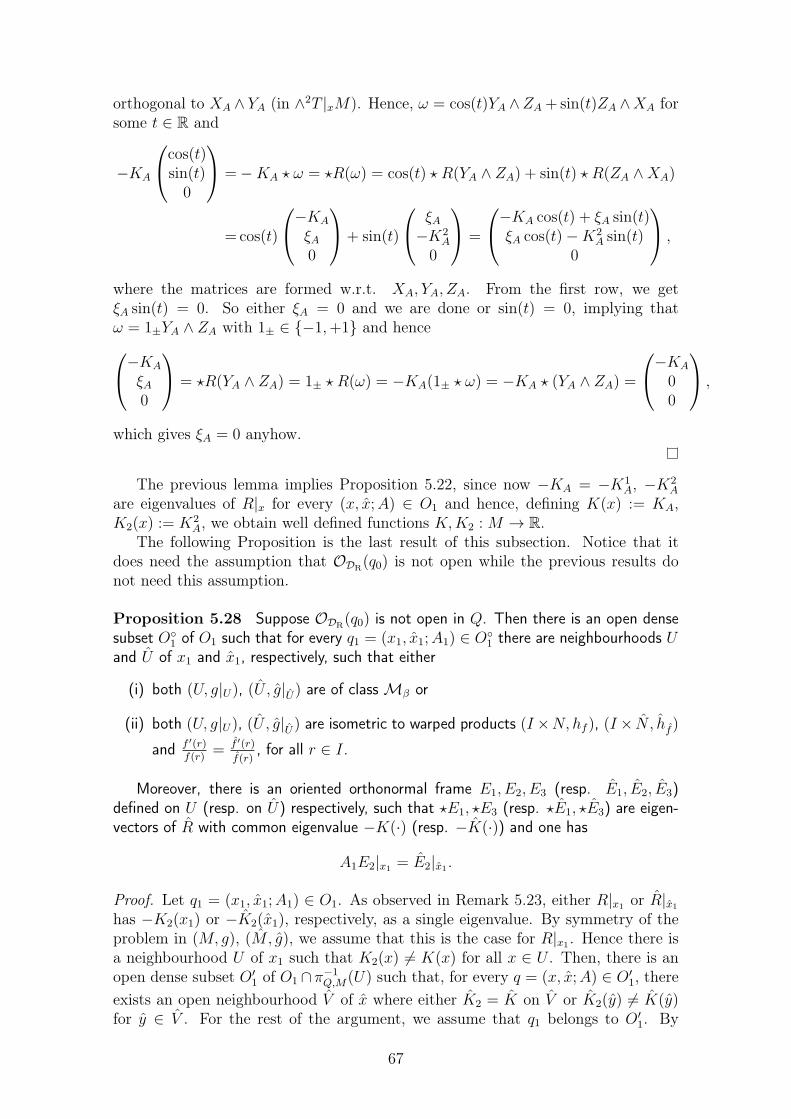
orthogonal to XA ∧ YA (in ∧2T |xM). Hence, ω = cos(t)YA ∧ZA + sin(t)ZA ∧XA forsome t ∈ R and

−KA

cos(t)sin(t)0

=−KA ⋆ ω = ⋆R(ω) = cos(t) ⋆ R(YA ∧ ZA) + sin(t) ⋆ R(ZA ∧XA)

= cos(t)

−KA

ξA0

+ sin(t)

ξA−K2

A

0

=

−KA cos(t) + ξA sin(t)ξA cos(t)−K2

A sin(t)0

,

where the matrices are formed w.r.t. XA, YA, ZA. From the first row, we getξA sin(t) = 0. So either ξA = 0 and we are done or sin(t) = 0, implying thatω = 1±YA ∧ ZA with 1± ∈ −1,+1 and hence−KA

ξA0

= ⋆R(YA ∧ ZA) = 1± ⋆ R(ω) = −KA(1± ⋆ ω) = −KA ⋆ (YA ∧ ZA) =

−KA

00

,

which gives ξA = 0 anyhow.

The previous lemma implies Proposition 5.22, since now −KA = −K1A, −K2

A

are eigenvalues of R|x for every (x, x;A) ∈ O1 and hence, defining K(x) := KA,K2(x) := K2

A, we obtain well defined functions K,K2 :M → R.The following Proposition is the last result of this subsection. Notice that it

does need the assumption that ODR(q0) is not open while the previous results do

not need this assumption.

Proposition 5.28 Suppose ODR(q0) is not open in Q. Then there is an open dense

subset O1 of O1 such that for every q1 = (x1, x1;A1) ∈ O

1 there are neighbourhoods Uand U of x1 and x1, respectively, such that either

(i) both (U, g|U), (U , g|U) are of class Mβ or

(ii) both (U, g|U), (U , g|U) are isometric to warped products (I ×N, hf ), (I × N , hf )

and f ′(r)f(r)

= f ′(r)

f(r), for all r ∈ I.

Moreover, there is an oriented orthonormal frame E1, E2, E3 (resp. E1, E2, E3)defined on U (resp. on U) respectively, such that ⋆E1, ⋆E3 (resp. ⋆E1, ⋆E3) are eigen-vectors of R with common eigenvalue −K(·) (resp. −K(·)) and one has

A1E2|x1 = E2|x1 .

Proof. Let q1 = (x1, x1;A1) ∈ O1. As observed in Remark 5.23, either R|x1 or R|x1

has −K2(x1) or −K2(x1), respectively, as a single eigenvalue. By symmetry of theproblem in (M, g), (M, g), we assume that this is the case for R|x1 . Hence there isa neighbourhood U of x1 such that K2(x) 6= K(x) for all x ∈ U . Then, there is anopen dense subset O′

1 of O1 ∩ π−1Q,M(U) such that, for every q = (x, x;A) ∈ O′

1, there

exists an open neighbourhood V of x where either K2 = K on V or K2(y) 6= K(y)for y ∈ V . For the rest of the argument, we assume that q1 belongs to O′

1. By

67

shrinking U around x1 and taking a small enough neighbourhood U of x1, weassume there are oriented orthonormal frames E1, E2, E3 on U (resp. E1, E2, E3

on U) such that ⋆E1, ⋆E2, ⋆E3 (resp. E1, E2, E3) are eigenvectors of R (resp. R)with eigenvalues −K(·),−K2(·),−K(·) (resp. −K(·),−K2(·),−K(·)), where theseeigenvalues correspond to those in Proposition 5.22. Taking U , U smaller if nec-essary, we take XA, YA, ZA as given by Proposition 5.22 for M and XA, YA, ZA forM on π−1

Q (U × U) ∩ O′1, which we still denote by O′

1. Since ⋆YA and ⋆E2|x areboth eigenvalues of R|x, for q = (x, x;A) ∈ O′

1, corresponding to single eigenvalue−K2(x), we moreover assume that YA = E2|x, ∀q = (x, x;A) ∈ O′

1. Then becauseν(Rolq(ZA ∧ XA))|q = −KRol

2 (q)ν(A ⋆ E2)|q is tangent to the orbit ODR(q0) at the

points q = (x, x;A) ∈ O′1, we conclude from Proposition 5.3 that

Γ =

Γ1(2,3) 0 −Γ1

(1,2)

Γ1(3,1) Γ2

(3,1) Γ3(3,1)

Γ1(1,2) 0 Γ1

(2,3)

,

where Γ and Γi(j,k) are as defined there.

We will now divide the proof in two parts (cases I and II below), dependingwhether (M, g) has, in certain areas, constant curvature or not.

Case I: Suppose, after shrinking U around x1, that K2(x) = K(x) for all x ∈U . We also assume that U is connected. This implies by Schur Lemma (see [30],Proposition II.3.6) that K2 = K is constant on U and we write simply K for thisconstant. Again by possibly shrinking U , we assume that (U , g|U) is isometric to anopen subset of a 3-sphere of curvature K.

Assume first that Γ1(2,3) 6= 0 on U . Then Proposition C.17, case (ii), implies

that Γ1(1,2) = 0 on U and (Γ1

(2,3))2 = K(x) is constant on U , which must be K.

Hence if β := Γ1(2,3), which is constant on U , then (U, g|U) is of class Mβ as is

(U , g|U) and we are done (recall that M−β = Mβ) i.e., this is case (i). On the otherhand, if Γ1

(2,3) = 0 on U , then we have that (U, g|U), after possibly shrinking U , isisometric, by some F , to a warped product (I×N, hf ) by Proposition C.17 case (iii).At the same time, the space of constant curvature (U , g|U), again after shrinkingU if necessary, can be presented, isometrically by certain F , as a warped product(I × N , hf ), where N is a 2-dimensional space of constant curvature. Because for

all x ∈ U we have K(x) = K, we get that for all (r, y) ∈ I ×N , r ∈ I,

−f ′′(r)

f(r)= K(F (r, y)) = K = −

f ′′(r)

f(r).

It is not hard to see that we may choose f such that f(0) = f(0) and f ′(0) = f ′(0),which then implies that f(r) = f(r), for all r ∈ I. This leads us to case (ii)

Case II: We assume here that K2(x) 6= K(x) for all x ∈ U . The same way asfor (M, g) above, this implies that YA = E2|x and that w.r.t. the frame E1, E2, E3,Proposition 5.3 yields

Γ =

Γ1(2,3) 0 −Γ1

(1,2)

Γ1(3,1) Γ2

(3,1) Γ3(3,1)

Γ1(1,2) 0 Γ1

(2,3)

,

68

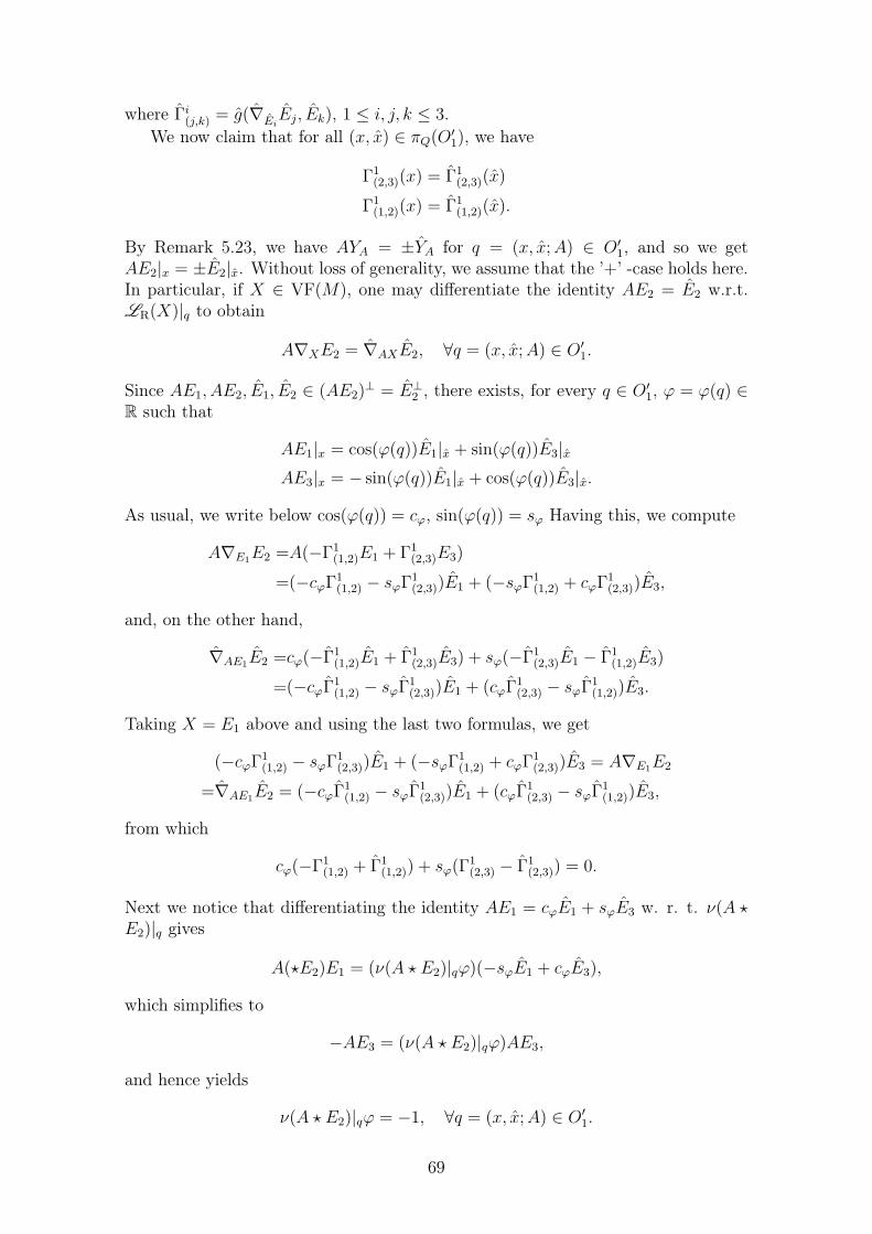
where Γi(j,k) = g(∇Ei

Ej, Ek), 1 ≤ i, j, k ≤ 3.We now claim that for all (x, x) ∈ πQ(O

′1), we have

Γ1(2,3)(x) = Γ1

(2,3)(x)

Γ1(1,2)(x) = Γ1

(1,2)(x).

By Remark 5.23, we have AYA = ±YA for q = (x, x;A) ∈ O′1, and so we get

AE2|x = ±E2|x. Without loss of generality, we assume that the ’+’ -case holds here.In particular, if X ∈ VF(M), one may differentiate the identity AE2 = E2 w.r.t.LR(X)|q to obtain

A∇XE2 = ∇AXE2, ∀q = (x, x;A) ∈ O′1.

Since AE1, AE2, E1, E2 ∈ (AE2)⊥ = E⊥

2 , there exists, for every q ∈ O′1, ϕ = ϕ(q) ∈

R such that

AE1|x = cos(ϕ(q))E1|x + sin(ϕ(q))E3|x

AE3|x = − sin(ϕ(q))E1|x + cos(ϕ(q))E3|x.

As usual, we write below cos(ϕ(q)) = cϕ, sin(ϕ(q)) = sϕ Having this, we compute

A∇E1E2 =A(−Γ1(1,2)E1 + Γ1

(2,3)E3)

=(−cϕΓ1(1,2) − sϕΓ

1(2,3))E1 + (−sϕΓ

1(1,2) + cϕΓ

1(2,3))E3,

and, on the other hand,

∇AE1E2 =cϕ(−Γ1(1,2)E1 + Γ1

(2,3)E3) + sϕ(−Γ1(2,3)E1 − Γ1

(1,2)E3)

=(−cϕΓ1(1,2) − sϕΓ

1(2,3))E1 + (cϕΓ

1(2,3) − sϕΓ

1(1,2))E3.

Taking X = E1 above and using the last two formulas, we get

(−cϕΓ1(1,2) − sϕΓ

1(2,3))E1 + (−sϕΓ

1(1,2) + cϕΓ

1(2,3))E3 = A∇E1E2

=∇AE1E2 = (−cϕΓ1(1,2) − sϕΓ

1(2,3))E1 + (cϕΓ

1(2,3) − sϕΓ

1(1,2))E3,

from which

cϕ(−Γ1(1,2) + Γ1

(1,2)) + sϕ(Γ1(2,3) − Γ1

(2,3)) = 0.

Next we notice that differentiating the identity AE1 = cϕE1 + sϕE3 w. r. t. ν(A ⋆E2)|q gives

A(⋆E2)E1 = (ν(A ⋆ E2)|qϕ)(−sϕE1 + cϕE3),

which simplifies to

−AE3 = (ν(A ⋆ E2)|qϕ)AE3,

and hence yields

ν(A ⋆ E2)|qϕ = −1, ∀q = (x, x;A) ∈ O′1.

69

Thus, if (t, q) 7→ Φ(t, q) is the flow of ν((·) ⋆ E2) in O′2 with initial position at t = 0

at q ∈ O′1, the above implies that ϕ(Φ(t, q)) = ϕ(q)+ t for all t such that |t| is small

enough. Since sin and cos are linearly independent functions on any non-empty openreal interval, the above relation implies that

−Γ1(1,2)(x) + Γ1

(1,2)(x) = 0,

Γ1(2,3)(x)− Γ1

(2,3)(x) = 0,

which establishes the claim.We may now finish the proof of the proposition. Indeed, if Γ1

(2,3) 6= 0 on U ,Proposition C.17 implies that Γ1

(2,3) =: β is constant and Γ1(1,2) = 0 on U . If x

belongs to the open subset πQ,M(O′1) of M , there is a q = (x, x;A) ∈ O′

1 where

(x, x) ∈ U × U , by the definition of O′1. The above implies

Γ1(1,2)(x) = Γ1

(1,2)(x) = 0, Γ1(2,3)(x) = Γ1

(2,3)(x) = β.

Thus shrinking U if necessary, this shows that Γ1(1,2) vanishes on U and Γ1

(2,3) is

constant = β on U . We conclude that (U, g|U) and (U , g|U) both belong to the classMβ and we are in case (i).

Similarly, if Γ1(2,3) = 0 on U , the above argument implies that, after taking smaller

U , that Γ1(2,3) = 0 on U . Proposition C.17 implies that there is, taking smaller U, U if

needed, open interval I = I ⊂ R, smooth functions f, f : I = I → R, 2-dimensionalRiemannian manifolds (N, h), (N , h) and isometries F : (I × N, hf ) → (U, g|U),F : (I × N , hf ) → U such that

f ′(r)

f(r)= Γ1

(1,2)(F (r, y)), ∀(r, y) ∈ I ×N,

f ′(r)

f(r)= Γ1

(1,2)(F (r, y)), ∀(r, y) ∈ I × N .

Clearly we may assume that 0 ∈ I = I and F (0, y1) = x1, F (0, y1) = x1 for somey1 ∈ N , y1 ∈ N . Since t 7→ (t, y1) and t 7→ (t, y1) are geodesics in (I × N, hf ),(I × N , hf ), respectively, γ(t) := F (t, y1) and γ(t) = F (t, y1) are geodesics on M

and M . In addition,

γ′(0) = E2|x1 = A1E2|x1 = A1γ′(0),

so γ(t) = γDR(γ, q1)(t) for all t. This means that

(F (t, y1), F (t, y1)) = (γ(t), γ(t)) ∈ πQ(O′1),

and therefore

f ′(t)

f(t)= Γ1

(1,2)(F (t, y1)) = Γ1(1,2)(F (t, y1)) =

f ′(t)

f(t),

for all t ∈ I = I. We then belong to case (ii) and the proof of the proposition isconcluded.

70

We have studied the case where q belongs to O1∪O2. As for the points of O0, oneuses Corollary 4.16 and Remark 4.17 to conclude that for every q0 = (x0, x0;A0) ∈O0, there are open neighbourhoods U ∋ x0 and U ∋ x0 such that (U, g|U) and(U , g|U) are locally isometric. With the choice of the set O as the union of O0 ∪O

1 ∪O2, (where O1 was introduced in Proposition 5.28), one concludes the proof of

Theorem 5.1.

5.3 Proof of Theorem 5.2

Only Items (b) and (c) are addressed and they are treated in separate subsections.

5.3.1 Case where both Manifolds are of Class Mβ

Consider two manifolds (M, g) and (M, g) of class Mβ, β ≥ 0 and oriented or-thonormal frames E1, E2, E3 and E1, E2, E3 which are adapted frames for of (M, g)and (M, g) respectively. We will prove that in this situation, the rolling problem isnot completely controllable.

We define on Q two subsets

Q0 :=q = (x, x;A) ∈ Q | AE2 6= ±E2,

Q1 :=q = (x, x;A) ∈ Q | AE2 = ±E2.

Proposition 5.29 Let (M, g), (M, g) be of class Mβ for β ∈ R. Then for anyq0 = (x0, x0;A0) ∈ Q1 one has ODR

(q0) ⊂ Q1. Moreover, Q1 is a closed 7-dimensionalsubmanifold of Q and hence in particular dimODR

(q0) ≤ 7.

Proof. Define h1, h2 : Q→ R by

h1(q) = g(AE1, E2), h2(q) = g(AE3, E2),

when q = (x, x;A) ∈ Q. Set h = (h1, h2) : Q→ R2, then Q1 = h−1(0). We will first

show that h is regular at the points of Q1, which then implies that Q1 is a closedsubmanifold of Q of codimension 2 i.e., dimQ1 = 7 as claimed. Before proceeding,we divide Q1 into two disjoint subsets

Q+1 =q = (x, x;A) ∈ Q | AE2 = +E2,

Q−1 =q = (x, x;A) ∈ Q | AE2 = −E2,

whence Q = Q+1 ∪Q−

1 . These are the components of Q and we prove the claims onlyfor Q+

1 , the considerations for Q−1 being completely similar. First, since for every

q = (x, x;A) ∈ Q+1 one has AE2 = E2, it follows that AE1, AE3 ∈ E⊥

2 and hencethere is a smooth φ : Q+

1 → R such that

AE1 = cos(φ)E1 + sin(φ)E3 =: XA,

AE3 = − sin(φ)E1 + cos(φ)E3 =: ZA.

In the sequel, we set cφ = cos(φ(q)), sφ = sin(φ(q)). For q = (x, x;A) ∈ Q+1 , one has

ν(A ⋆ E3)|qh1 = g(A(⋆E3)E1, E2) = g(AE2, E2) = 1,

ν(A ⋆ E1)|qh1 = g(A(⋆E1)E1, E2) = 0,

ν(A ⋆ E3)|qh2 = g(A(⋆E3)E3, E2) = 0,

ν(A ⋆ E1)|qh2 = g(A(⋆E1)E3, E2) = −g(AE2, E2) = −1,

71

which shows that indeed h is regular on Q+1 . We next show that the vectors

LR(E1)|q,LR(E2)|q,LR(E3)|q are all tangent to Q+1 and hence to Q1. This is equiv-

alent to the fact that LR(Ei)|qh = 0 for i = 1, 2, 3. We compute for q = (x, x;A) ∈

Q+1 , recalling that AE1 = XA, AE2 = ±E2, AE3 = ZA,

LR(E1)|qh1 =g(A∇E1E1, E2) + g(AE1, ∇XAE2)

=− Γ1(3,1)g(AE3, E2) + g(XA, βcφE3 − βsφE1)

=− Γ1(3,1)g(ZA, E2) + g(XA, βZA) = 0,

LR(E1)|qh2 =g(A∇E1E3, E2) + g(AE3, ∇XAE2)

=g(A(Γ1(3,1)E1 − βE2), E2) + g(ZA, βZA)

=g(Γ1(3,1)XA − βE2, E2) + β = 0,

LR(E2)|qh1 =g(A∇E2E1, E2) + g(AE1, ∇E2E2) = −Γ2

(3,1)g(ZA, E2) + 0 = 0,

LR(E2)|qh2 =g(A∇E2E3, E2) + g(AE3, ∇E2E2) = Γ2

(3,1)g(XA, E2) + 0 = 0,

LR(E3)|qh1 =g(A∇E3E1, E2) + g(AE1, ∇ZAE2)

=g(A(βE2 − Γ3(3,1)E3), E2) + g(XA,−βsφE3 − βcφE1)

=g(βE2 − Γ3(3,1)ZA), E2)− βg(XA, XA) = β − β = 0,

LR(E3)|qh2 =g(A∇E3E3, E2) + g(AE3, ∇ZAE2)

=Γ3(3,1)g(AE1, E2) + g(ZA,−βXA) = Γ3

(3,1)g(XA, E2) + 0 = 0.

Thus LR(E1)|q,LR(E2)|q,LR(E3)|q and hence DR are tangent to Q+1 , which implies

that any orbit ODR(q) through a point q ∈ Q+

1 , is also a subset of Q+1 . The same

observation obviously holds for Q−1 and therefore the proof is complete.

Next we will show that if (M, g) and (M, g) are of class Mβ with the sameβ ∈ R, then the rolling problem of M against M is not controllable. We beginby completing the proposition in the sense that we show that the orbit can be ofdimension exactly 7, if (M, g), (M, g) are not locally isometric.

Proposition 5.30 Let (M, g), (M, g) be Riemannian manifolds of class Mβ, β 6= 0,and let q0 = (x0, x0;A0) ∈ Q1. Then if ODR

(q0) is not an integral manifold of DR, onehas dimODR

(q0) = 7.

Proof. Without loss of generality, we assume that A0E2|x0 = E2|x0 . Then Proposi-tion 5.29 and continuity imply that AE2|x = E2|x for all q = (x, x;A) ∈ ODR

(q0)

and hence that AE1|x, AE3|x ∈ spanE1|x, E3|x. This combined with Lemma C.8implies

Rolq(⋆E1) = 0, Rolq(⋆E2) = (−K2(x) + K2(x))(⋆E2), Rolq(⋆E3) = 0,

for q = (x, x;A) ∈ ODR(q0), where −K2(x),−K2(x) are eigenvalues of R|x, R|x

corresponding to eigenvectors ⋆E2|x, ⋆E2|x, respectively. Since ODR(q0) is not an

integral manifold of DR, there is a point q1 = (x1, x1;A1) ∈ ODR(q0) such that

−K2(x1) + K2(x1) 6= 0 (see Corollary 4.16 and Remark 4.17). Then there areopen neighbourhoods U and U of x1 and x1 in M and M , respectively, such that−K2(x)+ K2(x) 6= 0 for all x ∈ U, x ∈ U . Define O := π−1

Q (U × U)∩ODR(q0), which

72

is an open subset of ODR(q0) containing q0. Because for all q = (x, x;A) ∈ O one

has ν(Rolq(⋆E2))|q ∈ T |qODR(q0) and −K2(x) + K2(x) 6= 0, it follows that

ν(A ⋆ E2)|q ∈ T |qODR(q0), ∀q = (x, x;A) ∈ O.

Moreover, Γ1(1,2) = 0 and Γ1

(2,3) = β is constant and hence one may use Proposition5.5, case (i), to conclude that the vector fields defined by

L1|q =LNS(E1)|q − βν(A ⋆ E1)|q,

L2|q =βLNS(E2)|q,

L3|q =LNS(E3)|q − βν(A ⋆ E2)|q,

are tangent to the orbit ODR(q0). Therefore the linearly independent vectors

LR(E1)|q,LR(E2)|q,LR(E3)|q, ν(A ⋆ E2)|q, L1|q, L2|q, L3|q,

are tangent to ODR(q0) for all q ∈ O, which implies that dimODR

(q0) ≥ 7. ByProposition 5.29, we conclude that dimODR

(q0) = 7.

We are left to study the case of an DR-orbit passing through some q0 ∈ Q0.

Proposition 5.31 Let (M, g) and (M, g) be two Riemannian manifolds of classMβ, β 6= 0, and let q0 = (x0, x0;A0) ∈ Q0. Write M := πQ,M(ODR

(q0)), M :=

πQ,M(ODR(q0)), which are open connected subsets of M , M . Then we have:

(i) If only one of (M, g) or (M, g) has constant curvature, then dimODR(q0) = 7.

(ii) Otherwise dimODR(q0) = 8.

Proof. As before, we let E1, E2, E3 and E1, E2, E3 to be some adapted frames of(M, g) and (M, g) respectively. We will not fix the choice of q0 in Q0 (and hencedo not define M, M) until the last half of the proof (where we introduce the setsM0,M1, M0, M1 below). Notice that Proposition 5.29 implies that ODR

(q0) ⊂ Q0,for every q0 ∈ Q0.

The fact that AE2|x 6= ±E2|x for q = (x, x;A) ∈ Q0 is equivalent to the fact thatthe intersection (AE⊥

2 |x) ∩ E⊥2 |x is non-trivial for all q = (x, x;A) ∈ Q0. Therefore,

for a small enough open neighbourhood O of q0 inside Q0, we may find a smoothfunctions θ, θ : O → R such that this intersection is spanned by AZA = ZA, where

ZA :=− sin(θ(q))E1|x + cos(θ(q))E3|x,

ZA :=− sin(θ(q))E1|x + cos(θ(q))E3|x.

We also define

XA := cos(θ(q))E1|x + sin(θ(q))E3|x,

XA := cos(θ(q))E1|x + sin(θ(q))E3|x.

To unburden the formulas, we set sτ := sin(τ(q)), cτ := cos(τ(q)) if τ : O → R issome function and the point q ∈ O is clear from the context. Since XA, E2|x, ZA

73

(resp. XA, E2|x, ZA) form an orthonormal frame for every q = (x, x;A) ∈ O andbecause A(Z⊥

A ) = Z⊥A , it follows that there is a smooth φ : O′ → R such that

AXA =cφXA + sφE2 = cφ(cθE1 + sθE3) + sφE2,

AE2 =− sφXA + cφE2 = −sφ(cθE1 + sθE3) + cφE2,

AZA =ZA.

In particular, for all q = (x, x;A) ∈ O, one has g(AZA, E2) = 0. Note that for allq = (x, x;A) ∈ O, since A ⋆ ZA = ⋆ZAA,

Rolq(⋆ZA) = R(⋆ZA)− AT R(⋆ZA)A = −K ⋆ ZA +KAT ⋆ZAA = 0,

and hence, since Rolq : ∧2T |xM → ∧2T |xM is a symmetric map,

Rolq(⋆XA) =−KRol

1 (q) ⋆ XA − α ⋆ E2,

Rolq(⋆E2) =− α ⋆ XA −KRol

2 (q) ⋆ E2,

for some smooth real-valued functions KRol

1 , KRol

2 , α defined on O.We begin by considering the smooth 5-dimensional distribution ∆ on the open

subset O of Q0 spanned by

LR(E1)|q,LR(E2)|q,LR(E3)|q, ν(A ⋆ E2)|q, ν(A ⋆ XA)|q.

What will be shown is that Lie(∆) spans at every point q ∈ O a smooth distri-bution Lie(∆)|q of dimension 8 which, by construction, is involutive. We considerVFk

DR,VFk

∆,Lie(∆) as C∞(O)-modules. Since XA = cθE1 + sθE3, in order to com-pute brackets of the first 4 vector fields above against ν(A⋆XA)|q, we need to knowsome derivatives of θ. We begin by computing the following.

LR(XA)|qZ(·) =(−LR(XA)|qθ + cθΓ1(3,1) + sθΓ

3(3,1))XA − βE2,

LR(E2)|qZ(·) =(−LR(E2)|qθ + Γ2(3,1))XA,

LR(ZA)|qZ(·) =(−LR(ZA)|qθ − sθΓ1(3,1) + cθΓ

3(3,1))XA.

Differentiating g(AZA, E2) = 0 with respect to LR(XA)|q gives,

0 =g(ALR(XA)|qZ(·), Y ) + g(AZA, ∇AXAE2)

=g(A(−LR(XA)|qθ + cθΓ1(3,1) + sθΓ

3(3,1))XA − βE2), E2)

+ g(AZA, cφcθβE3 − cφsθβE1)

=sφ(−LR(XA)|qθ + cθΓ1(3,1) + sθΓ

3(3,1))− βcφ + cφs

2θβ + cφc

2θβ


3(3,1)).

Since sφ 6= 0 (because otherwise AE2 = ±E2), we get


3(3,1).

In a similar way, differentiating g(AZA, E2) = 0 with respect to LR(ZA)|q, LR(E2)|q,one finds

LR(ZA)|qθ = −sθΓ1(3,1) + cθΓ

3(3,1),

LR(E2)|qθ = −β + Γ2(3,1).

74

and similarly, by using [LR(E3), ν((·) ⋆ E2)] = −LR(E1)|q + L1|q, one gets L1|qθ =Γ1(3,1). On the other hand, LNS(E2)|qZ(·) = (−LNS(E2)|qθ + Γ2

(3,1))XA, and to com-

pute L2|qθ = LNS(E2)|qθ, operate by LNS(E2)|q onto equation g(AZA, E2) = 0 toget L2|qθ = Γ2

(3,1). With these derivatives of θ being available, we easily see that

[L1, ν((·) ⋆ X(·))]|q =0,

[L1, L2]|q =(Γ2(3,1) + β)L3|q,

[L3, ν((·) ⋆ X(·))]|q =0,

[L3, L2]|q =− (Γ2(3,1) + β)L1|q,

[LR(E1), L2]|q =βL3|q − LR(∇E2E1)|q,

[LR(E2), L2]|q =0,

[LR(E3), L2]|q =− βL1|q − LR(∇E2E3)|q,

[ν((·) ⋆ E2), L2]|q =0,

[ν((·) ⋆ X(·)), L2]|q =0.

Hence we have proved that VF2∆ is involutive and hence

Lie(∆) = VF2∆.

There being 8 linearly independent generators for Lie(∆) = VF2∆, we conclude that

the distribution D spanned pointwise on O by Lie(∆) is integrable by Frobeniustheorem. The choice of q0 ∈ Q0 was arbitrary and we thus can build an 8-dimensionalsmooth involutive distribution D by the above construction on the whole Q0. SinceDR ⊂ ∆ ⊂ D, we have ODR

(q0) ⊂ OD(q0) for all q0 ∈ Q0 and thus dimODR(q0) ≤ 8.

We will show when the equality holds here and show when actually dimODR(q0) =

7. Define

M0 =x ∈M | β2 6= K2(x),

M1 =x ∈M | ∃ open V ∋ x s.t. ∀x′ ∈ V, β2 = K2(x′),

M0 =x ∈ M | β2 6= K2(x),

M1 =x ∈ M | ∃ open V ∋ x s.t. ∀x′ ∈ V , β2 = K2(x′),

and notice that M0∪M1 (resp. M0∪M1) is an open dense subset of M (resp. M). Atthis point we also fix q0 ∈ Q0 and write M = πQ,M(ODR

(q0)), M = πQ,M(ODR(q0))

as in the statement of this proposition. Let q1 = (x1, x1;A1) ∈ π−1Q (M0 × M0) ∩Q0.

Take an open neighbourhood O of q1 inQ0 as above (now for q1 instead of q0 which wefixed) such that πQ(O) ⊂M0 × M0, and introduce on O the vectors XA, ZA, XA, ZA

along with the angles θ, θ, φ, again as above. For q ∈ O, one has(Rolq(⋆XA)

Rolq(⋆E2)

)=

(s2φ(−β2 + K2) cφsφ(−β

2 + K2)

(−β2 + K2)sφcφ −K2 + s2φβ2 + c2

φK2

)(⋆XA

⋆E2

),

Rolq(⋆ZA) =0.

The determinant d(q) of the above matrix is equal to

d(q) = −s2φ(−K2 + β2)(−K2 + β2),

76

so d(q) 6= 0 since q ∈ O ⊂ π−1Q (M0 × M0) ∩ Q0. Since ν(Rol(⋆E2)(A))|q1 ∈

T |q1ODR(q1), we obtain that ν(A1 ⋆ E2)|q1 ∈ T |q1ODR

(q1). If q1 = (x1, x1;A1) ∈

π−1Q (M0 × M0) ∩ Q0, then one can take a sequence q′n = (x′n, x

′n;A

′n) ∈ ODR

(q1)

such that q′n → q1 while x′n ∈ M0. Since M0 and Q0 are open, we have for largeenough n that q′n ∈ π−1

Q (M0 × M0) ∩ Q0, hence ν(A′n ⋆ E2)|q′n ∈ T |q′nODR

(q1) andby taking the limit as n → ∞, we have ν(A1 ⋆ E2)|q1 ∈ T |q1ODR

(q1). Supposenext q1 = (x1, x1;A1) ∈ π−1

Q (M0 × M1) ∩ Q0. Then Rolq1(⋆E1) = Rolq1(⋆E3) = 0,

Rolq1(⋆E2) = (−K2(x1) + β2) ⋆ E2 with K2(x1) 6= β2 and hence ν(A ⋆ E2)|q1 ∈T |q1ODR

(q1). Thus we have proven that

ν(A ⋆ E2)|q ∈ T |qODR(q), ∀q ∈ Q0 ∩ π

−1Q (M0 × M).

Changing the roles of M and M we also have

ν((⋆E2)A)|q ∈ T |qODR(q), ∀q ∈ Q0 ∩ π

−1Q (M × M0).

On Q, define two 3-dimensional distributions D, D as follows, for q ∈ Q let D|qbe the span of

K1|q = LNS(AE1)|q + βν(A ⋆ E1)|q,

K2|q = LNS(AE2)|q,

K3|q = LNS(AE3)|q + βν(A ⋆ E3)|q,

and D|q be the span of

K1|q = LNS(AT E1)|q − βν((⋆E1)A)|q,

K2|q = LNS(AT E2)|q,

K3|q = LNS(AT E3)|q − βν((⋆E3)A)|q.

We claim that for any q1 = (x1, x1;A1) ∈ Q and any smooth paths γ : [0, 1] → M ,γ : [0, 1] → M with γ(0) = x1, γ(0) = x1 there are unique curves Γ, Γ : [0, 1] → Q ofthe same regularity as γ, γ such that Γ is tangent toD, Γ(0) = q1 and πQ,M(Γ(t)) = γ

and similarly Γ is tangent to D, Γ(0) = q1 and πQ,M(Γ(t)) = γ. The key point here

is that Γ, Γ are defined on [0, 1] and not only on a smaller interval [0, T ] with T ≤ 1.We write these curves as Γ = Γ(γ, q1) and Γ = Γ(γ, q1), respectively. Notice thatsince (πQ,M)∗D = 0 and (πQ,M)∗D = 0, one has

πQ,M(Γ(γ, q1)(t)) = x1, πQ,M(Γ(γ, q1)(t)) = x1, ∀t ∈ [0, 1].

We only prove the above claim for D since the proof for D is similar. Uniquenessand local existence are straigthforward. Take some extension of γ to an interval] − ǫ, 1 + ǫ[=: I and write Γ1 := Γ(γ, q1). Consider a trivialization (global since weassumed the frames Ei, Ei, i = 1, 2, 3 to be global) of πQ given by

Φ : Q→M × M × SO(n), (x, x;A) 7→ (x, x,MF,F (A)),

where F = (E1, E2, E3), F = (E1, E2, E3). For every (s, C) ∈ I × SO(n) one has

Φ(Γ(γ(s+ ·),Φ−1(γ(s), x1;C))(t)) = (γ(s+ t), x1, B(s,C)(t)),

77

where B(s,C)(t) ∈ SO(n) and t in an open interval containing 0. On I × SO(n),define a vector field

X|(s,C) := (∂

∂t, B(s,C)(0)).

If Φ(Γ(γ, q1)(t)) = (γ(t), x1;C1(t)), then since

d

dsΦ(Γ1(s)) =

d

dt

∣∣0Φ(Γ(γ, q1)(t+ s)) =

d

dt

∣∣0Φ(Γ(γ(s+ ·),Γ(γ, q1)(s))(t)

)

=d

dt

∣∣0(γ(t+ s), x1, B(s,C1(s))(t)) = (γ(s), 0, (pr2)∗X|(s,C1(s))),

we see that s 7→ (s, (pr3 Φ Γ1)(s)) = (s, C1(s)) is the integral curve of X startingfrom (0, C1(0)). Conversely, if Λ1(t) = (t, C(t)) is the integral curve of X startingfrom (0, C1(0)), then Γ1(t) := Φ−1(γ(t), x1, C(t)) gives an integral curve ofD startingfrom q1 and πQ,M(Γ1(t)) = γ(t).

Hence the maximal positive interval of definition of Γ1 is the same as that ofthe integral curve Λ1 of X starting from (0, C1). If it is of the form [0, t0[ for somet0 < 1 + ǫ, then, because [0, 1] × SO(n) is a compact subset of I × SO(n), there isa t1 ∈ [0, t0[ with Λ1(t1) /∈ [0, 1] × SO(n) i.e. t1 /∈ [0, 1] which is only possible ift1 > 1, and thus t0 > 1. We have shown that the existence of Γ1(t) = Γ(γ, q1)(t) isguaranteed on the whole interval [0, 1].

Since for all q ∈ Q0 ∩ π−1Q (M0 × M), which is an open subset of Q, one has

ν(A ⋆ E2)|q ∈ T |qODR(q), it follows from Proposition 5.5 that

L1|q = LNS(E1)|q − βν(A ⋆ E1)|q,

L2|q = LNS(E2)|q,

L3|q = LNS(E3)|q − βν(A ⋆ E3)|q,

are tangent to the orbit ODR(q) and hence so are LR(E1)|q−L1|q = K1|q, LR(E2)|q−

L2 = K2|q and LR(E3)|q − L3|q = K3|q i.e.,

D|q ⊂ T |qODR(q), ∀q ∈ Q0 ∩ π

−1Q (M0 × M).

A similar argument shows that

D|q ⊂ T |qODR(q), ∀q ∈ Q0 ∩ π

−1Q (M × M0).

Assume now that (M1 × M0) ∩ πQ(ODR(q0)) 6= ∅ and that M0 6= ∅. Choose

any q1 = (x1, x1;A1) ∈ ODR(q0) with (x1, x1) ∈ M1 × M0 and take any curve

γ : [0, 1] → M with γ(0) = x1, γ(1) ∈ M0. Then since πQ,M(Γ(γ, q1)(t)) = x1, we

have πQ(Γ(γ, q1)(t)) ∈ M × M0 for all t ∈ [0, 1] and since also D|q ⊂ T |qODR(q0)

for all q ∈ ODR(q0) ∩ π−1

Q (M × M0), we have that Γ(γ, q1)(t) ∈ ODR(q0) for all

t ∈ [0, 1]. Indeed, suppose there is a 0 ≤ t < 1 with Γ(γ, q1)(t) /∈ ODR(q0)

and define t1 = inft ∈ [0, 1] | Γ(γ, q1)(t) /∈ ODR(q0). Clearly t1 > 0. Be-

cause q2 := Γ(γ, q1)(t1) ∈ π−1Q (M × M0), it follows that for |t| small one has

Γ(γ, q1)(t1+t) ∈ ODR(q2), whence if t < 0 small, Γ(γ, q1)(t1+t) ∈ ODR

(q2)∩ODR(q0),

which means that q2 ∈ ODR(q0) and thus for t ≥ 0 small Γ(γ, q1)(t1+t) ∈ ODR

(q0), a

78

contradiction. Hence one has πQ(Γ(γ, q1)(1)) ∈ (M0 × M0) ∩ πQ(ODR(q0)). In other

words we have the implication:

(M1 × M0) ∩ πQ(ODR(q0)) 6= ∅, M0 6= ∅ =⇒ (M0 × M0) ∩ πQ(ODR

(q0)) 6= ∅.

By a similar argument, using D instead of D, one has that

(M0 × M1) ∩ πQ(ODR(q0)) 6= ∅, M0 6= ∅ =⇒ (M0 × M0) ∩ πQ(ODR

(q0)) 6= ∅.

Suppose now that there exists q1 = (x1, x1;A1) ∈ π−1Q (M0 × M0) ∩ ODR

(q0). Wealready know that T |q1ODR

(q0) contains vectors

LR(E1)|q1 ,LR(E2)|q1 ,LR(E3)|q1 ,

ν(A ⋆ E2)|q1 , ν((⋆E2)A)|q1 ,

L1|q1 , L2|q1 , L3|q1 ,

which are linearly independent since q1 ∈ (M0 × M0) ∩ πQ(ODR(q0)). Indeed, if one

introduces XA, ZA and an angle φ as before, we have sin(φ(q1)) 6= 0 as q1 ∈ Q0 and

ν((⋆E2)A1)|q1 = ν(A1 ⋆ (AT1 E2))|q1 = sin(φ(q1))ν(A1 ⋆ XA1)|q1 + cos(φ(q1))ν(A1 ⋆ E2)|q1 .

Therefore dimODR(q0) ≥ 8 and since we have also shown that dimODR

(q0) ≤ 8, wehave that

(M0 × M0) ∩ πQ(ODR(q0)) 6= ∅ =⇒ dimODR

(q0) = 8

Write Q := π−1Q (M×M), which is an open subset of Q and clearly ODR

(q0) ⊂Q. To finish the proof, we proceed case by case.

a) Suppose (M, g) has constant curvature i.e. M0∩M = ∅. By assumption then,

(M, g) does not have constant curvature, which means that M0 ∩M 6= ∅.

At every q = (x, x;A) ∈ Q, one has Rolq(⋆E1) = Rolq(⋆E3) = 0 andRolq(⋆E2) = (−K2(x) + β2) ⋆ E2 and therefore

[LR(E1),LR(E2)]|q = LR([E1, E2])|q, [LR(E2),LR(E3)]|q = LR([E2, E3])|q,

[LR(E3),LR(E1)]|q = LR([E3, E1])|q + (−K2(x) + β2)ν(A ⋆ E2)|q.

From these, Proposition 5.5 case (ii) and from the brackets (as above)

[LR(E1), L2]|q =βL3|q − LR(∇E2E1)|q,

[LR(E3), L2]|q =− βL1|q − LR(∇E2E3)|q,

[LR(E2), L2]|q =0,

[ν((·) ⋆ E2), L2]|q =0,

[L1, L2]|q =(Γ2(3,1) + β)L3|q,

[L3, L2]|q =− (Γ2(3,1) + β)L1|q,

we see that the distribution Don Q spanned by the 7 linearly independentvector fields

LR(E1),LR(E2),LR(E3), ν((·) ⋆ E2), L1, L2, L3,

79

with L1, L2, L3 as above, is involutive. Moreover D contains DR|Q , whichimplies ODR

(q0) = ODR|Q (q0) ⊂ OD(q0) and hence dimODR(q0) ≤ 7.

To show the equality here, notice that since M0 ∩ M 6= ∅, one has thatO := π−1

Q,M(M0)∩ODR(q0) is an open non-empty subset of ODR

(q0). Moreover,because K2(x) 6= β2 on M0 ∩M, we get that ν(A ⋆ E2)|q ∈ T |qODR

(q0) forall q ∈ O, from which one deduces by Proposition 5.5, case (i) that D|q ⊂T |qODR

(q0), which then implies dimODR(q0) ≥ 7. This proves one half of case

(i) in the statement of this proposition.

b) If (M, g) has constant curvature, one proves as in case a), by simply changingthe roles of M and M , that dimODR

(q0) = 7. This finishes the proof of case(i) of this proposition.

For the last case, we assume that neither (M, g) nor (M, g) have constantcurvature i.e. we have M ∩M0 6= ∅ and M ∩ M0 6= ∅.

c) Since M ∩M0 6= ∅, there is a q1 = (x1, x1;A1) ∈ ODR(q0) such that x1 ∈M0.

If x1 ∈ M0, we have (M0 × M0) ∩ πQ(ODR(q0)) 6= ∅ and which implies, as we

have shown, that dimODR(q0) = 8.

Suppose then that x1 ∈ M1. Then one may choose a sequence q′n = (x′n, x′n;A

′n) ∈

ODR(q0) such that q′n → q1 and x′n ∈ M1. Because M0 is open, for n large

enough one has (x′n, x′n) ∈ (M0 × M1) ∩ πQ(ODR

(q0)). Hence (M0 × M1) ∩

πQ(ODR(q0)) 6= ∅ and ∅ 6= M ∩ M0 ⊂ M0, which has been shown to imply

that (M0 × M0) ∩ πQ(ODR(q0)) 6= ∅ and again dimODR

(q0) = 8.

The proof is complete.

Remark 5.32 One could adapt the proofs of Propositions 5.29, 5.30 and 5.31 to dealalso with the case β = 0. For example, Proposition 5.29 as formulated already is validin this case, but the conclusion when β = 0 could be strengthened to dimODR

(q0) ≤ 6.However, since a Riemannian manifold of class M0 is also locally a Riemannian product,and hence locally a warped product, we prefer to view this special case β = 0 as part ofthe subject of Subsection 5.3.2.

5.3.2 Case where both manifolds are Warped Products

Suppose (M, g) = (I × N, hf ) and (M, g) = (I × N , hf ), where I, I ⊂ R are open

intervals, (N, h) and (N , h) are connected, oriented 2-dimensional Riemannian man-ifolds and the warping functions f, f are smooth and positive everywhere. We write∂∂r

for the canonical, positively directed unit vector field on (R, s1) and consider itas a vector field on (M, g) and (M, g) as is usual in direct products. Notice thatthen ∂

∂ris a g-unit (resp. g-unit) vector field on M (resp. M) which is orthogonal

to T |yN (resp. T |yN) for every (r, y) ∈ M (resp. (r, y) ∈ N). We will prove thatstarting from any point point q0 ∈ Q = Q(M, M) and if the warping functions f, fsatisfy extra conditions relative to each other, then the orbit ODR

(q0) is either 6- or8-dimensional. The first case is formulated in the following proposition.

80

Proposition 5.33 Let (M, g) = (I × N, hf ), (M, g) = (I × N , hf ) be warped

products of dimension 3, with I, I ⊂ R open intervals. Also, let q0 = (x0, x0;A0) ∈ Qbe such that if one writes x0 = (r0, y0), x0 = (r0, y0), then

A0∂

∂r

∣∣(r0,y0)

=∂

∂r

∣∣(r0,y0)

. (50)

holds and

f ′(t+ r0)

f(t+ r0)=f ′(t+ r0)

f(t+ r0), ∀t ∈ (I − r0) ∩ (I − r0). (51)

Then if ODR(q0) is not an integral manifold of DR, one has dimODR

(q0) = 6.

Proof. For convenience we write κ(r) := f ′(r+r0)f(r+r0)

= f ′(r+r0)

f(r+r0), r ∈ (I−r0)∩(I−r0) =: J .

Let γ be a smooth curve in M defined on some interval containing 0 and such thatγ(0) = x0 and let (γ(t), γ(t);A(t)) = qDR

(γ, q0)(t) be the rolling curve generated byγ starting at q0 and defined on some (possible smaller) maximal interval containing0. Write γ(t) = (r(t), γ1(t)) and γ(t) = (r(t), γ1(t)) corresponding to the directproducts M = I ×N and M = I × N . Define also,

ζ(t) := r(t)− r0, S(t) :=∂

∂r

∣∣γ(t),

ζ(t) := r(t)− r0, S(t) :=A(t)−1 ∂

∂r

∣∣γ(t),

which are vector fields on M along γ. Notice that

ζ(t) = r(t) =g(γ(t),

∂

∂r

∣∣γ(t)

)= g(γ(t), S(t)),

˙ζ(t) = ˙r(t) =g

(˙γ(t),

∂

∂r

∣∣γ(t)

)= g(A(t)γ(t),

∂

∂r

∣∣γ(t)

)= g(γ(t), S(t)).

By Proposition 35, Chapter 7, p. 206 in [26], we have

∇γ(t)∂

∂r=f ′(r(t))

f(r(t))

(γ(t)− r(t)

∂

∂r

∣∣γ(t)

),

=κ(ζ(t))(γ(t)− ζ(t)

∂

∂r

∣∣γ(t)

),

∇ ˙γ(t)

∂

∂r=f ′(r(t))

f(r(t))

(˙γ(t)− ˙r(t)

∂

∂r

∣∣γ(t)

),

=κ(ζ(t))(˙γ(t)−

˙ζ(t)

∂

∂r

∣∣γ(t)

),

i.e.,

∇γ(t)S(t) =κ(ζ(t))(γ(t)− ζ(t)S(t)),

∇γ(t)S(t) =A(t)−1∇ ˙γ(t)

∂

∂r= κ(ζ(t))

(A(t)−1 ˙γ(t)−

˙ζ(t)A(t)−1 ∂

∂r

∣∣γ(t)

),

=κ(ζ(t))(γ(t)−˙ζ(t)S(t)).

81

Let ρ ∈ C∞(R) and t 7→ X(t) be a vector field along γ and consider a first orderODE

ρ(t) = g(γ(t), X(t)),

∇γ(t)X = κ(ρ(t))(γ(t)− ρ(t)X(t)).

By the above we see that the pairs (ρ,X) = (ζ, S) and (ρ,X) = (ζ , S) both solve thisODE. Moreover, by assumption ζ(0) = 0 = ζ(0) and S(0) = A(0)−1 ∂

∂r

∣∣x0

= ∂∂r

∣∣x0

=

S(0) so these pairs have the same initial conditions and hence (ζ, S) = (ζ , S) on theinterval where they are both defined. Then,

r(t)− r0 =r(t)− r0,

A(t)∂

∂r

∣∣γ(t)

=∂

∂r

∣∣γ(t),

for all t in the interval where the rolling curve qDR(γ, q0) is defined. Define

Q∗+ =

q = (x, x;A) = ((r, y), (r, y);A) ∈ Q | r − r0 = r − r0, A

∂

∂r

∣∣x=

∂

∂r

∣∣x

.

By the above considerations, as long as the curve is defined,

qDR(γ, q0)(t) ∈ Q∗

+,

which implies that ODR(q0) ⊂ Q∗

+. We show that Q∗+ is a 6-dimensional submanifold

of Q. Let q = (x, x;A) = ((r, y), (r, y);A) ∈ Q such that A ∂∂r

∣∣x= ∂

∂r

∣∣x. Then for all

α ∈ R, X ′ ∈ T |yN one has

‖X ′‖2g + α2 =

∥∥∥∥X ′ + α∂

∂r

∣∣x

∥∥∥∥2

g

=

∥∥∥∥A(X ′ + α∂

∂r

∣∣x)

∥∥∥∥2

g

= ‖AX ′‖2g + 2g

(AX ′, α

∂

∂r

∣∣x

)+ α2.

This implies that

‖X ′‖2g = ‖AX ′‖

2g ,

g(AX ′,

∂

∂r

∣∣x

)= 0,

for all X ′ ∈ T |yN . Thus AT |yN ⊥ ∂∂r

∣∣x

and also A ∂∂r

∣∣x⊥ T |yN by assumption.

Define

Q+1 =

q = (x, x;A) = ((r, y), (r, y);A) ∈ Q | A

∂

∂r

∣∣x=

∂

∂r

∣∣x

,

and let q1 = (x1, x1;A1) = ((r1, y1), (r1, y1);A1) ∈ Q+1 . Choose a local oriented h-

and h-orthonormal frames X ′1, X

′2 in N around y1 and X ′

1, X′2 in N around y1. Let

the corresponding domains be U ′ and U ′. Writing E1 =∂∂r

, E2 =1fX ′

1, E3 =1fX ′

2 on

M and E1 =∂∂r

, E2 =1

fX ′

1, E3 =1

fX ′

2 on M , we see that E1, E2, E3 and E1, E2, E3

are g- and g-orthonormal oriented frames and we define

Ψ : V := π−1Q ((R× U ′)× (R× U ′)) → SO(3),

Ψ(x, x;A) = [(g(AEi, Ej))ji ].

82

This is a chart of Q and clearly

Ψ(V ∩Q+1 ) = (R× U ′)× (R× U ′)×

(1 00 A′

)| A′ ∈ SO(2)

.

This shows that Q+1 ∩V is a 7-dimensional submanifold of Q and hence Q+

1 is a closed7-dimensional submanifold of Q. Defining F : Q+

1 → R by F ((r, y), (r, y);A) =(r− r0)− (r− r0), we see that Q∗

+ = F−1(0). Once we show that F is a submersion,it follows thatQ∗

+ is a closed codimension 1 submanifold ofQ+1 (i.e. dimQ∗

+ = 7−1 =6) and thus it is a 6-dimensional submanifold of Q. Indeed, let q = (x, x;A) ∈ Q+

1

and let γ(t) be an integral curve of ∂∂r

starting from x and γ(t) = x a constantpath. Let q(t) = (γ(t), γ(t);A(t)) be the DNS-lift of (γ, γ) starting from q. Thenγ(t) = ∂

∂r

∣∣γ(t)

, ˙γ(t) = 0 and since ∂∂r

is a unit geodesic field on M , one has

d

dtg(A(t)

∂

∂r

∣∣γ(t),∂

∂r

∣∣γ(t)

)= g(A(t)∇γ(t)

∂

∂r,∂

∂r

∣∣γ(t)

)+ g(A(t)

∂

∂r, ∇0

∂

∂r

∣∣γ(t)

)= 0.

This shows that q(t) ∈ Q+1 for all t and in particular, LNS(

∂∂r

∣∣x)|q = q(0) ∈ T |qQ

+1 .

Then if one writes γ(t) = (r(t), γ1(t)), γ(t) = x = (r, y)=constant, one has r(t) = 1and therefore

d

dt

∣∣0F (q(t)) =

d

dt

∣∣0

((r(t)− r0)− (r − r0)

)= 1,

i.e., F∗LNS(∂∂r

∣∣x)|q = 1, which shows that F is submersive. (Alternatively, one

could have uses the charts Ψ as above to prove this fact.) Since we have shownthat dimQ∗

+ = 6 and ODR(q0) ⊂ Q∗

+, it follows that ODR(q0) ≤ 6. To prove the

equality here, we will use the assumption that ODR(q0) is not an integral manifold

of DR. Take local frames Ei, Ei as above near x1 and x1, where q1 = (x1, x1;A1) =

((r1, y1), (r1, y1);A1) ∈ ODR(q0). The assumption that f ′(t+r0)

f(t+r0)= f ′(t+r0)

f(t+r0)for all t ∈ J

easily imply that f ′′(t+r0)f(t+r0)

= f ′′(t+r0)

f(t+r0)=: κ2(t) for all t ∈ J as well. Respect to the

frames ⋆E1, ⋆E2, ⋆E3 and ⋆E1, ⋆E2, ⋆E3 one has (see Proposition 42, Chapter 7, p.210 of [26])

R|(r,y) =

− σ(y)

f(r)2+ κ(r − r0)

2 0 0

0 κ2(r − r0) 00 0 κ2(r − r0)

,

R|(r,y) =

− σ(y)

f(r)2+ κ(r − r0)

2 0 0

0 κ2(r − r0) 00 0 κ2(r − r0)

,

where σ(y) and σ(y) are the unique sectional curvatures of (N, h) and (N , h) atpoints y, y. Write

−K2(r, y) = −σ(y)

f(r)2+ κ(r − r0), −K2(r, y) = −

σ(y)

f(r)2+ κ(r − r0).

Since A1∂∂r

∣∣x1

= ∂∂r

∣∣x1

, we already know that A1E2|x1 and A1E3|x1 are in the plane

spanE2|x1 , E3|x1. This and the fact that r1 − r0 = r1 − r0 imply that

Rolq1 =

−K2(x1) + K2(x1) 0 0

0 0 00 0 0

,

83

w.r.t. ⋆E1|x1 , ⋆E2|x1 , ⋆E3|x1 . Since ODR(q0) is not an integral manifold of DR, it

follows from Corollary 4.16 and Remark 4.17 that there is a q1 ∈ ODR(q0), where

Rolq1 6= 0. Hence there is a neighbourhood O of q1 in ODR(q0) such that Rolq 6= 0.

With respect to local frames Ei, Ei as above (taking O smaller if necessary), thismeans that K2(x) 6= K2(x) for all q = (x, x;A) ∈ O and since ν(Rolq(⋆E1))|q =

(−K2(x) + K2(x))ν(A ⋆ E1)|q, we have

ν(A ⋆ E1)|q ∈ T |qODR(q0), ∀q ∈ O.

Hence applying Proposition 5.5 case (i) to the frame F1 := E2, F2 := E1, F3 := E3

implies that the 6 linearly independent vectors (notice that we have Γ1(2,3) = 0 in

that proposition)

LR(F1)|q,LR(F2)|q,LR(F3)|q, ν(A ⋆ F2)|q, L1|q, L3|q,

are tangent to ODR(q0) at q ∈ O, where

L1 = LNS(F1)|q − Γ1(1,2)(x)ν(A ⋆ F3)|q,

L3 = LNS(F3)|q + Γ1(1,2)(x)ν(A ⋆ F1)|q,

with Γ1(1,2)(x) = g(∇F1F1F2) = g(∇E2E2, E1) = −f ′(r)

f(r)if x = (r, y). Hence dimODR

(q0) ≥6.

Remark 5.34 The condition Rolq1 6= 0 in the proof of the previous proposition was

equivalent to the condition K2(x1) 6= K2(x1) which again means that if x1 = (r1, y1),x1 = (x1, y1),

σ(y1)

f(r1)26=

σ(y1)

f(r1)2,

where σ(y) (resp. σ(y)) is the sectional curvature of (N, h) at y ∈ N (resp. of (N , h)at y ∈ N).

Remark 5.35 To show that dimODR(q0) ≤ 6 under the assumptions of the propo-

sition, we showed that if q = (x, x;A) ∈ Q∗+, then qDR

(γ, q)(t) ∈ Q∗+ for any path

γ starting from x. For this we basically used the uniqueness of the solutions of anODE. Alternatively, one could have proceeded exactly in the same way as in the proof ofProposition 5.29. To this end, one defines as there h1, h1 : Q→ R and also F : Q→ R

as above as

h1(q) = g(AE1, E2), h2(q) = g(AE3, E2), F (q) = (r − r0)− (r − r0).

Write H = (h1, h2, F ) : Q → R3, Q∗ := H−1(0) and Q = Q∗

+ ∪ Q∗− where Q∗

+ (resp.Q∗

−) consists of all q = (x, x;A) ∈ Q∗ where A ∂∂r

= + ∂∂r

(resp. A ∂∂r

= − ∂∂r

). Then,for all q ∈ Q∗

+,

H∗ν(A ⋆ E1)|q = (0,−1, 0), H∗ν(A ⋆ E3)|q = (1, 0, 0), H∗LNS(∂

∂r, 0)|q = (0, 0, 1),

84

which shows (again) that Q∗+ is a 6-dimensional closed submanifold of Q (and so is Q∗)

while w.r.t. orthonormal bases E1, E2, E3, E1, E2, E3, where E2 = ∂∂r

, E2 = ∂∂r

, onehas for q = (x, x;A) ∈ Q∗

+, since x = (r, y), x = (r, y) with r − r0 = r − r0 =: t,

LR(E1)|qh1 = g(A(Γ1(1,2)E2 − Γ1

(3,1)E3), E2) + g(AE1,−Γ1(1,2)AE1)

= −f ′(r)

f(r)+f ′(r)

f(r)= −

f ′(t+ r0)

f(t+ r0)+f ′(t+ r0)

f(t+ r0)= 0,

LR(E1)|qh2 = Γ1(3,1)g(AE1, E2) + g(AE3,−Γ1

(1,2)AE1) = 0,

LR(E2)|qh1 = −Γ2(3,1)g(AE3, E2) = 0,

LR(E2)|qh2 = Γ2(3,1)g(AE1, E2) = 0,

LR(E3)|qh1 = LR(E3)|qh2 = 0,

LR(E1)|qF = LR(E2)|qF = LR(E3)|qF = 0,

hence DR|q ⊂ T |qQ∗+ for all q ∈ Q∗

+. This obviously implies that ODR(q) ⊂ Q∗

+ for allq ∈ Q∗

+ and thus dimODR(q) ≤ dimQ∗

+ = 6.

For the following proposition we introduce some more notations,

Q0 :=q = ((r, y), (r, y);A) ∈ Q | A∂

∂r

∣∣(r,y)

6= ±∂

∂r

∣∣(r,y)

,

Q+1 :=Q\Q0 = q = (x, x;A) ∈ Q | A

∂

∂r

∣∣(r,y)

= +∂

∂r

∣∣(r,y)

,

Q−1 :=Q\Q0 = q = (x, x;A) ∈ Q | A

∂

∂r

∣∣(r,y)

= −∂

∂r

∣∣(r,y)

,

Q1 :=Q+1 ∪Q−

1 ,

S+1 :=

q = ((r, y), (r, y);A) ∈ Q+

1 |f ′(r)

f(r)= +

f ′(r)

f(r)

,

S−1 :=

q = ((r, y), (r, y);A) ∈ Q−

1 |f ′(r)

f(r)= −

f ′(r)

f(r)

,

S1 :=S+1 ∪ S−

1 .

We have that Q decomposes into the disjoint union

Q = S1 ∪ (Q\S1) = S1 ∪ (Q1\S1) ∪Q0.

Proposition 5.36 Let (M, g) = (I × N, hf ) and (M, g) = (I × N , hf ), be warped

products with I, I ⊂ R open intervals and suppose that there is a constant K ∈ R suchthat

f ′′(r)

f(r)= −K =

f ′′(r)

f(r), ∀(r, r) ∈ I × I .

Let q0 = (x0, x0;A0) ∈ Q and write M := πQ,M(ODR(q0)), M

:= πQ,M(ODR(q0)).

Assuming that ODR(q0) is not an integral manifold of DR, we have the following cases:

(i) If q0 ∈ S1, then dimODR(q0) = 6;

85

(ii) If q0 ∈ Q\S1 and if only one of (M, g) or (M, g) has constant curvature, thendimODR

(q0) = 6;

(iii) Otherwise dimODR(q0) = 8.

Proof. As in the proof of Proposition 5.33 (see also Remark 5.35) it is clear thatQ1 is a closed 7-dimensional closed submanifolds of Q and Q−

1 , Q+1 are disjoint open

and closed submanifolds of Q1. Also, S1, S+1 , S

−1 are closed subsets of Q1. Let us

begin with the case where q0 ∈ S+1 . Writing x0 = (r0, y0), x0 = (r0, y0) and defining

w(t) := f ′(t+r0)f(t+r0)

− f ′(t+r0)

f(t+r0), we see that for all t ∈ (I − r0) ∩ (I − r0),

w′(t) =f ′′(t+ r0)

f(t+ r0)︸︷︷︸=−K

−(f ′(t+ r0)

f(t+ r0)

)2−f ′′(t+ r0)

f(t+ r0)︸︷︷︸=−K

+( f ′(t+ r0)

f(t+ r0)

)2,

i.e.,

w′(t) = −w(t)(f ′(t+ r0)

f(t+ r0)+f ′(t+ r0)

f(t+ r0)

), w(0) = 0.

This shows that w(t) = 0 for all t ∈ (I − r0) ∩ (I − r0) and hence the assumptionsof Proposition 5.33 have been met. Thus dimODR

(q0) = 6. On the other hand,if q0 = (x0, x0;A0) ∈ S−

1 and x0 = (r0, y0), x0 = (r0, y0), define f∨(t) := f(−t),I∨ := −I and notice that ϕ : (I × N , hf ) → (I∨ × N , hf∨) =: (M∨, g∨) given by

(y, r) 7→ (y,−r) is an isometry, which induces a diffeomorphism Φ : Q→ Q(M, M∨)by (x, x;A) 7→ (x, ϕ(x);ϕ∗|x A) which preserves the respective rolling distribu-tions and orbits: Φ∗(DR|q) = D∨

R|Φ(q), Φ(ODR(q)) = OD∨

R(Φ(q)), the notation being

clear here. But now Φ(A0) = ϕ∗(A0∂∂r) = −ϕ∗

∂∂r

= ∂∂r

and since q∨0 := Φ(q0) =((r0, y0), (−r0, y0);ϕ∗ A0),

(f∨)′(−r0)

f∨(−r0)=

ddt

∣∣0f∨(t− r0)

f(r0)=

ddt

∣∣0f(r0 − t)

f(r0)= −

f ′(r0)

f(r0)=f ′(r0)

f(r0).

Thus Φ(q0) belongs to the set S+1 of Q(M, M∨) (which corresponds by Φ to S−

1

of Q) and thus the above argument implies that dimOD∨

R(Φ(q0)) = 6 and there-

fore ODR(q0) = 6. Hence we have proven (i). We next deal with the case where

q0 ∈ Q\S1. Up until the second half of the proof, where we introduce the setsM0,M1, M0, M1, we assume that the choice of q0 ∈ Q\S1 is not fixed (and henceM, M are not defined yet). So let q0 = (x0, x0;A0) = ((r0, y0), (r0, y0);A0) ∈ Q\S1

and choose some orthonormal frame X1, X3 (resp. X1, X3) on N (resp. N) definedon an open neighbourhood U ′ of y0 (resp. U ′ of y0) and consider them, in the nat-ural way, as vector fields on M (resp. M). Moreover, assume that X1,

∂∂r, X3 (resp.

X1,∂∂r, X3) is oriented. Writing E1 = 1

fX1, E2 = ∂

∂r, E3 = 1

fX3, and E1 = 1

fX1,

E2 = ∂∂r

, E3 = 1

fX3, we get positively oriented orthonormal frames of M and M ,

defined on U := I×U ′, U := I× U ′, respectively. Then we have, by [26], Chapter 7,Proposition 42 (one should pay attention that there the definition of the curvature

86

tensor differs by sign to the definition used here) that with respect to the frames⋆E1, ⋆E2, ⋆E3 and ⋆E1, ⋆E2, ⋆E3,

R =

−K 0 0

0 −σ+(f ′)2

f2 0

0 0 −K

, R =

−K 0 0

0 −σ+(f ′)2

f20

0 0 −K

,

where σ(y) and σ(y) are the unique sectional (or Gaussian) curvatures of (N, h) and

(N , h) at points y, y. Write −K2 :=−σ+(f ′)2

f2 and −K2 :=−σ+(f ′)2

f2. We now take an

open neighbourhood O of q0 in Q according to the following cases:

(a) If q0 ∈ Q0, we assume that O ⊂ Q0 ∩ π−1Q (U × U).

(b) If q0 ∈ Q+1 \S1 (resp. q0 ∈ Q−

1 \S1) we assume that O ⊂ π−1Q (U × U)\(S1 ∪Q

−1 )

(resp. O ⊂ π−1Q (U × U)\(S1 ∪Q

+1 )).

Write O0 := O∩Q0. Thus in case (a) one has O = O0 ∋ q0 while in case (b) one hasO = O0∪(O∩(Q±

1 \S1)), as a disjoint union, and q0 /∈ O0, the "±" depending on therespective situation. Moreover, if the case (b) occurs, we assume that q0 ∈ Q+

1 \S1

since the case where q0 ∈ Q−1 \S1 is handled in a similar way. We will still shrink

O around q0 whenever convenient and always keep in mind that O0 = O ∩Q0 evenafter the shrinking. Notice that this shrinking does not change the properties in (a)and (b) above. Moreover, [26], Chapter 7, Proposition 35 implies that if Γ, Γ areconnection tables w.r.t. E1, E2, E3 and E1, E2, E3, respectively,

Γ =

0 0 −Γ1(1,2)

Γ1(3,1) Γ2

(3,1) Γ3(3,1)

Γ1(1,2) 0 0

, Γ =

0 0 −Γ1(1,2)

Γ1(3,1) Γ2

(3,1) Γ3(3,1)

Γ1(1,2) 0 0

,

and

W (Γ1(1,2)) =0, ∀W ∈ E⊥

2 ,

W (Γ1(1,2)) =0, ∀W ∈ E⊥

2 ,

since Γ1(1,2)(r, y) = −f ′(r)

f(r)and Γ1

(1,2)(r, y) = − f ′(r)

f(r). Actually one even has Γ2

(3,1) = 0

and Γ2(3,1) = 0, but we do not use this fact; one could for example rotate E1, E3

(resp. E1, E3) between them, in a non-constant way, to destroy this property. Thefact that AE2|x 6= ±E2|x for q = (x, x;A) ∈ Q0 is equivalent to the fact that theintersection (AE⊥

2 |x) ∩ E⊥2 |x is non-trivial for all q = (x, x;A) ∈ Q0. Therefore, by

shrinking O around q0 if necessary, we may find a smooth functions θ, θ : O0 → R

such that this intersection is spanned by AZA = ZA, where

ZA :=− sin(θ(q))E1|x + cos(θ(q))E3|x,

ZA :=− sin(θ(q))E1|x + cos(θ(q))E3|x.

We also define

XA := cos(θ(q))E1|x + sin(θ(q))E3|x,

XA := cos(θ(q))E1|x + sin(θ(q))E3|x.

87

To unburden the formulas, we write from now on usually sτ := sin(τ(q)), cτ :=cos(τ(q)) if τ : V → R is some function, V ⊂ Q, and the point q ∈ V is clear fromthe context. Since XA, E2|x, ZA (resp. XA, E2|x, ZA) form an orthonormal frame forevery q = (x, x;A) ∈ O0 and because A(Z⊥

A ) = Z⊥A , it follows that there is a smooth

φ : O0 → R such that

AXA =cφXA + sφE2 = cφ(cθE1 + sθE3) + sφE2,

AE2 =− sφXA + cφE2 = −sφ(cθE1 + sθE3) + cφE2,

AZA =ZA.

In particular, for all q = (x, x;A) ∈ O0, one has g(AZA, E2) = 0. Formulas in Eq.(45) on page 58 hold with Γ1

(2,3) = 0 and Y = E2. Since they are very useful incomputations, we will now derive three relations, two of which simplify Eq. (45),and all of which play an important role later on in the proof. Differentiating theidentity g(AZA, E2) = 0 with respect to LR(XA)|q, LR(E2)|q and LR(ZA)|q, one ata time, yields on O0,

0 =g(ALR(XA)Z(·), E2) + g(AZA, ∇AXAE2)

=(−LR(XA)|qθ + cθΓ1(3,1) + sθΓ

3(3,1))g(AXA, E2) + g(ZA,−cφΓ

1(1,2)XA)


3(3,1)),

0 =g(ALR(E2)Z(·), E2) + g(AZA, ∇AE2E2)

=(−LR(Y )|qθ + Γ2(3,1))g(AXA, E2) + g(ZA, sφΓ

1(1,2)XA)

=sθ(−LR(Y )|qθ + Γ2(3,1)),

0 =g(ALR(ZA)Z(·), E2) + g(AZA, ∇AZAE2)

=(−LR(ZA)|qθ − sθΓ1(3,1) + cθΓ

3(3,1))g(AXA, E2)

+ Γ1(1,2)g(AE2, E2) + g(ZA,−Γ1

(1,2)ZA)

=sφ(−LR(ZA)|qθ − sθΓ1(3,1) + cθΓ

3(3,1)) + cφΓ

1(1,2) − Γ1

(1,2).

Define

λ(q) := LR(ZA)|qθ + sθΓ1(3,1) − cθΓ

3(3,1), q ∈ O0,

which is a smooth function on O0. Since sin(φ(q)) = 0 would imply that AE2 = ±E2,we have sin(φ(q)) 6= 0 on O0 ⊂ Q0 and hence we get


3(3,1),

LR(E2)|qθ = Γ2(3,1),

sφλ = cφΓ1(1,2) − Γ1

(1,2).

These formulas, along with Γ1(2,3) = 0, simplify Eq. (45) to

LR(XA)|qX(·) = Γ1(1,2)E2, LR(E2)|qX(·) = 0, LR(ZA)|qX(·) = λZA,

LR(XA)|qE2 = −Γ1(1,2)XA, LR(E2)|qE2 = 0, LR(ZA)|qE2 = −Γ1

(1,2)ZA,

LR(XA)|qZ(·) = 0, LR(E2)|qZ(·) = 0, LR(ZA)|qZ(·) = −λXA + Γ1(1,2)E2, (52)

88

at q ∈ O0. We use these in the rest of the proof without further mention. Noticethat, for any q = (x, x;A) ∈ (Q+

1 \S1)∩O, and any sequence (which exist as Q1∩O isa nowhere dense subset of O) qn ∈ O0, qn → q, we have cos(φ(qn)) → cos(φ(q)) = 1,hence 0 6= sin(φ(qn)) → 0. Because

limn→∞

(cφΓ1(1,2) − Γ1

(1,2))(qn) = (cφΓ1(1,2) − Γ1

(1,2))(q) = Γ1(1,2)(x)− Γ1

(1,2)(x) 6= 0,

as q ∈ Q+1 \S1, we get

limn→∞

(sin(φ(qn))λ(qn)

)6= 0, lim

n→∞sin(φ(qn)) = 0,

which implies that limn→∞ λ(qn) = ±∞. In particular, we see that, even aftershrinking O, one cannot extend the definition of θ in a smooth, or even C1, wayonto O, since if this were possible, the definition of λ above would imply that λ iscontinuous on O and hence the above sequences λ(qn) would be bounded. This factabout the unboudedness of λ(q) as q approaches (Q+

1 \S1)∩ O will be used later. Toget around this problem, we will be working for a while uniquely on O0.

Define on O0 a 5-dimensional smooth distribution ∆ spanned by

LR(E1)|q,LR(E2)|q,LR(E3)|q, ν(A ⋆ E2)|q, ν(A ⋆ XA)|q, q ∈ O0.

We will proceed to show that the Lie algebra Lie(∆) spans at every point of q ∈ O0

a 8-dimensional distribution Lie(∆)|q which is then necessarily involutive. No-tice that we consider VFk

∆, k = 1, 2, . . . and Lie(∆) as C∞(O0)-modules. SinceLR(X(·)),LR(E2),LR(Z(·)) span DR on O0, they generate the module VFDR|

O0and

hence Lie(DR|O0). Moreover, the brackets

[LR(X(·)),LR(E2)]|q =− Γ1(1,2)LR(XA)|q,

[LR(E2),LR(Z(·))]|q =Γ1(1,2)LR(ZA)|q −KRol

1 ν(A ⋆ XA)|q − αν(A ⋆ E2)|q,

[LR(Z(·)),LR(X(·))]|q =λLR(ZA)|q − αν(A ⋆ XA)|q −KRol

2 ν(A ⋆ E2)|q,

along with the definition of XA, ZA, show that VF2DR|

O0

⊂ VF∆.

The first three Lie brackets in Proposition 5.5 case (ii) show that VF2∆ contains

vector fields L1, L3 given by L1|q = LNS(E1)|q−Γ1(1,2)ν(A⋆E3)|q, L3|q = LNS(E3)|q+

Γ1(1,2)ν(A⋆E1)|q, and also L2|q, which in this setting is just the zero-vector field on O0.

We define FX |q := cθL1|q + sθL3|q and FZ |q := −sθL1|q + cθL3|q − Γ1(1,2)ν(A ⋆XA)|q,

hence FX , FX ∈ VF2∆ and one easily sees that they simplify to

FX |q =LNS(XA)|q − Γ1(1,2)ν(A ⋆ ZA)|q,

FZ |q =LNS(ZA)|q.

It is clear that the vector fields

LR(X(·)),LR(E2),LR(Z(·)), ν((·) ⋆ E2), ν((·) ⋆ X(·)), FX , FZ ,

span the same C∞(O0)-submodule of VF2∆ as do

LR(E1),LR(E2),LR(E3), ν((·) ⋆ E2), ν((·) ⋆ X(·)), L1, L3.

89

We now want to find generators of VF2∆. By what we have already done and

said, it remains us to compute need to prove that the Lie-brackets between the 4vector fields

LR(XA)|q,LR(E2)|q,LR(ZA)|q, ν(A ⋆ E2)|q,

and ν((·) ⋆ X(·))|q. Since we will have to derivate XA, it follows that the derivativesof θ will also appear. That is why we first compute with respect to all the (pointwiselinearly independent) vectors that appear above. As a first step, compute

FX |qZ(·) =(−FX |qθ + cθΓ1(3,1) + sθΓ

3(3,1))XA,

FZ |qZ(·) =LNS(ZA)|qZ(·) = (−FZ |qθ − sθΓ1(3,1) + cθΓ

3(3,1))XA + Γ1

(1,2)E2.

Knowing already LR(XA)|qθ,LR(Y )|qθ,LR(ZA)|qθ, we derivate the identity

g(AZA, E2) = 0,

w.r.t. ν(A ⋆E2)|q, ν(A ⋆XA)|q, FX |q, FZ |q, which gives (notice that the derivative ofE2 with respect to these vanishes)

0 =g(A(⋆E2)ZA − ν(A ⋆ E2)|qθAXA, E2)

=(1− ν(A ⋆ E2))g(AXA, E2) = sφ(1− ν(A ⋆ E2)),

0 =g(A(⋆XA)ZA − ν(A ⋆ XA)|qθAXA, E2)

=− g(AE2, E2)− ν(A ⋆ XA)|qθg(AXA, E2)

=− cφ − sφν(A ⋆ XA)|qθ,

0 =g(−Γ1(1,2)A(⋆ZA)ZA, E2) + (−FX |qθ + cθΓ

1(3,1) + sθΓ

3(3,1))g(AXA, E2)

=sφ(−FX |qθ + cθΓ1(3,1) + sθΓ

3(3,1)),

0 =(−FZ |qθ − sθΓ1(3,1) + cθΓ

3(3,1))g(AXA, E2) + Γ1

(1,2)g(AE2, E2)

=sφ(−FZ |qθ − sθΓ1(3,1) + cθΓ

3(3,1)) + cφΓ

1(1,2),

and since sφ 6= 0 on O0,

ν(A ⋆ E2)|qθ =1,

ν(A ⋆ XA)|qθ =− cot(φ),

FX |qθ =cθΓ1(3,1) + sθΓ

3(3,1),

FZ |qθ =− sθΓ1(3,1) + cθΓ

3(3,1) + cot(φ)Γ1

(1,2).

These simplify the above formulas to

FX |qZ(·) =0,

FZ |qZ(·) =LNS(ZA)|qZ(·) = − cot(φ)XA + Γ1(1,2)E2,

and moreover it is now easy to see that for q ∈ O0,

FX |qX(·) =Γ1(1,2)E2, FX |qE2 = −Γ1

(1,2)XA,

FZ |qX(·) =cot(φ)Γ1(1,2)ZA, FZ |qE2 = −Γ1

(1,2)ZA.

90

from where one deduces that FY |qθ = Γ2(3,1). One then easily computes that on O0,

FY |qX(·) = 0, FY |qE2 = 0, FY |qZ(·) = 0.

To compute the derivatives of λ, we differentiate the identity sφλ = cφΓ1(1,2)−Γ1

(1,2)

proved above. Obviously, this will require the knowledge of derivatives of φ, so webegin there. To do that, one will differentiate the identity cφ = g(AE2, E2) indifferent directions. One has,

∇AXAE2 = −cφΓ

1(1,2)XA,

∇AE2E2 = sφΓ1(1,2)XA,

∇AZAE2 = −Γ1

(1,2)ZA,

and hence

−sφLR(XA)|qφ =g(−Γ1(1,2)AXA, E2) + g(AE2, ∇AXA

E2),

=− sφΓ1(1,2) + g(AE2,−cφΓ

1(1,2)XA),

=− sφΓ1(1,2) + sφcφΓ

1(1,2),

−sφLR(E2)|qφ =g(ALR(E2)|qE2, E2) + g(AE2, ∇AE2E2),

=0 + g(AE2, sφΓ1(1,2)XA) = −s2φΓ

1(1,2),

−sφLR(ZA)|qφ =g(−Γ1(1,2)AZA, E2) + g(AE2,−Γ1

(1,2)ZA) = 0,

−sφν(A ⋆ E2)|qφ =g(A(⋆E2)E2, E2) = 0,

−sφν(A ⋆ XA)|qφ =g(A(⋆XA)E2, E2) = g(AZA, E2) = 0,

−sφFX |qφ =g(−Γ1(1,2)A(⋆ZA)E2 − Γ1

(1,2)AXA, E2) = 0,

−sφFZ |qφ =g(−Γ1(1,2)AZA, E2) = 0,

−sφFY |qφ =g(−λA(⋆ZA)E2 + 0, E2) = λg(AXA, E2) = sφλ.

Because sφ 6= 0 on O0, one also gets

LR(XA)|qφ =Γ1(1,2) − cφΓ

1(1,2),

LR(E2)|qφ =sφΓ1(1,2),

FY |qφ =− λ,

LR(ZA)|qφ =ν(A ⋆ E2)|qφ = ν(A ⋆ XA)|qφ = FX |qφ = FZ |qφ = 0.

Next notice that

LR(XA)|qΓ1(1,2) = FX |qΓ

1(1,2) = XA(Γ

1(1,2)) = 0,

LR(E2)|qΓ1(1,2) = FY |qΓ

1(1,2) = E2(Γ

1(1,2)),

LR(ZA)|qΓ1(1,2) = FZ |qΓ

1(1,2) = ZA(Γ

1(1,2)) = 0,

because XA, ZA ∈ E⊥2 and similarly, since XA, ZA ∈ E⊥

2 ,

LR(XA)|qΓ1(1,2) = AXA(Γ

1(1,2)) = sφE2(Γ

1(1,2)),

LR(E2)|qΓ1(1,2) = AE2(Γ

1(1,2)) = cφE2(Γ

1(1,2)),

LR(ZA)|qΓ1(1,2) = AZA(Γ

1(1,2)) = 0,

FX |qΓ1(1,2) = FY |qΓ

1(1,2) = FZ |qΓ

1(1,2) = 0.

92

Finally, derivating the identity sφλ = cφΓ1(1,2) − Γ1

(1,2) and using the previouslyderived rules,

cφ(Γ1(1,2) − cφΓ

1(1,2))λ+ sφLR(XA)|qλ = −sφΓ

1(1,2)(Γ

1(1,2) − cφΓ

1(1,2))− sφE2(Γ

1(1,2)),

sφcφΓ1(1,2)λ+ sφLR(E2)|qλ = −s2φΓ

1(1,2)Γ

1(1,2) + cφE2(Γ

1(1,2))− cφE2(Γ

1(1,2)),

sφLR(ZA)|qλ = 0,

sφν(A ⋆ E2)|qλ = 0,

sφν(A ⋆ XA)|qλ = 0,

sφFX |qλ = 0,

− cφλ2 + sφFY |qλ = sφΓ

1(1,2)λ+ cφE2(Γ

1(1,2)),

sφFZ |qλ = 0,

from which the last 6 simplify immediately to

LR(ZA)|qλ =ν(A ⋆ E2)|qλ = ν(A ⋆ XA)|qλ = FX |qλ = FZ |qλ = 0,

FY |qλ =cot(φ)(E2(Γ1(1,2)) + λ2) + Γ1

(1,2)λ.

Next simplify LR(E2)|qλ by using first sφλ = cφΓ1(1,2) − Γ1

(1,2), and obtain

sφLR(E2)|qλ =− sφcφΓ1(1,2)λ− s2φΓ

1(1,2)Γ

1(1,2) + cφE2(Γ

1(1,2))− cφE2(Γ

1(1,2)),

=− cφΓ1(1,2)(cφΓ

1(1,2) − Γ1

(1,2))− s2φΓ1(1,2)Γ

1(1,2) + cφE2(Γ

1(1,2))− cφE2(Γ

1(1,2)),

=− Γ1(1,2)Γ

1(1,2) + cφE2(Γ

1(1,2)) + cφ(−E2(Γ

1(1,2)) + (Γ1

(1,2))2)

and then using −K = −E2(Γ1(1,2)) + (Γ1

(1,2))2, to deduce

sφLR(E2)|qλ =− Γ1(1,2)Γ

1(1,2) + cφE2(Γ

1(1,2))− cφK,

once more Γ1(1,2) = cφΓ

1(1,2) − sφλ,

sφLR(E2)|qλ =− Γ1(1,2)(cφΓ

1(1,2) − sφλ) + cφE2(Γ

1(1,2))− cφK,

=cφ(−K − (Γ1(1,2))

2 + E2(Γ1(1,2))) + sφΓ

1(1,2)λ,

which finally simplifies, thanks to −K = −E2(Γ1(1,2)) + (Γ1

(1,2))2 and sφ 6= 0, to

LR(E2)|qλ = λΓ1(1,2).

Next we simplify LR(XA)|qλ by using the same identities as above when simpli-fying LR(E2)|qλ yields

sφLR(XA)|qλ =− cφ(Γ1(1,2) − cφΓ

1(1,2))λ− sφΓ

1(1,2)(Γ

1(1,2) − cφΓ

1(1,2))− sφE2(Γ

1(1,2)),

=− λ(sφλ+ Γ1(1,2)) + c2φΓ

1(1,2)λ,

− sφ(Γ1(1,2))

2 + sφΓ1(1,2)(sφλ+ Γ1

(1,2))− sφ(K + (Γ1(1,2))

2),

=− sφ(λ2 + (Γ1

(1,2))2 +K)− λΓ1

(1,2) + c2φλΓ1(1,2) + s2φΓ

1(1,2)λ,

=− sφ(λ2 + (Γ1

(1,2))2 +K),

which implies, at last, that LR(XA)|qλ = −(λ2 + (Γ1(1,2))

2 +K).

93

and finally, noticing that −λFX |q + Γ1(1,2)FY |q = −λLNS(XA)|q + Γ1

(1,2)LNS(E2)|q,

[FX , FY ]|q =LNS(LNS(XA)|qE2 − LNS(E2)|qX(·))|q + ν(AR(XA ∧ E2))|q

− LR(XA)|qλν(A ⋆ ZA)|q + E2(Γ1(1,2))ν(A ⋆ ZA)|q

− λ(−LNS(ν(A ⋆ ZA)|qX(·)) + ν(A ⋆LNS(XA)|qZ(·))|q)

+ Γ1(1,2)ν(A ⋆LNS(E2)|qZ(·))|q + Γ1

(1,2)ν(A ⋆ ZA)|qλν(A ⋆ ZA)|q

=− Γ1(1,2)LNS(XA)|q − LNS(FY |qX(·)︸︷︷︸

=0

)|q

+ ν(A ⋆ (−λFX |q + Γ1(1,2)FY |q)Z(·)︸︷︷︸

=0

)|q

+ (−K − FX |qλ+ E2(Γ1(1,2)))ν(A ⋆ ZA)|q

=− Γ1(1,2)FX |q + (−K − FX |qλ+ E2(Γ

1(1,2))− (Γ1

(1,2))2)ν(A ⋆ ZA)|q,

which, after using FX |qλ = 0 and Eq. (57), simplifies to [FX , FY ]|q = −Γ1(1,2)FX |q.

Since all these Lie brackets also belong to VF2∆, we conclude that VF2

∆ is involutiveand therefore Lie(∆) = VF2

∆. Therefore the span of Lie(∆) at each point O0 is8-dimensional subspace of T |qQ, since VF2

∆ is generated by 8 pointwise linearlyindependent vector fields. Since q0 ∈ Q\S1 was arbitrary and since the choice ofXA, E2, ZA in O0 are unique up to multiplication by −1, we have shown that on Q0

there is a smooth 5-dimensional distribution ∆ containing DR|Q0 such that Lie(∆) =VF2

∆ spans an 8-dimensional distribution D and which is then, by construction,involutive. We already know from the beginning of the proof that q ∈ S1 impliesthat ODR

(q) ⊂ S1 so, equivalently, q ∈ Q\S1 implies that ODR(q) ⊂ Q\S1. Hence

we are interested to see how D can be extended on all over Q\S1 i.e. we have to seehow to define it on Q1\S1. For this purpose, we define the Sasaki metric G on Q by

X = LNS(X, X)|q + ν(A ⋆ Z)|q, Y = LNS(Y, Y )|q + ν(A ⋆W )|q,

G(X ,Y) = g(X, Y ) + g(X, Y ) + g(Z,W ),

for q = (x, x;A) ∈ Q, X, Y, Z,W ∈ T |xM , X, Y ∈ T |xM . Notice that any vec-tor X ∈ T |qQ can be written in the form LNS(X, X)|q + ν(A ⋆ Z)|q for someX, X, Z as above. Since D is a smooth codimension 1 distribution on Q0, it hasa smooth normal line bundle D⊥ w.r.t. G defined on Q0 which uniquely deter-mines D. We will use the Sasaki metric G to determine a smooth vector field Nnear a point q0 ∈ Q1\S1 spanning D⊥. So let q0 ∈ Q1\S1 and assume, as be-fore, that q0 ∈ Q+

1 \S1 the case of Q−1 \S1 being handled similarly. Take the frames

E1, E2, E3, E1, E2, E3 and O, O0, XA, ZA as done above (the case (b)). Becausecos(φ(q0))Γ

1(1,2)(x0)− Γ1

(1,2)(x0) 6= 0, one assumes, after shrinking O around q0, that

we have cos(φ(q))Γ1(1,2)(x)−Γ1

(1,2)(x) 6= 0 for all q = (x, x;A) ∈ O, which then implies

that λ(q) 6= 0 on O0. Here to say what is the value of cos(φ(q)) even at q ∈ Q1\S1,we use the fact that cos(φ(q)) = g(AE2, E2) for all q ∈ O (though φ(q) is not apriori defined). To determine a smooth vector field N ∈ D⊥ on O0, we write

N|q =a1LNS(XA)|q + a2 + LNS(E2)|q + a3LNS(ZA)|q

+ b1LNS(AXA)|q + b2 + LNS(AE2)|q + b3LNS(AZA)|q

+ v1ν(A ⋆ XA)|q + v2ν(A ⋆ E2)|q + v3ν(A ⋆ ZA)|q,

95

and since this must be G-orthogonal to D, we get

0 =G(N ,LR(XA)) = a1 + b1, 0 = G(N ,LR(E2)) = a2 + b2,

0 =G(N ,LR(ZA)) = a3 + b3, 0 = G(N , ν(A ⋆ XA)) = v1, 0 = G(N , ν(A ⋆ E2)) = v2,

0 =G(N , FX) = a1 − Γ1(1,2)v3, 0 = G(N , FY ) = a2 − λv3, 0 = G(N , FZ) = a3.

So if we set v3 = 1λ

and introduce the notation

L⊥R(X)|q := LNS(X,−AX) ∈ DNS|q, q = (x, x;A) ∈ Q, X ∈ T |xM,

we get a smooth vector field N on O0 which is G-perpendicular to D and given by

N|q =1

λ(q)Γ1(1,2)(x)L

⊥R(XA)|q + L

⊥R(E2) +

1

λ(q)ν(A ⋆ ZA)|q, q ∈ O0

=cθλ(q)

(Γ1(1,2)L

⊥R(E1)|q + ν(A ⋆ E3)|q) + L

⊥R(E2)|q

+sθλ(q)

(Γ1(1,2)L

⊥R(E3)|q − ν(A ⋆ E1)|q).

i.e.,

N|q = H1(q)X1|q + X2|q +H3(q)X3|q,

where X1,X2,X3 are pointwise linearly independent smooth vector fields on O (andnot only O0) given by

X1|q =Γ1(1,2)L

⊥R(E1)|q + ν(A ⋆ E3)|q,

X2|q =L⊥R(E2)|q,

X3|q =Γ1(1,2)L

⊥R(E3)|q − ν(A ⋆ E1)|q,

while H1, H3 are smooth functions on O0 defined by

H1 =cos(θ)

λ, H3 =

sin(θ)

λ.

Notice that θ and λ cannot be extended in a smooth or even C1-way from O0 to O,but as we will show, one can extend H1, H3 in at least C1-way onto O. First, sinceλ(q) → ±∞ while cos(θ(q)), sin(θ(q)) stay bounded, it follows that H1, H3 extenduniquely to O ∩ Q1 by declaring H1(q) = H3(q) = 0 for all q ∈ O ∩ Q1. Of course,these extensions, which we still denote by H1, H3, are continuous functions on O.

The next objective consists of showing that H1, H3 are at least C1 on O. Forthis purpose, let X ∈ VF(O) and decompose it uniquely as

X =3∑

i=1

aiLR(Ei) +3∑

i=1

biLNS(Ei) +3∑

i=1

viν((·) ⋆ Ei),

with ai, bi, vi ∈ C∞(O). We will need to know the derivatives of θ and λ in all thedirections on O0. These have been computed above by using the frame XA, E2, ZA

96

instead of E1, E2, E3 except in the direction of ν(A⋆ZA)|q. As before, one computes(using that sφ 6= 0 on O0 as usual),

ν(A ⋆ ZA)|qθ = 0, ν(A ⋆ ZA)|qφ = 1,

ν(A ⋆ ZA)|qλ = −Γ1(1,2)(x)− λ(q) cot(φ(q)).

One now easily computes that on O0,

X (θ) =(−a1sθ + a3cθ)λ+ (−b1sθΓ1(1,2) + b3cθΓ

1(1,2) − v1cθ − v3sθ) cot(φ) + B1(q),

X (λ) =(−a1cθ − a3sθ)λ2 + (−b1cθΓ

1(1,2) − b3sθΓ

1(1,2) + v1sθ − v3cθ)λ cot(φ),

+ a2Γ1(1,2)λ+ b2 cot(φ)E2(Γ

1(1,2)) + B2(q),

where

B1(q) = (a1 + b1)Γ1(3,1) + (a2 + b2)Γ

2(3,1) + (a3 + b3)Γ

3(3,1) + v2,

B2(q) = (−a1cθ − a3sθ)((Γ1(1,2))

2 +K) + (−b1cθ − b3sθ)(Γ1(1,2))

2 + (v1sθ − v3cθ)Γ1(1,2).

Then

X (H1) =− sθX (θ)

λ− cθ

X (λ)

λ2

=a1 + (b1Γ1(1,2) + v3)

cot(φ)

λ−a2cθΓ

1(1,2)

λ−b2cθE2(Γ

1(1,2))

λ

cot(φ)

λ−sθB1

λ−cθB2

λ2,

X (H3) =cθX (θ)

λ− sθ

X (λ)

λ2

=a3 + (b3Γ1(1,2) − v1)

cot(φ)

λ−a2sθΓ

1(1,2)

λ−b3sθE2(Γ

1(1,2))

λ

cot(φ)

λ+cθB1

λ−sθB2

λ2.

Since sφλ = cφΓ1(1,2) − Γ1

(1,2), one has

cot(φ)

λ=

cφ

cφΓ1(1,2) − Γ1

(1,2)

,

and therefore as q tends to a point q1 of Q+1 ∩ O, we have

limq→q1

cot(φ)

λ=

1

Γ1(1,2) − Γ1

(1,2)

.

Since B1, B2 stay bounded as q approaches a point of Q+1 ∩ O, we get for every

q1 = (x1, x1;A1) ∈ Q+1 ∩ O that

limq→q1

X (H1) = a1(q1) +b1(q1)Γ

1(1,2)(x1) + v3(q1)

Γ1(1,2)(x1)− Γ1

(1,2)(x1)=: DXH1(q1),

limq→q1

X (H3) = a3(q1) +b3(q1)Γ

1(1,2)(x1)− v1(q1)

Γ1(1,2)(x1)− Γ1

(1,2)(x1)=: DXH3(q1).

From these, it is now readily seen that H1, H3 are differentiable on O ∩ Q+1 with

X|q1(H1) = DXH1(q1), X|q1(H3) = DXH3(q1) and that H1, H3 are C1-functions on

97

O. We therefore have that N is a well-defined C1 vector field on O and since D = N⊥

w.r.t. G on O0, it follows that D extends in C1-sense on O. Since q0 ∈ Q+1 \S1 was

arbitrary and because the case q0 ∈ Q−1 \S1 is handled similarly, we see that D can be

extended onto the open subset Q\S1 of Q as a (at least) C1-distribution, which is C∞

on Q0. Since DR|Q\S1 ⊂ D and because q ∈ Q\S1 implies that ODR(q) ⊂ Q\S1 as we

have seen, it follows that for every q0 ∈ Q\S1 we have ODR(q0) ⊂ OD(q0) where the

orbit on the right is a priori an immersed C1-submanifold of Q\S1. However, sinceD is involutive and dimD = 8 on Q\S1, we get by the C1-version of the Frobeniustheorem that dimOD(q0) = 8 and hence

dimODR(q0) ≤ dimOD(q0) = 8,

for every q0 ∈ Q\S1.We will now investigate when the equality holds here. Define

M0 = x ∈M | K2(x) 6= K,

M1 = x ∈M | ∃ open V ∋ x s.t. K2(x′) = K ∀x′ ∈ V ,

M0 = x ∈ M | K2(x) 6= K,

M1 = x ∈ M | ∃ open V ∋ x s.t. K2(x′) = K ∀x′ ∈ V ,

and notice that M0 ∪M1 (resp. M0 ∪ M1) is a dense subset of M (resp. M). Herewe also fix the choice of q0 = (x0, x0;A0) ∈ Q\S1 and define M = πQ,M(ODR

(q0)),M = πQ,M(ODR

(q0)) as in the statement. Write also Q := π−1Q (M × M) and

notice that ODR(q0) ⊂ Q. We define on Q two 2-dimensional distributions D and

D. For every q1 = (x1, x1;A1) ∈ Q, take orthonormal frames E1, E2, E3, E1, E2, E3

of M, M defined on open neighbourhoods U, U of x1, x1 with E2 = ∂∂r

, E2 = ∂∂r

.Then, for q ∈ π−1

Q (U × U) ∩Q, the 2-dimensional plane D|q is spanned by

K1|q = LNS(AT E1)|q − Γ1

(1,2)(x)ν((⋆E3)A)|q,

K3|q = LNS(AT E3)|q + Γ1

(1,2)(x)ν((⋆E1)A)|q,

and D|q is spanned by

K1|q = LNS(AE1)|q + Γ1(1,2)(x)ν(A ⋆ E3)|q,

K3|q = LNS(AE3)|q − Γ1(1,2)(x)ν(A ⋆ E1)|q.

Obviously, different choices of frames Ei, Ei, i = 1, 2, 3, giveK1, K3, K1, K3 that spanthe same planes D, D, since we have fixed the choice of E2 =

∂∂r

, E2 =∂∂r

. Exactly asin proof of Proposition 5.31, one can show that for every q1 = ((r1, y1), (r1, y1);A1) ∈Q and smooth paths γ : [0, 1] → N , γ : [0, 1] → N with γ(0) = y1, γ(0) = y1 thereare unique smooth paths Γ, Γ : [0, 1] → Q such that for all t ∈ [0, 1],

Γ(t) ∈ D|Γ(t), Γ(0) = q1, (πQ,M Γ)(t) = (r1, γ(t)),

˙Γ(t) ∈ D|Γ(t), Γ(0) = q1, (πQ,M Γ)(t) = (r1, γ(t)).

Since (πQ,M)∗D = 0 (resp. (πQ,M)∗D = 0), one has πQ,M(Γ(t)) = x1 (resp.

πQ,M(Γ(t)) = x1) for all t ∈ [0, 1]. We write these as Γ = Γ(γ, q1), Γ = Γ(γ, q1). If

98

E2 =∂∂r

, E2 =∂∂r

, then by exactly the same arguments as in the proof of Proposition5.31 we have

ν(A ⋆ E2)|q ∈ T |qODR(q), ∀q ∈ Q0 ∩ π

−1Q (M0 × M),

ν((⋆E2)A)|q ∈ T |qODR(q), ∀q ∈ Q0 ∩ π

−1Q (M × M0).

We next show how one can replace Q0 by Q\S1. Take frames Ei, Ei, i = 1, 2, 3,as above when defining D, D for some q1 ∈ Q1\S1. We assume here without lossof generality that q1 ∈ Q+

1 \S1 since the case q1 ∈ Q−1 \S1 can be dealt with in

a similar way. If h1, h2 : π−1Q (U × U) → R are defined as h1(q) = g(AE1, E2),

h2(q) = g(AE3, E2), we have Q1∩π−1Q (U× U) = (h1, h2)

−1(0) and (h1, h2) : π−1Q (U×

U) → R2 is a regular map at the points of Q1 (see e.g. Remark 5.35 or the proof of

Proposition 5.29). Since q1 ∈ Q+1 \S1, then LR(E1)|q1h1 = Γ1

(1,2)(x1)− Γ1(1,2)(x1) 6= 0

and LR(E3)|q1h2 = Γ1(1,2)(x1) − Γ1

(1,2)(x1) 6= 0, which shows that ODR(q1) intersects

Q+1 transversally at q1 (hence at every point q ∈ ODR

(q1)), by dimensional reasons(because dimQ1 = 7, dimQ = 9). From this, it follows that ODR

(q1)∩Q1 is a smoothclosed submanifold of ODR

(q1) and that there is a sequence q′n = (x′n, x′n;A

′n) ∈

ODR(q1)∩Q0 such that q′n → q1. If now q1 ∈ π−1

Q (M0×M)∩Q1\S1, then we know that

for n large enough, q′n ∈ π−1Q (M0×M)∩Q0 and hence ν(A⋆E2)|q′n ∈ T |q′nODR

(q′n) =T |q′nODR

(q1). Taking the limit implies that ν(A ⋆ E2)|q1 ∈ T |q1ODR(q1). Similarly,

if q1 ∈ π−1Q (M × M0) ∩Q1\S1, one has ν((⋆E2)A)|q1 ∈ T |q1ODR

(q1). Hence we have

that if E2 =∂∂r

, E2 =∂∂r

, then

ν(A ⋆ E2)|q ∈ T |qODR(q), ∀q ∈ (Q\S1) ∩ π

−1Q (M0 × M),

ν((⋆E2)A)|q ∈ T |qODR(q), ∀q ∈ (Q\S1) ∩ π

−1Q (M × M0).

For every q ∈ (Q\S1) ∩ π−1Q (M0 × M), which is an open subset of Q, one has

ν(A ⋆ E2)|q ∈ T |qODR(q) with E2 = ∂

∂rand hence by Proposition 5.5, case (i), it

follows that

L1|q = LNS(E1)|q − Γ1(1,2)(x)ν(A ⋆ E3)|q,

L3|q = LNS(E3)|q + Γ1(1,2)(x)ν(A ⋆ E1)|q,

are tangent to ODR(q), where E1, E2 = ∂

∂r, E3 is an orthonormal frame in an open

neighbourhood of x1. But because K1|q = LR(E1)|q−L1|q, K3|q = LR(E3)|q−L3|q,we get that

D|q ⊂ T |qODR(q), ∀q ∈ (Q\S1) ∩ π

−1Q (M0 × M).

Moreover, if q = (x, (r, y);A) ∈ (Q\S1) ∩ π−1Q (M0 × M) and if γ : [0, 1] → N is any

curve with γ(0) = y, then one shows with exactly the same argument as in the proofof Proposition 5.31 that

Γ(γ, q)(t) ∈ ODR(q) ∩ π−1

Q (M0 × M), ∀t ∈ [0, 1].

In particular,

∃q = (x, (r, y);A) ∈ (Q\S1) ∩ π−1Q (M0 × M) =⇒ x × (r × N) ⊂ πQ(ODR

(q)).

99

A similar argument shows that

D|q ⊂ T |qODR(q), ∀q ∈ (Q\S1) ∩ π

−1Q (M × M0),

and that for all q = ((r, y), x;A) ∈ (Q\S1) ∩ π−1Q (M × M0) and γ : [0, 1] → N with

γ(0) = y,

Γ(γ, q)(t) ∈ ODR(q) ∩ π−1

Q (M × M0), ∀t ∈ [0, 1].

In particular,

∃q = ((r, y), x;A) ∈ (Q\S1) ∩ π−1Q (M × M0) =⇒ (r ×N)× x ⊂ πQ(ODR

(q)).

Everything so far is similar to the proof of Proposition 5.31 and continues to be so,with few minor changes (notably, here dimD = dim D = 2 instead of 3). Supposethat (M1×M0)∩πQ(ODR

(q0)) 6= ∅. Take q1 = (x1, x1;A1) ∈ π−1Q (M1×M0)∩ODR

(q0),with x1 = (r1, y1). If σ(y) is the unique sectional curvature of N at y, we have

K2(r1, y1) =σ(y1)− (f ′(r1))

2

f(r1)2= K.

We go from here case by case.

(I) If N does not have constant curvature, there exists y2 ∈ N with σ(y2) 6= σ(y1)and hence

K2(r1, y2) =σ(y2)− (f ′(r1))

2

f(r1)26= K,

i.e., (r1, y2) ∈M0. Since q1 ∈ ODR(q0) ⊂ Q\S1, we have by the above that

((r1, y2), x1) ∈ (r1 ×N)× x1 ⊂ πQ(ODR(q1)) = πQ(ODR

(q0)),

and since ((r1, y2), x1) ∈M0×M0, we get that which implies that (M0×M0)∩πQ(ODR

(q0)) 6= ∅.

(II) Suppose that (N, h) has constant curvature C i.e. σ(y) = C for all y ∈ N . Wewrite K2(r, y) = K2(r) on M since its value only depends on r ∈ I and noticethat for all r ∈ I,

dK2

dr= −2

f ′(r)

f(r)(K2(r)−K).

But K2(r1) = K, so by the uniqueness of solutions of ODEs, we get K2(r) = Kfor all r ∈ I and hence (M, g) has constant curvature K.

Of course, regarding case (II), it is clear that if (M, g) has constant curvatureK, then (N, h) has a constant curvature. Hence we have proved that if (M, g)does not have a constant curvature and if (M1 × M0) ∩ πQ(ODR

(q0)) 6= ∅, then also(M0 × M0) ∩ πQ(ODR

(q0)) 6= ∅. The argument being symmetric in (M, g), (M, g),we also have that if (M, g) does not have a constant curvature and if (M0 × M1) ∩πQ(ODR

(q0)) 6= ∅, then also (M0 × M0)∩ πQ(ODR(q0)) 6= ∅. Notice that (M, g) and

(M, g) cannot both have constant curvature, since this violates the assumption thatODR

(q0) is not an integral manifold of DR (see Corollary 4.16 and Remark 4.17).We can now finish the proof by considering, again, different cases.

100

a) Assume that (M, g) has constant curvature equal then to K. We have M0 ∩

M = ∅. If E2 =∂∂r

, then Hence, Rolq(⋆X) = 0 for all q ∈ Q = π−1Q (M×M),

X ∈ E⊥2 while Rolq(⋆E2) = (−K2(x) + K) ⋆ E2. At q1 = (x1, x1;A1) ∈ Q,

take an open neighbourhood U of x1 and an ortonormal basis E1, E2, E3 withE2 =

∂∂r

and let D1 be a distribution on π−1Q,M(U) spanned by

LR(E1),LR(E2),LR(E3), ν((·) ⋆ E2), L1, L3,

where L1, L3 are as in Proposition 5.5. Obviously, one defines in this way a6-dimensional smooth distribution D1 on the whole Q and the above from ofRolq, q ∈ Q, along with Proposition 5.5, case (ii), reveal that it is involutive(recall that Γ1

(2,3) = 0 there). Clearly, DR ⊂ D1 on Q and since ODR(q0) ⊂ Q,

we have ODR(q0) ⊂ OD1(q0) and hence dimODR

(q0) ≤ 6. Because (M, g) doesnot have constant curvature (as noticed previously), we have M0 ∩M 6= ∅and thus O := ODR

(q0) ∩ π−1Q,M(M0) is a non-empty open subset of ODR

(q0).

For every q = (x, x;A) ∈ O, one has Rolq(⋆E2) = (−K2(x) + K) ⋆ E2 6= 0and hence that ν(A ⋆ E2)|q ∈ T |qODR

(q0). Therefore, Proposition 5.5, case(i), implies that D1|O is tangent to ODR

(q0). This gives dimODR(q0) ≥ 6 and

hence dimODR(q0) = 6.

b) If (M, g) has constant curvature, then the argument of case a) with the rolesof (M, g), (M, g) interchanged, shows that dimODR

(q0) = 6.

Hence we have proven (ii). For the rest of the cases, we may assume that neither(M, g) nor (M, g) has constant curvature i.e. M ∩M0 6= ∅, M ∩ M0 6= ∅.

c) Suppose (M0 × M0) ∩ πQ(ODR(q0)) 6= ∅ and let q1 = (x1, x1;A1) ∈ π−1

Q (M0 ×

M0) ∩ ODR(q0). We already know that T |q1ODR

(q0) contains vectors

LR(E1)|q1 ,LR(E2)|q1 ,LR(E3)|q1 , ν(A ⋆ E2)|q1 , ν((⋆E2)A)|q1 , L1|q1 , L3|q1 , L1|q1 , L3|q1 ,

where

L1|q1 = LNS(E1)|q1 + Γ1(1,2)(x1)ν((⋆E3)A1)|q1 ,

L3|q1 = LNS(E3)|q1 − Γ1(1,2)(x1)ν((⋆E1)A1)|q1 .

If q1 ∈ Q0. these vectors span an 8-dimensional subspace of T |q1ODR(q0),

Indeed, by considering XA1 , ZA1 , XA1 , ZA1 and angles φ, θ, θ as before, one hassin(φ(q1)) 6= 0 and

ν((⋆E2)A1)|q1 =ν(A1 ⋆ (AT1 E2))|q1

=sin(φ(q1))ν(A1 ⋆ XA1)|q1 + cos(φ(q1))ν(A1 ⋆ E2)|q1 ,

cθL1|q1 + sθL3|q1 =LNS(XA1)|q1 − Γ1(1,2)(x1)ν(A1 ⋆ ZA1)|q1 ,

−sθL1|q1 + cθL3|q1 =LNS(ZA1)|q1 + Γ1(1,2)(x1)ν(A1 ⋆ XA1)|q1 ,

cθL1|q1 + sθL3|q1 =LNS(XA1)|q1 + Γ1(1,2)(x1)ν(A1 ⋆ ZA1)|q1

=cφLNS(A1XA1)|q1 − sφLNS(A1E2)|q1 + Γ1(1,2)(x1)ν(A1 ⋆ ZA1)|q1 ,

−sθL1|q1 + cθL3|q1 =LNS(A1ZA1)|q1 − Γ1(1,2)(x1)ν(A1 ⋆ (A

T XA1))|q1

=LNS(A1ZA1)|q1 − Γ1(1,2)(x1)

(cφν(A1 ⋆ XA1)|q1 − sφν(A1 ⋆ E2)|q1

).

101

On the other hand, if q1 ∈ Q1, then since Q1 is transversal to ODR(q0) at q1,

we can replace q1 by a nearby q′1 ∈ π−1Q (M0 × M0) ∩ ODR

(q0) ∩ Q0 and theabove holds at q′1. Therefore dimODR

(q0) ≥ 8 and since we have also shownthat dimODR

(q0) ≤ 8, we have the equality.

d) Since M ∩M0 6= ∅, there is a q1 = (x1, x1;A1) ∈ ODR(q0) such that x1 ∈M0.

If x1 ∈ M0, one has that (M0 × M0) ∩ πQ(ODR(q0)) 6= ∅ and hence case c)

implies that dimODR(q0) ≤ 8. If x1 /∈ M0, then x1 ∈ M1. Therefore, we may

find a sequence q′n = (x′n, x′n;A

′n) ∈ ODR

(q0) such that q′n → q1 and x′n ∈ M1.So for n large enough, we have (x′n, x

′n) ∈ (M0 × M1) ∩ πQ(ODR

(q0)). Thus(M, g) does not have constant curvature and (M0 × M1) ∩ πQ(ODR

(q0)) 6= ∅

which we have shown to imply that (M0× M0)∩πQ(ODR(q0)) 6= ∅ from which

the above case c) implies that dimODR(q0) ≤ 8.

The cases c) and d) above give (iii) and therefore the proof is complete.

Remark 5.37 It is not difficult to see that Proposition 5.33 generalizes to higherdimension as follows. Keeping the same notations as before, let (M, g) = (I, s1) ×f

(N, h) and (M, g) = (I , s1) ×f (N , h), I, I ⊂ R, be warped products where (N, h)

and (N , h) are now connected, oriented (n− 1)-dimensional Riemannian manifolds. Asbefore, let q0 = (x0, x0;A0) ∈ Q be such that if we write x0 = (r0, y0), x0 = (r0, y0),then (50) and (51) hold true. Then, the exact argument of Proposition 5.33 yieldsthat the orbit ODR

(q0) has dimension at most equal to n(n + 1)/2. One can even

have equality, if the (n − 1)-dimensional manifolds (N, h) and (N , h) are such that

that the corresponding Rolq′0operator (in (n − 1)-dimensional setting) is invertible at

q′0 = (y0, y0;A′0) ∈ Q(N, N), where A′

0 : ∂∂r

∣∣⊥x0

→ ∂∂r

∣∣⊥x0

is the restriction of A0 and if

we also assume that f(r0) = 1, f(r0) = 1, an assumption that can always be satisfiedafter rescaling the metrics of (N, h) and (N , h).

A Fiber Coordinates and Control Theoretic Points

of View

In this section we describe equations of the control system (Σ)R in terms of movingorthonormal frames. Assume that Let F = (F1, . . . , Fn), F = (F1, . . . , Fn) be ori-ented orthonormal local frames of M and M defined on U and U respectively. Weassume moreover that q(t) = (γ(t), γ(t);A(t)), t ∈ [0, 1], is an a.c. curve in Q suchtthat γ([0, 1]) ⊂ U and γ([0, 1]) ⊂ U .

Define for every x ∈ U and x ∈ U the linear maps

Γ : T |xM → so(n), Γ(X)ji = g(∇XFi, Fj),

Γ : T |xM → so(n), Γ(X)ji = g(∇XFi, Fj).

Let A : [0, 1] → SO(n) be given by A(t) = MF,F (A(t)) = [Aij(t)] i.e.,

(A(t)F1|γ(t), . . . , A(t)Fn|γ(t)) = (F1|γ(t), . . . , Fn|γ(t))A(t).

102

Taking ∇(γ(t), ˙γ(t)) of this gives

(∇(γ(t), ˙γ(t))(A(·))F1|γ(t), . . . ,∇(γ(t), ˙γ(t))(A(·))Fn|γ(t)) + (A(t)∇γ(t)F1, . . . , A(t)∇γ(t)Fn)

=(∇ ˙γ(t)F1, . . . , ∇ ˙γ(t)Fn)A(t) + (F1|γ(t), . . . , Fn|γ(t))A(t),

i.e.,

(F1|γ(t), . . . , Fn|γ(t))(−A(t)Γ(γ(t)) + Γ( ˙γ(t))A(t) + A(t)

)

=(∇(γ(t), ˙γ(t))(A(·))F1|γ(t), . . . ,∇(γ(t), ˙γ(t))(A(·))Fn|γ(t)).

Hence one sees that

q(t) = (γ(t), γ(t);A(t)) satisfies Eq. (9) ⇐⇒ A(t) = A(t)Γ(γ(t))− Γ( ˙γ(t))A(t).

We newt show how to interpret (Σ)R as an affine driftless control system in π−1Q (U×

U). Fix q0 = (x0, x0;A0) ∈ π−1Q (U × U). Note that there is an open subset U ⊂

L1([0, 1],Rn) and a one-to-one correspondence between a.c. curves γ : [0, 1] → Uwith γ(0) = x0 and U given by

γ(t) = (F1|γ(t), . . . , Fn|γ(t))

u1(t)

...un(t)

, (u1, . . . , un) ∈ U . (53)

The no-slip condition, Eq. (11) now becomes

˙γ(t) = (F1|γ(t), . . . , Fn|γ(t))A(t)

u1(t)

...un(t)

, (54)

and, by the above, the no-spin condition, Eq. (9), becomes

A(t) =n∑

i=1

ui(t)(A(t)Γ(Fi|γ(t))−

n∑

j=1

Aji (t)Γ(Fj|γ(t))A(t)

). (55)

Hence, the problem (Σ)R is equivalent on π−1Q (U×U) to the control system defined by

Eqs. (53), (54), (55) where the controls (u1, . . . , un) belong to U ⊂ L1([0, 1],Rn) andA(t) = MF,F (A(t)) = [Ai

j(t)]. If v = (v1, . . . , vn) ∈ Rn we write 〈F, v〉 =

∑ni=1 viFi

and⟨F , v

⟩=∑n

i=1 viFi. With this notation, if we write u = (u1, . . . , un), we write

the system (53), (54), (55) more compactly as

γ(t) =⟨F |γ(t), u(t)

⟩,

˙γ(t) =⟨F |γ(t)A(t), u(t)

⟩,

A(t) = A(t)Γ( ⟨F |γ(t), u(t)

⟩ )− Γ

( ⟨F |γ(t)A(t), u(t)

⟩ )A(t).

103

B The Rolling Problem Embedded in RN

In this section, we compare the rolling model defined by the state space Q =Q(M, M), whose dynamics is governed by the conditions (10)-(11) (or, equivalently,by DR), with the rolling model of two n-dimensional manifolds embedded in R

N asgiven in [32] (Appendix B). See also [21], [13].

Let us first fix N ∈ N and introduce some notations. The special Euclideangroup of RN is the set SE(N) := R

N × SO(N) equipped with the group operation ⋆given by

(p, A) ⋆ (q, B) = (Aq + p, AB), (p, A), (q, B) ∈ SE(N).

We identify SO(N) with the subgroup 0×SO(N) of SE(N), while RN is identifiedwith the normal subgroup R

N × idRN of SE(N). With these identifications, theaction ⋆ of the subgroup SO(N) on the normal subgroup R

N is given by

(p, A) ⋆ q = Aq + p, (p, A) ∈ SE(N), p ∈ RN .

Let M and M ⊂ RN be two (embedded) submanifolds of dimension n. For

every z ∈ M, we identify T |zM with a subspace of RN (the same holding in thecase of M) i.e., elements of T |zM are derivatives σ(0) of curves σ : I → M withσ(0) = z (I ∋ 0 a nontrivial real interval).

The rolling of M against M without slipping or twisting in the sense of [32] isrealized by a smooth curves G : I → SE(N); G(t) = (p(t), U(t)) (I a nontrivial realinterval) called the rolling map and σ : I → M called the development curve suchthat the following conditions (1)-(3) hold for every t ∈ I:

(1) (a) σ(t) := G(t) ⋆ σ(t) ∈ M and(b) T |σ(t)(G(t) ⋆M) = T |σ(t)M.

(2) No-slip: G(t) ⋆ σ(t) = 0.

(3) No-twist: (a) U(t)U(t)−1T |σ(t)M ⊂ (T |σ(t)M)⊥ (tangential no-twist),(b) U(t)U(t)−1(T |σ(t)M)⊥ ⊂ T |σ(t)M (normal no-twist).

The orthogonal complements are taken w.r.t. the Euclidean inner product of RN .In condition (2) we define the action ’⋆’ of G(t) = (U(t), p(t)) on R

N by the sameformula as for the action ’⋆’ of SE(N) on R

N .We next consider two classical cases of rolling and interpret the no-twist condi-

tions in these cases.

Example B.1 (i) Suppose N = 3, n = 2 i.e., M,M are surfaces of R3. Assumingthat they are oriented, there exist smooth normal vector fields N , N of M and Mrespectively. For a given t, choose oriented orthonormal frame X, Y ∈ T |σ(t)M

and a, b, c ∈ R such that U(t)U(t)−1 ∈ so(3) can be written as

U(t)U(t)−1 = a(N |σ(t)×) + b(X×) + c(Y×),

where × denotes the cross product in R3 and for a vector V ∈ R

3 we denote by(V×) the element of so(3) given by W ∈ R

3 7→ V ×W ∈ R3. It is now easy

104

to see, by applying U(t)U(t)−1 to X, Y , that the tangential no-twist condition(3)-(a) is equivalent to the fact that a = 0 i.e.,

U(t)U(t)−1 does not contain (N |σ(t)×)-component.

This is what is intuitively understood by "no spinning" since it is the (N |σ(t)×)

component a of U(t)U(t)−1 that mesures the instantaneous speed of rotation ofM about the axis N |σ(t) at the corresponding point of contact. Notice also that

U(t)U(t)−1N |σ(t) = −bY + cX ∈ T |σ(t)M,

so the normal no-twist condition (3)-(b) is automatically satisfied. This examplecan be easily generalized to any case of oriented hypersurfaces i.e. whenN = n+1.

(ii) Suppose now that N = 3 and n = 1 i.e. M,M are regular curves in R3. Without

loss of generality, we assume that ‖σ(t)‖ = 1, hence also∥∥∥ ˙σ(t)

∥∥∥ = 1. Let

X, Y ∈ ˙σ(t)⊥ such that X, Y , ˙σ(t) is an oriented orthonormal frame in R3. One

may write U(t)U(t)−1 ∈ so(3) as

U(t)U(t)−1 = a( ˙σ(t)×) + b(X×) + c(Y×).

Since then

U(t)U(t)−1 ˙σ = −bY + cX,

the tangential no-twist condition (3)-(a) is trivially satisfied. As for the normalno-twist condition (3)-(b), one sees that it is equivalent to a = 0 i.e.,

U(t)U(t)−1 does not contain ( ˙σ(t)×)-component.

Intuitively this means that the instantaneous speed of rotation a of M about theaxis ˙σ(t) is zero at the point of contact, so M does not turn around M.

The two manifolds M and M are embedded inside RN by embeddings ι : M →

RN and ι : M → R

N and their metrics g and g are induced from the Euclideanmetric sN of RN i.e., g = ι∗sN and g = ι∗sN . In the above setting, we take nowM = ι(M), M = ι(M). For z ∈ M and z ∈ M, consider the linear orthogonalprojections

P T : T |zRN → T |zM and P⊥ : T |zR

N → T |zM⊥,

andP T : T |zR

N → T |zM and P⊥ : T |zRN → T |zM

⊥,

respectively. For X ∈ T |zRN and Y ∈ Γ(πTRN |M) (here πTRN |M is the pull-back

bundle of TRN over M), we use ∇⊥XY to denote P⊥(∇sN

X Y ) and one writes similarly∇⊥

XY = P⊥(∇sN

XY ) for X ∈ T |zR

N and Y ∈ Γ(πTRN |M). We notice that, for anyz ∈ M, X ∈ T |zM and Y ∈ VF(M), we have

∇sNX Y = ι∗(∇ι−1

∗ (X)ι−1∗ (Y )) +∇⊥

XY,

and similarly on M. Notice that ∇⊥ and ∇⊥ determine (by restriction) connectionsof vector bundles πTM⊥ : TM⊥ → M and πTM⊥ : TM⊥ → M. These connections

105

can then be used in an obvious way to determine a connection ∇⊥

on the vectorbundle

π(TM⊥)∗⊗TM⊥ : (TM⊥)∗ ⊗ TM⊥ → M×M.

Let us take any rolling map G : I → SE(N), G(t) = (p(t), U(t)) and developmentcurve σ : I → M and define x = ι−1 σ. We will go throught the meaning of eachof the above conditions (1)-(3).

(1) (a) Since σ(t) ∈ M, we may define a smooth curve x := ι−1 σ in M .(b) One easily sees that

U(t)T |σ(t)M = T |σ(t)(G(t) ⋆M) = T |σ(t)M.

Thus A(t) := ι−1∗ U(t) ι∗|T |x(t)M defines a map T |x(t)M → T |x(t)M , which

is also orthogonal i.e., A(t) ∈ Q|(x(t),x(t)) for all t. Moreover, if B(t) :=

U(t)|T |σ(t)M⊥ , then B(t) is a map T |σ(t)M

⊥ → T |σ(t)M⊥ and, by a slight

abuse of notation, we can write U(t) = A(t) ⊕ B(t). Thus Condition (1)just determines a smooth curve t 7→ (x(t), x(t);A(t)) inside the state spaceQ = Q(M, M).

(2) We compute

0 =G(t) ⋆ σ(t) = U(t)σ(t) + p(t)

=d

dt(G(t) ⋆ σ(t))− U(t)σ(t) = ˙σ(t)− U(t) ι∗ ι

−1∗ σ(t),

which, once composed with ι−1∗ from the left, gives 0 = ˙x(t) − A(t)x(t). This

is exactly the no-slip condition, Eq. (11).

(3) Notice that, on RN×R

N = R2N , the sum metric sN⊕sN is just s2N . Moreover,

if γ : I → RN is a smooth curve, then smooth vector fields X : I → T (RN)

along γ can be identified with smooth maps X : I → RN and with this

observation one has: X(t) = ∇sNγ(t)X.

(a) Since U(t) = A(t)⊕ B(t), we get, for t 7→ X(t) ∈ T |σ(t)M, that

U(t)U(t)−1X(t) = ∇s2N(σ, ˙σ)(t)

X(·)− U(t)∇s2N(σ, ˙σ)(t)

(U(·)−1X(·))

=P T(∇sN

˙σ(t)X(·)

)+ ∇⊥

˙σ(t)X(·)

− U(t)(P T(∇sN

σ(t)(A(·)−1X(·))

)+∇⊥

σ(t)(A(·)−1X(·))

)

=(∇(x, ˙x)(t)A(·)

)A(t)−1(ι−1

∗ X(t)) +(∇⊥

˙σ(t)X(·)− B(t)∇⊥

σ(t)(A(·)−1X(·))

),

from which it is clear that the tangential no-twist condition corresponds tothe condition that ∇(x(t), ˙x(t))A(·) = 0. This means that t 7→ (x(t), x(t);A(t))is tangent to DNS for all t ∈ I. Thus, the tangential no-twist condition (3)-(a)is equivalent to the no-spinning condition, Eq. (9).

(b) Choose t 7→ X⊥(t) ∈ T |σ(t)M⊥ and calculate as above

U(t)U(t)−1X⊥(t) = P T (∇sN˙σ(t)X⊥(·)) + ∇⊥ ˙σ(t)

− U(t)(P T(∇sN

σ(t)(B(·)−1X(·)))+∇⊥

σ(t)(B(·)−1X(·)))

=(P T (∇sN

˙σ(t)X⊥(·)− A(t)P T

(∇sN

σ(t)(B(·)−1X(·))))

+(∇

⊥

(σ(t), ˙σ(t))B(·))B(t)−1X(t),

106

and hence we see that the normal no-twist condition (3)-(b) corresponds tothe condition that

∇⊥

(σ(t),σ(t))B(·) = 0, ∀t.

In a similar spirit to how Definition 3.5 was given, one easily sees that thiscondition just amounts to say that B maps parallel translated normal vectorsto M to parallel translated normal vectors to M. More precisely, ifX0 ∈ TM⊥

and X(t) = (P∇⊥

)t0(σ)X0 is a parallel translate of X0 along σ w.r.t. to theconnection ∇⊥ (notice that X(t) ∈ T |σ(t)M

⊥ for all t), then the normal no-twist condition (3)-(b) requires that t 7→ B(t)X(t) (which is the same asU(t)X(t)) is parallel to t 7→ σ(t) w.r.t the connection ∇⊥ i.e., for all t,

B(t)((P∇⊥

)t0(σ)X0) = (P ∇⊥

)t0(σ)(B(0)X0).

We formulate the preceding remarks to a proposition.

Proposition B.2 Let ι : M → RN and ι : M → R

N be smooth embeddingsand let g = ι∗(sN) and g = ι∗(sN). Fix points x0 ∈ M , x0 ∈ M and an elementB0 ∈ SO(T |ι(x0)M

⊥, T |ι(x0)M⊥). Then, there is a bijective correspondence between

the smooth curves t 7→ (x(t), x(t);A(t)) of Q tangent to DNS (resp. DR), satisfying(x(0), x(0)) = (x0, x0) and the pairs of smooth curves t 7→ G(t) = (p(t), U(t)) ofSE(N) and t 7→ σ(t) of M which satisfy the conditions (1), (3) (resp. (1),(2),(3) i.e.,rolling maps) and U(0)|T |σ(0)M

⊥ = B0.

Proof. Let t 7→ q(t) = (x(t), x(t);A(t)) to be a smooth curve in Q such that

(x(0), x(0)) = (x0, x0). Denote σ = ι x, σ = ι x and let B(t) = (P∇⊥

)t0((σ, σ))B0

be the parallel translate of B0 along t 7→ (σ(t), σ(t)) w.r.t the connection ∇⊥. We

defineU(t) := (ι∗ A(t) ι

−1∗ )⊕ B(t) : T |σ(t)M → T |σ(t)M,

and p(t) = σ(t) − U(t)σ(t). Then, by the above remarks, the smooth curve t 7→G(t) = (p(t), U(t)) satisfies Conditions (1),(3) (resp. (1),(2),(3)) if t 7→ q(t) istangent to DNS (resp. DR). This clearly gives the claimed bijective correspondence.

C Special Manifolds in 3D Riemanniann Geometry

C.1 Preliminaries

On an oriented Riemannian manifold (M, g), the Hodge-dual ⋆M is defined as thelinear map uniquely given by

⋆M : ∧kT |xM → ∧n−kT |xM ; ⋆M(X1 ∧ · · · ∧Xk) = Xk+1 ∧ · · · ∧Xn,

with x ∈ M , k = 0, . . . , n = dimM and X1, . . . , Xn ∈ T |xM any oriented basis.For an oriented Riemannian manifold (M, g) and x ∈ M , let so(T |xM) be the setof g-antisymmetric linear maps T |xM → T |xM . and writes so(M) as the disjointunion of so(T |xM), x ∈M . If A,B ∈ so(T |xM), we define

[A,B]so := A B − B A ∈ so(T |xM).

107

Also, we define the following natural isomorphism φ by

φ : ∧2TM → so(M); φ(X ∧ Y ) := g(·, X)Y − g(·, Y )X.

Using this isomorphism, the curvature tensor R of (M, g) at x ∈ M , is the linearmap given by

R : ∧2T |xM → ∧2T |xM ; R(X ∧ Y ) := φ−1(R(X, Y )),

where X, Y ∈ T |xM . Here of course R(X, Y ), as an element of T ∗|xM ⊗ T |xM ,belongs to so(T |xM). It is a standard fact that R is a symmetric map when ∧2T |xMis endowed with the inner product, also written as g,

g(X ∧ Y, Z ∧W ) := g(X,Z)g(Y,W )− g(X,W )g(Y, Z).

For A,B ∈ so(T |xM), tr(AB) = g(φ−1(A), φ−1(B)). The map R is the curvatureoperator and we will, with a slight abuse of notation, write it as R.

If dimM = 3, then ⋆2M = id when ⋆M is the map ∧2TM → TM and TM →∧2TM . Let X, Y, Z ∈ T |xM be an orthonormal positively oriented basis. Then

⋆M(X ∧ Y ) = Z, ⋆M(Y ∧ Z) = X, ⋆M(Z ∧X) = Y.

In terms of this basis X, Y, Z one has

⋆Mφ−1

0 −α βα 0 −γ−β γ 0

=

γβα

.

Lemma C.1 If (M, g) is a 3-dimensional oriented Riemannian manifold and x ∈M .

(i) Then each 2-vector ξ ∈ ∧2T |xM is pure i.e. there exist X, Y ∈ T |xM such thatξ = X ∧ Y .

(ii) For every X, Y ∈ T |xM one has

[φ(⋆MX), φ(⋆MY )]so = φ(X ∧ Y ).

C.2 Manifolds of class Mβ

In this subsection, we define and investigate some properties of special type of 3-dimensional manifolds. Following the paper [2] we make the following definition.

Definition C.2 A 3-dimensional manifold M is called a contact manifold of type(κ, 0) where κ ∈ C∞(M) if there are everywhere linearly independent vector fieldsF1, F2, F3 ∈ VF(M) and smooth functions c, γ1, γ3 ∈ C∞(M) such that

[F1, F2] =cF3,

[F2, F3] =cF1,

[F3, F1] =− γ1F1 + F2 − γ3F3,

and

−κ = F3(γ1)− F1(γ3) + (γ1)2 + (γ3)

2 − c.

The frame F1, F2, F3 is said to be an (normalized) adapted frame of M and c, γ1, γ2 thecorresponding structure functions.

108

Remark C.3 Contact manifolds in 3D are essentially classified by two functions κ, χdefined on these manifolds. Thus one could say in general that a contact manifold is ofclass (κ, χ). We are interested here only in the case where χ = 0. For information onthe classification of contact manifolds, definition of χ and references, see [2].

One may define on such a manifold a Riemannian metric in a natural way bydeclaring F1, F2, F3 orthogonal. The structure of the connection table (see sectionC.4) and the eigenvalues of the corresponding curvature tensor are given in thefollowing lemma, which is a direct consequence of Koszul’s formula.

Lemma C.4 LetM be a contact manifold of type (κ, 0) with adapted frame F1, F2, F3

and structure functions c, γ1, γ2. If g is the unique Riemannian metric which makesF1, F2, F3 orthonormal, then the connection table w.r.t. F1, F2, F3 is

Γ =

12

0 0γ1 c− 1

2γ3

0 0 12

,

Moreover, at each point, ⋆F1, ⋆F2, ⋆F3 (with ⋆ the Hodge dual) are eigenvectors ofthe curvature tensor R with eigenvalues −K,−K2(·),−K, respectively, where

K =1

4, (constant),

K2(x) =κ(x)−3

4, x ∈M.

To justify somewhat our next definition, we make the following remark.

Remark C.5 Notice that if β ∈ R, β 6= 0 and gβ := β−2g then the Koszul-formulagives,

2gβ(∇gβFiFj, Fk) = β−2g([Fi, Fj], Fk)− β−2g([Fi, Fk], Fj)− β−2g([Fj, Fk], Fi) = 2β−2Γi

(j,k),

because gβ(Fi, Fj) = β−2δij. Then, Ei := βFi, i = 1, 2, 3, is a gβ-orthonormal basisand if (Γβ)

i(j,k) = gβ(∇Ei

Ej, Ek), then for every i, j, k.

β−3(Γβ)i(j,k) = β−3gβ(∇

gβEiEj, Ek) = gβ(∇

gβFiFj, Fk) = β−2Γi

(j,k),

i.e. (Γβ)i(j,k) = βΓi

(j,k).

Definition C.6 A 3-dimensional Riemannian manifold (M, g) is said to belong toclass Mβ, for β ∈ R, if there exists an orthonormal frame E1, E2, E3 ∈ VF(M) w. r.t. which the connection table is

Γ =

β 0 0Γ1(3,1) Γ2

(3,1) Γ3(3,1)

0 0 β

.

In this case the frame E1, E2, E3 is called an adapted frame of (M, g).

Remark C.7 For a given β ∈ R, one can say that a Riemannian space (M, g) islocally of class Mβ, if every x ∈M has an open neighbourhood U such that (U, g|U) isof class Mβ. Since we are interested in local results, we usually speak of manifolds of(globally) class Mβ.

109

Lemma C.8 If β 6= 0 and (M, g) is of class Mβ with an adapted frame, then⋆E1, ⋆E2, ⋆E3 are eigenvectors of R with eigenvalues −β2,−K2(·),−β

2, where

−K2(x) = β2 + E3(Γ1(3,1))− E1(Γ

3(3,1)) + (Γ1

(3,1))2 + (Γ3

(3,1))2 − 2βΓ2

(3,1), x ∈M.

Proof. Immediate from Proposition C.17, Eq. (58).

Next lemma is the converse of what has been done before the above definition.

Lemma C.9 Let (M, g) be of class Mβ, β 6= 0, with an adapted frame E1, E2, E3.ThenM is a contact manifold of type (κ, 0) with (normalized) adapted frame Fi :=

12βEi,

i = 1, 2, 3. Moreover, for x ∈M , κ and the structure functions c, γ1, γ3 are given by

c =β + Γ2

(3,1)

2β, γ1 =

Γ1(3,1)

2β, γ3 = −

Γ3(3,1)

2β, κ(x) =

K2(x)

4β2+

3

4.

Proof. From the torsion freeness of the Levi-Civita connection on (M, g) and fromthe connection table w.r.t. E1, E2, E3, we get

[E1, E2] =(β + Γ2(3,1))E3,

[E2, E3] =(β + Γ2(3,1))E1,

[E3, E1] =− Γ1(3,1)E1 + 2βE2 − Γ3

(3,1)E3.

From this and the fact that β 6= 0, the claims are immediate.

Remark C.10 (i) Note that the classes Mβ and M−β are the same. Indeed,if (M, g) is of class Mβ and E1, E2, E3 is an adapted orthonormal frame, then(M, g) is of class M−β with a adapted frame F1, F2, F3 where F1 = E3, F3 = E1

(i.e., the change of orientation of E1, E3 plane moves from Mβ to M−β). Itwould then be better to speak of Riemannian manifolds of class Mβ with β ≥ 0or of class M|β|.

(ii) If one has a Riemannian manifold (M, g) of class Mβ, then scaling the metric byλ 6= 0 one gets a Riemannian manifold (M,λ2g) of class Mβ/λ. This follows fromRemark C.5 above.

Remark C.11 If (M, g) is of class M0, then since β = 0 and Γ1(1,2) = 0, one

deduces e.g. from Theorem C.14 that (M, g) is locally a warped product. Conversely, aRiemannian product manifold is locally of class M0. Hence there are many non-isometricspaces of class M0.

To conclude this subsection, we will show that that for every β ∈ R there exist3-dimensional Riemannian manifolds of class Mβ which are not isometric. See also[2].

Example C.12 (i) LetM be SO(3). There exists left-invariant vector fields E1, E2, E3

such that

[E1, E2] = E3, [E2, E3] = E1, [E3, E1] = E2.

Hence with the metric g rendering E1, E2, E3 orthonormal, we get a space (M, g)of class M1/2. By the definition of κ and Lemma C.9 we have κ = 1 and K2 =

14.

110

(ii) Let M be the Heisenberg group H3. There exists left-invariant vector fieldsE1, E2, E3 such that

[E1, E2] = 0, [E2, E3] = 0, [E3, E1] = E2.

Then, M endowed with the metric for which E1, E2, E3 are orthonormal, is ofclass M1/2 and κ = 0, K2 = −3

4.

(iii) Let M be SL(2). There exists left-invariant vector fields such that

[E1, E2] = −E3, [E2, E3] = −E1, [E3, E1] = E2.

If g is a metric with respect to which E1, E2, E3 are orthonormal, then M is ofclass M1/2, with κ = −1 and K2 = −7

4.

Note that if one takes the "usual" basis of sl(2) as a, b, c satisfying,

[c, a] = 2a, [c, b] = −2b, [a, b] = c,

then one may define e1 =a+b2

, e2 =a−b2

, e3 =c2

to obtain

[e1, e2] = −e3, [e2, e3] = −e1, [e3, e1] = e2.

None of the examples in (i)-(iii) of Riemannian manifolds of class Mβ with β = 12

are (locally) isometric one to the other. This fact is immediately read from the differentvalues of K2 (constant). Hence by Remarks C.10 and C.11, we see that for every β ∈ R

there are non-isometric Riemannian manifolds of the same class Mβ.

C.3 Warped Products

Definition C.13 Let (M, g), (N, h) be Riemannian manifolds and f ∈ C∞(M).Define a metric hf on M ×N

hf = pr∗1(g) + (f pr1)2pr∗2(h),

where pr1, pr2 are projections onto the first and second factor of M ×N , respectively.Then the Riemannian manifold (M × N, hf ) is called a warped product of (M, g) and(N, h) with the warping function f . One may write (M × N, hf ) as (M, g) ×f (N, h)and hf as g ⊕f h if there is a risk of ambiguity.

We are mainly interested in the case where (M, g) = (I, s1), where I ⊂ R isan open non-empty interval and s1 is the standard Euclidean metric on R. Byconvention, we write ∂

∂rfor the natural positively directed unit (w.r.t. s1) vector

field on R and identify it in the canonical way as a vector field on the product I×Nand notice that it is also a unit vector field w.r.t. hf .

Since needed in section 5, we state (a local version of) the main result of [12]in 3-dimensional case. The general result allows one to detect Riemannian spaceswhich are locally warped products. In our setting we use it (in the below form) todetect when a 3-dimensional Riemannian manifold (M, g) is, around a given point,a warped product of the form (I × N, hf ), with I ⊂ R, f ∈ C∞(I), and (N, h) a2-dimensional Riemannian manifold.

111

Theorem C.14 ([12]) Let (M, g) be a Riemannian manifold of dimension 3. Supposethat at every point x0 ∈M there is an orthonormal frame E1, E2, E3 defined in a neigh-bourhood of x0 such that the connection table w.r.t. E1, E2, E3 on this neighbourhoodis of the form

Γ =

0 0 −Γ1(1,2)

Γ1(3,1) Γ2

(3,1) Γ3(3,1)

Γ1(1,2) 0 0

,

and moreover

X(Γ1(1,2)) = 0, ∀X ∈ E⊥

2 .

Then there is a neighbourhood U of x, an interval I ⊂ R, f ∈ C∞(I) and a 2-dimensional Riemannian manifold (N, h) such that (U, g|U) is isometric to the warpedproduct (I ×N, hf ). If F : (I ×N, hf ) → (U, g|U) is the isometry in question, then forall (r, y) ∈ I ×N ,

f ′(r)

f(r)= −Γ1

(1,2)(F (r, y)), F∗∂

∂r

∣∣(r,y)

= E2|φ(r,y).

C.4 Technical propositions

Since we will be dealing frequently with orthonormal frames and connection coeffi-cients, it is convenient to define the following concept.

Definition C.15 Let (M, g) be a 3-dimensional Riemannian manifold. If E1, E2, E3

is an orthonormal frame of M defined on an open set U , then Γj(i,k) = g(∇Ej

Ei, Ek),

we call the matrix

Γ =

Γ1(2,3) Γ2

(2,3) Γ3(2,3)

Γ1(3,1) Γ2

(3,1) Γ3(3,1)

Γ1(1,2) Γ2

(1,2) Γ3(1,2)

,

the connection table w.r.t. E1, E2, E3. To emphasize the frame, we may write Γ =Γ(E1,E2,E3).

Remark C.16 (i) Since E1, E2, E3 is orhonormal, one has Γi(j,k) = −Γi

(k,j) for

all i, j, k. These relations mean that to know all the connection coefficients (ofan orthonormal frame), it is enough to know exactly 9 of them. It is these 9coefficients, that appear in the connection table.

(ii) Here it is important that the frame E1, E2, E3 is ordered and hence one shouldspeak of the connection table w.r.t. (E1, E2, E3) (as in the notation Γ = Γ(E1,E2,E3)),but since we always list the frame in the correct order, there will be no room forconfusion.

(iii) Notice that the above connection table could be written as Γ = [(Γj⋆i)

ij], if one

writes ⋆1 = (2, 3), ⋆2 = (3, 1) and ⋆3 = (1, 2) i.e.

Γ =

Γ1⋆1 Γ2

⋆1 Γ3⋆1

Γ1⋆2 Γ2

⋆2 Γ3⋆2

Γ1⋆3 Γ2

⋆3 Γ3⋆3

.

112

(iv) One should notice that usually the Christoffel symbols Γkji of a frame E1, E2, E3

are defined by

∇EjEi =

3∑

k=1

ΓkjiEk.

The notation Γj(i,k) introduced above differs from this by

Γj(i,k) = Γk

ji.

We find this notation convenient and we only use it when dealing with 3-dimensionalmanifolds.

Proposition C.17 Suppose (M, g) is a 3-dimensional Riemannian manifold and insome neighbourhood U of x ∈ M there is an orthonormal frame E1, E2, E3 defined onan open set U with respect to which the connection table is of the form

Γ =

Γ1(2,3) 0 −Γ1

(1,2)

Γ1(3,1) Γ2

(3,1) Γ3(3,1)

Γ1(1,2) 0 Γ1

(2,3)

,

and V (Γ1(2,3)) = 0, V (Γ1

(1,2)) = 0, for all V ∈ E2|⊥y , y ∈ U . Then the following are

true:

(i) For every y ∈ U , ⋆E1|y, ⋆E2|y, ⋆E3|y are eigenvectors of R with eigenvalues−K(y),−K2(y),−K(y), respectively (i.e. the eigenvalues of ⋆E1|y and ⋆E3|ycoincide).

(ii) If Γ1(2,3) 6= 0 on U and if U is connected, it follows that on U the coefficient Γ1

(2,3)

is constant, Γ1(1,2) = 0 and K(y) = (Γ1

(2,3))2 (constant). Hence (U, g|U) is of class

Mβ, for β = Γ1(2,3).

(iii) If Γ1(2,3) = 0 in the open set U , then every y ∈ U has a neighbourhood U ′ ⊂ U

such that (U ′, g|U ′) is isometric to a warped product (I × N, hf ) where I ⊂ R

is an open interval. Moreover, if F : (I × N, hf ) → (U ′, g|U ′) is the isometry inquestion, then, for every (r, y) ∈ I ×N ,

f ′(r)

f(r)=− Γ1

(1,2)(F (r, y)), F∗∂

∂r

∣∣(r,y)

= E2|F (r,y).

Moreover, one has

0 =− E2(Γ1(2,3)) + 2Γ1

(1,2)Γ1(2,3), (56)

−K =− E2(Γ1(1,2)) + (Γ1

(1,2))2 − (Γ1

(2,3))2, (57)

−K2 =E3(Γ1(3,1))− E1(Γ

3(3,1)) + (Γ1

(3,1))2 + (Γ3

(3,1))2 − 2Γ1

(2,3)Γ2(3,1) + (Γ1

(1,2))2 + (Γ1

(2,3))2.

(58)

113

Proof. (i) We begin by computing in the basis ⋆E1, ⋆E2, ⋆E3 that

R(E3 ∧ E1) =

−Γ1

(1,2)

Γ3(3,1)

Γ1(2,3)

∧

Γ1(2,3)

Γ1(3,1)

Γ1(1,2)

+

E3(Γ

1(2,3))

E3(Γ1(3,1))

E3(Γ1(1,2))

−

−E1(Γ

1(1,2))

E1(Γ3(3,1))

E1(Γ1(2,3))

+ Γ1(3,1)

Γ1(2,3)

Γ1(3,1)

Γ1(1,2)

− 2Γ1

(2,3)

0Γ2(3,1)

0

+ Γ3

(3,1)

−Γ1

(1,2)

Γ3(3,1)

Γ1(2,3)

=

0−K2

0

,

where we omitted the further computation of row 2 and wrote it simply as −K2

and use the fact that Ei(Γ1(1,2)) = 0, Ei(Γ

1(2,3)) = 0 for i ∈ 1, 3. Thus ⋆E2|y is an

eigenvector of R|y for all y ∈ U . Since R|y is a symmetric linear map ∧2T |yM toitself and ⋆E2|y is an eigenvector for R|y, we know that the other eigenvectors liein ⋆E2|y, which is spanned by ⋆E1|y, ⋆E3|y. By rotating E1, E3 among themselvesby a constant matrix, we may well assume that ⋆E1|y, ⋆E3|y are eigenvectors ofR|y corresponding to eigenvalues, say, −K1(y),−K3(y). We want to show thatK1(y) = K3(y). Computing R|y(E1 ∧ E2) in the basis ⋆E1|y, ⋆E2|y, ⋆E3|y gives (wewrite simply Γi

(j,k) for Γi(j,k)(y) etc.)

00

−K3(y)

=R|y(⋆E3) = R|y(E1 ∧ E2)

=

Γ1(2,3)

Γ1(3,1)

Γ1(1,2)

∧

0Γ2(3,1)

0

+

0E1(Γ

2(3,1))

0

−

E2(Γ

1(2,3))

E2(Γ1(3,1))

E2(Γ1(1,2))

+ Γ1(1,2)

Γ1(2,3)

Γ1(3,1)

Γ1(1,2)

− (Γ1

(2,3) + Γ2(3,1))

−Γ1

(1,2)

Γ3(3,1)

Γ1(2,3)

=

−E2(Γ1(2,3)) + 2Γ1

(1,2)Γ1(2,3)

E1(Γ2(3,1))− E2(Γ

1(3,1)) + Γ1

(1,2)Γ1(3,1) − (Γ1

(2,3) + Γ2(3,1))Γ

3(3,1)

−E2(Γ1(1,2)) + (Γ1

(1,2))2 − (Γ1

(2,3))2

,

from where −K3(y) = −E2|y(Γ1(1,2))+(Γ1

(1,2)(y))2−(Γ1

(2,3)(y))2. Similarly, computing

R|y(E2 ∧ E3) in the basis ⋆E1|y, ⋆E2|y, ⋆E3|y,−K1(y)

00

=R|y(⋆E1) = R|y(E2 ∧ E3)

=

0Γ2(3,1)

0

∧

−Γ1

(1,2)

Γ3(3,1)

Γ1(2,3)

+

−E2(Γ

1(1,2))

E2(Γ3(3,1))

E2(Γ1(2,3))

−

0E3(Γ

2(3,1))

0

− (Γ2(3,1) + Γ1

(2,3))

Γ1(2,3)

Γ1(3,1)

Γ1(1,2)

− Γ1

(1,2)

−Γ1

(1,2)

Γ3(3,1)

Γ1(2,3)

=

−E2(Γ1(1,2))− (Γ1

(2,3))2 + (Γ1

(1,2))2

E2(Γ3(3,1))− E3(Γ

2(3,1))− (Γ2

(3,1) + Γ1(2,3))Γ

1(3,1) − Γ1

(1,2)Γ3(3,1)

E2(Γ1(2,3))− 2Γ1

(1,2)Γ1(2,3),

114

leads us to −K1(y) = −E2|y(Γ1(1,2))− (Γ1

(2,3)(y))2+(Γ1

(1,2)(y))2. By comparing to the

result of the computations of R|y(E1 ∧ E2) and R|y(E2 ∧ E3) implies that K1(y) =K3(y). In other words, if one writes K(y) for this common value K1(y) = K3(y), onesees that E2|

⊥y is contained in the eigenspace of R|y corresponding to the eigenvalue

−K(y). This finishes the proof of (i).(ii) Suppose now that Γ1

(2,3) 6= 0 on an open connected subset U of πODR(q0),M(O).

Then since E1(Γ1(2,3)) = 0, E3(Γ

1(2,3)) = 0 on U , one has, on U ,

[E3, E1](Γ1(2,3)) = E3(E1(Γ

1(2,3)))E1(E3(Γ

1(2,3))) = 0.

On the other hand, [E3, E1] = −Γ1(3,1)E1 + 2Γ1

(2,3)E2 − Γ3(3,1)E3, so

0 =[E3, E1](Γ1(2,3))

=− Γ1(3,1)E1(Γ

1(2,3)) + 2Γ1

(2,3)E2(Γ1(2,3))− Γ3

(3,1)E3(Γ1(2,3)) = 2Γ1

(2,3)E2(Γ1(2,3)).

Since Γ1(2,3) 6= 0 everywhere on U , one has E2(Γ

1(2,3)) = 0 on U . Because E1, E2, E3

span TM on U , we have that all the derivatives of Γ1(2,3) vanish on U and thus it

is constant. From the first row of the computation of R(E1 ∧ E2) in the case (ii)above, one gets

0 = −E2(Γ1(2,3)) + 2Γ1

(1,2)Γ1(2,3) = 2Γ1

(1,2)Γ1(2,3),

which implies Γ1(1,2) = 0 on U . Finally from the last row computation of R(E1 ∧E2)

(recall that K1(y) = K3(y) =: K(y)), one gets

−K(y) = −E2(Γ1(1,2)) + (Γ1

(1,2))2 − (Γ1

(2,3))2 = −(Γ1

(2,3))2.

This concludes the proof of (ii).(iii) This case follows from Theorem C.14.

References

[1] Alouges, F., Chitour Y., Long, R. A motion planning algorithm for the rolling-body problem, accepted for publication in IEEE Trans. on Robotics.

[2] Agrachev, A., Barilari, D., Sub-Riemannian structures on 3D Lie groups,arXiv:1007.4970, 2010.

[3] Agrachev A., Sachkov Y., An Intrinsic Approach to the Control of Rolling Bodies,Proceedings of the Conference on Decision and Control, Phoenix, 1999, pp. 431- 435, vol.1.

[4] Agrachev, A., Sachkov, Y., Control Theory from the Geometric Viewpoint, En-cyclopaedia of Mathematical Sciences, 87. Control Theory and Optimization, II.Springer-Verlag, Berlin, 2004.

[5] Blumenthal, R., Hebda, J., The Generalized Cartan-Ambrose-Hicks Theorem,Geom. Dedicata 29 (1989), no. 2, 163–175.

[6] Bryant, R., Hsu, L., Rigidity of integral curves of rank 2 distributions, Invent.Math. 114 (1993), no. 2, 435–461.

115

[7] Bor, G., Montgomery, R., G2 and the “Rolling Distribution”,arXiv:math/0612469, 2006.

[8] Chelouah, A., Chitour, Y., On the controllability and trajectories generation ofrolling surfaces. Forum Math. 15 (2003) 727-758.

[9] Chitour, Y., Kokkonen, P., Rolling Manifolds: Intrinsic Formulation and Con-trollability, arXiv:1011.2925, 2011.

[10] Grong, E., Controllability of rolling without twisting or slipping in higher di-mensions, arXiv:1103.5258, 2011.

[11] Helgason, S., Differential Geometry, Lie Groups, and Symmetric Spaces, Pureand Applied Mathematics, 80. Academic Press, Inc., New York-London, 1978.

[12] Hiepko, S., Eine innere Kennzeichnung der verzerrten Produkte, Math. Ann.241, 209-215, 1979.

[13] Hüper, K., Silva Leite, F. On the Geometry of Rolling and Interpolation Curveson Sn, SOn, and Grassmannian Manifolds, Journal of Dynamical and ControlSystems, Vol 13, No 4., 2007.

[14] Joyce, D.D., Riemannian Holonomy Groups and Calibrated Geometry, OxfordUniversity Press, 2007.

[15] Jurdjevic, V. Geometric control theory, Cambridge Studies in Advanced Math-ematics, 52. Cambridge University Press, Cambridge, 1997.

[16] Kobayashi, S., Nomizu, K., Foundations of Differential Geometry, Vol. I, Wiley-Interscience, 1996.

[17] Kolár, I., Michor, P., Slovák, J. Natural operations in differential geometry,Springer-Verlag, Berlin, 1993.

[18] Lee, J., Introduction to smooth manifolds, Graduate Texts in Mathematics, 218.Springer-Verlag, New York, 2003.

[19] Marigo, A., Bicchi A., Rolling bodies with regular surface: controllability theoryand applications, IEEE Trans. Automat. Control 45 (2000), no. 9, 1586–1599.

[20] Marigo, A., Bicchi A., Planning motions of polyhedral parts by rolling, Algo-rithmic foundations of robotics. Algorithmica 26 (2000), no. 3-4, 560–576.

[21] Molina, M., Grong, E., Markina, I., Leite, F., An intrinsic formulation of therolling manifolds problem, arXiv:1008.1856, 2010.

[22] Montgomery, D., Samelson, H., Transformation Groups of Spheres, The Annalsof Mathematics, Second Series, Vol. 44, No. 3 (Jul., 1943), pp. 454-470.

[23] Montgomery, R., A Tour of Subriemannian Geometries, Their Geodesics andApplications, American Mathematical Society, 2006.

[24] Murray, R., Li, Z., Sastry, S. A mathematical introduction to robotic manipula-tion, CRC Press, Boca Raton, FL, 1994.

116

[25] Obata, M., On Subgroups of the Orthogonal Group, Transactions of the Amer-ican Mathematical Society, Vol. 87, No. 2 (Mar., 1958), pp. 347-358.

[26] O’Neill, B., Semi-Riemannian Geometry with Applications to Relativity, Aca-demic Press, 1983

[27] Ozeki, H., Infinitesimal holonomy groups of bundle connections, Nagoya Math.J. 10 (1956), 105–123.

[28] Pawel, K., Reckziegel, H., Affine Submanifolds and the Theorem of Cartan-Ambrose-Hicks, Kodai Math. J, 2002.

[29] Petersen, P., Riemannian Geometry, Second edition. Graduate Texts in Math-ematics, 171. Springer, New York, 2006.

[30] Sakai, T., Riemannian Geometry, Translations of Mathematical Monographs,149. American Mathematical Society, Providence, RI, 1996.

[31] Sasaki, S., On Differential Geometry of Tangent Bundles of Riemannian Man-ifolds, Tôhoku Math. J. (2), 10, 1958, 338–354

[32] Sharpe, R.W., Differential Geometry: Cartan’s Generalization of Klein’s Erlan-gen Program, Graduate Texts in Mathematics, 166. Springer-Verlag, New York,1997.

[33] Spivak, M., A Comprehensive Introduction to Differential Geometry, Vol. 2,Publish or Perish, 3rd edition, 1999.

[34] Warner, F.W., Foundations of Differentiable Manifolds, Graduate Texts inMathematics, 94. Springer-Verlag, New York-Berlin, 1983.

117

170

B Rolling Manifolds on Space Form

Joint work with Y. Chitour

(published in Ann. I. H. Poincaré - AN 29 (2012) 927-954)

Rolling Manifolds on Space Forms∗

Yacine Chitour† Petri Kokkonen‡

April 24, 2012

Abstract

In this paper, we consider the rolling problem (R) without spinning nor slipping of asmooth connected oriented complete Riemannian manifold (M, g) onto a space form (M, g)of the same dimension n ≥ 2. This amounts to study an n-dimensional distribution DR,that we call the rolling distribution, and which is defined in terms of the Levi-Civitaconnections ∇g and ∇g. We then address the issue of the complete controllability of thecontrol system associated to DR. The key remark is that the state space Q carries thestructure of a principal bundle compatible with DR. It implies that the orbits obtainedby rolling along loops of (M, g) become Lie subgroups of the structure group of πQ,M .Moreover, these orbits can be realized as holonomy groups of either certain vector bundleconnections ∇Rol, called the rolling connections, when the curvature of the space formis non zero, or of an affine connection (in the sense of [16]) in the zero curvature case.As a consequence, we prove that the rolling (R) onto an Euclidean space is completelycontrollable if and only if the holonomy group of (M, g) is equal to SO(n). Moreover, when(M, g) has positive (constant) curvature we prove that, if the action of the holonomy groupof ∇Rol is not transitive, then (M, g) admits (M, g) as its universal covering. In addition,we show that, for n even and n ≥ 16, the rolling problem (R) of (M, g) against the spaceform (M, g) of positive curvature c > 0, is completely controllable if and only if (M, g) isnot of constant curvature c.

1 Introduction

In this paper, we study the rolling of a manifold over another one. Unless otherwise precised,manifolds are smooth, connected, oriented, of finite dimension n ≥ 2, endowed with a Rie-mannian metric. The rolling is assumed to be without spinning (NS) or without spinningnor slipping (R). Here we only consider the rolling problem (R). When both manifolds areisometrically embedded into an Euclidean space, the rolling problem is classical in differentialgeometry (see [25]), through the notions of ”development of a manifold” and ”rolling maps”. Forinstance, É. Cartan defines holonomy by rolling a manifold against its tangent space withoutspinning nor slipping (cf. [5, 7]). The most basic issue linked to the rolling problem (R) is thatof controllability i.e., to determine, for two given points qinit and qfinal in the state space Q, ifthere exists a curve γ so that the rolling (R) along γ steers the system from qinit to qfinal. If

∗The work of the first author is supported by the ANR project GCM, program “Blanche”, (project numberNT09_504490) and the DIGITEO-Région Ile-de-France project CONGEO. The work of the second author issupported by Finnish Academy of Science and Letters, KAUTE Foundation and l’Institut français de Finlande.

†[email protected], L2S, Université Paris-Sud XI, CNRS and Supélec, Gif-sur-Yvette,91192, France.

‡[email protected], L2S, Université Paris-Sud XI, CNRS and Supélec, Gif-sur-Yvette,91192, France and University of Eastern Finland, Department of Applied Physics, 70211, Kuopio, Finland.

1

this is the case for every points qinit and qfinal in Q, then the rolling (R) is said to be completelycontrollable.

If the manifolds rolling on each other are two-dimensional, the controllability issue is well-understood thanks to the work of [2, 6, 8, 19, 1] especially. For instance, in the simply connectedcase, the rolling (R) is completely controllable if and only if the manifolds are not isometric. Inthe case where the manifolds are isometric, [2] also provides a description of the reachable setsin terms of isometries between the manifolds. In particular, these reachable sets are immersedsubmanifolds of Q of dimension either 2 or 5. In case the manifolds rolling on each other areisometric convex surfaces, [19] provides a beautiful description of a two dimensional reachableset: consider the initial configuration given by two (isometric) surfaces in contact so that oneis the image of the other one by the symmetry with respect to the (common) tangent planeat the contact point. Then, this symmetry property (chirality) is preserved along the rolling(R). If the (isometric) convex surfaces are not spheres nor planes, the reachable set starting ata contact point where the Gaussian curvatures are distinct, is open (and thus of dimension 5).

After [2], the state space (Q) of the rolling problem (R) is given by


where ”o-isometry” means positively oriented isometry, (see [6, 20, 11] an alternative descrip-tion). The set of admissible controls is equal to the set of absolutely continuous (a.c.) curves onM . We next construct an n-dimensional distribution DR, that we call the rolling distribution,so that its tangent curves coincide with the admissible curves of (Σ)R. A standard procedurein geometric control in order to address the controllability issue simply consists of studying theLie algebra spanned by the vector fields tangent to DR. More precisely, one tries to computethe dimension of the evaluation at every point q ∈ Q of this Lie algebra. However, this strategyturns out to be delicate for the rolling problem, even if one of the manifolds is assumed to bethe Euclidean space. Indeed, in that particular case, this amounts to determine the dimen-sion of the holonomy group associated to the Levi-Civita connection of a Riemannian manifold(M, g), only from the infinitesimal information provided by the evaluation at any point x ofthe curvature tensor associated to ∇g and its covariant derivatives of arbitrary order (cf. [10]for more details).

However, when one of the manifolds, let say (M, g), is a space form i.e., a simply connectedcomplete Riemannian manifold of constant curvature, we prove, in Section 4, that there isa principal bundle structure on the bundle πQ,M : Q → M , which is compatible with therolling distribution DR. From this fundamental feature, we show how to address the completecontrollability of the rolling problem (R) without resorting to any Lie bracket computation.Indeed, if M has zero curvature i.e., it is the Euclidean plane, we reduce the description ofreachable sets to the study of an affine connection and its holonomy group, a subgroup ofSE(n), in the sense of [16]. Then, we deduce that the rolling (R) is completely controllable ifand only if the (Riemannian) holonomy group of ∇g is equal to SO(n). This result is actuallysimilar to Theorem IV.7.1, p. 193 and Theorem IV.7.2, p. 194 in [16].

In the case where M has non-zero constant curvature (up to a trivial reduction equal to 1or −1), the description of reachable sets resumes to the study of a vector bundle connection∇Rol of the vector bundle πTM⊕R : TM ⊕ R → M and its holonomy group HRol, which is asubgroup of SO(n+ 1) or SO(n, 1) depending whether the curvature of M is equal to 1 or −1respectively. We then prove that the rolling problem (R) is completely controllable if and onlyif HRol is equal to SO(n+ 1) or SO(n, 1) respectively.

The structure ofHRol is further investigated for the rolling onto an n-dimensional unit sphereSn. We prove that if the action of HRol onto Sn is not transitive, then (M, g) admits the unitsphere as Riemmanian universal covering. This rigidity result can be seen as a de Rham typeof result of global nature and we will provide in another paper ([9]) the details of the extension

2

of de Rham decomposition theorem to the case of rolling on a space form of negative curvature.Then by adapting to the classical argument of Simons [26] to our particular situation, we

prove that for n even and n ≥ 16, the rolling problem (R) of (M, g) against the space form(M, g) of positive curvature c > 0, is completely controllable if and only if (M, g) is not ofconstant curvature c. In that way, we recover some of the results of [15].

To conclude this introduction, we would like to propose some open problems. The first onedeals with the rolling problem of two (locally) symmetric spaces. Indeed, the Lie algebraicstructure of the rolling distribution does not involve the covariant derivatives of the curvaturetensors on M and M (see [11]) and therefore its analysis turns out to be a purely algebraicquestion. Another question refers to the rolling onto a space of constant positive curvature,where the action of the rolling holonomy group is irreducible and transitive. One reasonablyexpects a list of possibilities similar to that of Berger. In addition, one may investigate thestructure of the group of (local) symmetries associated to the rolling distribution, in particularwhen both manifolds M and M have constant curvature. Finally, what could be necessaryconditions on M and M insuring that the rolling distribution is a principal bundle connectionover Q → M? Recall that we provide here a sufficient condition for that, namely that M hasconstant curvature.

2 Notations

For any sets A,B,C and U ⊂ A×B and any map F : U → C, we write Ua and U b for the setsdefined by b ∈ B | (a, b) ∈ U and a ∈ A | (a, b) ∈ U respectively. Similarly, let Fa : Ua → Cand F b : U b → C be defined by Fa(b) := F (a, b) and F b(a) := F (a, b) respectively. For any setsV1, . . . , Vn the map pri : V1 × · · · × Vn → Vi denotes the projection onto the i-th factor.

In this paper, a smooth manifold is a finite-dimensional, second countable, Hausdorff mani-fold (see e.g. [18]). For any smooth map π : E →M between smooth manifolds E and M , theset π−1(x) =: π−1(x) is called the π-fiber over x and it is sometimes denoted by E|x, when πis clear from the context. The set of smooth sections of π is denoted by Γ(π). The value s(x)of a section s at x is usually denoted by s|x. For a smooth map π : E → M and y ∈ E, letV |y(π) be the set of all Y ∈ T |yE such that π∗(Y ) = 0. If π is a smooth bundle, the collec-tion of spaces V |y(π), y ∈ E, defines a smooth submanifold V (π) of T (E) and the restrictionπT (E) : T (E) → E to V (π) is denoted by πV (π). In this case πV (π) is a vector subbundle of πT (E)

over E.One uses VF(M) to denote the set of smooth vector fields on M . The flow of a vector field

Y ∈ VF(M) is a smooth onto map ΦY : D → M defined on an open subset D of R × Mcontaining 0 ×M .

For any maps γ : [a, b] →M , ω : [c, d] →M into M such that γ(b) = ω(c) we define

ω ⊔ γ : [a, b+ d− c] →M ; (ω ⊔ γ)(t) =

γ(t), t ∈ [a, b]

ω(t− b+ c), t ∈ [b, b+ d− c].

Also we write γ−1 : [a, b] →M ; γ−1(t) := γ(b+a− t). In the space of loops [0, 1] →M based atsome given point x0, one defines an operation ” .” of concatenation by ω.γ := (t 7→ ω( t

2))⊔ (t 7→

γ( t2)). For y ∈ M , we use Ωy(M) to denote the set of all piecewise C1-loops [0, 1] → M of M

based at y.A continuous map γ : I → M from a real compact interval I into a smooth manifold M is

called absolutely continuous, or a.c. for short if, for every t0 ∈ I, there is a smooth coordinatechart (φ, U) of M such that γ(t0) ∈ U and φ γ|γ−1(U) is absolutely continuous.

Given a smooth distribution D on M , we call an absolutely continuous curve γ : I → M ,I ⊂ R, D-admissible if γ it is tangent to D almost everywhere (a.e.) i.e., if for almost all t ∈ I

3

it holds that γ(t) ∈ D|γ(t). For x0 ∈ M , the endpoints of all the D-admissible curves of Mstarting at x0 form the set called D-orbit through x0 and denoted OD(x0). More precisely,

OD(x0) = γ(1) | γ : [0, 1] →M, D−admissible, γ(0) = x0. (1)

By the Orbit Theorem (see [3]), it follows that OD(x0) is an immersed smooth submanifoldof M containing x0. It is also known that one may restrict to piecewise smooth curves in thedescription of the orbit i.e., the curves γ in (1) can be taken piecewise smooth.

Let π : E →M be a vector bundle and ∇ : VF(M)×Γ(π) → Γ(π) a linear connection on π.As is standard, we write for X ∈ VF(M), s ∈ Γ(π) the value of ∇ as ∇Xs ∈ Γ(π). A paralleltransport of s0 ∈ E|x0 along an a.c. path γ : [a, b] → M from γ(a) = x0 to γ(b) is written as(P∇)ba(γ)s0. The parallel transport map

(P∇)ba(γ) : E|γ(a) → E|γ(b) (2)

is a linear isomorphism and one also writes (P∇)ab (γ) := (P∇)ba(γ−1) = (P∇)ba(γ)

−1. Theholonomy group of ∇ at x0 is defined to be the subgroup H∇|x0 of GL(E|x0) given by

H∇|x0 = (P∇)10(γ) | γ ∈ Ωx0(M).

One writes R∇ for the curvature tensor of ∇ and if the connection ∇ is clear from the context,one simply writes P = P∇ and R = R∇ for the parallel transport operator and the curvatureoperator, respectively. Finally, the Levi-Civita connection of a Riemannian manifold (N, h) iswritten as ∇h or simply ∇ when h is clear from the context.

We use Iso(N, h) to denote the group of isometries of a Riemannian manifold (N, h). Theisometries respect parallel transport in the sense that for any absolutely continuous γ : [a, b] →N and F ∈ Iso(N, h) one has (cf. [24], p. 41, Eq. (3.5))

F∗|γ(t) (P∇h

)ta(γ) = (P∇h

)ta(F γ) F∗|γ(a). (3)

The following result is standard.

Proposition 2.1 (cf. [16], Chapter IV, Theorem 4.1) Let (N, h) be a Riemannian manifold andfor any absolutely continuous γ : [0, 1] →M , γ(0) = y0, define

Λ∇h

y0(γ)(t) =

∫ t

0

(P∇h

)0s(γ)γ(s)ds ∈ T |y0N, t ∈ [0, 1].

Then the map Λ∇h

y0: γ 7→ Λ∇h

y0(γ)(·) is an injection from the set of absolutely continuous curves

[0, 1] → N starting at y0 onto an open subset of the Banach space of absolutely continuous curves[0, 1] → T |y0N starting at 0. Moreover, the map Λ∇h

y0is a bijection onto the latter Banach space if

(and only if) (N, h) is a complete Riemannian manifold.

3 State Space and Distributions

3.1 State Space

3.1.1 Definition of the state space

After [2], [3] we make the following definition.

4

Definition 3.1 The state space Q = Q(M, M) for the rolling of two n-dimensional connected,oriented smooth Riemannian manifolds (M, g), (M, g) is defined as


with “o-isometry” means “orientation preserving isometry”: if (Xi)ni=1 is a pos. oriented g-orthonormal

frame of M at x then (AXi)ni=1 is a pos. oriented g-orthonormal frame of M at x.

The linear space of R-linear map A : T |xM → T |xM is canonically isomorphic to the tensorproduct T ∗|xM ⊗ T |xM . We write

T ∗M ⊗ TM =⋃

(x,x)∈M×M

T ∗|xM ⊗ T |xM.

and if a point A ∈ T ∗M ⊗ TM belongs to T ∗|xM ⊗ T |xM , we usually write it as q = (x, x;A).With projection πT ∗M⊗TM : T ∗M ⊗ TM → M × M ; (x, x;A) 7→ (x, x), the space T ∗M ⊗ TM

becomes a vector bundle over M × M of rank n2 and πQ := πT ∗M⊗TM |Q : Q → M × M is asmooth subbundle of rank n(n− 1)/2 with fibers diffeomorphic to SO(n).

Remark 3.2 Let q = (x, x;A) ∈ Q and B ∈ (T ∗M⊗TM)|(x,x). Then ν(B)|q ∈ V |q(πT ∗M⊗TM)is tangent to Q (i.e., is an element of V |q(πQ)) if and only if g(AX,BY ) + g(BX,AY ) = 0 forall X, Y ∈ T |xM . This latter condition can be stated equivalently as B ∈ A(so(T |xM)), i.e.V |(x,x;A)(πQ) is naturally R-linearly isomorphic to A(so(T |xM)).

3.2 Distribution and the Control Problems

3.2.1 The Rolling Distribution DR

In this section, using the subsequent lift operation, we build a smooth distribution DR on thespaces Q and T ∗M⊗TM whose tangent curves are the solutions of (8). For the next definition,we use the fact that if A ∈ Q, then P t

0(γ) A P 0t (γ) ∈ Q for all t where γ, γ are any smooth

curves in M, M respectively.

Definition 3.3 For q = (x, x;A) ∈ Q and X ∈ T |xM we define a vector LR(X)|q ∈ T |qQ as

LR(X)|q =d

dt

∣∣0(P t

0(γ) A P 0t (γ)) (4)

where γ, γ are any smooth curves in M, M respectively such that γ(0) = X and ˙γ(0) = AX.

Remark 3.4 The definition of LR(X) as given above is independent of the choice of γ, γ suchthat the satisfy γ(0) = X, ˙γ(0) = AX.

This map naturally induces LR : VF(M) → VF(Q) as follows. For X ∈ VF(M) we defineLR(X), the rolling lifted vector field associated to X, by

LR(X) : Q→ TQ,

q 7→ LR(X)|q.

The rolling lift map LR allows one to construct a distribution on Q of rank n as follows.

Definition 3.5 The rolling distribution DR on Q is the n-dim. smooth distribution defined by

∀q = (x, x;A) ∈ Q, DR|q = LR(T |xM)|q. (5)

5

One defines πQ,M := pr1 πQ : Q→M .

Remark 3.6 The map πQ,M : Q→M is a bundle: if F = (Xi)ni=1 is a local oriented orthonormal

frame of M defined on an open set U , the local trivialization of πQ,M induced by F is

τF : π−1Q,M(U) → U × FOON(M); τF (x, x;A) = (x, (AXi|x)

ni=1),

is a diffeomorphism, where FOON(M) is the bundle of all oriented orthonormal frames on M .

The differential (πQ,M)∗ maps each DR|q, q = (x, x;A) ∈ Q, isomorphically onto T |xM ,implying the local existence of rolling curves described in the following proposition (c.f. [10]).

Proposition 3.7 (i) For any q0 = (x0, x0;A0) ∈ Q and a. c. γ : [0, a] → M , a > 0, suchthat γ(0) = x0, there exists a unique a. c. q : [0, a′] → Q, q(t) = (γ(t), γ(t);A(t)), with0 < a′ ≤ a (and a′ maximal with the latter property), which is tangent to DR a.e. andq(0) = q0. We denote this unique curve q by

t 7→ qDR(γ, q0)(t) = (γ(t), γDR

(γ, q0)(t);ADR(γ, q0)(t)),

and refer to it as the rolling curve with initial conditions (γ, q0) or along γ with initial positionq0. In the case that M is a complete manifold one has a′ = a.

Conversely, any absolutely continuous curve q : [0, a] → Q, which is a.e. tangent to DR, is arolling curve along γ := πQ,M q i.e., has the form qDR

(γ, q(0)).

(ii) Writing Λx0 = Λ∇x0

and Λx0 = Λ∇x0

(see Proposition 2.1), then, for any q0 = (x0, x0;A0) ∈ Qand a.c. curve γ starting from x0, the corresponding rolling curve is given by

qDR(γ, q0)(t) = (γ(t), Λ−1

x0(A0 Λx0(γ))(t);P

t0

(Λ−1

x0(A0 Λx0(γ))

) A0 P

0t (γ)

). (6)

(iii) Let q0 = (x0, x0;A0) ∈ Q, X ∈ T |x0M and γ : [0, a] →M ; γ(t) = expx0(tX), a geodesic of

(M, g) with γ(0) = x0, γ(0) = X. The rolling curve qDR(γ, q0) = (γ, γDR

(γ, q0);ADR(γ, q0)) :

[0, a′] → Q, 0 < a′ ≤ a, along γ with initial position q0 is given by

γDR(γ, q0)(t) = expx0

(tA0X), ADR(γ, q0)(t) = P t

0(γDR(γ, q0)) A0 P

0t (γ),

where exp is the exponential mapping of (M, g). Moreover, a′ = a if M is complete.

(iv) If γ : [a, b] →M and ω : [c, d] →M are two a.c. curves with γ(b) = ω(c) and q0 ∈ Q, then

qDR(ω ⊔ γ, q0) = qDR

(ω, qDR(γ, q0)(b)) ⊔ qDR

(γ, q0). (7)

On the group Ωx0(M) of piecewise differentiable loops of M based at x0 one has

qDR(ω.γ, q0) = qDR

(ω, qDR(γ, q0)(1)).qDR

(γ, q0),

where γ, ω ∈ Ωx0(M).

Remark 3.8 The curve t 7→ q(t) = (γ(t), γ(t);A(t)) ∈ Q, t ∈ [a, b] is a rolling curve if and onlyif it is an admissible curve of the following driftless control affine system

(Σ)R

γ(t) = u(t),˙γ(t) = A(t)u(t),

∇(u(t),A(t)u(t))A(t) = 0,

for a.e. t ∈ [a, b]. (8)

6

where ∇ is the vector bundle connection on πT ∗M⊗TM canonically induced by ∇, ∇ and the control ubelongs to U(M), the set of measurable TM -valued functions u defined on some interval I = [a, b]such that there exists a.c. y : [a, b] → M verifying u = y a.e. on [a, b]. We can write the abovesystem as

˙γ(t) = A(t)γ(t),

∇(γ(t), ˙γ(t))A(t) = 0

where γ is a.c. In the model of rolling of a Riemannian manifold (M, g) against another one (M, g),the first (resp. second) equation models the so-called no-slipping condition (resp. no-spinningcondition). A complete argument for the above remark is provided in [10].

3.3 Global properties of a DR-orbit

The next proposition describes on one hand the symmetry of the rolling problem with respectto (M, g) and (M, g) and on the second hand that each DR-orbit is a smooth bundle over M .Proofs are omitted (cf. [10]).

Proposition 3.9 (i) Let DR be the rolling distribution in Q := Q(M,M). Then the map

ι : Q → Q; ι(x, x;A) = (x, x;A−1) is a diffeomorphism of Q onto Q and ι∗DR = DR. Inparticular, ι(ODR

(q)) = ODR(ι(q)).

(ii) Let q0 = (x0, x0;A0) ∈ Q and suppose that M is complete. Then πODR(q0),M := πQ,M |ODR

(q0) :ODR

(q0) →M, is a smooth subbundle of πQ,M .

Proposition 3.10 For any Riemannian isometries F ∈ Iso(M, g) and F ∈ Iso(M, g) of (M, g),(M, g) respectively, one defines smooth free right and left actions of Iso(M, g), Iso(M, g) on Q by

q0 · F := (F−1(x0), x0;A0 F∗|F−1(x0)), F · q0 := (x0, F (x0); F∗|x0 A0),

where q0 = (x0, x0;A0) ∈ Q. Set F ·q0 ·F := (F ·q0)·F = F ·(q0 ·F ). For any q0 = (x0, x0;A0) ∈ Q,a.c. γ : [0, 1] →M , γ(0) = x0, and F ∈ Iso(M, g), F ∈ Iso(M, g), one has,

F · qDR(γ, q0)(t) · F = qDR

(F−1 γ, F · q0 · F )(t), (9)

for all t ∈ [0, 1] where qDR(γ, q0)(t) is defined. In particular, F · ODR

(q0) · F = ODR(F · q0 · F ).

Proof. The fact that the group actions are well defined is clear and the smoothness of theseactions can be proven by writing out the Lie-group structures of the isometry groups (usinge.g. Lemma III.6.4 in [24]). If q0 · F = q0 · F

′ for some F, F ′ ∈ Iso(M, g) and q0 ∈ Q, thenF−1(x0) = F ′−1(x0), F∗|x0 = F ′

∗|x0 and hence F = F ′ since M is connected (see [24], p. 43).This proves the freeness of the right Iso(M, g)-action. The same argument proves the freenessof the left Iso(M, g)-action.

Finally, Eq. (9) follows from a simple application of Eq. (3). Indeed, we first recall therolling curve qDR

(γ, q0) = (γ, γDR(γ, q0);ADR

(γ, q0)) satisfies

P 0t (γDR

(γ, q0)) ˙γDR(γ, q0)(t) = A0P

0t (γ)γ(t),

ADR(γ, q0)(t) = P t

0(γDR(γ, q0)) A0 P

0t (γ).

First, by using (3), we get

P 0t (F γDR

(γ, q0))d

dt(F γDR

(γ, q0))(t) = F∗P0t (γDR

(γ, q0))F−1∗ (F∗

˙γDR(γ, q0)(t))

=F∗A0P0t (γ)γ(t) = (F∗A0F∗)(F

−1∗ P 0

t (γ)F∗)F−1∗ γ(t) = (F∗A0F∗)P

0t (F

−1 γ)d

dt(F−1 γ)(t),

7

and since by definition one has

P 0t (γDR

(F−1 γ, F · q0 · F )) ˙γDR(F−1 γ, F · q0 · F ) = (F∗A0F∗)P

0t (F

−1 γ)d

dt(F−1 γ)(t),

the uniqueness of solutions of a system of ODEs gives that F γDR(γ, q0) = γDR

(F−1γ, F ·q0·F ).Hence (9) is a consequence of the following

F∗ADR(γ, q0)F∗ = F∗(P

t0(γDR

(γ, q0)) A0 P0t (γ))F∗

=P t0(F γDR

(γ, q0)) (F∗A0F∗) P0t (F

−1 γ)

=P t0(γDR

(F−1 γ, F · q0 · F )) (F∗A0F∗) P0t (F

−1 γ) = ADR(F−1 γ, F · q0 · F ).

The following proposition and its corollary are given without their proofs.

Proposition 3.11 Let π1 : (M1, g1) → (M, g) and π : (M1, g1) → (M, g) be Riemanniancoverings. Write Q1 = Q(M1, M1) and (DR)1 for the rolling distribution in Q1. Then the mapΠ : Q1 → Q; Π(x1, x1;A1) =

(π(x1), π(x1); π∗|x1 A1 (π∗|x1)

−1)

is a covering map of Q1

over Q and Π∗(DR)1 = DR. Moreover, for every q1 ∈ Q1 the restriction onto O(DR)1(q1) of Π is acovering map O(DR)1(q1) → ODR

(Π(q1)). Then, for every q1 ∈ Q1, Π(O(DR)1(q1)) = ODR(Π(q1))

and one has O(DR)1(q1) = Q1 if and only if ODR(Π(q1)) = Q.

As an immediate corollary of the above proposition, we obtain the following result regardingthe complete controllability of (DR).

Corollary 3.12 Let π1 : (M1, g1) → (M, g) and π : (M1, g1) → (M, g) be Riemannian coverings.Write Q = Q(M, M), DR and Q1 = Q(M1, M1), (DR)1 respectively for the state space andfor the rolling distribution in the respective state space. Then the control system associated toDR is completely controllable if and only if the control system associated to (DR)1 is completelycontrollable. As a consequence, when one addresses the complete controllability issue for the rollingdistribution DR, one can assume with no loss of generality that both manifolds M and M are simplyconnected.

4 Rolling Against a Space Form

For the rest of the paper we assume that (M, g) is a space form i.e., a simply connected completeRiemannian manifold of constant curvature. The possible cases are: (i) Euclidean space withEuclidean metric (zero curvature), (ii) Sphere (positive curvature) and (iii) Hyperbolic space(negative curvature), cf. e.g. [24].

We first reduce the original control problem to the following one: fix (any) x0 ∈ M andconsider rolling of M along loops γ ∈ Ωx0(M), one obtains a control problem whose state spaceis the fiber π−1

Q,M(x0) and the reachable sets are π−1Q,M ∩ODR

(q0), where q0 ∈ π−1Q,M(x0). It is then

trivial to see that complete controllability of the original problem is equivalent to the completecontrollability of the reduced rolling problem. Note that this fact holds true for the generalrolling problem of one Riemannian manifold against another one.

On the other hand, the rolling problem against a space form of constant curvature c ∈ R

actually presents a fundamental feature which turns out to be the crucial ingredient to addressthe controllability issue. We next prove that on the bundle πQ,M : Q → M one can define aprincipal bundle structure that preserves the rolling distribution DR. As a consequence, thereachable sets π−1

Q,M(x0) ∩ ODR(q0) become Lie subgroups of the structure group of πQ,M . We

8

will prove that these orbits in fact can be realized as holonomy groups of certain vector bundleconnections if c 6= 0 and as a holonomy group of an affine connection (in the sense of [16]).Therefore the original problem of complete controllability reduces to the study of appropriateconnections.

4.1 Orbit Structure

We first by recalling standard results on space forms. Following section V.3 of [16], we definethe n-dimensional space form Mn;c of curvature c 6= 0 as a subset of Rn+1, n ∈ N, given by

Mn;c :=(x1, . . . , xn+1) ∈ R

n+1 | x21 + · · ·+ x2n + c−1x2n+1 = c−1, xn+1 +c

|c|≥ 0.

Equip Mn;c with a Riemannian metric gn;c defined as the restriction to Mn;c of the non-degenerate symmetric (0, 2)-tensor sn;c := (dx1)

2 + · · · + (dxn)2 + c−1(dxn+1)

2. The conditionxn+1 +

c|c|

≥ 0 in the definition Mn;c guarantees that Mn;c is connected also when c < 0.Let Gc(n) be the Lie group of linear maps Rn+1 → R

n+1 leaving invariant the bilinear form

〈x, y〉n;c :=n∑

i=1

xiyi + c−1xn+1yn+1,

for x = (x1, . . . , xn+1), y = (y1, . . . , yn+1) and having determinant +1. In other words, a linearmap B : R

n+1 → Rn+1 belongs to Gc(n) if and only if det(B) = +1 and 〈Bx,By〉n;c =

〈x, y〉n;c , ∀x, y ∈ Rn+1, or, equivalently, BT In;cB = In;c, det(B) = +1, where In;c =

diag(1, 1, . . . , 1, c−1). In particular, G1(n) = SO(n + 1) and G−1(n) = SO(n, 1). The Liealgebra of the Lie group Gc(n) will be denoted by gc(n). Notice that an (n+ 1)× (n+ 1) realmatrix B belongs to gc(n) if and only if BT In;c + In;cB = 0, where In;c was introduced above.

Sometimes we identify the form sn;c on Rn+1 with 〈·, ·〉n;c using the canonical identification

of the tangent spaces T |vRn+1 with Rn+1. Notice that if x ∈ Mn;c and V ∈ T |xR

n+1, thenV ∈ T |xMn;c if and only if sn;c(V, x) = 0.

If c = 0, the space form (Mn;0, gn;0) is simply equal to Rn with the Euclidean metric, Gn(0)

is set to be the group SE(n) := SE(Rn), the special Euclidean group of (Mn;0, gn;0). Recall thatSE(n) is equal to R

n × SO(n) as a set, and is equipped with the group operation ⋆ given by

(v, L) ⋆ (u,K) := (Lu+ v, L K).

The natural action, also written as ⋆, of SO(n) on Rn is given by

(u,K) ⋆ v := Kv + u, (u,K) ∈ SO(V ), v ∈ V.

Finally recall that, with this notation, the isometry group of (Mn;c, gn;c) is equal to Gc(n) for allc ∈ R (cf. [16]) as explicitly recalled in the next proof. From now on we set (M, g) = (Mn;c, gn;c)for c ∈ R. In the next proposition we detail the principal bundle structure of πQ,M .

Proposition 4.1 (i) The bundle πQ,M : Q→M is a principal Gc(n)-bundle with a left actionµ : Gc(n)×Q→ Q defined for every q = (x, x;A) by

µ((y, C), q) =(x, Cx+ y;C A), if c = 0

µ(B, q) =(x,Bx;B A), if c 6= 0

Moreover, the action µ preserves the distribution DR i.e., for any q ∈ Q and B ∈ Gc(n),(µB)∗DR|q = DR|µ(B,q) where µB : Q→ Q; q 7→ µ(B, q).

9

(ii) For any given q = (x, x;A) ∈ Q there is a unique subgroup Hq of Gc(n), called the holonomygroup of DR, such that

µ(Hq × q) = ODR(q) ∩ π−1

Q,M(x).

Also, if q′ = (x, x′;A′) ∈ Q is in the same πQ,M -fiber as q, then Hq and Hq′ are conjugatein Gc(n) and all conjugacy classes of Hq in Gc(n) are of the form Hq′ . This conjugacy classwill be denoted by H. Moreover, πODR

(q),M : ODR(q) →M is a principal H-bundle over M .

Proof. (i) We begin by showing that if B ∈ Gc(n), then µ(B, q) ∈ Q. Let X ∈ T |x, If c = 0,then B = (y, C) ∈ SE(n) = R

n × SO(n) and

‖µ(B, q)X‖gn;0= ‖CAX‖gn;0

= ‖AX‖gn;0= ‖X‖g

while if c 6= 0,

‖µ(B, q)X‖gn;c= ‖BAX‖gn;c

= ‖AX‖gn;c= ‖X‖g .

Since Gc(n) is connected for every c ∈ R, it follows that µ(B, q) = (x, z;A′) viewed as a mapT |xM → TzMn;c is also orientation preserving and therefore indeed µ(B, q) ∈ Q.

Clearly µ is smooth, satisfies the group action property and the action is free. We show thatµ-action is transitive and proper, implying that πQ,M endowed with Gc(n) action µ becomes aprincipal bundle.

Let q = (x, x;A), q′ = (x, x′, A′) ∈ π−1Q,M(x) and suppose (Xi)

ni=1 is some orthonormal frame

of M at x. Since Iso(Mn;c, gn;c) = Gc(n) acts transitively on the space of orthonormal framesof Mn;c, there is an F ∈ Iso(Mn;c, gn;c) such that F∗(AXi) = A′Xi for all i = 1, . . . , n. Thisimplies that F (x) = x′ and F∗A = A′.

If c = 0 we set BF = (x′ − F∗|x(x), F∗|x), where F∗|x is thought as a map Rn → R

n throughcanonical identifications of T |xMn;c and T |x′Mn;c with R

n. If c 6= 0 the element BF of Gc(n) isuniquely determined by setting it to be equal to F∗|x on T |xMn;c and imposing that BF (x) = x′.Therefore, we get µ(BF , q) = q′ which therefore shows the transitivity.

We first prove that if F ∈ Iso(Mn;c, gn;c) and BF ∈ Gc(n) as defined above, then µ(BF , q) =

F · q where q = (x, x;A) and the right hand side is defined in Proposition 3.10. If c = 0, then

µ(BF , q) =µ((F (x)− F∗|x(x), F∗|x), q) = (x, F∗|x(x) + (F (x)− F∗|x(x)); F∗|x A))

=(x, F (x); F∗|x A) = F · q,

while if c 6= 0, µ(BF , q) = (x,BF (x);BF A) = (x, F (x); F∗|x A) = F · q.To prove the properness, consider a sequence Bn in Gc(n) and qn = (xn, xn;An) in Q such

that qn → q = (x, x;A) and µ(Bn, qn) → q′ = (x′, x′;A′) as n → ∞. Choose the uniqueFn ∈ Iso(Mn;c, gn;c) such that Bn = BFn

as above. Then µ(Bn, qn) = Fn · q → q′ implies in

particular that Fn(xn) → x′ and we also have xn → x. Since the action of the isometry groupof a complete connected Riemannian manifold is proper, we hence obtain a subsequence Fni

ofFn converging to F ∈ Iso(Mn;c, gn;c). Then Bni

converges to BF and we are done.It remains to check the claim that the action µ preserves DR in the sense stated above.

Let B ∈ Gc(n). Since Iso(Mn;c, gn;c) = Gc(n), there is a unique F ∈ Iso(Mn;c, gn;c) such thatB = BF as above. Let q = (x, x;A) ∈ Q and let γ be any smooth curve in M such thatγ(0) = x. By what was proved above and Proposition 3.10 imply that for all t,

µ(B, qDR(γ, q)(t)) = F · qDR

(γ, q)(t) = qDR(γ, F · q)(t) = qDR

(γ, µ(B, q))(t).

10

Taking derivative with respect to t at t = 0, we find that

(µB)∗LR(γ(0))|q =(µB)∗d

dt

∣∣0qDR

(γ, q)(t) =d

dt

∣∣0µ(B, qDR

(γ, q)(t))

=d

dt

∣∣0qDR

(γ, µ(B, q))(t) = LR(γ(0))|µ(B,q).

This implies that (µB)∗DR = DR|µ(B,q) and hence allows us to conclude the proof of (i).(ii) This follows from the general theory of principal bundle connections. See [13, 16].

4.2 Rolling Against an Euclidean Space

In this section, we give a necessary and sufficient condition for the controllability of (Σ)R inthe case that M = R

n equipped with the Euclidean metric i.e. (M, g) = (Mn;0, gn;0).Now fix a point q0 of Q = Q(M,Rn) of the form q0 = (x0, 0;A0) i.e., the initial contact point

on M is equal to x0 and, on Rn, it is the origin. Since R

n is flat, for any a.c. curve t 7→ γ(t)in R

n and X ∈ Rn we have P t

0(γ(t))X = X, where we understand the canonical isomorphismsT |γ(0)R

n ∼= Rn ∼= T |γ(t)R

n. We can then parameterize the rolling curves explicitly in the form:

qDR(γ, (x0, x;A))(t) =

(γ(t), x+ A

∫ t

0

P 0s (γ)γ(s)ds;AP

0t (γ)

), (10)

for any (x0, 0;A0), (x0, x;A) ∈ Q and γ ∈ Ωx0(M).We will make some standard observations for subgroups G of an Euclidean group SE(V ),

where (V, h) is a finite dimensional inner product space. Call an element of G of the form(v, idV ) a pure translation of G and write T = T (G) for the set that they form. Clearly T is asubgroup of G. Let pr1, pr2 denote the projections SE(V ) → V and SE(V ) → SO(V ).

Proposition 4.2 Let G be a Lie subgroup of SE(V ) with pr2(G) = SO(V ). Then either of thefollowing cases hold:

(i) G = SE(V ) or

(ii) there exists v∗ ∈ V which is a fixed point of G.

Proof. Suppose first that T = T (G) is non-trivial i.e., there exists a pure translation (v, idV ) ∈T , v 6= 0. Then for any (w,A) ∈ G it holds that

G ∋(w,A)−1 ⋆ (v, idV ) ⋆ (w,A) = (−A−1w,A−1) ⋆ (v + w,A)

= (A−1(v + w)− A−1w, idV ) = (A−1v, idV ),

which implies that

T ⊃ (A−1v, idV ) | (w,A) ∈ G =(A−1v, idV ) | A ∈ pr2(G) = SO(V )

=Sn−1(0, ‖v‖)× idV

where Sn−1(w, r), w ∈ Rn, r > 0 is the sphere of radius r centered at w ∈ V and ‖·‖ = h(·, ·)1/2.

If w ∈ V such that ‖w‖ ≤ ‖v‖ then it is clear that there are u, u′ ∈ Sn−1(0, ‖v‖) such thatu+ u′ = w (choose u ∈ Sn−1(0, ‖v‖) ∩ Sn−1(w, ‖v‖) and u′ = w − u). Therefore

(w, idV ) = (u, idV ) ⋆ (u′, idV ) ∈ T

11

i.e., B(0, ‖v‖) ⊂ T where B(w, r) is the closed ball of radius r centered at w. For k ∈ N,

B(0, ‖v‖) + · · ·+B(0, ‖v‖)︸︷︷︸k times

× idV

=(B(0, ‖v‖)× idV ) ⋆ · · · ⋆ (B(0, ‖v‖)× idV )︸︷︷︸k times

⊂ T.

From this we conclude that V × idV = T . Therefore we get the case (i) since

G =T ⋆ G = (u, idV ) ⋆ (w,A) | u ∈ V, (w,A) ∈ G

=(u+ w,A) | u ∈ V, (w,A) ∈ G = (u,A) | u ∈ V, A ∈ pr2(G) = SO(V )

=V × SO(V ) = SE(V ).

The case that is left to investigate is the one where T is trivial i.e., T = (0, idV ). In this casethe smooth surjective Lie group homomorphism pr2|G : G→ SO(V ) is also injective. In fact, ifA = pr2(v, A) = pr2(w,A) for (v, A), (w,A) ∈ G and v 6= w, then

G ∋ (w,A) ⋆ (v, A)−1 = (w,A) ⋆ (−A−1v, A−1) = (w − v, idV ) ∈ T,

and since (w − v, idV ) 6= (0, idV ), this contradicts the triviality of T . It follows that pr2|G is aLie group isomorphism onto SO(V ) and hence a diffeomorphism. In particular, G is compactsince SO(V ) is compact.

Take a nonzero v ∈ V and writing µH for the (right- and) left-invariant normalized (to 1)Haar measure of the compact group G, we define v∗ :=

∫G(B ⋆v)dµH(B). Thus for (w,A) ∈ G,

(w,A) ⋆ v∗ =w + Av∗ =

∫

G

(w + A(B ⋆ v)

)dµH(B) =

∫

G

(((w,A) ⋆ B) ⋆ v

)dµH(B)

=

∫

G

(B ⋆ v)dµH(B) = v∗,

where, in the second equality, we have used the linearity of the integral and normality of theHaar measure and in the last phase the left invariance of the Haar measure. This proves thatv∗ is a fixed point of G and completes the proof.

The previous proposition allows us prove the main theorem of this section.

Theorem 4.3 Suppose (M, g) is a complete Riemannian n-manifold and (M, g) = Rn is the

Euclidean n-space. Then the rolling problem (R) is completely controllable if and only if theholonomy group of (M, g) is SO(n).

Proof. We write H|x for the holonomy group H∇|x of ∇ at x ∈M .Suppose first that (R) is completely controllable. We need to show that H|x0 = SO(T |x0M)

for some given x0 ∈ M . Let A0 := idT |x0Mand q0 := (x0, 0;A0) ∈ Q where we understand the

canonical identification T |0(T |x0M) = T |x0M .Given B ∈ SO(T |x0M), set q = (x0, 0;AB) ∈ Q. By assumption ODR

(q0) = Q so thereexists a γ ∈ Ωx0(M) (notice that πQ,M(q0) = x0 = πQ,M(q)) such that q′ = qDR

(γ, q0)(1) whichby (10) means that

(x0, 0;AB) =(x0, A

∫ 1

0

P 0s (γ)γ(s)ds;AP

01 (γ)

)

and thus B = P 01 (γ) ∈ H|x0 . This proves the necessity of the condition.

12

Assume now that the holonomy group of M is SO(n) i.e., for any x ∈ M we have H|x =SO(T |xM). Let q = (x, 0;A) ∈ Q and let Hq be the subgroup of SE(n) such that µ(Hq×q) =π−1Q,M(x) ∩ ODR

(q) as in Proposition 4.1 case (ii).We claim that pr2(Hq) = SO(n). Indeed, if B ∈ SO(n), then A−1BA ∈ SO(T |xM) = H|x

and hence there is a γ ∈ Ωx(M) such that A−1BA = P 01 (γ). Let (y, C) ∈ Hq by such that

µ((y, C), q) = qDR(γ, q)(1). Then from (10) and the definition of µ in Proposition 4.1 we obtain

(y, CA) =(A

∫ 1

0

P s0 (γ)γ(s)ds, AP

01 (γ)

)

and hence B = AP 10 (γ)A

−1 = C ∈ pr2(Hq), which establishes the claim.It follows from Proposition 4.2 that either (i) Hq = SE(n) or (ii) there exists a fixed point

w∗q ∈ R

n of Hq. If (i) holds for some q0 = (x0, 0;A0) ∈ Q, then by Proposition 4.1 we obtain

π−1Q,M(x0) ∩ ODR

(q0) = µ(Hq × q) = µ(SE(n)× q) = π−1Q,M(x0)

and hence ODR(q0) = Q because πODR

(q0),M is a subbundle of πQ,M . Thus the rolling problem(R) is completely controllable if (i) holds.

Therefore suppose that (ii) holds i.e., for every q ∈ Q of the form q = (x, 0;A) there isa fixed point w∗

q ∈ Rn of Hq. We will prove that this implies that (M, g) is flat which is a

contradiction since (M, g) does not have a trivial holonomy group.Thus for any point of Q of the form q = (x, 0;A) and all loops γ ∈ Ωx(M) we have by (10)

and Proposition 4.1,

w∗q =(µq)−1(qDR

(γ, q)(1)) ⋆ w∗q = (µq)−1

(x,

∫ 1

0

P 0s (γ)γ(s)ds;AP

01 (γ)

)⋆ w∗

q

=(A

∫ 1

0

P 0s (γ)γ(s)ds, AP

01 (γ)A

−1)⋆ w∗

q = AP 01 (γ)A

−1w∗q + A

∫ 1

0

P 0s (γ)γ(s)ds.

In other words we have (P 01 (γ) − id)A−1w∗

q +∫ 1

0P 0s (γ)γ(s)ds = 0. Thus if q = (x, 0;A) and

q′ = (x, 0;A′) are on the same πQ-fiber over (x, 0), then (P 01 (γ) − id)(A−1w∗

q − A′−1w∗q′) = 0

for every γ ∈ Ωx(M). On the other hand, since M has full holonomy i.e., H|x = SO(T |xM),and H|x = P 0

1 (γ) | γ ∈ Ωx(M), it follows from the above equation that A−1w∗q = A′−1w∗

q′ .This means that for every x ∈ M there is a unique vector V |x ∈ T |xM such that V |x =A−1w∗

q , ∀q ∈ π−1Q (x, 0). Moreover, the map V : M → TM ; x 7→ V |x is a vector field on M

(smoothness of V is deduced below) satisfying

P 01 (γ)V |x − V |x = −

∫ 1

0

P 0s (γ)γ(s)ds, ∀γ ∈ Ωx(M). (11)

It follows from this that, for any piecewise C1 path γ : [0, 1] →M , we have

V |γ(1) = P 10 (γ)

(V |γ(0) −

∫ 1

0

P 0s (γ)γ(s)ds

). (12)

Indeed, if ω ∈ Ωγ(1)(M), then γ−1.ω.γ ∈ Ωγ(0)(M) and therefore

P 01 (γ)P

01 (ω)P

10 (γ)V |γ(0) − V |γ(0) = P 0

1 (γ−1.ω.γ)V |γ(0) − V |γ(0)

=−

∫ 1

0

P 0s (γ

−1.ω.γ)d

ds(γ−1.ω.γ)(s)ds

=−

∫ 1

0

P 0s (γ)γ(s)ds− P 0

1 (γ)

∫ 1

0

P 0s (ω)ω(s)ds− P 0

1 (γ)P01 (ω)

∫ 1

0

P 0s (γ

−1)d

dsγ−1(s)ds

=−

∫ 1

0

P 0s (γ)γ(s)ds+ P 0

1 (γ)(P01 (ω)V |γ(1) − V |γ(1)) + P 0

1 (γ)P01 (ω)P

10 (γ)

∫ 1

0

P 0s (γ)γ(s)ds,

13

that is(P 01 (ω)− id

)P 10 (γ)

(V |γ(0) −

∫ 1

0P 0s (γ)γ(s)ds

)=(P 01 (ω)− id

)V |γ(1). Equation (12) then

follows from this since P 01 (ω) | ω ∈ Ωγ(1)(M) = H|γ(1) = SO(T |γ(1)M).

Since (M, g) is complete, the geodesic γX(t) = expx(tX) is defined for all t ∈ [0, 1]. Insertingthis to Eq. (12) and noticing that P 0

s (γX)γX(s) = X in this case for all s ∈ [0, 1], we getV |γX(1) = P 1

0 (γX)(V |x −X). In particular, one deduces from this formula that V is smooth onM . If X := V |x and z := γX(1) = expx(V |x), we get V |z = 0.

Fix z ∈M such that V |z = 0 and fix also some q∗ ∈ Q of the form q∗ = (z, 0;A0) (one maye.g. take A0 = idT |zM). Equation (12) is clearly equivalent to

P 0t (γ)V |γ(t) = V |γ(0) −

∫ t

0

P 0s (γ)γ(s)ds

for any piecewise smooth path γ : [0, T ] →M , T > 0. Taking γ to be smooth and differentiatingthe above equation w.r.t to t, we get P 0

t (γ)∇γ(t)V = −P 0t (γ)γ(t), i.e., ∇γ(t)V = −γ(t). Since γ

was an arbitrary smooth curve, this implies that

∇XV = −X, ∀X ∈ VF(M). (13)

For any X ∈ VF(M), the vector R(X, V )V can be seen to vanish everywhere since

R(X, V )V =∇X∇V V −∇V∇XV −∇[X,V ]V = −∇XV +∇VX + [X, V ]

=[V,X] + [X, V ] = 0,

where, in the second equality, we used (13).For any X ∈ T |zM , we write γX(t) = expz(tX) for the geodesic through z in the direction

of X. It follows that

V |γX(t) = P t0(γX)(V |z −

∫ t

0

P 0s (γX)γX(s)ds) = P t

0(γX)(−

∫ t

0

Xds) = P t0(γX)(−tX) = −tγX(t).

Now for given X, v ∈ T |zM let Y (t) = ∂∂s

∣∣0expz(t(X + sv)) be the Jacobi field along γX such

that Y (0) = 0, ∇γX(t)Y |t=0 = v. Then one has

∇γX(t)∇γXY = R(γX(t), Y (t))γX(t) =1

t2R(V |γX(t), Y (t))V |γX(t) = 0,

for t 6= 0 which means that t 7→ ∇γX(t)Y is parallel along γX i.e., ∇γX(t)Y = P t0(γX)∇γX(0)Y =

P t0(γX)v. This allows us to compute, for any t,

d2

dt2‖Y (t)‖2g =2

d

dtg(∇γX(t)Y, Y (t)) = 2g(∇γX(t)∇γXY︸︷︷︸

=0

, Y (t)) + 2g(∇γX(t)Y,∇γX(t)Y )

=2g(P t0(γX)v, P

t0(γX)v) = 2 ‖v‖2g

and then ddt‖Y (t)‖2g = 2 ‖v‖2g t+

ddt

∣∣0‖Y (t)‖2g = 2 ‖v‖2g t, since d

dt

∣∣0‖Y (t)‖2g = 2g(∇γX(0)Y, Y (0)) =

0 as Y (0) = 0. Therefore,

‖Y (t)‖2g = ‖v‖2g t2 + ‖Y (0)‖2g = ‖v‖2g t

2,

which means that ‖t(expz)∗|tX(v)‖g = ‖tv‖g and hence, when t = 1,

‖(expz)∗|X(v)‖g = ‖v‖g , ∀X, v ∈ T |zM. (14)

This proves that expz is a local isometry (T |zM, g|z) → (M, g) and hence a Riemanniancovering. Thus (M, g) is flat and the proof is finished.

Remark 4.4 For results and proofs in similar lines to those of the above Proposition and Theorem,see Theorem IV.7.1, p. 193 and Theorem IV.7.2, p. 194 in [16].

14

4.3 Rolling Against a Non-Flat Space Form

4.3.1 The Rolling Connection

Let πTM⊕R : TM ⊕ R → M be the vector bundle over M where πTM⊕R(X, r) = πTM(X). Inthis section we will prove the following result.

Theorem 4.5 There exists a vector bundle connection ∇Rol of the vector bundle πTM⊕R thatwe call the rolling connection, and which we define as follows: for every x ∈ M , Y ∈ T |xM ,X ∈ VF(M), r ∈ C∞(M),

∇Rol

Y (X, r) =(∇YX + r(x)Y, Y (r)− cg

(X|x, Y )

), (15)

such that in the case of (M, g) rolling against the space form (Mn;c, gn;c), c 6= 0, the holonomy

group G of DR is isomorphic to the holonomy group H∇Rol

of ∇Rol.Moreover, if one defines a fiber inner product hc on TM ⊕ R by

hc((X, r), (Y, s)) = g(X, Y ) + c−1rs,

where X, Y ∈ T |xM , r, s ∈ R, then ∇Rol is a metric connection in the sense that for everyX, Y, Z ∈ VF(M), r, s ∈ C∞(M),

Z(hc((X, r), (Y, s))

)= hc(∇

Rol

Z (X, r), (Y, s)) + hc((X, r),∇Rol

Z (Y, s)).

Before providing the proof of the theorem, we present the equations of parallel transportw.r.t ∇Rol along a general curve and along a geodesic of M and also the curvature of ∇Rol. Letγ : [0, 1] →M be an a.c. curve on M , γ(0) = x and let (X0, r0) ∈ T |xM ⊕R. Then the paralleltransport (X(t), r(t)) = (P∇Rol

)t0(γ)(X0, r0) of (X0, r0) is determined from the equations∇γ(t)X + r(t)γ(t) = 0,

r(t)− cg(γ(t), X(t)) = 0,(16)

for a.e. t ∈ [0, 1]. In particular, if γ is a geodesic on (M, g), one may derive the followinguncoupled second order differential equations for X and r, for all t,

∇γ(t)∇γ(t)X + cg(X(t), γ(t))γ(t) = 0,

r(t) + c ‖γ(t)‖2g r(t) = 0.(17)

One easily checks that the connection ∇Rol on πTM⊕R has the curvature,

R∇Rol

(X, Y )(Z, r) =(R(X, Y )Z − c(g(Y, Z)X − g(X,Z)Y ), 0

), (18)

where X, Y, Z ∈ VF(M), r ∈ C∞(M).

Proof. We have proved in Proposition4.1 that the rolling distribution DR is a principal bundleconnection for the principal Gc(n)-bundle πQ,M : Q → M . By a standard procedure (cf.Definition 2.1.3 and Proposition 2.3.7 in [13] ), the previous fact implies that there is a vectorbundle ξ : E →M with fibers isomorphic to R

n+1 and a unique linear vector bundle connection∇Rol : Γ(ξ) × VF(M) → Γ(ξ) which induces the distribution DR on Q. Then the holonomygroup G of DR and H∇Rol

of ∇Rol are isomorphic. We will eventually show that ξ is furtherisomorphic to πTM⊕R and give the explicit expression (15) for the connection of πTM⊕R inducedby this isomorphims from ∇Rol on ξ.

15

There is a canonical non-degenerate metric hc : E⊙E →M on the vector bundle ξ (positivedefinite when c > 0 and indefinite if c < 0) and the connection ∇Rol is a metric connectionw.r.t. to hc i.e., for any Y ∈ VF(M) and s, σ ∈ Γ(ν),

Y(hc(s, σ)

)= hc(∇

Rol

Y s, σ) + hc(s,∇Rol

Y σ). (19)

The construction of ξ goes as follows (see [13], section 2.1.3). Define a left Gc(n)-groupaction β on Q×R

n+1 by β(B, (q, v)) = (µ(B, q), Bv), where q ∈ Q, v ∈ Rn+1, B ∈ Gc(n). The

action β is clearly smooth, free and proper. Hence E := (Q × Rn+1)/β is a smooth manifold

of dimension n+ (n+1) = 2n+1. The β-equivalence classe (i.e., β-orbit) of (q, v) ∈ Q×Rn+1

is denoted by [(q, v)]. Then one defines ξ([(q, v)]

)= πQ,M(q) which is well defined since the

β-action preserves the fibers of Q × Rn+1 → M ; (q, v) 7→ πQ,M(q). We prove now that ξ is

isomorphic, as a vector bundle over M , to

πTM⊕R : TM ⊕ R →M,

(X, t) 7→ πTM(X).

Indeed, let f ∈ Γ(ξ) and notice that for any q ∈ Q there exists a unique f(q) ∈ Rn+1 such that

[(q, f(q))] = f(πQ,M(q))) by the definition of the action β. Then f : Q → Rn+1 is well defined

and, for each q = (x, x;A), there are unique X|q ∈ T |xM , r(q) ∈ R such that

f(q) = AX|q + r(q)x.

The maps q 7→ X|q and q 7→ r(q) are smooth. We show that the vector X|q and the realnumber r(q) depend only on x and hence define a vector field and a function on M . One has[((x, x;A), v)] = [((x, y;B), w)] if and only if there is C ∈ Gc(n) such that Cx = y, CA = Band Cv = w. This means that C|imA = BA−1|imA : T |xMn;c → T |yMn;c (with imA denotingthe image of A) and this defines C uniquely as an element of Gc(n) and also, by the definitionof f , Cf(x, x, A) = f(x, y, B). Therefore,

BX|(x,y;B) + r(x, y;B)y = C(AX|(x,x;A) + r(x, x;A)x) = BX|(x,x;A) + r(x, x;A)y,

which shows that X|(x,y;B) = X|(x,x;A), r(x, y;B) = r(x, x;A) and proves the claim.Hence for each f ∈ Γ(ξ) there are unique Xf ∈ VF(M) and rf ∈ C∞(M) such that

f(x) =[((x, x;A), AXf |x + rf (x)x

)],

(here the right hand side does not depend on the choice of (x, x;A) ∈ π−1Q,M(x)).

Conversely, given X ∈ VF(M), r ∈ C∞(M) we may define f(X,r) ∈ Γ(ξ) by

f(X,r)(x) =[((x, x;A), AX|x + r(x)x

)],

where the right hand side does not depend on the choice of (x, x;A) ∈ π−1Q,M(x).

Clearly, for f ∈ Γ(ξ), one has f(Xf ,rf ) = f and, for (X, r) ∈ VF(M) × C∞(M), one has(Xf(X,r)

, rf(X,r)) = (X, r). This proves that the map defined by

Γ(ξ) → VF(M)× C∞(M)

f 7→ (Xf , rf )

is a bijection. It is easy to see that it is actually a C∞(M)-module homomorphism. SinceC∞(M)-modules Γ(ξ) and VF(M) × C∞(M) are isomorphic and since VF(M) × C∞(M) isobviously isomorphic, as a C∞(M)-module, to Γ(πTM⊕R), it follows that ξ and πTM⊕R areisomorphic vector bundles over M .

16

We now describe the connection ∇Rol and the inner product structure hc on ξ and wedetermine to which objects they correspond to in the isomorphic bundle πTM⊕R.

By Section 2.1.3 in [13] and the above notation, one defines for f ∈ Γ(ξ), Y ∈ T |xM , x ∈M

∇Rol

Y f |x :=[((x, x;A),LR(Y )|(x,x;A)f

)],

where f : Q→ Rn+1 is defined above and LR(Y )|(x,x;A)f is defined componentwise (i.e., we let

LR(Y )|(x,x;A) to operate separately to each of the n+1 component functions of f). The definitiondoes not depend on (x, x;A) ∈ π−1

Q,M(x) as should be evident from the above discussions. Theinner product on ξ, on the other hand, is defined by

hc([((x, x;A), v)], [((x, y;B), w)]) = g(X, Y ) + c−1rt,

where v = AX + rx, w = BY + ty. It is clear that hc is well defined.We work out the expression for ∇Rol. For clarity, we write ι : Mn;c → R

n+1 for the inclusion.Let f ∈ Γ(ξ), Y ∈ T |xM , x ∈ M . Then f(y, y, B) = ι∗(BXf |y) + rf (y)y where Xf ∈ VF(M),rf ∈ C∞(M) and

LR(Y )|(x,x;A)f = LR(Y )|(x,x;A)

((y, y;B) 7→ ι∗(BXf |y)

)+ Y (rf )x+ rf (x)AY

Take a path γ on M such that γ(0) = Y . Then qDR(γ, q)(0) = LR(Y )|q, where q = (x, x;A),

and LR(Y )|q((y, y;B) 7→ ι∗(BXf |y)

)= d

dt

∣∣0ι∗(ADR

(γ, q)(t)Xf |γ(t)). Since

sn;c( ddt

∣∣0ι∗(ADR

(γ, q)(t)Xf |γ(t)), x)

=d

dt

∣∣0sn;c(ι∗ADR

(γ, q)(t)Xf |γ(t), γDR(γ, q)(t)

)− sn;c

(ι∗AXf |x, ι∗AY )

=− gn;c(AXf |x, AY ) = −g(Xf |x, Y ) = sn;c(−cg

(Xf |x, Y )x, x).

This implies that

LR(Y )|q((y, y;B) 7→ ι∗(BXf |y)

)=ι∗∇AY (ADR

(γ, q0)(·)Xf )− cg(Xf |x, Y )x

=ι∗A∇YXf − cg(Xf |x, Y )x

and so LR(Y )|qf = ι∗A(∇YXf + rf (x)Y

)+(Y (rf )− cg

(Xf |x, Y )

)x.

Correspondingly, using the isomorphism of ξ and πTM⊕R, to the connection ∇Rol and thenon-degenerate metric hc on ξ, there is a connection ∇Rol and an indefinite metric hc (with thesame names as the ones on ξ) on πTM⊕R such that for X ∈ VF(M), r ∈ C∞(M) and Y ∈ T |xM ,

∇Rol

Y (X, r) =(∇YX + r(x)Y, Y (r)− cg

(X|x, Y )

), (20)

where (x, x;A) ∈ Q is any point of π−1x and hc((X, r), (Y, s)) = g(X, Y ) + c−1rs for X, Y ∈T |xM , r, s ∈ R. To finish the proof, we need to show that ∇Rol is metric w.r.t. hc. Indeed, ifX, Y, Z ∈ VF(M), r, s ∈ C∞(M), we get

hc(∇Rol

Z (X, r), (Y, s)) + hc((X, r),∇Rol

Z (Y, s))

=hc((∇ZX + rZ, Z(r)− cg(X,Z)), (Y, s)) + hc

((X, r), (∇ZY + sZ, Z(s)− cg(Y, Z)))

=g(∇ZX + rZ, Y ) + c−1Z(r)s− g(X,Z)s+ g(∇ZY + sZ,X) + c−1rZ(s)− rg(Y, Z)

=g(∇ZX, Y ) + g(X,∇ZY ) + c−1Z(r)s+ c−1rZ(s) = Z(g(X, Y ) + c−1rs) = Z(hc((X, r), (Y, s))

).

17

4.4 Rolling Holonomy for a Space Form of Positive Curvature

In this section, we assume that c = 1 i.e. (M, g) = (Mn;1, gn;1) is the n-dimensional unit sphereSn. It is now clear, thanks to Theorem 4.5, that the controllability of the rolling problem of amanifold M against the sphere Sn amounts to checking whether the connection ∇Rol of πTM⊕R

has full holonomy or not i.e., whether HRol := H∇Rol

is SO(n+ 1) or not.The classical investigation of the holonomy group H of the Levi-Civita connection in Rie-

mannian geometry is divided into several steps. The first one consists of studying the reducibil-ity of the action ofHRol and this issue is tackled by de Rham theorem (see [24]). The second stepthen deals with the question of transitivity of the irreducible action of H on the unit sphere. Inparticular, if this action is not transitive, the corresponding Riemannian manifold is shown tobe (locally) symmetric (cf. [26], [13], [22], [4]). Then, from the list of compact connected sub-groups of SO(n) having a transitive action on the unit sphere, one proceeds by either excludingcandidates or constructing examples of manifolds having a prescribed holonomy group.

As regards to HRol the situation turns out to be much more simple and is summarized inthe following theorem.

Theorem 4.6 Let ∇Rol be the rolling connection associated to the rolling problem (R) of acomplete simply connected Riemannian manifold (M, g) onto the unit sphere Sn, n ≥ 2. We useHRol to denote the holonomy group of ∇Rol. Assume that the action of HRol on the unit sphere isnot transitive, then (M, g) admits the unit sphere as its universal covering space.

We deduce from the list of compact connected subgroups of SO(n) having a transitive actionon the unit sphere (cf. [13], section 3.4.3) an immediate corollary regarding the completecontrollability of the rolling problem (R) associated to the manifolds (M, g), (M, g) as in theprevious theorem. Indeed, a transitive action on the unit sphere Sk for even dimension k ≥ 16corresponds to a unique compact connected subgroup of SO(k + 1), namely SO(k + 1) itself.

Corollary 4.7 If n is even and n ≥ 16, then the rolling problem (R) associated to a completesimply connected (M, g) against a space form (Mn;c, gn;c) of positive curvature c > 0 is completelycontrollable if and only if (M, g) is not of constant curvature c.

The proof of Theorem 4.6 is divided in two steps. We first assume that the action of HRol

is reducible and then deal with the case of irreducible and non-transitive action.

4.5 Reducibility

Theorem 4.8 Let (M, g) be a complete connected Riemannian manifold and (M, g) = Sn bethe unit sphere. If the rolling holonomy group HRol corresponding to the rolling of (M, g) againstSn acts reducibly, then Sn is a Riemannian covering of (M, g) .

Proof. We write h = h1 for the inner product on TM ⊕R. Fix once and for all a point x0 ∈M .Since HRol acts reducibly, then there are two nontrivial subspaces V1, V2 ⊂ T |x0M ⊕ R andinvariant by the action of HRol|x0 , the holonomy group of ∇Rol at x0. Since the holonomy groupof ∇Rol acts h-orthogonally on T |x0M , it follows that V1 ⊥ V2.

Define subbundles πDj: Dj → M , j = 1, 2 of πTM⊕R such that for any x ∈ M one chooses

a piecewise C1 curve γ : [0, 1] →M from x0 to x and defines

Dj|x = (P∇Rol

)10(γ)Vj, j = 1, 2.

18

These definitions are independent of the chosen path γ: if ω is another curve, then ω−1.γ ∈Ωx0(M) is a loop based at x0 and by the invariance of Vj, j = 1, 2 under the holonomy of ∇Rol,

(P∇Rol

)10(γ)Vj = (P∇Rol

)10(ω) (P∇Rol

)10(ω−1.γ)Vj︸︷︷︸

=Vj

= (P∇Rol

)10(ω)Vj.

Moreover, since parallel transport (P∇Rol

)10(γ) is an h-orthogonal map, it follows that D1 ⊥ D2

w.r.t the vector bundle metric h.It is a standard fact that Dj, j = 1, 2, are smooth embedded submanifolds of TM ⊕ R and

that the restriction of πTM⊕R to Dj defines a smooth subbundle πDjas claimed. Moreover, it

is clear that πD1 ⊕ πD2 = πTM⊕R, and this sum is h-orthogonal.We will now assume that both Dj, j = 1, 2, have dimension at least 2. The case where

one of them has dimension = 1 can be treated in a similar fashion and will be omitted. So welet m + 1 = dimD1 where m ≥ 1 and then n − m = (n + 1) − (m + 1) = dimD2 ≥ 2 i.e.,1 ≤ m ≤ n− 2. Define for j = 1, 2

DMj = pr1(Dj) =

X | (X, r) ∈ Dj ⊂ TM,

Nj = x ∈M | (0, 1) ∈ Dj|x ⊂M.

Trivially, N1 ∩N2 = ∅. Also, Nj, j = 1, 2, are closed subsets of M since they can be written asNj = x ∈ M | p⊥j (T |x) = T |x where p⊥j : TM ⊕ R → Dj is the h-orthogonal projection ontoDj and T is the (smooth) constant section x 7→ (0, 1) of πTM⊕R.

We next provide a sketch of the proof. We show that Nj are nonempty totally geodesicsubmanifolds of M and, for any xj ∈ Nj, j = 1, 2, that (M, g) is locally isometric to the sphere

S = (X1, X2) ∈ T |⊥x1N1 ⊕ T |⊥x2

N2 | ‖X1‖2g + ‖X2‖

2g = 1,

with the metric G := (g|T |⊥x1N1⊕ g|T |⊥x2N2

)|S. Here ⊥ denotes the orthogonal complement insideT |xM w.r.t. g. Since (S,G) is isometric to the Euclidean sphere (Sn, sn;1) this would finish theargument. The latter is rather long and we decompose it in a sequence of ten lemmas.

Lemma 4.9 The sets Nj, j = 1, 2, are non-empty.

Proof. Note that N1 ∪ N2 6= M since otherwise N1 = M\N2 would be open and closed andsimilarly for N2. If (say) N1 6= ∅, then N1 = M by connectedness of M i.e., the point (0, 1) ∈D1|x for all x ∈ M . Then, for all x ∈ M , X ∈ VF(M), D1|x ∋ ∇Rol

X|x(0, 1) = (X|x, 0), by the

invariance of D1, the holonomy of ∇Rol and (15), implying that D1 = TM ⊕R, a contradiction.Let x′ ∈ M\(N1 ∪ N2) be arbitrary. Choose a basis (X0, r0), . . . (Xm, rm) of D1|x′ . Then

at least one of the numbers r0, . . . , rm is non-zero, since otherwise one would have (Xi, ri) =(Xi, 0) ⊥ (0, 1) for all i and thus D1|x′ ⊥ (0, 1) i.e., (0, 1) ∈ D2|x′ i.e., x′ ∈ N2 which is absurd.We assume that it is r0 which is non-zero. By taking appropriate linear combinations of (Xi, ri),i = 0, . . . ,m (and by Gram-Schmidt’s process), one may change the basis (Xi, ri), i = 0, . . . ,m,of D1|x so that r1, . . . , rm = 0, r0 6= 0 and that (X0, r0), (X1, 0) . . . , (Xm, 0) are h-orthonormal.Also, X0, . . . , Xm are non-zero: for X1, . . . , Xm this is evident, and for X0 it follows from thefact that if X0 = 0, then r0 = 1 and hence x′ ∈ N1, which contradicts our choice of x′.

Now let γ : R → M be the unit speed geodesic with γ(0) = x′, γ(0) = X0

‖X0‖g. Parallel

translate (Xi, ri) along γ by ∇Rol to get πD1-sections (Xi(t), ri(t)) along γ. In particular, from(17) one gets ri(t) + ri(t) = 0, with r0(0) 6= 0, r1(0) = · · · = rm(0) = 0. From the secondequation in (16) one obtains ri(0) = g(γ(0), Xi(0)) = ‖X0‖

−1g g(X0, Xi) and thus ri(0) = 0

for i = 1, . . . ,m since (Xi, 0) is h-orthogonal to (X0, r0). Moreover, r0(0) = ‖X0‖g. Henceri(t) = 0 for all t and i = 1, . . . ,m and r0(t) = ‖X0‖g sin(t) + r0 cos(t). In particular, at t =

19

t0 := arctan(− r0‖X0‖g

) one has ri(t0) = 0 for all i = 0, . . . ,m which implies that D1|γ(t0) ⊥ (0, 1)

i.e., γ(t0) ∈ N2. This proves that N2 is non-empty. The same argument with D1 and D2

interchanged shows that N1 is non-empty.

Lemma 4.10 For any x ∈M and any unit vector u ∈ T |xM ,

(P∇Rol

)t0(γu)(0, 1) = (− sin(t)γu(t), cos(t)). (21)

Proof. Here and in what follows, γu(t) := expx(tu). Write (X0(t), r0(t)) := (P∇Rol

)t0(γu)(0, 1).The second equation in (16) implies that r0(0) = g(γu(0), X0(0)) = g(u, 0) = 0 and, sincer0(0) = 1, the second equation in (17) gives r0(t) = cos(t). Notice that, for all t ∈ R,

∇γu(t)(− sin(t)γu(t)) + r0(t)γu(t) = ∇γu(t)(− sin(t))γu(t)− sin(t)∇γu(t)γu(t) + cos(t)γu(t)

=− cos(t)γu(t)− 0 + cos(t)γu(t) = 0,

i.e., − sin(t)γu(t) solves the same first order ODE as X0(t), ∇γu(t)X0+r0(t)γu(t) = 0 by the firstequation in (16). Moreover, since

(− sin(t)γu(t)

)|t=0 = 0 = X0(0), then X0(t) = − sin(t)γu(t),

which, combined with the fact that r0(t) = cos(t) proven above, gives (21).

Lemma 4.11 The sets Nj, j = 1, 2, are complete, totally geodesic submanifolds of (M, g) andDM

j |x = T |xNj, ∀x ∈ Nj, j = 1, 2.

Proof. We show this for N1. The same argument then proves the claim for N2. Let x ∈ N1 andu ∈ DM

1 |x a unit vector. Since (0, 1) ∈ D1|x, Eq. (21) implies that

D1|γu(t) ∋ (P∇Rol

)t0(γu)(0, 1) = (− sin(t)γu(t), cos(t)).

Next notice that

∇Rol

γu(t)

(cos(t)γu(t), sin(t)

)=(− sin(t)γu(t) + sin(t)γu(t), cos(t)− g(γu(t), cos(t)γu(t))

)

=(0, 0),

and hence, since(cos(t)γu(t), sin(t)

)|t=0 = (u, 0) ∈ D1|x (because u ∈ DM

1 |x, hence there is somer ∈ R such that (u, r) ∈ D1|x and since (0, 1) ∈ D1|x, then D1|x ∋ (u, r)− r(0, 1) = (u, 0)), wehave, for all t ∈ R,

(cos(t)γu(t), sin(t)

)= (P∇Rol

)t0(u, 0) ∈ D1|γu(t). and then

D1|γu(t) ∋ sin(t)(cos(t)γu(t), sin(t)

)+ cos(t)

(− sin(t)γu(t), cos(t)

)= (0, 1).

This proves that any geodesic starting from a point of N1 with the initial direction from DM1

stays in N1 forever. Hence, once it has been shown that N1 is a submanifold of M with tangentspace T |xN1 = DM

1 |x for all x ∈ N1, then automatically N1 is totally geodesic and complete.Let x ∈ N1. If U is an open neighbourhood of x and (Xm+1, rm+1), . . . , (Xn, rn) local

πD2-sections forming a basis of D2 over U , then N1 ∩U = x ∈ U | rm+1(x) = · · · = rn(x) = 0Thus let (Xm+1, rm+1), . . . , (Xn, rn) ∈ D2|x be a basis of D2|x. Choose ǫ > 0 such that expx

is a diffeomorphism from Bg(0, ǫ) onto its image Uǫ and define for y ∈ Uǫ, j = m+ 1, . . . , n,

(Xj, rj)|y = (P∇Rol

)10(τ 7→ expx(τ exp

−1x (y))

)(Xj, rj).

Then (Xj, rj) are local πD2-sections and it is clear that

N1 ∩ Uǫ = y ∈ Uǫ | rm+1(y) = · · · = rn(y) = 0.

20

Moreover, from (16), ∇rj|x = Xj|x, j = m+1, . . . , n, which are linearly independent. Hence,by taking ǫ > 0 possibly smaller, we may assume that the local vector fields ∇rj, j = m +1, . . . , n, are linearly independent on Uǫ. But this means that N1 ∩ Uǫ = y ∈ Uǫ | rm+1(y) =· · · = rn(y) = 0 is a smooth embedded submanifold of Uǫ with tangent space

T |xN1 =X ∈ T |xM | g(∇rj, X) = 0, j = m+ 1, . . . , n

=X ∈ T |xM | g(Xj, X) = 0, j = m+ 1, . . . , n = DM1 |x.

Since x ∈ N1 was arbitrary, this proves that N1 is indeed an embedded submanifold of Mand T |xN1 = DM

1 |x for all x ∈ N1.

Lemma 4.12 Let di(x) := dg(Ni, x), x ∈M . Then in the set where di is smooth,

(∇ cos(di(·)), cos(di(·))) ∈ DMi , (22)

where ∇ is the gradient w.r.t g.

Proof. Let x ∈ M\N1. Choose y ∈ N1, u ∈ (T |yN1)⊥ such that γu : [0, di(x)] → M is the

minimal normal unit speed geodesic from N1 to x. Since (0, 1) ∈ D1|y (because y ∈ N1), theparallel translate of (0, 1) along γu stays in D1 which, in view of (21), gives

D1|x ∋ (P∇Rol

)d1(x)0 (γu)(0, 1) =

(− sin(d1(x))γu(d1(x)), cos(d1(x))

)

=(− sin(d1(x))∇(d1(·))|x, cos(d1(x))

)

=(∇ cos(d1(·))|x, cos(d1(x))

),

where the last two equalities hold true if x is not in the cut nor the conjugate locus of N1 (noris x in N1, by assumption). Working in the complement of these points, which is a dense subsetof M and using a continuity argument, we may assure that the result holds true everywherewhere di is smooth. The same argument proves the formula (22) for d2.

Lemma 4.13 For every Y ∈ VF(M), one has, wherever d1(·) is smooth, that

g(R(Y,∇d1(·))∇d1(·), Y

)= g(Y, Y )−

(∇Y (d1(·))

)2. (23)

Proof. It is known (see [23]) that for any Y, Z ∈ VF(M), d1(·) satisfies a PDE

−g(R(Y |y,∇d1(y))∇d1(y), Z|y) =Hess2(d1(·))(Y |y, Z|y)

+(∇∇d1(y)Hess(d1(·))

)(Y |y, Z|y),

for every y ∈ M such that d1 is smooth at y (and this is true in a dense subset of M). Inparticular, y /∈ N1. Also, since the set of points y ∈ M where cos(d1(y)) = 0 or sin(d1(y)) = 0is clearly Lebesgue zero-measurable, we may assume that cos(d1(y)) 6= 0 and sin(d1(y)) 6= 0.

Notice that (X0, r0) := (∇ cos(d1(·)), cos(d1(·))) belongs to D1 and has h-norm equal to 1.We may choose in a neighbourhood U of y vector fields X1, . . . , Xm ∈ VF(U) such that (X0, r0),(X1, 0), . . . , (Xm, 0) is an h-orthonormal basis of D1 over U . Assume also that (X0, r0) is smoothon U . This implies that there are smooth one-forms ωi

j, i, j = 0, . . . ,m defined by (set herer1 = · · · = rm = 0) ∇Rol

Y (Xi, ri) =∑m

i=0 ωji (Y )(Xj, rj), Y ∈ VF(M), or, more explicitly,

∇YXj + rjY =m∑

i=0

ωij(Y )Xi

Y (rj)− g(Y,Xj) =m∑

i=0

ωij(Y )ri,

21

Since (X0, r0), . . . , (Xm, rm) are h-orthonormal, it follows that ωij = −ωj

i . The fact that r1 =· · · = rm = 0 implies that −g(Y,Xj) = ω0

j (Y )r0, j = 1, . . . ,m i.e.,

ωj0(Y ) =

g(Y,Xj)

cos(d1(·)).

Since ω00 = 0, one has ∇YX0 + r0Y =

∑mj=1 ω

j0(Y )Xj, which simplifies to

∇Y∇d1(·) = − cot(d1(·))∇Y (d1(·))∇d1(·) + cot(d1(·))Y −1

sin(d1(·)) cos(d1(·))

m∑

j=1

g(Xj, Y )Xj.

Writing S(Y ) := ∇Y∇d1(·) = Hess(d1(·))(Y, ·), one obtains

(∇∇d1(·)S)(Y ) = ∇∇d1(·)(S(Y ))− S(∇∇d1(·)Y )

=1

sin2(d1(·))∇Y (d1(·))∇d1(·)− cot(d1(·))g(∇∇d1(·)Y,∇d1(·))∇d1(·)

−1

sin2(d1(·))Y −

( 1

cos2(d1(·))−

1

sin2(d1(·))

) m∑

j=1

g(Y,Xj)Xj

−1

sin(d1(·)) cos(d1(·))

m∑

j=1

(g(Y,∇∇d1(·)Xj)Xj + g(Y,Xj)∇∇d1(·)Xj

)

+ cot(d1(·))∇∇∇d1(·)Y (d1(·))︸︷︷︸

=g(∇d1(·),∇∇d1(·)Y )

∇d1(·),

where we used that ∇∇d1(·)(d1(·)) = g(∇d1(·),∇d1(·)) = 1. On the other hand,

Hess2(d1(·))(Y, ·) = S2(Y ) = S(S(Y ))

=S(− cot(d1(·))∇Y (d1(·))∇d1(·) + cot(d1(·))Y −

1

sin(d1(·)) cos(d1(·))

m∑

j=1

g(Xj, Y )Xj

)

=− cot2(d1(·))∇Y (d1(·))∇d1(·) + cot2(d1(·))Y −2

sin2(d1(·))

m∑

j=1

g(Xj, Y )Xj

+1

sin2(d1(·)) cos2(d1(·))

m∑

j=1

g(Xj, Y )Xj,

where we used that ∇d1(·), X1, . . . , Xm are g-orthonormal (recall that X0 = − sin(d1(·))∇d1(·).)Thus, for any Y, Z ∈ VF(M), one has on U that

− g(R(Y,∇d1(·))∇d1(·), Z) = −g(Y, Z) +( 1

sin2(d1(·))− cot2(d1(·))

)∇Y (d1(·))∇Z(d1(·))

−1

sin(d1(·)) cos(d1(·))

m∑

j=1

(g(Y,∇∇d1(·)Xj)g(Xj, Z) + g(Y,Xj)g(∇∇d1(·)Xj, Z)

).

We also set Z = Y and hence get that −g(R(Y,∇d1(·))∇d1(·), Y ) is equal to

g(Y, Y )−∇Y (d1(·))∇Y (d1(·)) +2

sin(d1(·)) cos(d1(·))

m∑

j=1

g(Y,∇∇d1(·)Xj)g(Xj, Y ).

22

Here∑m

j=1 g(Y,∇∇d1(·)Xj)g(Xj, Y ) is equal to

−1

sin(d1(·))

m∑

j=1

g(Y,∇X0Xj)g(Xj, Y ) = −1

sin(d1(·))

m∑

j=1

g(Y,m∑

i=1

ωij(X0)Xig(Xj, Y )

=−1

sin(d1(·))

m∑

i,j=1

ωij(X0)︸︷︷︸(⋆)1

g(Y,Xi)g(Xj, Y )︸︷︷︸(⋆)2

= 0,

where expression (⋆)1 is skew-symmetric in (i, j) while (⋆)2 is symmetric on (i, j). Hence thesum is zero. We finally obtain g(R(Y,∇d1(·))∇d1(·), Y ) = g(Y, Y )−

(∇Y (d1(·))

)2, as claimed.

It is clear that this formula now holds at every point of M where d1(·) is smooth and for anyY ∈ VF(M). In particular, if Y is a unit vector g-perpendicular to ∇d1(·) at a point y of M ,then ∇Y d1(·)|y = g(∇d1(·)|y, Y |y) = 0 and hence sec(Y, d1(·))|y = +1.

Lemma 4.14 For every x ∈ N1, a unit vector u ∈ (T |xN1)⊥ and v ∈ T |xM with v ⊥ u,

‖(expx)∗|tu(v)‖g =∣∣sin(t)

t

∣∣ ‖v‖g , t ∈ R. (24)

In particular, for all unit vectors u1, u2 ∈ (T |xN1)⊥ one has expx(πu1) = expx(πu2).

Proof. Let Yu,v(t) = ∂∂s|0 expx(t(u + sv)) be the Jacobi field along γu(t) = expx(tu) such

that Yu,v(0) = 0, ∇γu(0)Yu,v = v. Since v ⊥ u, it follows from the Gauss lemma (see[24]) that Yu,v(t) ⊥ γu(t) for all t. Moreover, the assumption u ∈ (T |xN1)

⊥ implies that∇d1(·)|γu(t) = γu(t) and thus ∇Yu,v(t)(d1(·)) = g(γu(t), Yu,v(t)) = 0. By polarization, (23)rewrites as R(Z(t), γu(t))γu(t) = Z(t)− g(Z(t), γu(t))γu(t), for any vector field Z along γu. Inparticular, ∇γu∇γuYu,v = −R(Yu,v, γu)γu = −Yu,v, sinceg(Yu,v(t), γu(t)) = 0 for all t. On the other hand, the vector field Z(t) = sin(t)P t

0(γu)v satis-fies along γu, for all t that ∇γu(t)∇γuZ = −Z(t) with Z(0) = 0 and ∇γuZ|t=0 = v, i.e., thesame initial value problem as Yu,v. This implies that Yu,v(t) = sin(t)P t

0(γu)v, from which weobtain (24) because Yu,v(t) = t(expx)∗|tu(v). The last claim follows from the fact that the mapexpx |S : S → M where S = u ∈ (T |xN1)

⊥ | ‖u‖ = π is a constant map. Indeed, if u ∈ S,v ∈ T |uS and we identify v as an element of T |xM as usual, then by what we have just proved(note that u = π u

‖u‖g), ‖(expx)∗|u(v)‖g = sin(π)

π‖v‖g = 0. Hence expx |S has zero differential

on all over S which is connected, since its dimension is n −m − 1 ≥ 1 by assumption. Henceexpx |S is a constant map.

Lemma 4.15 For every x ∈ N1 and unit normal vector u ∈ (T |xN1)⊥, the geodesic t 7→ γu(t)

meets N2 exactly at t ∈ (Z+ 12)π, similarly with the roles of N1 and N2 interchanged.

Proof. Let x ∈ N1 and u ∈ (T |xN1)⊥ be a unit vector normal vector to N1. For (X, r) ∈ D1|x

define (X(t), r(t)) = (P∇Rol

)t0(γu)(X, r). Then by (16), (17) we have (notice that g(u,X) = 0since u ∈ (T |xN1)

⊥ = (DM1 |x)

⊥ and X ∈ DM1 |x) r(t) = r(0) cos(t). Hence, (X(t), r(t)) is h-

orthogonal to (0, 1) if and only of r(t) = 0 i.e., r(0) cos(t) = 0. This proves that (0, 1) ⊥ D1|γu(t)i.e., (0, 1) ∈ D2|γu(t) i.e., γu(t) ∈ N2 if and only if t ∈ (1

2+ Z)π (obviously, there is a vector

(X, r) ∈ D1|x with r 6= 0).

Lemma 4.16 The submanifolds N1, N2 are isometrically covered by Euclidean spheres of dimen-sions m and n−m, respectively, and the fundamental groups of N1 and N2 are finite and have the

23

same number of elements. More precisely, for any x ∈ N1 define

Sx = u ∈ (T |xN1)⊥ | ‖u‖g = 1,

equipped with the restriction of the metric g|x of T |xM . Then Sx → N2; u 7→ expx(π2u), is a

Riemannian covering. The same claim holds with N1 and N2 interchanged.

Proof. Denote by C1 the component of N1 containing x. We show first that C1 = N1 i.e.,N1 is connected. Let y1 ∈ N1. Since C1 is a closed subset of M , there is a minimal geodesicγv in M from C1 to y1 with γv(0) = v a unit vector, x1 := γv(0) ∈ C1 and γv(d) = y1,with d := dg(y1, C1). By minimality, v ∈ (T |x1C1)

⊥ = (T |x1N1)⊥. Hence by Lemma 4.15,

x2 := expx1(π2v) = γv(

π2) belongs to N2. Since the set Sx2 = u ∈ (T |x2N2)

⊥ | ‖u‖g = 1 isconnected (its dimension is m ≥ 1 by assumption), Lemma 4.15 implies that expx2

(π2Sx2

)is

contained in a single component C ′1 of N1. Writing u := γv(

π2), we have ±u ∈ Sx2 so

C ′1 ∋ expx2

(−π2u) = expx2

(−π

2

d

dt

∣∣π2

expx1(tv)

)= expx1

((π2− t)v)|t=π

2= x1,

and since also x1 ∈ C1, it follow that C ′1 = C1. But this implies that

γv(π) = expx1(πv) = expx2

(π2

d

dt

∣∣π2

expx1(tv)

)= expx2

(π2u) ∈ C1.

It also follows from u ∈ (T |x2N2)⊥ that γv(π) = d

dt

∣∣π2

expx2(tu) ∈ (T |γv(π)N1)

⊥. Since expx2((d−

π2)u) = y1 ∈ N1, Lemma 4.15 implies that d − π

2∈ (1

2+ Z)π, from which, since d ≥ 0, we get

d ∈ N0π, where N0 = 0, 1, 2, . . . . By taking x′2 = γv(32π) ∈ N2 we may show similarly that

γv(2π) ∈ C1 and by induction we get γv(kπ) ∈ C1 for every k ∈ N0. In particular, sinced ∈ N0π, we get y1 = γv(d) ∈ C1. Since y1 ∈ N1 was arbitrary, we get N1 ⊂ C1 which provesthe claim. Repeating the argument with N1 and N2 interchanged, we see that N2 is connected.

Eq. (24) shows that, taking u ∈ Sx and v ∈ T |uSx, i.e., v ⊥ u, v ⊥ T |xN1,∥∥∥∥d

dt

∣∣0expx

(π2(u+ tv)

)∥∥∥∥g

=∥∥∥(expx)∗|π2 u(

π

2v)∥∥∥g= ‖v‖g .

This shows that u 7→ expx(π2u) is a local isometry Sx → N2. In particular, the image is open

and closed in N2, which is connected, hence u 7→ expx(π2u) is onto N2. According to Proposition

II.1.1 in [24], u 7→ expx(π2u) is a covering Sx → N2.

Similarly, for any y ∈ N2 the map Sy → N1; u 7→ expy(π2u) is a Riemannian covering.

Finally, let us prove the statement about fundamental groups. Fix a point xi ∈ Ni and writeφi(u) = expxi

(π2u), i = 1, 2, for maps φ1 : Sx1 → N2, φ2 : Sx2 → N1. The fundamental groups

π1(N1), π1(N2) of N1, N2 are finite since their universal coverings are the (normal) spheresSx2 , Sx1 which are compact. Also, φ−1

1 (x2) and φ−12 (x1) are in one-to-one correspondence with

π1(N2) and π1(N1) respectively.Define Φ1 : φ−1

1 (x2) → Sx2 ; Φ1(u) = − ddt

∣∣π2

expx1(tu) ∈ Sx2 and similarly Φ2 : φ−1

2 (x1) →

Sx1 ; Φ2(u) = − ddt

∣∣π2

expx2(tu) ∈ Sx1 . Clearly, for u ∈ φ−1

1 (x2),

φ2(Φ1(u)) = expx2

(−π

2

d

dt

∣∣π2

expx1(tu)

)= expx1

((π2− t)u)|t=π

2= x1,

i.e., Φ1 maps φ−11 (x2) → φ−1

2 (x1). Similarly Φ2 maps φ−12 (x1) → φ−1

1 (x2). Finally, Φ1 and Φ2

are inverse maps to each other since for u ∈ φ−11 (x2),

Φ2(Φ1(u)) = −d

dt

∣∣π2

expx2

(− t

d

ds

∣∣π2

expx1(su)

)= −

d

dt

∣∣π2

expx1((π

2− t)u) = u,

and similarly Φ1(Φ2(u)) = u for u ∈ φ−12 (x1).

24

For sake of simplicity, we finish the proof of Theorem 4.8 under the assumption that N2 issimply connected and indicate in Remark 4.19 below how to handle the general case.

If N2 is simply connected, then Sx → N2; u 7→ expx(π2u), defined in Lemma 4.16 is an

isometry for some (and hence every) x ∈ N1. From Lemma 4.16, it follows that N1 is (simplyconnected and) isometric to a sphere as well. We next get the following.

Lemma 4.17 Fix xi ∈ Nj, j = 1, 2 and let

Sx1 = u ∈ (T |x1N1)⊥ | ‖u‖g = 1, Sx2 = u ∈ (T |x2N2)

⊥ | ‖u‖g = 1,

the unit normal spheres to N1, N2 at x1, x2 respectively. Consider first the maps

f1 : Sx1 → N2 f2 : Sx2 → N1 (25)

f1(u) = expx1(π

2u) f2(v) = expx2

(π

2v),

and the map w which associates to (u, v) ∈ Sx1 × Sx2 the unique element of Sf2(v) such thatexpf2(v)(

π2w(u, v)) = f1(u). Finally let

Ψ :]0,π

2[× Sx1 × Sx2 →M (26)

Ψ(t, u, v) = expf2(v)(tw(u, v)).

Suppose that S :=]0, π2[×Sx1 × Sx2 is endowed with the metric g such that

g|(t,u,v) = dt2 + sin2(t)g|T |uSx1+ cos2(t)g|T |vSx2

.

Then Ψ is a local isometry.

Proof. We use G to denote the geodesic vector field on TM i.e., for u ∈ TM we have

G|u := γu(0) =d2

dt2∣∣0expπTM (u)(tu).

The projections on M by πTM of its integral curves are geodesics. Indeed, first we notice that

G|γu(t) =d2

ds2∣∣0expγu(t)(sγu(t)) =

d2

ds2∣∣0γu(t+ s) = γu(t),

and hence, if Γ be a curve on TM defined by Γ(t) = γu(t), then Γ(t) = γu(t) = G|γu(t) = G|Γ(t),and Γ(0) = u. Hence Γ satisfies the same initial value problem as t 7→ ΦG(t, u), which impliesthat ΦG(t, u) = γu(t), ∀t ∈ R, u ∈ TM, and in particular, (πTM ΦG)(t, u) = γu(t), ∀t ∈R, u ∈ TM.

For every u ∈ TM there is a direct sum decomposition Hu ⊕ Vu of T |uTM where Vu =V |u(πTM) is the πTM -vertical fiber over u and Hu is defined as

Hu = d

dt

∣∣0P t0(γX)u | X ∈ T |πTM (u)M.

We write the elements of T |uTM w.r.t. this direct sum decomposition as (A,B) where A ∈ Hu,B ∈ Vu. It can now be shown that (see [24] Lemma 4.3, Chapter II)

((ΦG)t)∗|u(A,B) = (Z(A,B)(t),∇γu(t)Z(A,B)), (A,B) ∈ T |uTM, u ∈ TM,

with Z(A,B), the unique Jacobi field along geodesic γu such that Z(A,B)(0) = A, ∇γu(0)Z(A,B) = B.

25

We are now ready to prove the claim. First observe that Ψ(t, u, v) = (πTM ΦG)(t, w(u, v))and hence, for ( ∂

∂t, X1, X2) ∈ T S,

Ψ∗(∂

∂t,X1, X2) =(πTM)∗

( ∂∂t

ΦG(t, w(u, v)) + ((ΦG)t)∗|w(u,v)w∗(X1, X2))

=(πTM)∗

(G|ΦG(t,w(u,v)) +

(Zw∗(X1,X2)(t),∇ ∂

∂t(πTMΦG)(t,w(u,v))Zw∗(X1,X2)

))

=γw(u,v)(t) + Zw∗(X1,X2)(t).

On the other hand, (πTM ΦG)(π2, w(u, v)

)= f1(u), from where (f1)∗|u(X1) = Zw∗(X1,X2)

(π2

).

Similarly, since (πTMΦG)(0, w(u, v)

)= πTM(w(u, v)) = f2(v), we get (f2)∗|v(X2) = Zw∗(X1,X2)(0).

As in the proof of Lemma 4.14, we see that the Jacobi equation that Zw∗(X1,X2) satisfiesis ∇γw(u,v)(t)∇γw(u,v)

Zw∗(X1,X2) = −Zw∗(X1,X2)(t). It is clear that this implies that Zw∗(X1,X2) hasthe form Zw∗(X1,X2)(t) = sin(t)P t

0(γw(u,v))V1 + cos(t)P t0(γw(u,v))V2, for some V1, V2 ∈ T |f2(u)M .

Using the boundary values of Zw∗(X1,X2)(t) at t = 0 and t = π2

as derived above, we getV1 = P 0

π2(γw(u,v))((f1)∗|u(X1)) and V2 = (f2)∗|v(X2). Define

Y1(t) = sin(t)P t0(γw(u,v))V1 = sin(t)P t

π2(γw(u,v))((f1)∗|u(X1)),

Y2(t) = cos(t)P t0(γw(u,v))V2 = cos(t)P t

0(γw(u,v))((f2)∗|v(X2)),

which means that Z = Y1 + Y2. Notice that Y1 and Y2 are Jacobi fields along γw(u,v).Since w(u, v) ∈ (T |f2(v)N1)

⊥ and γw(u,v)(π2) ∈ (T |f1(u)N2)

⊥ and

Y1(π2) = (f1)∗|u(X1) ∈ T |f1(u)N2, Y2(0) = (f2)∗|v(X2) ∈ T |f2(v)N1,

it follows that Y1, Y2 ⊥ γw(u,v). We claim that moreover Y1 ⊥ Y2. Indeed, since (f2)∗|v(X2) ∈T |f2(v)N1 and (0, 1) ∈ D1|f2(v) (by definition of N1), we have ((f2)∗|v(X2), 0) ∈ D1|f2(v) andhence, for all t, (Z1(t), r1(t)) := (P∇Rol

)t0(γw(u,v))((f2)∗|v(X2), 0) ∈ D1. On the other hand, r1satisfies r1 + r1 = 0 with initial conditions r1(0) = 0 andr1(0) = g(γw(u,v)(0), Z1(0)) = g(w(u, v), (f2)∗|v(X2)) = 0 so r1(t) = 0 for all t. Thus Z1(t)satisfies ∇γw(u,v)(t)Z1 = 0 i.e., Z1(t) = P t

0(γw(u,v))((f2)∗|v(X2)). Similarly, ifw′(u, v) := − d

dt

∣∣π2

expf2(v)(tw(u, v)) = −γw(u,v)(π2),

(Z2(π2− t), r2(

π2− t)) := (P∇Rol

)t0(γw′(u,v))((f1)∗|u(X1), 0) ∈ D2,

and we have r2(π2−t) = 0 and Z2(π2−t) = P t

0(γw′(u,v))((f1)∗|v(X1)) i.e., Z2(t) = P tπ2(γw(u,v))((f1)∗|v(X1)).

But since D1 ⊥ D2 w.r.t. h, we have that (Z1, r1) ⊥ (Z2, r2) w.r.t. h i.e., g(Z1(t), Z2(t)) = 0for all t (since r1(t) = r2(t) = 0). Thus,

g(Y1(t), Y2(t)) = sin(t) cos(t)g(P t

π2(γw(u,v))((f1)∗|u(X1)), P

t0(γw(u,v))((f2)∗|v(X1))

)

=sin(t) cos(t)g(Z2(t), Z1(t)) = 0

This proves the claim, i.e., Y1 ⊥ Y2. Since ‖w(u, v)‖g = 1, one has

∥∥∥∥Ψ∗(∂

∂t,X1, X2)

∥∥∥∥2

g

=∥∥γw(u,v)(t) + Y1(t) + Y2(t)

∥∥2g=∥∥γw(u,v)(t)

∥∥2g+ ‖Y1(t)‖

2g + ‖Y2(t)‖

2g

=1 + sin2(t)2 ‖(f1)∗|u(X1)‖2g + cos2(t) ‖(f2)∗|v(X2)‖g .

Finally, since (f1)∗|u(X1) = (expx1)∗|π

2u(

π2X1) and (f2)∗|v(X2) = (expx2

)∗|π2v(

π2X2), Eq. (24)

implies that ‖(f1)∗|u(X1)‖g = | sin(π2)| ‖X1‖g = ‖X1‖g, ‖(f2)∗|v(X2)‖g = | sin(π

2)| ‖X2‖g =

‖X2‖g , and therefore∥∥Ψ∗

(∂∂t, X1, X2

)∥∥2g= 1+sin2(t) ‖X2‖

2g+cos2(t) ‖X1‖

2g = g|(t,u,v)

(∂∂t, X1, X2

)

i.e., Ψ is a local isometry S →M .

26

Lemma 4.18 The manifold M has constant constant curvature equal to 1.

Proof. By Lemma 4.17, we know that Ψ : S →M is a local isometry. Now (S, g) has constantcurvature = 1 since it is isometric to an open subset of the unit sphere (cf. [23] Chapter 1,Section 4.2). The image Ψ(S) of Ψ is clearly a dense subset ofM (indeed, Ψ(S) =M\(N1∪N2)),which implies that M has constant curvature = 1.

This completes the proof the theorem in the case 1 ≤ m ≤ n − 2, since a complete Rie-mannian manifold (M, g) with constant curvature = 1 is covered, in a Riemannian sense, bythe unit sphere i.e., Sn. The cases m = 0 and m = n − 1 i.e., dimD1 = 1 and dimD2 = 1,respectively, are treated exactly in the same way as above, but in this case N1 is a discrete setwhich might not be connected.

Remark 4.19 The argument can easily be modified to deal with the case where N2 (nor N1)is not simply-connected. The simplifying assumption of simply connectedness of N1 and N2 madepreviously just serves to render the map w(·, ·) globally defined on Sx1 × Sx2 . Otherwise we mustdefine w only locally and, in its definition, make a choice corresponding to different sheets (of whichthere is a finite number).

4.6 Non-transitive Irreducible Action

Following the same line of arguments that have been used in proving the classification ofRiemannian holonomy groups, the next step to take after proving Theorem 4.8 consists ofstudying the case where HRol|x0 acts irreducibly on T |x0M ⊕ R and non-transitively on theh1-unit sphere of T |x0M⊕R, where the latter means that there are more than one HRol|x0-orbiton that unit sphere. We will prove that in this case of irreducible and non-transitive action ofthe rolling holonomy group, the manifold (M, g) has to have, again, constant curvature one.To do this, we will use the results from [26].

For the ease of reading, we first recall some definitions and the key results from [26]. Let Vbe a vector space. The action of GL(V ) on V induces in a natural way an action of GL(V ) onthe tensor spaces

⊗k V ∗ ⊗⊗m V of (k,m)-tensors by

(gT )(X1, . . . , Xk, ω1, . . . , ωm) := T (g−1X1, . . . , g−1Xk, ω1 g, . . . , ωm g),

where T ∈⊗k V ∗ ⊗

⊗m V , X1, . . . , Xk ∈ V , ω1, . . . , ωm ∈ V ∗.If P ∈ ⊗3V ∗ ⊗ V , we write usually P(X, Y )Z for P(X, Y, Z, ·) ∈ V , where X, Y, Z ∈ V . If

g ∈ GL(V ) and P is a (1, 3) tensor, then (gP)(X, Y ) = g P(g−1X, g−1Y ) g−1. This impliesthat gl(V ) acts on an element

⊗3 V ∗ ⊗ V by

(AP)(X, Y ) = −P(AX, Y )− P(X,AY )− [P(X, Y ), A]so, (27)

where A ∈ gl(V ). Let G be a subgroup of O(V ), where V is an inner product space. We recallthat G acts (a) irreducibly in V if the only G-invariant subspaces of G are 0 and V and (b)transitively on (the unit sphere of) V if for one (and hence any) unit vector X ∈ V one hasGX = Sn−1(V ), where Sn−1(V ) is the unit sphere of V . We also recall that if a connectedsubgroup G of O(V ) acts irreducibly in V , then G is compact (see [16], Appendix 5). Theconcept of a curvature tensor, in abstract setting, is defined as follows.

27

Definition 4.20 Let V be an vector space with inner product 〈·, ·〉. Then a (1, 3)-tensor R ∈⊗3V ∗⊗V is called a curvature (tensor) in V if the following conditions hold for all X, Y, Z,W ∈ V

R(X, Y ) = −R(Y,X), (28)

〈R(X, Y )Z,W 〉 = −〈R(X, Y )W,Z〉 , (29)

〈R(X, Y )Z,W 〉 = 〈R(Z,W )X, Y 〉 , (30)

R(X, Y )Z +R(Y, Z)X +R(Z,X)Y = 0, . (31)

From these one makes the following observations. Eqs. (28), (29) imply that R can be seenas a map R : ∧2V → ∧2V by defining 〈R(X ∧ Y ), Z ∧W 〉 to be 〈R(X, Y )Z,W 〉, where in theformer 〈·, ·〉 is the inner product in ∧2V induced in the standard way by 〈·, ·〉 in V . Then Eq.(30) means that R as a map ∧2V → ∧2V is orthogonal.

Definition 4.21 Let V be an inner product space, G a compact subgroup of O(V ) with Liealgebra g and R a curvature tensor in V . The triple (V,R, G) is a holonomy system if

R(X, Y ) ∈ g, ∀X, Y ∈ V.

Notice that by (29), if R is a curvature in V , then R(X, Y ) : V → V is skew-symmetric i.e.R(X, Y ) ∈ so(V ) for all X, Y ∈ V . Moreover, it is easy to see that for all g ∈ O(V ) one hasthat gR is a curvature in V .

Definition 4.22 If (V,R, G) is a holonomy system, we write G(R) for the linear span in gl(V )of (gR)(X, Y ) | X, Y ∈ V .

Clearly for all Q ∈ G(R), g ∈ G one has gQ ∈ G(R) and hence AQ ∈ G(R) for all A ∈ g.Moreover, if g ∈ G and X, Y ∈ V , then since one can write (gR)(X, Y ) as Ad(g)R(X, Y ) whichbelongs to g, because R(X, Y ) ∈ g, we get that Q(X, Y ) ∈ g for all Q ∈ G(R), X, Y ∈ V .Thus we may pose the following definition.

Definition 4.23 If (V,R, G) is a holonomy system, we define gR as the linear span of Q(X, Y ) | Q ∈G(R), X, Y ∈ V in g.

The subset gR of g is more than just a subspace as will be shown next.

Lemma 4.24 The linear space gR is an ideal in g.

Proof. Let Q ∈ G(R), X, Y ∈ V , A ∈ g. By Eq. (27),

[Q(X, Y ), A]so = −Q(AX, Y )−Q(X,AY )− (AQ)(X, Y ).

We observed just before the previous definition that AQ ∈ G(R). Thus all the terms on theright belong to gR by the very definition of it. Therefore gR is an ideal in g.

Hence the following definition makes sense.

Definition 4.25 Let (V,R, G) be a holonomy system. We write GR for the Lie-subgroup of Gcorresponding to the ideal gR of g.

We need to define the concepts of a irreducible, transitive and symmetric holonomy systems.

Definition 4.26 A holonomy system (V,R, G) is said to be

1) reducible (resp. irreducible) if G acts reducibly (resp. irreducibly) in V ;

28

2) symmetric if gR = R for all g ∈ G.

If G is connected, the symmetry 2) of a holonomy system (V,R, G) can be written in theinfinitesimal way as: AR = 0, ∀A ∈ g. We state the main result of [26].

Proposition 4.27 • Let (V,R, G) be an irreducible holonomy system. If GR does not acttransitively on (the unit sphere of) V , then (V,R, G) is symmetric.

• If (V,R, G) and (V,R′, G) are two irreducible symmetric holonomy systems with the same Vand G and if both R and R′ are non-zero, then there exists c ∈ R such that R′ = cR.

We next deduce from the previous proposition our main result.

Theorem 4.28 Let (M, g) be a simply connected Riemannian manifold and (Sn, sn+1) be theunit sphere. Then the rolling holonomy group HRol|x0 , for some x0 ∈M , cannot act both irreduciblyand non-transitively on T |x0M ⊕ R.

Proof. We argue by contradiction. Assume that HRol|x0 acts irreducibly and non-transitivelyon T |x0M⊕R. Since M is connected, it follows that for any x ∈M , HRol|x acts irreducibly andnon-transitively on T |xM ⊕R. We will continue using x0 in the notations below, but we don’tconsider it to be fixed anymore. Notice moreover that simply connectedness of M implies thatHRol|x0 is connected. Write M × R. The canonical, positively directed unit vector field in theR gives rise to a vector field ∂t in M × R in a natural way. We equip M × R with the metrich1,

h1((X, r∂t), (Y, s∂t)) = g(X, Y ) + rs, (X, r∂t), (Y, s∂t) ∈ T (M × R).

If pr1 :M×R →M is the projection onto the first factor, then the pull-back bundle pr∗1(πTM⊕R)is canonically isomorphic to πT (M×R). We define a connection ∇R on the manifold as the pull-back pr∗1(∇

Rol) determined by

∇R(X,r∂t)(Y, s∂t) =∇Rol

X (Y, s), ∀X, Y ∈ VF(M), r, s ∈ C∞(M)

=(∇XY + sX, (X(s)− g(X, Y ))∂t

).

One has ∇R is h1-compatible (i.e. metric w.r.t. h1) and if TR := T∇R, then TR((X, r∂t), (Y, s∂t)) =

r(Y, s∂t)− s(X, r∂t), so it is not the Levi-Civita connection of (M × R, h1).Write HR := H∇R

for the holonomy group(s) of ∇R. Next we show that for every (x0, s0) ∈M×R, one has HR|(x0,s0) = HRol|x0 , where the isomorphism T |(x0,s0)(M×R) ∼= T |x0M⊕R is un-derstood. Indeed, suppose (γ, τ) : [0, 1] →M×R is a piecewise smooth path, (γ, τ)(0) = (x0, s0)and (X0, r0∂t|s0) ∈ T |(x0,s0)(M × R). Let (X(t), r(t)∂t|τ(t)) := (P∇R

)t0(γ, τ)(X0, r0∂t|s0) and(X(t), r(t)) := (P∇Rol

)t0(γ)(X0, r0). It is enough to show that (X(t), r(t)∂t|τ(t)) = (X(t), r(t)∂t|τ(t))for all t ∈ [0, 1]. But this is clear since ∇R

(γ(t),τ(t)∂t|τ(t))(X, r∂t) = ∇Rol

γ(t)(X, r) = 0. Thus for

every (x0, s0) ∈ M × R, the ∇R-holonomy group HR|(x0,s0) ⊂ SO(T |(x0,s0)(M ⊕ R)) acts irre-ducibly and non-transitively on T |(x0,s0)(M ⊕ R). Theorem 4.27 therefore implies that for all(x0, s0) ∈ M × R the holonomy system S(x0,s0) := (T |(x0,s0)(M ⊕ R), R∇R

|(x0,st), HR|(x0,s0)) is

symmetric. Notice that the fact that S(x0,s0) is a holonomy system in the first place followsfrom three facts: 1) R∇R

|(x0,st) satisfies the equations (28)-(31), 2) HR|(x0,s0) is compact sinceit is a connected subgroup of SO(T |(x0,s0)(M × R)) acting irreducibly (see [16], Appendix 5)and 3) Ambrose-Singer theorem implies that R∇R

|(x0,st)((X, r∂t), (Y, s∂t)) always belongs to theLie-algebra of HR|(x0,s0). Moreover, we have explicitly

R∇R

((X, r∂t), (Y, s∂t))(Z, u∂t) = R∇Rol

(X, Y )(Z, u) = (R(X, Y )Z − B(X, Y )Z, 0),

29

where B(X, Y )Z := g(Y, Z)X−g(X,Z)Y . Notice that R∇Rcannot vanish identically on M×R,

since in that case HR|(x0,s0) would be trivial by Ambrose-Singer Theorem, which contradictsthe irreducibility of its action.

Consider the open set O := (x, s) ∈ M × R | R∇R6= 0. We claim that O is actually

empty, which leads us to the sought contradiction. Indeed, suppose (x0, s0), (x, s) ∈ O andchoose some path (γ, τ) : [0, 1] → M from (x, s) to (x0, s0). Then if R∇R

0 denotes the paralleltranslate (P∇R

)10(γ, τ)R∇R

|(x,s), then R∇R

0 is a non-zero curvature tensor in T |(x0,s0)(M × R).The Ambrose-Singer theorem implies that (T |(x0,s0)(M×R), R∇R

0 , HR|(x0,s0)) and (T |(x0,s0)(M×

R), R∇R|(x0,s0), H

R|(x0,s0)) are both holonomy systems. Also, Theorem 4.27 implies that theholonomy system (T |(x0,s0)(M × R), R∇R

0 , HR|(x0,s0)) is a symmetric. Therefore, if one writesV = T |(x0,s0)(M × R), G = HR|(x0,s0), R = R∇R

|(x0,s0) 6= 0, R′ = R∇R

0 6= 0, Proposition 4.27shows that there exists a unique c 6= 0 such that (P∇R

)10(γ, τ)R∇R

|(x,s) = cR∇R|(x0,s0).

Let E be the exponential mapping of ∇R starting at (x0, s0) and choose U ⊂ T |(x0,s0)(M×R)small enough such that this exponential mapping is a diffeomorphism of U onto an open subsetU ∋ (x0, s0) of M × R which is contained in the open set O. Then by the above formula, forevery (x, s) ∈ U one has a unique f(x, s) 6= 0 such that

f(x, s)(P∇R

)10(t 7→ E(tE−1(x, s))

)R∇R

|(x0,s0) = R∇R

|(x,s).

Clearly (x, s) 7→ f(x, s) is smooth. Let Γ be a ∇R-geodesic through (x0, s0) Then since for tsmall, f(Γ(t))R∇R

|(x0,s0) = (P∇R)0t (Γ)R

∇R|Γ(t), we get

Γ(0)(f)R∇R

|(x0,s0) = ∇Γ(0)R∇R

. (32)

If pr2 :M×R → R is the projection onto the second factor, one sees from the explicit expres-sion ofR∇R

that (pr2)∗(R∇R

((Y, s∂t), (Z, u∂t))(W, v∂t))= 0, for every (Y, s∂t), (Z, u∂t), (W, v∂t) ∈

T |(x0,s0)(M × R). Thus (32) shows that (pr2)∗(∇Γ(0)R

∇R((Y, s∂t), (Z, u∂t))(W, v∂t)

)= 0.

Write (X, r∂t|s0) = Γ(0) and take Y, Z,W ∈ VF(M), s, u, v ∈ C∞(M). Then one has

∇RΓ(0)

(R∇R

((Y, s∂t), (Z, u∂t))(W, v∂t))= (∇R

Γ(0)R∇R

)((Y, s∂t), (Z, u∂t))(W, v∂t))

+R∇R

(∇RΓ(0)

(Y, s∂t), (Z, u∂t))(W, v∂t) +R∇R

((Y, s∂t),∇RΓ(0)

(Z, u∂t))(W, v∂t)

+R∇R

((Y, s∂t), (Z, u∂t))∇RΓ(0)

(W, v∂t),

and hence, (pr2)∗(∇R

Γ(0)

(R∇R

((Y, s∂t), (Z, u∂t))(W, v∂t)))

= 0. Moreover, one also has

(pr2)∗∇RΓ(0)

(R∇R

((Y, s∂t), (Z, u∂t))(W, v∂t))

=(pr2)∗∇R(X,r∂t|s0 )

(R(Y, Z)W − B(Y, Z)W, 0) = −g(X,R(Y, Z)W − B(Y, Z)W ).

Hence g(X,R|x0(Y, Z)W −B|x0(Y, Z)W ) = 0 and since Y, Z,W ,Γ, and thus X, were arbitrary,we deduce from this that R|x0 = B|x0 . But this then implies that R∇R

|(x0,s0) = 0, which is incontradiction with the definition of the set O containing (x0, s0).

References

[1] Alouges, F., Chitour Y., Long, R. A motion planning algorithm for the rolling-body problem,IEEE Trans. on Robotics, 26, N 5, 2010.

[2] Agrachev A., Sachkov Y., An Intrinsic Approach to the Control of Rolling Bodies, Proceedings ofthe CDC, Phoenix, 1999, pp. 431 - 435, vol.1.

30

[3] Agrachev, A., Sachkov, Y., Control Theory from the Geometric Viewpoint, Encyclopaedia of Math-ematical Sciences, 87. Control Theory and Optimization, II. Springer-Verlag, Berlin, 2004.

[4] Berger, M., Sur les groupes d’holonomie homogène des variétés à connexion affine et des variétés

riemanniennes, Bulletin de la Société Mathématique deFrance 83 (1955), 279–330.

[5] Bryant, R., Geometry of Manifolds with Special Holonomy: "100 Years of Holonomy", Contempo-rary Mathematics, Volume 395, 2006.

[6] Bryant, R. and Hsu, L., Rigidity of integral curves of rank 2 distributions, Invent. Math. 114 (1993),no. 2, 435–461.

[7] Cartan, É., La géométrie des espaces de Riemann, Mémorial des sciences mathématiques, fascicule9 (1925), p. 1-61.

[8] Chelouah, A. and Chitour, Y., On the controllability and trajectories generation of rolling surfaces,Forum Math. 15 (2003) 727-758.

[9] Chitour, Y., Godoy Molina M., Kokkonen, P., Extension of de Rham decomposition theorem to non

euclidean development, work in progress.

[10] Chitour, Y., Kokkonen, P., Rolling Manifolds: Intrinsic Formulation and Controllability,arXiv:1011.2925v2, 2011.

[11] Grong, E., Controllability of rolling without twisting or slipping in higher dimensions,arXiv:1103.5258v2, 2011.

[12] Helgason, S., Differential Geometry, Lie Groups, and Symmetric Spaces, Pure and Applied Math-ematics, 80. Academic Press, Inc., New York-London, 1978.

[13] Joyce, D.D., Riemannian Holonomy Groups and Calibrated Geometry, Oxford University Press,2007.

[14] Jurdjevic, V. Geometric control theory, Cambridge Studies in Advanced Mathematics, 52. Cam-bridge University Press, Cambridge, 1997.

[15] Jurdjevic V. and Zimmerman J. Rolling sphere problems on spaces of constant curvature, Math.Proc. Camb. Phil. Soc.(2008)(144), pp. 729-747


[17] Kolár, I., Michor, P., Slovák, J. Natural operations in differential geometry, Springer-Verlag, Berlin,1993.

[18] Lee, J., Introduction to smooth manifolds, Graduate Texts in Mathematics, 218. Springer-Verlag,New York, 2003.

[19] Marigo, A. and Bicchi A., Rolling bodies with regular surface: controllability theory and applica-

tions, IEEE Trans. Automat. Control 45 (2000), no. 9, 1586–1599.

[20] Molina, M., Grong, E., Markina, I., Leite, F., An intrinsic formulation of the rolling manifolds

problem, arXiv:1008.1856, 2010.

[21] Murray, R., Li, Z. and Sastry, S. A mathematical introduction to robotic manipulation, CRC Press,Boca Raton, FL, 1994.

[22] Olmos, C., A geometric proof of the Berger Holonomy Theorem, Annals of Mathematics, 161(2005), 579Ð588.

[23] Petersen, P., Riemannian Geometry, Second edition. Graduate Texts in Mathematics, 171.Springer, New York, 2006.

[24] Sakai, T., Riemannian Geometry, Translations of Mathematical Monographs, 149. AmericanMathematical Society, Providence, RI, 1996.

[25] Sharpe, R.W., Differential Geometry: Cartan’s Generalization of Klein’s Erlangen Program, Grad-uate Texts in Mathematics, 166. Springer-Verlag, New York, 1997.

[26] Simons, J., On the Transitivity of Holonomy Systems, The Annals of Mathematics, Second Series,Vol. 76, No. 2, 1962, pp. 213-234

31

202

C A Characterization of Isometries Between

Riemannian Manifolds by using Development

along Geodesic Triangles

(published in Archivum Mathematicum, tomus 48 (2012), Number 3)

A Characterization of Isometries Between Riemannian

Manifolds by using Development along Geodesic

Triangles

Petri Kokkonen∗

February 28, 2012

Abstract

In this paper we characterize the existence of Riemannian covering maps from acomplete simply connected Riemannian manifold (M, g) onto a complete Rieman-nian manifold (M, g) in terms of developing geodesic triangles of M onto M . Moreprecisely, we show that if A0 : T |x0M → T |x0M is some isometric map between thetangent spaces and if for any two geodesic triangles γ, ω of M based at x0 the devel-opment through A0 of the composite path γ.ω onto M results in a closed path basedat x0, then there exists a Riemannian covering map f : M → M whose differentialat x0 is precisely A0. The converse of this result is also true.

Keywords. Cartan-Ambrose-Hicks theorem, Development, Linear and affine connec-tions, Rolling of manifolds.

MSC. 53B05, 53C05, 53B21.

1 Introduction

Consider two Riemannian manifolds (M, g) and (M, g) of the same dimension an supposethat one is given an isometry A0 between given tangent spaces T |x0M and T |x0M of Mand M , respectively. Given a piecewise smooth path γ : [0, 1] →M starting from x0, onedevelops this curve onto the tangent space T |x0M to obtain a curve Γ : [0, 1] → T |x0Msuch that Γ(t) =

∫ t

0P 0s (γ)γ(s)ds where P 0

s (γ) is the parallel transport on M along γ fromγ(s) to γ(0) = x0. Consider the curve Γ := A0 Γ on T |x0M and let γ : [0, 1] → M bethe unique curve (if it exists) on M , called the anti-development of Γ, starting at x0 suchthat Γ(t) =

∫ t

0P 0s (γ)

˙γ(s)ds where P 0s (γ) is a parallel transport on M along γ from γ(s)

to γ(0) = x0. We say that γ is the development of γ onto M through A0.It happens, as it is easy to verify, that if (M, g) and (M, g) are isometric through

an isomorphism f : M → M whose differential at x0 is A0, that γ = f γ. Thus, inparticular, if γ is a loop based at x0, then γ will be a loop based at x0.

∗[email protected], L2S, Université Paris-Sud XI, CNRS and Supélec, Gif-sur-Yvette, 91192, France and University of Eastern Finland, Department of Applied Physics, 70211, Kuopio,Finland.

1

This paper addresses the converse of this result: For a given A0 as above, suppose thatfor every loop γ based at x0 its development γ onto M through A0 is a loop (necessarilybased at x0), then does there exist an isomorphism f : M → M whose differential atx0 is A0 ? Under the technical assumptions that (M, g) and (M, g) are complete andsimply connected, we are able to answer affirmatively to this question. Indeed, instead ofan arbitrary piecewise smooth loop γ based at x0, it is enough to consider loops γ thatare composites of two geodesic triangles based at x0. Also, the assumptions of simplyconnectedness can be relaxed; see the main theorem 3.1 and its corollary 3.3.

This result is related to, and was originally inspired by, the so-called rolling modelof Riemannian manifolds (cf. [1, 4, 5, 6, 7, 11, 13]). Consider two complete, orientedand simply-connected Riemannian manifolds (M, g), (M, g) of the same dimension andsuppose A0 is an oriented isometry from T |x0M onto T |x0M , called an initial relativeorientation of M and M at the initial contact points x0 and x0. Let γ : [0, 1] → M be apiecewise smooth path on M such that γ(0) = x0. Put M and M in contact at the pointsx0 and x0, respectively, (here it might be useful to think of M and M as submanifolds ofsome R

N and g, g being the metrics induced by the Euclidean metric of RN) and identifythe tangent spaces at these points by using A0. Then let M roll against M along γ so thatthe motion contains no instantaneous spinning nor slipping. The set of contact points onM that are produced by this rolling motion form a piecewise smooth curve γ(t) i.e. atinstant t ∈ [0, 1] the contact point γ(t) of M corresponds to that of γ(t) of M . In fact, themodel explicitly tells that P 0

t (γ)˙γ(t) = A0P

0t (γ)γ(t) for all t ∈ [0, 1] i.e. γ is nothing more

than the development of γ on M through A0 as defined just above. Therefore, to detectif M and M are isomorphic, through some isomorphism f : M → M with f∗|x0 = A0, itis enough to make M roll against M along loops of M based at x0, identifying initiallyT |x0M to T |x0M through A0, and to observe whether or not the paths so traced on M bythe rolling motion are loops based at x0. Indeed, as mentioned above, it is even enoughto consider the rolling along loops γ that are composites of two geodesic triangles basedat x0. This is a way of interpreting the main result, Theorem 3.1, of this paper in termsof a mechanical model and "physical experiments".

The outline of the paper is as follows. Section 2 introduces basic concepts, notationsand results. The next section 3 contains the statement of the main theorem 3.1 of thepaper along with its immediate corollaries. The proof of the main theorem is foundin section 4. Actually, there we first prove a technical result (Proposition 4.1) in a moregeneral context of affine manifolds and use it to prove the main theorem. Section 5 relatesTheorem 3.1 to the well known Cartan-Ambrose-Hicks theorem ([2, 3, 10, 12]). We givein Theorem 5.2 a total of 8 different characterizations for the existence of a Riemanniancovering map between two Riemannian manifolds, one of which is the Cartan-Ambrose-Hicks theorem and one is the main theorem of the paper. Finally, section 6 contains anapplication to the main theorem related to the affine holonomy group of a Riemannianmanifold ([8]).

2 Notations and Basic Results

All the manifolds that appear are assumed to be smooth, second countable and Hausdorff(cf. [9, 12]). If M, M are manifolds and x ∈M , x ∈ M , we write T ∗|xM⊗T |xM for the setof all R-linear maps T |xM → T |xM . We define T ∗M ⊗TM :=

⋃(x,x)∈M×M T |xM ⊗T |xM

for the set of all linear maps between different tangent spaces.If M is a manifold and x ∈M , write Ωx(M) for the set of all piecewise smooth loops

2

γ : [0, 1] → M based at x i.e. γ(0) = γ(1) = x. If γ : [a, b] → M and ω : [c, d] → M arepaths such that γ(b) = ω(c) we define the composite path as

ω ⊔ γ : [a, b+ d− c] →M ; ω ⊔ γ(t) =

γ(t), if t ∈ [a, b]

ω(t− b+ c), if t ∈ [b, b+ d− c].

If a = c = 0 and b = d = 1, i.e. γ, ω : [0, 1] → M , then one defines the composite pathω.γ as

ω.γ : [0, 1] →M ; ω.γ :=

γ(2t), t ∈ [0, 1

2]

ω(2t− 1), t ∈ [12, 1],

.

i.e. ω.γ = (t 7→ ω(2t))|[0,1/2] ⊔ (t 7→ γ(2t))|[0,1/2]. The inverse path γ−1 : [a, b] → M ofγ : [a, b] → M is defined as γ−1(t) = γ(b + a − t). Observe that if γ : [a, b] → M ,ω :[c, d] → M and Γ : [A,B] → M are three path such that γ(b) = ω(c) and ω(d) = Γ(A),then (Γ ⊔ ω) ⊔ γ = Γ ⊔ (ω ⊔ γ). However, if γ, ω,Γ : [0, 1] → M and γ(1) = ω(0),ω(1) = Γ(0), then Γ.(ω.γ) 6= (Γ.ω).γ. This lack of associativity for ’.’-operation will notbe a handicap for us, as will be explained in Remark 2.9 below, and usually we preferworking with "normalized" paths whose domain of definition is [0, 1].

A manifoldM equipped with a linear connection ∇ is called an affine manifold (M,∇).If γ : [a, b] → M is a piecewise smooth path and (M,∇) is an affine manifold, we write(P∇)ts(γ), where t, s ∈ [a, b], for the ∇-parallel transport from γ(s) to γ(t). Since theconnection to be used is usually clear from the context, we write simply P t

s(γ) for (P∇)ts(γ).The exponential map of (M,∇) at x is written as exp∇

x and (M,∇) is said to be geodesicallyaccesible from x ∈M if exp∇

x is surjective onto M . If exp∇x is defined on the whole tangent

space T |xM for all x ∈M , then (M,∇) is said to be geodesically complete. The curvature(resp. torsion) tensor on (M,∇) is denoted by R∇ (resp. T∇). If (M, ∇) is another affinemanifold, then a smooth map f : M → M is called affine, if for any piecewise smoothpath γ : [a, b] →M , one has

f∗|γ(b) (P∇)ba(γ) = (P ∇)ba(f γ) f∗|γ(a).

A manifold M equipped with a positive definite (i.e. Riemannian) metric g is calleda Riemannian manifold (M, g). If (M, g) and (M, g) are Riemannian manifolds and ifA ∈ T ∗|xM ⊗ T |xM is such that g(AX,AY ) = g(X, Y ) for all X, Y ∈ T |xM , we say thatA is an infinitesimal isometry.

Definition 2.1 Let (M,∇) be an affine manifold and k ≥ 1.

(i) A path γ : [a, b] → M is called a k-times broken geodesic, if there are geodesicsγ0, . . . , γk such that γi ends where γi+1 starts from and γ = γk ⊔ γk−1 ⊔ · · · ⊔ γ1 ⊔ γ0.

We use ∠x(M,∇) to denote the set of 1-times broken geodesics defined on [0, 1] andstarting from x ∈M .

(ii) A loop γ ∈ Ωx(M) based at x is said to be a geodesic k-polygon based at x if it is a(k − 1)-times broken geodesic.

Geodesic 3-polygons (resp. 4-polygons) based at x are called geodesic triangles(resp. quadrilaterals) based x and they constitute a set denoted by x(M,∇)(resp. x(M,∇)). We also define

2x0(M,∇) := γ.ω | γ, ω ∈ x0(M,∇).

3

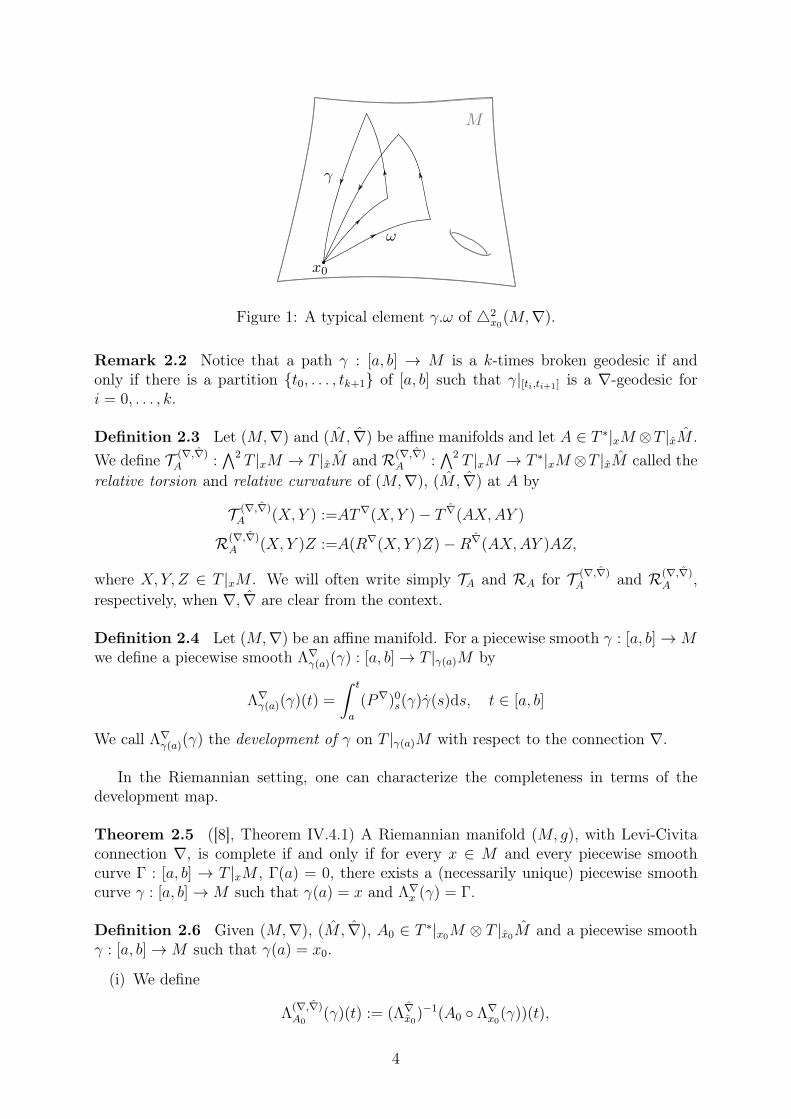
Figure 1: A typical element γ.ω of 2x0(M,∇).

Remark 2.2 Notice that a path γ : [a, b] → M is a k-times broken geodesic if andonly if there is a partition t0, . . . , tk+1 of [a, b] such that γ|[ti,ti+1] is a ∇-geodesic fori = 0, . . . , k.

Definition 2.3 Let (M,∇) and (M, ∇) be affine manifolds and let A ∈ T ∗|xM ⊗T |xM .

We define T (∇,∇)A :

∧2 T |xM → T |xM and R(∇,∇)A :

∧2 T |xM → T ∗|xM ⊗T |xM called therelative torsion and relative curvature of (M,∇), (M, ∇) at A by

T (∇,∇)A (X, Y ) :=AT∇(X, Y )− T ∇(AX,AY )

R(∇,∇)A (X, Y )Z :=A(R∇(X, Y )Z)−R∇(AX,AY )AZ,

where X, Y, Z ∈ T |xM . We will often write simply TA and RA for T (∇,∇)A and R(∇,∇)

A ,respectively, when ∇, ∇ are clear from the context.

Definition 2.4 Let (M,∇) be an affine manifold. For a piecewise smooth γ : [a, b] →Mwe define a piecewise smooth Λ∇

γ(a)(γ) : [a, b] → T |γ(a)M by

Λ∇γ(a)(γ)(t) =

∫ t

a

(P∇)0s(γ)γ(s)ds, t ∈ [a, b]

We call Λ∇γ(a)(γ) the development of γ on T |γ(a)M with respect to the connection ∇.

In the Riemannian setting, one can characterize the completeness in terms of thedevelopment map.

Theorem 2.5 ([8], Theorem IV.4.1) A Riemannian manifold (M, g), with Levi-Civitaconnection ∇, is complete if and only if for every x ∈ M and every piecewise smoothcurve Γ : [a, b] → T |xM , Γ(a) = 0, there exists a (necessarily unique) piecewise smoothcurve γ : [a, b] →M such that γ(a) = x and Λ∇

x (γ) = Γ.

Definition 2.6 Given (M,∇), (M, ∇), A0 ∈ T ∗|x0M ⊗ T |x0M and a piecewise smoothγ : [a, b] →M such that γ(a) = x0.

(i) We define

Λ(∇,∇)A0

(γ)(t) := (Λ∇x0)−1(A0 Λ

∇x0(γ))(t),

4

for all t ∈ [a, b] where defined. If c ∈ [a, b] is such that Λ(∇,∇)A0

(γ)(c) exists, we call

Λ(∇,∇)A0

(γ)|[a,c] the development of γ onto M through A0 with respect to (∇, ∇). We

will usually write simply ΛA0(γ) for Λ(∇,∇)A0

(γ) when there is no risk of confusion.

(ii) If Λ(∇,∇)A0

(γ)(t) is defined, we define the relative parallel transport of A0 along γ tobe the linear map

(P (∇,∇))ta(γ)A0 : T |γ(t)M → T |Λ(∇,∇)A0

(γ)(t)M ;

(P (∇,∇))ta(γ)A0 := (P ∇)ta(Λ

(∇,∇)A0

(γ)) A0 (P

∇)at (γ).

As before, one writes briefly P ta(γ)A0 for (P (∇,∇))ta(γ)A0 when the connections in

question are evident.

Remark 2.7 It is evident that Λ(∇,∇)A0

(γ)(t) exists for all t > a near a and if Λ(∇,∇)A0

(γ)(t)

exists for some t > a then Λ(∇,∇)A0

(γ)(t′) exists for all t′ ∈ [a, t] as well. By Theorem

2.5, if (M, g) is a complete Riemannian manifold with Levi-Civita connection ∇, the

development Λ(∇,∇)A0

(γ)(t) is defined for every t ∈ [a, b].

We record a lemma whose easy proof we omit.

Lemma 2.8 Let (M,∇) and (M, ∇) be affine manifold, A0 ∈ T ∗|x0M ⊗ T |x0M andγ : [a, b] →M a piecewise smooth path with γ(a) = x0.

(i) If ω : [c, d] →M is a piecewise smooth path such that γ(b) = ω(c), then

ΛA0(ω ⊔ γ) = ΛPba(γ)A0

(ω) ⊔ ΛA0(γ)

P ta(ω ⊔ γ)A0 =

P t

a(γ)A0, if t ∈ [a, b]

P t−b+cc (ω)Pb

a(γ)A0, if t ∈ [b, b+ d− c].

Moreover,

ΛA0(γ−1 ⊔ γ)(2b− a) = x0, P2b−a

a (γ−1 ⊔ γ)A0 = A0.

(ii) If γ : [a, b] → M is a k-times broken geodesic on (M,∇) and if ΛA0(γ)(t) exists forall t ∈ [a, b] then ΛA0(γ) is a k-times broken geodesic on (M, ∇). In particular, ifγu(t) := exp∇

x0(tu), γA0u(t) := exp∇

x0(tA0u), then ΛA0(γu) = γA0u.

(iii) Let γ : [a, b] → M be a piecewise smooth curve such that γ(a) = x0. Then γ =ΛA0(γ) if and only if

P at (γ)

˙γ(t) = A0Pat (γ)γ(t), t ∈ [a, b].

(iv) If X(·) is a vector field along γ : [a, b] → M , then for all t ∈ [a, b] such thatγ(t) := ΛA0(γ)(t) is defined, one has

∇ ˙γ(t)

((P t

a(γ)A0)X(t))= (P t

a(γ)A0)∇γ(t)X(t).

5

(v) Suppose φ : [α, β] → [a, b] is smooth and φ(t) 6= 0 ∀t ∈ [α, β]. Then the followinghold for all t ∈ [α, β] such that left or right hand side is defined:

ΛA0(γ)(φ(t)) = ΛA0(γ φ)(t)

Pφ(t)a (γ)A0 = P t

α(γ φ)A0.

Remark 2.9 Suppose γ, ω,Γ : [0, 1] → M are such that γ(1) = ω(0), ω(1) = Γ(0). Asremarked earlier, Γ.(ω.γ) 6= (Γ.ω).γ. Lemma 2.8, however, implies that

ΛA0((Γ.ω).γ)(1) =ΛA0(Γ.(ω.γ))(1)

P10 ((Γ.ω).γ)A0 =P1

0 (Γ.(ω.γ))A0

Indeed, the latter (which implies the former) follows by computing

P10 ((Γ.ω).γ)A0 =P1

0 (Γ.ω)P10 (γ)A0 = P1

0 (Γ)P10 (ω)P

10 (γ)A0 = P1

0 (Γ)P10 (ω.γ)A0

=P10 (Γ.(ω.γ))A0.

We recall next the Cartan-Ambrose-Hicks theorem (C-A-H Theorem for short) in thecontext of Riemannian manifolds of equal dimension.

Theorem 2.10 (C-A-H) ([2, 3, 10, 12]) Let (M, g) and (M, g) be complete Riemannianmanifolds of the same dimension, dimM = dim M , and let A0 ∈ T ∗|x0M ⊗ T |x0M be aninfinitesimal isometry. Then there exists a complete Riemannian manifold (N, h), z0 ∈ Nand Riemannian covering maps F : (N, h) → (M, g), G : (N, h) → (M, g) such thatG∗|z0 = A0 F∗|z0 if and only if

R(∇,∇)

P10 (γ)A0

= 0, ∀γ ∈ ∠x0(M,∇), (1)

where ∇, ∇ are the Levi-Civita connections of (M, g) and (M, g).

3 Main Result

We begin this section with the statement of the main theorem of the paper. The resultwill then be followed by two corollaries and some remarks. The proof of the theorem ispostponed to section 4.

Theorem 3.1 Suppose (M, g), (M, g) are complete Riemannian manifolds of the samedimension, dimM = dim M , M simply connected and let A0 ∈ T |x0M ⊗ T |x0M be aninfinitesimal isometry. Then there exists a Riemannian covering map f : M → M withf∗|x0 = A0 if and only if

Λ(∇,∇)A0

(2

x0(M,∇)

)⊂ Ωx0(M), (2)

where ∇, ∇ are the Levi-Civita connections of (M, g), (M, g), respectively.

Remark 3.2 Notice that by Lemma 2.8 (ii) the condition (2) is equivalent to

Λ(∇,∇)A0

(2

x0(M,∇)

)⊂ 2

x0(M, ∇)

and that it is implied by the condition

Λ(∇,∇)A0

(Ωx0(M)

)⊂ Ωx0(M). (3)

6

If one wishes not to assume M to be simply connected in Theorem 3.1, then the resultcan be modified as follows:

Corollary 3.3 Suppose (M, g), (M, g) are complete Riemannian manifolds of the samedimension, dimM = dim M and let A0 ∈ T |x0M ⊗ T |x0M be and infinitesimal isometry.The condition (2) holds if and only if there exists a complete simply connected Riemannianmanifold (N, h), Riemannian covering maps F : N →M , G : N → M and a z0 ∈ N suchthat G∗|z0 = A0 F∗|z0 and

Γ(1) | Γ : [0, 1] → N continuous, Γ(0) = z0, F Γ ∈ 2x0(M,∇) ⊂ G−1(x0), (4)

Proof. Sufficiency. Let (N, h) and the maps F,G be given as stated and suppose (4)is true. For a γ ∈ 2

x0(M,∇), let Γ be the unique path in N such that γ = F Γ

and Γ(0) = z0. It follows that G Γ = ΛA0(γ) and since Γ(1) ∈ G−1(x0), we haveΛA0(γ)(1) = G(Γ(1)) = x0 i.e. (2) holds.

Necessity. Let F : N →M be the universal covering of M and lift the metric g onto N ,which we denote by h. As is well known, (N, h) is complete. Fix a point z0 ∈ F−1(x0) andwrite D for the Levi-Civita connection of (N, h). Let B0 := A0 F∗|z0 ∈ T ∗|z0N ⊗ T |x0Mwhich is an infinitesimal isometry and notice that if Γ : [0, 1] → N is a piecewise smoothpath starting from z0, then ΛB0(Γ) = ΛA0(F Γ). In particular, if Γ ∈ 2

z0(N,D), then

F Γ ∈ 2x0(M,∇) and hence ΛB0(Γ) ∈ Ωx0(M) by assumption (2).

Thus Theorem 3.1 implies the existence of a Riemannian covering map G : N → Msuch that G∗|z0 = B0 = A0 F∗|z0 . To prove (4), let Γ : [0, 1] → N be such that Γ(0) = z0and F Γ ∈ 2

x0(M,∇). Then G Γ = ΛB0(Γ) = ΛA0(F Γ) ∈ Ωx0(M) so in particular,

G(Γ(1)) = ΛA0(F Γ)(1) = x0 i.e. Γ(1) ∈ G−1(x0). The proof is complete.

Remark 3.4 If the the previous corollary one replaces the condition (2) by (3), then(4) can be replaced by the condition F−1(x0) ⊂ G−1(x0). This is clear from the proof ofthe corollary.

The above theorem has an easy corollary.

Corollary 3.5 Let (M, g), (M, g) be complete Riemannian manifolds of the same di-mension, dimM = dim M . Given an infinitesimal isometry A0 ∈ T |x0M ⊗ T |x0M andx1 ∈ M , x1 ∈ M , then there exists a Riemannian covering map f : M → M withf∗|x0 = A0 and f(x1) = x1 if and only if

∀ 6-broken geodesic γ : [0, 1] →M s.t. γ(0) = x0, γ(1) = x1 =⇒ Λ(∇,∇)A0

(γ)(1) = x1.

Proof. Necessity. Suppose we are given a Riemannian covering map f : M → M withf∗|x0 = A0 and f(x1) = x1. Then if γ is a 6-broken geodesic with γ(0) = x0, γ(1) = x1, itfollows that ΛA0(γ) = f γ and hence ΛA0(γ)(1) = f(γ(1)) = f(x1) = x1.

Sufficiency. Let Γ : [0, 1] → M be any geodesic from x0 to x1 (such a geodesic existssince (M, g) is complete) and define A1 := P1

0 (Γ)A0. Taking any γ, ω ∈ x1(M,∇), wesee that (see Lemma 2.8)

ΛA1(γ.ω)(1) = ΛP10 (Γ)A0

(γ.ω)(1) = ΛA0((γ.ω).Γ)(1) = x1,

where the last equality follows from the fact that (γ.ω).Γ is a 6-broken geodesic that startsfrom x0 and ends to x1. Thus ΛA1(

2x1(M,∇)) ⊂ Ωx1(M) and Theorem 3.1 implies that

7

there is a covering map f : M → M such that f∗|x1 = A1. In particular, f(x1) = x1.Moreover,

f∗|Γ−1(t) = P t0(Γ

−1)A1 = P1−t0 A0,

which implies that f∗|x0 = f∗|Γ−1(1) = P00A0 = A0. The proof is finished.

Remark 3.6 The condition of the corollary means that 6-times broken geodesics of M

with end points x0 and x1 map by the development Λ(∇,∇)A0

to 6-times broken geodesics of

M with end points x0 and x1.Also observe that this condition is implied by the following stronger one:

∀ γ : [0, 1] →M, piecewise smooth s.t. γ(0) = x0, γ(1) = x1 =⇒ Λ(∇,∇)A0

(γ)(1) = x1.

4 Proof of the Main Result

The proof of Theorem 3.1 (see p.15) makes use of the following key proposition which westate and prove in a more general setting of affine manifolds.

Proposition 4.1 Suppose that (M,∇), (M, ∇) are affine manifolds (possibly of differentdimensions) and let A0 ∈ T |x0M ⊗ T |x0M be given. Let U ⊂ T |x0M , U ⊂ T |x0M bethe domains of definitions of exp∇

x0, exp∇

x0, respectively, and write γu(t) = exp∇

x0(tu),

γu(t) = exp∇x0(tu) for u ∈ U , u ∈ U . Then if

Λ(∇,∇)A0

(x0 (M,∇)

)⊂ x0(M, ∇) (5)

T (∇,∇)

P10 (γu)A0

(γu(1), ·) = 0, ∀u ∈ U ∩ A−10 (U), (6)

hold, one has for all u ∈ U ∩ A−10 (U) that

(P ∇)01(γA0u) (exp∇x0)∗|A0u A0 = A0 (P

∇)01(γu) (exp∇x0)∗|u (7)

R(∇,∇)

P10 (γu)A0

(γu(1), ·)γu(1) = 0. (8)

Remark 4.2 Since Λ(∇,∇)A0

(γ) might not be defined on whole interval [0, 1] for every γ ∈

x0(M,∇), except if e.g. (M, ∇) is geodesically complete, we understand the assumption

(5) to mean that if γ ∈ x0(M,∇) and if Λ(∇,∇)A0

(γ) is defined on [0, 1], then Λ(∇,∇)A0

(γ) ∈

x0(M, ∇).

Proof. We will not make the assumption Eq. (6) until later on. Notice also that U and Uare star-shaped around the origin of T |x0M and hence so is U ∩A−1

0 (U). In the proof wewrite γX(t) = exp∇

x (tX) and γX(t) = exp∇x (tX) whenever x ∈M , x ∈ M and X ∈ T |xM ,

X ∈ T |xM and t ∈ R are such that these are defined. If they are defined for all t ∈ [0, 1],we assume, by default, that the domains of definitions of γX and γX are the interval [0, 1].

Given u ∈ U ∩ A−10 (U) and v ∈ T |x0M we define a vector field along γu by

Yu,v(t) :=∂

∂s

∣∣0exp∇

x0(t(u+ sv)) = t(exp∇

x0)∗|tu(v)

8

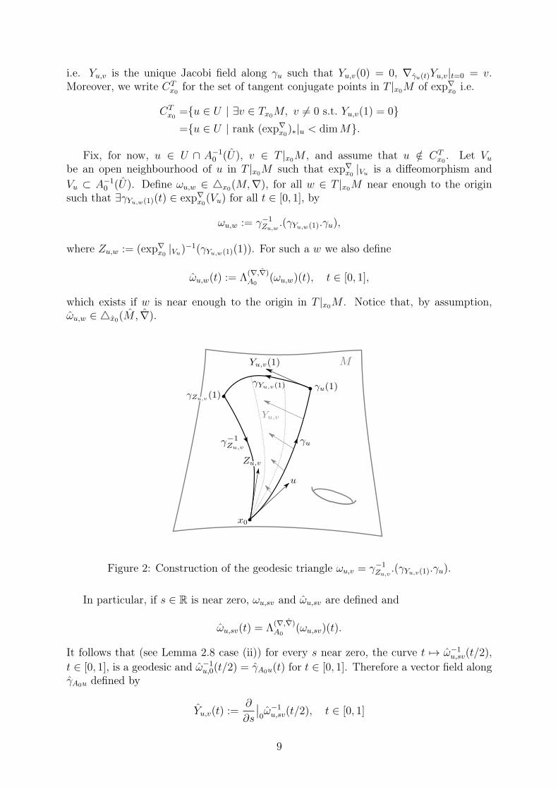
i.e. Yu,v is the unique Jacobi field along γu such that Yu,v(0) = 0, ∇γu(t)Yu,v|t=0 = v.Moreover, we write CT

x0for the set of tangent conjugate points in T |x0M of exp∇

x0i.e.

CTx0

=u ∈ U | ∃v ∈ Tx0M, v 6= 0 s.t. Yu,v(1) = 0

=u ∈ U | rank (exp∇x0)∗|u < dimM.

Fix, for now, u ∈ U ∩ A−10 (U), v ∈ T |x0M , and assume that u /∈ CT

x0. Let Vu

be an open neighbourhood of u in T |x0M such that exp∇x0|Vu

is a diffeomorphism andVu ⊂ A−1

0 (U). Define ωu,w ∈ x0(M,∇), for all w ∈ T |x0M near enough to the originsuch that ∃γYu,w(1)(t) ∈ exp∇

x0(Vu) for all t ∈ [0, 1], by

ωu,w := γ−1Zu,w

.(γYu,w(1).γu),

where Zu,w := (exp∇x0|Vu

)−1(γYu,w(1)(1)). For such a w we also define

ωu,w(t) := Λ(∇,∇)A0

(ωu,w)(t), t ∈ [0, 1],

which exists if w is near enough to the origin in T |x0M . Notice that, by assumption,ωu,w ∈ x0(M, ∇).

Figure 2: Construction of the geodesic triangle ωu,v = γ−1Zu,v

.(γYu,v(1).γu).

In particular, if s ∈ R is near zero, ωu,sv and ωu,sv are defined and

ωu,sv(t) = Λ(∇,∇)A0

(ωu,sv)(t).

It follows that (see Lemma 2.8 case (ii)) for every s near zero, the curve t 7→ ω−1u,sv(t/2),

t ∈ [0, 1], is a geodesic and ω−1u,0(t/2) = γA0u(t) for t ∈ [0, 1]. Therefore a vector field along

γA0u defined by

Yu,v(t) :=∂

∂s

∣∣0ω−1u,sv(t/2), t ∈ [0, 1]

9

is a Jacobi field. Since ω−1u,sv(0) = ωu,sv(1) = x0, we have that Yu,v(0) = 0 which implies

that there is a unique v(u, v) ∈ T |x0M such that

Yu,v(t) =∂

∂s

∣∣0exp∇

x0(t(A0u+ sv(u, v))) = t(exp∇

x0)∗|tA0u(v(u, v)), t ∈ [0, 1], (9)

i.e. v(u, v) = ∇ ˙γA0u(t)Yu,v(t)|t=0. Notice that Yu,v(t), and hence also v(u, v), is well defined

for all (u, v) ∈ (U ∩A−10 (U)\CT

x0)×T |x0M and t ∈ [0, 1] and it is clear that v is a smooth

map.We will now state and prove three lemmas and come back to the proof of the propo-

sition after them.

Lemma 4.3 Under the above assumptions, one has

∇ ˙γu(t)Yu,v|t=1 = (P1

0 (γu)A0)∇γu(t)Yu,v|t=1 − TP10 (γu)A0

(γu(1), Yu,v(1)). (10)

for all (u, v) ∈ (U ∩ A−10 (U) \ CT

x0)× T |x0M .

Proof. In the proof we always assume that s ∈ R that appears is near zero. Then we mayassume that ωu,sv, ωu,sv and Yu,sv are defined.

Writing ∂t := ∂∂texp∇

x0(t(u + sv)), ∂s := ∂

∂sexp∇

x0(t(u + sv)) ∂t :=

∂∂tω−1u,sv(t/2), ∂s :=

∂∂sω−1u,sv(t/2), we have (here ∂

∂t|1− means the left hand side derivative at t = 1)

∇ ˙γA0u(t)Yu,v|t=1 − T ∇(∂t, ∂s)|(t,s)=(1,0)

=∇∂t

∂

∂s

∣∣∣0ω−1u,sv(t/2)

∣∣∣t=1−

− T ∇(∂t, ∂s)|(t,s)=(1,0)

=∇∂s

∂

∂t

∣∣∣1−ω−1u,sv(t/2)

∣∣∣s=0

= −∇∂s

∂

∂t

∣∣∣1−ωu,sv(1− t/2)

∣∣∣s=0

=− ∇∂s

(P1/2

0 (ωu,sv)A0∂

∂t

∣∣∣1−ωu,sv(1− t/2)

)∣∣∣s=0

=∇∂s

(P1

0 (γYu,sv(1).γu)A0∂

∂t

∣∣1exp∇

x0(tZu,sv)

)∣∣∣s=0

where at the second to last equality we used the fact that ˙ωu,sv(t) = (P t0(ωu,sv)A0)ωu,sv(t),

t ∈ [0, 1] (using one-sided derivatives at break points); see Lemma 2.8 case (iii). Noticethat Yu,sv(t) = sYu,v(t) and so γYu,sv(1)(t) = γsYu,v(1)(t) = γYu,v(1)(ts), which leads us toconclude that if s > 0,

P10 (γYu,sv(1).γu)A0 =P1

0 (t 7→ γYu,v(ts))P1

0 (γu)A0 = Ps0(γYu,v(1))P

10 (γu)A0.

Therefore

∇ ˙γA0u(t)Yu,v|t=1 − T ∇(∂t, ∂s)|(t,s)=(1,0)

=∇∂s

((Ps

0(γYu,v(1))P10 (γu)A0)

∂

∂t

∣∣1exp∇

x0(tZu,sv)

)∣∣∣s=0+

=(P1

0 (γu)A0

)∇∂s

( ∂∂t

∣∣1exp∇

x0(tZu,sv)

)∣∣s=0

=(P1

0 (γu)A0

)(∇γu(t)

( ∂∂s

∣∣0exp∇

x0(tZu,sv)

)∣∣t=1

+ T (∂s, ∂t)|(t,s)=(1,0)

),

10

where at the second to last equality we used Lemma 2.8 case (iv) (notice that s 7→∂∂t

∣∣1exp∇

x0(tZu,sv) is a vector field along s 7→ γYu,v(1)(s) = γYu,sv(1)(1)) and at the last

equality we noticed that Zu,0 = u, so ∂∂texp∇

x0(tZu,sv)

∣∣s=0

= γu(t) = ∂t. At this momentwe make the following observations:

∂t|(t,s)=(1,0) =(P10 (γu)A0)∂t|(t,s)=(1,0)

∂s|(t,s)=(1,0) =Yu,v(1),

∂s|(t,s)=(1,0) =Yu,v(1) =∂

∂s

∣∣0ω−1u,sv(1/2) =

∂

∂s

∣∣0ωu,sv(1/2) =

∂

∂s

∣∣0ΛA0(γYu,sv(1).γu)(1)

=∂

∂s

∣∣0ΛP1

0 (γu)A0(γYu,sv(1))(1) =

∂

∂s

∣∣0γ(P1

0 (γu)A0)Yu,sv(1)(1)

=∂

∂s

∣∣0γ(P1

0 (γu)A0)Yu,v(1)(s) = (P10 (γu)A0)Yu,v(1).

These allow us to write the above equation into the form

∇ ˙γA0u(t)Yu,v|t=1 + TP1

0 (γu)A0(γu(1), Yu,v(1)) =

(P1

0 (γu)A0

)∇γu(t)

( ∂∂s

∣∣0exp∇

x0(tZu,sv)

)∣∣t=1.

Therefore, it remains to show that ∂∂s

∣∣0exp∇

x0(tZu,sv) = Yu,v(t), ∀t ∈ [0, 1]. Indeed,

J(t) := ∂∂s

∣∣0exp∇

x0(tZu,sv) is a Jacobi field along γu and it satisfies the boundary conditions

J(0) = 0 = Yu,v(0) and

J(1) =∂

∂s

∣∣0exp∇

x0(Zu,sv) =

∂

∂s

∣∣0γYu,sv(1)(1) =

∂

∂s

∣∣0γYu,v(1)(s) = Yu,v(1).

Since u /∈ CTx0

, it follows that J = Yu,v and thus the proof is finished.

From the last proof, we record for later use the following fact:

Yu,v(1) = (P10 (γu)A0)Yu,v(1), (11)

for all (u, v) ∈ (U ∩ A−10 (U)\CT

x0)× T |x0M .

Lemma 4.4 Under the above assumptions, for all (u, v) ∈ (U ∩A−10 (U) \CT

x0)× T |x0M

the following holds:

(exp∇x0)∗|A0u(∂1v(u, v)(u)) = TP1

0 (γu)A0(γu(1), Yu,v(1)).

Hence in particular,

TA0 = 0.

Proof. By assumption, u ∈ U ∩ A−10 (U) \ CT

x0and so for all t near 1, one has tu ∈

U ∩A−10 (U) \CT

x0. In the proof of the first claim, we assume always that t is near enough

to 1 so that this is the case.Since Ytu,v(1) = 1

tYu,v(t), Eq. (11) implies that

tYtu,v(1) = t(P10 (γtu)A0)Ytu,v(1) = (P t

0(γu)A0)Yu,v(t).

11

Writing ∂t := γu(t), ∂t := ˙γA0u(t) to simplify the notation, we have

Yu,v(1) + ∇∂tYtu,v(1)|t=1 = ∇∂t

(tYtu,v(1))|t=1 = ∇∂t

((P t

0(γu)A0)Yu,v(t))|t=1

=(P t0(γu)A0)∇∂tYu,v(t)|t=1 = ∇∂tYu,v(t)|t=1 + TP1

0 (γu)A0(γu(1), Yu,v(1)),

where at the third equality we used Lemma 2.8 case (iv) and at the fourth equality weused (10). But

∇∂tYu,v(t)|t=1 = ∇∂t

(t(exp∇

x0)∗|tA0u(v(u, v))

)∣∣t=1

=(expx0)∗|A0u(v(u, v)) + ∇∂t

((exp∇

x0)∗|tA0u(v(u, v))

)∣∣t=1

=Yu,v(1) + ∇∂t

((exp∇

x0)∗|tA0u(v(u, v))

)∣∣t=1,

while

∇∂tYtu,v(1)|t=1 = ∇∂t

((exp∇

x0)∗|tA0u(v(tu, v))

)∣∣t=1,

so combining these three formulas, one gets

TP10 (γu)A0

(γu(1), Yu,v(1)) =∇∂t

((exp∇

x0)∗|tA0u(v(tu, v))

)∣∣t=1

− ∇∂t

((exp∇

x0)∗|tA0u(v(u, v))

)∣∣t=1

=∇∂t

((exp∇

x0)∗|tA0u

(v(tu, v)− v(u, v)

))∣∣t=1.

Writing ∂1v(u, v)(X) for the differential of v at (u, v) with respect to v in the directionX, we have

v(tu, v)− v(u, v) =

∫ t

1

∂

∂sv(su, v)ds =

∫ t

1

∂1v(su, v)(u)ds.

Notice that (exp∇x0)∗|tA0u ∈ T ∗(T |x0M)⊗TM for t ∈ [0, 1], so if we write D for the vector

bundle connection on T ∗(T |x0M)⊗TM → T |x0M×M naturally induced by the canonicalconnection on vector space T |x0M and ∇, we get finally

TP10 (γu)A0

(γu(1), Yu,v(1)) = ∇∂t

((exp∇

x0)∗|tA0u

(∫ t

1

∂1v(su, v)(u)ds))∣∣∣

t=1

=(D d

dt(tA0u,γA0u

(t))(exp∇x0)∗|tA0u

)∣∣∣t=1

∫ 1

1

∂1v(su, v)(u)ds

+ (exp∇x0)∗|A0u

d

dt

∣∣t=1

∫ t

1

∂1v(su, v)(u)ds

=(exp∇x0)∗|A0u(∂1v(u, v)(u)),

which proves the first part of the lemma.It remains to prove that TA0 = 0. Indeed, by what was just proved, we have that for

all u, v ∈ T |x0M and for all t small,

(exp∇x0)∗|tu(∂1v(tu, v)(tu)) = TP(γtu,A0)(1)(γtu(1), Ytu,v(1))

holds i.e., because Ytu,v(1) = 1tYu,v(t),

t(exp∇x0)∗|tu(∂1v(tu, v)(u)) = TP(γu,A0)(t)(γu(t),

1

tYu,v(t)).

But as t → 0, one has 1tYu,v(t) → ∇γu(t)Yu,v|t=0 = v, ∂1v(tu, v)(u) → ∂1v(0, v)(u) and

P(γu, A0)(t) → A0, so in the limit one gets 0 = TA0(u, v). Since u, v ∈ T |x0M werearbitrary, the result follows.

12

From now on we will make all the assumption in the statement of Proposition 4.1 i.e.we also include the torsion condition Eq. (6).

Lemma 4.5 Under the above assumptions and for all (u, v) ∈ (U∩A−10 (U)\CT

x0)×T |x0M

and t ∈ [0, 1], one has

Yu,v(t) =∂

∂s

∣∣0exp∇

x0(tA0(u+ sv)) (12)

Yu,v(t) =(P t0(γu)A0)Yu,v(t). (13)

Proof. Write CTx0

for the tangent conjugate set of (M, ∇) at x0 defined in the same way

as CTx0

. By Lemma 4.4 and condition (6), one has (exp∇x0)∗|A0u(∂1v(u, v)(u)) = 0 for all

(u, v) ∈ (U∩A−10 (U)\CT

x0)×T |x0M . Given such a (u, v), if A0u /∈ CT

x0, then ∂1v(u, v)(u) =

0. Otherwise A0u ∈ CTx0

, but then ∃ǫ > 0 such that tu ∈ U ∩A−10 (U)\CT

x0and tA0u /∈ CT

x0

for all t ∈]1 − ǫ, 1 + ǫ[\1, hence ∂1v(tu, v)(tu) = 0. Letting t → 1 then implies that∂1v(u, v)(u) = 0. Therefore we have shown that

∂1v(u, v)(u) = 0, ∀(u, v) ∈ (U ∩ A−10 (U)\CT

x0)× T |x0M.

Now fix u ∈ U∩A−10 (U)\CT

x0and v ∈ T |x0M . Notice that the set S := t ∈ [0, 1] | tu ∈

CTx0 is finite or empty. If S 6= ∅, we write S = tii=1,...,N where 0 < ti < ti+1 < 1 for all

i and we set tN+1 := 1. In the case where S is empty, we set t1 := 1, N := 0.Write t0 := 0 and notice that for t, τ ∈]ti, ti+1[ we have

v(tu, v) = v(τu, v) +

∫ t

τ

1

s∂1v(su, v)(su)︸︷︷︸

=0

ds = v(τu, v),

i.e. the value of t 7→ v(tu, v) is constant on each interval ]ti, ti+1[, i = 0, . . . , N . Letvi(u, v) be the constant value of v(tu, v) for t ∈]ti, ti+1[.

Define Ju,v(t), t ∈ [0, 1]\S, by

Ju,v(t) := t(exp∇x0)∗|tA0u(v(tu, v)), if t ∈]ti, ti+1[.

Then Ju,v is a Jacobi field on each interval ]ti, ti+1[ since for t ∈]ti, ti+1[.

Ju,v(t) = t(exp∇x0)∗|tA0u(vi(u, v)) =

∂

∂s

∣∣0exp∇

x0

(t(A0u+ svi(u, v))

).

But we observe that

Ju,v(t) = tYtu,v(1) = (P t0(γu)A0)Yu,v(t), ∀t ∈ [0, 1]\S,

hence because t 7→ (P t0(γu)A0)Yu,v(t) is smooth and S is finite, we see that Ju,v(t) uniquely

extends to a Jacobi field along γA0u defined on the whole interval [0, 1]. We still denotethis Jacobi field by Ju,v(t) and notice that since

Ju,v(t) = t(exp∇x0)∗|tA0u(v0(u, v))

holds for t ∈]0, t1[, it holds for all t ∈ [0, 1].

13

To identify Ju,v(t) once and for all, it remains to compute the value of v0(u, v). Wehave

v(0, v) =(exp∇x0)∗|0(v(0, v)) = Y0,v(1) = (P1

0 (γ0)A0)Y0,v(1)

=A0Y0,v(1) = A0(exp∇x0)∗|0(v) = A0v

and thus v0(u, v) = limt→0+ v(tu, v) = v(0, v) = A0v. We have thus shown the following:

(exp∇x0)∗|A0u(v(u, v)) = Yu,v(1) = Ju,v(1) = (exp∇

x0)∗|A0u(A0v).

We will prove that v(u, v) = A0v. Indeed, if A0u /∈ CTx0

, then the above equationreadily implies that v(u, v) = A0v. On the other hand, if A0u ∈ CT

x0, then for all t 6= 1

near 1, one has tA0u /∈ CTx0

and (exp∇x0)∗|tA0u(v(tu, v) − A0v) = 0, which implies that

v(tu, v) = A0v and finally v(u, v) = A0v by passing to the limit t→ 1.Since v(u, v) = A0v, the claimed eq. (12) follows from (9). To prove (13), notice that

(P t0(γu)A0)Yu,v(t) = tYtu,v(1) = t

∂

∂s

∣∣0exp∇

x0(A0(tu+ sv)) = t(exp∇

x0)∗|tA0u(A0v) = Yu,v(t).

This concludes the proof.

We are now ready to finish the proof of the proposition. Let u ∈ U ∩ A−10 (U)\CT

x0.

Because Yu,v(1) = (exp∇x0)∗|u(v) by definition and since Yu,v(1) = (exp∇

x0)∗|A0u(A0v), by

(12), the formula (7) is an immediate consequence of (13) and Definition 2.6. Since CTx0

has no interior points in T |x0M , it follows that (7) holds for all u ∈ U ∩ A−10 (U).

It remains to prove the formula (8). Let (u, v) ∈ U ∩ A−10 (U)\CT

x0× T |x0M . Taking

twice the covariant derivative w.r.t. ∇ ˙γA0u(t) of both sides of the equation (13), recalling

that Yu,v, Yu,v are Jacobi fields and using Lemma 2.8 case (iv), we get

R∇( ˙γA0u(t), Yu,v(t))˙γA0u(t) + ∇ ˙γA0u

(t)

(T ∇( ˙γA0u(t), Yu,v(t))

)

=∇ ˙γA0u(t)∇ ˙γA0u

(·)Yu,v(·) = (P t0(γu)A0)∇γu(t)∇γu(·)Yu,v(·)

=(P t0(γu)A0)

(R∇(γu(t), Yu,v(t))γu(t) +∇γu(t)

(T∇(γu(t), Yu,v(t))

)).

Using the last two equations above, the fact that ˙γA0u(t) = P(γu, A0)(t)γu(t) and Defini-tion 2.3 we get that, for all (u, v) ∈ U ∩ A−1

0 (U)\CTx0

× T |x0M ,

RPt0(γu)A0

(γu(t), Yu,v(t))γu(t) = −∇ ˙γA0u(t)TP·

0(γu)A0(γu(·), Yu,v(·)) = 0,

since TPt0(γu)A0

(γu(t), Yu,v(t)) = TP10 (γtu)A0

(γtu(1), Ytu,v(1)) = 0, t ∈ [0, 1], by assumtion (6).Let then u ∈ U ∩ A−1

0 (U) and let 0 < t1 < t2 < . . . be the conjugate times along γu(i.e t1u, t2u, . . . = tu | t ∈ [0, 1] ∩ CT

x0). Suppose X(t) is any vector field along γu. If

t 6= tj for all j, then there is a v(t) ∈ T |x0M such that Yu,v(t)(t) = X(t), and so

RPt0(γu)A0

(γu(t), X(t))γu(t) = 0.

By continuity, this holds for all t ∈ [0, 1] and hence the result follows once we set t = 1.

14

Remark 4.6 Notice that (5) is equivalent to the condition

Λ(∇,∇)A0

(x0 (M,∇)

)⊂ Ωx0(M).

On the other hand, if (5) is replaced by a stronger condition

Λ(∇,∇)A0

(Ωx0(M)) ⊂ Ωx0(M),

then in the proof one can define ωu,v to be γ−1u+v.

((s 7→ γu+sv(1)).γu

)∈ Ωx0(M). Then ωu,v

and hence ωu,v, Yu,v and finally v(u, v) are defined for all (u, v) ∈ (U ∩A−10 (U))× T |x0M .

The proof goes through in the same way as above, all the lemmas 4.3-4.5 being true evenwith the set U ∩A−1

0 (U)\CTx0

replaced with U ∩A−10 (U) everywhere. Moreover, the proof

becomes slightly easier since one does not need to pay attention to the tangent conjugateset CT

x0.

We will now proceed to the proof of Theorem 3.1.

Proof. (of Theorem 3.1) Necessity. If f :M → M is a Riemannian covering with f∗|x0 =A0, then for γ ∈ 2

x0(M,∇), one has ΛA0(γ) = f γ and hence ΛA0(γ)(1) = f(γ(1)) =

f(x0) = x0. So ΛA0(γ) ∈ Ωx0(M).Sufficiency. The idea is to prove, using Proposition 4.1, that the condition of C-A-H

Theorem 2.10 given by Eq. (1) holds, which then implies the claim.Define

A := P10 (γ)A0 | γ ∈ x0(M,∇)

and notice that assumption (5) implies that A ⊂ T ∗|x0M ⊗ T |x0M and it is clear thateach A ∈ A is an infinitesimal isometry.

We claim that

P 01 (γAu) (exp

∇x0)∗|Au A = A P 0

1 (γu) (exp∇x0)∗|u, ∀A ∈ A, u ∈ T |x0M. (14)

Indeed, fix A ∈ A and let ω ∈ x0(M,∇) be arbitrary. Then there is an γ ∈ x0(M,∇)such that A = P1

0 (γ)A0. But then ω.γ ∈ 2x0(M,∇) and hence by Lemma 2.8 (i) and the

assumptions of the theorem,

ΛA(ω)(1) =(ΛP1

0 (γ)A0(ω).ΛA0(γ)

)(1) = ΛA0(ω.γ)(1) = x0

i.e. ΛA(x0(M,∇)) ⊂ x0(M, ∇). Thus the above claim follows from Proposition 4.1.For a unit vector u ∈ T |x0M , let τ(u) ∈]0,+∞] be cut-time for the geodesic γu and

set

UT := tu | u ∈ T |x0M, ‖u‖g = 1, 0 ≤ t < τ(u), U := expx0(UT ).

For every A ∈ A one defines a map

φA : U → M ; φA = exp∇x0A (exp∇

x0|UT )−1.

We are to show that each φA is an isometry onto its open image. Indeed, if x ∈ U andX ∈ T |xM , let u = (expx0

|UT )−1(x) and use (14) to compute

‖(φA)∗(X)‖g =∥∥(P 1

0 (γAu) A P 01 (γu))X

∥∥g=∥∥(A P 0

1 (γu))X∥∥g=∥∥P 0

1 (γu)X∥∥g= ‖X‖g .

15

Since dimM = dim M , it follows that φA is a diffeomorphism onto its (open) image andis isometric. This settles the claim.

Knowing this, we may now show a property which then allows us (eventually) to callfor the C-A-H Theorem 2.10: For all A ∈ A and all unit vectors u ∈ T |x0M ,

RPt0(γu)A

= 0, ∀t; 0 ≤ t ≤ τ(u) (15)

with the understanding that 0 ≤ t ≤ τ(u) is replaced by t ≥ 0 if τ(u) = +∞. To provethis, notice that since φA is an isometry onto its open image, one has

(φA)∗(R∇((X, Y )Z

)= R∇(((φA)∗X, (φA)∗Y )((φA)∗Z), ∀x ∈ U, X, Y, Z ∈ T |xM

i.e. R(φA)∗|x = 0 for all x ∈ U . But we know from (14) that if 0 ≤ t < τ(u) (whencetu ∈ UT ), one has (φA)∗|γu(t) = P t

0(γAu) A P 0t (γu), which equals to P t

0(γu)A. HenceRPt

0(γu)A= 0 if 0 ≤ t < τ(u) and by continuity this also holds when t = τ(u) (if

τ(u) < +∞) which establishes the claim.We are now ready to finish the proof by appealing to C-A-H Theorem 2.10. Indeed,

let ω ∈ ∠x0(M,∇). Since (M, g) is complete, there exists a unit vector u ∈ T |x0M suchthat γu : [0, τ(u)] → M is a minimal geodesic from x0 to ω(1). Because then γ−1

τ(u)u.ω ∈

x0(M,∇), one has that A := P10 (γ

−1τ(u)u.ω)A0 is in A and therefore R

Pτ(u)0 (γu)A

= 0 by

(15). But by Lemma 2.8,

Pτ(u)0 (γu)A =P1

0 (γτ(u)u)P10 (γ

−1τ(u)u.ω)A0 = P1

0 (γτ(u)u)P10 (γ

−1τ(u)u)P

10 (ω)A0 = P1

0 (ω)A0,

which proves that RP10 (ω)A0

= 0 for all ω ∈ ∠x0(M,∇).Therefore the condition (1) of C-A-H Theorem 2.10 is satisfied and hence there exists

a complete Riemannian manifold (N, h), z0 ∈ N and Riemannian covering maps F :N → M , G : N → M such that A0 = G∗|z0 (F∗|z0)

−1. Since M is simply connected,F : N →M is a Riemannian isomorphism and setting f := G F−1 finishes the proof.

Remark 4.7 In the case where there are no cut-points on any geodesic of (M, g) ema-nating from x0, then one may replace (2) in Theorem 3.1 by the condition

Λ(∇,∇)A0

(x0(M,∇)) ⊂ Ωx0(M).

Indeed, in this case exp∇x0

: T |x0M → M is a diffeomorphism and in the above proofUT = T |x0M , U =M and so φA0 :M → M is an isometry onto its open image. It followsfrom a standard result on Riemannian manifolds that f := φA0 is a covering map andobviously f∗|x0 = A0.

5 Different Formulations of the Cartan-Ambrose-Hicks

Theorem

In this section, we will complement the C-A-H theorem 2.10 by giving eight equivalentcharacterizations for the existence of a Riemannian covering map f : (M, g) → (M, g)(under specific assumptions).

First we recall a well-known proposition and, for the sake of completeness, give itseasy proof.

16

Proposition 5.1 Suppose (M,∇), (M, ∇) are affine manifolds such that M is simplyconnected and geodesically accessible from x0 and that (M, ∇) is geodesically complete.Given A0 ∈ T |x0M ⊗ T |x0M , there exists an affine map f :M → M such that f∗|x0 = A0

if and only if

(P (∇,∇))10(γ)A0 = A0, ∀γ ∈ x0(M,∇). (16)

Proof. Necessity. If f : M → M is an affine map such that f∗|x0 = A0 and if γ ∈

x0(M,∇), then ΛA0(γ) = f γ and hence ΛA0(γ)(1) = f(γ(1)) = f(x0) = x0.

Sufficiency. In the proof we write γu(t) = exp∇x (tu), when u ∈ T |xM . Let x ∈ M be

given. Let γ, ω ∈ ∠x0(M,∇) be such that γ(1) = x, ω(1) = x, which exist since (M,∇)is geodesically accessible from x0. Then ω−1.γ ∈ x0

(M,∇) and hence

P10 (ω

−1.γ)A0 = A0.

It follows that (see Lemma 2.8 and Remark 2.9)

ΛA0(ω)(1) =ΛP10 (ω

−1.γ)A0(ω)(1) = ΛA0(ω.(ω

−1.γ))(1) = ΛA0((ω.ω−1).γ)(1)

=ΛP10 (γ)A0

(ω.ω−1)(1) = ΛA0(γ)(1).

This shows that if for x ∈M one defines

f(x) := ΛA0(γ)(1) | γ ∈ ∠x0(M,∇), γ(1) = x,

then f(x) is a singleton set for all x ∈M and hence f can be seen as a map f :M → M .We show that f is an affine map. To do that, we first make a construction for its

differential that is analogous to that for f above. Let x ∈ M and let γ, ω ∈ ∠x0(M,∇)be such that γ(1) = x, ω(1) = x as above, then since ω−1.γ ∈ x0

(M,∇),

P10 (γ)A0 = P1

0 (ω.ω−1)P1

0 (γ)A0 = P10 ((ω.ω

−1).γ)A0 = P10 (ω)P

10 (ω

−1.γ)A0 = P10 (ω)A0,

and so

A(x) := P10 (γ)A0 | γ ∈ ∠x0(M,∇), γ(1) = x

is a singleton set for every x ∈M and thus we can view A as a map M → T ∗M ⊗ TM .We claim that ∃f∗|x = A(x) for all x ∈ M . Indeed, for any γ ∈ ∠x0(M,∇), one has

f(γ(t)) = Λ(∇,∇)A0

(γ)(t) and so

d

dtf(γ(t)) =

d

dtΛA0(γ)(t) = (P t

0(γ)A0)γ(t) = A(γ(t))γ(t).

Then if X ∈ T |xM , choose u ∈ T |x0M such that γu(1) = x and notice that γ := γX .γu isa 1-broken geodesic. Thus the above formula gives by letting t→ 1

2+,

f∗(X) = A(x)X,

showing also that the differential f∗|x exists.To show that f is an affine map, it is enough to show that for any geodesic Γ : [0, 1] →

M and any vector field X(t) parallel to it, the vector field f∗(X(t)) along f Γ is parallel.

17

So choose such Γ = γv and X. Let u ∈ T |x0M be such that γu(1) = Γ(0) and notice thatγtv.γu ∈ ∠x0(M,∇). Then for all t ∈ [0, 1],

f(Γ(t)) = f((γtv.γu)(1)) = ΛA0(γtv.γu)(1) = ΛP10 (γu)A0

(Γ)(t),

where the right hand side is a geodesic by Lemma 2.8. Moreover,

f∗(X(t)) = A((γtv.γu)(1))X(t) = (P10 (γtv.γu)A0)X(t) =

(P t

0(Γ)P10 (γu)A0

)X(t),

which, by using P 0t (Γ)X(t) = X(0) and ΛP1

0 (γu)A0(Γ) = f Γ, simplifies to

f∗(X(t)) = P t0(f Γ)

((P1

0 (γu)A0)X(0)).

Thus t 7→ f∗(X(t)) is the parallel transport of (P10 (γu)A0)X(0) along f Γ and the proof

is finished.

We now give the reformulation of the C-A-H Theorem 2.10. The wquivalence of (i),(ii),(v),(vi),(vii),(ix) can essentially be found in [11], the Global C-A-H Theorem 4.47.

Theorem 5.2 Suppose (M, g), (M, g) are complete Riemannian manifolds of the samedimension, dimM = dim M , M simply connected and let A0 ∈ T |x0M ⊗ T |x0M beand infinitesimal isometry. Let ∇, ∇ be the Levi-Civita connections of (M, g), (M, g),respectively. Then the following are equivalent (for the sake of clarity we write Pb

a(γ)

instead of (P (∇,∇))ba(γ)):

(i) There exists a Riemannian covering map f :M → M such that f∗|x0 = A0;

(ii) For all γ ∈ ∠x0(M,∇) one has R(∇,∇)

P10 (γ)A0

= 0;

(iii) Λ(∇,∇)A0

(Ωx0(M)) ⊂ Ωx0(M);

(iv) Λ(∇,∇)A0

(2x0(M,∇)) ⊂ 2

x0(M, ∇);

(v) P10 (γ)A0 = A0 for all γ ∈ Ωx0(M);

(vi) P10 (γ)A0 = A0 for all γ ∈ 2

x0(M,∇);

(vii) P10 (γ)A0 = A0 for all γ ∈ x0

(M,∇);

(viii) There exist points x1 ∈M , x1 ∈ M such that (pw.=’piecewise’)

∀γ : [0, 1] →M pw. smooth, γ(0) = x0, γ(1) = x1 =⇒ Λ(∇,∇)A0

(γ)(1) = x1.

(ix) If γ, ω : [0, 1] → M are piecewise smooth, γ(0) = ω(0) = x0 and γ(1) = ω(1), then

Λ(∇,∇)A0

(γ)(1) = Λ(∇,∇)A0

(ω)(1).

Proof. We write γu(t) = exp∇x (tu) if u ∈ T |xM and γu(t) = exp∇

x (tu) if u ∈ T |xM ,t ∈ [0, 1].

We will do the following four cycles of deductions: (i) ⇐⇒ (ii) and (i) ⇒ (v) ⇒ (iii)⇒ (iv) ⇒ (i) and (i) ⇒ (v) ⇒ (vi) ⇒ (vii) ⇒ (i) and (i) ⇒ (ix) ⇒ (viii) ⇒ (i).

18

(i) ⇒ (ii): Since f∗ is a local isometry and f∗|x0 = A0, we have ΛA0(γ) = f γ,f∗|γ(1) = P1

0 (γ)A0 and hence if X, Y, Z ∈ T |γ(1)M ,

RP10 (γ)A0

(X, Y )Z = f∗R∇(X, Y )Z −R∇(f∗X, f∗Y )Z = 0.

(ii) ⇒ (i): C-A-H Theorem 2.10(i) ⇒ (v): Again, since f∗ is a local isometry and f∗|x0 = A0, then P1

0 (γ)A0 = f∗|γ(1)for any piecewise smooth γ. In particular, γ ∈ Ωx0(M) implies P1

0 (γ)A0 = f∗|γ(1) =f∗|x0 = A0.

(v) ⇒ (iii): Since P10 (γ)A0 : T |γ(1)M → T |ΛA0

(γ)(1)M , and A0 : T |x0M → T |x0M , itfollows that if γ ∈ Ωx0(M) and if P1

0 (γ)A0 = A0, that ΛA0(γ)(1) = x0 i.e. ΛA0(γ) ∈Ωx0(M).

(iii) ⇒ (iv): Obvious (cf. Lemma 2.8).(iv) ⇒ (i): Theorem 3.1 (and the remark that follows it).(v) ⇒ (vi): Obvious.(vi) ⇒ (vii): Let Γ ∈ x0

(M,∇). After reparameterizing if necessary (see Lemma2.8 case (v)), we may assume that Γ is γ4.γ3.γ2.γ1 with γi : [0, 1] → M , i = 1, 2, 3, 4,geodesics. Let ρ : [0, 1] → M be a geodesic from x0 to γ2(1) = γ3(0). Then γ :=ρ−1.(γ2.γ1) ∈ x0(M,∇) and ω := (γ4.γ3).ρ ∈ x0(M,∇). Hence by assumption andLemma 2.8 one has

P10 (Γ)A0 = P1

0 (γ4.γ3)P10 (γ2.γ1)A0 = P1

0 (γ4.γ3)P10 (ρ.ρ

−1)P10 (γ2.γ1)A0 = P1

0 (γ.ω)A0 = A0.

(vii) ⇒ (i): By Proposition 5.1 there is an affine map f :M → M such that f∗|x0 = A0.Let x ∈ M and take some geodesic γ : [0, 1] → M from x0 to x. From the affinity of fand f∗|x0 = A0, it follows that P1

0 (γ)A0 = f∗|γ(1) = f∗|x and since A0 is an infinitesimalisometry, then so is P1

0 (γ)A0 and hence f is a local isometry. It follows from a standardresult in Riemannian geometry that f is a Riemannian covering map.

(i) ⇒ (ix): If f : M → M is a Riemannian covering with f∗|x0 = A0 and γ, ω are asstated, then ΛA0(γ) = f γ, ΛA0(ω) = f ω and hence ΛA0(γ)(1) = f(γ(1)) = f(ω(1)) =ΛA0(ω)(1).

(ix) ⇒ (viii): Take any point x1 ∈ M , fix any piecewise smooth path ω : [0, 1] → Mfrom x0 to x1 and set x1 := ΛA0(ω)(1). Then if γ : [0, 1] → M is an arbitrary piecewisesmooth path from x0 to x1, we have γ(1) = x1 = ω(1) and hence by the assumption,ΛA0(γ)(1) = ΛA0(ω)(1) = x1.

(viii) ⇒ (i): Corollary 3.5 (and the remark after it).

Remark 5.3 (a) Although we don’t prove it here, the condition (ii) in the previoustheorem (and Eq. (1) in C-A-H Theorem 2.10) can in fact be replaced with

(ii)’ For all γ ∈ ∠x0(M,∇) and X ∈ T |γ(1)M , one has R(∇,∇)

P10 (γ)A0

(γ(1), X)γ(1) = 0.

(b) We point out that the condition (v) (resp. (vi)) is significantly stronger than (iii)(resp. (iv)). To see this, consider the set Q ⊂ T ∗M⊗TM of infinitesimal isometriesas a bundle over M (resp. over M), where the bundle map πM : Q → M (resp.πM : Q → M) maps A to x (resp. to x), if A : T |xM → T |xM . As a manifold Q

has dimension 2n+ n(n−1)2

.

If γ : [0, 1] →M is a piecewise smooth path that starts from x0, then t 7→ P t0(γ)A0,

t ∈ [0, 1], is a piecewise smooth path in Q that starts from A0 and ΛA0(γ)(t) =πM(P t

0(γ)A0), γ(t) = πM(P t0(γ)A0).

19

The condition (v) says that if γ is a loop of M based at x0, then P t0(γ)A0 is a loop

of Q based at A0 (and therefore automatically ΛA0(γ) is a loop of M based at x0).In other words,

P10 (γ)A0 | γ ∈ Ωx0(M) = A0.

On the other hand, condition (iii) demands that for any loop γ of M based at x0,the path P t

0(γ)A0 comes back to the set fiber π−1

M(x0) (and of course to π−1

M (x0)),where it started from i.e.

P10 (γ)A0 | γ ∈ Ωx0(M) ⊂ π−1

M (x0) ∩ π−1

M(x0).

The set π−1M (x0) ∩ π−1

M(x0) is n(n−1)

2dimensional in contrast to A0 which is 0-

dimensional. This can be seen as an illustration of the stringency of condition (v)with respect to (iii).

(c) It is an open problem to determine if actually there is a weaker version of (vii) i.e.

if (i)-(ix) are equivalent to the following: Λ(∇,∇)A0

( x0(M,∇)) ⊂ x0

(M, ∇). Seealso Remark 4.7.

(d) In (viii) the assumption that γ be piecewise smooth can be replaced by the assump-tion that it be 6-times broken geodesic (see Corollary 3.5).

(d) The condition (ix) can be replaced by the assumption that γ, ω be 1-broken geodesics.

To see this, we use the argument from [11] which is essentially the same as forProposition 5.1 (but in Riemannian setting). For any x ∈M , the set

ΛA0(γ)(1) | γ ∈ ∠x0(M,∇), γ(1) = x

is a singleton set by assumption, so one may define f(x) to be its unique element.This defines f :M → M . If X ∈ T |xM , let ω : [0, 1] →M be any geodesic from x0to x. Then γtX .ω ∈ ∠x0(M,∇), γtX .ω(1) = γX(t), and so

f(γX(t)) = ΛA0(γtX .ω)(1) = ΛP10 (ω)A0

(γX)(t) = γ(P10 (ω)A0)X(t).

This implies that f is differentiable at x and f∗(X) = (P10 (ω)A0)X. Since P1

0 (ω)A0

is an infinitesimal isometry, this implies that f is a local Riemannian isometry (thesmoothness of f is easily established) and therefore a Riemannian covering map, i.e.we arrive at case (i).

(e) We also remark that the condition (ix) is much stronger than (viii). To see this,observe that (viii) can be written in the following way that resembles more condition(ix):

(viii) There exist a point x1 ∈M such that if γ, ω : [0, 1] →M are piecewise smooth,

γ(0) = ω(0) = x0 and γ(1) = ω(1) = x1, then Λ(∇,∇)A0

(γ)(1) = Λ(∇,∇)A0

(ω)(1).

To put it another way, in (ix) the endpoints γ(1) of the curves γ are allowed to movefreely on M while in (viii) one only uses curves γ whose endpoints γ(1) are fixed tothe pre-given point x1.

20

Remark 5.4 In [10] the following local version of C-A-H Theorem was proven in thecontext of affine manifolds: Let (M,∇), (M, ∇) be affine manifolds (possibly of differentdimensions), let A0 ∈ T ∗|x0M ⊗T |x0M and suppose U ⊂ T |x0M is an open set containingthe origin such that exp∇

x0|U is a diffeomorphism onto its image and that exp∇

x0is defined

on A0(U). If

R(∇,∇)

P10 (γu)A0

(γu(1), X)Y = 0, T (∇,∇)

P10 (γu)A0

(γu(1), X) = 0, (17)

for all u ∈ U and X, Y ∈ T |γu(1)M , then exp∇x0A0 (exp∇

x0|U)

−1 : U → M is an affinemap.

We point out that the conclusion (8) of Proposition 4.1 is not enough to invoke thislocal of C-A-H Theorem in the general setting of affine manifolds, since (8) gives (17)only in the special case where Y = γu(1). It is an open question whether one is able toreach the former condition in (17) from the assumptions of Proposition 4.1.

6 An Application of the Main Result

Recall that the affine group Aff(V ) of a vector space V is GL(V ) × V as a set and it isequipped with a group multiplication ⋆ given by

(A, v) ⋆ (B,w) := (AB,Aw + v), (A, v), (B,w) ∈ Aff(V ).

Also, there is a natural action ⋆ of Aff(V ) on V given by

(A, v) ⋆ w := Aw + v, (A, v) ∈ Aff(V ), w ∈ V.

Recall also that if (M,∇) is an affine manifold and x ∈ M , then its affine holonomygroup Ax at x is a subgroup of the affine group Aff(T |xM) given by

Ax =(P 01 (γ),

∫ 1

0

P 0s (γ)γ(s)ds

) ∣∣∣ γ ∈ Ωx(M).

As an application of Theorem 3.1 we will give a different proof of Theorem IV.7.2 in [8].

Theorem 6.1 Suppose (M, g) is a simply connected, complete Riemannian manifoldand x ∈M . If the affine holonomy group Ax has a fixed point W ∈ T |xM , then (M, g) isisometric to the Euclidean space.

Proof. Suppose W ∈ T |xM is a fixed point of Ax. Then for all γ ∈ Ωx(M) one has W =(P 01 (γ),

∫ 1

0P 0s (γ)γ(s)ds

)⋆ W . Write γW : [0, 1] → M for the geodesic with γW (0) = W

and define x0 := γW (1).Then if ω ∈ Ωx0(M), it follows that γ−1

W .(ω.γW ) ∈ Ωx(M),

W =(P 01 (γ

−1W .(ω.γW )),

∫ 1

0

P 0s (γ

−1W .(ω.γW ))

d

ds(γ−1

W .(ω.γW ))(s)ds)⋆ W

i.e. if W ′ := P 01 (γ

−1W )W +

∫ 1

0P 0s (γ

−1W ) d

dsγ−1W (s)ds,

W ′ =(P 01 (ω),

∫ 1

0

P 0s (ω)ω(s)ds

)⋆ W ′.

21

But

W ′ = P 10 (γW )W −

∫ 1

0

P 11−s(γW )γW (1− s)ds = γW (1)−

∫ 1

0

γW (1)ds = 0,

so one has

0 =

∫ 1

0

P 0s (ω)ω(s)ds, ∀ω ∈ Ωx0(M). (18)

LetA0 be the identity map idT |x0M: T |x0M → T |x0M and define (M, g) := (T |x0M, g|T |x0M

)

and x0 := 0, the origin of T |x0M . Then using the natural identification of T |x0M =T |0(T |x0M) with T |x0M , one sees that A0 is an infinitesimal isometry. For any piecewisesmooth γ : [0, 1] →M such that γ(0) = x0 we obviously have

Λ(∇,∇)A0

(γ) =

∫ 1

0

P 0s (γ)γ(s)ds,

with ∇, ∇ the Levi-Civita connections of (M, g), (M, g), respectively. The above equation

(18) shows that Λ(∇,∇)A0

(ω)(1) = 0 = x0 for all ω ∈ Ωx0(M) i.e. Λ(∇,∇)A0

(Ωx0(M)) ⊂ Ωx0(M)and thus one may invoke Theorem 3.1 (see also the remark following the theorem) toobtain a Riemannian covering f : M → M . Since (M, g) is an Euclidean space and inparticular simply connected, it follows that f is an isometry from (M, g) to the Euclideanspace. This completes the proof.

Remark 6.2 The above result is used e.g. to determine all the possible affine Rieman-nian holonomy groups from the usual (linear) holonomy groups (see [8]). Moreover, theaffine Riemannian holonomy group turn out to determine the orbits of the the controlsystem associated to the rolling (without slipping and spinning) of a Riemannian manifoldonto its tangent plane (see [5]).

Acknowledgements

The work of the author is parto of his PhD thesis and is supported by Finnish Academy ofSciences and Letters, KAUTE foundation and Institut français de Finlande. The authoralso wants to thank his advisor Y. Chitour for having suggested the problem.

References

[1] Alouges, F., Chitour Y., Long, R. A motion planning algorithm for the rolling-bodyproblem, IEEE Trans. on Robotics, 2010.

[2] Blumenthal, R., Hebda, J., The Generalized Cartan-Ambrose-Hicks Theorem, Geom.Dedicata 29 (1989), no. 2, 163–175.

[3] Cheeger, J., Ebin, D.G., Comparison Theorems in Riemannian Geometry, North-Holland Mathematical Library, vol. 9, 1975.

[4] Chelouah, A. and Chitour, Y., On the controllability and trajectories generation ofrolling surfaces. Forum Math. 15 (2003) 727-758.

22

[5] Chitour, Y., Kokkonen, P., Rolling Manifolds: Intrinsic Formulation and Controlla-bility, preprint, arXiv:1011.2925v2 [math.DG], 2011.

[6] Godoy Molina, M., Grong, E., Markina, I., Silva Leite, F., An intrinsic formulationto the rolling manifolds problem, preprint, arXiv:1008.1856v1 [math.DG], 2010.

[7] Godoy Molina, M., Grong, E., Geometric conditions for the existence of an intrinsicrolling, preprint, arXiv:1111.0752v1 [math.DG], 2011.


[9] Lee, J., Introduction to smooth manifolds, Graduate Texts in Mathematics, 218.Springer-Verlag, New York, 2003.

[10] Pawel, K., Reckziegel, H., Affine Submanifolds and the Theorem of Cartan-Ambrose-Hicks, Kodai Math. J, 2002.

[11] Robbin, J.W., Salamon, D.A., Introduction to Differential Geometry, ETH, LectureNotes, preliminary version, January 2011.http://www.math.ethz.ch/ salamon/PREPRINTS/diffgeo2011.pdf

[12] Sakai, T., Riemannian Geometry, Translations of Mathematical Monographs, 149.American Mathematical Society, Providence, RI, 1996.

[13] Sharpe, R.W., Differential Geometry: Cartan’s Generalization of Klein’s ErlangenProgram, Graduate Texts in Mathematics, 166. Springer-Verlag, New York, 1997.

23

226

D Rolling of Manifolds without Spinning

(to appear in Journal of Dynamical and Control Systems, Vol. 19 (2013),

No. 1 (January))

Rolling of Manifolds without Spinning

Petri Kokkonen∗

February 28, 2012

Abstract

The control model of rolling of a Riemannian manifold (M, g) onto another one(M, g) consists of a state space Q of relative orientations (isometric linear maps)between their tangent spaces equipped with a so-called rolling distribution DR, whichmodels the natural constraints of no-spinning and no-slipping of the rolling motion.It turns out that the distribution DR can be built as a sub-distribution of a so-calledno-spinning distribution D∇ on Q that models only the no-spinning constraint ofthe rolling motion. One is thus motivated to study the control problem associatedto D∇ and, in particular, the geometry of D∇-orbits. Moreover, the definition ofD∇ (contrary to the definition of DR) makes sense in the general context of vectorbundles equipped with linear connections.

The purpose of this paper is to study the distribution D∇ determined by theproduct connection ∇× ∇ on a tensor bundle E∗ ⊗ E → M × M induced by linearconnections ∇, ∇ on vector bundles E → M , E → M . We describe completelythe orbit structure of D∇ in terms of the holonomy groups of ∇, ∇ and characterizethe integral manifolds of it. Moreover, we describe the general formulas for theLie brackets of vector fields in E∗ ⊗ E in terms of D∇ and the vertical tangentdistribution of E∗ ⊗ E → M × M .

In the particular case of tangent bundles TM → M , TM → M and Levi-Civitaconnections, we describe in more detail how D∇ is related to the above mentionedrolling model, where these Lie brackets formulas provide an important tool for thestudy of controllability of the related control system.

Keywords. Development, Geometry of vector bundles, Riemannian geometry, Linearconnections, Rolling of manifolds.

1 Introduction

The rolling model (cf. [4, 15]) consists of two Riemannian manifolds (M, g), (M, g) ofthe same dimension and the set Q of all linear isometric maps A : T |xM → T |xM , so-called relative orientations, between their tangents spaces. One associates to this modelthe problem of rolling of M against M along some path γ in M and with the giveninitial relative orientation A0 between tangent spaces T |γ(0)M and T |x0M in such a way

∗[email protected], L2S, Université Paris-Sud XI, CNRS and Supélec, Gif-sur-Yvette, 91192, France and University of Eastern Finland, Department of Applied Physics, 70211, Kuopio,Finland.

1

that along the motion, M should not spin nor slip relative to M . It turns out thatthe dynamical condition of no-spinning is modelled by a distribution D∇ on Q that isinduced naturally by Levi-Civita connections ∇, ∇ of (M, g), (M, g) and imposing bothno-spinning and no-slipping conditions leads to a subdistribution DR of D∇.

Understanding the structure of DR-orbits has been a subject of active research in recentyears, both from the theoretical viewpoint ([2]) and practical applications (cf. [1, 12]).In particular, when the dimension n of M and M is equal to two, the structure of theDR-orbits has been completely characterized (cf. [2]). However, in dimension n ≥ 3, theproblem of becomes considerably more difficult and until last years all available resultsonly considered very specific situations (one of the manifolds is always either an n-sphere orthe n-plane) and only focused on characterizing explicitly the DR distribution. In [4, 7, 8]the distribution DR is studied for two general n-dimensional Riemannian manifolds. Inparticular, when n = 3, the local structure of DR-orbit is completely characterized in [5].On the other hand, if one of the manifolds has a non-zero (resp. zero) constant curvature,it is proved in [6] the study of the DR-orbits is equivalent to the question of determiningthe holonomy group of a certain vector bundle (resp. affine) connection.

The distribution D∇ was initially introduced in [4] to build the rolling distribution DR

and to compute the Lie brackets of vector fields tangent to DR. This motivates one tostudy the structure of D∇-orbits and this is the purpose of the present paper.

It turns out that, since D∇ is related to the relative parallel transport on manifoldsM and M , one can define it in a more general setting where η : E →M and η : E → Mare vector bundles equipped with linear connections ∇, ∇. In this case one obtains adistribution, also called D∇, in the tensor bundle E∗ ⊗ E.

Outline of the paper is the following. Section 3 begins with the description of aninduced connection on E∗ ⊗ E and the construction of D∇ in this general setting is thecontents of Sections 3.1. In Sections 3.2 and 3.3 we describe its integral manifolds andorbits, respectively. Then in Section 3.4 we derive the formulas for Lie brackets of vectorfields in E∗ ⊗ E with respect to the splitting of T (E∗ ⊗ E) determined by D∇ and thevertical distribution of the bundle E∗⊗ E →M × M . These general formulas turn out tobe particularly useful when one studies the Lie bracket structure of the sub-distributionDR of D∇ that describes the full rolling motion (no-spin and no-slip) and this is one ofthe principal reasons for us to derive them.

In Section 4 we restrict to the case where η = πTM and η = πTM are the tangentbundles of M and M . In this case, on can refine slightly the Lie bracket formula of vectorfields tangent to D∇. We do so in Section 4.1 and derive as an application of it theLie bracket formula for the vector fields tangent to DR, whose definition is given there.Section 4.2 studies the controllability of D∇ in a submanifolds Q of E∗ ⊗ E in the specialcase where ∇, ∇ are Levi-Civita connections of Riemannian manifolds M, M of the samedimension. We also show that while the fibers of Q over M × M are diffeomorphic tothe linear Lie-group SO(n), there is generically no principal bundle structure in Q thatwould render D∇ to a principal SO(n)-bundle connection if n ≥ 3. Finally, for the sakeof completeness, we discuss in Section 4.3 the rolling model starting from the classicalone, and justify (see [4, 7, 15]) that D∇ (resp. DR) models the dynamical constraint ofno-spinning (resp. no-spinning and no-slipping).

2

2 Notations

For any sets A,B,C and U ⊂ A × B and any map F : U → C, we write Ua and U b forthe sets defined by b ∈ B | (a, b) ∈ U and a ∈ A | (a, b) ∈ U, respectively. Similarly,let Fa : Ua → C and F b : U b → C be defined by Fa(b) := F (a, b) and F b(a) := F (a, b)respectively.

If V,W are finite dimensional R-linear spaces, L : V → W is an R-linear map andF = (vi)

dimVi=1 , G = (wi)

dimWi=1 are bases of V , W respectively, the dimW × dimV -real

matrix corresponding to L w.r.t. the bases F and G is denoted by MF,G(L).For any smooth map π : E → M between smooth manifolds E and M , the π-fiber

over x is π−1(x) =: π−1(x) and it is often written as E|x, when π is clear from thecontext. The set of smooth sections of π is written as Γ(π). For a local π-section s, wesometimes write s|x for its value at x ∈ M i.e. for s(x). One writes VF(M) for the setof smooth vector fields on a smooth manifold M i.e., the set of smooth sections of thetangent bundle πTM : TM →M .

If M, M are smooth manifolds, we will naturally identify T |(x,x)(M×M) with T |xM×

T |xM , for all (x, x) ∈M × M , and T (M × M) with TM × TM without further mention.If y ∈ E write V |y(π) for the set of all Y ∈ T |yE such that π∗(Y ) = 0. In the case

where π is a smooth bundle, the collection of spaces V |y(π), y ∈ E, defines a smoothsubmanifold V (π) of TE and the restriction of πTE : TE → E to V (π) is denoted byπV (π). In this case πV (π) is a vector subbundle of πTE over E. One says that a smoothdistribution D on E is an Ehresmann connection of π : E →M , if for all y ∈ E the mapπ∗|y : T |yE → T |π(y)M restricts to a linear isomorphism D|y → T |π(y)M . In particularthen, T |yE = D|y ⊕ V |y(π) for all y ∈ E.

If ρ : N → M is another smooth map, we write C∞(π, ρ) for the set of smooth mapsF : E → N such that ρ F = π.

We make the following definitions of vertical derivatives.

Definition 2.1 Let ρ : H → N be a vector bundle.

(i) If y ∈ N , u ∈ H|y = ρ−1(y), write νρ|u for the isomorphism

νρ|u : H|y → V |u(ρ); νρ|u(v)(f) =d

dt

∣∣0f(u+ tv), ∀v ∈ H|y, ∀f ∈ C∞(H)

(ii) Suppose B is a smooth manifold, τ : B → N and F : B → H smooth maps such thatρ F = τ . Then, for b ∈ B and V ∈ V |b(τ), we define the vertical derivative of F as

VF := νρ|−1F (b)(F∗V) ∈ H|τ(b).

We normally omit the index ρ in νρ, when it is clear from the context, and simplywrite ν instead of νρ. Moreover, it is usually more convenient to write ν(v)|u for ν|u(v).

For any vector space V , we introduce the notation T km(V ) :=

⊗m V ⊗⊗k V ∗. As

usual, one often suppresses here and in similar notations the parenthesis i.e. writes T kmV

for T km(V ). If η : E → M is a vector bundle, then the bundle of (k,m)-tensors of η is

written as ηT kM

: T kmE → M and it’s fiber over x ∈ M is T k

mE|x. In the particular case ofthe tangent bundle πTM : TM →M , we write πTk

mM := (πTM)T km

and T kmM := T k

m(TM).We denote by Ωx(M), where x ∈M , the set of all piecewise smooth loops [0, 1] →M

of M based at x. If ∇ is a linear connection on η : E →M , we write R∇ for the curvature

3

tensor of ∇ and (P∇)t0(γ) : E|γ(0) → E|γ(t) for the parallel transport along a curve γ inM . The holonomy group of ∇ at x ∈ M is written as H∇|x = (P∇)10(γ) | γ ∈ Ωx(M)and its Lie algebra as h∇|x. If ∇ is a connection on πTM : TM →M , we write T∇ for itstorsion tensor.

If η : E → M is another vector bundle and one forms the product bundle η × η :=η× η : E×E →M×M , then the tensor product bundle (η× η)

T k+km+m

contains a subbundle

ηT km⊗ η

T km

: T kmE ⊗ T k

mE →M × M whose fiber over (x, x) ∈M × M is T kmE|x ⊗ T k

mE|x.

If ∇ and ∇ are linear connections on these vector bundles η, η, respectively, then theyinduce a product connection ∇×∇ on the bundle η× η, which then induces in the usualway a linear connection on (η × η)T k

mfor any k,m which we still call ∇× ∇. Respect to

this connection the subbundles ηT km⊗ η

T km

, for any k, k,m, m are parallel and thus ∇× ∇

restricts to a connection on them, also called ∇ × ∇. In the next section we will recallhow to define this on ηT 1

0⊗ ηT 0

1.

If D be a smooth distribution of constant rank on a manifold M one says that apiecewise smooth path γ : [0, 1] → D is tangent to D if γ(t) ∈ D|γ(t) for all t for whichthe derivative exists. For x0 ∈M one defines the D-orbit through x0 to be the set

OD(x0) = γ(1) | γ : [0, 1] →M piecewise smooth path, tangent to D, γ(0) = x0.

By the Orbit Theorem (see [3]), it follows that OD(x0) is an immersed smooth submanifoldof M containing x0 with the property that if f : N → M is a smooth map with f(N) ⊂OD(x0), then f : N → OD(x0) is smooth. One says that D is (completely) controllable inM , if for some (and hence every) point x0 ∈M , one has OD(x0) =M .

3 Study of an Induced Connection in E∗ ⊗ E

In this section, let η : E → M and η : E → M be smooth vector bundles and writen = dimM , n = dim M , r = rank E, r = rank E. We will use η to denote ηT 1

0⊗ ηT 0

1and

E∗ ⊗ E for its total space T 10 E ⊗ T 0

1 E. The fiber over (x, x) ∈ M × M is E∗|x ⊗ E|x.To make it easier to keep track of the base point, we also make the convention the writeoften (x, x;A) for a point A ∈ E∗|x ⊗ E|x.

Remark 3.1 Since E∗|x ⊗ E|x is nothing else than L(E|x, E|x), the set of linear mapsE|x → E|x, one also uses the notation L(E, E) for E∗ ⊗ E in the literature.

We will assume from now on, if not otherwise mentioned, that η and η come equippedwith linear connections ∇ and ∇, resp. These naturally induce a connection ∇ := ∇×∇onto η as explained in the last section. We recall explicitly in the next definition how thisis defined.

Definition 3.2 The connection ∇ := ∇× ∇ on E∗ ⊗ E induced by ∇, ∇ is defined by

(∇(X,X)A)ξ := ∇X(Aξ)− A∇Xξ, (1)

for A ∈ Γ(η), ξ ∈ Γ(η), X ∈ VF(M), X ∈ VF(M).

To be more precise, if X ∈ T |x0M , X ∈ T |x0M and if γ, γ are any smooth curves inM, M , resp., such that γ(0) = X, ˙γ(0) = X, then t 7→ A|(γ(t),γ(t))ξ|γ(t) is a curve in E

above γ and the term ∇X(Aξ) on the right hand side means ∇X

(A|(γ(·),γ(·))ξ|γ(·)

).

4

Remark 3.3 To see that ∇ is a well defined linear connection for η, it is enough to provethat for f ∈ C∞(M) such that f(x0) = 0 and any λ ∈ Γ(η), the right hand side of (1) willvanish for ξ := fλ. Indeed this is the case, since

∇X(Afλ)− A|(x0,x0)∇X(fλ)

=∇X

(f(γ(·))A|(γ(·),γ(·))λ|γ(·)

)− f(x0)A|(x0,x0)∇Xλ−X(f)A|(x0,x0)λ|x0

=d

dt

∣∣0f(γ(t))A|(x0,x0)λ|x0 + f(x0)∇X(Aλ)− 0−X(f)A|(x0,x0)λ|x0

=0,

where γ, γ were as above.

Remark 3.4 We will also use the symbol ∇ to denote the connection ∇×∇ on any tensorbundle (η × η)T k

mas well as ηT k

m⊗ η

T km

.

3.1 Introduction of the Distribution D∇ on E∗ ⊗ E

Next definition introduces an Ehresmann connection for the bundle η : E∗⊗ E →M ×Mas well as the related lift map.

Definition 3.5 Let (X, X) ∈ T |xM ×T |xM and q = (x, x;A) ∈ E∗⊗ E. One defines theL∇-lift of (X, X) as the tangent vector L∇(X, X)|q ∈ T |q(E

∗ ⊗ E) given by

L∇(X, X)|q :=d

dt

∣∣0

((P∇)t0(γ)A

),

where γ is any smooth curve in M × M with γ(0) = (X, X). Moreover, one defines thesubspace D∇|q of T |q(E

∗ ⊗ E) by

D∇|q := L∇(T |xM × T |xM)|q.

We collect some basic observations in a lemma. The easy proof is omitted here.

Lemma 3.6 (i) If one writes γ = (γ, γ), then

(P∇)t0(γ)A = (P ∇)t0(γ) A (P∇)0t (γ),

(ii) For every q = (x, x;A) ∈ E∗ ⊗ E, the plane D∇|q has dimension n + n and η∗|D∇|q :

D∇|q → T |xM × T |xM is an isomorphism.

(iii) If X ∈ VF(M × M), then the map

E∗ ⊗ E → T (E∗ ⊗ E); q = (x, x;A) 7→ L∇(X|(x,x))|q

is smooth. In particular, the distribution q 7→ D∇|q in E∗ ⊗ E is smooth.

The following basic formula for the lift L∇ will be useful.

5

Proposition 3.7 For X ∈ T |(x,x)(M × M) and A ∈ Γ(η), we have

L∇(X)|A|(x,x) = A∗(X)− ν(∇XA

)|A|(x,x) , (2)

where A∗ is the map T (M × M) → T (E∗ ⊗ E).

Proof. First, we prove that if ρ : H → N is a vector bundle and τ, λ : [0, 1] → H aresmooth curves with ρ τ = ρ λ, then the tangent vector to the curve t 7→ λ(t) + tτ(t)in H at t = 0 is

d

dt

∣∣0(λ(t) + tτ(t)) = λ(0) + νρ(τ(0))|λ(0).

Indeed, if f ∈ C∞(H), we have

d

dt

∣∣0f(λ(t) + tτ(t))−

d

dt

∣∣0f(λ(t)) = lim

t→0

f(λ(t) + tτ(t))− f(λ(t))

t

= limt→0

1

t

∫ t

0

d

dsf(λ(t) + sτ(t))ds =

d

dsf(λ(0) + sτ(0)) = νρ(τ(0))|λ(0)f.

Now that this has been established, we choose smooth path γ : [−1, 1] →M ×M suchthat γ(0) = X. It being clear that (see e.g. [14], p.29)

(P∇)0t (γ)(A|γ(t)) = A|(x,x) + t∇XA+ t2F (t),

for a smooth F : [−1, 1] → R, we get by using the definition of L∇ and the formula thatwe just proved above (take there λ(t) = A|γ(t), τ(t) = −(P∇)t0(∇XA+ tF (t)

)),

L∇(X)|A|(x,x) =d

dt

∣∣0

((P∇)t0A|(x,x)

)=

d

dt

∣∣0

(A|γ(t) − t(P∇)t0

(∇XA+ tF (t)

))

=A∗(X)− ν(∇XA)|A|(x,x) .

Remark 3.8 Of course, Definition 3.5 makes sense in any bundle ηT km⊗ η

T km

and (η× η)T km.

Also, it is clear that Proposition 3.7 holds true in these settings.

3.2 Integrability of D∇

Proposition 3.9 Let X, Y ∈ VF(M), X, Y ∈ VF(M). Then at q = (x, x;A) ∈ E∗ ⊗ Eone has

[L∇(X, X),L∇(Y, Y )]|q = L∇([X, Y ], [X, Y ])|q + ν(AR∇(X, Y )−R∇(X, Y )A

)|q.

We postpone the proof to next section, just after the proof of Proposition 3.22.

Corollary 3.10 Let q = (x, x;A) ∈ E∗ ⊗ E. Then OD∇(q) is an integral manifold of D∇

if and only if

imh∇|x ⊂ kerA and imA ⊂ ker h∇|x (3)

6

Remark 3.11 Formula imh∇|x ⊂ kerA means that for any U ∈ h∇, one has A U = 0

On the other hand, imA ⊂ ker h∇|x means that for all U ∈ h∇|x, U A = 0.

Proof. In the proof, we will use "" to denote the composition of linear maps in order toavoid confusion. By Ambrose-Singer theorem (see [10]) one has

h∇|x = span(P∇)01(γ) R∇|γ(1)(X, Y ) (P∇)10(γ) | γ : [0, 1] →M ; γ(0) = x,

X, Y ∈ T |γ(1)M

and similarly for h∇|x0 . The orbit, on the other hand, is

OD∇(q) = (P ∇)10(γ) A (P∇)01(γ) | (γ, γ) : [0, 1] →M × M, γ(0) = x, γ(0) = x.

If OD∇(q) is an integral manifold of D∇, then by Proposition 3.9 one must have

A1 R∇(X, Y )−R∇(X, Y ) A1 = 0,

for all (x1, x1;A1) ∈ OD∇(q), X, Y ∈ T |x1M, X, Y ∈ T |x1M . Taking first hereX = Y = 0

and then X = Y = 0 and using the above expression for the orbit, one sees that this isequivalent to

A (P∇)01(γ) R∇(X, Y ) = 0, ∀γ : [0, 1] →M, γ(0) = x, ∀X, Y ∈ T |γ(1)M,

R∇(X, Y ) (P ∇)10(γ) A = 0, ∀γ : [0, 1] → M, γ(0) = x, ∀X, Y ∈ T |γ(1)M.

Composing the first (resp. the second) equation from the right (resp. left) with (P∇)10(γ)

(resp. (P ∇)01(γ)) and using the above mentioned Ambrose-Singer theorem, we get (3).Conversely, assume that (3) holds. Then reversing the argument we just made above,

we see that, according to Proposition 3.9 again,

[L∇(X, X),L∇(Y, Y )]|q1 = L∇([X, Y ], [X, Y ])|q1 ,

for all q1 ∈ OD∇(q), X, Y ∈ VF(M), X, Y ∈ VF(M). But by the definition of an orbit, the

distribution D∇ is tangent to OD∇(q) and so the above shows that D∇|OD

∇(q) is involutive

(as a distribution in OD∇(q)). This immediately implies that OD

∇(q) is the unique leaf of

D∇|OD∇(q) which means that it is an integral manifold of D∇. End of the proof.

Corollary 3.12 Suppose r = r and q = (x, x;A) ∈ GL(E, E). Then OD∇(q) is an integral

manifold of D∇ if and only if ∇ and ∇ are flat, i.e. R∇ = 0 and R∇ = 0.

Proof. Indeed kerA = 0, imA = T |xM , so OD∇(q) is an integral manifold of D∇ if and

only if h∇|x = 0 and h∇|x = 0. By Ambrose-Singer theorem this happens if and only ifR∇ and R∇ vanish everywhere.

3.3 The Orbit Structure of D∇

Proposition 3.13 Let q = (x, x;A) ∈ E∗ ⊗ E. Then the fiber over (x, x) of the orbitOD

∇(q) is given by

(E∗|x ⊗ E|x

)∩ OD

∇(q) = H∇|x A H∇|x

and its vertical tangent space by

V |q(η) ∩ T |qOD∇(q) = ν

(h∇|x A+ A h∇|x

)∣∣q.

7

Proof. By Lemma 3.6 (i) and the definition of the orbit OD∇(q), we have

(E∗|x ⊗ E|x

)∩ OD

∇(q) =(η|OD

∇(q))

−1(x, x)

=(P ∇)10(γ) A (P∇)01(γ) | γ ∈ Ωx(M), γ ∈ Ωx(M)

By the definition of a holonomy group, the right hand side equals H∇|x A H∇|x.To prove the expression for the tangent space V |q(η) ∩ T |qOD

∇(q) of the fiber

(η|OD∇(q))

−1(x, x), at q, we define a group G := H∇|x ×H∇|x and

µ : G× (η|OD∇(q))

−1(x, x) → (η|OD∇(q))

−1(x, x); µ((h, h), A′) = h A′ h−1.

By what we have shown, µ is a transitive leftG-action on the fiber (η|OD∇(q))

−1(x, x). Then

map ψ : G → (η|OD∇(q))

−1(x, x) such that (h, h) 7→ µ((h, h), A) is a left G-equivariant

surjection onto (η|OD∇(q))

−1(x, x) and thus a submersion, since it necessarily has constant

rank. Therefore tangent space V |q(η) ∩ T |qOD∇(q) to the fiber is spanned by vectors of

the form ψ∗(B, B) where B ∈ h∇|x, B ∈ h∇|x. Since clearly

ψ∗(B, B) = ν(B A− A B)|q,

claimed description of V |q(η) ∩ T |qOD∇(q) is established.

Remark 3.14 This provides another proof of Corollary 3.12. Indeed, OD∇(q) is an integral

manifold of D∇ if and only if V |q(η) ∩ T |qOD∇(q) = 0 which, by the previous proposition,

is equivalent to h∇|x A+ A h∇|x = 0 i.e. A h∇|x = 0 and h∇|x A = 0.

Next Proposition allows us to study some obstructions, in the case r = r, for D∇ tobe a principal bundle connection when restricted to some subbundle of η.

Proposition 3.15 Suppose r = r and let F = (ξi), F = (ξi) be frames of E|x0 and E|x0 ,

respectively, and let H∇|F ⊂ GL(r), H∇|F ⊂ GL(r) be the holonomy groups w.r.t. to these

frames. Define q0 = (x0, x0;A0) ∈ GL(E, E) such that A0ξi = ξi, i = 1, . . . , r.Then if G : ODR

(q0) → E∗⊗ E is smooth, η G = η|OD∇(q0) and if G∗D∇|q = D∇|G(q) for

all q ∈ OD∇(q0), then every element of H∇|F ∩H∇|F commutes with MF,F (G(A0)) ∈ gl(r).

Proof. Let q(t) = (γ(t), γ(t);A(t)) be a piecewise smooth path in E∗ ⊗ E such thatq(0) = q0 and q(t) ∈ D∇ for a.e. t. Then q(t) ∈ OD

∇(q) for all t and the assumptions imply

that ddt(G q)(t) = G∗q(t) ∈ D∇ for a.e. t. Since η((G q)(t)) = η(q(t)) = (γ(t), γ(t)), it

follows that

(G q)(t) =(γ(t), γ(t); (P∇)t0(γ, γ)G(A0)

)

i.e.

G((P ∇)10(γ) A0 (P

∇)01(γ))= (P ∇)10(γ) G(A0) (P

∇)01(γ).

Next take anyB ∈ H∇|F∩H∇|F and choose loops γ, γ such thatB = MF,F

((P∇)10(γ)

)=

MF ,F

((P ∇)10(γ)

). Then by the choice of A0 w.r.t. F, F we have

MF,F (A0) = idRr = BidRrB−1 =MF ,F

((P ∇)10(γ)

)MF,F (A0)MF,F

((P∇)01(γ)

)︸︷︷︸=MF,F

((P∇)10(γ)

)−1

=MF,F

((P ∇)10(γ) A0 (P

∇)01(γ))),

8

i.e. A0 = (P ∇)10(γ) A0 (P∇)01(γ). Evaluating G here and using what was proved above

we obtain G(A0) = (P ∇)10(γ) G(A0) (P∇)01(γ) i.e.

MF,F (G(A0)) = BMF,F (G(A0))B−1

which is what we wished to prove.

3.4 Lie Brackets

It is clear that T (E∗ ⊗ E) splits into a direct sum

T (E∗ ⊗ E) = D∇ ⊕ V (η),

i.e. η∗ = η∗|D∇⊕ πV (η) as vector bundles over E ⊗ E. Therefore any vector field X ∈

VF(E∗ ⊗ E) can be written uniquely in the form

X|q = L∇(T (q))|q + ν(U(q))|q,

where T ∈ C∞(η, πT (M×M)) and U ∈ C∞(η, η). This implies that to compute a Lie bracket

of two vector fields in E∗ ⊗ E, it suffices to know the formulas for Lie brackets of vectorfields of the forms L∇(T (·)) : q 7→ L∇(T (q))|q and ν(U(·)) : q 7→ ν(U(q))|q.

To be able to state the bracket formulas in a more invariant form, we make the followingdefinition (recall also Definition 3.5).

Definition 3.16 Let O ⊂ E∗ ⊗ E be an immersed submanifold, q = (x, x;A) ∈ O, X ∈T |(x,x)(M × M) and S : O → T k

m(E × E) be a smooth map. If moreover L∇(X)|q ∈ T |qO,

one defines L∇(X)|qS ∈ T km(E × E)|(x,x) by

(L∇(X)|qS)ω :=L∇(X)|q(Sω)− S(q)∇Xω, (4)

for all ω ∈ Γ(ηT mk).

Notice that here ω|(x,x) and ∇Xω are elements of T mk (E × E) = (T k

m(E × E))∗ soS(q)∇Xω ∈ R and one may view Tω as a smooth map O → R; q′ = (x′, x′;A) 7→S(q′)ω|(x′,x′) to which L∇(X)|q on the right hand side acts as a tangent vector of O.

Remark 3.17 If S : O → T mk E ⊗ T m

kE, then clearly L∇(X)|qS ∈ T m

k E|x ⊗ T mkE|x.

Before attacking the problem of computation of the brackets, we prove three elemen-tary lemmas.

Lemma 3.18 Let q0 = (x0, x0;A0) ∈ E∗ ⊗ E. Then there exists a local η|OD∇(q0)-section

A defined around (x0, x0) such that A|(x0,x0) = A and ∇A|(x0,x0) = 0.

Proof. Let (U, φ), (U , φ) be charts around x0 and x0 such that φ(x0) = 0, φ(x0) = 0 andφ(U) = R

n, φ(U) = Rn. For (x, x) ∈ U × U define

A|(x,x) := (P∇)10

(t 7→ (φ× φ)−1

(t(φ× φ)(x, x)

))A0.

9

Obviously, A is a smooth local section U × U → E∗ ⊗ E of η and A|(x0,x0) = A0.To show that ∇A|(x0,x0) = 0, take any (X, X) ∈ T |(x0,x0)(M × M) and choose a point(x, x) ∈ U × U such that

d

dt

∣∣0(φ× φ)−1

(t(φ× φ)(x, x)

)= (X, X).

Such a point (x, x) exists and is unique since if one makes the usual identification T |(0,0)(Rn×

Rn) = R

n × Rn, then (φ× φ)(x, x) = (φ× φ)∗(X, X).

Writing

γ(t) = γ(x,x)(t) := (φ× φ)−1(t(φ× φ)(x, x)),

we have γ(0) = (X, X) and

∇(X,X)A =d

ds

∣∣0(P∇)0s(γ)A|γ(s) =

d

ds

∣∣0(P∇)0s(γ)(P

∇)10(t 7→ γ(ts))A0 = 0.

To see that A is a smooth local section η|OD∇(q0) defined on U × U follows by noticing

that for (x, x) ∈ U × U and s ∈ [0, 1],

A|γ(x,x)(s) =(P∇)10(t 7→ γγ(x,x)(s)

(t))A0 = (P∇)10

(t 7→ γ(x,x)(ts))A0

=(P∇)s0(t 7→ γ(x,x)(t))A0

which shows, by definition of L∇ and D∇ that for all s ∈ [0, 1],

d

dsA|γ(x,x)(s) = L∇

(γ(x,x)(s)

)∣∣A|γ(x,x)(s)

∈ D∇|A|γ(x,x)(s)

and so

A|(x,x) = A|γ(x,x)(1) ∈ OD∇(A|γ(x,x)(0)) = OD

∇(q0).

Finally, since A is a smooth map U × U → E∗⊗ E whose image is inside OD∇(q0), then A

is smooth as a map U × U → OD∇(q0) since the orbit is a weakly embedded submanifold

of E∗ ⊗ E.

Lemma 3.19 Let q = (x, x;A) ∈ E∗⊗E and X = (X, X), Y = (Y, Y ) ∈ T |(x,x)(M×M).Then

R∇(X, Y )A = −AR∇(X, Y ) +R∇(X, Y )A.

Proof. Assume that A is of the form f ∗ ⊗ f ∈ E∗ ⊗ E|(x,x) Then since a curvature is aderivation in tensor algebra, we have

R∇(X, Y )A =(R∇(X, Y )f ∗)⊗ f + f ∗ ⊗ (R∇(X, Y )f)

=(R∇(X, Y )f ∗)⊗ f + f ∗ ⊗ (R∇(X, Y )f)

=(−f ∗R∇(X, Y ))⊗ f + f ∗ ⊗ (R∇(X, Y )f)

=− (f ∗ ⊗ f)R∇(X, Y ) +R∇(X, Y )(f ∗ ⊗ f)

=− AR∇(X, Y ) +R∇(X, Y )A,

10

where R∇(X, Y )f ∗ = −f ∗R∇(X, Y ) follows by noticing that since R∇(X, Y ) also com-mutes with contraction C : E∗ ⊗ E → R and acts trivially on R,

0 =R∇(X, Y )(f ∗Z) = R∇(X, Y )C(f ∗ ⊗ Z) = C(R∇(X, Y )(f ∗ ⊗ Z)

)

=C((R∇(X, Y )f ∗)⊗ Z

)+ C

(f ∗ ⊗ (R∇(X, Y )Z)

)

=(R∇(X, Y )f ∗)Z + f ∗(R∇(X, Y )Z)

where Z ∈ E|x.The statement for a general A ∈ E∗ ⊗ E|(x,x) then follows by linearity.

We will need one more lemma, which allows us to restrict the formulas obtained forcommutators from open subsets of E∗ ⊗ E to submanifolds of E∗ ⊗ E.

Lemma 3.20 Let N be a smooth manifold, η : E → N a vector bundle, τ : B → N asmooth map, O ⊂ B an immersed submanifold and F : O → E a smooth map such thatη F = τ |O. With a diagram the situation is

B ⊃ Oτ

$$IIIIIIIIII

F//E

η

N

(i) Then for every b0 ∈ O, there exists an open neighbourhood V of b0 in O, an openneighbourhood V of b0 in B such that V ⊂ V and a smooth map F : V → E suchthat η F = τ |V and F |V = F |V . We call F a local extension of F around b0.

(ii) Suppose τ : B → N is also a vector bundle and F is any local extension of F aroundb0 as in case (i). Then if v ∈ B|τ(b0) is such that ν|b0(v) ∈ T |b0O, one has

ν|b0(v)(F ) =d

dt

∣∣0F (b0 + tv) ∈ E|τ(b0),

where on the right hand side one views t 7→ F (b0 + tv) as a map into a fixed (i.e.independent of t) vector space E|F (b0) and the derivative d

dtis just the classical derivative

of a vector valued map (and not a tangent vector).

Proof. (i) For a given b0 ∈ O, take a neighbourhood W of y0 := τ(b0) in N such thatthere exists a local frame v1, . . . , vk of η defined on W (here k = dimE − dimN). Sinceη F = τ |O, it follows that

F (b) =k∑

i=1

fi(b)vi|τ(b), ∀b ∈ τ−1(W ) ∩ O,

for some smooth functions fi : τ−1(W ) ∩ O → R, i = 1, . . . , k. Now one can choose asmall open neighbourhood V of b0 in O and an open neigbourhood V of b0 in B such thatV ⊂ V ⊂ τ−1(W ) and there exist smooth f1, . . . , fk : V → R extending the functions fi|Vi.e. fi|V = fi|V , i = 1, . . . , k. To finish the proof of case (i), it suffices to define F : V → Eby

F (b) =k∑

i=1

fi(b)vi|τ(b), ∀b ∈ V .

11

(ii) The fact that t 7→ F (b0+ tv) is a map into a fixed vector space E|F (b0) is clear sinceF (b0 + tv) ∈ E|η(F (b0+tv)) = E|τ(b0+tv) = E|τ(b0). Since F |V = F |V and ν|b0(v) ∈ T |b0V , we

have F∗ν|b0(v) = F∗ν|b0(v). Also, t 7→ b0 + tv is a curve in E|τ(b0), and hence in E, whosetangent vector at t = 0 is exactly ν|b0(v). Hence

ν|F (b0)(ν|b0(v)F ) = F∗ν|b0(v) = F∗ν|b0(v) =d

dt

∣∣0F (b0 + tv).

Here on the rightmost side, the derivative =: T is still viewed as a tangent vector of E atF (b0) i.e. t 7→ F (b0 + tv) is thought of as a map into E. On the other hand, if one viewst 7→ F (b0 + tv) as a map into a fixed linear space E|τ(b0), its derivative =: D at t = 0, asthe usual derivative of vector valued maps, is just D = ν|−1

F (b0)(T ). In the statement, it is

exactly D whose expression we wrote as ddt

∣∣0F (b0 + tv). This completes the proof.

Remark 3.21 The advantage of the formula in case (ii) of the above lemma is that itsimplifies in many cases the computations of τ -vertical derivatives because t 7→ F (b0 + tv)is a map from a real interval into a fixed vector space E|F (b0) and hence we may use certaincomputational tools (e.g. Leibniz rule) coming from the ordinary vector calculus.

Proposition 3.22 Let O ⊂ E∗ ⊗ E be an immersed submanifold and T = (T, T ), S =(S, S) ∈ C∞(η|O, πT (M×M)), be such that, for all q = (x, x;A) ∈ O,

L∇(T (q))|q,L∇(S(q))|q ∈ T |qO.

Then, for every q = (x, x;A) ∈ O one has

[L∇(T (·)),L∇(S(·))]|q =L∇

(L∇(T (q))|q S − L∇(S(q))|q T

)∣∣∣q

+ ν(AR∇(T (q), S(q))−R∇(T (q), S(q))A

)∣∣q, (5)


Before the proof, we make a remark.

Remark 3.23 We discuss here the notation of L∇(T (q))|q S. Since S : O → T (M×M),

we may think that S : C∞(M × M) → C∞(O) whose value at h ∈ C∞(M × M) isS(·)h : O → R; q 7→ S(q)h. Also, since for q ∈ O, L∇(T (q))|q ∈ T |qO, we may think thisvector as a map C∞(O) → R. In this way, the composition L∇(T (q))|q S is a R-linear map

C∞(M × M) → R, but is not a derivation (i.e. a tangent vector of M × M) in general.But the difference D := L∇(T (q))|q S−L∇(S(q))|q T : C∞(M × M) is a derivation.

Indeed, let f, h ∈ C∞(M × M) and compute (the details being evident)

L∇(T (q))|q(S(·)(fh)) = L∇(T (q))|q(hS(·)f + fS(·)h)

=hL∇(T (q))|q(S(·)f) + (T (q)h)(S(q)f) + fL∇(T (q))|q(S(·)h) + (T (q)f)(S(q)h).

Thus

D(fh) =hL∇(T (q))|q(S(·)f)− hL∇(S(q))|q(T (·)f)

+ fL∇(T (q))|q(S(·)h)− fL∇(S(q))|q(T (·)h)

=hDf + fDh

which proves that indeed D ∈ T |(x,x)(M × M) where q = (x, x;A).

12

Proof. We begin with an assumption that O is an open set in E∗ ⊗ E. Let f ∈ C∞(O).By using Proposition 3.7 to express L∇ and by using the definition of ν, one obtains (forclarity, we often write q = A and T (A) = T A etc.)

L∇(T (A))|q(L∇(S(·)(f))

)

= T (A)(L∇(S(A))|A(f))−d

dt

∣∣0L∇(S(A+ t∇T (A)A))|A+t∇

T (A)A(f)

= T (A)(S(A)(f(A))−

d

dt

∣∣0f(A+ t∇S(A)A)

)

−d

dt

∣∣0S(A+ t∇T (A)A)(f(A+ t∇T (A)A))

+∂2

∂t∂s

∣∣0f(A+ t∇T (A)A+ s∇S(A+t∇

T (A)A)(A+ t∇T (A)A))).

At this point we use the fact that ∇A|(x,x) = 0 and the fact that ∂∂t

and T (A) commute (asthe obvious vector fields on M × M ×R with points (x, x, t)) to write the last expressionin the form

T (A)(S(A)(f(A)))−

d

dt

∣∣0T (A)(f(A+ t∇S(A)A))−

d

dt

∣∣0S(A)(f(A+ t∇T (A)A))

+∂2

∂t∂s

∣∣0f(A+ st∇S(A)(∇T (A)A))

).

By interchanging the roles of T and S and using the definition of commutator of vectorfields, we get from this

[L∇(T (·)),L∇(S(·))]|qf

=[T (A), S(A)]|(x,x)(f(A)) +∂2

∂t∂s

∣∣0f(A+ st∇S(A)(∇T (A)A))

)

−∂2

∂t∂s

∣∣0f(A+ st∇T (A)(∇S(A)A))

)

=[T (A), S(A)]|(x,x)(f(A)) +d

dt

∣∣0ν(t∇S(A)(∇T (A)A))|qf

−d

dt

∣∣0ν(t∇T (A)(∇S(A)A))|qf

=[T (A), S(A)]|(x,x)(f(A)) + ν(∇S(A)(∇T (A)A))|q(f)− ν(∇T (A)(∇S(A)A))|qf

=(A∗[T (A), S(A)]|(x,x))f − ν([∇T (A),∇S(A)]A))|qf.

Since ∇[T (A),S(A)]A|(x,x) = 0 and A|(x,x) = A = q, we have

(A∗[T (A), S(A)]|(x,x))f = L∇([T (A), S(A)])|qf,

and, by using also Lemma 3.19,

([∇T (A),∇S(A)]A)|(x,x) = R∇(T (q), S(q))A = −AR∇(T (q), S(q)) +R∇(T (q), S(q))A.

We have thus shown that

[L∇(T (·)),L∇(S(·))]|q = L∇([T (A), S(A)])|q + ν(AR∇(T (q), S(q))−R∇(T (q), S(q)))|q

13

(ii) The expression L∇(T (q))|qU makes sense, in view of Definition 3.16, since T (q) ∈

T |(x,x)(M × M) and U : O → E∗ ⊗ E = T 10 (E)⊗ T 0

1 (E) (one takes this for S in thedefinition).

Proof. We will deal first with the case where O is an open subset of E∗ ⊗ E. Take alocal η-section A around (x, x) such that A|(x,x) = A, ∇A|(x,x) = 0; see Lemma 3.18. Forclarity, we write often q = A and f(A) = f A etc.

Let f ∈ C∞(E∗ ⊗ E). Then L∇(T (A))|q(ν(U(·))(f)

)is equal to

T (A)(ν(U(A))

∣∣A(f))−

d

dt

∣∣0ν(U(A+ t∇T (A)A))

∣∣A+t∇

T (A)A(f),

which is equal to T (A)(ν(U(A))

∣∣A(f))

once we recall that ∇T (A)A = 0. In addition, onehas

ν(U(A))|q(L∇(T (·))(f)

)=

d

dt

∣∣0L∇(T (A+ tU(A))

∣∣A+tU(A)

(f)

=d

dt

∣∣0T (A+ tU(A))

(f(A+ tU(A))

)

−∂2

∂s∂t

∣∣0f(A+ tU(A) + s∇T (A+tU(A))(A+ tU(A))

)

=d

dt

∣∣0T (A+ tU(A))

(f(A+ tU(A))

)−

∂2

∂s∂t

∣∣0f(A+ tU(A) + st∇T (A+tU(A))(U(A))

),

since ∇T (A+tU(A))A = 0.We next simplify the first term on the last line to get

d

dt

∣∣0T (A+ tU(A))

(f(A+ tU(A))

)

=(ν(U(q))|qT )(f(A)

)+ T (A)

(ν(U(A))|A(f)

)

and then, for the second term, one obtains

∂2

∂s∂t

∣∣0f(A+ tU(A) + st∇T (A+tU(A))(U(A))

)

=d

ds

∣∣0f∗|qν

( d

dt

∣∣0

(tU(A) + st∇T (A+tU(A))(U(A))

))∣∣∣q

=d

ds

∣∣0f∗|qν

(U(A) + s∇T (A)(U(A))

))∣∣q

=d

ds

∣∣0

(f∗|qν(U(A))|q + sf∗|qν

(∇T (A)(U(A))

)|q)

=f∗ν(∇T (A)(U(A))

)|q = ν(∇T (A)(U(A)))|qf.

Therefore one deduces

[L∇(T (·)), ν(U(·))]|q(f) = −(ν(U(q))|qT )(f(A)

)+ ν(∇T (A)(U(A)))|qf

=− A∗(ν(U(A))|qT )(f) + ν(∇T (A)(U(A))

)∣∣q(f)

=− L∇(ν(U(A))|qT )|q(f) + ν(∇T (A)(U(A))

)∣∣q(f),

15

where the last line follows from the definition of L∇ and the fact that∇ν(U(A))|qT

A = 0. Finally, Proposition 3.7 implies

∇T (q)(U(A)) = ∇T (q)(U(A))− ν(∇T (q)A︸︷︷︸=0

)|qU = L∇(T (A))|qU.

Thus the claimed formula holds in the special case where O is an open subset of E∗ ⊗ E.More generally, let O ⊂ E∗ ⊗ E be an immersed submanifold, and T = (T, T ) : O →

T (M × M) = TM × TM , U : O → E∗ ⊗ E as in the statement of this proposition.For a fixed q = (x, x;A) ∈ O, Lemma 3.20 implies the existence of a neighbourhood

V of q in O, a neighbourhood V of q in E∗ ⊗ E and smooth T : V → T (M × M),

U : V → E∗ ⊗ E such that T (x, x;A) ∈ T |(x,x)(M × M), U(x, x;A) ∈ E∗ ⊗ E|(x,x) and

T |V = T |V , U |V = U |V . Indeed, for the case of T (resp. U), take in take in Lemma 3.20,τ = η, η = πT (M×M), F = T , b0 = q (resp. τ = η, η = η, F = U , b0 = q).

Using that L∇(T (·)) and ν(U(·)) are tangent to O and are the restrictions of L∇(T (·)),L∇(U(·)) to O, by the above proven case where O was open (now applied to V ),

[L∇(T (·)),L∇(U(·))]|q =[L∇(T (·))|V ,L∇(U(·))|V ]|q = ([L∇(T (·)),L∇(U(·))]|V )|q

=− L∇

(ν(U(q))|qT

)∣∣q+ ν(L∇(T (q))|qU

)∣∣q

=− L∇

(ν(U(q))|qT

)∣∣q+ ν(L∇(T (q))|qU

)∣∣q,

where the last equality follows easily from Definitions 2.1 and 3.16.

Proposition 3.26 Let O ⊂ E∗ ⊗ E be an immersed submanifold and U, V ∈ C∞(η|O, η)be such that ν(U(q))|q, ν(V (q))|q ∈ T |qO for all q ∈ O. Then

[ν(U(·)), ν(V (·))]|q =ν(ν(U(q))|qV − ν(V (q))|qU

)|q. (7)

Remark 3.27 Here the formula ν(U(q))|qV makes sense in terms of Definition 2.1 by

taking there ρ := η : E∗ ⊗ E → M × M , τ := η|O : O → M × M , F := V : O → E∗ ⊗ Eand V := ν(U(q))|q. Then of course ν(V (q))|qU is also a valid expression.

Proof. Again we begin with the case where O is an open subset of E∗ ⊗ E and writeq = (x, x;A) ∈ O simply as A. Let f ∈ C∞(E∗ ⊗ E). Then,

ν(U(A))|q(ν(V (·))(f)

)=

d

dt

∣∣0ν(V (A+ tU(A))|A+tU(A)(f)

=∂2

∂t∂s

∣∣0f(A+ tU(A) + sV (A+ tU(A)))

=d

ds

∣∣0f∗|qν

( d

dt

∣∣0

(tU(A) + sV (A+ tU(A))

))∣∣∣q

=d

ds

∣∣0f∗ν(U(A) + sν(U(A))|qV

)|q

=f∗ν(ν(U(A))|qV

)|q = ν(ν(U(A))|qV )|qf.

from which the result follows in the case that O is an open subset of E∗ ⊗ E.The case where O is only an immersed submanifold of E∗⊗ E can be treated by using

Lemma 3.20 in the same way as in the proof of Proposition 3.24.

16

4 The Case of T ∗M ⊗ TM

In this section we restrict to the case where E = TM , E = TM and, of course, η = πTM ,η = πTM . Also, we write πT ∗M⊗TM for (πTM)T 1

0⊗(πTM)T 0

1= πT ∗M ⊗πTM : T ∗M⊗TM →

M × M .

4.1 A Refined Lie Bracket Formula in T ∗M ⊗ TM and an Appli-

cation

In this setting, since one has T 01 (TM × TM) = T (M × M), one may reformulate Propo-

sition 3.22 in the following form which does not involve A.

Proposition 4.1 Let O ⊂ T ∗M ⊗ TM be an immersed submanifold, S1 = (S1, S1), S2 =(S2, S2) ∈ C∞(πO, πT (M×M)) with L∇(S1(q))|q,L∇(S2(q))|q ∈ T |qO for all q = (x, x;A) ∈O. Then, for every q ∈ O, one has

[L∇(S1(·)),L∇(S2(·))]|q =L∇

(L∇(S1(q))|qS2 − L∇(S2(q))|qS1

)∣∣q

− L∇

(T∇(S1(q), S2(q)), T

∇(S1(q), S2(q)))|q (8)

+ ν(AR(S1(q), S2(q))− R(S1(q), S2(q))A

)∣∣q,


Remark 4.2 Notice that now L∇(T (q))|qS makes sense in this setting, i.e. when E = TM ,

E = TM , according to Definition 3.16.

Proof. We may assume that O ⊂ T ∗M ⊗ TM is open, since the general case where O isan immersed submanifold then follows by using Lemma 3.20 as indicated in the proofs ofPropositions 3.22 and 3.24.

Let h ∈ C∞(M×M) and A be a local η-section such that A|(x,x) = A and ∇A|(x,x) = 0.We saw in the proof of Proposition 3.22 that

L∇(S1(q))|q S2 − L∇(S2(q))|q S1 = [S1(A), S2(A)]|(x,x).

But

[S1(A), S2(A)]|(x,x) = ∇S1(q)(S2(A))−∇S2(q)

(S1(A))− T∇(S1(q), S2(q)).

For an arbitrary ω ∈ Γ(πT ∗(M×M)) we have

∇S1(q)(S2(A))ω =S1(q)(S2(A)ω)− S2(q)∇S1(q)

ω

=(A∗S1(q))(S2(·)ω)− S2(q)∇S1(q)ω

=L∇(S1(q))|q(S2(·)ω

)− S2(q)∇S1(q)

ω,

where at the last equality we used the definition of L∇ along with the fact that ∇A|(x,x) =0. In view of the Definition 3.16 this implies that

∇S1(q)(S2(A)) = L∇(S1(q))|qS2.

17

Thus we have arrive at

L∇(S1(q))|q S2 − L∇(S2(q))|q S1 = L∇(S1(q))|qS2 − L∇(S2(q))|qS1 − T∇(S1(q), S2(q)).(9)

The proposition is thus proved as soon as we observe that

T∇(S1(q), S2(q)) =(T∇(S1(q), S2(q)), T

∇(S1(q), S2(q))),

which is obvious.

Remark 4.3 We given an alternative argument to show Eq. (9) without resorting to anextension A of A. First we notice that by Definition 3.16 and for any f ∈ C∞(M × M) wehave

(L∇(S1(q))|q S2)f = (L∇(S1(q))|qS2)f + S2(q)∇S1(q)df,

from which we see that (9) follows if we prove that

S1(q)∇S2(q)df − S2(q)∇S1(q)

df = T∇(S1(q), S2(q))f.

But this true in general: If N is a manifold with connection ∇ in TN and if h ∈ C∞(N),X, Y ∈ VF(N), then

X∇Y dh− Y ∇Xdh = Y (Xdh)− (∇YX)dh−X(Y dh) + (∇XY )dh)

=([Y,X]− ∇YX + ∇XY )h = −T ∇(Y,X)h = T ∇(X, Y )h.

Hence Eq. (9) follows.

As an application of Proposition 4.1, we study briefly the integrability of a rank nsubdistribution of D∇ which is defined in a very natural way. Indeed, it is important tonotice that if q = (x, x;A) ∈ T ∗M ⊗TM and X ∈ T |xM , then AX ∈ T |xM and thus onemay consider vectors L∇(X,AX)|q in D∇. This calls for the following definition.

Definition 4.4 For every q = (x, x;A) ∈ T ∗M ⊗ TM and X ∈ T |xM one defines therolling lift of X to D∇ as

LR(X)|q := L∇(X,AX)|q.

Moreover, define a subdistribution DR, called rolling distribution, of rank n of D∇ as

DR|q := LR(T |xM)|q.

Of course, if X ∈ VF(M), then LR(X) : T ∗M ⊗ TM → T (T ∗M ⊗ TM) such thatq 7→ LR(X)|q is a smooth vector field in T ∗M ⊗ TM .

As an application of the last proposition, we immediately get a formula for the Liebrackets of vector fields of the form LR(X). Before stating the result, we make thefollowing definitions.

18

Definition 4.5 For q = (x, x;A) ∈ T ∗M ⊗ TM and X, Y ∈ T |xM one defines the rollingcurvature as

RRol|q(X, Y ) := AR∇(X, Y )−R∇(AX,AY )A

and the rolling torsion as

TRol|q(X, Y ) := AT∇(X, Y )− T ∇(AX,AY ).

The term "rolling" will be explained in section 4.3. With these notations, we mayformulate the above mentioned Lie bracket formula as follows.

Proposition 4.6 Let X, Y ∈ VF(M) and q = (x, x;A) ∈ T ∗M ⊗ TM . Then

[LR(X),LR(Y )]|q = LR([X, Y ])|q + L∇(TRol(X, Y ))|q + ν(RRol(X, Y ))|q.

Proof. If in Proposition 4.1 one takes S1(q) = (X,AX), S2(q) = (Y,AY ), if q = (x, x;A),one easily verifies that L∇(S1(q))|qS2 = (∇XY,A∇XY ) and L∇(S2(q))|qS1 = (∇YX,A∇YX).But then

L∇(L∇(S1(q))|qS2 − L∇(S2(q))|qS1)|q =LR(∇XY −∇YX)|q

=LR([X, Y ])|q + LR(T∇(X, Y ))|q

and

LR(T∇(X, Y ))|q − L∇

(T∇(X, Y ), T ∇(AX,AY )

)|q

=L∇

((T∇(X, Y ), AT∇(X, Y ))− (T∇(X, Y ), T ∇(AX,AY )

)|q

=L∇(TRol(X, Y ))|q.

From this the proposition readily follows.

One can characterize the integrability of DR as follows (compare to Corollary 3.12).

Corollary 4.7 An orbit ODR(q0) of T ∗M ⊗ TM is an integral manifold of DR if and only

if RRol|q = 0 and TRol|q = 0 for all q ∈ ODR(q0).

Proof. If ODR(q0) is an integral manifold of DR, Proposition 4.6 immediately implies that

RRol and TRol vanish at each point of ODR(q0).

Conversely, suppose RRol|q = 0 and TRol|q = 0 for all q ∈ ODR(q0). Then Proposition

4.6 implies that DR|ODR(q0) is an involutive distribution in ODR

(q0) and hence there existsa maximal integral manifold N through q0. Obviously then ODR

(q0) = N .

One can characterize integral manifolds of DR in more geometric terms, but this taskis beyond the scope of this paper.

4.2 The Riemannian Case

In this section, we assume that (M, g) and (M, g) Riemannian manifolds and ∇, ∇ aretheir Levi-Civita connections, respectively.

The following proposition holds in this general setting, but after it, we will make moreassumptions on M, M .

19

Proposition 4.8 If M and M are simply-connected, then each πT ∗M⊗TM -fiber OD∇(q0)∩

T |∗xM ⊗ T |xM , with (x, x) ∈M × M , of any orbit OD∇(q0), q0 = (x0, x0;A0), is a compact

connected submanifold T ∗M ⊗ TM .

Proof. Without loss of generality we may assume that (x, x) = (x0, x0). It is well knownthat the simply connectedness assumption implies that H∇|x0 and H∇|x0 are respectively(closed and hence) compact connected Lie-subgroups of SO(T |x0M) and SO(T |x0M). SeeTheorem 3.2.8 in [10] or Appendix 5 in [11]. Thus OD

∇(q0)∩T

∗M |x0 ⊗TM |x0 is compact

and connected since it is a continuous image of the compact connected set G := H∇|x0 ×H∇|x0 by the (smooth) map ψ : G → OD

∇(q0); φ(h, h) = h A0 h

−1 (see e.g. the proofof Proposition 3.13).

For the rest of the section, we assume that M, M are moreover oriented and have thesame dimensions, n = n. We define

Q(M, M) := (x, x;A) ∈ T ∗M ⊗ TM | ‖AX‖g = ‖X‖g , ∀X ∈ T |xM, detA = +1.

Here ‖X‖g = g(X,X)1/2,∥∥∥X∥∥∥g= g(X, X)1/2 and notice that the determinant of A :

T |xM → T |xM is defined since M, M are oriented (and orientation is fixed once and forall). We abbreviate Q for Q(M, M) when M, M are clear from the context.

It is clear that if πQ := πT ∗M⊗TM |Q, then πQ : Q → M × M is a smooth bundle and

that its fibers are diffeomorphic to SO(n), so dimQ = n + n + n(n−1)2

. Thus the fibersQ|(x,x) are connected for all (x, x) and hence that Q connected, if M, M are connected.

We will show that D∇ restricts to a smooth distribution on Q of rank 2n.

Lemma 4.9 For every q ∈ Q one has D∇|q ⊂ T |qQ and OD∇(q) ⊂ Q.

Proof. Let q = (x, x;A) ∈ Q and γ = (γ, γ) a smooth path in M × M with γ = (x, x).By Lemma 3.6 (i) one has

(P∇)t0(γ)A = (P ∇)t0(γ) A0 (P∇)0t (γ).

Since (P∇)0t (γ) (resp. (P ∇)t0(γ)) is an g-orthogonal (resp. g-orhogonal) map T |γ(t)M →

T |x0M (resp. T |x0M → T |γ(t)M) and A0 is an orthogonal map (T |x0M, g) → (T |x0M, g),we obtain that (P∇)t0(γ)A is an orthogonal map (T |γ(t)M, g) → (T |γ(t)M, g). Thus for allt one has det(P∇)t0(γ)A ∈ +1,−1. Since for t = 0 this has value +1, because A0 ∈ Q,it is always +1. Thus for all t, (P∇)t0(γ)A ∈ Q|(γ(t),γ(t)) and so

TQ ∋d

dt

∣∣0(P∇)t0(γ)A ∈ Q|(γ(t),γ(t)) = L∇(γ(0))|q.

This proves that D∇ is tangent to Q (i.e. D∇|Q ⊂ TQ) from which then OD∇(q) ⊂ Q

follows as well.

As a corollary to Proposition 4.8 we have the following result.

Corollary 4.10 Assuming that M and M are simply-connected, if an orbit OD∇(q0) for

q0 ∈ Q is open in Q then OD∇(q0) = Q.

20

Proof. The claim follows from the fact that an open orbit OD∇(q0) has a open fiber

OD∇(q0) ∩ Q|(x0,x0) in Q|(x0,x0). This fiber is also compact by what we just proved and

hence OD∇(q0) ∩ Q|(x0,x0) = Q|(x0,x0) by connectedness of Q|(x0,x0). This clearly implies

that Q = OD∇(q0).

Proposition 4.11 Suppose M, M are simply connected. Then D∇ is completely control-lable in Q if and only if

h∇|F + h∇|F = so(n), (10)

for some (and hence any) orthonormal frames F, F of M, M , respectively.

Proof. Let F = (Xi), F = (Xi) by any orthonormal frames at x0 ∈ M , x0 ∈ M , resp.We may assume w.l.o.g. that they are be oriented. Define q0 = (x0, x0;A0) ∈ Q byA0Xi = Xi, i = 1, . . . , n. Then

MF,F

(h∇|x0 A0 + A0 h

∇|x0

)= h∇|F + h∇|F ,

We also point out that, as is very easy to see,

ν|−1q0(V |q0(πQ)) = A0 so(T |x0M)

and that MF ,F (A0 so(T |x0M)) = so(n).Suppose then that D∇ is completely controllable. This implies that V |q0(πQ)∩OD

∇(q0) =

V |q0(πQ) i.e., by Proposition 3.13, that V |q0(πQ) = ν(h∇|x0 A0 + A0 h∇|x0)|q0 . This

with the above formula for ν|−1q0(V |q0(πQ)) gives the necessary condition.

Conversely, suppose that h∇|F + h∇|F = so(n) for some orthonormal frames F, F ,which we may assume to be oriented. Defining A0 as above and going the above argumentbackwards, we get that V |q0(πQ) ∩ OD

∇(q0) = V |q0(πQ). But this means that the orbit

OD∇(q0) is open in Q and hence Corollary 4.10 implies that OD

∇(q0) = Q. End of the

proof.

Even though the πQ-fibers are diffeomorphic to SO(n), we will show below that gen-erally there is no (SO(n)-)principal bundle structure on πQ which would render D∇ to aprincipal bundle connection.

Theorem 4.12 Generically, in dimension n ≥ 3, πQ cannot be equipped with a principalbundle structure which leaves D∇ invariant.

More precisely, suppose that n ≥ 3 and F, F are oriented orthonormal frames of M and Mat x0 and x0, respectively, and let H∇|F ⊂ SO(n), H∇|F ⊂ SO(n) be the holonomy groups

with respect to these frames. If H∇|F ∩H∇|F is not a finite subgroup of SO(n), then thereis no principal bundle structure on πQ which leaves D∇ invariant.

Especially this holds if M (resp. M) has full holonomy SO(n) and the holonomy group ofM (resp. M) is not finite.

Proof. Suppose that µ : G × Q → Q is a left-principal bundle structure for πQ whichleaves D∇ invariant i.e. (µg)∗D∇ = D∇. Define q0 = (x0, x0;A0) ∈ Q by A0Xi = Xi fori = 1, . . . , n where F = (Xi), F = (Xi).

If B ∈ H∇|F ∩ H∇|F , then Proposition 3.15 implies that B commutes with everyMF ,F (µ(g, A0)), g ∈ G. But g 7→ µ(g, A0) must be surjective (and in fact bijective) G→

21

Q|(x0,x0), which implies that B must commute with every element of MF ,F (µ(G×A0)) =

MF,F (Q|(x0,x0)) = SO(n). Therefore H∇|F ∩ H∇|F ⊂ Z(SO(n)), where Z(SO(n)) is thecenter of SO(n). Since Z(SO(n)) is a finite subgroup of SO(n) (the set of all diagonalmatrices diag(a1, . . . , an) such that ai ∈ −1,+1 and a1a2 · · · an = +1), it follows thatH∇|F ∩H∇|F is a finite subgroup of SO(n). This establishes the claim.

There is a complete classification of holonomy groups of Riemannian manifolds byCartan (for symmetric spaces, see [9]) and Berger (for non-symmetric spaces, see [10]).Hence the above theorems reduce the question of complete controllability of D∇ to anessentially linear algebraic problem.

For instance, in the case where both manifolds are non-symmetric, simply connectedand irreducible, we get the following proposition.

Theorem 4.13 Assume that the manifolds M and M are complete non-symmetric, simplyconnected, irreducible and n 6= 8. Then D∇ is completely controllable in Q if and only if

either H∇ or H∇ is equal to SO(n) (w.r.t some orthonormal frames).

Proof. Suppose first that H∇|F = SO(n). Choose any q0 = (x0, x0;A0) ∈ Q and defineF = A0F (which is an orthonormal frame of M at x0 since A0 ∈ Q) and compute, noticingthat MF,F (A0) = idRn ,

π−1Q (x0, x0) ∩ OD

∇(q0) ∼= H∇|FH

∇|F = H∇|FSO(n) = SO(n),

where the first diffeomorphism comes from Proposition 3.13. But the πQ-fibers of Q arediffeomorphic (through the frames F, F ) to SO(n) and hence π−1

Q (x0, x0) ∩ OD∇(q0) =

π−1Q (x0, x0). By connectedness of M, M it follows that Q = OD

∇(q0).

Assume now that both holonomy groups are different from SO(n). We also remarkthat if one holonomy group is included in the other one, then complete controllabilitycannot hold according to Proposition 3.13 (choosing A appropriately). Using Berger’slist, see [10], and taking into account that

Sp(m) ⊂ SU(2m) ⊂ U(2m) ⊂ SO(4m)

where n = 4m, it only remains to study the following case: n = 4m with m ≥ 2, onegroup is equal to U(2m) and the other one to Sp(m) · Sp(1). Recall that

dim(U(2m)

(Sp(m) · Sp(1)

)︸︷︷︸

U(2m)·Sp(1)

)≤ dimU(2m) + dimSp(1) = 4m2 + 3.

On the other hand dimSO(4m) = 8m2 − 2m which is always strictly larger than 4m2 + 3for all m ≥ 2.

We show that D∇ is not completely controllable if (M, g) and (M, g) are Riemannianproducts.

Proposition 4.14 Suppose that (M, g) and (M, g) are equal to the Riemannian products(M1 ×M2, g1 ⊕ g2) and (M1 × M2, g1 ⊕ g2), with ni = dimMi ≥ 1, ni = dim Mi ≥ 1,i = 1, 2 respectively. Then, D∇ is not completely controllable in Q.

22

Proof. We need to show that, under the assumptions, there exists q0 = (x0; x0;A0) ∈ Qso that the orbit OD

∇(q0) is a proper subset of Q. Notice that n = n1 + n2 = n1 + n2.

Fix x = (x1, x2) ∈ M1 × M2 = M and x = (x1, x2) ∈ M1 × M2 = M . Let F1 =(X1

1 , . . . , X1n1) and F2 = (X2

1 , . . . , X2n2) be an oriented orthonormal basis of T |x1M1 and

T |x2M2 respectively and, similarly, let F1 = (X11 , . . . , X

1n1) and F2 = (X2

1 , . . . , X2n2) be an

oriented orthonormal basis of T |x1M1 and T |x2M2 respectively. Then F = (F1, F2) andF = (F1, F2) are oriented orthonormal basis of of M and M at x and x respectively.

Writing h|F , h1|F1 , h2|F2 (resp. h|F , h1|F1, h2|F2

) for the holonomy Lie algebras ofM,M1,M2

(resp. M, M1, M2) w.r.t to the above frames, one has the direct sum splittings

h|F = h1|F1 ⊕ h2|F2 ⊂ so(n1)⊕ so(n2),

h|F = h1|F1⊕ h2|F2

⊂ so(n1)⊕ so(n2).

Without loss of generality, we assume that n1 ≥ n1.Define the linear map A : T |xM → T |xM by

A(X1j ) = X1

j , j = 1, . . . , n1, A(X2j ) = X1

n1+j, j = 1, . . . , n1 − n1,

andA(X2

j ) = X2j−(n1−n1)

, j = n1 − n1 + 1, . . . , n2.

Thus, we have MF,F (A) = idRn , so q = (x, x;A) ∈ Q, and

MF,F

(h∇|x A+ A h∇|x

)=h|F MF,F (A) +MF,F (A) h|F

=h1|F1⊕ h2|F2

+ h1|F1 ⊕ h2|F2 .

The latter linear vector space is necessarily a proper subset of so(n). For example, ifEij is the n× n-matrix with 1 at the i-th row, j-th column and zero otherwise, then theabove linear space does not contain En1 − E1n ∈ so(n).

As mentioned in the proof of Proposition 4.11, one has V |q(πQ) = ν(Aso(T |xM))|q.Since MF ,F (Aso(T |xM)) = so(n), Proposition 3.13 implies that the tangent space V |q(πQ)∩T |qOD

∇(q) to the fiber of the orbit over (x, x) has dimension (which is dim(h1|F1

⊕h2|F2+

h1|F1 ⊕ h2|F2)) strictly lower than the fiber of Q over (x, x). Thus OD∇(q) is not open in

Q and therefore D∇ cannot be completely controllable.

Corollary 4.15 Suppose that both (M, g) and (M, g) are complete simply connected re-ducible Riemannian manifolds of dimension n ≥ 2. Then D∇ is not completely controllable.

Proof. Reducible complete simply connected Riemannian manifolds of dimension n ≥ 2are Riemannian products of manifolds of lower dimension ≥ 1 by the theorem of de Rham.Hence the previous proposition establishes the claim.

4.3 Relation to the Rolling Problem

In this section we introduce the model of rolling of two Riemannian manifolds and relateit to the subdistribution DR of D∇ as given in Definition 4.4. We begin with the classicalmodel (see also [2, 4, 7, 8, 13, 15]).

Suppose M, M ⊂ R3 are embedded oriented surfaces and make M roll agains M

along some prescribed curve in M . Let N, N be the unit normal vector fields on M, M ,

23

respectively. First, to make M in contact with M at the respective chosen contact pointsx ∈ M , x ∈ M , we need to bring the point x to the point x with an Euclidean (rigid)motion in such a way that the tangent spaces T |xM , T |xM after this motion coincide.This is equivalent to saying that normals N |x and N |x coincide after the motion.

So the Euclidean motion (U, a) ∈ SE(3), where SE(3) is SO(3) × R3 as a set, has to

satisfy

UN |x = N |x, a = x− x.

(We think of all tangent vectors of R3 to be vectors based at origin i.e. T |uR3 is identifiedwith R

3 for all u ∈ R3.) After the rigid motion determined by x ∈M and (U, a) = (U, x−

x), the surface M transforms to U(M−x)+ x which satisfies T |x(U(M−x)+ x) = T |xM .Hence the set of all contact configurations ofM and M is determined by data (x, x, U) ∈

M × M × SO(3) such that UN |x = N |x and they constitute a set QR3 = QR3(M, M).

Definition 4.16 For two surfaces M, M ⊂ R3, the set of admissible contact configurations

is

QR3(M, M) := (x, x, U) ∈M × M × SO(3) | UN |x = N |x.

Notice that a rotation U ∈ SO(3) such that UN |x = N |x uniquely determines an or-thonormal map AU : T |xM → T |xM with determinant = +1 by AU := U |T |xM . Here thetangent spaces T |xM and T |xM have the orientations determined by N |x, N |x, respec-tively. Conversely, an orthonormal map A : T |xM → T |xM of determinant +1 uniquelydetermines a rotation U = UA ∈ SO(3) by imposing that UN |x = N |x and U |T |xM = A.Hence QR3 is in a natural bijection with the set Q = Q(M, M) defined in the beginning ofthe section 4.2, when M , M have the Riemannian metrics induced from R

3. This provesthe following.

Lemma 4.17 The map

QR3(M, M) → Q(M, M); (x, x;U) 7→ (x, x;U |T |xM)

is a bijection.

We see from the above discussion that for an element q = (x, x;A) ∈ Q, the linear mapA represent relative orientation (about normals N, N) of tangent spaces of T |xM,T |xMin contact.

We introduce next the dynamics of rolling. For any u ∈ R3 we define

Ju ∈ L(R3,R3); Ju(v) := u× v,

where × is the cross product. If u is a unit vector, then clearly Ju ∈ so(3) and it is theinfinitesimal rotation of unit speed about the axis u.

Definition 4.18 Given a curve γ : [0, 1] →M s.t. γ(0) = x0, we say that M rolls againstM without spinning and without slipping along γ, if there is a curve (U(t), γ(t)) ∈ SO(3)×Msuch that the following conditions hold for all t ∈ [0, 1]:

(i) Contact: U(t)N |γ(t) = N |γ(t);

24

(ii) No-slipping: U(t)γ(t) = ˙γ(t);

(iii) No-spinning: U(t)U(t)−1 ∈ so(3) is orthogonal to JN |γ(t)∈ so(3).

Recall that in so(3) one defines the inner product 〈·, ·〉so(3) by 〈V,W 〉so(3) := −tr(VW ),V,W ∈ so(3).

Remark 4.19 Condition (iii) means that the rotation velocity U(t)U(t)−1 has zero compo-nent in JN |γ(t)

-direction. Since this component exactly measures the instantaneous rotation

of M about the normal N |γ(t), i.e. spinning, the name of this condition is motivated.

Lemma 4.20 The condition (iii) is equivalent to the following: For all t ∈ [0, 1],

(iii)’ U(t)U(t)−1 = JW (t), where W (t) ∈ T |γ(t)M .

Proof. Indeed, if x, y, z ∈ R3 are orthonormal and a ∈ so(3), then 〈Jz, a〉so(3)=0 iff a =

αJx + βJy = Jαx+βy.

We will interpret these conditions (i)-(iii) intrinsically i.e. in terms of the Riemanniangeometry of M and M only. Since curves (γ(t), γ(t);U(t)) ∈ QR3 are in bijection withcurves q(t) = (γ(t), γ(t);A(t)) in Q, as explained earlier, through condition (i) and sincethe no-slipping condition (ii) just means, by this correspondence, A(t)γ(t) = ˙γ(t), whichis intrinsic, we see that it is enough to interpret (iii) intrinsically.

Lemma 4.21 Let (γ(t), γ(t), U(t)) be a curve in QR3 that satisfies contact condition (i).Then it satisfies no-spinning condition (iii) if and only if for any vector field X(t) along γwhich is tangent to M , one has

∇ ˙γ(t)

(U(·)X(·)

)= U(t)∇γ(t)X(·). (11)

Proof. Let X(t) be a vector field in R3 along γ tangent to M for all t. Then is a vector

field X(t) := U(t)X(t) is tangent to M (condition (i)) along γ and

˙X(t) =

d

dt(U(t)X(t)) = U(t)X(t) + U(t)X(t).

Writing ∇, ∇ for the Levi-Civita connections of M, M , 〈·, ·〉 for the inner product in R3

and N(t) = N |γ(t), N(t) = N |γ(t), we have

X(t) = ∇γ(t)X +⟨X(t), N(t)

⟩N(t)

˙X(t) = ∇ ˙γ(t)X +

⟨˙X(t), N(t)

⟩N(t).

Substituting these into the above equation, we obtain

∇ ˙γ(t)X +⟨

˙X(t), N(t)

⟩N(t) = U(t)U(t)−1X(t) + U(t)∇γ(t)X +

⟨X(t), N(t)

⟩N(t).

But⟨

˙X(t), N(t)

⟩=⟨U(t)X(t) + U(t)X(t), N(t)

⟩=⟨U(t)X(t), N(t)

⟩+⟨X(t), N(t)

⟩,

25

and so

∇ ˙γ(t)X − U(t)∇γ(t)X = U(t)U(t)−1X(t)−⟨U(t)U(t)−1X(t), N(t)

⟩N(t). (12)

Now if condition (iii) holds, then (iii)’ holds and it implies that

∇ ˙γ(t)X − U(t)∇γ(t)X =JW (t)X(t)−⟨JW (t)X(t), N(t)

⟩N(t) = 0,

where the last equality follows from the fact that the vector JW (t)X(t) = W (t)×X(t) ∈ R3

points in direction parallel to N |γ(t) ∈ R3, because X(t), W (t) ∈ T |γ(t)M . Hence (11)

follows.Conversely, if ∇ ˙γ(t)(UX)−U(t)∇γ(t)X = 0, for any vector field X along γ and tangent

to M we have from (12) that

U(t)U(t)−1X(t) =⟨U(t)U(t)−1X(t), N(t)

⟩N(t)

where X(t) := U(t)X(t). Fix t and choose x, y ∈ T |xM such that x, y, N(t) is positivelyoriented orthonormal basis of R3. Then one may write V (t) := U(t)U(t)−1 = αJx+βJy+γJN(t) and the above formula implies

⟨V (t)x, N(t)

⟩N(t) = V (t)x = −βN(t) + γy

⟨V (t)y, N(t)

⟩N(t) = V (t)y = αN(t) + γx,

which both imply that γ = 0 i.e.⟨V (t), JN(t)

⟩so(3)

= 0. This establishes the condition

(iii).

Hence we have shown that under the correspondence between QR3 and Q, the nospinning condition (iii) becomes ∇ ˙γ(t)(A(·)X(·)) = A(t)∇γ(t)X. We have therefore shownthe following.

Proposition 4.22 A curve (γ(t), γ(t), U(t)) in QR3 satisfies the conditions (i)-(iii) if andonly if the curve q(t) = (γ(t), γ(t);A(t)) in Q determined by Lemma 4.17 satisfies: For allt ∈ [0, 1],

(I) No-slipping: A(t)γ(t) = ˙γ(t).

(II) No-spinning: A(t)∇γ(t)X(t) = ∇ ˙γ(t)(A(t)X(t)), whenever X(t) is a vector field of Malong γ.

The conditions (I) and (II) along with the space Q(M, M) (defined in the beginningof section 4.2) only depend on the intrinsic Riemannian geometry of M, M . Hence itis clear that (I) and (II) make sense for any (abstact) oriented Riemannian manifolds(M, g), (M, g) of any dimension, if ∇, ∇ are their Levi-Civita connections, respectively.This calls for the following definition.

Definition 4.23 ([2, 4, 7]) Let (M, g), (M, g) be oriented Riemannian manifolds of thesame dimension n. We say that M rolls agains M along a curve γ : [0, 1] → M withoutslipping and without spinning if there exists a curve q(t) = (γ(t), γ(t);A(t)) in Q (whichprojects to γ on M) such that condition (I) and (II) above are satisfied. In this case we saythat q(t) describes a rolling of M against M .

26

To relate this abstract rolling motion (conditions (I) and (II)) to the distributions L∇

and LR (see Definition 4.4), we make the following obvious observation.

Lemma 4.24 ([4, 7, 13]) For a curve q(t) = (γ(t), γ(t);A(t)) in Q the condition (II) holdsif and only if

(II)’ ∇(γ(t), ˙γ(t))A(·) = 0.

Here of course ∇ is the connection in T ∗M ⊗ TM induced by ∇× ∇.

Looking at Definition 3.5 and 4.4 we have thus have the following result.

Theorem 4.25 ([2, 4, 7]) Let q(t) = (γ(t), γ(t);A(t)), t ∈ [0, 1], be a curve in Q. Then

(1) q(t) satisfies the no-spinning condition (II) if and only if

q(t) ∈ D∇|q(t), ∀t ∈ [0, 1].

(2) q(t) describes a rolling of M against M (i.e. satisfies (I) and (II)) if and only if

q(t) ∈ DR|q(t), ∀t ∈ [0, 1].

Proof. (1) If (II) is satisfied by q(t), then it satisfies (II)’ and so one hasA(t) = (P∇)t0(γ, γ)A(0).Hence, by Definition 3.5, we have

q(t) = A(t) = L∇(γ(t),˙γ(t))|q(t) ∈ D∇|q(t).

Conversely, if q(t) ∈ D∇|q(t), then Lemma 3.6 (ii) implies that A(t) = L∇(γ(t),˙γ(t))|A(t).

On the other hand, by Proposition 3.7

L∇(γ(t),˙γ(t))|A(t) = A(t)− ν(∇(γ(t), ˙γ(t))A(·))|A(t)

and so ∇(γ(t), ˙γ(t))A(·) = 0 i.e. q(t) satisfies condition (II)’, hence (II).

(2) Let q(t) satisfy (I) and (II). Condition (II) implies by the above q(t) = L∇(γ(t),˙γ(t))|q(t)

and condition (I) implies that ˙γ(t) = A(t)γ(t) and so by Definition 4.4

q(t) = L∇(γ(t), A(t)γ(t))|q(t) = LR(γ(t))|q(t) ∈ DR|q(t).

Conversely, if q(t) ∈ DR|q(t), then since DR ⊂ D∇, the case (1) shows that q(t) satisfies(II). Moreover, clearly q(t) = LR(γ(t))|q(t) = L∇(γ(t), A(t)γ(t)) so by Lemma 3.6 (ii) weobtain

(γ(t), A(t)γ(t)) = (πT ∗M⊗TM)∗q(t) = (γ(t), ˙γ(t))

and so A(t)γ(t) = ˙γ(t), which is condition (I).

Remark 4.26 One can easily relax the assumption in Definition 4.23. Indeed, we mayassume M and M are any manifolds of dimensions n and n (possibly n 6= n) that are equippedwith some connections ∇, ∇ (for TM and TM). In this general setting, the definition of thespace Q = Q(M, M) usually does not make sense and it must therefore be replace it withTM ⊗ TM or some other subbundle of πTM⊗TM .

27

However, there is a natural generalization of Q to the case of Riemannian manifolds M ,M of different dimensions, n 6= n (cf. [4]). Indeed, if n < n, then one defines

Q(M, M) :=A ∈ T ∗|xM ⊗ T |xM | (x, x) ∈M × M, ‖AX‖g = ‖X‖g , ∀X ∈ T |xM

and if n > n,

Q(M, M) :=A ∈ T ∗|xM ⊗ T |xM | (x, x) ∈M × M, ‖AX‖g = ‖X‖g , ∀X ∈ (kerA)⊥,

A surjective.

If n ≤ n, then dimQ(M, M) = n + n + nn − n(n−1)2

and if n ≥ n, then dimQ(M, M) =

n+ n+ nn− n(n−1)2

. It is an elementary fact that the map

Q(M, M) → Q(M,M); (x, x;A) 7→ (x, x;AT ).

is diffeomorphism, so only one of the above definitions is actually needed. Here AT is thetranspose of A with respect to the metrics g, g. The distributions D∇ and DR restrict todistributions on Q(M, M) of ranks 2n and n, respectively. This follows immediately from theproof of Lemma 4.9.

Also, both above definitions make sense if n = n and give two-sheeted covering spaces(having 2 connected components) of the state space Q as defined in Section 4.2, when M ,M are oriented. The reason is that in that section, we also imposed the condition that A beorientation preserving.

For given Riemannian manifolds (M, g), (M, g) of the same dimension n, the problemof complete controllability of the rolling problem consists in determining when for allq0, q1 ∈ Q one can find a curve q(t), t ∈ [0, 1], in Q that describes rolling of M agains M ,in the sense of Definition 4.23, and satisfies q(0) = q0, q(1) = q1. By Theorem 4.25 thisproblem is equivalent to the study of the controllability of the distribution DR i.e. whenis it true that ODR

(q0) = Q for some (and hence every) q0 ∈ Q.The distribution DR being a subdistribution of D∇, one has ODR

(q0) ⊂ OD∇(q0) for

all q0 ∈ Q. Hence, if D∇ is not completely controllable (OD∇(q0) 6= Q), then DR is

not completely controllable. Therefore the study of D∇ and its orbits gives necessaryconditions for the controllability of DR. In particular, Proposition 4.14 shows that if(M, g) and (M, g) are both Riemannian products, the rolling problem is not completelycontrollable.

Besides these easy remarks, the formulas for Lie brackets of vector fields in Q withrespect to the splitting TQ = D∇⊕V (πQ) as given in sections 3.4 and 4.1, turn out to bevery useful when computing the (generally infinite dimensional) Lie algebraic structureof DR and determining whether DR is controllable or not.

Acknowledgements

The work of the author is part of his PhD thesis and is supported by Finnish Academy ofSciences and Letters, KAUTE foundation and Institut français de Finlande. The authoralso wants to thank his advisor Y. Chitour for having suggested the problem.

28

References

[1] Alouges, F., Chitour Y., Long, R. A motion planning algorithm for the rolling-bodyproblem, IEEE Trans. on Robotics, 2010.

[2] Agrachev A., Sachkov Y., An Intrinsic Approach to the Control of Rolling Bodies,Proceedings of the Conference on Decision and Control, Phoenix, 1999, pp. 431 - 435,vol.1.

[3] Agrachev, A., Sachkov, Y., Control Theory from the Geometric Viewpoint, En-cyclopaedia of Mathematical Sciences, 87. Control Theory and Optimization, II.Springer-Verlag, Berlin, 2004.

[4] Chitour, Y., Kokkonen, P., Rolling Manifolds: Intrinsic Formulation and Controlla-bility, Preprint, arXiv:1011.2925v2, 2011.

[5] Chitour, Y., Kokkonen, P., Rolling Manifolds and Controllability: the 3D case. Sub-mitted, 2011.

[6] Chitour, Y., Kokkonen, P., Rolling Manifolds on Space Forms. Submitted, 2011.

[7] Godoy Molina, M., Grong, E., Markina, I., Leite, F., An intrinsic formulation of therolling manifolds problem, arXiv:1008.1856v1, 2010.

[8] Grong, E., Controllability of rolling without twisting or slipping in higher dimensions,arXiv:1103.5258v2, 2011.

[9] Helgason, S., Differential Geometry, Lie Groups, and Symmetric Spaces, Pure andApplied Mathematics, 80. Academic Press, Inc., New York-London, 1978.

[10] Joyce, D.D., Riemannian Holonomy Groups and Calibrated Geometry, Oxford Uni-versity Press, 2007.


[12] Marigo, A. and Bicchi A., Rolling bodies with regular surface: controllability theoryand applications, IEEE Trans. Automat. Control 45 (2000), no. 9, 1586–1599.

[13] Montgomery, R., A Tour of Subriemannian Geometries, Their Geodesics and Appli-cations, AMS, 2006.

[14] Sakai, T., Riemannian Geometry, Translations of Mathematical Monographs, 149.American Mathematical Society, Providence, RI, 1996.

[15] Sharpe, R.W., Differential Geometry: Cartan’s Generalization of Klein’s ErlangenProgram, Graduate Texts in Mathematics, 166. Springer-Verlag, New York, 1997.

29

Étude du modèle des variétés roulantes et de sa commandabilitéjouko tervo docent, uef, kuopio,...

Documents