tsrt09 – control theory

TSRT09 – Control TheoryLecture 10: Phase plane analysis

Claudio Altafini

Reglerteknik, ISY, Linköpings Universitet

Organization-

Labu s evaluated tomorrow 23 Febr.

( zoom , dedicatedlunk )

helpdesk : today

Lab 2 : evaluation March 3rd

( ab 3.

.

cca ro

par edu Swedish

If you need english pm: ask me

1 / 31

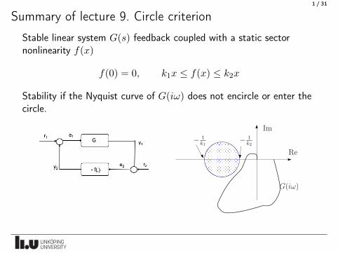
Summary of lecture 9. Circle criterionStable linear system G(s) feedback coupled with a static sector

nonlinearity f(x)

f(0) = 0, k1x f(x) k2x

Stability if the Nyquist curve of G(i!) does not encircle or enter the

circle.

Re

Im

� 1k1

� 1k2

G(i!)

2 / 31

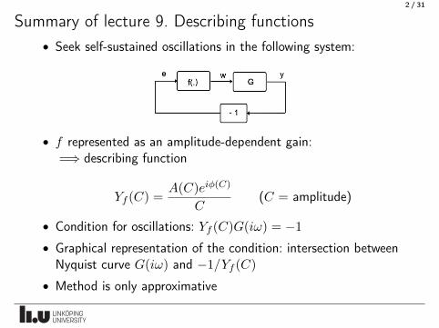
Summary of lecture 9. Describing functions• Seek self-sustained oscillations in the following system:

• f represented as an amplitude-dependent gain:

=) describing function

Yf (C) =A(C)ei�(C)

C(C = amplitude)

• Condition for oscillations: Yf (C)G(i!) = �1

• Graphical representation of the condition: intersection between

Nyquist curve G(i!) and �1/Yf (C)

• Method is only approximative

17µmemit cycle hs%YEaa

3 / 31

Amplitude stability of oscillationsWhat happens if the oscillation is perturbed (e.g. disturbance)?

• Intersection � 1Yf (C) = G(i!) can be thought as the point �1 of

the Nyquist plot of a linear system =) “critical point”

• The direction of the arrow indicates how the value of �1/Yf (C)changes when the amplitude C grows

Re

Im

<latexit sha1_base64="BfN/h9stHIQ9bj62w/Mko+Eekfc=">AAAB+nicbVDLSsNAFL2pr1pfqS7dDBahLiyJiLosduOygn1IG8JkOmmHTh7MTJQS8yluXCji1i9x5984bbPQ1gMXDufcy733eDFnUlnWt1FYWV1b3yhulra2d3b3zPJ+W0aJILRFIh6Jrocl5SykLcUUp91YUBx4nHa8cWPqdx6okCwK79Qkpk6AhyHzGcFKS65ZPu37ApPUztJ71682TjLXrFg1awa0TOycVCBH0zW/+oOIJAENFeFYyp5txcpJsVCMcJqV+omkMSZjPKQ9TUMcUOmks9MzdKyVAfIjoStUaKb+nkhxIOUk8HRngNVILnpT8T+vlyj/yklZGCeKhmS+yE84UhGa5oAGTFCi+EQTTATTtyIywjoKpdMq6RDsxZeXSfusZl/UrNvzSv06j6MIh3AEVbDhEupwA01oAYFHeIZXeDOejBfj3fiYtxaMfOYA/sD4/AE2kZNS</latexit>

� 1

Yf (C)

<latexit sha1_base64="MAw2gtFjR58F758TUhFyKs3/37A=">AAAB8nicbVDLSgNBEJz1GeMr6tHLYBDiJeyKqMegBz1GMA/YLGF2MpsMmccy0yuEkM/w4kERr36NN//GSbIHTSxoKKq66e6KU8Et+P63t7K6tr6xWdgqbu/s7u2XDg6bVmeGsgbVQpt2TCwTXLEGcBCsnRpGZCxYKx7eTv3WEzOWa/UIo5RFkvQVTzgl4KTwrsJxR0vWJ2fdUtmv+jPgZRLkpIxy1Lulr05P00wyBVQQa8PATyEaEwOcCjYpdjLLUkKHpM9CRxWRzEbj2ckTfOqUHk60caUAz9TfE2MirR3J2HVKAgO76E3F/7wwg+Q6GnOVZsAUnS9KMoFB4+n/uMcNoyBGjhBquLsV0wExhIJLqehCCBZfXibN82pwWfUfLsq1mzyOAjpGJ6iCAnSFauge1VEDUaTRM3pFbx54L9679zFvXfHymSP0B97nDwt9kHM=</latexit>

G(i!)

Stable oscillation

G- Cc e co : MYOfc conure ofG

encircles the " Coronae

pooed"- 1-

Year>

a TEE•Coq ← c. → saga of du s 026 .

To -s deeper Rede ofthee a seedgrow

asc-s Ce

C = Cz > co : Wen encirclement

→ Snafu ofstab .→ sempre tede decreases

4 / 31

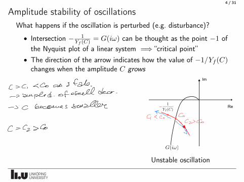
Amplitude stability of oscillationsWhat happens if the oscillation is perturbed (e.g. disturbance)?

• Intersection � 1Yf (C) = G(i!) can be thought as the point �1 of

the Nyquist plot of a linear system =) “critical point”

• The direction of the arrow indicates how the value of �1/Yf (C)changes when the amplitude C grows

Re

Im


� 1

Yf (C)


G(i!)

Unstable oscillation

C = C ,eco ⇒ s fats

.

→ anper d. ofoseell dear .

-S C becomes smallerc, • G.cz>G

C = Cz > Co \I

5 / 31

Amplitude stability of oscillationsWhat happens if G(i!) and �1/Yf (C) do not intersect each other?

Re

Im


� 1

Yf (C)


G(i!)

Re

Im


� 1

Yf (C)


G(i!)

Vanishing oscillation Unbounded growing oscillations

* the

6 / 31

Lecture 10

Phase plane analysis

• Linear phase plane

• Nonlinear phase plane

In the book: Ch. 13

7 / 31

Phase plane• Phase space: old name for state space

• Phase plane: 2-dimensional state space

• Phase portrait: graphical way to describe phase plane

• Often we simulated x1(t) and x2(t) separately as functions of

time; here instead they are represented as a single curve

• Can be sketched using eigenvalues and eigenvectors of matrix A

• Alternatively, it can be simulated from a number of initial

conditions

• Part of the results obtained in dimension 2 can be generalized to

higher dimension

"

t÷⇒.

"

tinea

8 / 31

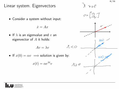
Linear system. Eigenvectors

• Consider a system without input:

x = Ax

• If � is an eigenvalue and v an

eigenvector of A it holds:

Av = �v

• If x(0) = ↵v =) solution is given by:

x(t) = ↵e�tv

I real

a- frog

or

%?no

":#AM

Casey ar . . .

,an all desoiuct

=D exist n eigenvectors un - . . ✓a

EcoleFE,

air. =D Ect) -- Zai editor .

Casey Ae . . . Au arenot distract as they may

or may not have eogeuieeoaes

EI a- 2 12=9, of multiple.2

1) J - f. Tho %) 2 blocks of tan r→ 2 eageeuee toes

2) J- [ Mf ha,] a blade of tui 2→ duly z edgewater .

• geometric Walterpliantly et ai = ne of Joedeer blades

• algebraic cuueorpliooly of Ri = sum of the awnof all Toedsee blade

of of eigenvectors for ai a geometric meltage. otar← ai of Jordan blocks

-

De Tai I - o K c

'

⇐ , as . so .

Ref ai ] so for some i =D has Ods.

ou [ai] E ont i and Thi set.

Re Enif - o

is as solvated to Jordan GCooks of duty

as stats . Cboo no Easywept . >

9 / 31

Classification of equilibrium points

The phase portrait near an equilibrium point depends on whether the

eigenvalues are real or complex, and on the sign of the real part

in doin z

O- - --•a O O

÷@ re

•

10 / 31

Distinct real eigenvalues: node• Two real, distinct and

negative eigenvalues

�1 < �2 < 0

Stable

• Two real, distinct and positive

eigenvalues

0 < �2 < �1

Unstable

Eigenvector and their ratio determine the phase portrait

- w

slow fastfast Flow× sate't

,t.ae/htrzVn(fast ) Vr Cfast)

Elstow ) uz Glow)

II's .

11 / 31

Distinct real eigenvalues: node (cont’d)

−10 −5 0 5 10−10

−8

−6

−4

−2

0

2

4

6

8

10

t=10s

x1

x2

• ”fast

eigenvector”:

�1 = �2.4

• ”slow

eigenvector”:

�2 = �0.52

12 / 31

Distinct real eigenvalues: : saddle point• Two real eigenvalues with different sign

�1 < 0 < �2

• Stable subspace: if (and only if) initial condition is exactly on

the stable eigenspace (x(0) = ↵v1) then solution is stable

- ~

ve be

on general Vz

Idol =44 the Oz

special case

XEF 2, on

-re

13 / 31

Identical eigenvalues: node• Identical eigenvalues: both real �1 = �2 = �

(1) Jordan form J =

� 10 �

�=) only 1 eigenvector

� < 0

Stable node

� > 0

Unstable node

re

14 / 31

Identical eigenvalues: star node• Identical eigenvalues: both real �1 = �2 = �

(2) Jordan form J =

� 00 �

�=) 2 independent eigenvectors

� < 0

Stable star node

� > 0

Unstable star node

15 / 31

Complex conjugate eigenvalues: focus• Complex conjugate eigenvalues �1,2 = � ± i!

� < 0

Stable focus

� > 0

Unstable focus

:# HE

16 / 31

Complex conjugate eigenvalues: focus

• Typical form of Jordan block

x =

� �!! �

�x

• Alternative form: polar coordinates

(x1 = r cos �

x2 = r sin �=)

(r = �r

� = !

• Solution is a spiral since � grows (! > 0 imaginary part)

• Distance to the origin

1. decreases if � < 0 =) asympt. stability

2. grows if � > 0 =) instability

(zeal Toedsee four )

C- talons

f- please

f is'

decreasing

in.- w

!h=t A. =D , -_ a multiple 2

.

I -_f%⇐J- Ae,-_o±iw

The = Gt dw

J - { The %) neo- c'wO as

A real

17 / 31

Purely imaginary eigenvalues: center• Purely imaginary eigenvalues �1,2 = ±i!

• In polar coordinates

(r = �r = 0

� = !=) r = const

• If � = 0 distance to the origin is constant, and the solution is a

circle around the origin

•SOable but

woe asgwp.sk.

18 / 31

Continuum of equilibria• One zero, one non-zero eigenvalues:

�1 = 0, �2 6= 0 real

�2 < 0

Stable

�2 > 0

Unstable

x. =#x x -r

ex = 0

walls pace Av -- o is economize →panda]

Yz

on

( botuotasyuyf.sk)

19 / 31

Relationship between linear and nonlinear system(near equilibrium point)

Linear system

x = Ax

has equilibrium point for x = 0

1. node, focus or saddle

point

2. center

3. continuum of equlibria

�1 = 0, �2 6= 0

Nonlinear system near x = 0

x = Ax + g(x),|g(x)||x|

x!0�! 0

has equilibrium point

1. same type

2. can be either a (stable/unstable)

focus or a center

3. can be a (stable/unstable) node,

or saddle point or a continuum of

equilibria

I -fed air dins 2

YaiI # 0 → decidable cases

Re Cai ]--o

lou decidable cases

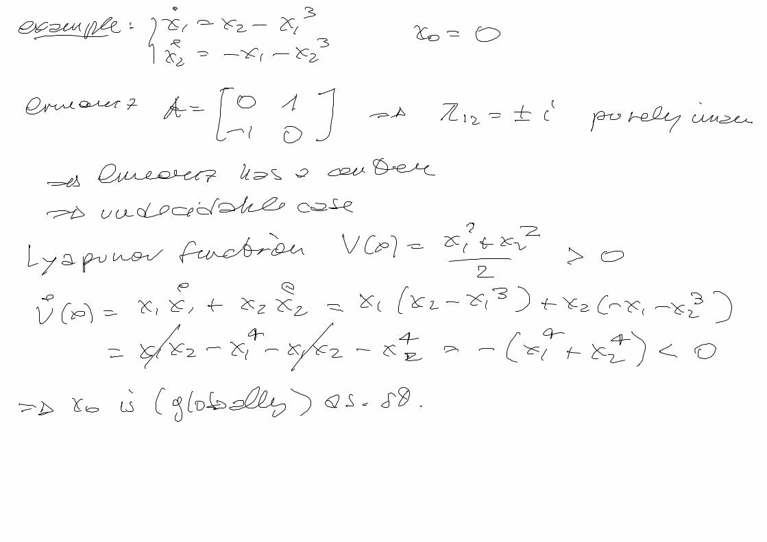
exude : foie - xz - XP Xo = O

£2 = -X, - XP

evueaiett A-- JI, to ] as Riz = I c'

purely imam

=D Omelet has acar Ieee

=D undecidable case,

Lyapunov functionVce) = xitxF- S OZ

J (e) = X ,I, t Xz £2 = Xc (K2 - 43 ) txzcnx,

-xp )= xfxz - xih-xfxz-x.dz = - (xTtxI) e o

=D Xo is ( globally) as . SO .

exe I, = Xa t x? Xo = o

E = -x, t XP

dice : A = II, I ] → undecidable case

Lyap . final : VA)=xE > o

2

V. Co) = x , xectxexz =. . .

= x Ft XF > 0

Vcd keeps growing =D diverge !=D Xo is unstable

as 2 syst with same lrueeeeitabeoii but opposer de

stability at equil

20 / 31

Phase portrait away from equilibrium points• Nonlinear second order system

x1 = f1(x1, x2)

x2 = f2(x1, x2)

• Construct the ratio of derivates

dx2

dx1=

dx2

dt

dt

dx1=

x2

x1=

f2(x1, x2)

f1(x1, x2)

• slope for (x1, x2) is

• horizontal when f2(x1, x2) = 0• vertical when f1(x1, x2) = 0

• phase plane behavior from the limit values

limx1!±1

f2(x1, x2)

f1(x1, x2), lim

x2!±1

f2(x1, x2)

f1(x1, x2)

Towerozonic agemeatsp -

*⇒µ

thorough srumleetiaesplotCee , xD

21 / 31

Example: phase plane for generator/pendulumSystem: x1 = x2

x2 = �ax2 � b sin x1

• equilibria: x0 =

±2k⇡

0

�

• linearization

A =

0 1

�b �a

�

• eigenvalues:

�1,2 = (�a ±p

a2 � 4b)/2

= � ± i!

• =) stable focus

• equilibria: x0 =

⇡ ± 2k⇡

0

�

• linearization

A =

0 1b �a

�

• eigenvalues:

�1,2 = (�a ±p

a2 + 4b)/2

�1 < 0, �2 > 0

• =) saddle point

X. = angle

} k= aug .wel

.

down up

25- stable vase .

Tl.

22 / 31

Example: phase plane for generator/pendulum

−4 −3 −2 −1 0 1 2 3 4−4

−3

−2

−1

0

1

2

3

4

• Equilibrium point in the origin is a stable focus• Equilibrium points in (±⇡, 0) are saddle points (red lines show

eigenvectors)

plot her , Eu ) "quaver

"

↳ to↳

y

t•- - • - - - ti

¢l

l

l

ll

23 / 31

Example: epidemic model

Example: epidemic model

dS

dt= �↵SI

dI

dt= ↵SI � �I

dR

dt= �I

Variables:

• S = susceptible

• I = infected

• R = removed

Parameters:

• ↵ = infectivity rate (1 < ↵ 10)

• � = removal rate (� = 1)

S,I,R > 0

(recovered + deceased)\me, .mg , ,§Rfftd§tfI=0 =D scat Ict> I

equilibria : I - O,

StR=N (25-3)=0

5- Fg equilibria : Orioles (5. I. E) set.I -- O 5th-N → continuumof

equilibria

* t. ÷:÷¥⇒÷t÷÷ :o)detente -H) --dot II o ) - idea -ashes) -o

o -B d

Nez = O 23=25-B

if 25- B > o =D 57 Bz ⇒ Az so ⇒ unstable

if 45 -Bee ⇒ azero ⇒ undecidable case

Ro = reproductive 224in = IB

dff -- ASI-BI - (Fs s -DRI = B. (Ros - 1) IIf Ro > Is =D TIE 20 =D rid of infected gum,

If Ro est as IIe To ⇒ rioter feeEad desires

Carta dug spreading-decrease 2 ( social distancing , vaccine)- aware- se p ( drugs>

phase portrait in ⇐II place

÷÷.

%⇒"flattening the curve

"← I

24 / 31

Example: epidemic model• low infectivity rate: ↵ = 1.5

0 5 10 15 20

time

0

0.2

0.4

0.6

0.8

1

S

I

R

0 0.2 0.4 0.6 0.8 1

S

0

0.2

0.4

0.6

0.8

1

I

• high infectivity rate: ↵ = 5

0 5 10 15 20

time

0

0.2

0.4

0.6

0.8

1

S

I

R

0 0.2 0.4 0.6 0.8 1

S

0

0.2

0.4

0.6

0.8

1

I

FELL

25 / 31

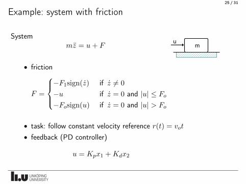
Example: system with friction

System

mz = u + F mu

• friction

F =

8><

>:

�F1sign(z) if z 6= 0

�u if z = 0 and |u| Fo

�Fosign(u) if z = 0 and |u| > Fo

• task: follow constant velocity reference r(t) = vot

• feedback (PD controller)

u = Kpx1 + Kdx2

26 / 31

Example: system with friction• state variables x1 = error = r � z

x2 = velocity error = x1

• closed loop state space model

x1 = x2

x2 =1

m(�u � F ) =

1

m(�Kpx1 � Kdx2 � F )

• parameters: vo = 1, m = 1, Fo = 1.5, F1 = 1, Kp = 1

• piece-wise linear system: switching between linear modes

x1 = x2

x2 =

8><

>:

�x1 � Kdx2 + sign(1 � x2) if x2 6= 1

0 if x2 = 1, |x1 + Kd| 1.5

�x1 � Kdx2 + 1.5sign(x1 + Kd) if x2 = 1, |x1 + Kd| > 1.5

27 / 31


• 3 important regions in state space

(a) if x2 > 1

x1 = x2

x2 = �x1 � Kdx2 � 1

(b) if x2 < 1

x1 = x2

x2 = �x1 � Kdx2 + 1

(c) if x2 = 1 and |x1 + Kd| 1.5

x1 = x2

x2 = 0

(d) if x2 = 1 and |x1 + Kd| > 1.5(not important: immediately switches to (a) or (b))

28 / 31


• Equilibria analysis

(a) if x2 > 1 (x1 = �1

x2 = 0=) the equil is outside the region itself

(b) if x2 < 1 (x1 = 1

x2 = 0

(c) if x2 = 1 and |x1 + Kd| 1.5 =) no equilibrium

• Linearization (for (a) and (b))

A =

0 1

�1 �Kd

�=) �1,2 = �Kd

2± 1

2

qK2

d � 4

29 / 31


�1,2 = �Kd

2± 1

2

qK2

d � 4

Possible cases for the equilibrium in (a) and (b)

1. Kd = 0 (i.e. P controller): �1,2 = ±i =) center

2. 0 < Kd < 2 : �1,2 complex conjugate =) stable focus

3. Kd = 2 : �1,2 = �Kd2 =) real, negative eigenval of multipl. 2

4. Kd > 2 : �1,2 =) two distinct, real, negative eigenvalues

30 / 31


Kd = 0.1 Kd = 0.02

31 / 31

Two examples with three state variables

Examples of generalization to higher dimension

Stable ”focus node”

(focus + one real eigenvalue)

−1−0.5

00.5

1

−1−0.5

00.5

10

0.2

0.4

0.6

0.8

1

Stable equilibrium with 3 distinct

real eigenvalues

(generalization of 2 distinct real

eigenvalues case)

0

0.2

0.40.6

0.8

1

0

0.5

1

0

0.2

0.4

0.6

0.8

1

TSRT09 Control Theory 2021,Lecture 10

www.liu.se

tsrt09 – control theory

Documents