Truncated skew-normal distributions: moments, estimation by

weighted moments and application to climatic data

by C. Flecher1,2, D. Allard1 and P. Naveau2

1 Biostatistics and Spatial Processes,

INRA, Agroparc 84914 Avignon, France2 Laboratoire des Sciences du Climat et de l'Environnement,

CNRS Gif-sur-Yvette, France

Running title: Truncated skew-normal distributions

Abstract In this paper we derive an expression of the mth order moments and some weighted mo-

ments of truncated skew-normal distributions. We link these formulas to previous results for trun-

cated distributions and non truncated skew-normal distributions. Methods to estimate skew-normal

parameters using weighted moments are proposed and compared to other classical techniques. In a

second step we propose to model the distribution of relative humidity with a truncated skew-normal

distribution.

Key words: Truncated skew-normal distributions, inference methods, classical moments, weighted

moments, relative humidity.

1

1 Introduction

In many applications, the probability distribution function (pdf) of some observed variables can be

simultaneously skewed and restricted to a �xed interval. For example, variables such as pH, grades,

and humidity in environmental studies, have upper and lower physical bounds and their pdfs are

not necessarily symmetric within these bounds. To illustrate such behaviors, Figure 1 shows the

histograms per season and the estimated pdfs of daily relative humidity measurements made in

Toulouse (France) from 1972 to 1999.

Dec−Jan−Feb

H (%)

Den

sity

0 20 40 60 80 100

0.00

0.01

0.02

0.03

0.04

0.05

0.06

Mar−Apr−May

H (%)

Den

sity

0 20 40 60 80 100

0.00

0.01

0.02

0.03

0.04

0.05

0.06

Jun−Jul−Aug

H (%)

Den

sity

0 20 40 60 80 100

0.00

0.01

0.02

0.03

0.04

0.05

0.06

Sep−Oct−Nov

H (%)

Den

sity

0 20 40 60 80 100

0.00

0.01

0.02

0.03

0.04

0.05

0.06

Figure 1: Histograms and estimated densities of daily relative humidity measurements made in

Toulouse (France) from 1972 to 1999. Each panel corresponds to a season.

All observations belong to the interval [0, 100] and skewness is apparent, especially during the Spring

and Fall seasons. There are many strategies available to model such skewed and bounded data.

In this paper our approach is to conceptually view such observations as truncated measurements

originating from a �exible skewed distribution. More precisely we assume that the truncation bounds

are known and we focus on the following skew-normal pdf de�ned by Azzalini (1985)

fµ,σ,λ(x) =2σφ

(x− µσ

)Φ(λx− µσ

), (1)

where µ ∈ R, σ > 0 and λ ∈ R represent the location, scale and shape parameters, respectively.

The notations φ and Φ correspond to the pdf and the cumulative distribution function (cdf) of the

standard normal distribution, respectively. The skew-normal distribution (1) can be obtained from

a bivariate Gaussian random vector, by conditioning one component on the second one being above

(or below) a given threshold (Azzalini, 1985). The notation X ∼ SN(µ, σ, λ) represents a random

variable, X, following (1) and Fµ,σ,λ denotes its cdf. The particular case λ = 0 corresponds to the

classical normal distribution with mean µ and variance σ2. In the following, the pdf and the cdf

of a SN(0, 1, λ) are simply denoted fλ and Fλ. In this context our main objective is to propose

and study a novel method-of-moments approach for estimating the parameters of (1) in presence of

truncation.

2

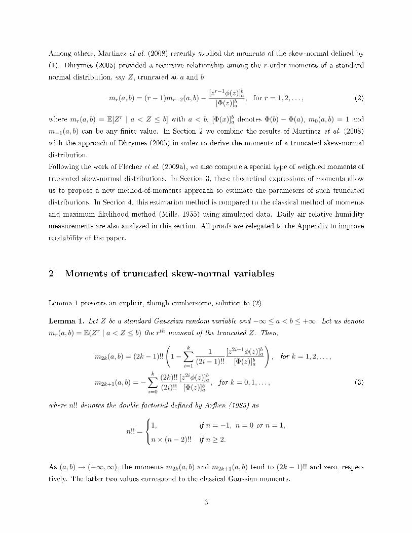
Among others, Martinez et al. (2008) recently studied the moments of the skew-normal de�ned by

(1). Dhrymes (2005) provided a recursive relationship among the r-order moments of a standard

normal distribution, say Z, truncated at a and b

mr(a, b) = (r − 1)mr−2(a, b)− [zr−1φ(z)]ba[Φ(z)]ba

, for r = 1, 2, . . . , (2)

where mr(a, b) = E[Zr | a < Z ≤ b] with a < b, [Φ(x)]ba denotes Φ(b) − Φ(a), m0(a, b) = 1 and

m−1(a, b) can be any �nite value. In Section 2 we combine the results of Martinez et al. (2008)

with the approach of Dhrymes (2005) in order to derive the moments of a truncated skew-normal

distribution.

Following the work of Flecher et al. (2009a), we also compute a special type of weighted moments of

truncated skew-normal distributions. In Section 3, these theoretical expressions of moments allow

us to propose a new method-of-moments approach to estimate the parameters of such truncated

distributions. In Section 4, this estimation method is compared to the classical method-of-moments

and maximum likelihood method (Mills, 1955) using simulated data. Daily air relative humidity

measurements are also analyzed in this section. All proofs are relegated to the Appendix to improve

readability of the paper.

2 Moments of truncated skew-normal variables

Lemma 1 presents an explicit, though cumbersome, solution to (2).

Lemma 1. Let Z be a standard Gaussian random variable and −∞ ≤ a < b ≤ +∞. Let us denote

mr(a, b) = E(Zr | a < Z ≤ b) the rth moment of the truncated Z. Then,

m2k(a, b) = (2k − 1)!!

(1−

k∑i=1

1(2i− 1)!!

[z2i−1φ(z)]ba[Φ(z)]ba

), for k = 1, 2, . . . ,

m2k+1(a, b) = −k∑i=0

(2k)!!(2i)!!

[z2iφ(z)]ba[Φ(z)]ba

, for k = 0, 1, . . . , (3)

where n!! denotes the double factorial de�ned by Arfken (1985) as

n!! =

1, if n = −1, n = 0 or n = 1,

n× (n− 2)!! if n ≥ 2.

As (a, b) → (−∞,∞), the moments m2k(a, b) and m2k+1(a, b) tend to (2k − 1)!! and zero, respec-

tively. The latter two values correspond to the classical Gaussian moments.

3

We now introduce the truncated skew-normal distribution as a truncation of the skew-normal dis-

tribution in 1. Its pdf is

fµ,σ,λ(x | a < X ≤ b) =

1

[Fµ,σ,λ(x)]bafµ,σ,λ(x), if a < x ≤ b,

0 otherwise,(4)

where X ∼ SN(µ, σ, λ) and −∞ ≤ a < b ≤ +∞ represents the range of the truncation. Let us

consider the simple case (µ, σ) = (0, 1).

Proposition 1. Let X be a SN(0, 1, λ). Let us denote sλ,r(u, v) = E[Xr | u < X ≤ v] with u < v

the rth moment of the truncated variable. The following recursive relationship holds,

sλ,r(u, v) = (r − 1)sλ,r−2(u, v) + rλ,r(u, v), for r = 1, 2, . . . , (5)

where sλ,0(u, v) = 1 and sλ,−1 can be any �nite value,

rλ,r(u, v) = − [xr−1fλ(x)]vu[Fλ(x)]vu

+2√2π

λ

λr∗

[Φ(λ∗x)]vu[Fλ(x)]vu

mr−1(λ∗u, λ∗v),

where λ∗ = (1 + λ2)1/2. From (5), we can derive

sλ,2p(u, v) = (2p− 1)!! +p∑

k=1

(2p− 1)!!(2k − 1)!!

rλ,2k(u, v), with p = 1, 2, . . . , (6)

sλ,2p+1(u, v) =p∑

k=0

(2p)!!(2k)!!

rλ,2k+1(u, v), with p = 0, 1, . . . . (7)

Martinez's et al. (2008) results can be viewed as limiting cases of (6) and (7)

lim(u,v)→(−∞,+∞)

sλ,2p(u, v) = (2p− 1)!!, with p = 0, 1, . . . ,

lim(u,v)→(−∞,+∞)

sλ,2p+1(u, v) =2√2π

p∑k=0

(2p)!!(2k)!!

(2k − 1)!!λ

(1 + λ2)k+1/2, with p = 0, 1, . . . .

Equalities (6) and (7) tell us that odd (respectively even) moments of truncated skew-normal distri-

butions can be interpreted as linear combinations of even (respectively odd) moments of the normal

distribution truncated at λ∗u and λ∗v. If λ = 0, Equation (5) and Proposition 1 are equivalent

to the recursive equation provided in Dhrymes (2005) and Lemma 1, respectively. The restricting

condition (µ, σ) = (0, 1) can be easily removed and leads to the following proposition.

Proposition 2. Let X ∼ SN(µ, σ, λ). Then, we have

E[Xm | a < X ≤ b] =m∑r=0

Crmµm−rσrsλ,r(u, v). (8)

where u = (a−µ)/σ, v = (b−µ)/σ, Crm =

(m

r

)is a binomial coe�cient and sλ,r(u, v) is de�ned

in Proposition 1.

4

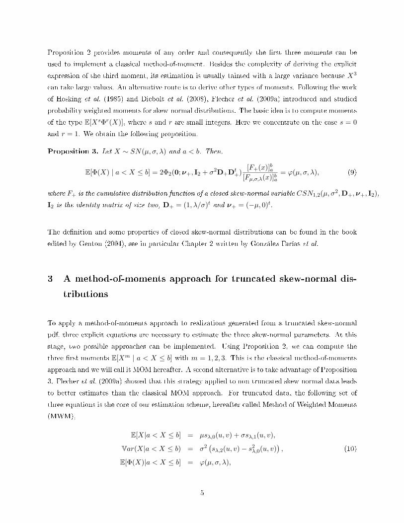
Proposition 2 provides moments of any order and consequently the �rst three moments can be

used to implement a classical method-of-moment. Besides the complexity of deriving the explicit

expression of the third moment, its estimation is usually tainted with a large variance because X3

can take large values. An alternative route is to derive other types of moments. Following the work

of Hosking et al. (1985) and Diebolt et al. (2008), Flecher et al. (2009a) introduced and studied

probability weighted moments for skew-normal distributions. The basic idea is to compute moments

of the type E[XsΦr(X)], where s and r are small integers. Here we concentrate on the case s = 0

and r = 1. We obtain the following proposition.

Proposition 3. Let X ∼ SN(µ, σ, λ) and a < b. Then,

E[Φ(X) | a < X ≤ b] = 2Φ2(0; ν+, I2 + σ2D+Dt+)

[F+(x)]ba[Fµ,σ,λ(x)]ba

= ϕ(µ, σ, λ), (9)

where F+ is the cumulative distribution function of a closed skew-normal variable CSN1,2(µ, σ2,D+,ν+, I2),

I2 is the identity matrix of size two, D+ = (1, λ/σ)t and ν+ = (−µ, 0)t.

The de�nition and some properties of closed skew-normal distributions can be found in the book

edited by Genton (2004), see in particular Chapter 2 written by González-Farías et al.

3 A method-of-moments approach for truncated skew-normal dis-

tributions

To apply a method-of-moments approach to realizations generated from a truncated skew-normal

pdf, three explicit equations are necessary to estimate the three skew-normal parameters. At this

stage, two possible approaches can be implemented. Using Proposition 2, we can compute the

three �rst moments E[Xm | a < X ≤ b] with m = 1, 2, 3. This is the classical method-of-moments

approach and we will call it MOM hereafter. A second alternative is to take advantage of Proposition

3. Flecher et al. (2009a) showed that this strategy applied to non-truncated skew-normal data leads

to better estimates than the classical MOM approach. For truncated data, the following set of

three equations is the core of our estimation scheme, hereafter called Method of Weighted Moments

(MWM),

E[X|a < X ≤ b] = µsλ,0(u, v) + σsλ,1(u, v),

Var(X|a < X ≤ b) = σ2(sλ,2(u, v)− s2λ,0(u, v)

), (10)

E[Φ(X)|a < X ≤ b] = ϕ(µ, σ, λ),

5

with u = (a − µ)/σ, v = (b − µ)/σ and sλ,r(u, v) is de�ned in Proposition 1. The name �Method

of Weighted Moments� can be justi�ed by recalling that the system de�ned by (10) stems from the

�weighted moments� E(XrΦs(X)|a < X ≤ b) with (r, s) = (1, 0), (r, s) = (2, 0) and (r, s) = (0, 1).

To estimate the parameters, we used the following scheme:

• Compute the empirical moments corresponding to E[X | a < X ≤ b],Var(X | a < X ≤ b) andE[Φ(X) | a < X ≤ b],

• solve (10) for (µ, σ, λ) using nlminb function in R.

The complexity of the equations, in particular the last equation related to the weighted moment,

does not allow us to obtain distributional results for the estimators (µ̂, σ̂, λ̂). The performance of

this estimation scheme must therefore be assessed by simulation.

Figure 2 shows how E[X3 | a < X ≤ b] (right panel) and E[Φ(X) | a < X ≤ b] (left panel) vary

as functions of λ, when (µ, σ) = (0, 1) with 10% or 20% of left truncation. Boxplots have been

obtained from 1000 replicates of the empirical moments, each one being computed on a sample of

500 truncated skew-normal random variables. Clearly, the estimates of E[Φ(X) | a < X ≤ b] are

much less dispersed those of E[X3 | a < X ≤ b], specially for low to moderate values of λ. Both

curves �atten out as λ reaches large values. It is thus very di�cult to estimate large values of

λ, say λ ≥ 4. Similar results have also been obtained with di�erent truncation schemes and/or

truncation intensities, or without any truncation at all (see the next section for a precise de�nition

of truncation intensity). These are good indications that the weighted moment should be preferred

to the third moment, see also Tables 1 and 2 below.

4 Data analysis

4.1 Simulations

To assess our inference method we simulated 1000 vectors of size 500 of independent replicates, using

the rsn function of the R package sn (Azzalini, 2009). We considered three values for the shape

parameter λ ∈ {1, 2, 4}, corresponding to respectively low, medium and high levels of skewness.

Because λ plays a symmetrical role, we restricted ourselves to positive values for λ; λ = 0 corresponds

to absence of skewness. Note also that λ = 4 is located in a relatively �at area of the curve

E[Φ(X)|a < X ≤ b](λ), i.e. di�erent large values of λ give a similar weighted moment. Since

6

1 2 4

0.40

0.45

0.50

0.55

0.60

0.65

0.70

0.75

(a)

λλ

E[ΦΦ

(X)]

1 2 4

0.40

0.45

0.50

0.55

0.60

0.65

0.70

0.75

10%

20%

1 2 4−

0.30

−0.

25−

0.20

−0.

15−

0.10

−0.

050.

000.

05

(b)

λλ

Sλλ,

3(ξξ 1

,ξξ2)

1 2 4−

0.30

−0.

25−

0.20

−0.

15−

0.10

−0.

050.

000.

05

10%

20%

Figure 2: Theoretical and empirical moments of E[Φ(X) | a < X ≤ b] and E[X3 | a < X ≤ b] as

a function of λ. Boxplots are computed on 1000 samples of size 500 of truncated SN(0, 1, λ) with

λ ∈ {1, 2, 4} and 10% and 20% left truncations.

Table 1: Bias and Mean-Square-Error (MSE) for the MWM, MOM and MLE (Maximum Likelihood Esti-

mates) approaches obtained from 1000 replicates of size 500 for left or right truncation with intensity 20%

and parameters (µ, σ, λ) = (0, 1, 2).

MWM MOM MLE

Bias MSE Bias MSE Bias MSE

µ̂ 0.033 0.027 0.106 0.063 0.107 0.042

Left truncation σ̂ −0.024 0.007 −0.033 0.010 −0.031 0.010

λ̂ −0.434 1.143 1994 8.5 107 46.1 5.7 105

µ̂ 0.059 0.033 0.033 0.038 0.044 0.042

Right truncation σ̂ 0.004 0.159 0.107 0.543 0.063 0.163

λ̂ −0.003 1.806 0.372 5.546 0.213 2.214

left and right truncation do not play a symmetrical role, we considered left, right and bilateral

truncation. The intensity of the truncation is de�ned as the probability that the non truncated

7

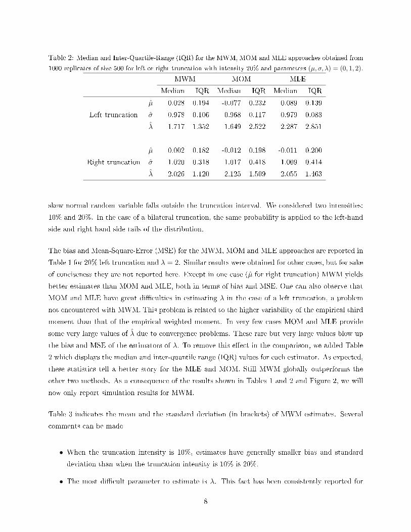
Table 2: Median and Inter-Quartile-Range (IQR) for the MWM, MOM and MLE approaches obtained from

1000 replicates of size 500 for left or right truncation with intensity 20% and parameters (µ, σ, λ) = (0, 1, 2).

MWM MOM MLE

Median IQR Median IQR Median IQR

µ̂ 0.028 0.194 -0.077 0.232 0.089 0.139

Left truncation σ̂ 0.978 0.106 0.968 0.117 0.979 0.083

λ̂ 1.717 1.352 1.649 2.522 2.287 2.851

µ̂ 0.002 0.182 -0.012 0.198 -0.011 0.200

Right truncation σ̂ 1.020 0.318 1.017 0.418 1.009 0.414

λ̂ 2.026 1.120 2.125 1.509 2.055 1.463

skew-normal random variable falls outside the truncation interval. We considered two intensities:

10% and 20%. In the case of a bilateral truncation, the same probability is applied to the left-hand

side and right-hand side tails of the distribution.

The bias and Mean-Square-Error (MSE) for the MWM, MOM and MLE approaches are reported in

Table 1 for 20% left truncation and λ = 2. Similar results were obtained for other cases, but for sake

of conciseness they are not reported here. Except in one case (µ̂ for right truncation) MWM yields

better estimates than MOM and MLE, both in terms of bias and MSE. One can also observe that

MOM and MLE have great di�culties in estimating λ in the case of a left truncation, a problem

not encountered with MWM. This problem is related to the higher variability of the empirical third

moment than that of the empirical weighted moment. In very few cases MOM and MLE provide

some very large values of λ̂ due to convergence problems. These rare but very large values blow up

the bias and MSE of the estimators of λ. To remove this e�ect in the comparison, we added Table

2 which displays the median and inter-quantile range (IQR) values for each estimator. As expected,

these statistics tell a better story for the MLE and MOM. Still MWM globally outperforms the

other two methods. As a consequence of the results shown in Tables 1 and 2 and Figure 2, we will

now only report simulation results for MWM.

Table 3 indicates the mean and the standard deviation (in brackets) of MWM estimates. Several

comments can be made

• When the truncation intensity is 10%, estimates have generally smaller bias and standard

deviation than when the truncation intensity is 10% is 20%.

• The most di�cult parameter to estimate is λ. This fact has been consistently reported for

8

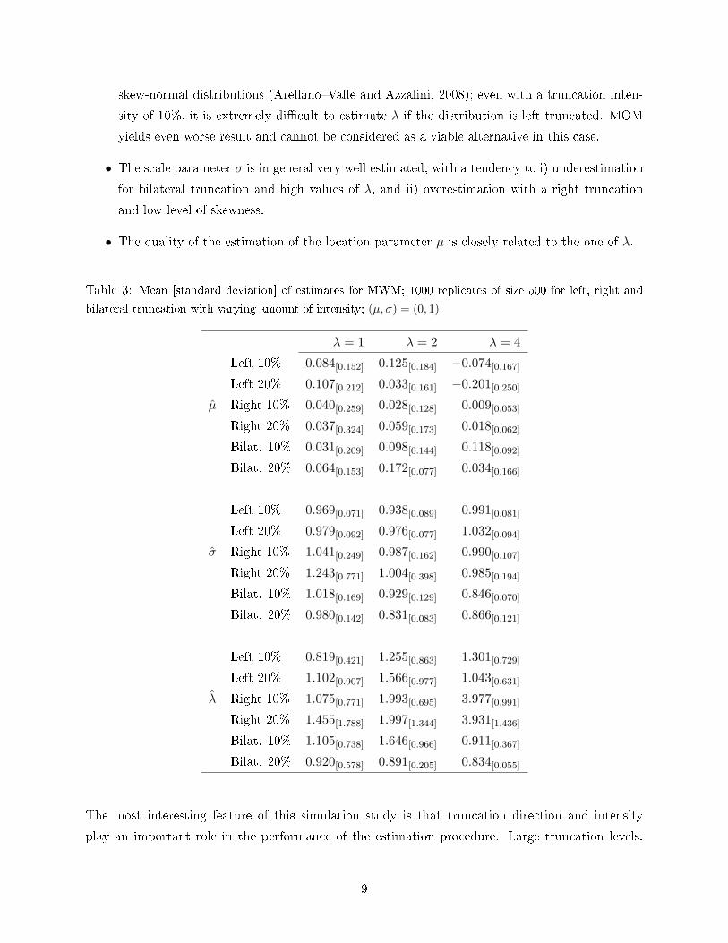
skew-normal distributions (Arellano�Valle and Azzalini, 2008); even with a truncation inten-

sity of 10%, it is extremely di�cult to estimate λ if the distribution is left truncated. MOM

yields even worse result and cannot be considered as a viable alternative in this case.

• The scale parameter σ is in general very well estimated; with a tendency to i) underestimation

for bilateral truncation and high values of λ, and ii) overestimation with a right truncation

and low level of skewness.

• The quality of the estimation of the location parameter µ is closely related to the one of λ.

Table 3: Mean [standard deviation] of estimates for MWM; 1000 replicates of size 500 for left, right and

bilateral truncation with varying amount of intensity; (µ, σ) = (0, 1).

λ = 1 λ = 2 λ = 4

Left 10% 0.084[0.152] 0.125[0.184] −0.074[0.167]

Left 20% 0.107[0.212] 0.033[0.161] −0.201[0.250]

µ̂ Right 10% 0.040[0.259] 0.028[0.128] 0.009[0.053]

Right 20% 0.037[0.324] 0.059[0.173] 0.018[0.062]

Bilat. 10% 0.031[0.209] 0.098[0.144] 0.118[0.092]

Bilat. 20% 0.064[0.153] 0.172[0.077] 0.034[0.166]

Left 10% 0.969[0.071] 0.938[0.089] 0.991[0.081]

Left 20% 0.979[0.092] 0.976[0.077] 1.032[0.094]

σ̂ Right 10% 1.041[0.249] 0.987[0.162] 0.990[0.107]

Right 20% 1.243[0.771] 1.004[0.398] 0.985[0.194]

Bilat. 10% 1.018[0.169] 0.929[0.129] 0.846[0.070]

Bilat. 20% 0.980[0.142] 0.831[0.083] 0.866[0.121]

Left 10% 0.819[0.421] 1.255[0.863] 1.301[0.729]

Left 20% 1.102[0.907] 1.566[0.977] 1.043[0.631]

λ̂ Right 10% 1.075[0.771] 1.993[0.695] 3.977[0.991]

Right 20% 1.455[1.788] 1.997[1.344] 3.931[1.436]

Bilat. 10% 1.105[0.738] 1.646[0.966] 0.911[0.367]

Bilat. 20% 0.920[0.578] 0.891[0.205] 0.834[0.055]

The most interesting feature of this simulation study is that truncation direction and intensity

play an important role in the performance of the estimation procedure. Large truncation levels,

9

especially for bilateral and left truncation when the shape parameter is large, diminish the overall

estimation quality.

In some cases, identi�ability issues arise. Consider for example a one-sided truncation at a = 0 (i.e.

the density is equal to zero for negative values). Because a skew-normal distribution with in�nite

shape parameter λ is nothing but a standard normal distribution truncated at zero, the two sets of

parameters (µ = 0, σ = 1, λ = 0, a =∞) and (µ = 0, σ = 1, λ =∞, a = 0) lead to the same density.

In this case these two sets of parameter are undistinguishable. This is a special degenerate case, but

obviously, some situations can lead to di�erent sets of parameters with very similar distributions.

Consider for example the estimation of a SN(0, 1, 2) with 20% left truncation. The estimates are

plotted in Figure 3. Values of λ̂ ranges from 0.1 to 5.5, with a mean equal to 1.5. Figure 3a shows

that the distribution of λ̂ is bimodal, corresponding to two populations of estimates (µ̂, σ̂, λ̂) of

comparable size (see Table 4).

λλ̂

Fre

quen

cy

0 1 2 3 4

050

100

150

200

●●

●

●

●

●●

●●

●

●

●●

●

●●

●

●

●

●

●

●

●

●

●

●

●

●

●

●

●●

●

●

● ●

●

●

●

●

●

●

●

●

●

●

●

●●●

●

●

●

●

●

●

●

●

●

●

●●

●

●

●

●

●

●

●

●

●

●

●

● ●

●

●

●

●

●

●

●

●

●

●

●●

●

●

●

●

●

●

●

●

●

●

●

●

●

●

●

●

●

●

●

●

●

●

●

●

●

●

●

●

●

●

●●

●

●

●

●

●

●●

●

●●

●

●

●●

●

●

●

●

●

●

●

● ●

●

●

●

●

●

●

●

●●

●

● ●●●

●

●

●

●

● ●●

●

●

●

●●

●

●

●

●

●

●

●

●●

●

●

●

●

●

●●

●

●

●

●●

●

●

●●

●

●

●

●

●

●

●

●

●

●

●

●

●

●●

●●

●

●

●

●

●

●

●

●

●

●

●

●●

●

●

●

●

●

●

●

●

●

●

●

●●

●

●

●

●

●

●

●

●●

●

●

●

●

●●

●

●

●

●

●

●

●

●

●

●

●

●

●

●

●

● ●

●

●

●

●

●

● ●●

●

●

●

●

●●

●

●●

●

●

●

●

●

●

●

●

●

●

●

●

●

●

●

●

●

●

●

●

●

●

●

●

●

●

●

●

●

●

●

●

●

●

●

●

●

●

●

●

●

●

●

●

●

●

●

●

●

●

●

●

●

●

●

●●

●●●

●

●

●

●●

●

●

●

●

●

●●

●

●

●

●

●

●

●

●

●

●

●

●

●

●

●

●

●

●

●

●

●

●

●

●

●

●

●

●

●

●

●

●

●

●

●

●

●

●

●

●

●

●● ●

●

●

●

●

●

●

●

●

●

●

●

●

●●

●

●

●

●

●

●

●

●

●

●

●

●

●

●

●

●

●

●

●

●

●

●

●

●

●●

●

●

●

●

●

●

●

●

●

●

●

●

●

●

●

●

●

●

●●

●

●

●

●

●

●

●

●

●

●

●

●

●

●

●

●

●

●

●

●

●

●●

●

●

●

●

●

●

●

●

●●

●

●

●

●●

●

●

●

●

●

●

●

●

●

● ●

●

●

●

●

●

●

●

●

●

●

●●

●

●

●

●

●

●

●

●

●

●

●

●

●

●

●

●

●●

●

● ●

●

●

●

●●

●

●

●

●●

●

●

●

●

●

●

●

●

●

●

●

●

●

●

●

●

●

●

●

●

●

●

●

●

●

●

●

●

●

●

●

●

●

●

●

●

●

●

●●

●●●

●

●

●

●

●

●

●

●

●

●

● ●

●

● ●

●

●●

●●

●

●

●●

●●

●

●

●

●

●

●

●

●

●

●

●●

●

●

●

●

●

●

●

●

●

●

●

●●

●

●

●

●

●●

●

●

●

●

●

●

●

●

●

●

●

●

●

●

●

●

●●●

●

●

●

●●

●

●

●●

●

●

●

●

●

●

●

●●

●

●

●

●

●

●

●

●

●●●

●

●

●●

●

●

●

●●

●

●

●

●

●

●●

●●

●

●

●

●

●

●

●

●●

●

●

●●

●

●

●

●

●

●

●

●

●

●

●●

●

●

●

●

●

●●

●

●●

●

●

●

●

●

●

●

●

●

●

●

●

●

●

●

●

●

●

●

●

●

●

●

●

●

●

●

●

●

●

●

●

●

●

●

●

●

●

●

●

●

●

●

●

●

●

●

●

●

●

●

●●

●

●

●

●

●

●

●●

●

●●

●●

●●

●

●

●

●

●

●

●

●

●

●

●

●

●

●

● ●

●

●

●

●

●

●

●

●

●

●

●

●●

●

●

●

●

●

●

●

●

●

●

●●

●

●

●●

●

●

●●

●

●

●

●●

●

●

●

●

●●

●

●●

●

●

●

●●

●

●

●

●

●

●●

●

●

●

●

●

●

●

●

●

●

●

●

●

●

●

●

●

●

●

●

●

●

●

●

●

●

●

●

●

●

●●

●

●

●

●

●● ●

●

●

●

●

●

●

●

●●

●

●

●

●

●

●

●

●

●

●

●

●

●

●

●

●

●

●

●

●●

●

●

●

●

●

●●

●

●

●

●

●

●

●●

●

●

●

●

●

●

●

●

●

●

●

●

●

●

●

●

●

●

●

−0.5 0.0 0.5

0.8

0.9

1.0

1.1

1.2

1.3

µµ̂

σσ̂

Figure 3: Estimates of (µ, σ, λ) computed from 1000 samples of size 500 of truncated SN (0, 1, 4)

with a 10% left truncation.

Figure 4 displays the true density and two other densities corresponding to the two populations.

This �gure clearly indicates that the three densities are very close. They di�er mainly near the

truncation threshold.

10

−0.5 0.0 0.5 1.0 1.5 2.0 2.5 3.0

0.0

0.2

0.4

0.6

dens

ity

SN(0,1,2)SN(0.09,0.94,0.69)SN(−0.01,1.01,2.3)

Figure 4: Black solid line: 20% left truncated SN(0,1,2); grey pointed line: typical density of group

#1, SN(0.09,0.94,0.69); grey dashed line: typical density of group #2, SN(-0.01,1.01,2.3).

This example illustrates two important facts. Firstly MOM has greater di�culties than MWM for

estimating the parameters since the third moment E[X3 | a < X ≤ b] is very sensitive to large valuesof X, see Table 1. Secondly, if λ is positive, the parameters are di�cult to estimate in presence of

a left truncation, but there are no particular problems for right truncations, see Table 3. It is the

opposite when λ is negative.

4.2 Daily relative humidity measurements

The relative humidity of an air-water mixture is de�ned as the ratio of the partial pressure of the

water vapor in the mixture to the saturated vapor pressure of water at a prescribed temperature

(Perry, 2007). This quantity is normally expressed as a percentage and is thus restricted to the

interval [0, 100]. The data set considered here consists of daily measurements of relative humidity

recorded by the INRA weather station located in Toulouse, South of France, between 1972 and

1999. In temperate regions, relative humidity is always much larger than 0; truncation at 100

is the only truncation visible on the experimental histograms. We will therefore consider right

11

Table 4: Mean [standard deviation] of the estimates of a SN(0, 1, 2) with 20% left truncation, when

clustered in two populations.

Group # 1 Group # 2

N 463 537

µ̂ 0.085[0.187] −0.011[0.116]

σ̂ 0.936[0.079] 1.009[0.056]

λ̂ 0.694[0.367] 2.31[0.663]

Intensity 33.2%[7.6] 19.4%[7.3]

truncation only. To take into account the seasonality e�ect, the year is divided into four periods,

(Semenov et al., 1998; Flecher et al., 2009b): December-January-February (DJF), March-April-

May (MAM), June-July-August (JJA) and September-October-November (SON). Our goal is to

�t a truncated skew-normal distribution for each one of the four periods assuming climatological

stationarity throughout the whole period 1972-1999. The cooresponding histograms are represented

in Figure 1.

For each season, the parameters were estimated using MOM and MWM. Results are presented in

Table 5. In JJA, λ̂ is positive, and the estimates obtained with the two methods are very close,

as discussed in the previous section. For the other seasons, λ̂ is negative, i.e. we encounter the

di�cult case described in the previous section. Hence, MOM and MWM estimates are di�erent.

The densities with the parameters estimated via MWM are depicted Figure 1. The agreement

between histograms and estimated densities is clear.

Table 5: Estimated parameters by MWM, MOM and MLE for relative humidity in Toulouse for

four seasons.

MWM MOM MLE

µ̂ σ̂ λ̂ µ̂ σ̂ λ̂ µ̂ σ̂ λ̂

DJF 94.1 9.4 −0.98 92.0 9.0 0.00 96.1 11.5 −1.02

MAM 86.2 15.6 −1.98 86.0 16.0 −2.05 84.4 19.4 −1.32

JJA 58.8 14.6 1.29 59.0 14.0 1.17 68.1 13.3 0.40

SON 92.2 16.1 −2.12 88.0 14.0 0.01 89.6 14.7 0.02

12

5 Concluding remarks and discussion

In this paper we derived the mth order moments of a truncated skew-normal distribution for any

m ≥ 0 as a linear combination of moments of truncated Gaussian distributions. We linked our

results with classical results on non-truncated skew-normal distributions moments. We also derived

expressions for some weighted moments by taking advantage of the formulas proposed by Flecher

et al. (2009a).

We then presented two inference methods based on classical moments (MOM) and on weighted

moments (MWM). Both methods were compared to the classical MLE approach for di�erent values

of the shape parameter λ and truncation intensities. Clearly the method based on weighted moments

yields better estimates than the method of moments, especially for the scale parameter. We have

not tried to implement a Bayesian approach (e.g., Liseo and Loper�do, 2006, 2003) that may o�er

an interesting alternative. Concerning the derivation of variance estimates, it would be of interest

to explore a parametric bootstrap type (Davison and Hinkley, 1997).

We also noted that when the truncation intensity or the shape parameter are too large the param-

eters are nearly non identi�able.

Despite these limitations, the illustration on relative humidity indicates that reasonable estimates

can be derived and the inferred density models �t the histograms adequately.

Acknowledgments. This work was supported by the ANR-CLIMATOR project, the NCAR

Weather and Climate Impact Assessment Science Initiative and the ANR-MOPERA, GIS-PEPER

and FP7-AQCWA projects. The authors would also like to credit the contributors of the R project.

13

References

Arfken, G., 1985. Mathematical Methods for Physicists, 3rd ed. Orlando, FL: Academic Press.

Arellano�Valle, R.B. and Azzalini, A., 2008. The centred parametrization for the multivariate skew-

normal distribution. Journal of Multivariate Analysis, 99, 1362�1382.

Azzalini, A., 1985. A class of distributions which includes the normal ones. Scand. J. Statist, 12,

171�178.

Azzalini, A., 2009. R package sn: The skew-normal and skew-t distributions (version 0.4-12). URL

http://azzalini.stat.unipd.it/SN.

Davison, A.C. and Hinkley, D. 1997. Bootstrap methods and their applications. Cambridge Series.

Diebolt, J., Guillou, A., Naveau, P. and Ribereau, P. Improving probability-weighted moment

methods for the generalized extreme value distribution. REVSTAT - Statistical Journal, 6�1,

33�50.

Dhrymes, P.J., 2005. Moments of truncated Normal distribution. Unpublished note. Avalaible at

<http://www.columbia.edu/∼pjd1/papers.html> (28.05.2009).

Flecher, C. Naveau, P. and Allard, D., 2009a. Estimating the Closed Skew-Normal parameters using

weighted moments. Statistics & Probability Letters, vol. 79, issue 19, pages 1977-1984.

Flecher, C. Naveau, P., Allard, D. and Brisson, N., 2009b. A Stochastic Daily Weather Generator

for Skewed Data. Water Ressources Research, in press, doi:10.1029/2009WR008098.

Genton, M.G. (Ed.), 2004. Skew-Elliptical Distributions and Their Applications: A Journey Beyond

Normality. Boca Raton, FL: Chapman & Hall/CRC.

Hosking, J.R.M., Wallis, J.R. and Wood,E.F., 1985. Estimation of the generalized extreme-value

distribution by the method of probability-weighted moments, Technometrics, 27, 251-261.

Liseo, B. and Loper�do, N. 2003. A bayesian interpretation of the multivariate skew-normal distri-

bution. Statistics and Probability Letters, 61(4):395�401.

Liseo, B. and Loper�do, N. 2006. A note on reference priors for the scalar skew-normal distribution.

Journal of Statistical Planning and Inference, 136(2):373�389.

Martinez, E.H., Varela, H., Gomez, H.W and Bolfarine H., 2008. A note on the likelihood and

moments of the skew-normal distribution. SORT, 32(1), 57�66.

Mills, F.C. (Ed.), 1955. Satistical methods. Hold.

14

Perry, R.H. and Green, D.W. (Ed.), 2007 Perry's Chemical Engineers' Handbook, 7th Revised

edition. McGraw-Hill Publishing Co.

Semenov, A.M., Brooks, R.J., Barrow, E.M. and Richardson, C.W., 1998. Comparison of the WGEN

and LARS-WG stochastic weather generators for diverse climates. Climate research, 10, 95�107.

6 Appendix

6.1 Proof of lemma 1

Dhrymes (2005) obtained the recursive representation (2). The proof is done by induction. It is

only presented for odd moments; it is very similar for even moments. First note that the lemma is

true for k = 0. Suppose now that (3) is true for the (2k + 1)th moment. Then, using the recursive

representation for the (2k + 3)th moment:

m2k+3(a, b) = (2k + 2)

(−

k∑i=0

(2k)!!(2i)!!

[z2iφ(z)]ba[Φ(z)]ba

)− (2k + 2)!!

(2k + 2)!![z2k+2φ(z)]ba

[Φ(y)]ba,

= −k+1∑i=0

(2k + 2)!!(2i)!!

[z2iφ(z)]ba[Φ(z)]ba

.

Hence, (3) is true for any odd moment.

6.2 Proof of proposition 1

We �rst prove the �rst part of the proposition, i.e. equation (5). For n > 1, denoting λ∗ =√

1 + λ2,

and integrating by part the quantity sλ,r−2,

sλ,r−2(u, v) =2

[Fλ(ξ)]vu

∫ v

uξr−2φ(ξ)Φ(λξ)dξ,

=1

r − 1

(sλ,r(u, v) +

[ξr−1fλ(ξ)]vu[Fλ(ξ)]vu

− 2λ[Fλ(ξ)]vu

∫ v

uξr−1φ(ξ)φ(λξ)dξ

),

=1

r − 1

(sλ,r(u, v) +

[ξr−1fλ(ξ)]vu[Fλ(ξ)]vu

− 2λ√2π

1[Fλ(ξ)]vu

∫ v

uξr−1φ(λ∗ξ)dξ

),

=1

r − 1

(sλ,r(u, v) +

[ξr−1fλ(ξ)]vu[Fλ(ξ)]vu

− 2√2π

λ

λr∗

[Φ(λ∗ξ)]vu[Fλ(ξ)]vu

mr−1(λ∗u, λ∗v)),

from which equation (5) follows directly by denoting

rλ,r(u, v) = − [ξr−1fλ(ξ)]vu[Fλ(ξ)]vu

+2√2π

λ

λr∗

[Φ(λ∗ξ)]vu[Fλ(ξ)]vu

mr−1(λ∗u, λ∗v).

15

The second part of the proposition is proved by induction, similarly to the proof of proposition 1.

6.3 Proof of Proposition 2

Let X ∼ SN(µ, σ, λ) with pdf fµ,σ,λ and cdf Fµ,σ,λ. Then,

E[Xm | a < X ≤ b] =∫ b

axmfµ,σ,λ(x)dx =

2σ[Fµ,σ,λ(x)]ba

∫ b

axmφ(

x− µσ

)Φ(λx− µσ

)dx.

Let us consider the change of variable ξ = (x− µ)/σ. Then, with ξi = (xi − µ)/σ, i = 1, 2 we have

E[Xm | a < X ≤ b] =2

[Fλ(ξ)]vu

∫ v

u(σξ + µ)mφ(ξ)Φ(λξ)dξ,

=1

[Fλ(ξ)]vu

∫ v

u

(m∑r=0

Crmσrξrµm−r

)fλ(ξ)dξ,

=1

[Fλ(ξ)]vu

m∑r=0

Crmσrµm−r

∫ v

uξrfλ(ξ)dξ,

=m∑r=0

Crmσrµm−rsλ,r(u, v).

6.4 Proof of Proposition 3

This proposition is a direct application of a more general result regarding the weigthed moments of

Closed Skew-Normal variables, established in Flecher et al. (2009a). Proposition 2 in Flecher et al.

(2009a) is then applied for the function h(x) = 1/[Fµ,σ,λ(x)]ba, for a < x ≤ b and h(x) = 0 elsewhere.

16