Tropical Cyclone Overview: Lesson 3Applications of Microwave Data

• Introduction

• SSM/I algorithms

• Overview of the Advanced Microwave Sounder Unit (AMSU)

• Review of hydrostatic and dynamical balance approximations

• Experimental intensity/structure estimation algorithm

GOES Imager Channels: Channel 1 - Visible - .6 µm ( .52- .72) Channel 2 - Shortwave IR - 3.9 µm (3.78- 4.03) Channel 3 - Water Vapor - 6.7 µm (6.47-7.02) Channel 4 - Longwave IR - 10.7 µm (10.2-11.2) Channel 5 - Split Window - 12.0 µm (11.5-12.5)

SSM/I, AMSU Microwave Frequencies: 20-150 Ghz (1.5-0.2 cm)

1 2 3 4 5 Microwave

Special Sensor Microwave Imager (SSM/I)

• Passive Microwave Imager on DMSP polar orbiting satellite

• Conical Scan, 1400 km swath width• Four Frequencies, Horizontal and Vertical

Polarization– 19.4 GHz (H,V), 22.2 GHz (V), 37.0 GHz (H,V), 85.5

GHz (H,V)

– Note: Similar frequencies on TRMM satellite

• Horizontal Resolution: 15-50 km• Senses below cloud-top

SSM/I Products/Applications

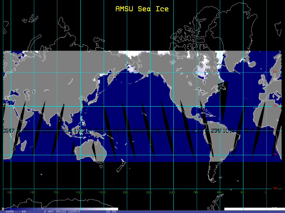
• Vertically integrated water vapor, liquid• Rain rate• Sea Ice• Ocean Surface Wind Speed• 85 GHz ice scattering signal useful for

tropical cyclone analysis– Highlights convectively active regions below

cirrus canopy seen in IR imagery

A: B: C:

A: Uses SSM/I Rain RatesB: AE uses GOES Longwave IR (Channel 4)C. GMSRA Combines all GOES channels

Ocean Surface Winds from SSM/I

• Passive Microwave (SSM/I, TMI)

– 19 GHz emissivity increases as capillary waves and sea foam are generated by wind

– Rain, thick clouds degrade algorithm

– Combine 19V GHz, 22V GHz, 37V GHz, 37H GHz

– Winds limited to ~40 kt– Provides speed but not

direction

Hurricane Jeanne 23 Sept 98

IR VIS

85 GHz Comp.

(From NRL web-site).

Properties of NOAA-15

• Polar orbiting satellite• 833 km above earth’s surface• 14.2 revolutions per day• Launched May 13, 1998 (Vandenberg

AFB)• Instrumentation:

– AVHRR, HIRS, AMSU, SBUV• First in new series (NOAA-K,L,M)• NOAA-16 Launched Fall 2000

AMSU Instrument Properties

• AMSU-A1– 13 frequencies 50-89 GHz– 48 km maximum resolution– Vertical temperature profiles 0-45 km

• AMSU-A2– 2 frequencies 23.8, 31.4 GHz– 48 km maximum resolution– Precipitable water, cloud water, rain rate

• AMSU-B (interference problems)– 5 frequencies: 89-183 GHz– 16 km maximum resolution– Water vapor soundings

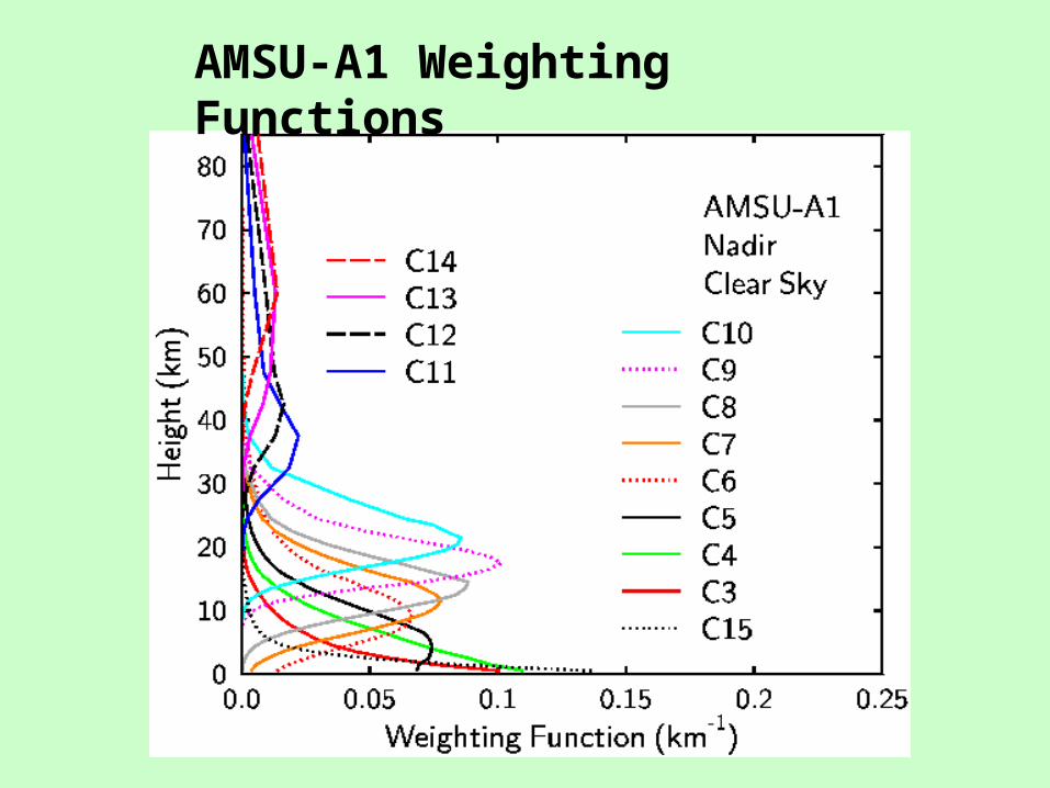
AMSU-A1 Weighting Functions

AMSU-A2 Weighting Functions

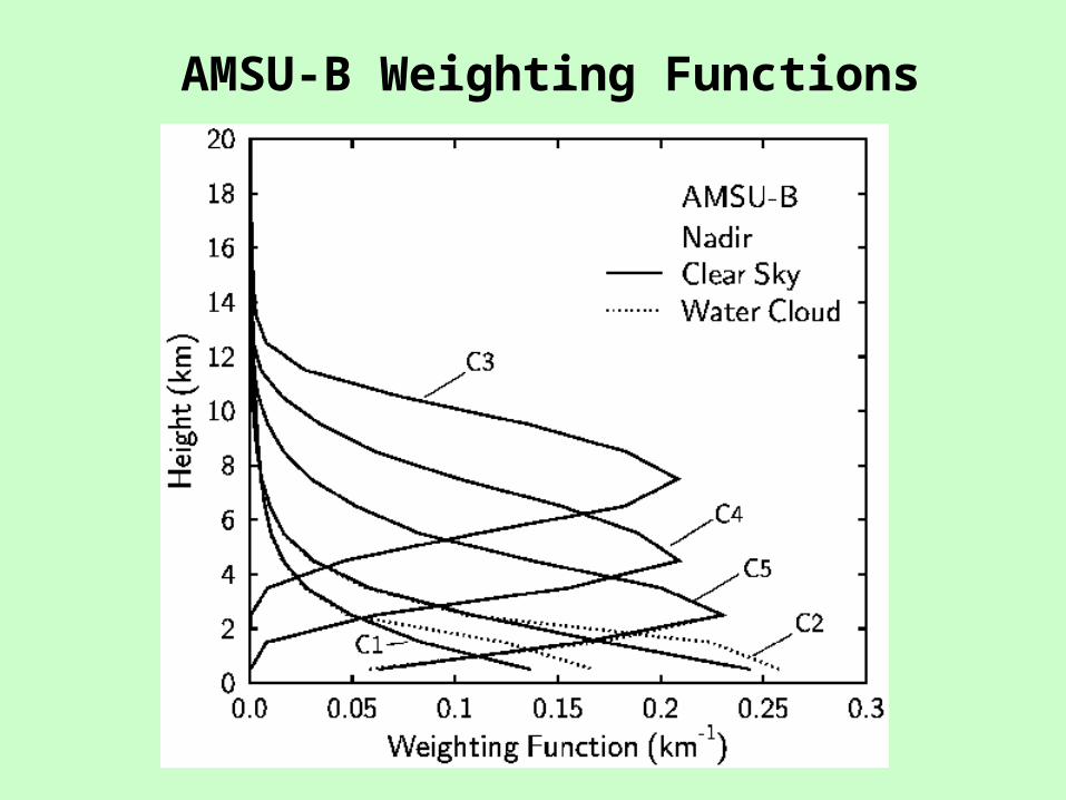
AMSU-B Weighting Functions

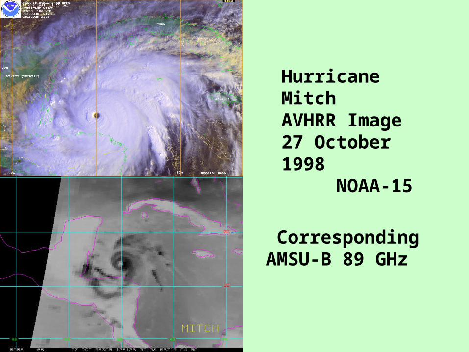
Hurricane MitchAVHRR Image27 October 1998 NOAA-15

CorrespondingAMSU-B 89 GHz

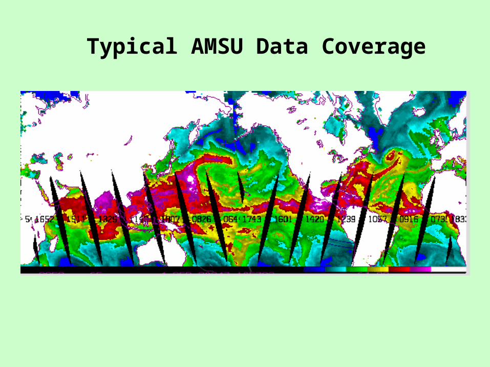
Typical AMSU Data Coverage

AMSU-A Moisture Algorithms• Total Precipitable Water (V)

– V = cos() * f[TB(23.8),TB(31.4)]

• Cloud Liquid Water (Q)– Q = cos( ) * g[TB(23.8),TB(31.4)]

• Rain Rate (R)– R = 0.002 * Q 1.7

• Tropical Rainfall Potential (TRaP)– TRaP = Ra * D/c

• Ra = avg. rain rate, D=storm dia., c = Storm Speed

AMSU-A Rainfall Rate for Hurricane Georges (.01 inches/hr) TRaP for Key West = 6.7 inches

Temperature Retrieval Algorithm

• 15 AMSU-A channels included• Radiances adjusted for side lobes before

conversion to brightness temperatures (BT)• BT adjusted for view angle• Statistical algorithm converts from BT to

temperature profiles• 40 vertical levels 0.1-1000 mb• RMS error 1.0-1.5 K compared with

rawindsondes

IR ImageryMarch 1, 1999

AMSU TemperatureRetrieval (570 mb)

AMSU Tropical Cyclone Applications

• Input for numerical models– Direct assimilation of AMSU radiances– Rain rate product input to physical initialization

procedures

• Apply hydrostatic/dynamical balance constraints to obtain height/wind fields – Height/winds input for intensity/structure

intensity estimation technique

Hydrostatic Balance

• Approximation to vertical momentum equation• Valid for horizontal scales > 10 km• dP/dz = -gP/RTv (Height coordinates)

– P=pressure, z=height, Tv=virtual temperature– G=gravitational constant, R=ideal gas constant– Allows calculation of pressure as a function of height P(z), given

temperature and moisture profile

• d /dp = -RTv/P (Pressure coordinates)– Allows calculatation of geopotential height as a function of

pressure (P)

• Both forms require boundary conditions – Integration can be upwards or downwards

• Contribution from moisture is fairly small and will be neglected (Tv replaced by T)

Dynamical Balance Conditions Provides Diagnostic Relationship Between Height and Wind

• High latitude, synoptic-scale flows– Geostrophic balance

• Axisymmetric flows– Gradient balance

• Higher-order approximation to the divergence equation– Charney balance equation

Geostrophic Balance(Not valid for tropical cyclones)

U/fL

Gradient Balance• Start with horizontal momentum equations in

cylindrical/pressure coordinates• Assume no variation in the azimuthal direction• Radial momentum equation reduces to:

V2/r + fV = d/dr

V = tangential wind, r = radius f = Coriolis parameter = geopotential height from hydrostatic equation

Charney Nonlinear Balance Equation

• NBE reduces to gradient wind in axisymmetric case• NBE reduces to geostrophic wind in low-amplitude

case

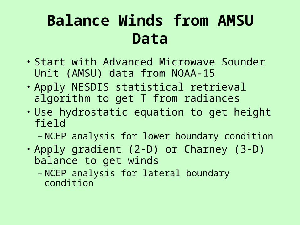
Balance Winds from AMSU Data

• Start with Advanced Microwave Sounder Unit (AMSU) data from NOAA-15

• Apply NESDIS statistical retrieval algorithm to get T from radiances

• Use hydrostatic equation to get height field– NCEP analysis for lower boundary condition

• Apply gradient (2-D) or Charney (3-D) balance to get winds– NCEP analysis for lateral boundary condition

2-D AMSU Wind Retrieval:Solution of the Gradient Wind Equation

• Gradient Wind Equation: V2/r + fV = r

– Find from V: = (V2/r + fV )dr

– Find V from : V = -fr/2 ± [(fr/2)2 + r r]1/2

• Requires choice of root and [(fr/2)2 + r r] > 0

2D Analyses - Hurricane Gert

Temperature(r,z) Sfc Pressure (x,y) Tangential Wind(r,z)U

ncor

rect

edH

ydro

met

eor

Cor

rect

ed

Correction for Attenuation by Cloud Liquid Water and Ice Scattering

• Use data base of 120 cases from 1999 hurricane season

• Derive statistical correction to temperature as a function of CLW for P < 300 hPa

• Identify isolated cold anomalies related to ice scattering using threshold technique

• “Patch” cold regions using Laplacian filter from surrounding data

2-D AMSU Wind Retrieval Results

• >250 cases analyzed in Atlantic and East Pacific basins during 1999-2000

• Inner core winds not resolved due to limited AMSU-A spatial resolution– Statistical relationship between AMSU analyses and

intensity

• Large differences in storm sizes– Useful for wind radii estimation

• Analyses appear to capture vertical structure changes• 2-D analysis algorithm available for evaluation in

West Pacific

AMSU 2-D WindsFor Large and Small Storms

Isaac 092800 120 kt Joyce 092700 70 kt

AMSU 2-D WindsIn Low-Shear andHigh-Shear StormEnvironments. (Note the deepercyclonic flow in thelow-shear cases.)

Low-Shear High-Shear

Statistical Intensity Estimation

• AMSU resolution prevents direct measurement of inner core

• Correlate parameters from AMSU analyses with observed storm intensity

• AMSU Predictors from 1999 storm sample:– r=600 to r=0 km pressure drop– Max tangential wind at 0 and 3 km– Max upper-level temperature anomaly– Average cloud-liquid water

• Algorithm explains 70% of variance• Algorithm will be tested on 2000 data

R2 = 0.72

0

20

40

60

80

100

120

140

0 20 40 60 80 100 120 140

Predicted Max Wind (kt)

Ob

se

rve

d M

ax

Win

d (

kt)

Predicted vs. Observerd Maximum Winds(Preliminary Results with Dependent Data)

Statistical Size Estimation

• Correlate parameters from AMSU analyses with observed storm size– Average radius of 34, 50 and 64 kt winds

• AMSU Predictors from 1999 storm sample:– R=600 to r=0 km pressure drop– Max tangential wind at 0 and 3 km– Storm latitude– Estimated maximum wind– Average cloud-liquid water

• Algorithm explains ~80% of variance• Algorithm will be tested on 2000 data

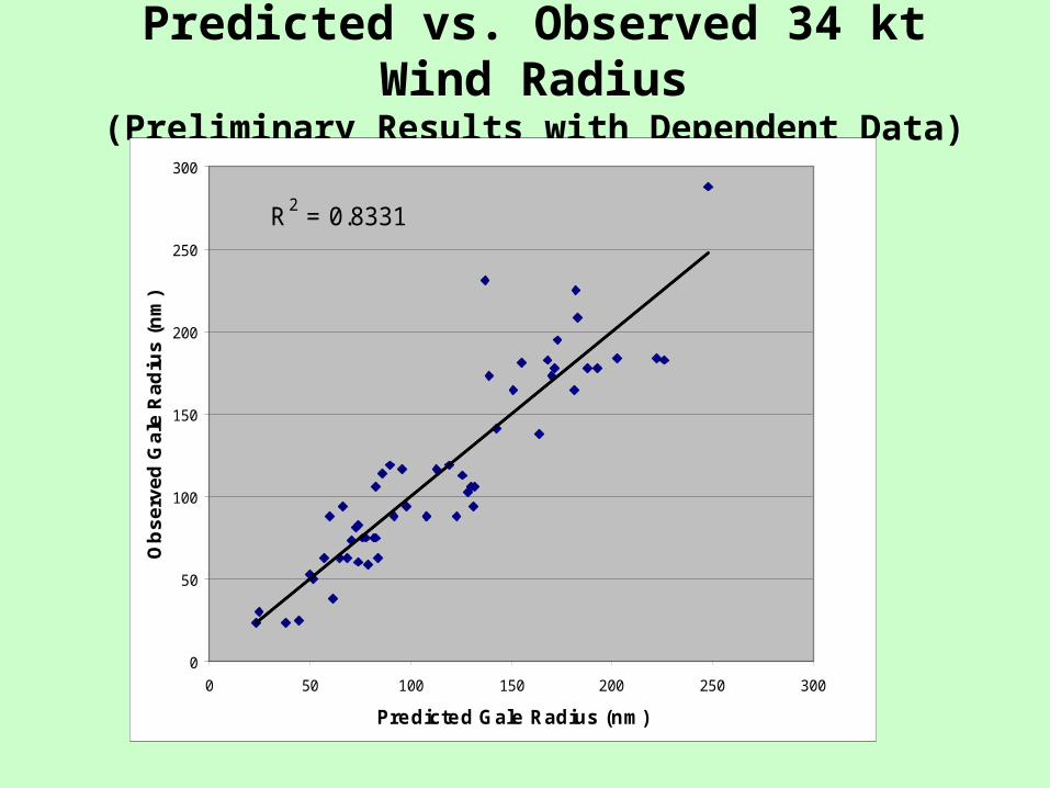
Predicted vs. Observed 34 kt Wind Radius(Preliminary Results with Dependent Data)

R2 = 0.8331

0

50

100

150

200

250

300

0 50 100 150 200 250 300

Predicted Gale Radius (nm)

Ob

se

rve

d G

ale

Ra

diu

s (

nm

)

3-D AMSU Wind Retrieval:Charney Nonlinear Balance Equation

• Charney balance equation:– 2 = -[(ux)2 +2vxuy + (vy)2] + f - u

• For nondivergent flow: u=-y, v= x, = 2– 2 = -2(xy)2 + 2(xx yy) + f 2 + y

• Find from u,v: Poisson equation– Requires boundary values for

• Find u,v from : Monge-Ampere Equation– Requires boundary values for u,v (or )

– Ellipticity condition: 2 + 1/2f2 > 0

– Possibility of two solutions

Charney Balance Equation Iterative Solution

• Developed for early NWP models

– Write balance equation as:

2 + f - [(ux)2 + (vx)2 + (uy)2 + (vy)2 + u+ 2 ] = 0

2 + f - [N ] = 0

where = 2 u = -y v= x

– Solve for :

= -(f/2) ± [(f/2)2 + N]1/2

– N = N() so iteration is necessary

Charney Balance Equation Variational Solution

• Iterative method sometimes fails for tropical cyclone case

• Variational solution method:– Define cost function as square of balance

equation integrated over domain of interest– Add smoothness penalty term to cost function– Find u,v to minimize cost function– Minimization requires cost function gradient,

determined from adjoint of balance equation– Boundary conditions for u,v from NCEP

analysis

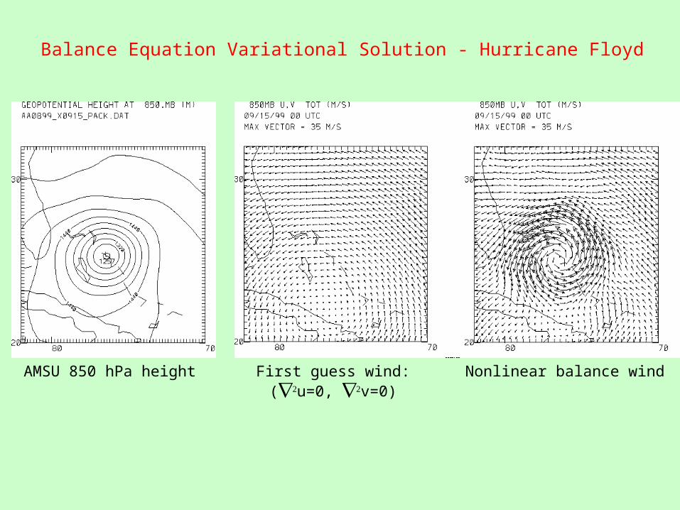
Balance Equation Variational Solution - Hurricane Floyd

AMSU 850 hPa height First guess wind:(u=0, v=0)

Nonlinear balance wind

Hurricane Floyd 850 mb Isotachs (kt) -80

-60

-40

-20

0

Evaluation of AMSU WindsRECON AMSU

Summary of Lesson 3

• Passive microwave data can penetrate through cloud tops

• Data available from DMSP(SSM/I), NOAA-15/16 (AMSU), and TRMM (TMI) satellites

• Algorithms available for ocean surface wind speed, integrated water content, rainfall rate, sea ice/snow cover

• Data useful for qualitative analysis of tropical cyclone structure (banding, eye wall, etc)

• AMSU temperature sounding can be combined with hydrostatic/dynamical balance constraints for tropical cyclone analysis