Triangle-intersecting Families of Graphs

David Ellis∗ Yuval Filmus †

Ehud Friedgut ‡

Dedicated to Vera T. Sos on occasion of her 80th birthday

September 2010

Abstract

A family of graphs F is triangle-intersecting if for every G, H ∈ F , G∩H contains a triangle.A conjecture of Simonovits and Sos from 1976 states that the largest triangle-intersecting familiesof graphs on a fixed set of n vertices are those obtained by fixing a specific triangle and takingall graphs containing it, resulting in a family of size 1

82(n2). We prove this conjecture and

some generalizations (for example, we prove that the same is true of odd-cycle-intersectingfamilies, and we obtain best possible bounds on the size of the family under different, notnecessarily uniform, measures). We also obtain stability results, showing that almost-largesttriangle-intersecting families have approximately the same structure.

1 Introduction

A basic theme in the field of extremal combinatorics is the study of the largest size of a structure(e.g. a family of sets) given some combinatorial information concerning it (e.g. restrictions onthe intersection of every two sets in the family.) The fundamental example of this is the Erdos-Ko-Rado theorem [6] which bounds the size of an intersecting family of k-element subsets of ann-element set (meaning a family in which any two sets have non-empty intersection). For k < n/2,the simple answer is that the unique largest intersecting families are those obtained by fixing anelement and choosing all k-sets containing it. This theorem is amenable to countless directionsof generalizations: demanding larger intersection size, having some arithmetic property of theintersection sizes, removing the restriction on the size of the sets while introducing some measureon the Boolean algebra of subsets of 1, . . . , n etc. etc. Usually, the aesthetically pleasing theoremsare those, like the EKR theorem, where the structure of the extremal families is simple to describe,often by focussing on a small set of elements through which membership in the family is determined.

A beautiful direction suggested by Simonovits and Sos is that of introducing structure on theground set, namely considering subgraphs of the complete graph on n vertices. They initiated theinvestigation in this direction with the following definition and question.

MSC 2010 subject classifications: 05C35,05D99Key words and phrases: Intersecting families, Graphs, Discrete Fourier analysis.

∗St John’s College, Cambridge, United Kingdom.†Department of Computer Science, University of Toronto. email: yuvalf@cs.toronto.edu. Supported by NSERC.‡Institute of Mathematics, Hebrew University, Jerusalem, Israel. email: ehud.friedgut@gmail.com Research sup-

ported in part by the Israel Science Foundation, grant no. 0397684.

1

Definition 1.1. A family of graphs F is triangle-intersecting if for every G, H ∈ F , G∩H containsa triangle.

Question 1 (Simonovits-Sos). What is the maximum size of a triangle-intersecting family of sub-graphs of the complete graph on n vertices?

They raised the natural conjecture that the largest families are precisely those given by fixinga triangle and taking all graphs containing this triangle. In this paper we prove their conjecture.

Theorem 1.2. Let F be a triangle-intersecting family of graphs on n vertices. Then |F| ≤ 182(n

2).Equality holds if and only if F consists of all graphs containing a fixed triangle.

Our main result in this paper is actually a strengthening of the above in several aspects. First,we relax the condition that the intersection of every two graphs in the family contains a triangle,and demand only that it contain an odd cycle (i.e. be non-bipartite). Secondly, we allow thesize of the family to be measured not only by the uniform measure on the set of all subgraphsof Kn, but rather according to the product measure of random graphs, G(n, p), for any p ≤ 1/2.Thirdly, for the case of the uniform measure, we relax the condition that for every two graphs Gand H in the family, G ∩ H contains a triangle, to the condition that G and H ‘agree’ on sometriangle — i.e. that there exists a triangle that is disjoint from the symmetric difference of G andH. Furthermore, we prove a stability result: any triangle-intersecting family that is sufficientlyclose in measure to the largest possible measure is actually close to a bona-fide extremal family.Finally, we observe that our proofs can be pushed further without much effort to prove a similarresult about (not necessarily uniform) hypergraphs — a result one might refer to as dealing withSchur-triple-intersecting families of binary vectors.

Before making all of the above precise and expanding a bit on our methods, let us introducesome necessary notation and definitions and review some relevant previous work.

1.1 Notation and main theorems

Let n be a positive integer, fixed throughout the paper. The power set of X will be denoted P(X).As usual, [n] denotes the set 1, 2, . . . , n. Also, [n](k) will denote S ⊆ [n] : |S| = k. It will be

convenient to think of the set of all subgraphs of Kn as the Abelian group Z[n](2)

2 where the groupoperation, which we denote by ⊕, is the symmetric difference (i.e. H ⊕G is the graph whose edgeset is the symmetric difference between the edge sets of G and H); we will also use the notation ∆for the same operator. We will write G for the complement of a graph G. Since we identify graphswith their edge sets, we will write |G| for the number of edges in G, and v(G) for the number ofnon-isolated vertices in G. We will denote the fact that G and H are isomorphic by G∼=H. If Gis the disjoint union of two graphs G1, G2 (that is, G1, G2 have no edges in common), then we willwrite G = G1 tG2.

Definition 1.3. A family F of subgraphs of Kn is triangle-intersecting (respectively odd-cycle-intersecting) if for every G, H ∈ F , G ∩ H contains a triangle (respectively an odd cycle). Wewill say that F is triangle-agreeing (respectively odd-cycle-agreeing) if for every G, H ∈ F , G⊕Hcontains a triangle (respectively an odd cycle).

Note that G∩H is contained in G⊕H, so a triangle-intersecting family is also triangle-agreeing.

2

Given F , a family of subgraphs of Kn, we will want to measure its size according to skew productmeasures: for any p ∈ [0, 1] and graph G on n vertices we will denote by µp(G) the probability thatG(n, p) = G, i.e.

µp(G) = p|G|(1− p)(n2)−|G|,

and for a family of graphs F we define µp(F) to be the probability that G(n, p) ∈ F , i.e.

µp(F) =∑G∈F

µp(G).

When p is fixed (e.g. throughout the section where p = 1/2) we will drop the subscript and simply

write µ(G) and µ(F). For any two functions f, g : Z[n](2)

2 → R we define their inner product as

〈f, g〉 = E(f · g) =∑G

µ(G)f(G)g(G).

We will denote the graph on n vertices with no edges by ∅. A k-forest is any forest with k edges.The graph on four vertices with 5 edges will be denoted by K−

4 . A biconnected component of agraph G means a maximal biconnected subgraph of G (i.e. it need not be an entire component).

If X is a finite set, P(X) will denote the power set of X, the set of all subsets of X. Identifyinga set with its characteristic function, we will often identify P(X) with 0, 1X = ZX

2 . A family Fof subsets of X is said to be an up-set if whenever S ∈ F and T ⊃ S, we have T ∈ F . The notation1P for a predicate P means 1 if P holds, and 0 if P doesn’t hold. If A is an Abelian group, andY ⊂ A, we write Γ(A, Y ) for the Cayley graph on A with generating set Y , meaning the graphwith vertex-set A and edge-set a, a + y : a ∈ A, y ∈ Y .

A Triangle junta is a family of all subgraphs of Kn with a prescribed intersection with a giventriangle. In the special case of the triangle junta being the family of all graphs containing a giventriangle, we will call this family a 4umvirate. (Don’t ask us how this is pronounced.)

Our main theorem is the following.

Theorem 1.4. • [Extremal families] Let p ≤ 1/2, and let F be an odd-cycle-intersectingfamily of subgraphs of Kn. Then µp(F) ≤ p3, with equality if and only if F is a 4umvirate.Furthermore, in the case p = 1/2, if F is odd-cycle-agreeing then µ(F) ≤ 1/8, with equalityif and only if F is a triangle junta.

• [Stability] For each p ≤ 1/2 there exists a constant cp (bounded for p ∈ [δ, 1/2], for any fixedδ > 0) such that for any ε ≥ 0, if F is an odd-cycle-intersecting family with µp(F) ≥ p3 − εthen there exists a 4umvirate T such that

µp(T ∆F) ≤ cpε.

For p = 1/2, the corresponding statement holds for odd-cycle-agreeing families.

The stability results, together with the fact that our theorem holds for all p ≤ 1/2, allow us todeduce a theorem concerning odd-cycle-intersecting families of graphs on n vertices with preciselyM edges, for M < 1

2

(n2

).

3

Corollary 1.5. Let α < 1/2 and let M = α(n2

). Let F be an odd-cycle-intersecting family of graphs

on n vertices with M edges each. Then

|F| ≤((

n2

)− 3

M − 3

).

Equality holds if and only if F is the set of all graphs with M edges containing a fixed triangle.Furthermore, if |F| > (1− ε)

((n2)−3

M−3

), then there exists a triangle T such that all but at most c · ε|F|

of the graphs in F contain T , where c = c(α).

This corollary follows in the footsteps of Corollary 1.7 in [8], and we omit its proof, since itis identical to the proof given there. It suffices to say that the idea of the proof is to study thefamily of all graphs containing a graph from F , and to apply Theorem 1.4 to it, together with someChernoff-type concentration of measure results.

We are also able to generalize our main theorem in the following manner, to not necessarilyuniform hypergraphs, although we will state the theorem in terms of characteristic vectors. Wediscovered this generalization while studying the question of families of subsets of Zn

2 such that theintersection of any two subsets contains a Schur triple, x, y, x + y.

Definition 1.6. We say that a family F of hypergraphs on [n] is odd-linear-dependency-intersectingif for any G, H ∈ F there exist l ∈ N and nonempty sets A1, A2, . . . , A2l+1 ∈ G ∩H such that

A14A24 . . .4A2l+1 = ∅.

Identifying subsets of [n] with their characteristic vectors in 0, 1n = Zn2 , we have the following

equivalent definition:

Definition 1.7. A family F of subsets of Zn2 is odd-linear-dependency-intersecting if for any two

subsets S, T ∈ F , there exist l ∈ N and non-zero vectors v1, v2, . . . , v2l+1 ∈ S ∩ T such that

v1 + v2 + . . . + v2l+1 = 0.

Naturally, an odd-linear-dependency-agreeing family is defined as above, with G∆H replacingG ∩H, and S∆T replacing S ∩ T .

Note that a Schur triple is a linearly dependent set of size 3, so a Schur-triple-intersecting familyis odd-linear-dependency-intersecting. We say that a family F of subsets of Zn

2 is a Schur-umvirateif there exists a Schur triple of non-zero vectors x, y, x + y such that F consists of all subsets ofZn

2 containing x, y, x+y. We say that F is a Schur junta if there exists a Schur triple x, y, x+ysuch that F consists of all subsets of Zn

2 with prescribed intersection with x, y, x + y.The definition of µp generalizes to families of subsets of Zn

2 in the obvious way. We have thefollowing:

Theorem 1.8. Let p ≤ 1/2, and let F be an odd-linear-dependency-intersecting family of subsetsof Zn

2 . Thenµp(F) ≤ p3.

Equality holds if and only if F is a Schur-umvirate. Moreover, for each p ≤ 1/2 there exists aconstant cp (bounded for p ∈ [δ, 1/2], for any fixed δ > 0) such that for any ε > 0, if µp(F) ≥ p3− εthen there exists a Schur-umvirate T such that

µp(T 4F) ≤ cpε.

For p = 1/2, the corresponding statements hold for odd-linear-dependency-agreeing families.

4

Remarks: Note that this is indeed a generalization, since any triangle-intersecting family ofgraphs can be lifted to a Schur-triple-intersecting family of hypergraphs by replacing every graphwith 22n−(n

2) hypergraphs in the obvious manner. In some ways, the proof of this version is simplerand more elegant. The fact that the ground set here is itself a vector space over Z2 highlights thefact that a triangle is not only a ‘triangle’, but in fact an ‘odd linear dependency over Z2’. Thismakes the use of discrete Fourier analysis, which by design captures parity issues, a natural choice.

Note that 0, 1n can be viewed as a vector matroid over Z2. Any odd linear dependency

v1 + v2 . . . + v2l+1 = 0

of non-zero vectors in 0, 1n contains a minimal odd linear dependency, i.e. an odd-sized circuitin the matroid. Hence, Theorem 1.8 can be seen as dealing with odd-circuit-intersecting familiesin a matroid over Z2.

We will defer the proof of Theorem 1.8 until section 5, and concentrate on the graph setting,which is easier to explain and to follow.

1.2 History

We referred above to the question of Simonovits and Sos as ‘beautiful’. For us this realizationcomes from studying their problem intensively, and realizing that the elementary combinatorialmethods (e.g. shifting) that are often applied to Erdos-Ko-Rado type problems do not work in thissetting, and that the structure on the ground set affects the nature of the question substantially.The main breakthroughs in this problem, the result of [4] that we expand below and the currentpaper, came from introducing more sophisticated machinery, which in retrospect seems to indicatethe tastefulness of the question.

There are two papers that we wish to mention in the prologue to our work, in order to sharpenour perspective. The main progress on the Simonovits-Sos conjecture since it was posed was madein [4], where it was proved that if F is a triangle-intersecting family, then µ(F) ≤ 1/4. This improvesupon the trivial bound of 1/2 (which follows from that fact that a graph and its complement cannotboth be in the family.) The method used in [4] is that of entropy/projections, and this is where thelemma known as Shearer’s entropy lemma is first stated. It is quite interesting that our methods,under a certain restriction, also give the bound of 1/4, although we do not see a direct connection(see Section 6.4). However, the trivial observation that is our starting point is common with [4]:given a triangle intersecting family F and a bipartite graph B, for any two graphs F1, F2 ∈ F itholds that F1∩F2 must have a non-empty intersection with B, as a triangle cannot be contained ina bipartite graph. The approach in [4] was to study the projections of F on various graphs B (thechoice they made was taking B to be a complete bipartite graph). We will also use this observationand study intersections with various choices of B, but from a slightly different angle.

Here are several remarks relevant to [4] that are quite useful in the current paper.

• The proof given in [4] used the fact that B is bipartite, not only triangle-free, hence it actuallyholds if triangle-intersecting is replaced by odd-cycle-intersecting. This will be true of ourproof too.

• In [4], it was observed that given a triangle-agreeing family, one can, by a series of monotoneshifts, transform it into a triangle-intersecting family of the same size (see section 2.3). Hence,

5

the maximum size of a triangle-agreeing family is equal to the maximum size of a triangle-intersecting family. In fact, the proof in [4] also goes through for odd-cycle-agreeing families.The same will be true of our proof, in the uniform measure case (p = 1/2).

• A different way of stating the basic observation is that if G ∈ F and B is a bipartite graphthen

G ∈ F ⇒ (G⊕B) 6∈ F . (1)

This immediately suggests working in the group setting, and replacing ‘intersecting’ with‘agreeing’.

• Although the uniform measure is perhaps the most natural one to study, the question makesperfect sense for any measure on the subgraphs of Kn, specifically for the probability measureµp induced by the random graph model G(n, p), defined above. The proof in [4] can bemodified to give the bound p2 for any p ≤ 1/2. We improve this to p3, and conjecture thatthis holds for any p ≤ 3/4 (see the open problems section at the end of this paper).

A second paper that is a thematic forerunner of the current one is [8]. It deals with thequestion of the largest measure of t-intersecting families, using spectral methods. The immediategeneralization of the EKR theorem, appearing already in [6], is the case of t-intersecting families.For any fixed integer t ≥ 2, we say that a family of subsets of [n] is t-intersecting if the intersectionof any two members of the family has size at least t. EKR showed that for any k, if n is sufficientlylarge depending on k, then the unique largest t-intersecting families of k-subsets of [n] are thoseobtained by taking all k-subsets containing t specific elements. Note that this is not necessarilytrue for smaller values of n, where a better construction can be, for example, all subsets containingat least t+1 elements from a fixed set of t+2 elements. In their paper [1], appropriately titled ‘Thecomplete intersection theorem for systems of finite sets’, Ahlswede and Khachatrian characterizedthe largest t-intersecting families for every value of n, k and t.

In [8], the question of t-intersecting families is studied in the setting of the product measure ofthe Boolean lattice P([n]). Let p ∈ (0, 1) be fixed. A p-random subset of [n] is a random subset of[n] produced by selecting each i ∈ [n] independently at random with probability p. We define theproduct measure µp on P([n]) as follows. For any set S ⊂ [n] define

µp(S) = p|S|(1− p)n−|S|,

i.e. the probability that a p-random subset of [n] is equal to S. For a family F of subsets of [n],we define

µp(F) =∑S∈F

µp(S).

It is well known that for p ≤ 1/2, the largest possible measure of an intersecting family is p, andfor p < 1/2, the unique largest-measure families consist of all sets containing a given element. Fort ≥ 1 it is shown in [8] that for p < 1

t+1 , the unique largest-measure t-intersecting families aret-umvirates, the families of sets defined by containing t fixed elements. Stability results are alsoproved. From this it follows immediately, for example, that Theorem 1.4 holds for all p ∈ (0, 1/4) ifthe constant c is allowed to depend on p. In the following subsection, we will discuss the relevanceof the methods of [8] to our paper.

6

1.3 Methods

The reason we mention [8] in our prologue is that we are following the path set there, of applyingan eigenvalue approach to an intersection problem (and skew Fourier analysis for the non-uniformmeasure). These spectral methods appear in similar settings in several much earlier papers (e.g.[11, 16], to mention a few), but here they are tailored to our needs in a manner that is inspiredby [8]. In what follows below, we introduce at a pedestrian pace the spectral engine that carriesthe proof.

Let us return to equation (1). If F is a triangle-intersecting family (or even an odd-cycle-agreeingfamily) and B is a bipartite graph then we have

G ∈ F ⇒ (G⊕B) 6∈ F .

So flipping the edges of B takes a graph in the family and produces a graph not in the family. Letus lift this operation to an operator AB acting on functions whose domain is the set of subgraphsof Kn, or equivalently, 0, 1[n](2) = Z[n](2)

2 . The definition is simple:

ABf(G) = f(G + B).

Of course, this works equally well if we choose B at random from some distribution B over bipartitegraphs, producing an operator which is an average of AB’s:

ABf(G) = E[f(G + B)],

where the expectation is over a random choice of B from B.The important property of AB for us is that if f is the characteristic function of F , then

whenever f(G) = 1, we have ABf(G) = 0, so f ·AB(f) ≡ 0, and in particular

〈f,ABf〉 = 0.

Now, of course, we can do this for any appropriate choice of B, and take (not necessarily positive) lin-ear combinations of several such operators, i.e. define an operator A of the type A(f) =

∑cBAB(f).

Clearly A too has the property that〈f,Af〉 = 0. (2)

The next step is to identify the eigenvalues and eigenfunctions of A and use equation (2) toextract information about the Fourier transform of f , and ultimately deduce information about F .This eigenvalue approach in such a context stems, most probably, from Hoffman’s bounds on thesize of an independent set in a regular graph, [11]. The extension we apply to deduce uniquenessand stability is essentially reproducing the exposition of [8] in our setting.

It turns out that when the distribution B is easy to understand then the spectral properties ofAB are also extremely easy to describe, and most fortunately, for every choice of B one has theprecise same set of eigenvectors (whose eigenvalues depend on B), making the linear combination∑

cBAB particularly easy to understand and analyze.Finally, in one sentence, we explain why fourteen years passed between the moment in which

Vera Sos asked the third author the question treated in this paper, and the resolution of theproblem: even after discovering the spectral path, how does one choose the distributions B and theappropriate weights cB in a way which produces the correct eigenvalues? Most of the paper dealswith the answer to that question.

7

1.4 Structure of the paper

We will treat the cases of p = 1/2 and p < 1/2 separately, since the latter is slightly more complexand less routine. In section 2 we begin the case of p = 1/2, and describe the main tools that wewill use for the proof. In section 2.4 we construct the operators and spectra that prove our maintheorem. In section 3 we study the cut statistics of random cuts of a graph, and prove the necessaryfacts that show that our operators have the desired properties. In section 4 we treat the case ofp < 1/2. In section 5 we prove the more general theorem on Schur-triple-intersecting families. Insection 6 we conclude with some related open problems.

2 The uniform measure, p = 1/2

2.1 Fourier Analysis

We briefly recall the essentials of Fourier Analysis on the Abelian group ZX2 , where X is a finite set.

(In our case, the set X will usually be [n](2), the edge-set of the complete graph Kn, and subsetsS ⊂ X will be replaced by subgraphs G ⊂ Kn.) We identify ZX

2 with the power-set of X in thenatural way, i.e. a subset of X corresponds to its characteristic function.

For any two functions f, g : ZX2 → R, we define their inner product as

〈f, g〉 = E(f · g) =1

2|X|

∑S⊂X

f(S)g(S);

this makes R[ZX2 ] into an inner-product space. For every subset R ⊂ X, we define a function

χR : ZX2 → R by

χR(S) = (−1)|R∩S|.

Then χR is a character of the group ZX2 , since for any S, T ⊂ X, we clearly have

χR(S ⊕ T ) = χR(S) · χR(T ).

It is routine to verify that the set χR : R ⊂ X is an orthonormal basis for the vector space R[ZX2 ]

of all real-valued functions on ZX2 ; it is called the Fourier-Walsh basis. Hence, every f : ZX

2 → Rhas a unique expansion of the form

f =∑R⊂X

f(R)χR; (3)

we have f(R) = 〈f, χR〉. We call (3) the Fourier expansion of f . From orthonormality, for any twofunctions f, g, we have Parseval’s Identity:

〈f, g〉 =∑R⊂X

f(R)g(R).

In particular, whenever f is Boolean (0/1 valued), taking g ≡ 1 gives:

f(∅) = 〈f,1〉 = E [f ] = E [f2] = 〈f, f〉 =∑R⊂X

f2(R).

8

Abusing notation, we will let F denote both a family of sets and its characteristic function, so theabove will be used in the form

µ(F) = F(∅) =∑R⊂X

F2(R).

Another formula that is useful to keep in the back of our minds is the convolution formula:

f ∗ g = f · g,

where f ∗ g(S) =∑

T⊂X f(T )g(S + T ).

2.2 Cayley operators and their spectra

Questions about largest intersecting families can often be translated into the question of findinga largest independent set in an appropriate graph (often a Cayley graph). One can then use thespectral approach due to Hoffman [11] to bound the size of the largest independent set in termsof the eigenvalues of the graph (meaning the eigenvalues of its adjacency matrix). A central ideain [5] and [8] is that one may choose appropriate weights on the edges of this graph to perturbthe operator defined by the adjacency matrix, and improve these bounds. These weights need notnecessarily be positive. In this paper, we will call these perturbed operators Odd-Cycle-Cayleyoperators, or OCC operators for short. The Cayley graph Γ that we have is on the group Z[n](2)

2 ,with the set of generators consisting of all graphs B such that B is a bipartite graph,

Γ = Γ(Z[n](2)

2 , B : B ⊂ Kn, B is bipartite)

.

Note that an odd-cycle-agreeing family of subgraphs of Kn is precisely an independent set in thisgraph.

Definition 2.1. A linear operator A on real-valued functions on Z[n](2)

2 will be called Odd-Cycle-Cayley, or OCC for short, if it has the following two properties:

1. If F is an odd-cycle-agreeing family, and f is its characteristic function, then

f(G) = 1 ⇒ Af(G) = 0.

2. The Fourier-Walsh basis is a (complete) set of eigenfunctions of A.

For each G ⊂ Kn, we write λG for the eigenvalue corresponding to the eigenfunction χG. Wewrite Λ = (λG)G⊂Kn for the vector of eigenvalues of the OCC operator; we call this an OCCspectrum. We denote the minimum eigenvalue by λmin, and we write Λmin for the set of graphs Gwith λG = λmin; we will call these the ‘tight graphs’. The spectral gap of Λ is the maximal γ suchthat λH ≥ λmin + γ for all H 6∈ Λmin.

Note that the set of OCC operators forms a linear space, and hence also the set of OCC spectrais a linear space, a fact that is of crucial importance for us.

Our main tool for constructing OCC operators is by using Equation 1 as described in subsection1.3 where we discussed our methods. Let B be a bipartite graph, and let AB be the operator onreal-valued functions on Z[n](2)

2 , defined by

ABf(G) = f(G + B).

9

Similarly, let B be a distribution over bipartite graphs, and let

ABf(G) = E[f(G⊕B)],

where the expectation is over a choice of B from B. We make the following

Claim 1. AB is an OCC operator, and its spectrum is given by

λR = (−1)|R| E[χB(R)].

Before proving the claim, we list several equivalent ways of describing AB, depending on one’smathematical taste:

• AB is a convolution operator, and therefore has the elements of the Fourier-Walsh basis aseigenfunctions.

• AB is the average of operators AB. Note that AB is a tensor product of(n2

)operators (one for

each edge of Kn), each acting on functions on a two-point space. Hence, the eigenfunctionsof each AB include the tensor products of the eigenfunctions from each coordinate, which,again, is the Fourier-Walsh basis. Therefore, the same is true of AB.

• Alternatively, note that AB is the operator defined by the adjacency matrix of the Cayleygraph on Z[n](2)

2 with generating set B, which is a subgraph of Γ. It is well-known thatthe eigenvectors of the adjacency matrix of any Cayley graph on an Abelian group includethe characters of the group, i.e. the Fourier-Walsh basis in our case.

• AB is a Markov operator describing a random walk on Z[n](2)

2 . This random walk has theuniform measure as its stationary measure and has the property that if F is odd-cycle-intersecting then two consecutive steps cannot both lie in F .

This last characterization, which may seem less appealing, will become quite illuminating once wemove to the setting of µp for p < 1/2.

Proof of Claim 1: It is clear that if F is an odd-cycle-agreeing family, and f its characteristicfunction then

f(G) = 1 ⇒ ABf(G) = 0.

It is also quite simple to verify that the Fourier-Walsh characters are eigenfunctions of AB, and togive an explicit formula for the eigenvalues:

ABχR(G) = E[χR(G⊕B)] = χR(G) · E[χR(B)],

henceλR = E[χR(B)].

It turns out to be slightly more useful to write this last expression as given by our claim:

λR = (−1)|R| E[χB(R)] = (−1)|R| E[χB(R ∩B)]. (4)

10

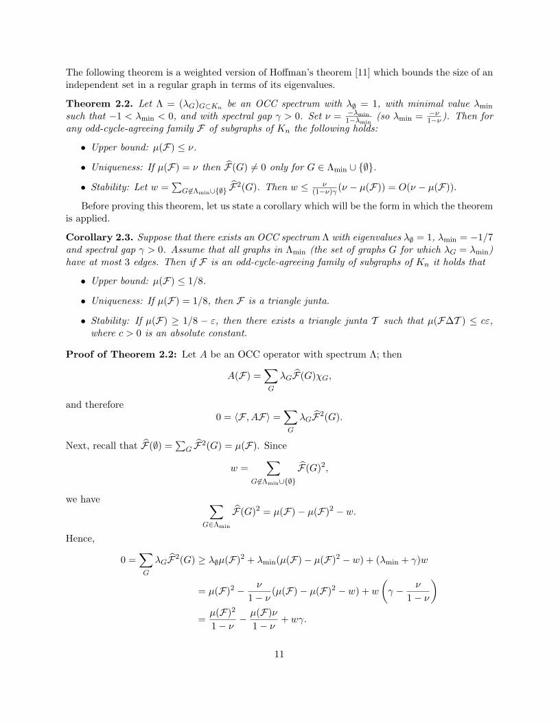
The following theorem is a weighted version of Hoffman’s theorem [11] which bounds the size of anindependent set in a regular graph in terms of its eigenvalues.

Theorem 2.2. Let Λ = (λG)G⊂Kn be an OCC spectrum with λ∅ = 1, with minimal value λmin

such that −1 < λmin < 0, and with spectral gap γ > 0. Set ν = −λmin1−λmin

(so λmin = −ν1−ν ). Then for

any odd-cycle-agreeing family F of subgraphs of Kn the following holds:

• Upper bound: µ(F) ≤ ν.

• Uniqueness: If µ(F) = ν then F(G) 6= 0 only for G ∈ Λmin ∪ ∅.

• Stability: Let w =∑

G6∈Λmin∪∅ F2(G). Then w ≤ ν

(1−ν)γ (ν − µ(F)) = O(ν − µ(F)).

Before proving this theorem, let us state a corollary which will be the form in which the theoremis applied.

Corollary 2.3. Suppose that there exists an OCC spectrum Λ with eigenvalues λ∅ = 1, λmin = −1/7and spectral gap γ > 0. Assume that all graphs in Λmin (the set of graphs G for which λG = λmin)have at most 3 edges. Then if F is an odd-cycle-agreeing family of subgraphs of Kn it holds that

• Upper bound: µ(F) ≤ 1/8.

• Uniqueness: If µ(F) = 1/8, then F is a triangle junta.

• Stability: If µ(F) ≥ 1/8 − ε, then there exists a triangle junta T such that µ(F∆T ) ≤ cε,where c > 0 is an absolute constant.

Proof of Theorem 2.2: Let A be an OCC operator with spectrum Λ; then

A(F) =∑G

λGF(G)χG,

and therefore0 = 〈F , AF〉 =

∑G

λGF2(G).

Next, recall that F(∅) =∑

G F2(G) = µ(F). Since

w =∑

G6∈Λmin∪∅

F(G)2,

we have ∑G∈Λmin

F(G)2 = µ(F)− µ(F)2 − w.

Hence,

0 =∑G

λGF2(G) ≥ λ∅µ(F)2 + λmin(µ(F)− µ(F)2 − w) + (λmin + γ)w

= µ(F)2 − ν

1− ν(µ(F)− µ(F)2 − w) + w

(γ − ν

1− ν

)=

µ(F)2

1− ν− µ(F)ν

1− ν+ wγ.

11

Therefore,µ(F)2 − µ(F)ν + wγ(1− ν) ≥ 0.

Since γ > 0, we immediately obtain µ(F) ≤ ν, with equality if and only if w = 0. Thus,

µ(F)2 − µ(F)ν + wγ(1− ν)µ(F)

ν≥ 0.

Cancelling and rearranging, we obtain:

w ≤ ν

(1− ν)γ(ν − µ(F)),

as required.

Proof of Corollary 2.3: The upper bound of 1/8 follows immediately from Theorem 2.2. Theuniqueness claim is a special case of [8, Lemma 2.8(1)], which we will quote below. The stabilityfollows from a powerful result of Kindler and Safra [13] (as was the case in [8].) We recall theirresult too.

• Uniqueness. We first prove the uniqueness under the assumption that F is odd-cycle-intersecting. The reduction from the agreeing case to the intersecting case is done in Lemma 2.7in the following subsection.

Since we know that the Fourier transform of F is concentrated on graphs with at most 3 edges,it follows from a result of Nisan and Szegedy [14, Theorem 2.1] that F depends on at most 3·23 = 24coordinates, i.e. can be described by the intersection of its members with a graph on 24 edges.However, even with a computer it seems extremely difficult to check all such examples. Luckilyfor us we have two additional assumptions. First, we may assume that F is an up-set, else we canreplace it by its up-filter, the family of all graphs containing a member of F , which would preservethe intersection property. Secondly, we have µ(F) = 1/8. This falls precisely into the setting ofthe following lemma.

Lemma 2.4 ( [8] ). Let N ∈ N, let p ≤ 1/2 and suppose f : 0, 1N → 0, 1 is a monotoneBoolean function with Ep f = pt, and f(S) = 0 whenever |S| > t. Then f is a t-umvirate (dependsonly on t coordinates).

(Here, the expectation Ep is taken with respect to the skew product measure µp on 0, 1N ;in our case, p = 1/2.) Clearly, in our case, if F is triangle-intersecting and a 3-umvirate, it is a4umvirate. The reduction from odd-cycle-agreeing families to odd-cycle-intersecting families is inLemma 2.7

• Stability. We need Theorem 3 from [13]:

Theorem 2.5 (Kindler-Safra). For every t ∈ N, there exist ε0 > 0, c0 > 0 and T0 ∈ N such thatthe following holds. Let N ∈ N, and let f : 0, 1N → 0, 1 be a Boolean function such that∑

|S|>t

f(S)2 = ε < ε0.

Then there exists a Boolean function g : 0, 1N → 0, 1, depending on at most T0 coordinates,such that

µ(R : f(R) 6= g(R)) ≤ c0ε.

12

The nice thing about this theorem is that as soon as the Fourier weight on the higher levels issmall enough, the number of coordinates needed for the approximating family does not grow. Weapply this in our setting as follows. Assume that F is an odd-cycle-agreeing family of subgraphsof Kn with µ(F) > 1/8− ε. From Theorem 2.2, we have

w =∑

G6∈Λmin∪∅

F(G)2 ≤ 17γ

ε.

Applying the Kindler-Safra result with t = 3, we see that provided ε ≤ 7γε0, F is ( c07γ ε)-close to

some family depending on at most T coordinates (edges). But there are only a finite number of suchfamilies that are not triangle juntas, and by our uniqueness result, all have measure less than 1/8.Choose ε1 > 0 such that all of these families have measure less than 1/8− (1 + c0

7γ )ε1. If ε ≤ ε1, Fcannot have measure at least 1/8−ε and be ( c0

7γ ε)-close to one of these families, so the approximatingfamily guaranteed by Kindler-Safra must be a triangle junta. If ε > min(7γε0, ε1) =: ε2, we maysimply choose the constant c = 1/ε2, completing the proof of Corollary 2.3.

2.3 The intersecting / agreeing equivalence

In the proof of the uniqueness statement in Corollary 2.3 we assumed that the family of graphs inquestion was odd-cycle-intersecting. We now wish to reduce the general case of odd-cycle-agreeingto that of odd-cycle-intersecting. To this end, it will be helpful to return to the related observationof Chung, Frankl, Graham and Shearer in [4] mentioned earlier. For completeness, we reproducetheir general statement and proof, as we will wish to build upon it.

Let X be a finite set, and let Z ⊂ P(X) be a family of subsets of X. We say that a familyF ⊂ P(X) is Z-intersecting if for any A,B ∈ F there exists Z ∈ Z such that Z ⊂ A ∩B. We saythat F ⊂ P(X) is Z-agreeing if for any A,B ∈ F there exists Z ∈ Z such that Z ∩ (A∆B) = ∅.We write

m(Z) = max|A| : A ⊂ PX, A is Z-intersecting

andm(Z) = max|A| : A ⊂ PX, A is Z-agreeing.

Chung, Frankl, Graham and Shearer proved the following:

Lemma 2.6. Let X be a finite set, and let Z ⊂ P(X). Then m(Z) = m(Z).

Proof : Clearly, a Z-intersecting family is Z-agreeing, and therefore m(Z) ≤ m(Z). We will showthat any Z-agreeing family can be made into a Z-intersecting family of the same size.

For any i ∈ X, consider the i-monotonization operation Ci, defined as follows. Given a familyA ⊂ P(X), Ci(A) is produced by replacing A with A ∪ i for each set A such that i /∈ A, A ∈ Aand A ∪ i /∈ A. (Note that Ci is a special case of the so-called UV -compression CUV , withU = i and V = ∅. The reader may refer to [7] for a discussion of UV -compressions and theiruses in combinatorics.)

Clearly, |Ci(A)| = |A|; it is easy to check that if A is Z-agreeing then so is Ci(A).Now let F ⊂ P(X) be a Z-agreeing family, and successively apply the operations Ci for i ∈ X.

Formally, we set F0 = F ; given Fk, if there exists F ∈ Fk and i ∈ X such that F ∪ i /∈ Fk,then we let Fk+1 = Ci(Fk). At each stage of the process, the sum of the sizes of the sets in thefamily increases by at least 1, so the process must terminate, say with the family Fl. Let F ′ = Fl.

13

Observe that F ′ is a Z-agreeing family with |F ′| = |F|. Moreover, it is an up-set, meaning that ifF ∈ F ′ and G ⊃ F , then G ∈ F ′. It follows that F ′ must be Z-intersecting. (If F,G ∈ F ′, thenF ∪G ∈ F ′, so there exists Z ∈ Z such that ((F ∪G)∆G) ∩ Z = ∅. But then F ∩G ⊃ Z. Hence,F ′ is Z-intersecting.)

It follows that m(Z) ≤ m(Z), and therefore m(Z) = m(Z), as required.

We can now complete the proof of the uniqueness statement in Corollary 2.3, which claims thatif F is an odd-cycle-agreeing family and µ(F) = 1/8, then F is a triangle junta. We will apply themonotonization operations above to F , and produce an odd-cycle-intersecting family of the samesize, which by our results must be a 4umvirate. The following lemma then shows that F must bea triangle junta.

Lemma 2.7. Let F be an odd-cycle-agreeing family, and assume that a series of monotonizationoperations Ce (for e ∈ [n](2)) as described above produces a family Fk which is a 4umvirate. ThenF is a triangle junta.

Proof : Suppose Fk ⊂ Z[n](2)

2 is odd-cycle-agreeing, and Fk+1 = Ce(Fk) 6= Fk is a T -junta forsome triangle T ⊂ Kn. Then there exists a graph G /∈ Fk+1 such that G ∪ e ∈ Fk+1; since Fk+1

is a T -junta, we must have e ∈ T . Let S be the subgraph of T such that

Fk+1 = G ∈ Z[n](2)

2 : G ∩ T = S.

Clearly, e ∈ S. Let C = G ∈ Fk : e /∈ G, and let D = G ∈ Fk : e ∈ G; then we may express

Fk = C t D.

Observe that if G ∈ C, then G ∪ e /∈ D: if G ∈ C and G ∪ e ∈ D, then G, G ∪ e ∈ Fk+1,contradicting the fact that all graphs in Fk+1 contain S. Hence,

Fk+1 = D t G ∪ e : G ∈ C.

It follows that all graphs G ∈ D have G ∩ T = S, and all graphs G ∈ C have G ∩ T = S − e. SinceFk+1 6= Fk, we must have C 6= ∅; we will show that D = ∅. Suppose for a contradiction that D 6= ∅.Let |D| = N ≥ 1; then |C| = 2(n

2)−3 −N ≥ 1. Since T ⊕ e intersects every triangle, if G ∈ Fk thenG⊕ (T ⊕ e) /∈ Fk. Since

|C|+ |D| = 2(n2)−3,

for every H ⊂ T exactly one of H⊕S ∈ D and H⊕S⊕T ⊕e ∈ C holds. In other words, the classes

V = H ⊂ T : H ⊕ S ∈ D, W = H ⊂ T : H ⊕ S ⊕ T ⊕ e ∈ C

form a partition of the set of labeled subgraphs of T , with both classes nonempty. Hence, thereexist two adjacent subgraphs of T in different classes, i.e. there exists a subgraph H ⊂ T and anedge f ∈ E(T ) such that H ⊕ S ∈ D, and H ⊕ f ⊕ S ⊕ T ⊕ e ∈ C. But these two graphs agree onlyon the graph T ⊕ e⊕ f , which is a 3-edge graph containing exactly two edges of the triangle T , socannot be a triangle. This contradicts our assumption that Fk is odd-cycle-agreeing.

We may conclude that D = ∅, i.e.

Fk = G ∈ Gn : G ∩ T = S − e.

Hence, Fk is also a T -junta.By backwards induction on k, we see that F0 = F is also a T -junta, completing the proof.

14

2.4 Constructing the required OCC spectrum

In this section we prove the existence of an OCC operator with the desired spectrum, which togetherwith Corollary 2.3 will complete the proof of Theorem 1.4 for the case of p = 1/2. Our constructionwill proceed in two steps. First, we prove the existence of an OCC spectrum Λ(1) with the correctminimal eigenvalue, but for which Λmin, the set of graphs on which it is obtained, includes also4-forests and K−

4 . We then take care of these extra graphs by adding a multiple of Λ(2), an OCCspectrum that takes positive value on these problematic graphs while having value 0 for all graphswith three or less edges.

The main lemma we use is extremely easy to state and prove, yet turns out to be very useful.

Lemma 2.8. Let B be a distribution on bipartite graphs, and for every B ∈ B let fB be a real-valued function whose domain is the set of subgraphs of B. Then the following function is an OCCspectrum:

λG = (−1)|G| E[fB(B ∩G)],

where, as usual, the expectation is with respect to a random choice of B from B.

Proof : Fix a bipartite graph B. From Claim 1, we know that AB is an OCC operator. Equiv-alently, from equation (4), λG = (−1)|G|χB(G ∩ B) is an OCC spectrum. Moreover, if B′ is anysubgraph of B, the function (−1)|G|χB′(G∩B) = (−1)|G|χB′(G∩B′) also describes an OCC spec-trum. Since the set χB′ : B′ ⊂ B spans all functions f on the subgraphs of B, we see that forany choice of f , the vector described by λG = (−1)|G|f(G ∩ B) is also an OCC spectrum. Takingexpectation with respect to a random choice of B from B completes the proof.

The few choices of fB and B for which we will apply this lemma are quite simple. The distribution Bwill always be the uniform distribution on complete bipartite subgraphs of Kn, and the functions fB

will always be invariant under isomorphism of subgraphs of B. Hence, our OCC spectra (λG)G⊂Kn

will always be invariant under graph isomorphism, so they may be seen as functions on the set ofunlabelled graphs with at most n vertices. In fact, we will choose fB(G ∩ B) to be the indicatorfunction of the event that the number of edges of G∩B is i (for i = 1, 2 or 3), or to be the indicatorfunction of G ∩B being isomorphic to a given graph R (for some small list of R’s).

Corollary 2.9. Let (V1, V2) be a random bipartition of the vertices of Kn, where each vertex ischosen independently to belong to each Vi with probability 1/2. Let B be the set of edges of Kn

between V1 and V2. For any graph G ⊆ Kn, let

qi(G) = Pr[|G ∩B| = i],

and for any bipartite graph R, let

qR(G) = Pr[(G ∩B)∼=R],

where H ∼=R means that H is isomorphic to R; all probabilities are over the choice of the randombipartition. Then for any integer i,

λG = (−1)|G|qi(G)

is an OCC spectrum, and for any bipartite graph R,

(−1)|G|qR(G)

is an OCC spectrum.

15

Recall that if G is a graph, a cut in G is a bipartite subgraph of G produced by partitioningthe vertices of G into two classes V1 and V2, and taking all the edges of G that go between thetwo classes. If V1, V2 and B are as above, G ∩B is called a (uniform) random cut in G. Note thatqi(G) is the probability that a random cut in G has exactly i edges, so is relatively easy to analyze;qR(G) is the probability that a random cut in G is isomorphic to R.

The beauty of the functions qi(G) and qR(G) is that they supply us with a rich enough spaceof eigenvalues to create a spectrum with the correct values on small graphs, yet they decay quicklywith the size of G, ensuring that the eigenvalues of larger graphs will be bounded away from λmin.When tackling the problem, we tried taking a linear combination of as few as possible of thesebuilding blocks, constructing an OCC spectrum that obtains the desired values on subgraphs ofthe triangle; we prayed that this is feasible, and that the resulting eigenvalues for larger graphsmaintain a spectral gap. Happily, with some fine tuning, this works. This is manifested in thefollowing two claims.

Claim 2. Let Λ(1) be the OCC spectrum described by

λ(1)G = (−1)|G|

[q0(G)− 5

7q1(G)− 1

7q2(G) +

328

q3(G)]

.

Then

• λ(1)∅ = 1.

• λ(1)min = −1/7.

• Λ(1)min consists of the following graphs: a single edge, a path of length two, two disjoint edges,

a triangle, all forests with four edges, and K−4 .

• For all H 6∈ Λ(1)min it holds that λ

(1)H ≥ −1/7 + γ′, with γ′ = 1/56.

Claim 3. Let Λ(2) be the OCC spectrum described by

λ(2)G = (−1)|G|

[∑qF (G)− q(G)

]where the sum is over all 4-forests F , and denotes C4. Then

1. λ(2)H = 0 for all H with less than 4 edges.

2. λ(2)F = 1/16 for all 4-forests.

3. λ(2)

K−4

= 1/8.

4. |λ(2)G | ≤ 1 for all G.

We defer the proof of Claim 2 to the next section where we analyze the cut statistics of arandom cut of a graph. The proof of Claim 3 is quite easy.

Proof : We follow the items of the claim:

1. Clear: a cut in a graph with at most 3 edges has size at most 3.

16

2. For any forest, each edge belongs to a random cut independently of any other edge. Hence,qF (F ) = 2−|F | for any forest F . (See section 3 for more details). Also, q(F ) = 0 andqF (F ′) = 0 for any two distinct 4-forests F ,F ′.

3. Let the vertices of K−4 be labelled by a, b, c, d, where a and c are the vertices of degree 3.

Then a random cut in K−4 is isomorphic to C4 if and only if a and c belong to one side of the

cut, and b and d to the other side. This happens with probability 1/8 . Clearly, qF (K−4 ) = 0

for any 4-forest F : K−4 contains no 4-forest.

4. Finally, |λ(2)(G)| is the difference between two probabilities, hence is at most 1.

Taking a linear combination of the two OCC spectra from the previous claims gives us the desiredOCC spectrum, which completes the proof of our main theorem, Theorem 1.4, when p = 1/2.

Corollary 2.10. Let Λ = Λ(1) + 1617γ′Λ(2). Then Λ is an OCC spectrum as described in Corollary

2.3:

• λ∅ = 1.

• λG = −1/7 for all non-empty subgraphs G of K3 (and for the graph consisting of two disjointedges).

• Letting γ = 117γ′ gives that λG ≥ −1/7 + γ for any G with more than three edges.

Proof : Note that for any 4-forest F , the new eigenvalue λF is now equal to −1/7 + 1617

116γ′, the

eigenvalue λK−4

has increased to −1/7 + 1617

18γ′, and for all other non-empty graphs G we have

λG ≥ −1/7 + γ′ − 1617γ′.

3 Cut Statistics

The purpose of this section is to study the cut statistics of graphs for a (uniform) random cut,in order to prove Claim 2. We begin by using block-decompositions of graphs to simplify ourcalculations.

We will sometimes think of a random cut in G as being produced by a random red/blue colouringof V (G), where each vertex is independently coloured red or blue with probability 1/2. For ared/blue colouring c : V (G) → red,blue, we let Y (c) denote the number of edges in the associatedcut, i.e. the number of multicoloured edges.

Let Q(G) = (qk)k≥0 denote the distribution of |G ∩ B|; we call this the cut distribution of G.Let

QG(X) =∑k≥0

qk(G)Xk

denote the probability-generating function of |G ∩ B|. For example, if G is a single edge thenq0(−) = q1(−) = 1/2, and therefore

Q−(X) = 12 + 1

2X.

17

We will see that |G ∩ B| is a sum of independent random variables |H ∩ B|, where H ranges overcertain subgraphs of G. Probability-generating functions will be a convenient tool for us, since ifY1 and Y2 are independent random variables, we have QY1+Y2(X) = QY1(X)QY2(X).

In the rest of the section, we will study the cut distribution in enough detail so that we canprove Claim 2. But first, let us digress and explain how to construct Λ(1). We begin by consideringsome small graphs and their cut distributions:

G q0(G) q1(G) q2(G) q3(G) q4(G)∅ 1 0 0 0 0− 1/2 1/2 0 0 0∧ 1/4 1/2 1/4 0 04 1/4 0 3/4 0 0F4 1/16 4/16 6/16 4/16 1/16K−

4 1/8 0 1/4 1/2 1/8

In the table, F4 is a forest with 4 edges (they all have the same cut distribution).Suppose we are looking for an OCC spectrum of the form

λ(G) = (−1)|G| [c0q0(G) + c1q1(G) + c2q2(G) + c3q3(G) + c4q4(G)] .

Since λ(∅) = 1, c0 = 1. Applying the proof of Theorem 2.2 to a 4umvirate, whose Fouriertransform is concentrated on subgraphs of a triangle, shows that we need λ(G) = λmin = −1/7for all subgraphs of the triangle. This forces the choices c1 = −5/7 and c2 = −1/7. Substitutingc0, c1, c2 into the equations defined by F4 and K−

4 gives us a lower and upper bound (respectively)on 4c3 + c4. Both bounds coincide (what luck! This good fortune does not hold for p > 1/2),implying that 4c3 + c4 = 3/7. To simplify matters, we choose c4 = 0 and so c3 = 3/28.

The OCC spectrum of Λ(1) is engineered to work for the graphs appearing in the table. In therest of this section, we show that it also works for all other graphs.

Observe that if G = G1 tG2 then

QG(X) = QG1(X)QG2(X),

since G1 ∩B and G2 ∩B are independent, and |G ∩B| = |G1 ∩B|+ |G2 ∩B|.Let G be a connected graph, and suppose that v is a cutvertex of G, meaning a vertex whose

removal disconnects G. Suppose the removal of v separates G into components G[S1], . . . , G[SN ].For each i, let

Hi = G[Si ∪ v].

Observe that the system of random variables Hi ∩ B : i ∈ [N ] is independent, since for anyvertex v, the distribution of H ∩ B remains unchanged even if we fix the class of the vertex v, inwhich case the independence is immediate. Clearly,

|G ∩B| =N∑

i=1

|Hi ∩B|.

It follows that

QG(X) =N∏

i=1

QHi(X).

18

Let H =⊔

i Hi; H is produced by splitting the graph G at the vertex v. (For example, splittingthe graph ./ at the cutvertex in its centre produces the graph B C.) Then

QG(X) = QH(X).

Recall that a bridge of a graph G is an edge whose removal increases the number of connectedcomponents of G; a block of G is a bridge or a biconnected component of G. Note that if G isbridgeless then q1(G) = 0, since a cut of size 1 would be a bridge.

Observe that if G and G′ have the same number of bridges and the same number of blocksisomorphic to K for each biconnected graph K, then G and G′ have the same cut-distribution.In fact, if G has m bridges and tK blocks isomorphic to K (for each biconnected graph K), thenrepeating the above splitting process within every component until there are no more cutvertices,we end up producing a graph Gs which is a vertex-disjoint union of all the blocks of G. We call Gs

the split of G. We have:

QG(X) = QGs(X) = (12 + 1

2X)m∏

K∈K(QK(X))tK = 1

2m (1 + X)m∏

K∈K(QK(X))tK ,

where K denotes a set of representatives for the isomorphism classes of biconnected graphs. Forexample,

QB−C = (12 + 1

2X)(QC(X))2 = (12 + 1

2X)(14 + 3

4X2)2.

Now suppose G has exactly m bridges. Let H be the union of the biconnected components ofGs; write

QH(X) =∑i≥0

aiXi.

Here (ai)i≥0 is the cut distribution of H, so obviously,∑

i≥0 ai = 1. Note that a1 = 0, since H isbridgeless. We have

QG(X) = (12 + 1

2X)mQH(X)= 1

2m (1 + X)m(a0 + a2X2 + a3X

3 + . . .)= 1

2m

(1 + mX +

(m2

)X2 +

(m3

)X3 + . . .

) (a0 + a2X

2 + a3X3 + . . .

)= 1

2m

(a0 + ma0X +

((m2

)a0 + a2

)X2 +

((m3

)a0 + ma2 + a3

)X3 + R(X)X4

), (5)

where R(X) ∈ Q[X].

3.1 Proof of Claim 2

We will need the following additional facts about the cut distributions of graphs:

Lemma 3.1. Let G be a graph.

1. If G has exactly N connected components, then q0(G) = 2N−v(G).

2. If G has exactly m bridges, then q1(G) = mq0(G).

3. If G has a vertex with odd degree, then qk(G) ≤ 1/2 for any k ≥ 0.

4. For any odd k, qk(G) ≤ 1/2.

19

5. Always q2(G) ≤ 3/4.

Proof : We follow the items of the lemma:

1. If G has N connected components then G ∩ B = 0 iff all the vertices of each connectedcomponent are given the same colour; the probability of this is 2N−v(G).

2. This follows immediately from equation (5).

3. Let G be a graph with a vertex v of odd degree. For any red/blue colouring c : V (G) →red,blue of V (G), changing the colour of v produces a new colouring c′ with Y (c′) 6= Y (c).Since (c′)′ = c, c′ determines c. Denote by Yv(c), Yv(c′) the number of edges incident to vwhich are cut in c, c′, respectively. Then Yv(c) + Yv(c′) = deg(v), hence Yv(c) 6= Yv(c′); sinceY (c) − Yv(c) = Y (c′) − Yv(c′), necessarily Y (c) 6= Y (c′). Thus at most one cut of each pair(c, c′) cuts exactly k edges.

4. By item 3, we may assume that all the degrees of G are even. Since a graph is Eulerian ifand only if it is connected and all its degrees are even, every connected component of G isEulerian. It follows that every cut in G has even size, and therefore qk(G) = 0.

5. The average number of edges in a random cut is |G|/2, and therefore

|G|/2 =∑

k

kqk(G) < 2q2(G) + (1− q2(G))|G| = |G|+ (2− |G|)q2(G);

the inequality is strict because q0(G) > 0. Hence,

q2(G) <|G|/2

2(|G| − 2)=

12

+1

|G| − 2.

Therefore q2(G) < 3/4 if |G| ≥ 6. Assume from now on that |G| ≤ 5.

Let Gs be the split graph obtained by splitting G into its blocks, as described above. If Ghas any bridges, then q2(G) = q2(Gs) ≤ 1/2, by 3. Otherwise, since each block has at least 3edges and |G| ≤ 5, there is just one block, i.e. G = Gs is biconnected. Therefore G is eithera triangle, a C4, a C5 or a K−

4 . One may check that q2(K3) = q2(C4) = 3/4, q2(C5) = 5/8and q2(K−

4 ) = 1/4.

The following lemma encapsulates some trivial properties of graphs:

Lemma 3.2. Let G be a graph, and H be the union of its biconnected components.

1. We have q0(∅) = 1, q0(−) = 1/2, and q0(G) ≤ 1/4 for all other graphs.

2. If m = 0 and |G| is odd, then either q0(G) ≤ 1/16, or G is a triangle or a K−4 .

3. Either H = ∅, or a0 ≤ 1/4.

Proof : 1. Follows from Lemma 3.1(1).

20

2. Since m = 0, every connected component of G is biconnected, and so consists of at leastthree vertices. If G has at least two connected components, then Lemma 3.1(1) implies thatq0(G) ≤ 1/16, so we may assume that G is connected. If G has at least 5 vertices, then again,q0(G) ≤ 1/16. The only remaining graphs are the triangle and K−

4 .

3. The graph H is a union of biconnected graphs. In particular, H 6= −. The item now followsfrom item 1.

We can now prove Claim 2.

Proof of Claim 2: Write

f(G) = q0(G)− 57q1(G)− 1

7q2(G) + 328q3(G).

The proof breaks into two parts: odd |G| and even |G|.Proof for graphs with an odd number of edges: We will show that if |G| is odd thenf(G) ≤ 1

7 , with equality if and only if G is an edge, a triangle, or K−4 , and that in all other cases,

f(G) ≤ 17 −

156 .

By Lemma 3.1, if G has exactly m bridges then q1 = mq0, so

f(G) = (1− 57m)q0(G)− 1

7q2(G) + 328q3(G). (6)

First suppose m = 1. In that case,

f(G) = 27q0(G)− 1

7q2(G) + 328q3(G).

If G = − then f(G) = −17 . Otherwise, Lemma 3.2(1) shows that q0(G) ≤ 1

4 . By Lemma 3.1(4),q3(G) ≤ 1

2 , and thereforef(G) ≤ 2

714 + 3

2812 = 1

8 = 17 −

156 .

If m ≥ 2, the coefficient of q0(G) in equation (6) is negative, and therefore

f(G) < 328 = 1

7 −128 < 1

7 −156 .

From now on, we assume that m = 0. If q0(G) ≤ 116 , then using q3(G) ≤ 1

2 , we obtain

f(G) ≤ 116 + 3

2812 = 13

112 = 17 −

3112 < 1

7 −156 ,

so we are done. Otherwise, Lemma 3.2(2) implies that G is either a triangle or K−4 . One calculates

explicitly that f(K3) = f(K−4 ) = 1

7 , completing the proof for all graphs with |G| odd.

Proof for graphs with an even number of edges: We will show that if |G| is even thenf(G) ≥ −1

7 , with equality if and only if G is a 2-forest or a 4-forest, and that in all other cases,f(G) ≥ −1

7 + 128 .

By equation (5) we have:

f(G) = 12m

[a0 − 5

7ma0 − 17

((m2

)a0 + a2

)+ 3

28

((m3

)a0 + ma2 + a3

)]= 1

2m

[(1− 5

7m− 17

(m2

)+ 3

28

(m3

))a0 + (−1

7 + 328m)a2 + 3

28a3

].

21

When m = 0, i.e. every component of G is bridgeless,

f(G) = a0 − 17a2 + 3

28a3.

By Lemma 3.1(5), a2 ≤ 3/4, and therefore

f(G) > −17 + 1

28 .

When m = 1,

f(G) = 12(2

7a0 − 128a2 + 3

28a3) = 17a0 − 1

56a2 + 328a3 > −3

4156 = −1

7 + 29224 > −1

7 + 128 .

When m = 2,f(G) = 1

4(−47a0 + 1

14a2 + 328a3) = −1

7a0 + 156a2 + 3

112a3.

We have f(G) = −17 if and only if H = ∅, i.e. G has exactly two edges. If H 6= ∅, Lemma 3.2(3)

implies that a0 ≤ 14 , and therefore

f(G) ≥ − 128 = −1

7 + 328 > −1

7 + 128 .

When m = 3,f(G) = 1

8(−4128a0 + 5

28a2 + 328a3) = − 41

224a0 + 5224a2 + 3

224a3.

Since |G| is even, H 6= ∅, so as above, a0 ≤ 14 . It follows that

f(G) ≥ − 41896 = −1

7 + 87896 > −1

7 + 128 .

When m = 4,f(G) = 1

16(−167 a0 + 2

7a2 + 328a3) = −1

7a0 + 156a2 + 3

448a3.

We have f(G) = −17 if and only if H = ∅, i.e. G is a forest with 4 edges. Otherwise, a0 ≤ 1

4 , andtherefore

f(G) ≥ − 128 = −1

7 + 328 > −1

7 + 128 .

Finally, assume that m ≥ 5. Since the coefficients of a2 and a3 in f(G) are positive for m ≥ 2,we need only bound the coefficient of a0 away from −1

7 . Write

r(m) = 12m

(1− 5

7m− 17

(m2

)+ 3

28

(m3

))for this coefficient. For m = 5 we have

r(5) = − 41448 .

Since e(G) is even, H 6= ∅, and therefore a0 ≤ 14 , so

f(G) ≥ − 41448

14 = −1

7 + 2151792 > −1

7 + 128 .

For m = 6, we haver(6) = − 23

448 ,

and thereforef(G) ≥ − 23

448 = −17 + 41

448 > −17 + 1

28 .

22

For m = 7, we haver(7) = − 13

512 .

For m ≥ 7, the polynomial1− 5

7m− 17

(m2

)+ 3

28

(m3

)in the numerator of r is strictly increasing, and therefore

r(m) ≥ − 13512 ∀m ≥ 7.

Hence,f(G) ≥ − 13

512 = −17 + 421

3584 > −17 + 1

28

whenever m ≥ 7, completing the proof of Claim 2.

4 p < 1/2

In this section, we explain how our method can be used to prove Theorem 1.4 for all p ∈ (0, 1/2).Note that when p < 1/2, the intersecting and agreeing questions are no longer equivalent. Indeed,the triangle-agreeing family F of all graphs containing no edges of a fixed triangle has µp(F) =(1− p)3 > p3. For p < 1/2, we will only be concerned with odd-cycle-intersecting families.

4.1 Skew analysis

The general setting for skew Fourier analysis is the ‘weighted cube’, i.e. 0, 1X (where X is afinite set), endowed with the product measure

µp(S) = p|S|(1− p)|X|−|S| (S ⊂ X).

In our case, X = [n](2), the edge-set of the complete graph, so our probability space is simplyG(n, p). If G ⊂ Kn, we define µp(G) to be the probability that G(n, p) = G, i.e.

µp(G) = p|G|(1− p)(n2)−|G|,

and if F is a family of graphs, we define µp(F) to be the probability that G(n, p) ∈ F , i.e.

µp(F) =∑G∈F

µp(G).

The measure µp induces the following inner product on the vector space R[0, 1X ] of real-valuedfunctions on 0, 1X :

〈f, g〉 = 〈f, g〉p = ES∼µp

[f(S) · g(S)] =∑S⊂X

µ(S)f(S)g(S) =∑S⊂X

p|S|(1− p)|X|−|S|f(S)g(S).

We define the p-skewed Fourier-Walsh basis as follows. For any e ∈ X, let

χe(S) =

√

p1−p if e 6∈ S,

−√

1−pp if e ∈ S.

23

For each R ⊂ X, let χR =∏

e∈R χe. It is easy to see that χR : R ⊂ X is an orthonormal basisfor (R[0, 1X ], 〈,〉); we call it the (p-skewed) Fourier-Walsh basis. Every f : 0, 1X → R has aunique expansion of the form

f =∑R⊂X

f(R)χR;

we have f(R) = 〈f, χR〉 for each R ⊂ X. We may call this the (p-skewed) Fourier expansion of f .All the other formulas in section 2.1 hold in the skewed setting also.

Definition 4.1. For p < 1/2, we define an OCC operator to be a linear operator A on R[0, 1[n](2) ]such that

1. If f is the indicator-function of an odd-cycle-intersecting family, then

f(G) = 1 ⇒ Af(G) = 0;

2. The Fourier-Walsh basis is a complete set of eigenfunctions of A.

(Note the change from odd-cycle-agreeing in the uniform-measure case.) As before, the set ofOCC operators is a linear space.

We will now construct a collection of OCC operators, one for each bipartite graph B. Let

M =(1−2p

1−pp

1−p

1 0

);

we index the rows and columns of M with 0, 1.Let B ⊂ Kn be a bipartite graph. For each edge e of Kn, we define a 2 × 2 matrix M

(e)B as

follows:

M(e)B =

M if e ∈ B;I2×2 if e ∈ B,

where I2×2 denotes the 2× 2 identity matrix. Finally, we define

MB =⊗

e∈Kn

M(e)B .

So MB is obtained from M⊗[n](2) by replacing M with I2×2 for each edge of B; its rows and columnsare indexed by 0, 1[n](2) . More explicitly, for any G, H ⊂ Kn,

(MB)G,H =∏

e∈Kn

(M (e)B )G(e),H(e)

(where, of course, G(.) means the characteristic function of G). The matrix M was chosen so that

1. M1,1 = 0;

2. The skew Fourier-Walsh basis vectors

χ∅ =(

11

), χe =

√p

1−p

−√

1−pp

(7)

are eigenvectors of M .

24

Note that these conditions determine M uniquely up to multiplication by a scalar matrix. Togetherwith the tensor product structure of MB, they guarantee that MB has the respective properties ofan OCC operator:

Claim 4. If B is a bipartite graph, then the matrix MB represents an OCC operator when actingon functions by multiplying their vector representation from the left, i.e. by

(MBf)(G) =∑

H⊂Kn

(MB)G,Hf(H).

For any graph G ⊂ Kn, the function χG is an eigenvector of MB with eigenvalue

λG =(− p

1− p

)|G∩B|=

(− p

1− p

)|G| (−1− p

p

)|G∩B|.

Proof : We need to show that if F is odd-cycle-intersecting, then 〈f,MBf〉 = 0. By linearity, itsuffices to prove that for any G, H ⊂ Kn with G ∩H ∩B 6= ∅, we have (MB)G,H = 0. Note that

(MB)G,H =∏

e∈Kn

(M (e)B )G(e),H(e).

There exists e ∈ B such that G(e) = H(e) = 1; the corresponding multiplicand will be M1,1 = 0,so (MB)F,G = 0, as required.

Note that the vectors (7) are simultaneously eigenvectors of M and I2×2; the correspondingeigenvalues are 1,−p/(1− p) (for M) and 1, 1 (for I2×2). It follows by simple tensorization that forany graph G ⊂ Kn, the function χG is an eigenvector of MB with eigenvalue

λG =(− p

1− p

)|G∩B|=

(− p

1− p

)|G| (−1− p

p

)|G∩B|.

Note that MB is the p-skew analogue of the operator AB in the uniform case; indeed, whenp = 1/2, we have M0,0 = 0, and therefore MB = AB.

It is rather instructive to spend a moment studying the transpose M>B of MB. By exactly the

same argument as above, whenever f is the indicator-function of an odd-cycle-intersecting family,we have 〈M>

B f, f〉 = 0, as well as 〈f,MBf〉 = 0 (although note that for p < 1/2, it does not ingeneral hold that 〈f,MBg〉 = 〈M>

B f, g〉.) Despite the fact that the right eigenvectors of M>B (which

are the left eigenvectors of MB) are not the Fourier-Walsh basis, it turns out that the operatorrepresented by M>

B has an elegant interpretation. For any two graphs G and H, we define G⊕p Hnot as a graph, but as a random graph, formed as follows. Begin with the graph G. For every edgein H, if it is present in G remove it, and if it is absent from G add it, independently at random withprobability p

1−p (here, we rely on p ≤ 1/2). When p = 1/2, the operation ⊕p degenerates into ⊕.Note that, as in the case of ⊕, the distribution of G ∩ (G⊕p B) is supported on graphs containedin B. We may lift the operation (· ⊕p B) to an operator NB:

NBf(G) = E [f(G⊕p B)].

25

This operator is precisely M>B . It has several nice properties. First and foremost, it is clear that

when f is the indicator function of an odd-cycle-intersecting family and B is bipartite,

f(G) = 1 ⇒ NBf(G) = 0.

Secondly, it is a Markov operator representing a random walk on subgraphs of Kn, with stationarymeasure G(n, p), and the property that no two consecutive steps can intersect in an odd cycle.

4.2 Engineering the eigenvalues for p < 1/2

In this subsection, we construct an OCC operator with the necessary spectrum for p ∈ [1/4, 1/2),thus (almost) completing the proof of Theorem 1.4. In fact, in order to show that the constant cp

in the stability part of Theorem 1.4 is bounded if p is bounded away from 0, we will need to dothis for a slightly extended interval.

For the rest of this section, we assume that p ∈ [τ, 1/2), where τ = 0.248. The proof breaksdown for slightly smaller p: the required inequality is violated by 3-forests. However, as will beshown in section 4.4, for p in any closed sub-interval of (0, 1/4), Theorem 1.4 follows from [8].

We start by generalizing Lemma 2.8 and Corollary 2.9:

Lemma 4.2. Let B be a distribution over bipartite graphs, and for every B ∈ B let fB be areal-valued function whose domain is the set of subgraphs of B. Then

λG =(− p

1− p

)|G|E[fB(B ∩G)]

describes an OCC spectrum, where the expectation is over a random choice of B from B.

Proof : Trivial generalization of the proof of Lemma 2.8.

Corollary 4.3. Let (V1, V2) be a random bipartition of the vertices of Kn, where each vertex ischosen independently to belong to each Vi with probability 1/2. Let B be the set of edges of Kn

between V1 and V2. For any graph G ⊆ Kn, let

qi(G) = Pr[|G ∩B| = i],

and for any bipartite graph R, let

qR(G) = Pr[(G ∩B)∼=R],

where all probabilities are over the choice of the random bipartition. Then for any integer i,

λG =(− p

1− p

)|G|qi(G)

is an OCC spectrum, and for any bipartite graph R,(− p

1− p

)|G|qR(G)

is an OCC spectrum.

26

Replacing ‘agreeing’ with ‘intersecting’, we have the following skewed analogue of Theorem 2.2:

Theorem 4.4. Let Λ = (λG)G⊂Kn be an OCC spectrum with λ∅ = 1, with minimal value λmin

such that −1 < λmin < 0, and with spectral gap γ > 0. Set ν = −λmin1−λmin

(so λmin = −ν1−ν ). Then for

any odd-cycle-intersecting family F of subgraphs of Kn, the following holds:

• Upper bound: µ(F) ≤ ν.

• Uniqueness: If µ(F) = ν, then F(G) 6= 0 only for G ∈ Λmin ∪ ∅.

• Stability: Let w =∑

G6∈Λmin∪∅ F2(G). Then w ≤ ν

(1−ν)γ (ν − µ(F)).

Similarly, we have the following analogue of Corollary 2.3:

Corollary 4.5. Let p ∈ (0, 1). Suppose that there exists an OCC spectrum Λ with eigenvaluesλ∅ = 1, λmin = −p3/(1 − p3) and spectral gap γ > 0. Assume that all graphs in Λmin (the set ofgraphs G for which λG = λmin) have at most 3 edges. Then if F is an odd-cycle-intersecting familyof subgraphs of Kn, the following holds:

• Upper bound: µp(F) ≤ p3.

• Uniqueness: If µp(F) = p3, then F is a 4umvirate.

• Stability: If µp(F) > p3 − ε, then there exists a 4umvirate T such that µp(F∆T ) =

Op

(p3

(1−p3)γε).

Proof : Follows from Theorem 4.4 just as Corollary 2.3 follows from Theorem 2.2.

Our goal in this subsection is to exhibit an OCC spectrum satisfying the conditions of Corollary4.5, for p ∈ (0, 1/2). In section 3, we explained how to choose c0, c1, c2, c3, c4 ∈ R so that the OCCspectrum

λG =(− p

1− p

)|G|[c0q0(G) + c1q1(G) + c2q2(G) + c3q3(G) + c4q4(G)]

satisfied the requirements of Corollary 2.3. For general p ∈ (0, 1], the same calculations give thefollowing constraints:

c0 = 1,

c1 =p2 − p− 1p2 + p + 1

,

c2 =p2 − 3p + 1p2 + p + 1

,

5p2 − 27p + 45− 16/p

p2 + p + 1≤ 4c3 + c4 ≤

5p2 − 27p + 45− 32/p + 8/p2

p2 + p + 1.

When p = 1/2, the two bounds on 4c3 + c4 coincide. When p > 1/2, they contradict one another,so the method fails. When p < 1/2, there is a gap, and choosing any value inside the gap, we get

27

a spectrum which is not tight on either 4-forests or K−4 . As before, we choose c4 = 0. A judicious

choice of c3 is:

c3 =5p2 − 27p + 45− 28/p + 6/p2

4(p2 + p + 1);

this choice guarantees that c3 > 0 for all p ∈ (0, 1/2].We are now ready to state the main claim of this section:

Claim 5. Let Λ(1) be the OCC spectrum described by

λ(1)G =

(− p

1− p

)|G|[q0(G) + c1q1(G) + c2q2(G) + c3q3(G)] ,

where c1, c2, c3 are given by

c1 =p2 − p− 1p2 + p + 1

,

c2 =p2 − 3p + 1p2 + p + 1

,

c3 =5p2 − 27p + 45− 28/p + 6/p2

4(p2 + p + 1).

Then there exists γ′ > 0 not depending on n or p such that

• λ(1)∅ = 1.

• λ(1)min = −p3/(1− p3).

• Λ(1)min consists of the following graphs: a single edge, a path of length two, two disjoint edges,

and a triangle.

• For all H 6∈ Λmin ∪ F4 ∪ K−4 , we have λ

(1)H ≥ −p3/(1 − p3) + γ′, where F4 denotes the set

of 4-forests.

Before proving Claim 5, we show that it implies Theorem 1.4. We have the following analogueof Claim 3:

Claim 6. Let Λ(2) be the OCC spectrum described by

λ(2)G =

(− p

1− p

)|G| ∑

F∈F4

qF (G)− q(G)

,

where denotes C4. Then

1. λ(2)H = 0 for all H with less than 4 edges.

2. λ(2)F = 2−4p4/(1− p)4 for all 4-forests F .

3. λ(2)

K−4

= 2−3p5/(1− p)5.

28

4. |λ(2)G | ≤ 1 for all G.

Proof : Same as the proof of Claim 3, using the fact that |p/(1− p)| ≤ 1 to prove the last item.

We have the following analogue of Corollary 2.10:

Corollary 4.6. Let Λ = Λ1 + 1617γ′Λ2. Then Λ is an OCC spectrum as described in Corollary 4.5:

• λ∅ = 1.

• λG = −p3/(1− p3) for all non-empty subgraphs G of K3 (and for the graph consisting of twodisjoint edges).

• Letting γ = p4

17(1−p)4γ′ ≥ τ4

17(1−τ)4gives λG ≥ − p3

1−p3 + γ whenever |G| > 3.

Proof : Same as the proof of Corollary 2.10, only λF , λK−4

are somewhat smaller. We use the factthat p/(1− p) = 1/(1− p)− 1 is an increasing function of p.

This implies Theorem 1.4 for p ∈ [τ, 1/2). The rest of the proof is found in subsection 4.4.

4.3 Proof of Claim 5

The proof of Claim 5 uses Lemmas 3.1 and 3.2, and in principle follows the same route as the proofof Claim 2 for p = 1/2. However, whereas in the case of p = 1/2 we could verify all the estimateswith explicit calculations, here we need to argue that certain inequalities (which are fixed, i.e. donot depend on n) hold for the entire range p ∈ [τ, 1/2). The inequalities in question will alwaysbe of the form r(p) > minri(p) : i ∈ S, where r, ri are explicit rational functions. We actuallyverify the stronger claim that r(p) > ri(p) for all i ∈ S. Each such inequality is equivalent toan inequality Pi(p) > 0, for some polynomials Pi. These inequalities can be checked by verifyingthat Pi(3/8) > 0 (note that τ < 3/8), and that Pi(x) has no zeroes in [τ, 1/2); the latter can beverified formally using Sturm chains (see for example [12]). This verification has been done for allinequalities of this form appearing below.

We will prove Claim 5 by reducing it to a finite number of cases (similarly to the proof ofClaim 2), and showing that λG > −p3/(1 − p3) for all graphs not in Λmin. This automaticallyimplies the existence of a spectral gap γp > 0, which might depend on p. If, however, we restrictourselves to graphs other than 4-forests and K−

4 , then all the inequalities are strict on [τ, 1/2]: onecan verify that the corresponding polynomial P has P (3/8) > 0, and no zeros in [τ, 1/2]. So inthese cases, by compactness, the minimum spectral gap on the entire interval [τ, 1/2] is ≥ γ′ forsome γ′ > 0 not depending on p.

We will need some easy facts about graphs in addition to Lemma 3.2:

Lemma 4.7. Let G be a graph with m bridges.

1. If m = 1 and |G| > 1, then |G| ≥ 4.

2. If m = 0 and |G| ≤ 5, then G is a triangle, a C4, a C5 or a K−4 .

Proof : 1. Every biconnected graph has at least 3 edges.

29

2. If G has two biconnected components, then |G| ≥ 6. The only biconnected graphs with atmost 5 edges are those given in the list.

Proof of Claim 5: We begin by noting that for p ∈ (0, 1/2], c0 and c3 are always positive, andc1 is always negative. The remaining coefficient c2 changes signs from positive to negative at(3−

√5)/2 = 0.382 (to 3 d.p.). Knowing the signs of the coefficients will help us estimate λG.

The rest of the proof consists of two parts: |G| odd and |G| even.Proof for graphs with an odd number of edges: Lemma 3.1(4,5) implies the general bound

λG ≥ −(

p

1− p

)|G| [q0(1 + mc1) + max

(34c2, 0

)+ 1

2c3

].

It can be checked that 1 + c1 > 0, whereas 1 + mc1 < 0 for m ≥ 2.When m ≥ 2, since 1 + mc1 < 0, we have the sharper estimate

λG ≥ −(

p

1− p

)|G| [max

(34c2, 0

)+ 1

2c3

].

If |G| = 3 then G is a 3-forest, and we can verify that λG > −p3/(1 − p3) by direct calculation.Otherwise, −(p/(1− p))|G| ≥ −(p/(1− p))5, so

λG ≥ −(

p

1− p

)5 [max

(34c2, 0

)+ 1

2c3

].

It can be checked that the right-hand side is always > −p3/(1− p3).When m = 1, Lemma 4.7(1) implies that either |G| = 1 or |G| ≥ 5. In the former case,

λG = −p3/(1− p3). In the latter case, Lemma 3.2(1) implies that q0 ≤ 1/4, and therefore

λG ≥ −(

p

1− p

)5 [14(1 + c1) + max

(34c2, 0

)+ 1

2c3

].

It can be checked that the right-hand side is always > −p3/(1− p3).When m = 0, Lemma 4.7(2) shows that either G is a triangle, C5 or K−

4 , or |G| ≥ 7. If G is atriangle then λG = −p3/(1− p3). If G is C5 or K−

4 , we can verify that λG > −p3/(1− p3) by directcalculation, except that for K−

4 , we get equality when p = 1/2. Otherwise, Lemma 3.2(2) showsthat q0 ≤ 1/16, and so

λG ≥ −(

p

1− p

)7 [116 + max

(34c2, 0

)+ 1

2c3

].

It can be checked that the right-hand side is always > −p3/(1− p3).

Proof for graphs with an even number of edges: Equation (5) implies that

λG =(

p

1− p

)|G|(d0(m)a0 + d2(m)a2 + d3(m)a3),

30

where d0, d2, d3 are defined by

d0(m) = 2−m

[1 + mc1 +

(m

2

)c2 +

(m

3

)c3

],

d2(m) = 2−m(c2 + mc3),d3(m) = 2−mc3.

Since c3 > 0, we know that d3(m) > 0. We can further check that d2(m) > 0 when m ≥ 2; thisjust involves checking that c2 + 2c3 > 0.

We claim that d1(m) > 0 for m ≥ 10. To see this, check first that c1 +7c3 > 0 and c2 +2c3 > 0.Note that

2m+1d0(m + 1)− 2md0(m) = c1 + mc2 +(

m

2

)c3

≥ (c1 + 7c3) + m(c2 + 2c3) > 0,

using(m2

)≥ 2m + 7, which is true for m ≥ 7. It remains to check by direct calculation that

d1(10) > 0.We have shown that when m ≥ 10, λG > 0. If m < 10 and G is a forest, then G is either a

2-forest, a 4-forest, a 6-forest or an 8-forest. If G is a 2-forest, then λG = −p3/(1 − p3). For theother forests listed, direct calculation shows that λG > −p3/(1− p)3, except that for 4-forests, weget equality when p = 1/2.

The remaining case is when m < 10 and G is not a forest. Lemmas 3.1(5) and 3.2(3) give thefollowing bound:

λG ≥(

p

1− p

)2 [min

(14d0(m), 0

)+ min

(34d2(m), 0

)].

It can be checked that for all m < 10, the right-hand side is > −p3/(1− p3).

4.4 Small p

In this section, we complete the proof of Theorem 1.4 by considering the range p ∈ (0, τ ]. We readoff the OCC spectrum constructed in [8] and analyze it. For the rest of the section, we assume thatp ∈ (0, τ ].

Claim 7. The following describes an OCC spectrum Λ:

λG = λ|G| =(− p

1− p

)|G| [1− 1 + p

1 + p + p2|G|+ 1

1 + p + p2

(|G|2

)].

Moreover,

1. λ0 = 1;

2. λmin = λ1 = λ2 = λ3 = −p3/(1− p3); Λmin consists of all graphs with 1,2 or 3 edges.

3.

λ|G| ≥ λ5 = −(

p

1− p

)5 (6− 4p + p2

1 + p + p2

)31

whenever |G| ≥ 4, so the spectral gap

γ =p3

1− p3−

(p

1− p

)5 (6− 4p + p2

1 + p + p2

).

Proof : This can be deduced from [8]. Alternatively, Lemma 4.2 implies that any function of theform

λG = λ|G| =(− p

1− p

)|G| (a0 + a1|G|+ a2

(|G|2

))(a0, a1, a2 ∈ R)

is an OCC spectrum:(|G|

i

)simply counts the number of i-edge subgraphs of G, and graphs with 1 or

2 edges are bipartite. The coefficients chosen above are forced by λ0 = 1, λ1 = λ2 = −p3/(1− p3);it is easily checked that the above choice also guarantees that λ3 = −p3/(1− p3). For the rest, onemay calculate that:

• λ5 < 0;

• λ|G| ≥ 0 whenever |G| ≥ 4 is even;

• |λ|G|+2| < |λ|G|| whenever |G| ≥ 5 is odd,

completing the proof.

To deduce Theorem 1.4 from Corollary 4.5, we require only the following easy lemma:

Lemma 4.8. Let γ be the spectral gap in Claim 7. Then

p3

(1− p3)γ

is bounded from above for p ∈ (0, τ ].

Proof : Let

g(p) =(1− p3)γ

p3= 1− p2(6− 4p + p2)

(1− p)4

It is easy to check that for p ∈ [0, 1/4], g(p) is a strictly decreasing function of p, with g(0) = 1 andg(1/4) = 0. It follows that g(p) ≥ g(τ) > 0 for all p ∈ [0, τ ]. Hence,

p3

(1− p3)γ≤ 1

g(τ)

for all p ∈ (0, τ ], as required.

Lemma 4.8 and Corollary 4.6 imply that there exists an absolute constant C such that if F isan odd-cycle-intersecting family with µp(F) ≥ p3 − ε, then∑

|G|>3

F2(G) ≤ Cε.

We now appeal to Theorem 3 in Kindler-Safra [13], which in fact is stated for the p-skew measure.(Note that we quote inferior bounds, for brevity.)

32

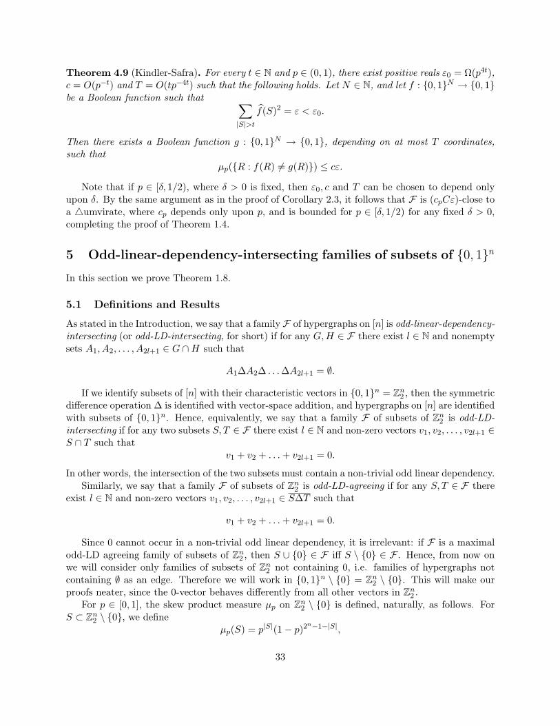
Theorem 4.9 (Kindler-Safra). For every t ∈ N and p ∈ (0, 1), there exist positive reals ε0 = Ω(p4t),c = O(p−t) and T = O(tp−4t) such that the following holds. Let N ∈ N, and let f : 0, 1N → 0, 1be a Boolean function such that ∑

|S|>t

f(S)2 = ε < ε0.

Then there exists a Boolean function g : 0, 1N → 0, 1, depending on at most T coordinates,such that

µp(R : f(R) 6= g(R)) ≤ cε.

Note that if p ∈ [δ, 1/2), where δ > 0 is fixed, then ε0, c and T can be chosen to depend onlyupon δ. By the same argument as in the proof of Corollary 2.3, it follows that F is (cpCε)-close toa 4umvirate, where cp depends only upon p, and is bounded for p ∈ [δ, 1/2) for any fixed δ > 0,completing the proof of Theorem 1.4.

5 Odd-linear-dependency-intersecting families of subsets of 0, 1n

In this section we prove Theorem 1.8.

5.1 Definitions and Results

As stated in the Introduction, we say that a family F of hypergraphs on [n] is odd-linear-dependency-intersecting (or odd-LD-intersecting, for short) if for any G, H ∈ F there exist l ∈ N and nonemptysets A1, A2, . . . , A2l+1 ∈ G ∩H such that

A1∆A2∆ . . .∆A2l+1 = ∅.

If we identify subsets of [n] with their characteristic vectors in 0, 1n = Zn2 , then the symmetric

difference operation ∆ is identified with vector-space addition, and hypergraphs on [n] are identifiedwith subsets of 0, 1n. Hence, equivalently, we say that a family F of subsets of Zn

2 is odd-LD-intersecting if for any two subsets S, T ∈ F there exist l ∈ N and non-zero vectors v1, v2, . . . , v2l+1 ∈S ∩ T such that

v1 + v2 + . . . + v2l+1 = 0.

In other words, the intersection of the two subsets must contain a non-trivial odd linear dependency.Similarly, we say that a family F of subsets of Zn

2 is odd-LD-agreeing if for any S, T ∈ F thereexist l ∈ N and non-zero vectors v1, v2, . . . , v2l+1 ∈ S∆T such that

v1 + v2 + . . . + v2l+1 = 0.

Since 0 cannot occur in a non-trivial odd linear dependency, it is irrelevant: if F is a maximalodd-LD agreeing family of subsets of Zn

2 , then S ∪ 0 ∈ F iff S \ 0 ∈ F . Hence, from now onwe will consider only families of subsets of Zn

2 not containing 0, i.e. families of hypergraphs notcontaining ∅ as an edge. Therefore we will work in 0, 1n \ 0 = Zn

2 \ 0. This will make ourproofs neater, since the 0-vector behaves differently from all other vectors in Zn

2 .For p ∈ [0, 1], the skew product measure µp on Zn

2 \ 0 is defined, naturally, as follows. ForS ⊂ Zn

2 \ 0, we defineµp(S) = p|S|(1− p)2

n−1−|S|,

33

i.e. the probability that a p-random subset of Zn2 \ 0 is equal to S, and if F is a family of subsets

of Zn2 \ 0, we define

µp(F) =∑S∈F

µp(S).

We will work mostly with the uniform measure µ1/2, which we will write as µ.A Schur triple of vectors in Zn

2 \ 0 is a set of three vectors x, y, z such that x + y = z(i.e. x + y + z = 0) — equivalently, a linearly dependent set of size 3. We say that a family T ofsubsets of Zn

2 \ 0 is a Schur junta if there exists a Schur triple x, y, x + y such that T consistsof all subsets of Zn

2 \ 0 with prescribed intersection with x, y, x + y. Similarly, we say that Tis a Schur-umvirate if there exists a Schur triple x, y, x + y such that T consists of all subsets ofZn

2 \ 0 containing x, y, x + y.An odd linear dependency will be the analogue of an odd cycle. We have the following:

Theorem 5.1. If F is an odd-LD-agreeing family of subsets of Zn2 \ 0 then

µ(F) ≤ 1/8.

Equality holds if and only if F is a Schur junta. Moreover, there exists a constant c such that forany ε > 0, if F is an odd-LD-agreeing family of subsets of Zn

2 \ 0 with µ(F) > 18 − ε, then there

exists a Schur junta T such thatµ(T ∆F) ≤ cε.

A similar result holds for the skew product measures:

Theorem 5.2. • [Extremal Families] Let p ≤ 1/2. If F is an odd-LD-intersecting family ofsubsets of Zn

2 \ 0, thenµp(F) ≤ p3.

Equality holds if and only if F is a Schur-umvirate.

• [Stability] There exists a constant c such that for any ε ≥ 0, if F is an odd-LD-intersectingfamily with µp(F) ≥ p3 − ε then there exists a Schur-umvirate T such that

µp(T ∆F) ≤ cε.

We may deduce Theorem 1.4 from this by ‘lifting’ a family of graphs to a family of subsets ofZn

2 \ 0, in the obvious way. In detail, let F be an odd-cycle-intersecting family of graphs. Let

H = F ∪ S : F ∈ F , S ⊂ 0, 1n \ ([n](2) ∪ 0);

then µp(H) = µp(F), and H is odd-LD-intersecting, since an odd cycle is lifted to an odd lineardependency.

It seems impossible to deduce Theorem 5.1 from Theorem 1.4, so Theorem 5.1 is in some sense abona-fide generalization. The calculations required to prove Theorem 5.1 require one extra specialcase to be checked, but are in some ways simpler and more elegant, suggesting that this is thecorrect setting for our ideas. Indeed, we make crucial use of the fact that the ground set (as wellas its power set) lives inside a vector space over Z2.

We will focus on the case of the uniform measure, Theorem 5.1, and only mention briefly howto prove Theorem 5.2.

34

5.2 Cayley operators

First, some preliminaries. If S ⊂ Zn2 \ 0, we write rank(S) = dim(Span(S)) for the dimension of

the subspace spanned by S. Let I(S) = v ∈ S : v /∈ Span(S \ v) be the subset of S consistingof vectors which do not appear in any linear dependency of S, and let m(S) = |I(S)|. We writeJ(S) = S \ I(S) for the union of the linearly dependent subsets of S.

For x, y ∈ Zn2 , we write

〈x, y〉 =n∑

i=1

xiyi

for the standard bilinear form on Zn2 . If S ⊂ Zn

2 , we write

S⊥ = x ∈ Zn2 : 〈x, v〉 = 0.

Then S⊥ is a subspace of Zn2 , satisfying dim(S⊥) + dim(Span(S)) = n.

Recall that an affine subspace of a vector space V is a subset of V of the form U + a, where Uis a vector subspace of V , and a ∈ V — i.e., it is a translate of a subspace. If U has dimension d,then U + a is also said to have dimension d. If V has dimension n, an affine subspace of V withdimension n− 1 is called an affine hyperplane of V .

We will need the following easy lemma:

Lemma 5.3. If S = v1, . . . , vd ⊂ Zn2 is linearly independent, then for any r1, . . . , rd ∈ 0, 1, the

setA := x ∈ Zn

2 : 〈vi, x〉 = ri ∀i ∈ [d]

is a translate of S⊥, and is therefore an affine subspace with dimension n− d.

Proof : For each i ∈ [d] choose a vector yi ∈ (S \ vi)⊥ \ S⊥. Note that (S \ vi)⊥ is a subspaceof dimension n − d + 1, and S⊥ is a subspace of dimension n − d, so (S \ vi)⊥ \ S⊥ is certainlynonempty. Moreover, 〈yi, vj〉 = δi,j . Let

a =d∑

i=1

riyi;

thenA = a + S⊥,

as required.

In particular, if w ∈ Zn2 \ 0 then a set of the form

Aw := v ∈ Zn2 : 〈v, w〉 = 1

is an affine hyperplane. The following simple observation drives our whole approach:

Lemma 5.4. An affine hyperplane of the form

Aw = v ∈ Zn2 : 〈v, w〉 = 1 (w ∈ Zn

2 \ 0)

contains no odd linear dependency.

35

Proof : If v1, . . . , v2l+1 ∈ Aw then

〈2l+1∑i=1

vi, w〉 =2l+1∑i=1

〈vi, w〉 = 1,

so∑2l+1

i=1 vi 6= 0.

This motivates the following

Definition 5.5. A hyperplane subset is a subset of some Aw, where w ∈ Zn2 .

Observe that if A is a hyperplane subset, F is odd-LD-agreeing, and S ∈ F , then S ⊕ A /∈ F .A hyperplane subset will be the analogue of a bipartite graph. Indeed, a bipartite graph G withbipartition (X, Y ) is a subset of Aw if we define wi = 1i ∈ X.

If w is a vector chosen uniformly at random from Zn2 , and S ⊂ 0, 1n, we write YS = |S ∩Aw|.

Note that S ∩ Aw is the analogue of a random cut in a graph. Indeed, if S ⊂ [n](2), i.e. S is agraph, then S ∩Aw is precisely a random cut in S, and YS is the number of edges in a random cutin S. We write QS(X) for the probability-generating function of the random variable YS .

We now have a Cayley graph on Z0,1n\02 (rather than Z[n](2)

2 ), where the generating set isA : A is a hyperplane subset.

Definition 5.6. A linear operator A on real-valued functions on Z0,1n\02 will be called Odd-

Linear-Dependency-Cayley, or OLDC for short, if it has the following two properties:

1. If F is an odd-LD-agreeing family, and f is its characteristic function, then

f(S) = 1 ⇒ Af(S) = 0.

2. The Fourier-Walsh basis is a complete set of eigenfunctions of A.

The vector of eigenvalues of an OLDC operator, indexed by the subsets of 0, 1n \ 0, will becalled an OLDC spectrum.

We have the following analogue of Corollary 2.9:

Corollary 5.7. Let w be a uniform random vector in Zn2 , i.e. where each component is indepen-

dently chosen to be 0 or 1 with probability 1/2. Let

Aw = v ∈ Zn2 : 〈v, w〉 = 1.

For any subset S ⊂ Zn2 , let

qi(S) = Pr[|S ∩Aw| = i],

and for any set R ⊂ Zn2 with no non-trivial odd linear dependency, let

qR(S) = Pr[(S ∩Aw)∼=R],

where H ∼=R means that there is a linear isomorphism of Zn2 mapping H to R, and all probabilities

are over the choice of the random vector w. Then for any integer i,

λS = (−1)|S|qi(S)

is an OLDC spectrum, and for any set R ⊂ Zn2 with no non-trivial odd linear dependency,

(−1)|S|qR(S)

is an OLDC spectrum.

36

5.3 Construction of the OLDC spectrum

Note that if S = v1, . . . , vd is linearly independent, then 〈vi, w〉 : i ∈ [d] is an independentsystem of Bin(1, 1/2) random variables. To see this, observe that for any r1, . . . , rd ∈ 0, 1, byLemma 5.3,

w ∈ Zn2 : 〈vi, w〉 = ri ∀i ∈ [d]

is an affine subspace of Zn2 of dimension n− d, and therefore has size 2n−d.

It follows that for each v ∈ I(S), the Bin(1, 1/2) random variable 〈v, w〉 is independent ofthe system 〈v′, w〉 : v′ ∈ S \ v. Hence, for any S, if I(S) = v1, . . . , vm and J(S) = J =u1, . . . , ul then

YS =m∑

i=1

Yvi + YJ .

writeQJ(X) =

∑i≥0

aiXi;

note that a1 = 0. We have

QS(X) = (12 + 1

2X)mQJ(X)= 1

2m (1 + X)m(a0 + a2X2 + a3X

3 + . . .)= 1

2m

(1 + mX +

(m2

)X2 +

(m3

)X3 + . . .

) (a0 + a2X

2 + a3X3 + . . .

)= 1

2m

(a0 + ma0X +

((m2

)a0 + a2

)X2 +

((m3

)a0 + ma2 + a3

)X3 + R(X)X4

), (8)

where R(X) ∈ Q[X]; this is the exact analogue of (5).The ‘same’ spectrum which worked before turns out to work in the new setting also:

Claim 8. Let Λ(1) be the OLDC spectrum described by

λ(1)S = (−1)|S|

[q0(S)− 5

7q1(S)− 1

7q2(S) +

328

q3(S)]

,

Then

• λ(1)∅ = 1.

• λ(1)min = −1/7.

• Λ(1)min consists of all singletons, all sets of size 2, all linearly independent sets of size 4, and

all sets of the form x, y, z, x + y, x + z.

• For all S 6∈ Λ(1)min it holds that λ

(1)S ≥ −1/7 + γ′, with γ′ = 1/56.

We remark that sets of size 2 are the analogue of 2-forests, linearly independent sets of size 4are the analogue of 4-forests, and x, y, z, x + y, x + z is the analogue of K−

4 . All sets of size 2(and all linearly independent sets of size 4) are isomorphic, so unlike in the graph case, we neednot distinguish between them.

In order to prove Claim 8, we need the following generalization of Lemma 3.1:

37

Lemma 5.8. Let S be a set of vectors.

1. q0(S) = 2− rank(S).

2. q1(S) = m(S)q0(S) = m(S)2− rank(S).

3. If there exists i ∈ [n] such that |v ∈ S : v(i) = 1| is odd, then qk(S) ≤ 1/2 for any k ≥ 0.

4. For any odd k, qk(S) ≤ 1/2.

5. Always q2(S) ≤ 3/4.

Proof : We follow the items of the lemma.

1. Observe that q0(S) is the probability that w lies in the subspace S⊥, which has dimensionn− rank(S), and therefore size 2n−rank(S), proving 1.

2. Observe that |S ∩Aw| = 1 if and only if w ∈ (S \ v)⊥ \S⊥ for some v ∈ I(S): if v ∈ S ∩Aw

participates in some linear dependency v =∑

vi, then linearity of the inner product impliesthat not all the vi can be outside Aw. The sets (S \ v)⊥ \S⊥ : v ∈ I(S) are disjoint, andeach has size 2n−rank(S), proving 2.

3. LetTk = w ∈ 0, 1n : |S ∩Aw| = k.

Observe that for any w ∈ Tk, w + ei /∈ Tk, where ei denotes the vector (0, 0, . . . , 0, 1, 0, . . . , 0)with a 1 in the ith place (cf. the corresponding part in the proof of Lemma 3.1). It followsthat |Tk| ≤ 2n−1, i.e. qk(S) ≤ 1/2, proving 3.

4. By item 3, we may assume that for each i ∈ [n], |v ∈ S : v(i) = 1| is even. But then forany w ∈ Zn

2 ,∑

s∈S〈s, w〉 = 0 (since every w(i) is summed an even number of times), andtherefore |s ∈ S : 〈s, w〉 = 1| is even. Hence qk(S) = 0 for any odd k ∈ N, proving 4.

5. The average size of |S ∩Aw| is |S|/2, and therefore

|S|/2 =∑

k

kqk(S) < 2q2(S) + (1− q2(S))|S| = |S|+ (2− |S|)q2(S);

the inequality is strict because q0(S) > 0. Hence,

q2(S) <|S|

2(|S| − 2)=

12

+1

|S| − 2.

Therefore q2(S) < 3/4 if |S| ≥ 6. Assume from now on that |S| ≤ 5.

By item 3, we may assume that for each i ∈ [n], |v ∈ S : v(i) = 1| is even, and therefore∑v∈S v = 0. Let T ⊂ S be the smallest linearly dependent subset of S. Since |S| ≤ 5, T

must be of the form x, y, x + y, x, y, z, x + y + z, or x, y, z, v, x + y + z + v. Since Ssums to zero, S \ T must also sum to zero, but |S \ T | ≤ 2, and no set of size 1 or 2 sums tozero. Hence, S \ T = ∅, i.e. S = T . One may check that

q2(x, y, x + y) = q2(x, y, z, x + y + z) = 3/4, q2(x, y, z, v, x + y + z + v) = 5/8,

proving 5.

38

We also need a counterpart of Lemma 3.2:

Lemma 5.9. Let S be a set of vectors.

1. We have q0(∅) = 1, q0(x) = 1/2, and q0(S) ≤ 1/4 for all other sets.

2. If m(S) = 0 and |S| is odd, then either q0(S) ≤ 1/16 or S is of the form

x, y, x + y, x, y, z, x + y, x + z, or x, y, z, x + y, y + z, x + z, x + y + z.

3. Either J(S) = ∅ or a0 ≤ 1/4.

Proof : 1. If S 6= ∅, x then rank S ≥ 2, so the item follows from Lemma 5.8(1).

2. If rank(S) ≥ 4 then item 1 implies that q0(S) ≤ 1/16. If rank(S) ≤ 3, the only possibilitiesfor S are those listed.

3. If J(S) 6= ∅ then rank(J(S)) ≥ 2, since there is no linear dependency in x, so the itemfollows from item 1.

We note that in item 2, the first possibility corresponds to a triangle, and the second to a K−4 . The

third possibility has no graph counterpart.As before, these lemmas enable us to prove Claim 8:

Proof of Claim 8: The proof of Claim 2 relied on equation (5) and Lemmas 3.1 and 3.2. Inorder to prove Claim 8, we replace those by equation (8) and Lemmas 5.8 and 5.9. The proof goesthrough line-by-line if we replace G with S, m with m(S) and H with J(S). The proof uses theunconditional estimates of Lemma 3.1 and the conditional estimates of Lemma 3.2; these carrythrough in the present setting. In a few places, f(G) was explicitly calculated for some graphs;those are either forests, or the exceptional graphs of Lemma 3.2(2). In the present setting, werequire exactly the same explicit calculations for the corresponding sets, and there is just one otherexceptional structure to deal with,

S = x, y, z, x + y, x + z, y + z, x + y + z,

which hasQS(X) =

18

+78X4.

In this case, we explicitly calculate f(S) = 1/8 = 1/7− 1/56. This completes the proof of Claim 8.

We have the following analogue of Claim 3:

Claim 9. Let Λ(2) be the OLDC spectrum described by

λ(2)S = (−1)|S|

[∑qI(S)− q(G)

]where I denotes a linearly independent set of size 4, and denotes the set a, b, c, a+ b+ c. Then

39

1. λ(2)S = 0 for all S with |S| ≤ 3.

2. λ(2)S = 1/16 if S is a linearly independent set of size 4.

3. λ(2)x,y,z,x+y,x+z = 1/8.

4. |λ(2)S | ≤ 1 for all S.

Proof : We follow the items of the claim:

1. Clear.

2. For any linearly independent sets I, I ′ of size 4, qI(I ′) = q4(I ′) = 1/16. Also q(I ′) = 0.

3. Let S = x, y, z, x + y, x + z. Clearly, qI(S) = 0 for any linearly independent set I of size4. Note that the only subset of S isomorphic to a, b, c, a + b + c is y, z, x + z, x + z, andtherefore q(S) = 1/8, proving 3.

4. Finally, |λ(2)(S)| is the difference between two probabilities, hence is at most 1.

Exactly the same argument as before now shows that if F is an odd-LD-agreeing family ofsubsets of 0, 1n \0, then µ(F) ≤ 1/8. If F is odd-LD-intersecting, we may deduce from Lemma2.4 that equality holds only if F consists of all families of subsets containing a fixed Schur triplex, y, x + y. If F is an odd-LD-agreeing family of subsets of 0, 1n \ 0, we may deduce usingthe same monotonization argument as in Lemma 2.7 that equality holds only if F is a Schur junta.Stability follows by the same argument as before.

5.4 p < 1/2

We now outline briefly how the skew-measure analogue, Theorem 5.2, can be proved using thetechnique of section 4. This time the proof of the main claim, Claim 5, relies also on Lemma 4.7.It is easy to extend this lemma to the current setting:

Lemma 5.10. Let S be a set of vectors.

1. If m(S) = 1 and |S| > 1 then |S| ≥ 4.

2. If m(S) = 0 and |S| ≤ 5, then S is of the form

x, y, x + y, x, y, z, x + y + z, x, y, z, w, x + y + z + w, or x, y, z, x + y, x + z.

Proof : 1. The smallest linear dependency is x, y, x + y.

2. Easy enumeration. Note that x, y, z, x + y, x + y + z is isomorphic to the last member inthe list.

All sets in item (2) correspond to graphs: a triangle, C4, C5, and K−4 , respectively. Therefore

the only new case to check is the extra case in Lemma 5.9(2). In this case also, we have λG >−p3/(1− p3), and so Claim 5 remains true in the current setting. This leads to a proof of Theorem5.2.

40

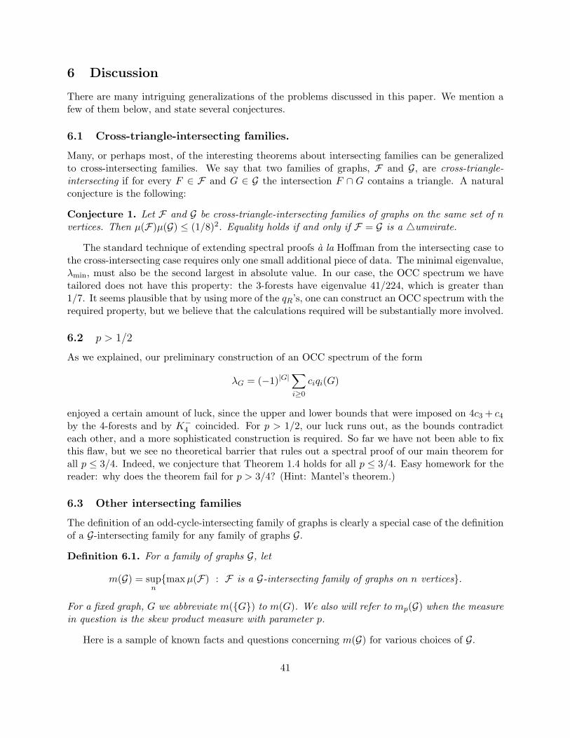
6 Discussion

There are many intriguing generalizations of the problems discussed in this paper. We mention afew of them below, and state several conjectures.

6.1 Cross-triangle-intersecting families.

Many, or perhaps most, of the interesting theorems about intersecting families can be generalizedto cross-intersecting families. We say that two families of graphs, F and G, are cross-triangle-intersecting if for every F ∈ F and G ∈ G the intersection F ∩ G contains a triangle. A naturalconjecture is the following:

Conjecture 1. Let F and G be cross-triangle-intersecting families of graphs on the same set of nvertices. Then µ(F)µ(G) ≤ (1/8)2. Equality holds if and only if F = G is a 4umvirate.

The standard technique of extending spectral proofs a la Hoffman from the intersecting case tothe cross-intersecting case requires only one small additional piece of data. The minimal eigenvalue,λmin, must also be the second largest in absolute value. In our case, the OCC spectrum we havetailored does not have this property: the 3-forests have eigenvalue 41/224, which is greater than1/7. It seems plausible that by using more of the qR’s, one can construct an OCC spectrum with therequired property, but we believe that the calculations required will be substantially more involved.

6.2 p > 1/2

As we explained, our preliminary construction of an OCC spectrum of the form

λG = (−1)|G|∑i≥0

ciqi(G)

enjoyed a certain amount of luck, since the upper and lower bounds that were imposed on 4c3 + c4

by the 4-forests and by K−4 coincided. For p > 1/2, our luck runs out, as the bounds contradict

each other, and a more sophisticated construction is required. So far we have not been able to fixthis flaw, but we see no theoretical barrier that rules out a spectral proof of our main theorem forall p ≤ 3/4. Indeed, we conjecture that Theorem 1.4 holds for all p ≤ 3/4. Easy homework for thereader: why does the theorem fail for p > 3/4? (Hint: Mantel’s theorem.)

6.3 Other intersecting families

The definition of an odd-cycle-intersecting family of graphs is clearly a special case of the definitionof a G-intersecting family for any family of graphs G.

Definition 6.1. For a family of graphs G, let

m(G) = supnmax µ(F) : F is a G-intersecting family of graphs on n vertices.

For a fixed graph, G we abbreviate m(G) to m(G). We also will refer to mp(G) when the measurein question is the skew product measure with parameter p.

Here is a sample of known facts and questions concerning m(G) for various choices of G.

41

• It was observed by Noga Alon [2] that for every star forest G, m(G) = 1/2. He furtherconjectured that there is an ε > 0 so that for every G which is not a star forest m(G) < 1/2−ε,and pointed out that this holds for all non-bipartite graphs G and that it suffices to provethe conjecture for P3, the path with 3 edges.

An intriguing fact is that the simplest guess, m(P3) = 1/8 (conjectured in [4]), is false.Demetres Christofides [3] has constructed a P3-intersecting family of graphs on 6 vertices,with measure 17/128 > 1/8.

• The obvious conjecture generalizing our main theorem is that if Gk denotes the family ofnon-k-colorable graphs, then mp(Gk) = p(k+1

2 ) for all p ≤ 2k−12k , with equality only for Kk+1-

umvirates. It is quite plausible that, at least for small values of k and p = 1/2, this conjecturewill be amenable to our methods.

• It seems to us, perhaps for lack of imagination, that the 4umvirate might be extremal notonly for odd-cycle-intersecting families, but also for the more general case of cycle-intersectingfamilies. If true, this would hold only for p ≤ 1/2. An indication that this may be asignificantly harder question is the fact that for p = 1/2 there is a neck-to-neck race formaximality between the 4umvirate and the family of all graphs with at least 1

2

(n2

)+ 1

2nedges, and to settle the result one needs to consult the table of the normal distribution.Moreover, the generalization of this statement to non-uniform hypergraphs is false. A cycle-intersecting family of graphs corresponds to a linear-dependency-intersecting family of subsetsof Zn

2 \ 0, but it is easy to construct such a family with measure 1/2− o(1). (Take all setsof vectors with cardinality at least 2n−1 + (n + 1)/2. The intersection of any two is a set ofat least n + 1 vectors, and is therefore linearly dependent. Standard estimates show that thisfamily has measure 1/2− o(1).)

There are many other interesting structures (other than a graph structure) that one may imposeon the ground set. An example studied in [4] is the cyclic group Zn of integers modulo n. ForB ⊂ Zn, we say that a family F of subsets of Zn is B-translate-intersecting if the intersection ofany two sets in F contains a translate of B. The authors conjecture that a B-translate-intersectingfamily of subsets of Zn has size at most 2n−|B|. They prove this in the case where B is an interval;Paul Russell [15] has given a different, algebraic proof. Furedi, Griggs, Holzman and Kleitman [9]have proved it in the case |B| = 3. Griggs and Walker [10] prove that for each B, the conjectureholds for infinitely many values of n. For most configurations B, the question (for all n) remainsopen.

6.4 Connection to entropy?

The OCC spectrum that we constructed can be expressed in the form∑

cBAB, where the sum ofthe coefficients cB is 1. However, this is not a convex combination, as some of the coefficients arenegative. We observe that if we restrict ourselves to non-negative coefficients, our proof methodcannot give a bound better than 1/4. At the risk of falling prey to mundane numerology, we cannothelp but wonder if there is a connection to the bound of 1/4 that one gets using entropy. We raisethis question due to the other superficial resemblances between our approach and that of [4].

Acknowledgements: We would like to thank Vera Sos and Noga Alon for useful conversations.

42

References

[1] Rudolf Ahlswede and Levon H. Khachatrian. The complete intersection theorem for systemsof finite sets. Eur. J. Comb., 18(2):125–136, 1997.

[2] N. Alon. Personal communication, Erzsebet Bridge, Buda, August 1999.

[3] D. Christofides. Personal communication, August 2010.

[4] Fan R. K. Chung, Ronald L. Graham, Peter Frankl, and James B. Shearer. Some intersectiontheorems for ordered sets and graphs. J. Comb. Theory, Ser. A, 43(1):23–37, 1986.

[5] David Ellis, Ehud Friedgut, and Haran Pilpel. Intersecting families of permutations. To appearin Journal of the American Mathematical Society.

[6] Paul Erdos, Chao Ko, and Richard Rado. Intersection theorems for systems of finite sets.Quart. J. Math., 2:313–320, 1961.

[7] Peter Frankl. The shifting technique in extremal set theory. In Surveys in Combinatorics,volume 123 of Lond. Math. Soc. Lect. Note Ser., pages 81–110. 1987.

[8] Ehud Friedgut. On the measure of intersecting families, uniqueness and stability. Combina-torica, 28(5):503–528, 2008.

[9] Z. Furedi, J.R. Griggs, R. Holzman, and D.J. Kleitman. Representations of families of triplesover gf(2). J. Comb. Theory, Ser. A, 53(2):306–315, 1990.

[10] Jerrold R Griggs and James W Walker. Anticlusters and intersecting families of subsets.Journal of Combinatorial Theory, Series A, 51(1):90–103, 1989.

[11] A. J. Hoffman. On eigenvalues and colorings of graphs. In Graph Theory and its Applications,Proc. Advanced Sem., Math. Research Center, Univ. of Wisconsin, Madison, Wis., pages 79–91. academic Press, New york, 1969.

[12] D.G. Hook and P.R. McAree. Using Sturm sequences to bracket real roots of polynomialequations. In A. Glassner, editor, Graphic Gems I, pages 416–422. Academic Press, 1990.

[13] Guy Kindler and Shmuel Safra. Noise-resistant boolean-functions are juntas. Manuscript,http://www.cs.huji.ac.il/ gkindler/papers/noise-stable-r-juntas.ps, March 2004.

[14] Noam Nisan and Mario Szegedy. On the degree of boolean functions as real polynomials.Computational Complexity, 4:301–313, 1994.

[15] Paul A. Russell. Families intersecting on an interval. Discrete Mathematics, 309(9):2952–2956,2009.

[16] R. M. Wilson. The exact bound in the Erdos-Ko-Rado theorem. Combinatorica, 4(2-3):247–257, 1984.

43