trends in materials simulation: a molecular … in materials simulation: a molecular dynamics...

1

Trends in Materials Simulation:

A Molecular Dynamics Miscellany

Florian Müller-Plathe (www.theo.chemie.tu-darmstadt.de)

2

Polymers: Scales & MethodsReview: FMP, Soft Materials 1, 1 (2003)

length

tim

e

Quantum

chemistry

Atomistic

simulation

Coarse-grained model

Soft fluid

Finite

element

Polymer-

isation

Solvation,

permeation

Crystallisation,

rheology

MorphologyProcessing

3

Polymers: Structure and Properties

• Chemistry

rubber brittle

• Tacticity

insoluble water-soluble

• Sequence

engineering plastic synthetic rubber

• Topology

shopping bag bullet-proof vest

CH3H3C CH3H3C CH3H3C

ClCl ClCl Cl

Cl

O

CH2OH

O

HO

HO

O

O

CH2OH

HO

HO

OO

CH2OH

O

HO

HO

O

O

CH2OH

HO

OH

O

S-S-S-S-B-B-B-B S-B-S-S-B-S-B-B

4

Multiscaling and Dynamics

Multiscale Methods

Structure-basedcoarse graining

Successes and failures

Transport properties

Reverse nonequilibriummolecular dynamics

Attempt of a synthesis:

Dynamics of coarse-grained models


5

• Transport coefficient

flux, flow, current, ...

driving force, field,

thermodynamic force

Transport Coefficients

EJ

• Non-equilibrium situation: steady-state, periodic, ...

• Linear response: small perturbation

• Isotropic medium: liquid, melt, ...

6

Linear response

• Coupled energy and

mass

Ludwig 1856, Soret 1879

• General Onsager 1931

energy and mass

• Mass Berthollet 1803

Fick 1854

• Charge Ohm 1826

• Energy Fourier 1822

• Momentum

J D c z1 ( / )

I R z( / ) ( / )1

J T zQ ( / )

J p v z( ) ( / )

[ ]xy

J D w z

S w w T zT

1 12 1

1 11

[ ( / )

( ) ( / )]

J XL

J LT

LT

T

TQ1 11 1 2

7

Equilibrium

Einstein

Green-Kubo

Non-equilibrium

Steady-state

J( ,k )

Boundary-driven Synthetic

Periodic

J( ,k)

-F

F

Calculation of Transport

Coefficients by MD

8

Traditional NEMD Reverse NEMD

J E

calculate impose

J E

calculateimpose

Examples:

• shear viscosity

• thermal conductivity

• Soret coefficient ST

1st Ingredient:

Reverse cause and effect

9

energy transport (unphysical)

Heat flow

zdTdJQ /

0 2 4 6 8 100.60

0.65

0.70

0.75

0.80

slab numberte

mp

era

ture

F. Müller-Plathe, J. Chem. Phys. 106, 6082 (1997)

Fourier’s law:

Thermal Conductivity

Repeat periodically, wait for steady state

10

Find hottest particle in

the cold region and

coldest particle in the

hot region

Swap their

velocities v

If m1=m2: no change in total linear momentum

no change in total kinetic energy

no change in total energy

1

2z

What we want

Hot

Cold

1

2

2nd Ingredient:

Unphysical velocity exchange

11

0.0 0.5 1.0 1.5 2.0 2.5 3.0 3.5260

270

280

290

300

310

320

330

340

Tem

pera

ture

(K

)

z (nm)

rigid SPC/E

flexible SPC/EThermal conductivity

(Wm-1K-1)

rigid 0.81 0.01

flexible 0.95 0.01

experiment 0.607M. Zhang, E. Lussetti, L.E.S. de Souza, F. Müller-Plathe,

J. Phys.Chem. B 109, 15060 (2005).

• Calculate temperature profile T(z)

• Obtain gradient dT/dz

• Fourier’s law

dzdT

J q

Analyse

12

0.1 10.1

1

Exp

eri

me

nt

Simulation

Thermal conductivity / W K-1m

-1

H2O

Ar

c-hexanebenzenen-hexane

polyamide-6,6

M. Zhang, E. Lussetti, L.E.S. de Souza, F. Müller-Plathe,

J. Phys.Chem. B 109, 15060 (2005).

Thermal conductivity

of molecular liquids

13

Thermal Conductivity of Polyamide-6,6

Simulation Experiment

W/K m W/K m

amorphous (1.07 g/cm3)

(flexible model) 0.33-0.35 ~0.25

(semirigid model) 0.20

stretched amorphous (0.95 g/cm3)

parallel to stretching 0.43

perpendicular 0.20

Enrico Lussetti, Takamichi Terao, FMP, J. Phys. Chem. B 111,

11516-11523 (2007); Phys. Rev. E 75, 057701 (2007).

| FB Chemie | Prof. Dr. Florian Müller-Plathe | 14

Carbon nanotubesM. Alaghemandi, E. Algaer, M. C. Böhm, FMP,

Nanotechnology 20, 115704 (2009).

depends on tube length

power law

Breakdown of Fourier’slaw

Possibly different exponents for short and long tubes.Theory:

= 0.83 → 0.35 J. Wang, J.-S. Wang, Appl. Phys. Lett. 88, 111909 (2006)

Chirality of tube unimportant

8.05.0L

10 100 40010

100

1000

therm

al conductivity

(W

m-1K

-1)

tube length (nm)

(5,5)

(10,0)

(7,7)

(17,0)

(10,10)

(15,15)

(20,20)

54.0L

77.0L

| FB Chemie | Prof. Dr. Florian Müller-Plathe | 15

Anisotropy of thermal conductivity

CNT crystal

||: 100 – 1000 W m-1K-1

(better than metal)

: 0.14 W m-1K-1

(worse than polymer)

CNT bundle

||: 100 – 1000 W m-1K-1

: 0.09 W m-1K-1

Fast parallel mechanism (phonons) ↔

slow lateral mechanism (collisions between neighbouring tubes).

y

x

Multiwall nanotube 10 nm

||: 21 W m-1K-1

: 0.24 W m-1K-1

Extreme anisotropies!

16

vx

x

z

-vxA

y

Lx

Ly

jz(px)

L z

x

z

m o m e n tu m flu x(p h y sica l )

v x

m o m e n tu mtr a n sfe r(u n p h y sic al )

F. Müller-Plathe, Phys. Rev. E 59, 4894-4899 (1999).

Shear viscosity

17

Find 2 particles that

move against the

current

Swap their

vx

If m1=m2: no change in total linear momentum

no change in total kinetic energy

no change in total energy

→ no thermostat!

1

2

1

2

x

z

What we want

Exchange of velocity component

18

• What have we done?

• Impose a flux of transverse linear momentum J(p )

= apply a shear force

• higher perturbation = swap velocities more often

• What still needs to be done?

• Measure shear rate:

Measure profile of flow velocity, determine dv /dz

• Viscosity is proportionality constant

dz

dvpJ

Shear viscosity

19

1200300

153

0 3 6 9 12 15 18z /

-0.12

-0.08

-0.04

0.00

0.04

0.08

0.12

vx (

m /

)1/2

60

Lennard-Jones liquid near triple point

Vel

oci

ty

Strong perturbation

Weak perturbation

Velocity profiles

20

-4 -3 -2 -1 0

log10[( vx / z) ( /m 2)-1/2]

-3

-2

-1

0

log

10[ j z

( px)

(3/

)]NVE

NVTslope 1


Velocity gradient = shear rate

Tra

nsv

erse

mom

entu

m f

lux

= s

hea

r fo

rce

Linear response holds

21

-3 -2 -1 01.5

2.0

2.5

3.0

3.5

4.0

2(

m)-1

/2

log10[ jz(px) (3/ )]

lit.

constant temperature

constant energy


Shear viscosity of the

Lennard-Jones fluid

22

Recall:

• Total energy is conserved: microcanonical (NVE)

But:

• Viscous flow friction heating !!!

Question:

• How is the heat removed?

Answer: Maxwell demon

• Undirected motion (heat) Directed motion (flow)

• Cooling in exchange regions

Proof: temperature profile

• Ekin(total) = Ekin(temperature) + Ekin(flow)

• Peculiar velocity ui = vi - v defines temperature

Viscous flow

without viscous heating?

23

0.7

0.75

0.8

0.85

0.9

0.95

1

1.05

0 5 10 15 20

z/sigma

(Heat)

/ (

To

tal

Ek

in)

W=3

W=15

High shear

Temperature profile from

peculiar velocities

24

P. Bordat, F. Müller-Plathe,

J. Chem. Phys. 116, 3362 (2002)

Molecular Liquids

252.6 2.8 3.0 3.2 3.4 3.6

1

10

100

5%

1%

10%30%

60%

Sh

ea

r vis

co

sity

(cP

)

1000/T (1/K)

Aqueous solutions of saccharose

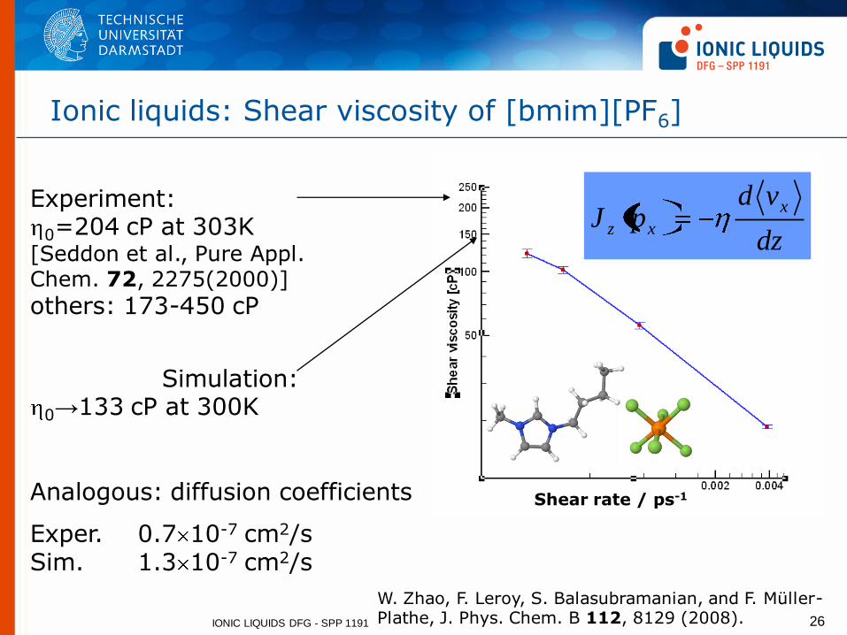
IONIC LIQUIDS DFG - SPP 1191 26

Ionic liquids: Shear viscosity of [bmim][PF6]

Simulation:

0→133 cP at 300K

Analogous: diffusion coefficients

Exper. 0.7 10-7 cm2/sSim. 1.3 10-7 cm2/s

W. Zhao, F. Leroy, S. Balasubramanian, and F. Müller-Plathe, J. Phys. Chem. B 112, 8129 (2008).

Experiment:

0=204 cP at 303K[Seddon et al., Pure Appl. Chem. 72, 2275(2000)]

others: 173-450 cP

Shear rate / ps-1

dz

vdpJ

x

xz

27


Multiscale Methods








28

Atomistic Model – Bridge Incomplete

29

Polymers: Scales & MethodsReview: FMP, Soft Materials 1, 1 (2003)

length

tim

e

Quantum

chemistry

Atomistic

simulation

Coarse-grained model

Soft fluid

Finite

element

Polymer-

isation

Solvation,

permeation

Crystallisation,

rheology

MorphologyProcessing

30

Coarse-grained Force Field

~10 atoms → 1 superatom

1000-100000 times cheaper

Effective interactions:“bonds”, “angles”, non-bonded

Systematic coarse-graining:

• interactions as realistic as possible

• model is material-specific

• no generic “bead-and-spring”model

Reviews: F. Müller-Plathe, ChemPhysChem 3, 754 (2002); Soft Materials 1, 1 (2003).

31

Coarse Graining

Objectives for coarse-grained model:

• Simpler than atomistic model: ~10 real atoms → 1 “superatom”

• Material-specific

• Reproduce structure of atomistic model

Atomistic simulation Coarse-grained model

Structure

0.2 0.4 0.6 0.8 1.0 1.2 1.40.0

0.2

0.4

0.6

0.8

1.0

1.2

1.4

RD

F

Distance (nm)

Target

Best fit LJ 6-9

Best fit 6-8-10-12

BondAngle

Torsion

32

1st Example: Poly(vinyl alcohol)

• Polymer in the melt

• 48 decamers

• Use:

• Packaging: O2 barrier

• Fishing nets: same refractive index as water

• Pervaporation membranes:

remove water from organic solvents

CH2 CH2 CH2 CH2

CHCH CH

OHOH OH

33

Coarse-Graining PVA: Angles

OH

HO

OH

OH

60 90 120 150 180

0.000

0.005

0.010

0.015

0.020

0.025

0.030

0.035

Dis

trib

ution (

arb

. units)

Angle (degrees)

Distribution from

atomistic simulation

60 90 120 150 1800

1

2

3

4

5

6

Pote

ntial of m

ean forc

e (

kT

)

Angle (degrees)

Potential of mean force,

use as potential of

coarse-grained model

)(ln PkT

V

The easy part:

• Stiff degrees of freedom

• Direct Boltzmann inversion

34

Coarse-Graining PVA: Nonbonded

0.2 0.4 0.6 0.8 1.0 1.2 1.40.0

0.2

0.4

0.6

0.8

1.0

1.2

1.4

RD

F

Distance (nm)

Target

Best fit LJ 6-9

Best fit 6-8-10-12

Less easy:

• soft degrees of freedom

• potential of mean force

≠ potential energy

• cannot Boltzmann-invert

directly

35

Iterative Boltzmann Inversion

• Tabulated numerical potential V(r)

• Starting guess V0(r) RDF0(r) RDFtarget(r)

• Potential correction

• Iterate

until Vn(r) RDFn(r) = RDFtarget(r)

• Converges in few iterations

• Density/pressure correction can be added

D. Reith, H. Meyer, FMP, Comput. Phys. Commun. 148, 299 (2002).

r

rkTrVrV

target

001

RDF

RDFln

r

rkTrVrV n

nn

target

1RDF

RDFln

36

Iterative Boltzmann Inversion (2)

[D. Reith, M. Pütz, F. Müller-Plathe, J. Comp.Chem. 24, 1624 (2003)]

37

• Polymer in solution

• 23-mer, Na salt, 2 wt.% in water

• Use:

• Additive in washing powders, detergents, etc.

• Flocculation agent in water treatment

• Disposable nappies

CO2-

CO2-

CO2- CO2

-

Na+

Na+

Na+

Na+

Na+

2nd Example: Poly(acrylic acid)

38

Poly(acrylic acid)

Mapping: coarse-grained superatom

centre of mass of atomistic monomer

Water: effective interaction, viscous medium

Coarse-grained:

23 particles

no H2O

CO2-

CO2-

CO2- CO2

-

Na+

Na+

Na+

Na+

Na+

[D. Reith, B. Müller, FMP, S. Wiegand, J.Chem. Phys. 116, 9100 (2002).]

Atomistic:

209 atoms

3000 H2O

counterions

~ 10000 atoms

39

100 1000 10000

1

10

100

Hyd

rod

yn

am

ic r

ad

ius (

nm

)

Molecular weight (monomers)

Simulation

Dynamic Light Scatt.

Parameterisation

Comparison with Experiment

[D. Reith, B. Müller, F. Müller-Plathe, S. Wiegand, J. Chem. Phys. 116, 9100 (2002).]

ji ijH RNR,

2

111

40

Systems coarse-grained

Polymer melts:

• Poly(vinyl alcohol)D. Reith, H. Meyer, FMP, Macromolecules 34, 2235 (2001).

• Polyisoprenetrans: R. Faller, FMP, Polymer 43, 621 (2002); cis: T. Spyriouni, C. Tzoumanekas, D. Theodorou, FMP, G. Milano, Macromolecules 40, 3876 (2007).

• Amorphous celluloseS. Queyroy, S. Neyertz, D. Brown, FMP, Macromolecules 37, 7338 (2004).

• Atactic polystyreneG. Milano, FMP, J. Phys. Chem. B 109, 18609 (2005).

• Amorphous polyamide-6,6P. Carbone, H. A. Karimi Varzaneh, X.Y. Chen, FMP, J. Chem. Phys. 128, 064904 (2008)

Polymer Solutions

• Poly(acrylic acid)D. Reith, B. Müller, F. Müller-Plathe, S. Wiegand, J. Chem. Phys. 116, 9100 (2002).

• Poly(ethylene oxide)R. Cordeiro, FMP, in preparation.

41

Systems coarse-grained

Non-polymers

• Liquid: Diphenyl carbonateH. Meyer, O. Biermann, R. Faller, D. Reith, FMP, J. Chem. Phys. 113, 6265 (2000).

• Liquid: EthylbenzeneH.-J. Qian, P. Carbone, X. Chen, H. A. Karimi-Varzaneh, C. C. Liew, FMP, Macromolecules 41, 9919 (2008).

• PAMAM dendrimersP. Carbone, F. Negri, FMP, Macromolecules 40, 7044 (2007).

• Ionic liquid: [bmim][PF6]W. Zhao H.A. Karimi Varzaneh, FMP, in preparation.

• Carbon nanotubesG. Illya, H.A. Karimi Varzaneh, FMP, in preparation.

• Phospholipid membranesG. Illya, T.J. Müller, H.A. Karimi Varzaneh, FMP, in preparation.

42

Robust Bridge?

43


Multiscale Methods








44

Challenge #1: Dynamics

• One known case:

polycarbonate

• Temperature dependence

(Vogel-Fulcher)

reproduced after

empirical curve shift

[W. Tschöp, K. Kremer, J. Batoulis, T. Bürger, O. Hahn, Acta Polym. 49, 61

(1998); ibid. 49, 75].

45

Dynamics

Known feature of coarse-grained potentials

• repulsion (excluded volume) softer than atomistic

• less friction

• faster dynamics: higher D, lower

Questions

• Can coarse-grained models be constructed with correct

dynamics?

• Is there a constant scale factor?

46

Viscosity: MW dependence

slope ~ 1.0-1.1

below entanglement

1000 10000

0.1

1

Ze

ro-s

he

ar

Vis

co

sit

y (

cP

)

Molecular Weight (g/mol)

500 K

520 K

540 K Polystyrene

coarse-grained model

X. Chen, P. Carbone, W.L. Cavalcanti, G. Milano, F. Müller-Plathe, Macromolecules 40, 8087 (2007).

47

Viscosity: shear-rate dependence

9 Monomers: zero-shear limit

100 Monomers:

• zero-shear limitnot yet reached

• melt is not Newtonian

X. Chen, P. Carbone, W.L. Cavalcanti, G. Milano, F. Müller-Plathe, Macromolecules 40, 8087 (2007).

48

Chain structure under shear

G. Santangelo, A. di Matteo, F. Müller-Plathe, G. Milano, J. Phys. Chem. B 111, 2765 (2007).X. Chen, P. Carbone, G. Santangelo, A. di Matteo, G. Milano, FMP, Phys. Chem. Chem. Phys. 11, 1977 (2009).

Atomistic structureafter re-insertion ofthe atoms:“backmapping”

n scattering, PS-30

parallel to

stretching

perpendicular to stretching

49

Viscosity: Comparison with Experiment

520 525 530 535 540

1

10

100

Ze

ro-s

he

ar

Vis

co

sit

y(c

P)

Temperature (K)

500 510 520 530 540 550 560

0.1

1

10

Ze

ro-s

he

ar

Vis

co

sit

y (

cP

)

Temperature (K)

PS-9PS-100

155 116 91285 336

Sel

f-d

iffu

sion

216

simulation

experiment

50

But…

Polyamide-6,6 above 500 K:

coarse-grained dynamics

→ atomistic dynamics

“finer coarse-graining”

6, 7, or 9 atoms/superatom

(polystyrene: 18)

Explanation???

Interaction details unimportant at high T?

Only excluded volume matters?H.A. Karimi Varzaneh, X. Chen and F. Müller-Plathe, J. Chem. Phys. 128, 064904 (2008)

Dco

arse

-gra

ined

/Dat

om

isti

c

Chain diffusion coefficient

51

Challenge #1: Dynamics

• RNEMD works technically also for coarse-grained models

• Reproduce qualitative features: MW dependence,

microstructure, …

• Deviation from experiment: 1-2 orders

• Coarse-grained model reproduces simultaneously:

• structure

• density

• absolute dynamics

• temperature dependence

• Instead: try the equations of motion

52

Dynamics: Cure the Symptoms (2)[H.-J. Qian, C. C. Liew, FMP, Phys. Chem. Chem. Phys. 11, 1962 (2009).]

Newtonian dynamics → Dissipative particle dynamics

friction forces and random forces act between pairs of atoms

no net momentum is added/lost

DPD is momentum-conserving → can be used with RNEMD

random

rand

friction

ninteractio21 ijijijijijij

Δteeevff

eij

ffriction+ frandom– (ffriction+ frandom)

53

Dynamics: Cure the Symptoms (3)[H.-J. Qian, C. C. Liew, FMP, Phys. Chem. Chem. Phys. 11, 1962 (2009).]

1. Determine time scaling factor between coarse-grained

dynamics and reference dynamics (atomistic or experiment),

e.g.

2. Empirical rule for optimum

DPD noise strength

Developed for ethyl benzene (298 K);

Holds for:

• ethyl benzene (238 K – 380 K)

• polystyrene melts

• ionic liquid [bmim] PF6

Analogous rule for Lowe-Anderson dynamics

MDrefMDCG DD ,,

4.3)9.0(2.7]sN[ 35.02/1

54

Not a Bridge yet!

55

Summary

Reverse non-equilibrium MD

• Works robustly for thermal conductivity and

shear viscosity

• Is as accurate as the force field

• Cannot beat the inherent relaxation times

• Proliferation of RNEMD

Multiscale simulation

• Iterative Boltzmann Inversion works robustly

• Structure-based coarse graining for many systems

• proliferation of IBI

Coarse-grained dynamics

• Cannot fix the potential

• EOM with friction works phenomenologically

• Needed: friction contribution of removed degrees of freedom

56

Thanks!

BASF, Rhodia, BMBF, EU (Marie-Curie), DFG,

Max-Planck-Gesellschaft (IMPRS-PMS), Humboldt-

Stiftung, Fonds der Chemischen Industrie

< 2002

2002-2005

>2005

trends in materials simulation: a molecular … in materials simulation: a molecular dynamics...

Documents