trend component (for time-series data) - home - senior...

Glossary of Statistics Terms for the New Zealand Mathematics and Statistics Curriculum

This glossary contains descriptions of terms used in the achievement objectives for the Statistics strand and related terms. Many of these terms have other meanings when used in other contexts. This glossary provides only meanings in a statistics context.

Terms described in this glossary that appear within another description are italicised when it is used for the first time.

In descriptions of terms from the probability thread, events are in bold type. Bold type is also used to describe a term within a term listed in the glossary.

Some terms have equivalent names listed under “Alternative” and closely related terms are listed under “See”.

References to levels in the Statistics strand achievement objectives are provided. If the term appears in an achievement objective the levels have no brackets. Inferred levels are in brackets.

Additive model (for time-series data)A common approach to modelling time-series data (Y) in which it is assumed that the four components of a time series; trend component (T), seasonal component (S), cyclical component (C) and irregular component (I), are added to form the values of the time series at each time period.

In an additive model the time series is expressed as: Y = T + S + C + I.

Curriculum achievement objectives referenceStatistical investigation: Level 8

AssociationA connection between two variables. Such a connection may not be evident until the data are displayed. An association between two variables is said to exist if the connection evident in a data display is so strong that it could not be explained as only due to chance.

In particular, two numerical variables are said to have positive association if the values of one variable tend to increase as the values of the other variable increase. Also two numerical variables are said to have negative association if the values of one variable tend to decrease as the values of the other variable increase.

See: relationship

Curriculum achievement objectives referencesStatistical investigation: Levels 4, 5, 6, (7), (8)

AverageA term used in two different ways.

When used generally, an average is a number that is representative or typical of the centre of a set of numerical values. In this sense the number used could be the mean or the median. Sometimes the mode is used. This use of average has the same meaning as measure of centre.

1

When used precisely, the average is the number obtained by adding all values in a set of numerical values and then dividing this total by the number of values. This use of average has the same meaning as mean.

See: measure of centre, mean, median, mode

Curriculum achievement objectives referencesStatistical investigation: Levels (5), (6), (7), (8)

Bar graphThere are two uses of bar graphs.

First, a graph for displaying the distribution of a category variable or whole-number variable in which equal-width bars represent each category or value. The length of each bar represents the frequency (or relative frequency) of each category or value. See Example 1 below.

Second, a graph for displaying bivariate data; one category variable and one numerical variable. Equal-width bars represent each category, with the length of each bar representing the value of the numerical variable for each category. See Example 2 below.

The bars may be drawn horizontally or vertically.

Bar graphs of the first type are useful for showing differences in frequency (or relative frequency) among categories and bar graphs of the second type are useful for showing differences in the values of the numerical variable among categories.

For category data in which the categories do not have a natural ordering it may be desirable to order the categories from most to least frequent or greatest to least value of the numerical variable.

Example 1

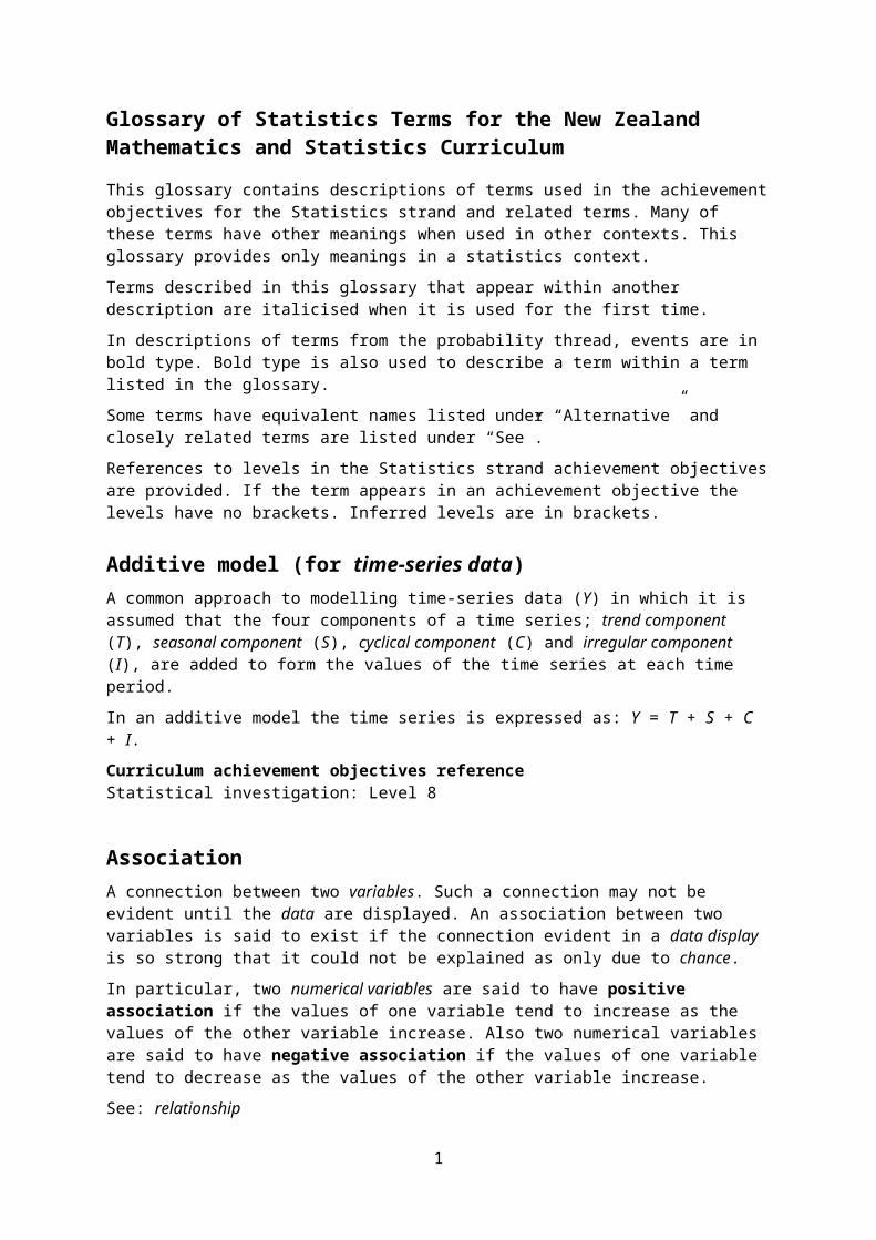
The number of days in a week that rain fell in Grey Lynn, Auckland, from Monday 2 January 2006 to Sunday 31 December 2006 is displayed on the bar graph below.

2

0 1 2 3 4 5 6 7

Rainy days per week, Auckland, 2006

Number of days with rain

Num

ber

of w

eeks

05

1015

20

Example 2

World gold mine production for 2003 by country, based on official exports, is displayed on the bar graph below.

Alternatives: bar chart, bar plot, column graph (if the bars are vertical)

Curriculum achievement objectives referencesStatistical investigation: Levels (2), (3), (4), (5), (6), (7), (8)

BiasAn influence that leads to results which are systematically less than (or greater than) the true value. For example, a biased sample is one in which the method used to create the sample would produce samples that are systematically unrepresentative of the population.

Note that random sampling can also produce an unrepresentative sample. This is not an example of bias because the random sampling process does not systematically produce unrepresentative samples and, if the process were repeated many times, the samples would balance out on average.


Binomial distributionA family of theoretical distributions that is useful as a model for some discrete random variables. Each distribution in this family gives the probability of obtaining a specified number of successes in a specified number of trials, under the following conditions:

The number of trials, n, is fixed The trials are independent of each other Each trial has two outcomes; ‘success’ and ‘failure’ The probability of success in a trial, π, is the same in each trial.

3

Sou

th A

fric

a

Aus

tral

ia

Uni

ted

Sta

tes

Chi

na

Per

u

Rus

sia

Can

ada

Indo

nesi

a

Uzb

ekis

tan

Gha

na

Pap

ua N

ew G

uine

a

Bra

zil

Col

ombi

a

Tanz

ania

Mal

i

Chi

le

Arm

enia

Res

t

Gold Production by Country, 2003G

old

prod

uctio

n (t

onne

s)

0

100

200

300

400

Each member of this family of distributions is uniquely identified by specifying n and π. As such, n and π, are the parameters of the binomial distribution and the distribution is sometimes written as binomial(n , π).

Let random variable X represent the number of successes in n trials that satisfy the conditions stated above. The probability of x successes in n trials is calculated by:

P(X = x) = for x = 0, 1, 2, ..., n

where is the number of combinations of n objects taken x at a time.

Example

A graph of the probability function for the binomial distribution with n = 6 and π = 0.4 is shown below.

Curriculum achievement objectives referenceProbability: Level 8

Bivariate dataA pair of variables from a data set with at least two variables.

Example

Consider a data set consisting of the heights, ages, genders and eye colours of a class of Year 9 students. The two variables from the data set could be:

both numerical (height and age),both category (gender and eye colour), orone numerical and one category (height and gender, respectively).

Note: Part of a Level Eight achievement objective states “including linear regression for bivariate data”. This use of bivariate data implies that both variables are numerical (i.e., quantitative variables).

Curriculum achievement objectives referencesStatistical investigation: Levels (3), (4), (5), (6), (7), 8

4

0 1 2 3 4 5 6

Pro

babi

lity

0.00

0.05

0.10

0.15

0.20

0.25

0.30

Binomial distribution (n = 6, 0.4)

Box and whisker plotA graph for displaying the distribution of a numerical variable, usually a measurement variable.

Box and whisker plots are drawn in several different forms. All of them have a ‘box’ that extends from the lower quartile to the upper quartile, with a line or other marker drawn at the median. In the simplest form, one whisker is drawn from the upper quartile to the maximum value and the other whisker is drawn from the lower quartile to the minimum value.

Box and whisker plots are particularly useful for comparing the distribution of a numerical variable for two or more categories of a category variable by displaying side-by-side box and whisker plots on the same scale. Box and whisker plots are particularly useful when the number of values to be plotted is reasonably large.

Box and whisker plots may be drawn horizontally or vertically.

Example

The actual weights of random samples of 50 male and 50 female students enrolled in an introductory Statistics course at the University of Auckland are displayed on the box and whisker plot below.

Alternatives: box and whisker diagram, box and whisker graph, box plot


Category dataData in which the values can be organised into distinct groups. These distinct groups (or categories) must be chosen so they do not overlap and so that every value belongs to one and only one group, and there should be no doubt as to which one.

The term category data is used with two different meanings. The Curriculum uses a meaning that puts no restriction on whether or not the categories have a natural ordering. This use of category data has the same meaning as qualitative data. The other meaning restricts category data to categories which do not have a natural ordering.

5

Fem

ale

Mal

e

40 60 80 100 120

Actual weights of university students

Actual weight (kg)

Gen

der

Example

The eye colours of a class of Year 9 students.

Alternative: categorical data

See: qualitative data

Curriculum achievement objectives referencesStatistical investigation: Levels 1, 2, 3, 4, (5), (6), (7), (8)

Category variableA property that may have different values for different individuals and for which these values can be organised into distinct groups. These distinct groups (or categories) must be chosen so they do not overlap and so that every value belongs to one and only one group, and there should be no doubt as to which one.

The term category variable is used with two different meanings. The Curriculum uses a meaning that puts no restriction on whether or not the categories have a natural ordering. This use of category variable has the same meaning as qualitative variable. The other meaning of category variable is restricted to categories which do not have a natural ordering.

Example


Alternative: categorical variable

See: qualitative variable

Curriculum achievement objectives referencesStatistical investigation: Levels (4), (5), (6), (7), (8)

Causal-relationship claimA statement that asserts that changes in a phenomenon (the response) are caused by differences in a received treatment or by differences in the value of another variable (an explanatory variable).

Such claims can be justified only if the observed phenomenon is a response from a well-designed and well-conducted experiment.

Curriculum achievement objectives referenceStatistical literacy: Level 8

6

Central limit theoremThe fact that the sampling distribution of the sample mean of a numerical variable becomes closer to the normal distribution as the sample size increases. The sample means are from random samples from some population.

This result applies regardless of the shape of the population distribution of the numerical variable.

The use of ‘central’ in this term is because there is a tendency for values of the sample mean to be closer to the ‘centre’ of the population distribution than individual values are. This tendency strengthens as the sample size increases.

The use of ‘limit’ in this term is because the closeness or approximation to the normal distribution improves as the sample size increases.

See: sampling distribution


Centred moving averageSee: moving mean

Curriculum achievement objectives referenceStatistical investigation: (Level 8)

ChanceA concept that applies to situations that have a number of possible outcomes, none of which is certain to occur when a trial of the situation is performed.

Two examples of situations that involve elements of chance follow.

Example 1

A person will be selected and their eye colour recorded.

Example 2

Two dice will be rolled and the numbers on each die recorded.

Curriculum achievement objectives referencesProbability: All levels

Class intervalOne of the non-overlapping intervals into which the range of values of measurement data, and occasionally whole-number data, is divided. Each value in the distribution must be able to be classified into exactly one of these intervals.

7

Example 1 (Measurement data)

The number of hours of sunshine per week in Grey Lynn, Auckland, from Monday 2 January 2006 to Sunday 31 December 2006 is recorded in the frequency table below. The class intervals used to group the values of weekly hours of sunshine are listed in the first column of the table.

Hours of sunshine Number of weeks5 to less than 10 2

10 to less than 15 215 to less than 20 520 to less than 25 925 to less than 30 1230 to less than 35 1035 to less than 40 540 to less than 45 645 to less than 50 1

Total 52

Example 2 (Whole-number data)

Students enrolled in an introductory Statistics course at the University of Auckland were asked to complete an online questionnaire. One of the questions asked them to enter the number of countries they had visited, other than New Zealand. The class intervals used to group the values are listed in the first column of the table.

Number of countries visited Frequency0 – 4 4465 – 9 172

10 – 14 6915 – 19 1920 – 24 1425 – 29 430 – 34 3Total 727

Alternatives: bin, class


8

Cleaning dataThe process of finding and correcting (or removing) errors in a data set in order to improve its quality.

Mistakes in data can arise in many ways such as:

A respondent may interpret a question in a different way from that intended by the writer of the question.

An experimenter may misread a measuring instrument.

A data entry person may mistype a value.

Curriculum achievement objectives referencesStatistical investigation: Levels 5, (6), (7), (8)

Cluster (in a distribution of a numerical variable)A distinct grouping of neighbouring values in a distribution of a numerical variable that occur noticeably more often than values on each side of these neighbouring values. If a distribution has two or more clusters then they will be separated by places where values are spread thinly or are absent.

In distributions with a small number of values or with values that are spread thinly, some values may appear to form small clusters. Such groupings may be due to natural variation (see sources of variation) and these groupings may not be apparent if the distribution had more values. Be cautious about commenting on small groupings in such distributions.

For the use of ‘cluster’ in cluster sampling see the description of cluster sampling.

Example 1

The number of hours of sunshine per week in Grey Lynn, Auckland, from Monday 2 January 2006 to Sunday 31 December 2006 is displayed in the dot plot below.

From the greater density of the dots in the plot we can see that the values have one cluster from about 23 to 37 hours per week of sunshine.

9

0 10 20 30 40 50

Sunshine hours per week, Auckland, 2006

Weekly hours of sunshine

Example 2

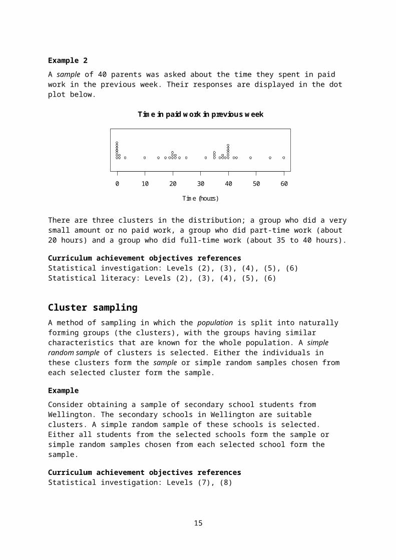
A sample of 40 parents was asked about the time they spent in paid work in the previous week. Their responses are displayed in the dot plot below.

There are three clusters in the distribution; a group who did a very small amount or no paid work, a group who did part-time work (about 20 hours) and a group who did full-time work (about 35 to 40 hours).

Curriculum achievement objectives referencesStatistical investigation: Levels (2), (3), (4), (5), (6)Statistical literacy: Levels (2), (3), (4), (5), (6)

Cluster samplingA method of sampling in which the population is split into naturally forming groups (the clusters), with the groups having similar characteristics that are known for the whole population. A simple random sample of clusters is selected. Either the individuals in these clusters form the sample or simple random samples chosen from each selected cluster form the sample.

Example

Consider obtaining a sample of secondary school students from Wellington. The secondary schools in Wellington are suitable clusters. A simple random sample of these schools is selected. Either all students from the selected schools form the sample or simple random samples chosen from each selected school form the sample.

Curriculum achievement objectives referencesStatistical investigation: Levels (7), (8)

10

0 10 20 30 40 50 60

Time in paid work in previous week

Time (hours)

Coefficient of determination (in linear regression)The proportion of the variation in the response variable that is explained by the regression model.

If there is a perfect linear relationship between the explanatory variable and the response variable there will be some variation in the values of the response variable because of the variation that exists in the values of the explanatory variable. In any real data there will be more variation in the values of the response variable than the variation that would be explained by a perfect linear relationship. The total variation in the values of the response variable can be regarded as being made up of variation explained by the linear regression model and unexplained variation. The coefficient of determination is the proportion of the explained variation relative to the total variation.

If the points are close to a straight line then the unexplained variation will be a small proportion of the total variation in the values of the response variable. This means that the closer the coefficient of determination is to 1 the stronger the linear relationship.

The coefficient of determination is also used in more advanced forms of regression, and is usually represented by R2. In linear regression, the coefficient of determination, R2, is equal to the square of the correlation coefficient, i.e., R2 = r2.

Example

The actual weights and self-perceived ideal weights of a random sample of 40 female students enrolled in an introductory Statistics course at the University of Auckland are displayed on the scatter plot below. A regression line has been drawn. The equation of the regression line is predicted y = 0.6089x + 18.661 or predicted ideal weight = 0.6089 × actual weight + 18.661

The coefficient of determination, R2 = 0.822

This means that 82.2% of the variation in the ideal weights is explained by the regression model (i.e., by the equation of the regression line).


11

50 60 70 80 90

5060

7080

90

Female ideal and actual weights

Actual weight (kg)

Idea

l wei

ght (

kg)

Combined eventAn event that consists of the occurrence of two or more events.

Two different ways of combining two events A and B are: A or B, A and B.

A or B is the event consisting of outcomes that are either in A or B or both.

A and B is the event consisting of outcomes that are common to both A and B.

Example

Suppose we have a group of men and women, and each person is a possible outcome of a probability activity. A is the event that a person is a woman and B is the event that a person is taller than 170cm.

Consider A and B. The outcomes in the combined event A and B will consist of the women who are taller than 170cm.

Consider A or B. The outcomes in the combined event A or B will consist of all of the women as well as the men taller than 170cm. An alternative description is that the combined event A or B will consist of all people taller than 170cm as well as the women who are not taller than 170cm.

Alternative: compound event, joint event


12

A or B

A B

A and B

A B

Complementary eventWith reference to a given event, the event that the given event does not occur. In other words, the complementary event to an event A is the event consisting of all of the possible outcomes that are not in event A.

There are several symbols for the complement of event A. The most common are A and A .

Example

Suppose we have a group of men and women, and each person is a possible outcome of a probability activity. If A is the event that a person is aged 30 years or more, then the complement of event A, A , consists of the people aged less than 30 years.

Curriculum achievement objectives referenceProbability: (Level 8)

Conditional eventAn event that consists of the occurrence of one event based on the knowledge that another event has already occurred.

The conditional event consisting of event A occurring, knowing that event B has already occurred, is written as A | B, and is expressed as ‘event A given event B’. Event B is considered to be the ‘condition’ in the conditional event A | B.

The probability of the conditional event A | B, .

For a justification of the above formula see the example below.

Example

Suppose we have a group of men and women, and each person is a possible outcome of the probability activity of selecting a person. A is the event that a person is a woman and B is the event that a person is taller than 170cm.

Consider A | B.

Given that B has occurred, the outcomes of interest are now restricted to those taller than 170cm.

A | B will then be the women of those taller than 170cm.

13

Complement of A

A'

A

Suppose that the genders and heights of the people were as displayed in the two-way table below.

HeightTaller than

170cmNot taller

than 170cm Total

GenderMale 68 15 83Female 28 89 117Total 96 104 200

Given that B has occurred, the outcomes of interest are the 96 people taller than 170cm.

If a person is randomly selected from these 96 people then the probability that the person is female

is, .

If both parts of the fraction are divided by 200 this becomes


Confidence intervalAn interval estimate of a population parameter. A confidence interval is therefore an interval of values, calculated from a random sample taken from the population, of which any number in the interval is a possible value for a population parameter.

The word ‘confidence’ is used in the term because the method that produces the confidence interval has a specified success rate (confidence level) for the percentage of times such intervals contain the true value of the population parameter in the long run. 95% is commonly used as the confidence level.


Confidence levelA specified percentage success rate for a method that produces a confidence interval, meaning that the method has this rate for the percentage of times such intervals contain the true value of the population parameter in the long run.

The most commonly used confidence level is 95%.


14

Confidence limitsThe lower and upper boundaries of a confidence interval.


Continuous distributionThe variation in the values of a variable that can take any value in an (appropriately-sized) interval of numbers.

A continuous distribution may be an experimental distribution, a sample distribution or a theoretical distribution of a measurement variable. Although the recorded values in an experimental or sample distribution may be rounded, the distribution is usually still regarded as being continuous.

Example

The normal distribution is an example of a theoretical continuous distribution.

Curriculum achievement objectives referencesStatistical investigation: Levels (5), (6), (7), (8)Probability: Levels (5), (6), 7, (8)

Continuous random variableA random variable that can take any value in an (appropriately-sized) interval of numbers.

Example

The height of a randomly selected individual from a population.

Curriculum achievement objectives referencesProbability: Levels (7), 8

CorrelationThe strength and direction of the relationship between two numerical variables.

In assessing the correlation between two numerical variables one variable does not need to be regarded as the explanatory variable and the other as the response variable, as is necessary in linear regression.

Two numerical variables have positive correlation if the values of one variable tend to increase as the values of the other variable increase.

Two numerical variables have negative correlation if the values of one variable tend to decrease as the values of the other variable increase.

Correlation is often measured by a correlation coefficient, the most common of which measures the strength and direction of the linear relationship between two numerical variables. In this linear case, correlation describes how close points on a scatter plot are to lying on a straight line.

15

See: correlation coefficient


Correlation coefficientA number between -1 and 1 calculated so that the number represents the strength and direction of the linear relationship between two numerical variables.

A correlation coefficient of 1 indicates a perfect linear relationship with positive slope. A correlation coefficient of -1 indicates a perfect linear relationship with negative slope.

The most widely used correlation coefficient is called Pearson’s (product-moment) correlation coefficient and it is usually represented by r.

Some other properties of the correlation coefficient, r:

1. The closer the value of r is to 1 or -1, the stronger the linear relationship.

2. r has no units.

3. r is unchanged if the axes on which the variables are plotted are reversed.

4. If the units of one, or both, of the variables are changed then r is unchanged.

Example

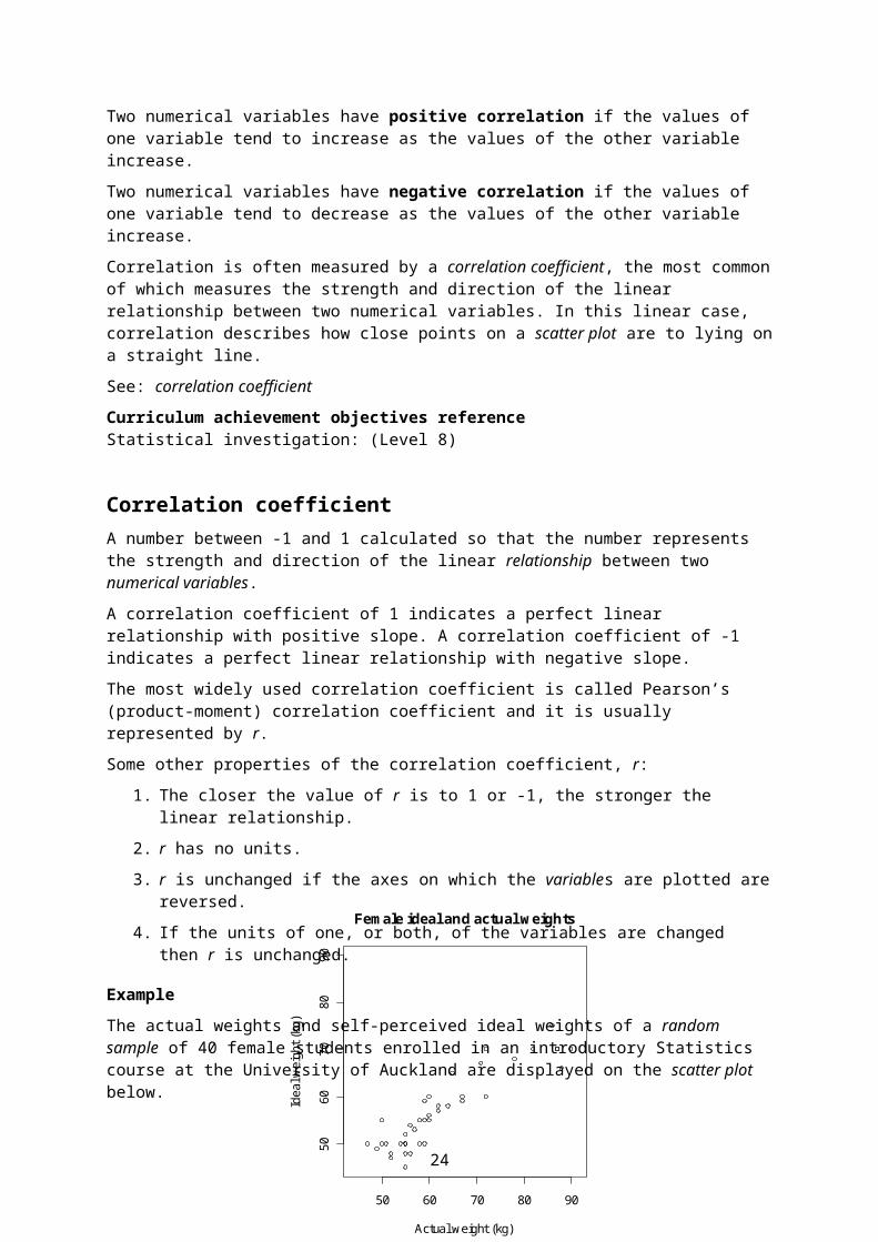
The actual weights and self-perceived ideal weights of a random sample of 40 female students enrolled in an introductory Statistics course at the University of Auckland are displayed on the scatter plot below.

The correlation coefficient, r = 0.906

See: coefficient of determination (in linear regression), correlation


16

50 60 70 80 90

5060

7080

90


Actual weight (kg)

Idea

l wei

ght (

kg)

Cyclical component (for time-series data)Long-term variations in time-series data that repeat in a reasonably systematic way over time. The cyclical component can often be represented by a wave-shaped curve, which represents alternating periods of expansion and contraction. The successive waves of the curve may have different periods.

Cyclical components are difficult to analyse and at Level Eight cyclical components can be described along with the trend.

See: time-series data


DataA term with several meanings.

Data can mean a collection of facts, numbers or information; the individual values of which are often the results of an experiment or observations.

If the data are in the form of a table with the columns consisting of variables and the rows consisting of values of each variable for different individuals or values of each variable at different times, then data has the same meaning as data set.

Data can also mean the values of one or more variables from a data set.

Data can also mean a variable or some variables from a data set.

Properly, data is the plural of datum, where a datum is any result. In everyday usage the term ‘data’ is often used in the singular.

See: data set

Curriculum achievement objectives referencesStatistical investigation: All levelsStatistical literacy: Levels 2, (3), (4), 5, (6), (7), (8)

Data displayA representation, usually as a table or graph, used to explore, summarise and communicate features of data.

Data displays listed in this glossary are: bar graph, box and whisker plot, dot plot, frequency table, histogram, line graph, one-way table, picture graph, pie graph, scatter plot, stem-and-leaf plot, strip graph, tally chart, two-way table.

Curriculum achievement objectives referencesStatistical investigation: Levels 1, 2, 3, 4, 5, 6, (7), (8)Statistical literacy: Levels 2, 3, (4), (5), 6

17

Data setA table of numbers, words or symbols; the values of which are often the results of an experiment or observations. Data sets almost always have several variables.

Usually the columns of the table consist of variables and the rows consist of values of each variable for individuals or values of each variable at different times.

Example 1 (Values for individuals)

The table below shows part of a data set resulting from answers to an online questionnaire from 727 students enrolled in an introductory Statistics course at the University of Auckland.

Individual Gender Birthmonth

Birthyear Ethnicity

Number of years living in

NZ

Number of

countries visited

Actual weight

(kg)

Ideal weight

(kg)

1 female Jan 1984 Other European 2 3 55 502 female Nov 1990 Chinese 15 11 53 493 male Jan 1990 NZ European 18 2 68 60...

.

.

.

.

.

.

.

.

.

.

.

.

.

.

.

.

.

.

.

.

.

.

.

.

Example 2 (Values at different times)

The table below shows part of a data set resulting from observations at a weather station in Rolleston, Canterbury, for each day in November 2008.

Day Max temp (°C) Rainfall (mm) Max pressure (hPa) Max wind gust (km/h)1 26.8 0.5 1015.1 70.32 19.7 0.0 1015.6 38.93 19.5 0.0 1011.1 29.6...

.

.

.

.

.

.

.

.

.

.

.

.

Alternative: dataset

Curriculum achievement objectives referencesStatistical investigation: Levels 3, (4), 5, (6), 7, 8

Dependent variableA common alternative term for the response variable in bivariate data.

Alternatives: outcome variable, output variable, response variable


18

Descriptive statisticsNumbers calculated from a data set to summarise the data set and to aid comparisons within and among variables in the data set.

Alternatives: numerical summary, summary statistics


Discrete distributionThe variation in the values of a variable that can only take on distinct values, usually whole numbers.

A discrete distribution could be an experimental distribution, a sample distribution or a theoretical distribution.

Example

The binomial distribution is an example of a theoretical discrete distribution.

Curriculum achievement objectives referencesStatistical investigation: Levels (5), (6), (7), (8)Probability: Levels 5, 6, 7, (8)

Discrete random variableA random variable that can take only distinct values, usually whole numbers.

Example

The number of left-handed people in a random selection of 10 individuals from a population is a discrete random variable. The distinct values of the random variable are 0, 1, 2, … , 10.


Discrete situationsSituations involving elements of chance in which the outcomes can take only distinct values.

If the outcomes are categories then this is a discrete situation. If the outcomes are numerical then the distinct values are often whole numbers.


19

Disjoint eventsAlternative: mutually exclusive events


DistributionThe variation in the values of a variable.

The type of distribution can be described by the type of variable (e.g., continuous distribution, discrete distribution) or by the way the values were obtained (e.g., experimental distribution, population distribution, sample distribution). Other types of distribution described in this glossary are frequency distribution, sampling distribution, theoretical distribution.

See: continuous distribution, discrete distribution, experimental distribution, frequency distribution, population distribution, sample distribution, sampling distribution, theoretical distribution

Curriculum achievement objectives referencesStatistical investigation: Levels 4, 5, 6, (7), (8)Probability: Levels 4, 5, 6, 7, 8

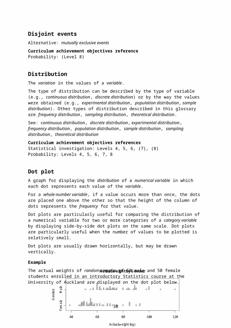
Dot plotA graph for displaying the distribution of a numerical variable in which each dot represents each value of the variable.

For a whole-number variable, if a value occurs more than once, the dots are placed one above the other so that the height of the column of dots represents the frequency for that value.

Dot plots are particularly useful for comparing the distribution of a numerical variable for two or more categories of a category variable by displaying side-by-side dot plots on the same scale. Dot plots are particularly useful when the number of values to be plotted is relatively small.

Dot plots are usually drawn horizontally, but may be drawn vertically.

Example

The actual weights of random samples of 50 male and 50 female students enrolled in an introductory Statistics course at the University of Auckland are displayed on the dot plot below.

20

40 60 80 100 120

Fem

ale

Mal

e

Actual weight by Gender

Actual weight (kg)

Gen

der

Alternative: dot graph, dotplot

Curriculum achievement objectives referencesStatistical investigation: Levels (3), (4), (5), (6), (7), (8)

EstimateA number calculated from a sample, often a random sample, which is used as an approximate value for a population parameter.

Example

A sample mean, calculated from a random sample taken from a population, is an estimate of the population mean.

Alternative: point estimate

See: interval estimate

Curriculum achievement objectives referencesStatistical investigation: Levels (6), 7, 8

EventA collection of outcomes from a probability activity or a situation involving an element of chance.

An event that consists of one outcome is called a simple event. An event that consists of more than one outcome is called a compound event.

Example 1

In a situation where a person will be selected and their eye colour recorded; blue, grey or green is an event (consisting of the 3 outcomes: blue, grey, green).

Example 2

In a situation where two dice will be rolled and the numbers on each die recorded, a total of 5 is an event (consisting of the 4 outcomes: (1, 4), (2, 3), (3, 2), (4, 1), where (1, 4) means a 1 on the first die and a 4 on the second).

Example 3

In a situation where a person will be selected at random from a population and their weight recorded, heavier than 70kg is an event.

Curriculum achievement objectives referencesProbability: Levels (5), (6), (7), 8

Expected value (of a discrete random variable)The population mean for a random variable and is therefore a measure of centre for the distribution of a random variable.

The expected value of random variable X is often written as E(X) or µ or µX.

21

The expected value is the ‘long-run mean’ in the sense that, if as more and more values of the random variable were collected (by sampling or by repeated trials of a probability activity), the sample mean becomes closer to the expected value.

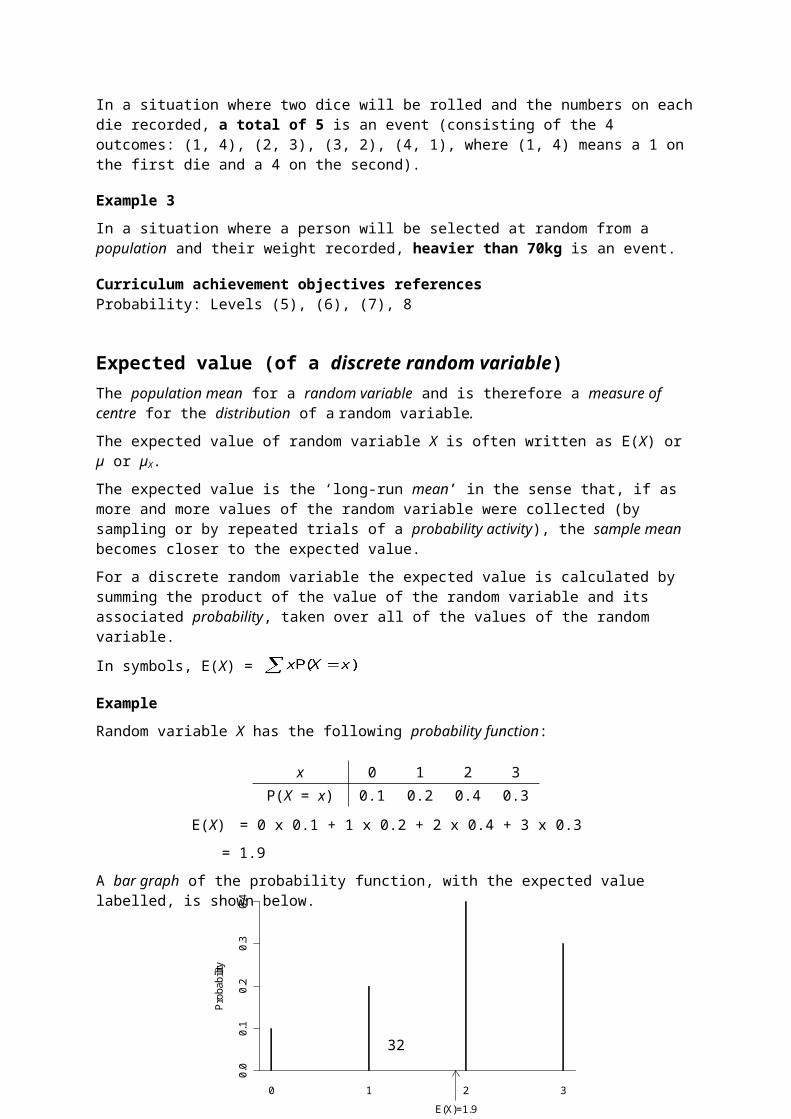
For a discrete random variable the expected value is calculated by summing the product of the value of the random variable and its associated probability, taken over all of the values of the random variable.

In symbols, E(X) =

Example

Random variable X has the following probability function:

x 0 1 2 3P(X = x) 0.1 0.2 0.4 0.3

E(X) = 0 x 0.1 + 1 x 0.2 + 2 x 0.4 + 3 x 0.3

= 1.9

A bar graph of the probability function, with the expected value labelled, is shown below.

See: population mean


ExperimentIn its simplest meaning, a process or study that results in the collection of data, the outcome of which is unknown.

In the statistical literacy thread at Level Eight, experiment has a more specific meaning. Here an experiment is a study in which a researcher attempts to understand the effect that a variable (an explanatory variable) may have on some phenomenon (the response) by controlling the conditions of the study.

In an experiment the researcher controls the conditions by allocating individuals to groups and allocating the value of the explanatory variable to be received by each group. A value of the explanatory variable is called a treatment.

22

0 1 2 3

Pro

babi

lity

0.0

0.1

0.2

0.3

0.4

E(X)=1.9

In a well-designed experiment the allocation of subjects to groups is done using randomisation. Randomisation attempts to make the characteristics of each group very similar to each other so that if each group was given the same treatment the groups should respond in a similar way, on average.

Experiments usually have a control group, a group that receives no treatment or receives an existing or established treatment. This allows any differences in the response, on average, between the control group and the other group(s) to be visible.

When the groups are similar in all ways apart from the treatment received, then any observed differences in the response (if large enough) among the groups, on average, is said to be caused by the treatment.

Example

In the 1980s the Physicians’ Health Study investigated whether a low dose of aspirin had an effect on the risk of a first heart attack for males. The study participants, about 22,000 healthy male physicians from the United States, were randomly allocated to receive aspirin or a placebo. About 11,000 were allocated to each group.

This is an experiment because the researchers allocated individuals to two groups and decided that one group would receive a low dose of aspirin and the other group would receive a placebo. The treatments are aspirin and placebo. The response was whether or not the individual had a heart attack during the study period of about five years.

See: causal-relationship claim, placebo, randomisation

Curriculum achievement objectives referencesStatistical investigation: Levels 5, (6), 7, 8Statistical literacy: Level 8

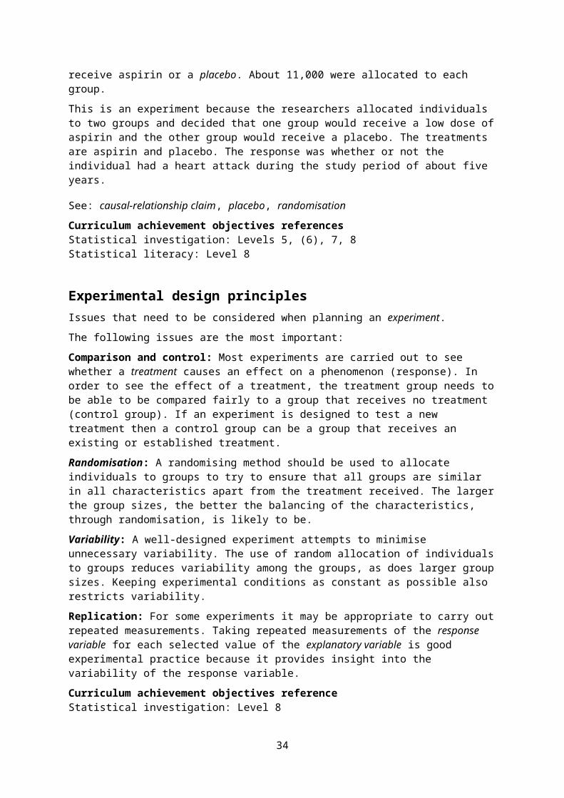
Experimental design principlesIssues that need to be considered when planning an experiment.

The following issues are the most important:

Comparison and control: Most experiments are carried out to see whether a treatment causes an effect on a phenomenon (response). In order to see the effect of a treatment, the treatment group needs to be able to be compared fairly to a group that receives no treatment (control group). If an experiment is designed to test a new treatment then a control group can be a group that receives an existing or established treatment.

Randomisation: A randomising method should be used to allocate individuals to groups to try to ensure that all groups are similar in all characteristics apart from the treatment received. The larger the group sizes, the better the balancing of the characteristics, through randomisation, is likely to be.

Variability: A well-designed experiment attempts to minimise unnecessary variability. The use of random allocation of individuals to groups reduces variability among the groups, as does larger group sizes. Keeping experimental conditions as constant as possible also restricts variability.

Replication: For some experiments it may be appropriate to carry out repeated measurements. Taking repeated measurements of the response variable for each selected value of the explanatory variable is good experimental practice because it provides insight into the variability of the response variable.

23


Experimental distributionThe variation in the values of a variable obtained from the results of carrying out trials of a situation that involves elements of chance, a probability activity, or a statistical experiment.

For whole-number data, an experimental distribution is often displayed, in a table, as a set of values and their corresponding frequencies, or on an appropriate graph.

For measurement data, an experimental distribution is often displayed, in a table, as a set of intervals of values (class intervals) and their corresponding frequencies, or on an appropriate graph.

For category data, an experimental distribution is often displayed, in a table, as a set of categories and their corresponding frequencies, or on an appropriate graph.

Alternative: empirical distribution

See: sample distribution

Curriculum achievement objectives referencesProbability: Levels 4, 5, 6, 7

Explanatory variableThe variable, of the two variables in bivariate data, knowledge of which may provide information about the other variable, the response variable. Knowledge of the explanatory variable may be used to predict values of the response variable, or changes in the explanatory variable may be used to predict how the response variable will change.

If the bivariate data result from an experiment then the explanatory variable is the one whose values can be manipulated or selected by the experimenter.

In a scatter plot, as part of a linear regression analysis, the explanatory variable is placed on the x-axis (horizontal axis).

Alternatives: independent variable, input variable, predictor variable


Exploratory data analysisThe process of identifying patterns and features within a data set by using a wide range of graphs and summary statistics. Exploratory data analysis usually starts with graphs and summary statistics of single variables and then extends to pairs of variables and further combinations of variables.

Exploratory data analysis is an essential part of the statistical enquiry cycle. It is important at the cleaning data stage because graphs may reveal data that need checking with regard to quality of the data set.

For data sets about populations exploratory data analysis will reveal important features of the population, and for data sets from samples it will reveal features of the sample which may suggest features in the population from which the sample was taken.

24

For bivariate numerical data exploratory data analysis will indicate whether it is appropriate to fit a linear regression model to the data.

For time-series data exploratory data analysis will indicate whether it is appropriate to fit an additive model to the time-series data.

Curriculum achievement objectives referencesStatistical investigation: Levels (1), (2), (3), (4), (5), (6), 7, 8

ExtrapolationThe process of estimating the value of one variable based on knowing the value of the other variable, where the known value is outside the range of values of that variable for the data on which the estimation is based.

Curriculum achievement objectives referencesStatistical investigation: Levels 7, (8)

Features (of distributions)Distinctive parts of distributions which usually become apparent when the distribution is presented in a data display. The parts worthy of comment will depend on the type of display and how clearly the part stands out.

Curriculum achievement objectives referencesStatistical investigation: Levels (2), (3), (4), (5), 6, (7), (8)Statistical literacy: Levels 2, (3), (4), (5), (6), (7), (8)

Five-number summaryFive numbers that form a summary for the distribution of a numerical variable. The five numbers are: minimum value, lower quartile, median, upper quartile, maximum value. Together they convey quite a lot of information about the features of the distribution.

Example

The five-number summary for the weights of the 302 male students who answered an online questionnaire given to students enrolled in an introductory Statistics course at the University of Auckland is 51kg, 65kg, 72kg, 81kg, 140kg.


ForecastAn assessment of the value of a variable at some future point of time, often based on an analysis of time-series data.


25

FrequencyFor a whole-number variable in a data set, the number of times a value occurs.

For a measurement variable in a data set, the number of occurrences in a class interval.

For a category variable in a data set, the number of occurrences in a category.

See: relative frequency, tally chart


Frequency distributionFor whole-number data, a set of values and their corresponding frequencies displayed in a table, or the set of values displayed on an appropriate graph.

For measurement data, a set of intervals of values (class intervals) and their corresponding frequencies displayed in a table, or the set of values displayed on an appropriate graph.

For category data, a set of categories and their corresponding frequencies displayed in a table or graph.

See: experimental distribution, frequency table, sample distribution

Curriculum achievement objectives referencesStatistical investigation: Levels (4), (5), (6), (7), (8)Probability: Levels (4), (5), (6), (7), (8)

Frequency tableAny table that displays the frequencies of values of one or more variables in a data set.

For a whole-number variable in a data set, a table showing each value of the variable and its corresponding frequency.

For a measurement variable in a data set, a table showing a set of class intervals for the variable and the corresponding frequency for each interval.

For a category variable in a data set, a table showing each category of the variable and its corresponding frequency.

A frequency table will often have an extra column that shows the percentages that fall in each value, class interval or category.

See: one-way table, two-way table

26

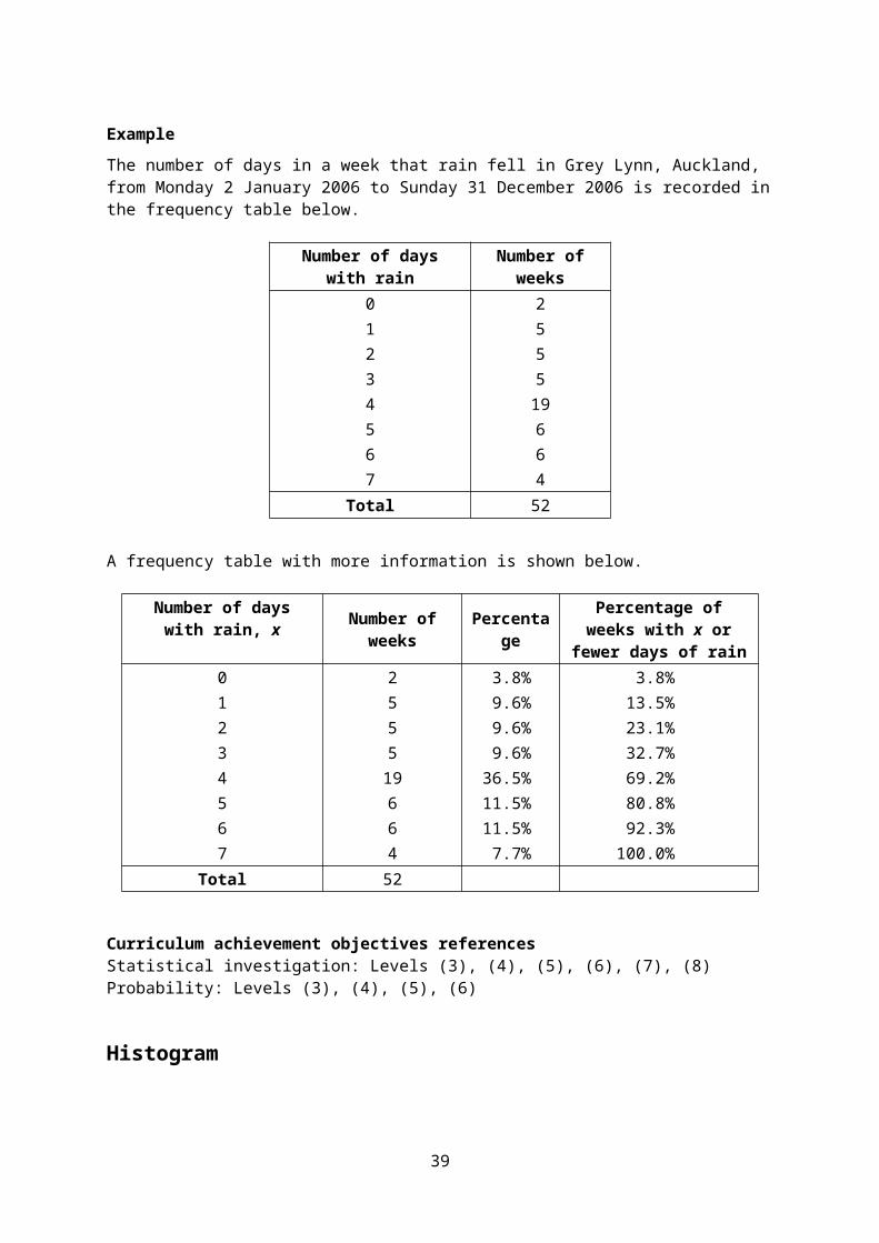
Example

The number of days in a week that rain fell in Grey Lynn, Auckland, from Monday 2 January 2006 to Sunday 31 December 2006 is recorded in the frequency table below.

Number of days with rain Number of weeks0 21 52 53 54 195 66 67 4

Total 52

A frequency table with more information is shown below.

Number of days with rain, x Number of weeks Percentage Percentage of weeks with

x or fewer days of rain0 2 3.8% 3.8%1 5 9.6% 13.5%2 5 9.6% 23.1%3 5 9.6% 32.7%4 19 36.5% 69.2%5 6 11.5% 80.8%6 6 11.5% 92.3%7 4 7.7% 100.0%

Total 52

Curriculum achievement objectives referencesStatistical investigation: Levels (3), (4), (5), (6), (7), (8)Probability: Levels (3), (4), (5), (6)

HistogramA graph for displaying the distribution of a measurement variable consisting of vertical rectangles, drawn for each class interval, whose area represents the relative frequency for values in that class interval.

To aid interpretation, it is desirable to have equal-width class intervals so that the height of each rectangle represents the frequency (or relative frequency) for values in each class interval.

Histograms are particularly useful when the number of values to be plotted is large.

27

Example

The number of hours of sunshine per week in Grey Lynn, Auckland, from Monday 2 January 2006 to Sunday 31 December 2006 is displayed in the histogram below.


Independence (in situations that involve elements of chance)The property that an outcome of one trial of a situation involving elements of chance or a probability activity has no effect or influence on an outcome of any other trial of that situation or activity.

Curriculum achievement objectives referencesProbability: Levels 4, (5), (6), (7), (8)

Independent eventsEvents that have no influence on each other.

Two events are independent if the fact that one of the events has occurred has no influence on the probability of the other event occurring.

If events A and B are independent then:

P(A | B) = P(A)

P(B | A) = P(B)

P(A and B) = P(A) P(B), where P(E) represents the probability of event E occurring.

For two events A and B:

If P(A | B)= P(A) then A and B are independent events

If P(B | A)= P(B) then A and B are independent events

If P(A and B) = P(A) P(B) then A and B are independent events.

28



Num

ber

of w

eeks

5 10 15 20 25 30 35 40 45 50

04

812


Independent variableA common alternative term for the explanatory variable in bivariate data.

Alternatives: explanatory variable, input variable, predictor variable


Index numberA number showing the size of a quantity relative to its size at a chosen period, called the base period.

The price index for a certain ‘basket’ of shares, goods or services aims to show how the price has changed while the quantities in the basket remain fixed. The index at the base period is a convenient number such as 100 (or 1000). An index greater than 100 (or 1000) at a later time period indicates that the basket has increased in value or price relative to that at the base period.


InferenceSee: statistical inference

Curriculum achievement objectives referencesStatistical investigation: Levels 6, 7, 8

InterpolationThe process of estimating the value of one variable based on knowing the value of the other variable, where the known value is within the range of values of that variable for the data on which the estimation is based.


Interquartile rangeA measure of spread for a distribution of a numerical variable which is the width of an interval that contains the middle 50% (approximately) of the values in the distribution. It is calculated as the difference between the upper quartile and lower quartile of a distribution.

It is recommended that, for small data sets, this measure of spread is calculated by sorting the values into order or displaying them on a suitable plot and then counting values to find the quartiles, and to use software for large data sets.

29

The interquartile range is a stable measure of spread in that it is not influenced by unusually large or unusually small values. The interquartile range is more useful as a measure of spread than the range because of this stability. It is recommended that a graph of the distribution is used to check the appropriateness of the interquartile range as a measure of spread and to emphasise its meaning as a feature of the distribution.

Example

The maximum temperatures, in degrees Celsius (°C), in Rolleston for the first 10 days in November 2008 were: 18.6, 19.9, 20.6, 19.4, 17.8, 18.1, 17.8, 18.7, 19.6, 18.8

Ordered values: 17.8, 17.8, 18.1, 18.6, 18.7, 18.8, 19.4, 19.6, 19.9, 20.6

The median is the mean of the two central values, 18.7 and 18.8. Median = 18.75°C

The values in the ‘lower half’ are 17.8, 17.8, 18.1, 18.6, 18.7. Their median is 18.1. The lower quartile is 18.1°C.

The values in the ‘upper half’ are 18.8, 19.4, 19.6, 19.9, 20.6. Their median is 19.6. The upper quartile is 19.6°C.

The interquartile range is 19.6°C – 18.1°C = 1.5°C

The data and the interquartile range are displayed on the dot plot below.

See: lower quartile, measure of spread, quartiles, upper quartile


Interval estimateA range of numbers, calculated from a random sample taken from the population, of which any number in the range is a possible value for a population parameter.

Example

A 95% confidence interval for a population mean is an interval estimate.

See: estimate


30

17 18 19 20 21

Maximum temperatures, Rolleston

Temperature (degrees Celsius)

l.q. median u.q.

interquartile range

InvestigationSee: statistical investigation

Curriculum achievement objectives referencesStatistical investigation: All levelsStatistical literacy: Levels 1, 2, 3, 4, 5

Irregular component (for time-series data)The other variations in time-series data that are not identified as part of the trend component, cyclical component or seasonal component. They mostly consist of variations that don’t have a clear pattern.

Alternative: random error component



Least-squares regression lineThe most common method of choosing the line that best summarises the linear relationship (or linear trend) between the two variables in a linear regression analysis, from the bivariate data collected.

Of the many lines that could usefully summarise the linear relationship, the least-squares regression line is the one line with the smallest sum of the squares of the residuals.

Two other properties of the least-squares regression line are:

1. The sum of the residuals is zero.

2. The point with x-coordinate equal to the mean of the x-coordinates of the observations and with y-coordinate equal to the mean of the y-coordinates of the observations is always on the least-squares regression line.


LikelihoodThe notion of an outcome being probable. Likelihood is sometimes used as a simpler alternative to probability.

In a situation involving elements of chance, equal likelihoods mean that, for any trial, each outcome has the same chance of occurring.

Similarly, different likelihoods mean that, for any trial, not all of the outcomes have the same chance of occurring.


31

Line graphA graph, often used for displaying time-series data, in which a series of points representing individual observations are connected by line segments.

Line graphs are useful for showing changes in a variable over time.

Example

Daily sales, in thousands of dollars, for a hardware store were recorded for 28 days. These data are displayed on the line graph below.


Linear regressionA form of statistical analysis that uses bivariate data (where both are numerical variables) to examine how knowledge of one of the variables (the explanatory variable) provides information about the values of the other variable (the response variable). The roles of the explanatory and response variables are therefore different.

When the bivariate numerical data are displayed on a scatter plot, the relationship between the two variables becomes visible. Linear regression fits a straight line to the data that is added to the scatter plot. The fitted line helps to show whether or not a linear regression model is a good fit to the data.

If a linear regression model is appropriate then the fitted line (regression line) is used to predict a value of the response variable for a given value of the explanatory variable and to describe how the values of the response variable change, on average, as the values of the explanatory variable change.

An appropriately fitted linear regression model estimates the true, but unknown, linear relationship between the two variables and the underlying system the data was taken from is regarded as having two components: trend (the general linear tendency) and scatter (variation from the trend).

32

0

50

100

150

200

250

300

Shop sales

Day

Sal

es, t

hous

ands

of d

olla

rs

M Tu W Th F Sa Su M Tu W Th F Sa Su M Tu W Th F Sa Su M Tu W Th F Sa Su

Note: Linear regression can be used when there is more than one explanatory variable, but at Level Eight only one explanatory variable is used. When there is one explanatory variable the method is called simple linear regression.


Lower quartileSee: quartiles


Margin of errorA number calculated from a random sample that estimates the likely size of the sampling error in an estimate of a population parameter.

The margin of error is added to and subtracted from a point estimate of a population parameter to form a confidence interval for a population parameter, usually with a confidence level of 95%. The margin of error is therefore half of the width of a confidence interval.

Generally a larger sample size will give a smaller margin of error.

The higher the confidence level, the greater the margin of error.

Curriculum achievement objectives referencesStatistical investigation: Level 8Statistical literacy: Level 8

MeanA measure of centre for a distribution of a numerical variable. The mean is the centre of mass of the values in a distribution and is calculated by adding the values and then dividing this total by the number of values.

For large data sets it is recommended that a calculator or software is used to calculate the mean.

The mean can be influenced by unusually large or unusually small values. It is recommended that a graph of the distribution is used to check the appropriateness of the mean as a measure of centre and to emphasise its meaning as a feature of the distribution.

33

pointestimate

lowerconfidence

limit

upperconfidence

limit

of error of errormargin margin

Example


The mean maximum temperature over these 10 days is 18.93°C.

The data and the mean are displayed on the dot plot below.

Alternative: arithmetic mean

See: measure of centre, population mean, sample mean

Curriculum achievement objectives referencesStatistical investigation: Levels 5, (6), (7), 8

MeasureAn amount or quantity that is determined by measurement or calculation. The term ‘measure’ is used in two different ways in the Curriculum.

One use is in the terms; measure of centre, measure of spread and measure of proportion, where these measures are calculated quantities that represent characteristics of a distribution. The use of “using displays and measures” in the Level Six (statistical investigation thread) achievement objective is a reference to measures of centre, spread and proportion.

The other use applies to a statistical investigation. The investigator decides on a subject of interest and then decides the aspects of it that can be observed. These aspects are the ‘measures’.

Example

An investigator decides that ‘well-being’ is a subject of interest and chooses ‘happiness’ to be one aspect of well-being. Happiness could be measured by the variable ‘number of times a person laughs in a day, on average’.

Curriculum achievement objectives referencesStatistical investigation: Levels 5, 6, 7, (8)Statistical literacy: Levels 5, (6), (7), (8)

34

17 18 19 20 21



mean

Measure of centreA number that is representative or typical of the middle of a distribution of a numerical variable. The measures of centre that are used most often are the mean and the median. The mode is sometimes used.

Alternatives: measure of centrality, measure of central tendency, measure of location

See: average


Measure of proportionA sample proportion used to make comparisons among sample distributions.

Example

An online questionnaire was completed by 727 students enrolled in an introductory Statistics course at the University of Auckland. It included questions on their actual weight, gender and ethnicity.

The measurement variable ‘actual weight’ was recategorised with one category for actual weights less than 60kg. It was concluded that 56.7% of the females weighed less than 60kg compared to 7.6% of the males. This is an example of bivariate data with one measurement variable (actual weight) and one category variable (gender).

As part of a comparison between the ethnicity sample distributions for females and males it was concluded that 5.4% of the females were Korean compared to 10.9% of the males. This is an example of bivariate data with two category variables.


Measure of spreadA number that conveys the degree to which values in a distribution of a numerical variable differ from each other. The measures of spread that are used most often are: interquartile range, range, standard deviation, variance.

Alternatives: measure of variability, measure of dispersion


Measurement dataData in which the values result from measuring, meaning that the values may take on any value within an interval of numbers.

Example

The heights of a class of Year 9 students.

35

See: numerical data, quantitative data

Curriculum achievement objectives referencesStatistical investigation: Level 4, (5), (6), (7), (8)

Measurement variableA property that may have different values for different individuals and for which these values result from measuring, meaning that the values may take on any value within an interval of numbers.

Example

The heights of a class of Year 9 students.

See: numerical variable, quantitative variable


MedianA measure of centre that marks the middle of a distribution of a numerical variable.

It is recommended that, for small data sets, this measure of centre is calculated by sorting the values into order and then counting the values, and to use software for large data sets.

The median is a stable measure of centre in that it is not influenced by unusually large or unusually small values. It is recommended that a graph of the distribution is used to emphasise its meaning as a feature of the distribution.

Example 1 (Odd number of values)

The maximum temperatures, in degrees Celsius (°C), in Rolleston for the first 9 days in November 2008 were: 18.6, 19.9, 20.6, 19.4, 17.8, 18.1, 17.8, 18.7, 19.6

Ordered values: 17.8, 17.8, 18.1, 18.6, 18.7, 19.4, 19.6, 19.9, 20.6

The data and the median are displayed on the dot plot below.

The median maximum temperature over these 9 days is 18.7°C. There are 4 values below 18.7°C and 4 values above it.

36

17 18 19 20 21



median

Example 2 (Even number of values)


Ordered values: 17.8, 17.8, 18.1, 18.6, 18.7, 18.8, 19.4, 19.6, 19.9, 20.6

The mean of the two central values, 18.7 and 18.8, is 18.75.

The data and the median are displayed on the dot plot below.

The median maximum temperature over these 10 days is 18.75°C. There are 5 values below 18.75°C and 5 values above it.

Note: The median can be calculated directly from the dot plot or from the ordered values.

See: measure of centre


Modal intervalAn interval of neighbouring values for a measurement variable that occur noticeably more often than the values on each side of this interval.

37

17 18 19 20 21



median

Example

The number of hours of sunshine per week in Grey Lynn, Auckland, from Monday 2 January 2006 to Sunday 31 December 2006 is displayed in the histogram below.

The distribution has a modal interval of 25 to 30 hours of sunshine per week.


ModalityA measure of the number of modes in a distribution of a numerical variable.

A unimodal distribution has one mode, meaning that the distribution has one value (or interval of neighbouring values) that occurs noticeably more often than any other value (or values on each side of the modal interval).

A bimodal distribution has two modes, meaning that the distribution has two values (or intervals of neighbouring values) that occur noticeably more often than the values on each side of the modes (or modal intervals).

In frequency distributions of a numerical variable the word ‘cluster’ is often used to describe groups of neighbouring values that form modes or modal intervals.

38



Num

ber

of w

eeks

5 10 15 20 25 30 35 40 45 50

04

812

Example 1 (Frequency distribution, whole-number variable)

The number of days in a week that rain fell in Grey Lynn, Auckland, from Monday 2 January 2006 to Sunday 31 December 2006 is recorded in the frequency table and displayed in the bar graph below.

Number of days with rain Number of weeks

0 21 52 53 54 195 66 67 4

Total 52

This distribution is unimodal with a mode at 4 days of rain per week.

Example 2 (Theoretical distribution, continuous random variable)

The graph displays the probability density function of a theoretical distribution. It has modes at 40 and 70.

Curriculum achievement objectives referencesStatistical investigation: Levels (6), (7), (8)

ModeA value in a distribution of a numerical variable that occurs more frequently than other values.

As a measure of centre the mode is less useful than the mean or median because some distributions have more than one mode and other distributions, where no values are repeated, have no mode.

It is recommended that a graph of the distribution is used to check the appropriateness of the mode as a measure of centre and to emphasise its meaning as a feature of the distribution.

39

0 1 2 3 4 5 6 7


Number of days with rain

Num

ber

of w

eeks

05

1015

20

Bimodal theoretical distribution

0 20 40 60 80 100

Example

The number of days in a week that rain fell in Grey Lynn, Auckland, from Monday 2 January 2006 to Sunday 31 December 2006 is recorded in the frequency table and displayed on the bar graph below.


Total 52

The mode is 4 days with rain per week.


ModelA simplified or idealised description of a situation. The term model is used in two different ways in the Curriculum.

In the probability thread the use of “models of all the outcomes” refers to a list of all possible outcomes of a situation involving elements of chance and, at more advanced levels, a list of all possible outcomes and the corresponding probabilities for each outcome.

At Level Eight in the statistical investigation thread, an achievement objective refers to “appropriate models (including linear regression for bivariate data and additive models for time-series data)”. Used in this way, a model is an idealised description of the underlying system the data was taken from and the model is intended to match the data closely.

See: probability function (for a discrete random variable)

Curriculum achievement objectives referencesStatistical investigation: Level 8Probability: Levels 3, 4, (5), (6), (7), (8)

Moving averageA method used to smooth time-series data. It forms a new smoothed series in which the irregular component is reduced.

If the time series has a seasonal component a moving average is used to eliminate the seasonal component.

40

0 1 2 3 4 5 6 7


Number of days with rainN

umbe

r of

wee

ks

05

1015

20

Each value in the time series is replaced by an average of the value and a number of neighbouring values. The number of values used to calculate a moving average depends on the type of time-series data. For weekly data, seven values are used; for monthly data, 12 values are used; and for quarterly data, four values are used. If the number of values used is even, the moving average must be centred by taking a two-term moving average of the new series.

In terms of an additive model for time-series data, Y = T + S + C + I, where T represents the trend component, S represents the seasonal component, C represents the cyclical component, and I represents the irregular component;

the smoothed series = T + C.

See: centred moving average, moving mean


Moving meanA specified moving average method used to smooth time-series data. It forms a new smoothed series in which the irregular component is reduced.

If the time series has a seasonal component a moving mean may be used to eliminate the seasonal component.

Each value in the time series is replaced by the mean of the value and a number of neighbouring values. The number of values used to calculate a moving mean depends on the type of time-series data. For weekly data, seven values are used; for monthly data, 12 values are used; and for quarterly data, four values are used. If the number of values used is even, the moving mean must be centred by taking two-term moving means of each pair of consecutive moving means, forming a series of centred moving means. See Example 2 for an illustration of this technique.


the smoothed series = T + C.

41

Example 1 (Weekly data)

Daily sales, in thousands of dollars, for a hardware store were recorded for 21 days. There is reasonably systematic variation over each 7-day period and so moving means of order 7 have been calculated to attempt to eliminate this seasonal component. The moving mean for the first Thursday

is calculated by =148.14

Day Sales Moving mean($000) ($000)

Mon 86Tue 125Wed 115Thu 150 148.14Fri 168 147.71Sat 291 146.71Sun 102 146.29Mon 83 145.00Tue 118 145.43Wed 112 144.14Thu 141 143.71Fri 171 143.57Sat 282 143.43Sun 99 142.86Mon 82 144.86Tue 117 144.00Wed 108 142.43Thu 155 140.86Fri 165Sat 271Sun 88

The raw data and the moving means are displayed below.

42

50

100

150

200

250

300

Shop sales

Day

Sal

es, t

hous

ands

of d

olla

rs

M Tu W Th F Sa Su M Tu W Th F Sa Su M Tu W Th F Sa Su

salesmoving means

Example 2 (Quarterly data)

Statistics New Zealand’s Economic Survey of Manufacturing provided the following data on actual operating income for the manufacturing sector in New Zealand. There is reasonably systematic variation over each 4-quarter period and so moving means of order 4 have been calculated to attempt to eliminate this seasonal component. However these moving means do not align with the quarters; the moving means are not centred. To align the moving means with the quarters, each pair of moving means is averaged to form centred moving means.

The first moving mean (between Mar-05 and Dec-05) is calculated by

= 17531

The centred moving mean for Sep-05 is calculated by = 17548.25

Operating Moving CentredQuarter income mean moving mean

($millions) ($millions) ($millions)Mar-05 17322

Jun-05 1769617531.00

Sep-05 17060 17548.25017565.50

Dec-05 18046 17732.75017900.00

Mar-06 17460 18048.12518196.25

Jun-06 19034 18298.75018401.25

Sep-06 18245 18490.50018579.75

Dec-06 18866 18633.50018687.25

Mar-07 18174 18735.75018784.25

Jun-07 19464 19003.00019221.75

Sep-07 18633

Dec-07 20616

43

The raw data and the centred moving means are displayed below. Note that M, J, S and D indicate quarter years ending in March, June, September and December respectively.

See: moving average


Multivariate dataA data set that has several variables.

Example

A data set consisting of the heights, ages, genders and eye colours of a class of Year 9 students.

Curriculum achievement objectives referencesStatistical investigation: Levels 3, 4, 5, (6), (7), (8)

Mutually exclusive eventsEvents that cannot occur together.

If events A and B are mutually exclusive then the combined event A and B contains no outcomes.

44

16

17

18

19

20

21

Operating income, NZ manufacturing sector

Quarter

Ope

ratin

g in

com

e ($

billio

ns)

M-0

5

J-05

S-0

5

D-0

5

M-0

6

J-06

S-0

6

D-0

6

M-0

7

J-07

S-0

7

D-0

7

operating incomecentred moving means

Mutually exclusive events

A B

Example 1

Suppose we have a group of men and women, each of whom is a possible outcome of a probability activity. If A is the event that a person is aged less than 30 years and B is the event that a person is aged over 50.

The event A and B contains no outcomes because none of the people can be aged less than 30 years and over 50. Events A and B are therefore mutually exclusive.

Example 2

Consider rolling two dice. Suppose that event C consists of outcomes which have a total of 8 and that event D consists of outcomes which has the first die showing a 1.

First explanation: If the first die shows a 1 (event D has occurred) then the greatest total for the two dice is 1 + 6 = 7, meaning that a total of 8 cannot occur. In other words, event C cannot occur together with event D.

Second explanation: C consists of the outcomes (2, 6), (3, 5), (4, 4), (5, 3), (6, 2), where (2, 6) means a 2 on the first die and a 6 on the second. D consists of the outcomes (1, 1), (1, 2), (1, 3), (1, 4), (1, 5), (1, 6). No outcomes are common to both event C and event D.

Events C and D are therefore mutually exclusive.

Alternative: disjoint events


Non-sampling errorOne of the two reasons for the difference between an estimate (from a sample) and the true value of a population parameter; the other reason being the error caused because data are collected from a sample rather than the whole population (sampling error). Non-sampling errors have the potential to cause bias in surveys or samples.

There are many different types of non-sampling errors and the names used for each of them are not consistent.

Some examples of non-sampling errors are:

The sampling process is such that a specific group is excluded or under-represented in the sample, deliberately or inadvertently. If the excluded or under-represented group is different, with respect to survey issues, then bias will occur.

The sampling process allows individuals to select themselves. Individuals with strong opinions about the survey issues or those with substantial knowledge will tend to be over-represented, creating bias.

If people who refuse to answer are different, with respect to survey issues, from those who respond then bias will occur. This can also happen with people who are never contacted and people who have yet to make up their mind.

If the response rate (the proportion of the sample that takes part in a survey) is low, bias can occur because respondents may tend consistently to have views that are more extreme than those of the population in general.

45

The wording of questions, the order in which they are asked and the number and type of options offered can influence survey results.

Answers given by respondents do not always reflect their true beliefs because they may feel under social pressure not to give an unpopular or socially undesirable answer.

Answers given by respondents may be influenced by the desire to impress an interviewer.

Curriculum achievement objectives referencesStatistical investigation: Levels (7), (8)Statistical literacy: Levels 7, (8)

Normal distributionA family of theoretical distributions that is useful as a model for some continuous random variables.

Each member of this family of distributions is uniquely identified by specifying the mean µ and standard deviation σ (or variance σ2). As such, µ and σ (or σ2), are the parameters of the normal distribution, and the distribution is sometimes written as Normal(µ, σ) or Normal(µ, σ2).

The probability density function of a normal distribution is a symmetrical, bell-shaped curve, centred at its mean µ. The graphs of the probability density functions of two normal distributions are shown below, one with µ = 50 and σ = 15 and the other with µ = 50 and σ = 10.

Curriculum achievement objectives referencesProbability: Levels 7, 8

Numerical dataData in which the values result from counting or measuring. Measurement data are numerical, as are whole-number data.

Alternative: quantitative data

See: measurement data, whole-number data

Curriculum achievement objectives referencesStatistical investigation: Levels 2, 3, (4), (5), (6), (7), (8)

46

Two normal distributions

10 30 50 70 90

Normal(Normal(

=50, =50,

=10)=15)

Numerical variableA property that may have different values for different individuals and for which these values result from counting or measuring. Measurement variables are numerical, as are whole-number variables.

Alternative: quantitative variables

See: measurement variable, whole-number variable


Observational studyA study in which a researcher attempts to understand the effect that a variable (an explanatory variable) may have on some phenomenon (the response), but the researcher is not able to control some important conditions of the study.

In an observational study the researcher has no control over the value of the explanatory variable; the researcher can only observe the value of the explanatory variable for each individual and, if necessary, allocate individuals to groups based on the observed values.

Because the groups in the study are formed by values of an explanatory variable that individuals happened to receive, and not by randomisation, the groups may not be similar in all ways apart from the value of the explanatory variable.

Any observed differences in the response (if large enough) between the groups, on average, cannot be said to be caused by any differences in the values of the explanatory variable. The differences in the response could be due to the differences in the groups that are not related to the explanatory variable.

Example

A study by researchers at Harvard School of Public Health, published in 2009, investigated the relationship between low childhood IQ and adult mental health disorders. The study participants were a group of children born in 1972 and 1973 in Dunedin. Their IQs were assessed at ages 7, 9 and 11 and mental health disorders were assessed at ages 18 through to 32 in interviews by health professionals who had no knowledge of the individuals’ IQ or mental health history.

This is an observational study because the researchers had no control over the explanatory variable, childhood IQ. The researchers could only record the assessed childhood IQ. The response was whether or not the individual had suffered from a mental disorder during adulthood.

Curriculum achievement objectives referenceStatistical literacy: Level 8

47

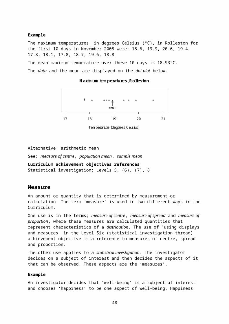
One-way tableA table for displaying category data for one variable in a data set that displays each category and its associated frequency or relative frequency.

Example

Students enrolled in an introductory Statistics course at the University of Auckland were asked to complete an online questionnaire. One of the questions asked them to enter their ethnicity. They chose from the following list: Chinese, Indian, Korean, Maori, New Zealand European, Other European, Pacific, Other. The 727 responses are displayed on the one-way table below.

Ethnicity Chinese Indian Korean Maori NZ European

Other European Pacific Other Total

Frequency 169 58 56 18 253 45 38 90 727

Curriculum achievement objectives referencesStatistical investigation: Levels (4), (5), (6), (7), (8)Probability: Levels (3), (4), (5), (6)

Order (of a moving average)The number of values used to calculate a moving average.


OutcomeA possible result of a trial of a probability activity or a situation involving an element of chance.

Example 1

In a situation where a person will be selected and their eye colour recorded, blue is an outcome.

Example 2

In a situation where two dice will be rolled and the numbers on each die recorded, a 1 on the first die and a 4 on the second is an outcome.

Example 3

In a situation where a person will be selected at random from a population and their weight recorded, 76kg (to the nearest kilogram) is an outcome.

Curriculum achievement objectives referencesProbability: Levels 1, (2), 3, 4, (5), (6), (7), (8)

48

OutlierA member of a data set whose values for the variable in the data set are such that it lies well away from most of the other members of the data set.

Outliers may occur with one or more numerical variables and may only be apparent when variables in the data set are separated out into the categories for one or more category variables, as in Example 3 below.

An outlier may be genuine, indicating an individual of particular interest. Alternatively, an outlier may be the result of a mistake, indicating that it should be checked out and, if possible, corrected.

Example 1

The actual weights of a random sample of 20 male students enrolled in an introductory Statistics course at the University of Auckland are displayed on the dot plot below.

Example 2

The actual weights and self-perceived ideal weights of a random sample of 20 male university enrolled in an introductory Statistics course at the University of Auckland are displayed on the scatter plot below.

49

60 70 80 90 100 110 120 130

Actual weights of male university students

Actual weight (kg)

outlier

60 70 80 90 100 110

6070

8090

100

110

Male ideal and actual weights

Actual weight (kg)

Idea

l wei

ght (

kg)

outlier

Example 3

A random sample of 50 students enrolled in an introductory Statistics course at the University of Auckland was asked about the number of pairs of shoes they have. The side-by-side dot plots below displays the data for males and females.

The male with 18 pairs of shoes is not an outlier when the 50 values are displayed on a single dot plot but is an outlier when the data are displayed by the two categories of gender.


ParameterSee: parameter(s) (of a theoretical distribution), population parameter

Parameter(s) (of a theoretical distribution)A number (or numbers) occurring in the expression for a probability function or probability density function representing a theoretical distribution which, when changed, produce different members of the family of distributions. A given value for a parameter (or set of values for the parameters) determines a unique member of the family of distributions.

50

5 10 15 20

fem

ale

mal

e

Number of pairs of shoes by gender

Number of pairs of shoes

Gen

der

outlier

Example

The parameters of the binomial distribution are n and π.

The graphs of the probability functions of two binomial distributions are shown below, one with n = 4 and π = 0.3 and the other with n = 4 and π = 0.6.

Curriculum achievement objectives referencesProbability: Levels (7), (8)

PatternsRegularities among distributions or regularities within a distribution. For sample distributions a pattern should be a characteristic that would still be present if another sample were taken from the same population or if the current sample were enlarged by sampling further individuals from the same population.

Curriculum achievement objectives referencesStatistical investigation: Levels 3, 4, 5, (6), (7), (8)

Picture graphA graph for displaying the distribution of a category variable or a whole-number variable that uses pictures or symbols to represent the frequency of each category or value.

Picture graphs are useful for showing differences in frequency.

Example

A student collected data on the colour of cars that drove past her house and displayed the results on the picture graph below.

Colours of carsRed Grey/silver

Colour Gold Green Blue White

51

0 1 2 3 4

Pro

babi

lity

0.0

0.1

0.2

0.3

0.4


0 1 2 3 4P

roba

bilit

y

0.0

0.1

0.2

0.3

0.4


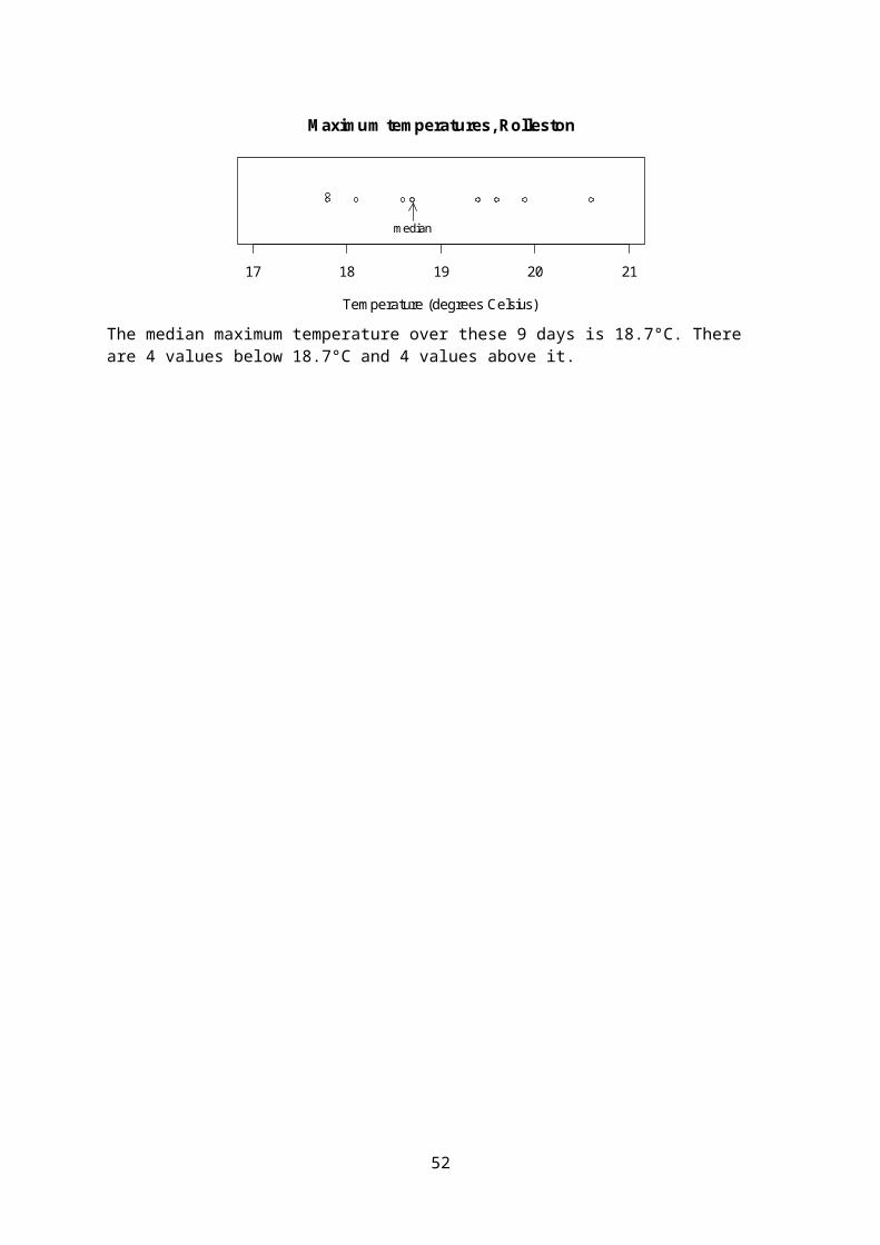
Alternative: pictogram, pictograph


Pie graphThere are two uses of pie graphs.

First, a graph for displaying the relative frequency distribution of a category variable in which a circle is divided into sectors, representing categories, so that the area of each sector represents the relative frequency of values in the category. See Example 1 below.

Second, a graph for displaying bivariate data; one category variable and one numerical variable. A circle is divided into sectors, representing categories, so that the area of each sector represents the value of the numerical variable for the sector as a percentage of the total value for all sectors. See Example 2 below.

For categories that do not have a natural ordering, it is desirable to order the categories from the largest sector area to the smallest.

Example 1

Students enrolled in an introductory Statistics course at the University of Auckland were asked to complete an online questionnaire. One of the questions asked them to enter their ethnicity. They chose from the following list: Chinese, Indian, Korean, Maori, New Zealand European, Other European, Pacific, Other. The 727 responses are displayed on the pie graph below.

52

NZ European

ChineseIndian

Korean

Other European

PacificMaori

Other

Ethnicity of university students

Example 2

World gold mine production for 2003 by country, based on official exports, is displayed on the bar graph below.

Alternatives: circle graph, pie chart


PlaceboA neutral treatment in an experiment that, to a person participating in the study, appears the same as the actual treatment.

Placebos are given to people in the control group so that reliable comparisons can be made between the treatment and control groups. People can experience positive outcomes from the psychological effect of believing they will improve because they have been given a treatment; the placebo effect. As part of determining whether a treatment is successful, researchers need to be able to see whether the effect due to a treatment is greater than the placebo effect.

Curriculum achievement objectives referencesStatistical investigation: Levels (7), (8)Statistical literacy: (Level 8)

Point estimateA number calculated from a random sample that is used as an approximate value for a population parameter.

Example

A sample proportion, calculated from a random sample taken from a population, is a point estimate of the population proportion.

Alternative: estimate

See: interval estimate

53

South Africa

Australia

United States

ChinaPeruRussia

Canada

Indonesia

Rest

Gold Production by Country, 2003

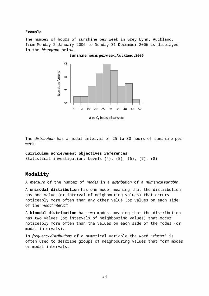
Curriculum achievement objectives referencesStatistical investigation: Levels (6), 7, (8)

Poisson distributionA family of theoretical distributions that is useful as a model for some discrete random variables. Each distribution in this family gives the probability of obtaining a specified number of occurrences of a phenomenon in a specified interval in time or space, under the following conditions:

On average, the phenomenon occurs at a constant rate, λ Occurrences of the phenomenon are independent of each other Two occurrences of the phenomenon cannot happen at exactly the same time or in exactly

the same place.

Each member of this family of distributions is uniquely identified by specifying λ. As such, λ, is the parameter of the Poisson distribution and the distribution is sometimes written as Poisson(λ).

Let random variable X represent the number of occurrences of a phenomenon that satisfies the conditions stated above. The probability of x occurrences is calculated by:

P(X = x) = for x = 0, 1, 2, ...

Example

A graph of the probability function for the Poisson distribution with λ = 3 is shown below.


PollA systematic collection of data about opinions on issues taken by questioning a sample of people taken from a population in order to determine the opinion distribution of the population.

Alternative: opinion poll

See: survey

54

0 1 2 3 4 5 6 7 8 9 10 11 12

Pro

babi

lity

0.00

0.05

0.10

0.15

0.20

0.25

Poisson distribution ( 3)

Curriculum achievement objectives referencesStatistical investigation: Levels (5), (6), (7), (8)Statistical literacy: Levels 7, 8

PopulationA collection of all objects or individuals of interest which have properties that someone wishes to record.

Sometimes a population is a collection of potential objects or individuals and, as such, does not physically exist but can be imagined to exist.

Example 1 (A real population)

All people aged 18 and over who were living in New Zealand on 8 November 2008.

Example 2 (An imagined population)

All possible 15-watt fluorescent light bulbs that could be produced by a manufacturing plant.

Curriculum achievement objectives referencesStatistical investigation: Levels 6, 7, (8)

Population distributionThe variation in the values of a variable if data has (or had) been obtained for every individual in the population.

Curriculum achievement objectives referencesStatistical investigation: Levels (5), (6), (7), (8)Probability: Levels (5), (6), (7), (8)

Population meanA measure of centre for a population distribution of a numerical variable. The population mean is the mean of all values of a numerical variable based on the collection of all objects or individuals of interest. It is the centre of mass of the values in a population distribution.

If the collection is finite then the population mean is obtained by adding all values in a set of values and then dividing this total by the number of values.

In many real situations the entire collection of values from a population is not available, for a variety of reasons. For example, the collection may be infinite or some objects or individuals may not be accessible. In such cases the value of the population mean is not known. The population mean may be estimated by taking a random sample of values from the population, calculating the sample mean and using this value as an estimate of the population mean.

The population mean is a number representing the centre of the population distribution and is therefore an example of a population parameter.

The Greek letter µ (mu) is the most common symbol for the population mean.

See: expected value (of a discrete random variable), mean, measure of centre

55


Population parameterA number representing a property of a population.

Common examples are the population mean, µ, the population proportion, π, and the population standard deviation, σ.

Population parameters, although fixed, are usually not known and are estimated by a statistic calculated from a random sample taken from the population. For example, a sample mean is an estimate of the population mean.


Population proportionA part of a population with a particular attribute, expressed as a fraction, decimal or percentage of the whole population.

For a finite population, the population proportion is the number of members in the population with a particular attribute divided by the number of members in the population.

In many real situations the whole population is not available to be checked for the presence of an attribute. In such cases the value of the population proportion is not known. The population proportion may be estimated by taking a random sample from the population, calculating the sample proportion and using this value as an estimate of the population proportion.

The population proportion is a number representing a part of a population and is therefore an example of a population parameter.

The Greek letter π (pi) is a common symbol for the population proportion.

See: proportion


Population standard deviationA measure of spread for a population distribution of a numerical variable that determines the degree to which the values differ from the population mean. If many values are close to the population mean then the population standard deviation is small and if many values are far from the population mean then the population standard deviation is large.

The square of the population standard deviation is equal to the population variance.

In many real situations the collection of all values from a population is not available, for a variety of reasons. For example, the collection may be infinite or some objects or individuals may not be accessible. In such cases the value of the population standard deviation is not known. The population standard deviation may be estimated by taking a random sample of values from the

56

population, calculating the sample standard deviation and using this value as an estimate of the population standard deviation.

The population standard deviation is a number representing the spread of the population distribution and is therefore an example of a population parameter.

The Greek letter σ (sigma) is the most common symbol for the population standard deviation.

See: measure of spread, population variance, standard deviation, standard deviation (of a discrete random variable)


Population varianceA measure of spread for a population distribution of a numerical variable that determines the degree to which the values differ from the population mean. If many values are close to the population mean then the population variance is small and if many values are far from the population mean then the population variance is large.

The positive square root of the population variance is equal to the population standard deviation.

In many real situations the collection of all values from a population is not available, for a variety of reasons. For example, the collection may be infinite or some objects or individuals may not be accessible. In such cases the value of the population variance is not known. The population variance may be estimated by taking a random sample of values from the population, calculating the sample variance and using this value as an estimate of the population variance.

The population variance is a number representing the spread of a population and is therefore an example of a population parameter.

The square of the population standard deviation is equal to the population variance, so σ2 (sigma squared) is the most common symbol for the population variance.

See: measure of spread, variance, variance (of a discrete random variable)


Precision (of an estimate)A measure of how close an estimate is expected to be to the true value of a population parameter. This measure is based on the degree of similarity among estimates of a population parameter, if the same sampling method were repeated over and over again.

Curriculum achievement objectives referencesStatistical investigation: Levels (7), 8Statistical literacy: (Level 8)

57

PredictionAn assessment of the value of a variable at some future point of time (for time-series data) or an assessment of the value of one variable based on knowing the value of the other variable (for bivariate numerical data).

Curriculum achievement objectives referencesStatistical investigation: Levels 7, 8

ProbabilityA number that describes the likely occurrence of an event, measured on a scale from 0 (impossible event) to 1 (certain event).

Curriculum achievement objectives referencesStatistical literacy: Level 6Probability: Levels 4, 5, 6, 7, 8

Probability activityAn activity that has a number of possible outcomes, none of which is certain to occur when a trial of the activity is performed.

Curriculum achievement objectives referencesStatistical literacy: Levels 1, 2, 3, 4, 5Probability: (All levels)

Probability density function (for a continuous random variable)A mathematical function that provides a model for the probability that a value of a continuous random variable lies within a particular interval. It is often useful to display this function as a graph, in which case this probability is the area between the graph of the function and the x-axis, bounded by the particular interval.

A probability density function has two further important properties:

1. Values of a probability density function are never negative for any value of the random variable.

2. The area under the graph of a probability density function is 1.

The use of ‘density’ in this term relates to the height of the graph. The height of the probability density function represents how closely the values of the random variable are packed at places on the x-axis. At places on the x-axis where the values are closely packed (dense) the height is greater than at places where the values are not closely packed (sparse).

More formally, probability density represents the probability per unit interval on the x-axis.

58

Example

Let X be a random variable with a normal distribution with a mean of 50 and a standard deviation of 15. The graph below shows the probability density function of X.

On the diagram below the shaded area equals the probability that X is between 15 and 30, i.e., P(15 < X < 30).


Probability function (for a discrete random variable)A mathematical function that provides a model for the probability of each value of a discrete random variable occurring.

For a discrete random variable that has a finite number of possible values, the function is sometimes displayed as a table, listing the values of the random variable and their corresponding probabilities.

A probability function has two important properties:

1. For each value of the random variable, values of a probability function are never negative, nor greater than 1.

2. The sum of the values of a probability function, taken over all of the values of the random variable, is 1.

59

0 25 50 75 100

Normal distribution ( 50, 15)

0 15 30 50 100

Normal distribution ( 50, 15)

Example 1

Let X be a random variable with a binomial distribution with n = 6 and π = 0.4. The probability function for random variable X is:

Probability of x successes in 6 trials, P(X = x) = for x = 0, 1, 2, 3, 4, 5, 6

where is the number of combinations of n objects taken x at a time.

A graph of this probability function is shown below.

Example 2

Imagine a probability activity in which a fair die is rolled and the number facing upwards is recorded. Let random variable X represent the result of any roll.

The probability function for random variable X can be written as:

x 1 2 3 4 5 6

P(X = x)

Alternative: probability model

See: model


ProportionA part of a distribution with a particular attribute, expressed as a fraction, decimal or percentage of the whole distribution.

See: sample proportion

Curriculum achievement objectives referencesStatistical investigation: Levels 5, (6), (7), 8

60

0 1 2 3 4 5 6

Pro

babi

lity

0.00

0.05

0.10

0.15

0.20

0.25

0.30


Qualitative dataData in which the values can be organised into distinct groups. These distinct groups must be chosen so they do not overlap and so that every value belongs to one and only one group, and there should be no doubt as to which one.

Example


Note: The Curriculum usage of category data is equivalent to qualitative data.

See: category data


Qualitative variableA property that may have different values for different individuals and for which these values can be organised into distinct groups. These distinct groups must be chosen so they do not overlap and so that every value belongs to one and only one group, and there should be no doubt as to which one.

Example


Note: The Curriculum usage of category variable is equivalent to qualitative variable.

See: category variable


Quantitative dataData in which the values result from counting or measuring. Measurement data are quantitative, as are whole-number data.

Alternative: numerical data

See: measurement data, whole-number data


Quantitative variableA property that may have different values for different individuals and for which these values result from counting or measuring. Measurement variables are quantitative, as are whole-number variables.

Alternative: numerical variable

61

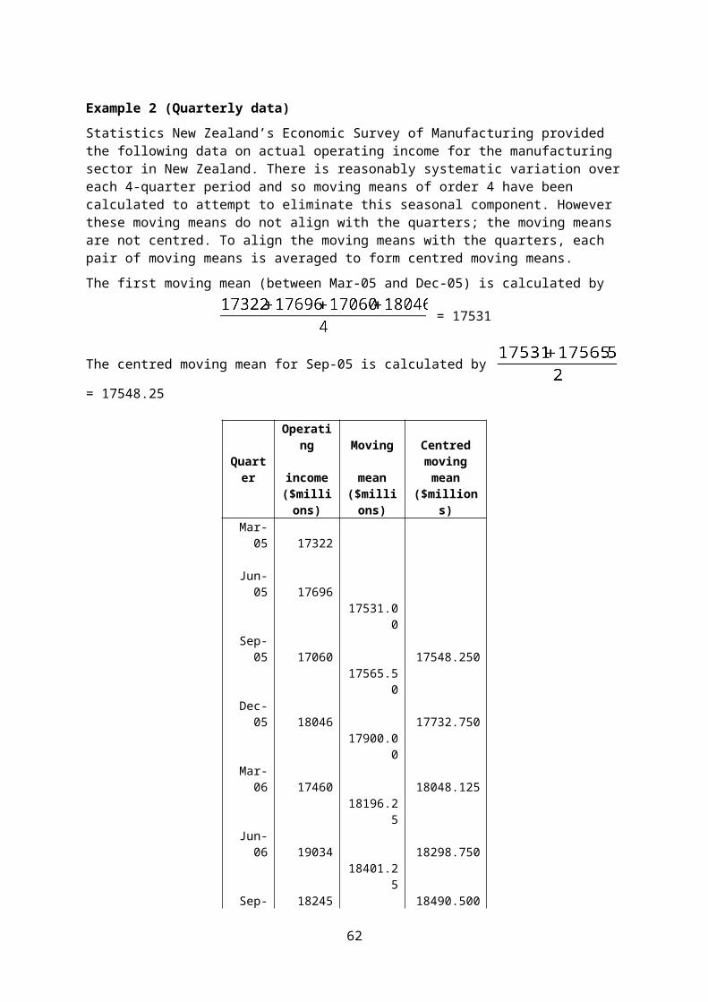
See: measurement variable, whole-number variable


QuartilesNumbers separating an ordered distribution into four groups, each containing (as closely as possible) equal numbers of values. The most common names for these three numbers, in order from lowest to highest, are lower quartile, median and upper quartile.

The lower quartile is a number that is a quarter of the way through the ordered distribution, from the lower end. The upper quartile is a number that is a quarter of the way through the ordered distribution, from the upper end.

There are several different methods for calculating quartiles. For reasonably small data sets it is recommended that the values are sorted into order (or displayed on a suitable graph) and then the median is calculated. This allows the distribution to be split into a ‘lower half’ and an ‘upper half’. The lower quartile is the median of the ‘lower half’ and the upper quartile is the median of the ‘upper half’. Use software for large data sets.

Note that different software may use different methods for calculating quartiles that may give different values for the quartiles. This is of no concern because in most cases any differences will be slight.

Example 1 (Odd number of values)

The maximum temperatures, in degrees Celsius (°C), in Rolleston for the first 9 days in November 2008 were: 18.6, 19.9, 20.6, 19.4, 17.8, 18.1, 17.8, 18.7, 19.6

Ordered values: 17.8, 17.8, 18.1, 18.6, 18.7, 19.4, 19.6, 19.9, 20.6

The median is 18.7°C.

The values in the ‘lower half’ are 17.8, 17.8, 18.1, 18.6. Their median is the mean of 17.8 and 18.1, which is 17.95. The lower quartile is 17.95°C.

The values in the ‘upper half’ are 19.4, 19.6, 19.9, 20.6. Their median is the mean of 19.6 and 19.9, which is 19.75. The upper quartile is 19.75°C.

The data and the quartiles are displayed on the dot plot below.

Notice that there are 2 values below the lower quartile, 2 values between the lower quartile and the median, 2 values between the median and the upper quartile and 2 values above the upper quartile.

62

17 18 19 20 21



lower median upperquartile quartile

Example 2 (Even number of values)


Ordered values: 17.8, 17.8, 18.1, 18.6, 18.7, 18.8, 19.4, 19.6, 19.9, 20.6

The median is 18.75°C.

The values in the ‘lower half’ are 17.8, 17.8, 18.1, 18.6, 18.7. Their median is 18.1. The lower quartile is 18.1°C.

The values in the ‘upper half’ are 18.8, 19.4, 19.6, 19.9, 20.6. Their median is 19.6. The upper quartile is 19.6°C.

The data and the quartiles are displayed on the dot plot below.

Notice that there are 2 values below the lower quartile, 2 values between the lower quartile and the median, 2 values between the median and the upper quartile and 2 values above the upper quartile.

See: median


Random sampleA sample in which all objects or individuals in the population have the same probability of being chosen in the sample.

A random sample can also be a number of independent values from the same theoretical distribution, without involving a real population.

See: simple random sample


Random samplingThe process of selecting a random sample.


63

17 18 19 20 21



lower median upperquartile quartile

Random variableA property that can have different values because there is an element of chance involved in obtaining any value for the property.

A random variable is often represented by an upper case letter, say X.

Example 1

The random selection of an individual from a population is subject to chance. The height of a selected individual will depend on the individual selected and is therefore a random variable. This may be written as, let X represent the height of a randomly selected individual.

Example 2

The random selection of 10 individuals from a population is subject to chance. The number of left-handed people in a sample of 10 individuals will depend on the individuals selected and is therefore a random variable. This may be written as, let X represent the number of left-handed people in a random selection of 10 individuals.

See: continuous random variable, discrete random variable

Curriculum achievement objectives referencesProbability: Levels (7), 8

RandomisationThe use of methods involving elements of chance, such as random numbers, to allocate individual units to groups.

Randomisation used in data collection

Randomisation is used in experiments by using methods involving elements of chance to allocate individual units to treatment groups. Further detail is provided in the paragraph on randomisation in the description of experimental design principles.

Randomisation forms the basis of many sampling methods, including random sampling, simple random sampling, cluster sampling and stratified sampling.

Randomisation used in statistical inference

Randomisation is used at Level Eight in a resampling method for making statistical inferences from data. This method is illustrated in the following two examples that compare two means. A summary of the method is provided after these two examples.

Example 1

An assertion is made that male University of Auckland students tend to reach faster driving speeds than female students. To investigate this, random samples of 20 male and 20 female University of Auckland students were asked how fast they had driven, to the nearest 10km/h.

The values obtained were:

Males: 130 120 120 140 140 120 120 120 170 160 110 150 210 240 200 140 150 200 240 140

64

Females: 100 170 140 120 120 120 120 90 120 100 130 120 120 130 120 120 110 100 130 120

The sample means are km/h for the males and km/h for the females. From this data, an estimate of the difference between the population mean fastest speeds for males and females is km/h.

A dot plot of the data is shown below.

Does the data provide any evidence to support the assertion? In other words, could a difference as big as the observed difference of 36.0 be produced just by chance?

If the numbers are considered as just showing the natural variability in fastest driving speeds among such university students, then would random allocation of the speeds from these two samples to the male and female groups often produce a difference in sample means as big as 36.0? If random allocation alone could easily produce a difference as big as 36.0 then the data cannot be interpreted as support that the mean fastest driving speed for males is greater than the mean for females.

The speeds from the two samples are combined and 20 of them are randomly allocated as speeds for the males, leaving the other 20 as speeds for the females. This is equivalent to assuming there is no link between fastest driving speed and gender. The difference in the sample means is an estimate produced by sampling variation alone. One such randomisation is shown below.

M M M M M M M M M M M M M M140 140 120 120 200 110 130 120 120 130 140 120 120 110M M M M M M F F F F F F F F

150 130 120 240 120 210 130 120 140 120 170 160 150 240F F F F F F F F F F F F

200 140 100 170 120 90 120 100 120 120 100 120

The sample means are km/h and km/h, with km/h.

Another random allocation of 20 (of the 40) as speeds for the males, leaving the other 20 as speeds for the females is shown below.

M M M M M M M M M M M M M M120 90 110 130 140 120 200 120 120 240 120 120 150 120M M M M M M F F F F F F F F

120 130 120 120 160 100 130 140 120 170 210 200 140 150F F F F F F F F F F F F

240 140 100 170 140 120 130 120 120 120 110 100

65

100 150 200

Fem

ale

Mal

e

Fastest driving speed by Gender

Fastest driving speed (km/h)

Gen

der

The sample means are km/h and km/h, with km/h.

Continuing this process for a total of 100 such random allocations produced differences in sample means shown in the dot plot below.

Of the 100 differences produced by sampling variation alone, none was as large as the observed difference of 36.0 km/h produced by the two samples. This shows that a difference of 36.0 km/h or larger is very unlikely to be produced by sampling variation alone when there is no link between fastest driving speed and gender. It can be concluded that the data provide very strong evidence that the mean fastest driving speed for male University of Auckland students is greater than that for females.

Note that the assertion was that the mean fastest driving speed for males is greater than that for females and so only positive differences of 36.0 or more were considered when forming the conclusion.

Example 2

Question: Is there a difference in the average daily number of text messages sent by male and female University of Auckland students? To investigate this, random samples of 20 male and 20 female University of Auckland students were asked how many text messages they typically sent in a day.

The values obtained were:

Males: 40 10 30 20 5 0 1 30 30 10 30 3 6 50 20 30 20 50 10 30

Females: 20 2 50 30 15 0 6 60 10 5 100 15 40 3 30 15 100 5 5 50

The sample means are messages per day for the males and messages per day for the females. From this data, an estimate of the difference between the population mean daily number of text messages for males and females is messages per day.

66

-30 -20 -10 0 10 20 30 40

Differences in sample means

Difference, male - female (km/h)

36.0

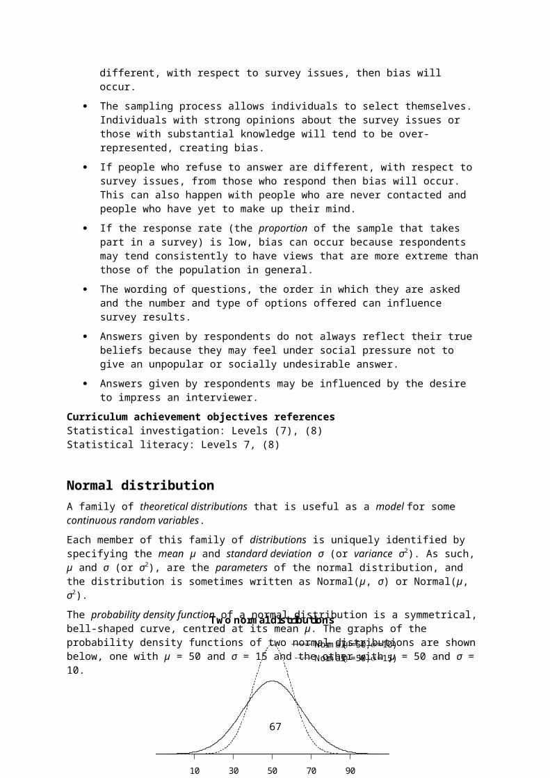
A dot plot of the data is shown below.

Does the data provide any evidence of a difference in the average daily number of text messages sent by male and female students? In other words, could a difference as big as the observed difference of –6.80 be produced just by chance?

If the numbers are considered as just showing the natural variability in daily numbers of text messages sent among such university students, then would random allocation of the number of messages from these two samples to the male and female groups often produce a difference as big as –6.80? If random allocation alone could easily produce a difference in sample means as big as –6.80 then the data cannot be interpreted as support that the mean daily number of text messages sent is different for males and females.

The numbers of messages from the two samples are combined and 20 of them are randomly allocated as daily numbers of text messages sent for the males, leaving the other 20 as daily numbers of text messages sent for the females. This is equivalent to assuming there is no link between daily number of text messages sent and gender. The difference in the sample means is an estimate produced by sampling variation alone. One such randomisation is shown below.

M M M M M M M M M M M M M M5 20 0 6 100 30 30 10 40 30 30 100 3 40M M M M M M F F F F F F F F50 50 50 15 0 20 10 30 20 1 30 30 10 30F F F F F F F F F F F F6 20 10 2 50 60 5 15 3 15 5 5

The sample means are and , with .

Another random allocation of 20 (of the 40) as daily numbers of text messages sent for the males, leaving the other 20 as daily numbers of text messages sent for the females is shown below.

M M M M M M M M M M M M M M30 0 30 60 5 10 30 50 50 5 10 20 30 40M M M M M M F F F F F F F F6 50 30 100 100 20 40 10 20 0 1 30 30 3F F F F F F F F F F F F50 10 20 2 15 6 15 3 30 15 5 5

The sample means are and , with .

67

0 20 40 60 80 100

Fem

ale

Mal

e

Daily number of text messages by Gender

Daily number of text messages

Gen

der

Continuing this process for a total of 100 such random allocations produced differences in sample means shown in the dot plot below.

Of the 100 differences produced by sampling variation alone, 52 (52%) were at least as far from zero as the difference of –6.80 produced by the two samples. This shows that a difference of –6.80 is a typical value produced by sampling variation alone when there is no link between daily number of text messages sent and gender. It can be concluded that the data provide no evidence that the mean daily number of text messages sent by male University of Auckland students is different from that for female students.

Note that the question was about a difference between the means for males and females and so positive and negative differences that are at least 6.80 from zero were considered when forming the conclusion.

Note: The principles explained in the above examples can also be applied to a difference between two proportions for category variables and to a slope of a fitted regression line for bivariate measurement variables.

Summary

Data are collected to investigate an assertion or a question, usually involving a comparison of a numerical variable between two categories of a category variable (i.e., that there is a link between the numerical variable and the category variable). An estimate of a population parameter is calculated from the data. This observed estimate is often a difference between means (as in the two examples) but could be a difference between two proportions or a slope of a fitted regression line.

Could an estimate as big as the observed estimate be produced just by chance?

To answer this question, the effect of sampling variation alone on the estimate needs to be considered when it is assumed that there is no link between the two variables. If random allocation alone could easily produce an estimate as big as the observed estimate then the data cannot be interpreted as support for the existence of a link between the two variables. Values of the numerical variable obtained from the data collection are randomly allocated to the two categories of the category variable. An estimate is calculated from this ‘resampling using randomisation’ process. This process is repeated many times to form a distribution of estimates under sampling variation alone.

By comparing the observed estimate with the distribution of estimates, an assessment can be made of the strength of evidence the data provide for the assertion or provide for a conclusion to the question. This assessment is made by looking at the percentage of estimates under sampling variation alone that are at least as far from zero as the observed estimate.

68

-20 -10 0 10 20

Differences in sample means

Difference, male - female

-6.80 6.80

Why are estimates that are at least as far from zero as the observed estimate considered?

If the observed estimate is a typical value of an estimate produced by sampling variation alone then it is quite believable there is no link between the variables. In this case, a relatively large percentage of estimates produced by sampling variation alone will be at least as far from zero as the observed estimate.

If the observed estimate is not a typical value of an estimate produced by sampling variation alone then it is difficult to believe there is no link between the variables. In this case, a relatively small percentage of estimates produced by sampling variation alone will be at least as far from zero as the observed estimate.

This makes the percentage of estimates produced by sampling variation alone that are at least as far from zero as the observed estimate an appropriate measure of the strength of evidence that there is a link between the two variables, with smaller percentages providing stronger evidence of a link.

Estimates produced by sampling variation alone are usually values of a continuous random variable (but the values are rounded). Because of the continuous nature of the values of these estimates, the percentage of estimates that are the same distance from zero as the observed estimate will almost always be small, causing this to be an inappropriate measure of the strength of evidence of a link.

See: resampling, strength of evidence

Curriculum achievement objectives referencesStatistical investigation: Levels (5), (6), (7), 8

RangeA measure of spread for a distribution of a numerical variable that is calculated as the difference between the largest and smallest values in the distribution.

The range is less useful than other measures of spread because it is strongly influenced by the presence of just one unusually large or small value; hence the range conveys only one aspect of the spread of the distribution. It is recommended that a graph of the distribution is used to check the appropriateness of the range as a measure of spread and to emphasise its meaning as a feature of the distribution.

Example


The largest value is 20.6°C and the smallest is 17.8°C.

The range of the maximum temperatures over these 10 days is 20.6°C – 17.8°C = 2.8°C

69

The data and the range are displayed on the dot plot below.

See: measure of spread


Re-categorising dataThe redefining of a variable in some way or the derivation of a new variable from one or more existing variables.

Example 1 (Redefining categories of a category variable)

Consider this question from a questionnaire:

From the given list of types of movies, select the one type that you like best.

Adventure □ Mystery □Comedy □ Romance □Horror □ Science fiction □Martial arts □ Thriller □Melodrama □ Tragedy □Other (please specify): ______________________________________

The data could initially be classified into the listed categories. If some categories had a relatively low frequency then it would be appropriate to re-categorise the data by combining some categories of a similar nature. This is called aggregation. For example; Horror, Mystery and Thriller could be aggregated to form a ‘Suspense’ category. Alternatively, if the ‘Other’ category had a relative high frequency then the specified responses may suggest some additional categories which could then be used to re-categorise the data.

Example 2 (Expressing the values of a numerical variable in a simpler way)

The values of a variable ‘Time’ could initially be recorded as the time from a stop-watch, say 2h 4m 32.4s. For explanation and analysis all values need to be converted to the time in seconds; 7472.4s for the value above.

70

17 18 19 20 21



range = 2.8

Example 3 (Deriving new variables from an existing variable)

From a variable ‘Date of Birth’ several new variables could be formed, such as ‘Age in Completed Years’, ‘Year of Birth’, ‘Day of Birth’, ‘Month of Birth’ or ‘Star Sign’.

Example 4 (Deriving a new variable from existing variables)

From the variables ‘Height’ and ‘Weight’ a new variable ‘Body Mass Index’ can be formed by calculating Weight/Height2, provided that weight is recorded in kilograms and height is recorded in metres.

Example 5 (Deriving a new variable from existing variables)

From the variables ‘Total Weekly Leisure Time’ and ‘Weekly Time Playing Sport’ a new variable ‘Percentage Sport Time’ can be formed by Weekly Time Playing Sport/Total Weekly Leisure Time × 100.


Regression lineA line that summarises the linear relationship (or linear trend) between the two variables in a linear regression analysis, from the bivariate data collected.

A regression line is an estimate of the line that describes the true, but unknown, linear relationship between the two variables. The equation of the regression line is used to predict (or estimate) the value of the response variable from a given value of the explanatory variable.

Example

The actual weights and self-perceived ideal weights of a random sample of 40 female students enrolled in an introductory Statistics course at the University of Auckland are displayed on the scatter plot below. A regression line has been drawn. The equation of the regression line ispredicted y = 0.6089x + 18.661 or predicted ideal weight = 0.6089 × actual weight + 18.661

71

50 60 70 80 90

5060

7080

90


Actual weight (kg)

Idea

l wei

ght (

kg)

estimated y = 0.6089x + 18.661

Alternatives: fitted line, line of best fit, trend line

See: least-squares regression line


RelationshipA connection between two variables, usually two numerical variables. Such a connection may not be evident until the data are displayed. A relationship between two variables is said to exist if the connection evident in a data display is so strong that it could not be explained as only due to chance.

Example 1 (Two numerical variables)

The actual weights and self-perceived ideal weights of a random sample of 40 female students enrolled in an introductory Statistics course at the University of Auckland are displayed on the scatter plot below (left). In general, as the values of actual weight increase the values of ideal weight increase. There is clearly a relationship between the variables actual weight and ideal weight.

The actual weights and number of countries visited (other than New Zealand) of a random sample of 40 male students enrolled in an introductory Statistics course at the University of Auckland are displayed on the scatter plot below (right). There is no clear connection between the variables actual weight and number of countries visited (other than New Zealand).

Example 2 (One numerical variable and one category variable)

The actual weights of random samples of 40 male and 40 female students enrolled in an introductory Statistics course at the University of Auckland are displayed on the dot plot below (left). On average, the actual weight of males is greater than that of females. There is clearly a relationship between the variables actual weight and gender.

The number of countries visited (other than New Zealand) by random samples of 40 male and 40 female students enrolled in an introductory Statistics course at the University of Auckland are

72

60 70 80 90 100 110

05

1015

20

Countries visited vs Actual weight, males

Actual weight (kg)

Num

ber

of c

ount

ries

visi

ted

50 60 70 80 90

5060

7080

90


Actual weight (kg)

Idea

l wei

ght (

kg)

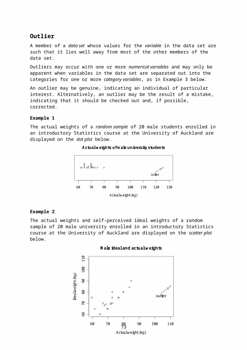
displayed on the dot plot below (right). The two sample distributions are quite similar indicating that there is no clear connection between the variables number of countries visited (other than New Zealand) and gender.

Example 3 (Two category variables)

The two sets of bar graphs below display data collected from a random sample of students studying an introductory Statistics course at the University of Auckland. They are enrolled in one of 3 courses; STATS 101, STATS 102 or STATS 108.

The proportions of each ethnic group in each course are displayed on the bar graphs on the left. The three distributions are sufficiently different to indicate that there is a relationship between the variables ethnicity and course.

The proportions of each ethnic group for males and females are displayed on the bar graphs on the right. The two distributions are quite similar indicating that there is no clear connection between the variables ethnicity and gender.

See: association

Curriculum achievement objectives referencesStatistical investigation: Levels 4, 5, 6, (7), (8)

73

0 5 10 15 20 25

Fem

ale

Mal

e

Countries visited by Gender

Number of countries visited

Gen

der

50 60 70 80 90 100 110

Fem

ale

Mal

e

Actual weight by Gender

Actual weight (kg)

Gen

der

Relative frequencyFor a whole-number variable in a data set, the number of times a value occurs divided by the total number of observations.

For a measurement variable in a data set, the number of occurrences in a class interval divided by the total number of observations.

For a category variable in a data set, the number of occurrences in a category divided by the total number of observations.

In other words, relative frequency =

See: frequency


Relative riskThe ratio of the risk (or probability) of an event for one group to the risk of the same event for a second group.

Example

The following data were collected on a random sample of students enrolled in a Statistics course at the University of Auckland.

AttendanceRegular Not regular Total

Course Pass 83 19 102result Fail 17 27 44

Total 100 46 146

The risk of failing for students with non-regular attendance= 4627

= 0.5870

The risk of failing for students with regular attendance= 10017

= 0.17

The relative risk of failing for students with non-regular attendance compared to those with regular

attendance = 170

58700.

. = 3.5

This can be interpreted as the risk of failing for students with non-regular attendance is about 3.5 times the risk of failing for students with regular attendance.

Curriculum achievement objectives referencesProbability: Levels 7, (8)

74

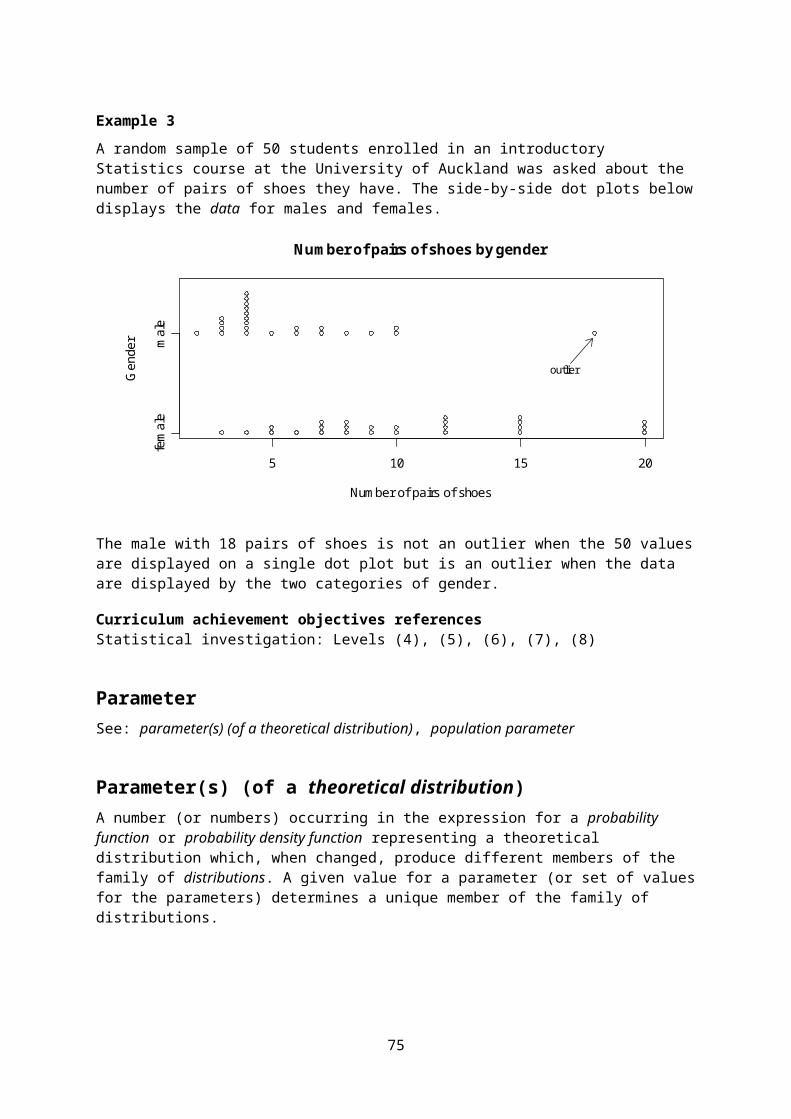
ResamplingA technique in which samples are taken repeatedly from an existing sample or existing samples.

Resampling using randomisation is a method used at Level Eight. Two examples of this method are provided in the description of randomisation and a summary of the method is given in the paragraphs below this paragraph.

Data are collected to investigate an assertion or a question, usually involving a comparison of a numerical variable between two categories of a category variable (i.e., that there is a link between the numerical variable and the category variable). An estimate of a population parameter is calculated from the data. This observed estimate is often a difference between means but could be a difference between two proportions or a slope of a fitted regression line.




See: randomisation, strength of evidence


Residual (in linear regression)The difference between an observed value of the response variable and the value of the response variable predicted from the regression line.

From bivariate data to be used for a linear regression analysis, consider one observation, . For this value of the explanatory variable, xi, the value of the response variable predicted from the regression line is , giving a point that is on the regression line. The residual for the

observation is .

Example

The actual weights and self-perceived ideal weights of a random sample of 40 female university students enrolled in an introductory Statistics course at the University of Auckland are displayed on the scatter plot below. A regression line has been drawn. The equation of the regression line ispredicted y = 0.6089x + 18.661 or predicted ideal weight = 0.6089 × actual weight + 18.661

Consider the female whose actual weight is 72kg and whose self-perceived ideal weight is 70kg.

Her predicted ideal weight is 0.6089 × 72 + 18.661 = 62.5kg

75

The residual for this observation is 70kg – 62.5kg = 7.5kg

This is also displayed on the scatter plot.

Alternative: prediction error


Response variableThe variable, of the two variables in bivariate data, which may be affected by the other variable, the explanatory variable.

If the bivariate data result from an experiment then the response variable is the one that is observed in response to the experimenter having manipulated or selected the value of the explanatory variable.

In a scatter plot, as part of a linear regression analysis, the response variable is placed on the y-axis (vertical axis).

Alternatives: dependent variable, outcome variable, output variable


76

50 60 70 80 90

5060

7080

90


Actual weight (kg)

Idea

l wei

ght (

kg)

(72,62.5)

(72,70)

residual

RiskAn alternative name for probability. The risk of an event occurring is the probability of the event occurring and is mainly used when the event is related to a health issue or is an undesirable event.

Example

The following data were collected on a random sample of students enrolled in a Statistics course at the University of Auckland.

AttendanceRegular Not regular Total

Course Pass 83 19 102result Fail 17 27 44

Total 100 46 146

Based on this sample of students, the risk of failing = 14644

= 0.30

The risk of failing for students with regular attendance= 10017

= 0.17


SampleA group of objects, individuals or values selected from a population. The intention is for this sample to provide estimates of population parameters.

See: cluster sampling, random sample, simple random sample, stratified sampling, systematic sampling

Curriculum achievement objectives referencesStatistical investigation: Levels 5, (6), (7), (8)Probability: Levels 6, (7)

Sample distributionThe variation in the values of a variable in data obtained from a sample.

For whole-number data, a sample distribution is often displayed, in a table, as a set of values and their corresponding frequencies, or on an appropriate graph.

For measurement data, a sample distribution is often displayed, in a table, as a set of intervals of values (class intervals) and their corresponding frequencies, or on an appropriate graph.

For category data, a sample distribution is often displayed, in a table, as a set of categories and their corresponding frequencies, or on an appropriate graph.

Alternative: empirical distribution

See: experimental distribution

77


Sample meanA measure of centre for the distribution of a sample of numerical values. The sample mean is the centre of mass of the values in their distribution.

If the n values in a sample are x1, x2, ... , xn, then the sample mean is calculated by adding the values in the sample are then dividing this total by the number of values. In symbols, the sample mean, ,

is calculated by .

For large samples it is recommended that a calculator or software is used to calculate the mean.

The sample mean is a (sample) statistic and is therefore an estimate of the population mean.

See: mean


Sample proportionA part of a sample with a particular attribute, expressed as a fraction, decimal or percentage of the whole sample.

A common symbol for the sample proportion is p.

Example

Suppose the attribute of interest was left-handedness and that a random sample of 10 people contained 3 left-handed people.

The sample proportion is or 0.3 or 30%.

See: proportion

Curriculum achievement objectives referencesStatistical investigation: Levels (6), (7), 8

Sample sizeThe number of objects, individuals or values in a sample.

Typically, a larger sample size leads to an increase in the precision of a statistic as an estimate of a population parameter.

The most common symbol for sample size is n.

Curriculum achievement objectives referencesStatistical investigation: Levels (5), (6), 7, (8)Probability: Levels 6, (7)

78

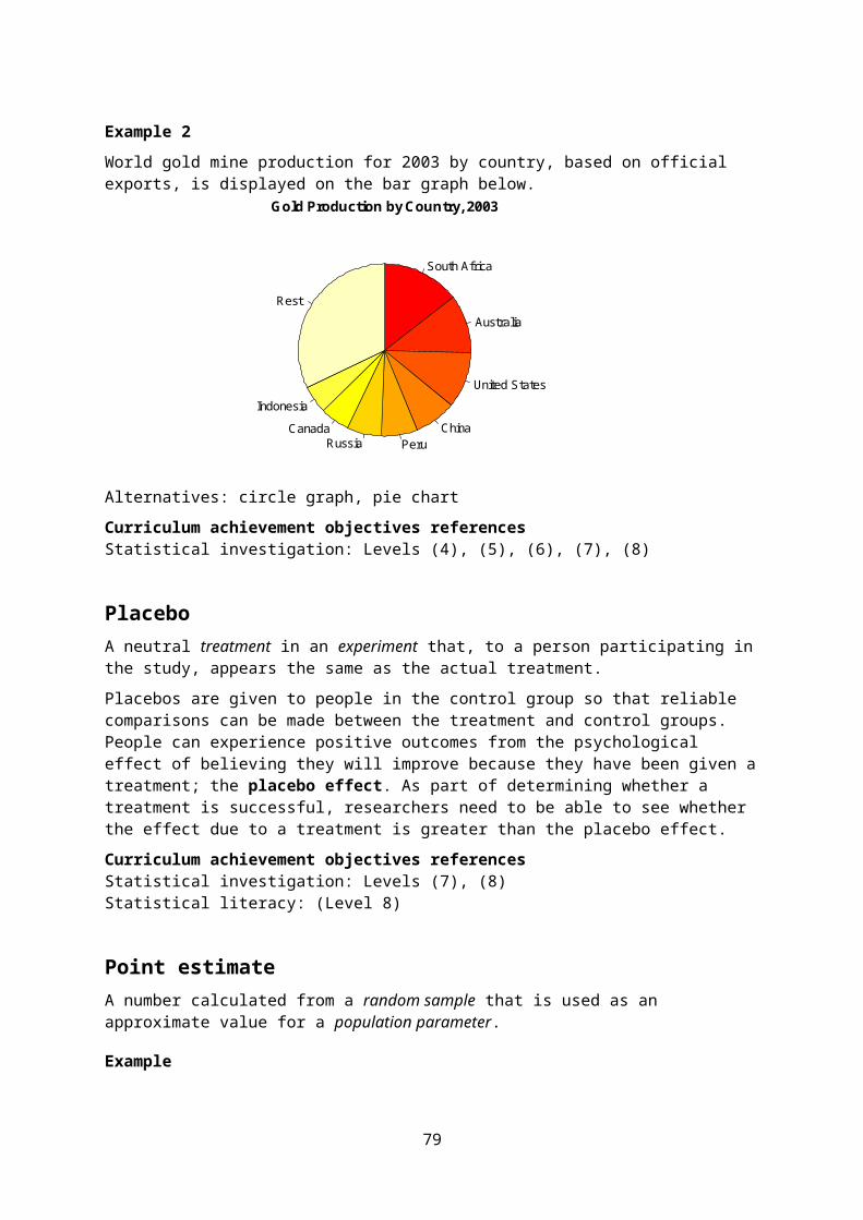
Sample spaceThe set of all of the possible outcomes for a probability activity or a situation involving an element of chance.

For discrete situations the sample space can be listed.

Note that a sample space can often be described in several different ways.

Example 1

In a situation where a person will be selected and their eye colour recorded, a sample space is blue, grey, green, hazel, brown. Each person’s eye colour must belong to exactly one of these categories.

Example 2

In a situation where the gender of the child is recorded in birth order, a sample space is: (BBB, BBG, BGB, BGG, GBB, GBG, GGB, GGG).

A different sample space could be: 3 boys, exactly 2 boys, exactly 1 boy, no boys.

A different sample space again could be: more boys than girls, more girls than boys.

Curriculum achievement objectives referencesProbability: Levels (4), (5), (6), (7), 8

Sample standard deviationA measure of spread for a distribution of a sample of numerical values that determines the degree to which the values differ from the sample mean.

It is calculated by taking the square root of the average of the squares of the deviations of the values from their sample mean.

It is recommended that a calculator or software is used to calculate the sample standard deviation.

The square of the sample standard deviation is equal to the sample variance.

A common symbol for the sample standard deviation is s.

The sample standard deviation is a (sample) statistic and is therefore an estimate of the population standard deviation.

See: measure of spread, sample variance, standard deviation


Sample statisticA number that is calculated from a sample of numerical values.

A sample statistic gives an estimate of the corresponding value from the population from which the sample was taken. For example, a sample mean is an estimate of the population mean.

See: statistic

79

Curriculum achievement objectives referencesStatistical investigation: Levels (6), 7, (8)

Sample statisticsNumbers calculated from a sample of numerical values that are used to summarise the sample. The statistics will usually include at least one measure of centre and at least one measure of spread.

Alternative: numerical summary

See: descriptive statistics, summary statistics


Sample varianceA measure of spread for a distribution of a sample of numerical values that determines the degree to which the values differ from the sample mean.

It is calculated by the average of the squares of the deviations of the values from their sample mean.

The positive square root of the sample variance is equal to the sample standard deviation.

It is recommended that a calculator or software is used to calculate the sample variance. On a calculator the square of the standard deviation will give the variance.

A common symbol for the sample variance is s2.

The sample variance is a (sample) statistic and is therefore an estimate of the population variance.

See: measure of spread, sample standard deviation, variance


Sampling distributionA theoretical distribution for the variation in the values of a sample statistic, such as a sample mean, based on samples of a fixed size, n. When the sample statistic is the sample mean, the sampling distribution is called the sampling distribution of the sample mean.

Example

Consider the mean of a random sample of 20 values taken from a population. Suppose that several more random samples of 20 values were taken from the same population and the sample mean for each sample was calculated. The values of these sample means would differ from sample to sample (illustrating sampling variation). Imagine repeating this process over and over again, without end. The variation in the values of these sample means is the sampling distribution of the sample mean.

See: central limit theorem


80

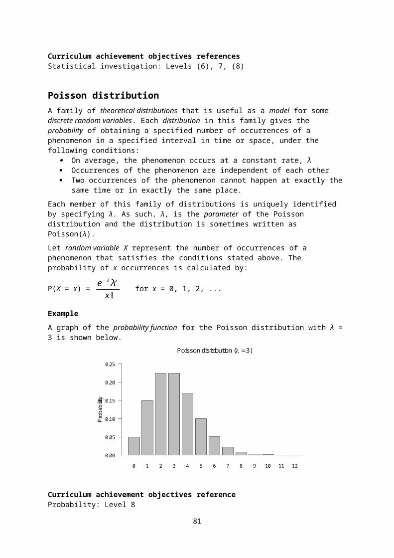
Sampling errorThe error caused because data are collected from part of a population rather than the whole population.

An estimate of a population parameter, such as a sample mean or sample proportion, is different for different samples (of the same size) taken from the population. Sampling error is one of two reasons for the difference between an estimate and the true, but unknown, value of the population parameter. The other reason is non-sampling error.

The error for a given sample is unknown but when sampling is random, the size of the sampling error can be estimated by calculating the margin of error.

See: margin of error, non-sampling error

Curriculum achievement objectives referencesStatistical investigation: Levels (5), (6), (7), (8)Statistical literacy: Levels 7, (8)

Sampling variationThe variation in a sample statistic from sample to sample.

Suppose a sample is taken and a sample statistic, such as a sample mean, is calculated. If a second sample of the same size is taken from the same population, it is almost certain that the sample mean calculated from this sample will be different from that calculated from the first sample. If further sample means are calculated, by repeatedly taking samples of the same size from the same population, then the differences in these sample means illustrate sampling variation.

Alternative: chance variation

Curriculum achievement objectives referencesStatistical investigation: Levels (5), (6), (7), (8)Probability: Levels (3), (4), (5), (6)

ScatterFor bivariate numerical data, the variation (in the vertical direction) of the values of the variable plotted on the y-axis of a scatter plot.

In linear regression, scatter is the variation (in the vertical direction) of the values of the response variable from the regression line.


81

Scatter plotA graph for displaying a pair of numerical variables. The graph has two axes, one for each variable, and points are plotted to show the values of these two variables for each of the individuals.

A scatter plot is essential for exploring the relationship that may exist between the two variables and for revealing the features of this relationship.

In linear regression, at Level Eight, one of the two variables is regarded as the explanatory variable and the other variable as the response variable. In this case the explanatory variable is plotted on the horizontal axis (x-axis) and the response variable is plotted on the vertical axis (y-axis).

When fitting models to data, as in linear regression, a scatter plot is essential for assessing how useful the fitted model may be.

Example

The actual weights and self-perceived ideal weights of a random sample of 40 female university students enrolled in an introductory Statistics course at the University of Auckland are displayed on the scatter plot below.

Alternatives: scatter diagram, scattergram, scatter graph


Seasonal component (for time-series data)Variations in time-series data that repeat more or less regularly which are due to the effect of the seasons of the year, or to the effect of other periodic influences such as systematic patterns within each week or within each day.

Alternative: seasonality



82

50 60 70 80 90

5060

7080

90


Actual weight (kg)

Idea

l wei

ght (

kg)

Seasonally adjusted dataTime-series data which have had the seasonal component removed. In seasonally adjusted data the effect of regular seasonal phenomena has been removed.


the smoothed series = T + C andthe seasonally adjusted series = T + C + I.

Example

Statistics New Zealand’s Economic Survey of Manufacturing provided the following data on actual operating income for the manufacturing sector in New Zealand. Centred moving means have been calculated. For the quarters with centred moving means the individual seasonal effect is calculated by:

Operating income (raw data) – (centred) moving mean

The overall seasonal effect for each quarter is estimated by averaging the individual seasonal effects. The two individual seasonal effects for March quarters are –588.125 and –561.75. The mean of these 2 values is –574.938. The other estimated overall seasonal effects are shown in the second table below.

Seasonally adjusted data is calculated by:Operating income (raw data) – estimated overall seasonal effect

The calculation for the Mar-05 quarter is 17322 – (–574.938) = 17896.938

Operating Centred Individual SeasonallyQuarter income moving mean seasonal adjusted

($millions) ($millions) effect ($millions)Mar-05 17322 17896.938Jun-05 17696 17097.875Sep-05 17060 17548.250 -488.250 17426.875Dec-05 18046 17732.750 313.250 17773.125Mar-06 17460 18048.125 -588.125 18034.938Jun-06 19034 18298.750 735.250 18435.875Sep-06 18245 18490.500 -245.500 18611.875Dec-06 18866 18633.500 232.500 18593.125Mar-07 18174 18735.750 -561.750 18748.938Jun-07 19464 19003.000 461.000 18865.875Sep-07 18633 18999.875Dec-07 20616 20343.125

Individual and estimated overall seasonal effectsMar Jun Sep Dec

Individual -588.125 735.250 -488.250 313.250-561.750 461.000 -245.500 232.500

Overall -574.938 598.125 -366.875 272.875

83

The raw data and the seasonally adjusted data are displayed below. Note that M, J, S and D indicate quarter years ending in March, June, September and December respectively.


Simple random sampleA sample in which, at any stage of the sampling process, each object or individual (which has not been chosen) in the population has the same probability of being chosen in the sample.

In a simple random sample an object or individual in the population can be chosen once, at most. This is often called sampling without replacement.

See: random sample


84

15

16

17

18

19

20

21

22


Quarter

Ope

ratin

g in

com

e ($

billio

ns)

S-0

2D

-02

M-0

3J-

03S

-03

D-0

3M

-04

J-04

S-0

4D

-04

M-0

5J-

05S

-05

D-0

5M

-06

J-06

S-0

6D

-06

M-0

7J-

07S

-07

D-0

7M

-08

J-08

S-0

8

Operating incomeSeasonally adjusted

SimulationA technique for imitating the behaviour of a situation that involves elements of chance or a probability activity. The technique uses tools such as coins, dice, random numbers from a calculator, random numbers from random number tables, and random numbers generated by computers.

Example 1

A coin can be used to simulate the outcomes of three-child families, assuming that a boy and a girl are equally likely to occur. If a head results from the coin toss then a boy is the simulated birth outcome and if a tail results then a girl is the simulated birth outcome. A group of three coin tosses simulates an outcome of a three-child family. The simulation is continued until the required number of trials has been performed.

Suppose the results of 90 coin tosses and therefore 30 simulated trials of three-child families were:

HHT TTT HHT HTT HHT TTT THT TTH THT THT THT TTT HTH HTH HHH THT THT THH TTT HHH HHT TTH THT THH HTT THH THT HTH THH HHH

Trials:BBG GGG BBG BGG BBG GGG GBG GGB GBG GBG GBG GGG BGB BGB BBB GBG GBG GBB GGG BBB BBG GGB GBG GBB BGG GBB GBG BGB GBB BBB

The experimental distribution for the variable that lists numbers of boys and girls in the family is shown in the frequency table or one-way table below:

Combination 3 boys 2 boys and 1 girl 1 boy and 2 girls 3 girlsFrequency 3 11 12 4

Example 2

In a game of tennis one player from School A is to play one player from School B. School A has 3 players to choose from (C, D and E) and School B has 2 players to choose from (F and G). For School A, the probabilities of C, D or E being selected are 0.6, 0.3 and 0.1 respectively. For school B, the probabilities of F or G being selected are 0.7 and 0.3 respectively.

Simulate 25 performances (or trials) of this activity.

Suppose the random numbers to be used, starting at the beginning of this list, were:

71578 81355 39007 60764 19852 87652 50354 22183 14935 09519

Consider the digits in pairs.

The first digit will decide the player for School A. If it is 0, 1, 2, 3, 4 or 5 then player C is chosen; if it is 6, 7 or 8 then player D is chosen; if it is 9 then player E is chosen.

85

The second digit will decide the player for School B. If it is 0, 1, 2, 3, 4, 5 or 6 then player F is chosen; if it is 7, 8 or 9 then player G is chosen.

Trial Pair Combination Trial Pair Combination1 71 D plays F 14 76 D plays F2 57 C plays G 15 52 C plays F3 88 D plays G 16 50 C plays F4 13 C plays F 17 35 C plays F5 55 C plays F 18 42 C plays F6 39 C plays G 19 21 C plays F7 00 C plays F 20 83 D plays F8 76 D plays F 21 14 C plays F9 07 C plays G 22 93 E plays F

10 64 D plays F 23 50 C plays F11 19 C plays G 24 95 E plays F12 85 D plays F 25 19 C plays G13 28 C plays G

The experimental distribution for the variable that lists pairs of players is shown in the frequency table or one-way table below:

Combination C plays F C plays G D plays F D plays G E plays F E plays GFrequency 10 6 6 1 2 0


SkewnessA lack of symmetry in a distribution of a numerical distribution in which the values on one side of the distribution tend to be further from the centre of the distribution than values on the other side.

If the smaller values of a distribution tend to be further from the centre of the distribution than the larger values, the distribution is said to have negative skew or to be skewed to the left (or left-skewed).

If the larger values of a distribution tend to be further from the centre of the distribution than the smaller values, the distribution is said to have positive skew or to be skewed to the right (or right-skewed).

86

Example 1

The actual weights of a random sample of 50 female university students enrolled in an introductory Statistics course at the University of Auckland are displayed on the dot plot below. The sample distribution is skewed to the right or positively skewed.

Example 2

The bar graph displays the probability function of the binomial distribution with n = 10 and π = 0.8. The theoretical distribution is skewed to the left or negatively skewed.


Smoothing dataA process of removing fluctuations from time-series data so that the resulting series shows much less variation, and is therefore smoother.

At Level Eight, moving averages (usually moving means) are used as a method of smoothing time-series data.

See: moving averages, moving mean, time-series data


87

30 40 50 60 70 80 90 100

Actual weights of female university students

Actual weight (kg)

0 1 2 3 4 5 6 7 8 9 10

Pro

babi

lity

0.00

0.05

0.10

0.15

0.20

0.25

0.30


Sources of variationThe reasons for differences seen in the values of a variable. Some of these reasons are summarised in the following paragraphs.

Variation is present everywhere and is in everything. When the same variable is measured for different individuals there will be differences in the measurements, simply due to the fact that individuals are different. This can be thought of as individual-to-individual variation and is often described as natural or real variation.

Repeated measurements on the same individual may vary because of changes in the variable being measured. For example, an individual’s blood pressure is not exactly the same throughout the day. This can be thought of as occasion-to-occasion variation.

Repeated measurements on the same individual may vary because of some unreliability in the measurement device, such as a slightly different placement of a ruler when measuring. This is often described as measurement variation.

The difference in measurements of the same quantity for different individuals, apart from natural variation, could be due to the effect of one or more other factors. For example, the difference in growth of two tomato plants from the same packet of seeds planted in two different places could be due to differences in the growing conditions at those places, such as soil fertility or exposure to sun or wind. Even if the two seeds were planted in the same garden there could be differences in the growth of the plants due to differences in soil conditions within the garden. This is often described as induced variation.

Variation occurs in all sampling situations. Suppose a sample is taken and a sample statistic, such as a sample mean, is calculated. If a second sample of the same size is taken from the same population, it is almost certain that the sample mean calculated from this sample will be different from that calculated from the first sample. If further sample means are calculated, by repeatedly taking samples of the same size from the same population, then the differences in these sample means illustrate sampling variation.

Curriculum achievement objectives referencesStatistical investigation: Levels 5, 6, (7), (8)

SpreadThe degree to which values in a distribution of a numerical variable differ from each other.

Alternative: dispersion

See: variability, variation


88

Standard deviationA measure of spread for a distribution of a numerical variable that determines the degree to which the values differ from the mean. If many values are close to the mean then the standard deviation is small and if many values are far from the mean then the standard deviation is large.

It is calculated by taking the square root of the average of the squares of the deviations of the values from their mean.

It is recommended that a calculator or software is used to calculate the standard deviation.

The standard deviation can be influenced by unusually large or unusually small values. It is recommended that a graph of the distribution is used to check the appropriateness of the standard deviation as a measure of spread and to emphasise its meaning as a feature of the distribution.

The square of the standard deviation is equal to the variance.

Note that calculators have two keys for the two different ways the standard deviation can be calculated. One way divides the sum of the squared deviations by the number of values before taking the square root. The other way divides the sum of the squared deviations by one less than the number of values before taking the square root. At school level, it does not really matter which key is used because for all but quite small data sets the two values for the standard deviation will be similar. Software tends to use the calculation that divides by one less than the number of values; but some offer both ways. The first way (dividing by the number of values) is better when there are values for all members of a population and the second way is better when the values are from a sample.

Example


The standard deviation using division by 9 (one less than the number of values) is 0.93°C.

The standard deviation using division by 10 (the number of values) is 0.88°C.

The data, the mean and the standard deviation are displayed on the dot plot below.

See: measure of spread, population standard deviation, sample standard deviation, variance


89

17 18 19 20 21



meanstandard standarddeviation deviation

Standard deviation (of a discrete random variable)A measure of spread for a distribution of a random variable that determines the degree to which the values differ from the expected value.

The standard deviation of random variable X is often written as σ or σX.

For a discrete random variable the standard deviation is calculated by summing the product of the square of the difference between the value of the random variable and the expected value, and the associated probability of the value of the random variable, taken over all of the values of the random variable, and finally taking the square root.

In symbols, σ =

An equivalent formula is, σ =

The square of the standard deviation is equal to the variance, Var(X) = σ 2.

Example


x 0 1 2 3P(X = x) 0.1 0.2 0.4 0.3

Using σ =

µ = 0 x 0.1 + 1 x 0.2 + 2 x 0.4 + 3 x 0.3

= 1.9

σ =

=

= 0.94

Using σ =

E(X) = 0 x 0.1 + 1 x 0.2 + 2 x 0.4 + 3 x 0.3

= 1.9

E(X2) = 02 × 0.1 + 12 × 0.2 + 22 × 0.4 + 32 × 0.3

= 4.5

σ =

= 0.94

90

A bar graph of the probability function, with the mean and standard deviation labelled, is shown below.

See: population standard deviation, standard deviation


Standard errorA measure of spread for the values of an estimate, if the sampling method were repeated over and over. As such, a standard error is a measure of the precision of an estimate.

Standard error is used with two similar, but different, meanings. The first meaning is the standard deviation of an estimate. The second meaning is an estimated standard deviation of an estimate.

Estimates vary from sample to sample so that, in general, an estimate is a random variable. The first meaning of standard error is the standard deviation of the random variable representing an estimate.

The standard deviation of the random variable representing an estimate is usually not useful because it depends on the (usually) unknown value of a population parameter. The second meaning of standard error is an estimated standard deviation of the random variable representing an estimate.

Unfortunately, both meanings are in common usage.

Example

Consider the sampling distribution of the sample mean and let random variable represent the sample mean.

The standard deviation of is

First meaning: The standard error of the sample mean is .

The population standard deviation, σ, is not known.

Suppose for a sample of size 20, and s = 13.63.

By replacing σ with s the standard error is estimated to be

91

0 1 2 3

Pro

babi

lity

0.0

0.1

0.2

0.3

0.4

Second meaning: By replacing σ with s the standard error of the sample mean is

The standard error of the sample mean is

Curriculum achievement objectives referencesStatistical investigation: (Level 8)Statistical literacy: (Level 8)

Standard normal distributionThe normal distribution with a mean of 0 and a standard deviation of 1.


StatisticA number that is calculated from numerical data.

Statistics listed in this glossary are: mean, median, mode, standard deviation, variance, interquartile range, range, lower quartile, upper quartile.

Alternative: summary statistic

See: sample statistic

Curriculum achievement objectives referencesStatistical investigation: Levels (6), (7), (8)Statistical literacy: Levels 6, (7), (8)

Statistical enquiry cycleA cycle that is used to carry out a statistical investigation. The cycle consists of five stages: Problem, Plan, Data, Analysis, Conclusion. The cycle is sometimes abbreviated to the PPDAC cycle.

The problem section is about formulating a statistical question, what data to collect, who to collect it from and why it is important.

The plan section is about how the data will be gathered.

92

Standard normal distribution

-3 -2 -1 0 1 2 3

The data section is about how the data is managed and organised.

The analysis section is about exploring and analysing the data, using a variety of data displays and numerical summaries, and reasoning with the data.

The conclusion section is about answering the question in the problem section and giving reasons based on the analysis section.

Reference: www.censusatschool.org.nz/2005/documents/how-kids-learn.pdf

Curriculum achievement objectives referencesStatistical investigation: All levels

Statistical inferenceThe process of drawing conclusions about population parameters based on a sample taken from the population.

Example 1

Using a sample mean calculated from a random sample taken from a population to estimate the population mean is an example of statistical inference.

Example 2

Using data from a random sample taken from a population to obtain a 95% confidence interval for the population proportion is an example of statistical inference.

Alternative: inference

Curriculum achievement objectives referencesStatistical investigation: Levels 6, 7, 8

Statistical investigationAn information gathering and learning process that is undertaken to seek meaning from and to learn more about any aspect of the real world, as well as to help make informed decisions and take informed actions. Statistical investigations should use the statistical enquiry cycle (Problem, Plan, Data, Analysis, Conclusion).

Reference: www.censusatschool.org.nz/2005/documents/statistical-investigation.pdf

See: statistical enquiry cycle

Curriculum achievement objectives referencesStatistical investigation: All levelsStatistical literacy: Levels 1, 2, 3, 4, 5

93

http://www.censusatschool.org.nz/2005/documents/statistical-investigation.pdf

http://www.censusatschool.org.nz/2005/documents/how-kids-learn.pdf

Stem-and-leaf plotA graph for displaying the distribution of a numerical variable that is similar to a histogram but retains some information about individual values.

Ideally the numbers in the ‘stem’ represent the highest place-value digit in the values and the ‘leaves’ display the second highest place-value digits in each individual value.

To compare the distribution of a numerical variable for two categories of a category variable, a back-to-back stem-and-leaf plot can be drawn, in which the stem is placed at the centre and the leaves for the values of the numerical variable for one category are drawn on one side of the stem and the leaves for the other category are drawn on the other side.

Stem-and-leaf plots are particularly useful when the number of values to be plotted is not large.

Example 1

The actual weights of a random sample of 40 male university students enrolled in an introductory Statistics course at the University of Auckland are displayed on the stem-and-leaf plot below.

Actual weights of male university students (kg)

5 | 1577 6 | 0000002223557889 7 | 00012233455 8 | 00344589999 9 | 008 10 | 0009 11 | 12 | 0

The stem unit is 10kg

Example 2 (Back-to-back stem-and-leaf plot)

The actual weights of random samples of 40 female and 40 male university students enrolled in an introductory Statistics course at the University of Auckland are displayed on the back-to-back stem-and-leaf plot below.

Actual weights of university students (kg)

Females Males

9 | 3 | 99988876 | 4 | 8876665555554432220000 | 5 | 1577 88542200 | 6 | 0000002223557889 5200 | 7 | 00012233455 5550 | 8 | 00344589999 330 | 9 | 008 | 10 | 0009 | 11 | | 12 | 0

The stem unit is 10kg

94

Alternative: stem plot


Stratified samplingA method of sampling in which the population is split into non-overlapping groups (the strata), with the groups having different characteristics that are known for the whole population. A simple random sample is taken from each stratum.

Example

Consider obtaining a sample of students from a secondary school with students from Year 9 to Year 13. The year levels are suitable strata, and the simple random samples taken from each year level form the sample.


Strength of evidenceAn assessment of how well data, collected to investigate an assertion or question, support the assertion or support a conclusion to the question. The assertion or question usually involves a comparison of a numerical variable between two categories of a category variable (i.e., that there is a link between the numerical variable and the category variable).

Data are collected to investigate the assertion or question. An estimate of a population parameter is calculated from the data. This observed estimate is often a difference between means but could be a difference between two proportions or a slope of a fitted regression line.




If less than about 0.1% of the estimates produced by random allocation alone are at least as far from zero as the observed estimate then the data provide very strong evidence of a link between the two variables.

If about 1% of the estimates produced by random allocation alone are at least as far from zero as the observed estimate then the data provide strong evidence of a link between the two variables.

95

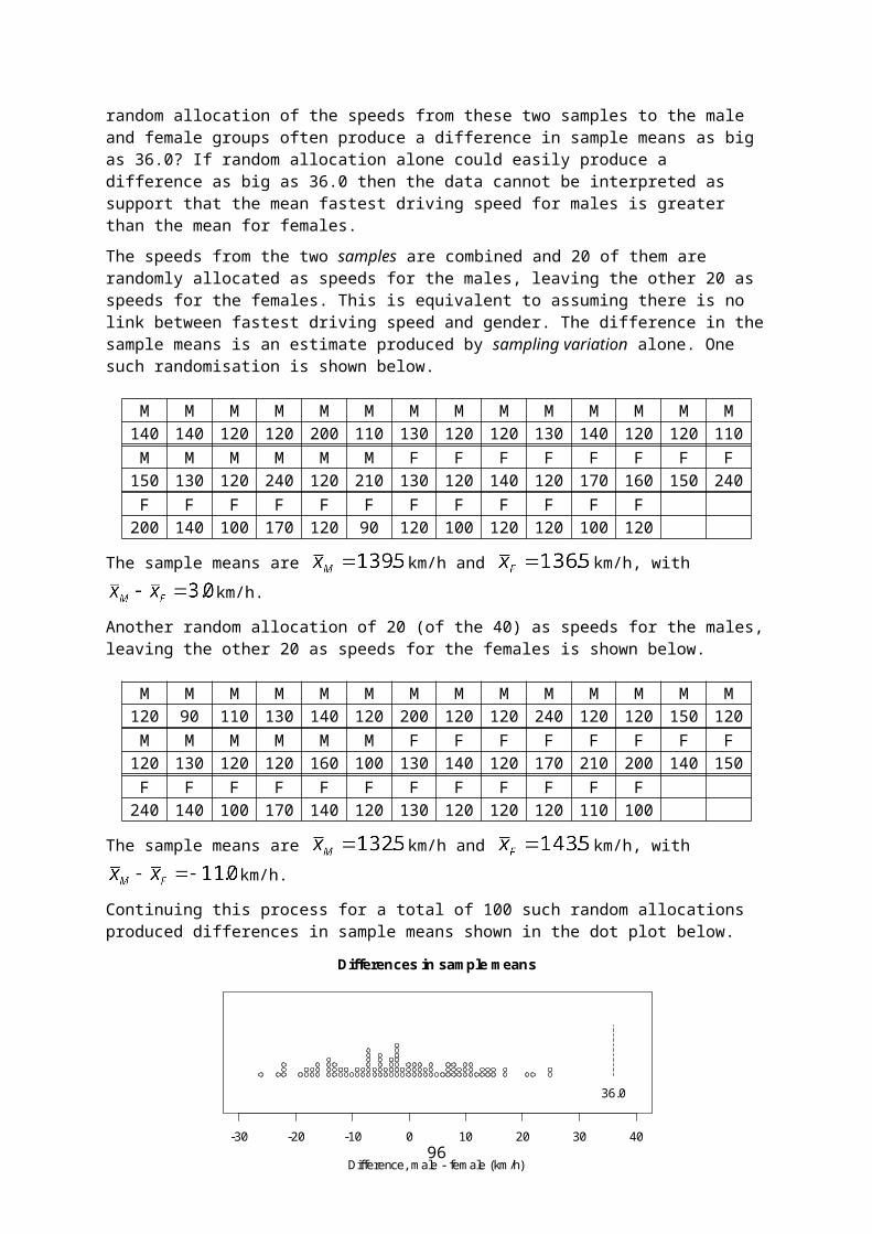
If about 5% of the estimates produced by random allocation alone are at least as far from zero as the observed estimate then the data provide some evidence of a link between the two variables.

If about 10% of the estimates produced by random allocation alone are at least as far from zero as the observed estimate then the data provide weak evidence of a link between the two variables.

If more than about 12% of the estimates produced by random allocation alone are at least as far from zero as the observed estimate then the data provide no evidence of a link between the two variables.

Two examples of using resampling using randomisation are provided in the description of randomisation. These examples include a conclusion about the strength of evidence the data provide for a link between the two variables.

See: randomisation, resampling


Strip graphA graph for displaying the distribution of a category variable or a whole-number variable that uses parts of a rectangular strip to represent the frequencies for each category or value.

Example

A student collected data on the colour of cars that drove past her house and displayed the results on the strip graph below.

Colours of cars

Alternative: segmented bar graph


Summary statisticsNumbers calculated from numerical data that are used to summarise the data. The statistics will usually include at least one measure of centre and at least one measure of spread.

Alternatives: descriptive statistics, numerical summary

See: sample statistics


96

red grey/silver gold green blue white

SurveyA systematic collection of data taken by questioning a sample of people taken from a population in order to estimate a population parameter.

Alternative: sample survey

See: poll

Curriculum achievement objectives referencesStatistical investigation: Levels 5, (6), 7, 8Statistical literacy: Levels 7, 8

SymmetryA property of a distribution of a numerical variable when the values below the centre of the distribution are distributed in the same way as the values above the centre.

Many theoretical distributions are not symmetrical. For example, all Poisson distributions are not symmetrical.

Frequency distributions from experiments or samples (i.e., experimental distributions or sample distributions are unlikely to show perfect symmetry. This may be because the distribution of the population from which the values came is not symmetrical. Alternatively, if the distribution of the population from which the values came is symmetrical, then the presence of sampling variation will cause the frequency distribution to not be perfectly symmetrical.

Example (A symmetrical theoretical discrete distribution)

The bar graph displays the probability function of the binomial distribution with n = 10 and π = 0.5. The graph is symmetrical.


97

0 1 2 3 4 5 6 7 8 9 10

Pro

babi

lity

0.00

0.05

0.10

0.15

0.20

0.25


Systematic samplingA method of sampling from a list of the population so that the sample is made up of every kth member on the list, after randomly selecting a starting point from 1 to k.

Example

Consider choosing a systematic sample of 20 members from a population list numbered from 1 to 836.

To find k, divide 836 by 20 to get 41.8.

Rounding gives k = 42.

Randomly select a number from 1 to 42, say 18.

Start at the person numbered 18 and then choose every 42nd member of the list.

The sample is made up of those numbered:18, 60, 102, 144, 186, 228, 270, 312, 354, 396, 438, 480, 522, 564, 606, 648, 690, 732, 774, 816

Sometimes rounding may cause the sample size to be one more or one less than the desired size.


Tally chartA table used to record values for a variable in a data set, by hand, often as the values are collected. One tally mark is used for each occurrence of a value. Tally marks are usually grouped in sets of five, to aid the counting of the frequency for each value.

A tally chart provides an immediate visual form of the distribution.

Example

The number of days in a week that rain fell in Grey Lynn, Auckland, from Monday 2 January 2006 to Sunday 31 December 2006 is recorded in the tally chart below.

Number of days with rain Number of weeks0 ||1 ||||2 ||||3 ||||4 |||| |||| |||| ||||5 |||| |6 |||| |7 ||||

98

The tally chart can then be re-drawn as the following frequency table.


Total 52


Theoretical distributionA model for the variation in the values of a variable based on defining the probabilities of values (or intervals of values) of a variable.

Example

The Poisson distribution is a theoretical distribution.

Curriculum achievement objectives referencesStatistical investigation: (Level 8)Probability: Levels 5, 6, 7, (8)

Time-series dataA data set gathered over time. For one object, such as climate in Rolleston, Canterbury, the values of a variable (or several variables) are obtained at successive times. Usually there are equal intervals between the successive times.

Example

The maximum temperature, rainfall, maximum atmospheric pressure and maximum wind gust speed in Rolleston, recorded daily.

Note: At Level Eight a common approach to modelling time-series data considers the data to have four components; trend component, cyclical component, seasonal component and irregular component.

See: additive model (for time-series data)

Curriculum achievement objectives referencesStatistical investigation: Levels 3, 4, (5), (6), (7), 8

99

TreatmentIn an experiment, the value of the explanatory variable that is chosen by the researcher to be given to each individual in a group.

See: experiment

Curriculum achievement objectives referencesStatistical investigation: Levels (7), (8)Statistical literacy: (Level 8)

Tree diagramA diagram used to represent the possible outcomes in a probability activity that has more than one stage.

From a single starting point, a branch is drawn to represent the outcomes of the first stage. From the end of each branch, a second branch is drawn to represent the outcomes of the second stage, and so on. From the starting point, each path through the tree represents an outcome of the whole activity.

A tree diagram can be a useful tool for obtaining a systematic list all of the possible outcomes of a probability activity that involves two or three stages (see Example 1). The use of tree diagrams is usually restricted to two-stage or three-stage probability activities because they become too complicated when the total number of outcomes is large.

If the outcomes at each stage are not equally likely to occur then, for each stage, the probability of each outcome for each stage is written on a branch.

Example 1 (Outcomes only, no probabilities on branches)

In a game of tennis one player from School A is to play one player from School B. School A has 3 players to choose from (C, D and E) and School B has 2 players to choose from (F and G). If each player has an equal chance of being selected to play for their school, list all of the different possible combinations of games.

100

School A School B GameC plays F

C plays G

D plays F

D plays G

E plays F

E plays G

C

D

E

F

F

F

G

G

G

Example 2 (Independent stages, probabilities on branches)

In a game of tennis one player from School A is to play one player from School B. School A has 3 players to choose from (C, D and E) and School B has 2 players to choose from (F and G). For School A, the probabilities of C, D or E being selected are 0.6, 0.3 and 0.1 respectively. For school B, the probabilities of F or G being selected are 0.7 and 0.3 respectively. List all of the different possible combinations of games with their probabilities. Assume that choosing a player from School A is independent of choosing a player from School B.

Example 3 (Conditional stages, probabilities on branches)

A jar contains 10 balls, 7 are blue and 3 are red. A ball is randomly taken from the jar and its colour is noted. The ball is not placed back in the jar and a second ball is randomly taken from the jar. List all of the different possible outcomes of this probability activity with their probabilities.


101

C

D

E

F

G

F

G

F

G

C plays F

C plays G

D plays F

D plays G

E plays F

E plays G

0.6

0.3

0.1

School A School B Game Probability0.42

0.18

0.21

0.09

0.07

0.03

0.7

0.3

0.7

0.3

0.7

0.3

B1

R1

Draw 1 Draw 2 Outcome Probability

B2 | B1

R2 | B1

B2 | R1

R2 | R1

B1 and B2

B1 and R2

R1 and B2

R1 and R2

7/10

3/10

6/9

3/9

7/9

2/9

42/90 = 14/30

21/90 = 7/30

21/90 = 7/30

6/90 = 2/30

TrendA general tendency among variables in a data set; usually between pairs of variables.

For two numerical variables, as values of one variable increase the trend is any general tendency of the change in the values of the other variable. See Example 1 below.

For two category variables, both of which have a natural ordering of their categories, as transitions are made from the lowest to the highest category, the trend is any general tendency of the changes in the categories of the other variable. See Example 2 below.

For a category variable that has a natural ordering of its categories and a numerical variable, as transitions are made from the lowest to the highest category for the category variable the trend is any general tendency of the changes in the values of the numerical variable. See Example 3 below.

For time-series data the trend is any general tendency to change with time. See Example 4 below.

Example 1 (Two numerical variables)

Data were selected for 86 New Zealand school students from the CensusAtSchool website. The scatter plot below displays the data for their height and right foot length, both in centimetres.

As the length of the right foot increases there is a general tendency for height to increase. The trend is that, generally, an increase is right foot length is associated with an increase in height.

Example 2 (Two category variables, with a natural ordering of categories)

Data were selected for 86 New Zealand school students from the CensusAtSchool website. Two of the variables were their year level (5 or 6, 7 or 8, 9 or 10) and their usual level of lunchtime activity (Sit or stand, Walk, Run). The data are displayed in the two-way table and bar graph below. The table shows frequencies for each cell, as well as row proportions for each of the three groups of year levels.

102

15 20 25 30 35

120

130

140

150

160

170

180

Height against right foot length

Right foot length (cm)

Hei

ght (

cm)

Lunchtime activityYear level Sit or stand Walk Run Total5 or 6 1 2 23 26

(3.8%) (7.7%) (88.5%)7 or 8 1 4 16 21

(4.8%) (19.0%) (76.2%)9 or 10 18 9 12 39

(46.2%) (23.1%) (30.8%)Total 20 15 51 86

As we move from year levels 5 or 6 to year levels 9 or 10 there is a general tendency for the proportion running during lunchtime to decrease and the proportion sitting or standing to increase. The trend is that for higher year levels, generally, there is an increase in less vigorous forms of lunchtime activity.

Example 3 (One numerical variable and one category variable with a natural ordering of categories)

Data were selected for 86 New Zealand school students from the CensusAtSchool website. The dot plot below displays the data for their heights, in centimetres, for three groups of year levels.

103

120 130 140 150 160 170 180

5 or

67

or 8

9 or

10

Height for year levels

Height (cm)

Yea

r le

vel

5 or 6 7 or 8 9 or 10

Lunchtime activity by year level

Year level

Pro

port

ion

0.0

0.2

0.4

0.6

0.8

Sit/standWalkRun

As we move from year levels 5 or 6 to year levels 9 or 10 there is a general tendency for height to increase. The trend is for students at higher year levels to be taller, in general.

Example 4 (Time-series data)

Statistics New Zealand’s Economic Survey of Manufacturing provided the following data on actual operating income for the manufacturing sector in New Zealand for each quarter from September 2002 to September 2008. Note that M, J, S and D indicate quarter years ending in March, June, September and December respectively.

Over time there is a general tendency for the operating income to increase. The trend is that as time goes by, generally, there is an increase in operating income.

Curriculum achievement objectives referencesStatistical investigation: Levels 3, 4, 5, 6, (7), (8)

Trend component (for time-series data)The general tendency in time-series data. The trend component is the slow variation in the time series over a long period of time, relative to the interval between the successive times.



Two-way tableA table in which the rows represent the categories for one category variable, the columns represent the categories of a second category variable and each cell displays the frequency (or proportion) resulting for that row and column combination for the two variables.

104

15

16

17

18

19

20

21

22


Quarter

Ope

ratin

g in

com

e ($

billio

ns)

S-0

2D

-02

M-0

3J-

03S

-03

D-0

3M

-04

J-04

S-0

4D

-04

M-0

5J-

05S

-05

D-0

5M

-06

J-06

S-0

6D

-06

M-0

7J-

07S

-07

D-0

7M

-08

J-08

S-0

8

Example

Data were collected from answers to an online questionnaire from 727 students enrolled in an introductory Statistics course at the University of Auckland. Two of the variables of interest are the gender of the student and the course in which they which they were enrolled (STATS 101, STATS 102 or STATS 108). The following two-way table was formed by counting the number of students falling into each combination of categories of the two variables.

Course101 102 108 Total

GenderFemale 218 50 157 425Male 141 18 143 302Total 359 68 300 727

Alternative: contingency table


Upper quartileSee: quartiles


VariabilityThe tendency for a property to have different values for different individuals or to have different values at different times.

Curriculum achievement objectives referencesStatistical investigation: Levels (1), (2), (3), (4), (5), (6), 7, (8)Probability: Levels (1), (2), (3), (4), (5), (6), (7), (8)

VariableA property that may have different values for different individuals or that may have different values at different times.

Curriculum achievement objectives referencesStatistical investigation: Levels 4, 5, 6, 7, (8)Probability: Levels (7), 8

105

VarianceA measure of spread for a distribution of a numerical variable that determines the degree to which the values differ from the mean. If many values are close to the mean then the variance is small and if many values are far from the mean then the variance is large.

It is calculated by the average of the squares of the deviations of the values from their mean.

The variance can be influenced by unusually large or unusually small values.

The positive square root of the variance is equal to the standard deviation.

It is recommended that a calculator or software is used to calculate the variance. On a calculator the square of the standard deviation will give the variance.

See: measure of spread, sample variance, standard deviation


Variance (of a discrete random variable)A measure of spread for a distribution of a random variable that determines the degree to which the values of a random variable differ from the expected value.

The variance of random variable X is often written as Var(X) or σ2 or .

For a discrete random variable the variance is calculated by summing the product of the square of the difference between the value of the random variable and the expected value, and the associated probability of the value of the random variable, taken over all of the values of the random variable.

In symbols, Var(X) =

An equivalent formula is, Var(X) = E(X2) – [E(X)]2

The square root of the variance is equal to the standard deviation.

Example


x 0 1 2 3P(X = x) 0.1 0.2 0.4 0.3

Using Var(X) =

µ = 0 x 0.1 + 1 x 0.2 + 2 x 0.4 + 3 x 0.3

= 1.9

Var(X) = (0 – 1.9)2 + (1 – 1.9)2 + (2 – 1.9)2 + (3 – 1.9)2

= 0.89

106

Using Var(X) = E(X2) – [E(X)]2

E(X) = 0 x 0.1 + 1 x 0.2 + 2 x 0.4 + 3 x 0.3

= 1.9

E(X2) = 02 × 0.1 + 12 × 0.2 + 22 × 0.4 + 32 × 0.3

= 4.5

Var(X) = 4.5 – 1.92

= 0.89

See: population variance, variance


VariationThe differences seen in the values of a property for different individuals or at different times.

Curriculum achievement objectives referencesStatistical investigation: Levels 4, 5, 6Probability: Levels (1), (2), (3), 4, 5, (6), (7), (8)

Whole-number dataData in which the values result from counting, or from measuring with the values rounded to a whole number.

Example 1 (Values from counting)

The number of students absent from each class in a primary school on a particular day.

Example 2 (Values from measuring)

The heights of a class of Year 9 students recorded to the nearest centimetre.

See: numerical data, quantitative data

Curriculum achievement objectives referencesStatistical investigation: Levels 2, 3, (4), (5), (6), (7), (8)

107

Whole-number variableA property that may have different values for different individuals and for which these values result from counting, or from measuring with the values rounded to a whole number.

Example 1 (Values from counting)

The number of students absent from each class in a primary school on a particular day.

Example 2 (Values from measuring)

The heights of a class of Year 9 students recorded to the nearest centimetre.

See: numerical variable, quantitative variable


108

trend component (for time-series data) - home - senior...

Documents