Tree-Structured Indexes

Lecture 17R & G Chapter 9

“If I had eight hours to chop down a tree, I'd spend six sharpening my ax.”

Abraham Lincoln

Administrivia

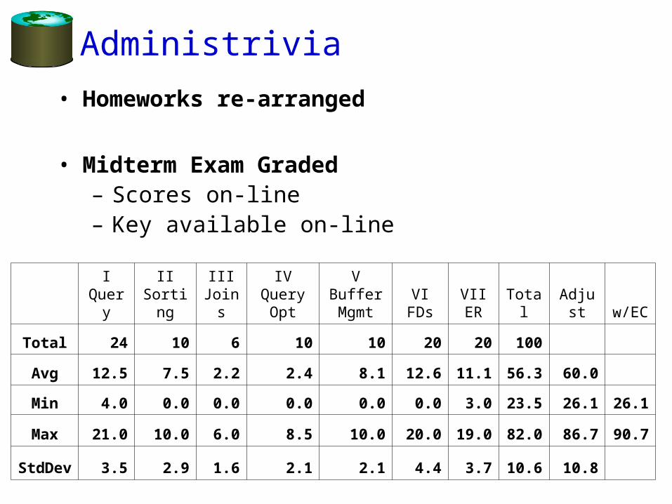
• Homeworks re-arranged

• Midterm Exam Graded– Scores on-line– Key available on-line

IQuery

IISorting

IIIJoins

IVQuery

Opt

VBuffer Mgmt

VIFDs

VIIER Total Adjust w/EC

Total 24 10 6 10 10 20 20 100

Avg 12.5 7.5 2.2 2.4 8.1 12.6 11.1 56.3 60.0

Min 4.0 0.0 0.0 0.0 0.0 0.0 3.0 23.5 26.1 26.1

Max 21.0 10.0 6.0 8.5 10.0 20.0 19.0 82.0 86.7 90.7

StdDev 3.5 2.9 1.6 2.1 2.1 4.4 3.7 10.6 10.8

Review• Last week:

– How Internet Apps use Databases– How to access Databases from Programs– How to extend Databases with Programs

• This week:– Tree Indexes (HW4 or 5?)– Hash Indexes

• Next week:– Transactions– Concurrency Control

Today: B-Tree Indexes

• Discussed costs/benefits in lecture 5

• Today more detail:– ISAM, an old fashioned Tree Index– B-Trees, most common DBMS tree index

Introduction• Recall: 3 alternatives for data entries k*:

• Data record with key value k• <k, rid of data record with search key value k>• <k, list of rids of data records with search key

k>• Choice is orthogonal to the indexing

technique used to locate data entries k*.• Tree-structured indexing techniques support

both range searches and equality searches.• ISAM: static structure; B+ tree: dynamic,

adjusts gracefully under inserts and deletes.• ISAM = ???

Indexed Sequential Access Method

A Note of Caution

• ISAM is an old-fashioned idea– B+-trees are usually better, as we’ll see

• Though not always

• But, it’s a good place to start– Simpler than B+-tree, but many of the same ideas

• Upshot– Don’t brag about being an ISAM expert on your

resume– Do understand how they work, tradeoffs with B+-

trees

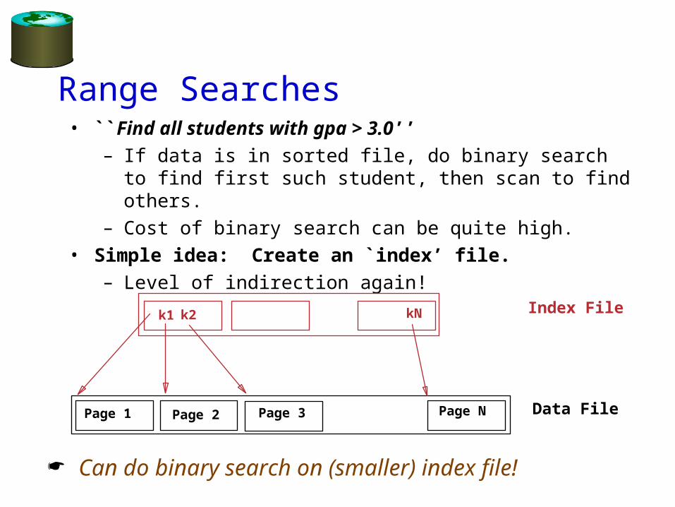
Range Searches• ``Find all students with gpa > 3.0’’

– If data is in sorted file, do binary search to find first such student, then scan to find others.

– Cost of binary search can be quite high.• Simple idea: Create an `index’ file.

– Level of indirection again!

Can do binary search on (smaller) index file!

Page 1 Page 2 Page NPage 3 Data File

k2 kNk1 Index File

ISAM

• Index file may still be quite large. But we can apply the idea repeatedly!

Leaf pages contain data entries.

P0

K1 P

1K 2 P

2K m

P m

index entry

Non-leaf

Pages

Pages

Overflow page

Primary pages

Leaf

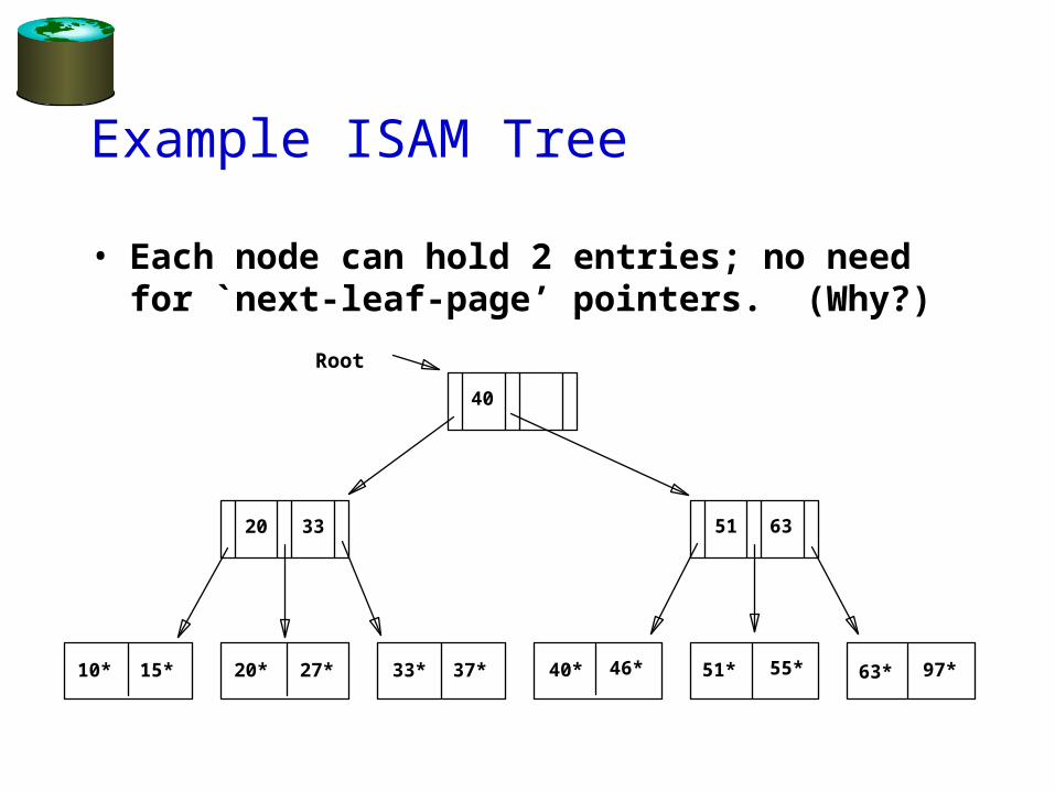
Example ISAM Tree

• Each node can hold 2 entries; no need for `next-leaf-page’ pointers. (Why?)

10* 15* 20* 27* 33* 37* 40* 46* 51* 55* 63* 97*

20 33 51 63

40

Root

Comments on ISAM

• File creation: Leaf (data) pages allocated sequentially, sorted by search key. Then index pages allocated. Then space for overflow pages.

• Index entries: <search key value, page id>; they `direct’ search for data entries, which are in leaf pages.

• Search: Start at root; use key comparisons to go to leaf. Cost log F N ; F = # entries/index pg, N = # leaf pgs

• Insert: Find leaf where data entry belongs, put it there.(Could be on an overflow page).

• Delete: Find and remove from leaf; if empty overflow page, de-allocate.

Static tree structure: inserts/deletes affect only leaf pages.

Data Pages

Index Pages

Overflow pages

Example ISAM Tree

• Each node can hold 2 entries; no need for `next-leaf-page’ pointers. (Why?)

10* 15* 20* 27* 33* 37* 40* 46* 51* 55* 63* 97*

20 33 51 63

40

Root

After Inserting 23*, 48*, 41*, 42* ...

10* 15* 20* 27* 33* 37* 40* 46* 51* 55* 63* 97*

20 33 51 63

40

Root

23* 48* 41*

42*

Overflow

Pages

Leaf

Index

Pages

Pages

Primary

... then Deleting 42*, 51*, 97*

Note that 51 appears in index levels, but 51* not in leaf!

10* 15* 20* 27* 33* 37* 40* 46* 55* 63*

20 33 51 63

40

Root

23* 48* 41*

ISAM ---- Issues?

• Pros– ????

• Cons– ????

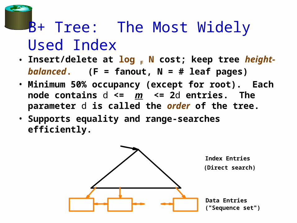
B+ Tree: The Most Widely Used Index

• Insert/delete at log F N cost; keep tree height-balanced. (F = fanout, N = # leaf pages)

• Minimum 50% occupancy (except for root). Each node contains d <= m <= 2d entries. The parameter d is called the order of the tree.

• Supports equality and range-searches efficiently.

Index Entries

Data Entries("Sequence set")

(Direct search)

Example B+ Tree

• Search begins at root, and key comparisons direct it to a leaf (as in ISAM).

• Search for 5*, 15*, all data entries >= 24* ...

Based on the search for 15*, we know it is not in the tree!

Root

17 24 30

2* 3* 5* 7* 14* 16* 19* 20* 22* 24* 27* 29* 33* 34* 38* 39*

13

B+ Trees in Practice

• Typical order: 100. Typical fill-factor: 67%.– average fanout = 133

• Typical capacities:– Height 4: 1334 = 312,900,700 records– Height 3: 1333 = 2,352,637 records

• Can often hold top levels in buffer pool:– Level 1 = 1 page = 8 Kbytes– Level 2 = 133 pages = 1 Mbyte– Level 3 = 17,689 pages = 133 MBytes

Inserting a Data Entry into a B+ Tree• Find correct leaf L. • Put data entry onto L.

– If L has enough space, done!– Else, must split L (into L and a new node L2)

• Redistribute entries evenly, copy up middle key.• Insert index entry pointing to L2 into parent of L.

• This can happen recursively– To split index node, redistribute entries evenly, but

push up middle key. (Contrast with leaf splits.)• Splits “grow” tree; root split increases height.

– Tree growth: gets wider or one level taller at top.

Example B+ Tree - Inserting 8*

Root

17 24 30

2* 3* 5* 7* 14* 16* 19* 20* 22* 24* 27* 29* 33* 34* 38* 39*

13

Example B+ Tree - Inserting 8*

Notice that root was split, leading to increase in height.

In this example, we can avoid split by re-distributing entries; however, this is usually not done in practice.

2* 3*

Root

17

24 30

14* 16* 19*20* 22* 24* 27*29* 33* 34* 38* 39*

135

7*5* 8*

Inserting 8* into Example B+ Tree

• Observe how minimum occupancy is guaranteed in both leaf and index pg splits.

• Note difference between copy-up and push-up; be sure you understand the reasons for this.

2* 3* 5* 7* 8*

5

Entry to be inserted in parent node.(Note that 5 iscontinues to appear in the leaf.)

s copied up and

appears once in the index. Contrast

5 24 30

17

13

Entry to be inserted in parent node.(Note that 17 is pushed up and only

this with a leaf split.)

…

…

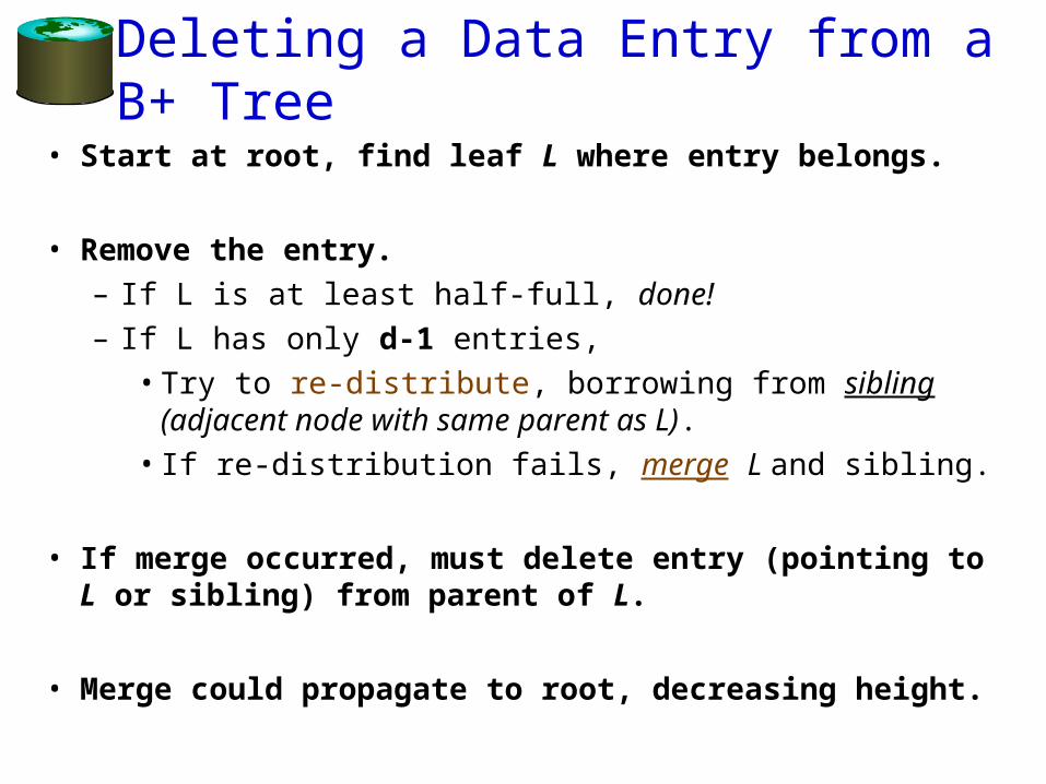
Deleting a Data Entry from a B+ Tree

• Start at root, find leaf L where entry belongs.

• Remove the entry.– If L is at least half-full, done! – If L has only d-1 entries,

• Try to re-distribute, borrowing from sibling (adjacent node with same parent as L).

• If re-distribution fails, merge L and sibling.

• If merge occurred, must delete entry (pointing to L or sibling) from parent of L.

• Merge could propagate to root, decreasing height.

Example Tree (including 8*) Delete 19* and 20* ...

• Deleting 19* is easy.

2* 3*

Root

17

24 30

14* 16* 19*20* 22* 24* 27*29* 33* 34* 38* 39*

135

7*5* 8*

Example Tree (including 8*) Delete 19* and 20* ...

• Deleting 19* is easy.• Deleting 20* is done with re-distribution.

Notice how middle key is copied up.

2* 3*

Root

17

30

14* 16* 33* 34* 38* 39*

135

7*5* 8* 22*24*

27

27* 29*

... And Then Deleting 24*• Must merge.• Observe `toss’ of

index entry (on right), and `pull down’ of index entry (below).

30

22* 27* 29* 33* 34* 38* 39*

2* 3* 7* 14* 16* 22* 27* 29* 33* 34* 38* 39*5* 8*

Root30135 17

Example of Non-leaf Re-distribution

• Tree is shown below during deletion of 24*. (What could be a possible initial tree?)

• In contrast to previous example, can re-distribute entry from left child of root to right child.

Root

135 17 20

22

30

14* 16* 17* 18* 20* 33* 34* 38* 39*22* 27* 29*21*7*5* 8*3*2*

After Re-distribution• Intuitively, entries are re-distributed by

`pushing through’ the splitting entry in the parent node.

• It suffices to re-distribute index entry with key 20; we’ve re-distributed 17 as well for illustration.

14* 16* 33* 34* 38* 39*22* 27* 29*17* 18* 20* 21*7*5* 8*2* 3*

Root

135

17

3020 22

Prefix Key Compression• Important to increase fan-out. (Why?)• Key values in index entries only `direct traffic’;

can often compress them.– E.g., If we have adjacent index entries with search

key values Dannon Yogurt, David Smith and Devarakonda Murthy, we can abbreviate David Smith to Dav. (The other keys can be compressed too ...)

• Is this correct? Not quite! What if there is a data entry Davey Jones? (Can only compress David Smith to Davi)

• In general, while compressing, must leave each index entry greater than every key value (in any subtree) to its left.

• Insert/delete must be suitably modified.

Bulk Loading of a B+ Tree• If we have a large collection of records, and

we want to create a B+ tree on some field, doing so by repeatedly inserting records is very slow.– Also leads to minimal leaf utilization --- why?

• Bulk Loading can be done much more efficiently.

• Initialization: Sort all data entries, insert pointer to first (leaf) page in a new (root) page.

3* 4* 6* 9* 10* 11* 12* 13* 20* 22* 23* 31* 35* 36* 38* 41* 44*

Sorted pages of data entries; not yet in B+ treeRoot

Bulk Loading (Contd.)

• Index entries for leaf pages always entered into right-most index page just above leaf level. When this fills up, it splits. (Split may go up right-most path to the root.)

• Much faster than repeated inserts, especially when one considers locking!

3* 4* 6* 9* 10*11* 12*13* 20*22* 23* 31* 35*36* 38*41* 44*

Root

Data entry pages

not yet in B+ tree3523126

10 20

3* 4* 6* 9* 10* 11* 12*13* 20*22* 23* 31* 35*36* 38*41* 44*

6

Root

10

12 23

20

35

38

not yet in B+ treeData entry pages

Summary of Bulk Loading

• Option 1: multiple inserts.– Slow.– Does not give sequential storage of leaves.

• Option 2: Bulk Loading – Has advantages for concurrency control.– Fewer I/Os during build.– Leaves will be stored sequentially (and

linked, of course).– Can control “fill factor” on pages.

A Note on `Order’

• Order (d) concept replaced by physical space criterion in practice (`at least half-full’).– Index pages can typically hold many more entries than

leaf pages.– Variable sized records and search keys mean different

nodes will contain different numbers of entries.– Even with fixed length fields, multiple records with the

same search key value (duplicates) can lead to variable-sized data entries (if we use Alternative (3)).

• Many real systems are even sloppier than this --- only reclaim space when a page is completely empty.

Summary• Tree-structured indexes are ideal for range-

searches, also good for equality searches.• ISAM is a static structure.

– Only leaf pages modified; overflow pages needed.– Overflow chains can degrade performance unless

size of data set and data distribution stay constant.• B+ tree is a dynamic structure.

– Inserts/deletes leave tree height-balanced; log F N cost.

– High fanout (F) means depth rarely more than 3 or 4.– Almost always better than maintaining a sorted file.

Summary (Contd.)

– Typically, 67% occupancy on average.– Usually preferable to ISAM, adjusts to growth gracefully.– If data entries are data records, splits can change rids!

• Key compression increases fanout, reduces height.• Bulk loading can be much faster than repeated

inserts for creating a B+ tree on a large data set.• Most widely used index in database management

systems because of its versatility. One of the most optimized components of a DBMS.