treatment of singularities in the method of fundamental solutions for two-dimensional helmholtz-type...
TRANSCRIPT

Applied Mathematical Modelling 34 (2010) 1615–1633
Contents lists available at ScienceDirect
Applied Mathematical Modelling
journal homepage: www.elsevier .com/locate /apm
Treatment of singularities in the method of fundamental solutionsfor two-dimensional Helmholtz-type equations
Liviu MarinInstitute of Solid Mechanics, Romanian Academy, 15 Constantin Mille, Sector 1, P.O. Box 1-863, 010141 Bucharest, Romania
a r t i c l e i n f o
Article history:Received 13 February 2009Received in revised form 30 August 2009Accepted 2 September 2009Available online 11 September 2009
Keywords:Helmholtz-type equationsSingular problemsSingularity subtraction technique (SST)Method of fundamental solutions (MFS)
0307-904X/$ - see front matter � 2009 Elsevier Incdoi:10.1016/j.apm.2009.09.009
E-mail addresses: [email protected], liviu@
a b s t r a c t
We investigate a meshless method for the accurate and non-oscillatory solution of prob-lems associated with two-dimensional Helmholtz-type equations in the presence ofboundary singularities. The governing equation and boundary conditions are approximatedby the method of fundamental solutions (MFS). It is well known that the existence ofboundary singularities affects adversely the accuracy and convergence of standard numer-ical methods. The solutions to such problems and/or their corresponding derivatives mayhave unbounded values in the vicinity of the singularity. This difficulty is overcome by sub-tracting from the original MFS solution the corresponding singular functions, without anappreciable increase in the computational effort and at the same time keeping the sameMFS approximation. Four examples for both the Helmholtz and the modified Helmholtzequations are carefully investigated and the numerical results presented show an excellentperformance of the approach developed.
� 2009 Elsevier Inc. All rights reserved.
1. Introduction
In many engineering problems governed by elliptic partial differential equations, boundary singularities arise when thereare sharp re-entrant corners in the boundary, the boundary conditions change abruptly, or there are discontinuities in thematerial properties. It is well known that these situations give rise to singularities of various types and, as a consequence,the solutions to such problems and/or their corresponding derivatives may have unbounded values in the vicinity of the sin-gularity. Singularities are known to affect adversely the accuracy and convergence of standard numerical methods, such asfinite element (FEM), boundary element (BEM), finite-difference (FDM), spectral and meshless/meshfree methods. When thecomputed function is bounded, but has a branch point at the corner, the difficulty is not serious. Grid refinement and higher-order discretizations are common strategies aimed at improving the convergence rate and accuracy of the above-mentionedstandard methods, see e.g. Apel et al. [1] or Apel and Nicaise [2]. If, however, the form of the singularity is taken into accountand is properly incorporated into the numerical scheme then a more effective method may be constructed.
Helmholtz-type equations arise naturally in many physical applications related to wave propagation and vibration phe-nomena. They are often used to describe the vibration of a structure [3,4], the acoustic cavity problem [5,6], the radiationwave [7,8], the scattering of a wave [9,10] and the heat conduction in fins [11,12]. The knowledge of the associated boundaryconditions on the entire boundary of the solution domain gives rise to problems for Helmholtz-type equations which havebeen extensively studied in the literature [13,14].
There are important studies regarding the numerical treatment of singularities occurring in Helmholtz-type equations.Time-harmonic waves in a membrane which contains one or more fixed edge stringers or cracks have been investigatedby Chen et al. [4] who have employed the dual BEM in order to obtain an efficient solution of the Helmholtz equation in
. All rights reserved.
imsar.bu.edu.ro
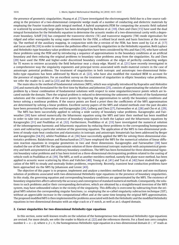
1616 L. Marin / Applied Mathematical Modelling 34 (2010) 1615–1633
the presence of geometric singularities. Huang et al. [7] have investigated the electromagnetic field due to a line source radi-ating in the presence of a two-dimensional composite wedge made of a number of conducting and dielectric materials byemploying the Fourier transform path integral method. A hybrid asymptotic/FEM for computing the acoustic field radiatedor scattered by acoustically large objects has been developed by Barbone et al. [10]. Chen and Chen [15] have used the dualintegral formulation for the Helmholtz equation to determine the acoustic modes of a two-dimensional cavity with a degen-erate boundary. Schiff [16] has computed the transverse electric (TE) and transverse magnetic (TM) mode eigenvalues forridged and other waveguides by using super-elements for the FEM, a refined local mesh and basis functions at the cornertip. The method of the auxiliary mapping, in conjunction with the p-version of the FEM, has been used by Cai et al. [17]and Lucas and Oh [18] in order to remove the pollution effect caused by singularities in the Helmholtz equation. Both Laplaceand Helmholtz-type boundary value problems with singularities have been considered by Wu and Han [19], who have solvedthese problems using the FEM and by introducing a sequence of approximations to the boundary conditions at an artificialboundary and then reducing the original problems to boundary value problems away from the singularities. Xu and Chen[20] have used the FDM and higher-order discretized boundary conditions at the edges of perfectly conducting wedgesfor TE waves to retrieve accurately the field behaviour near a sharp edge. Mantic et al. [21] have recently investigated ina comprehensive way the singularity exponents and principal terms associated with multi-material corners in the case ofanisotropic potential problems. The treatment of singularities in both isotropic and anisotropic two-dimensional Helm-holtz-type equations has been addressed by Marin et al. [22], who have also modified the standard BEM to account forthe presence of singularities. For an excellent survey on the treatment of singularities in elliptic boundary value problems,we refer the reader to Li and Lu [23] and the references therein.
The main idea in the method of fundamental solutions (MFS), which was originally introduced by Kupradze and Aleksidze[24] and numerically formulated for the first time by Mathon and Johnston [25], consists of approximating the solution of theproblem by a linear combination of fundamental solutions with respect to some singularities/source points which are lo-cated outside the domain. Then the original problem is reduced to determining the unknown coefficients of the fundamentalsolutions and the coordinates of the source points by requiring the approximation to satisfy the boundary conditions andhence solving a nonlinear problem. If the source points are fixed a priori then the coefficients of the MFS approximationare determined by solving a linear problem. Excellent survey papers of the MFS and related methods over the past decadeshave been presented by Fairweather and Karageorghis [26], Golberg and Chen [27], Fairweather et al. [28] and Cho et al. [29].
The MFS has been successfully applied to solving a wide variety of boundary value problems. Karageorghis and Fair-weather [30] have solved numerically the biharmonic equation using the MFS and later their method has been modifiedin order to take into account the presence of boundary singularities in both the Laplace and the biharmonic equations byKarageorghis [31] and Poullikkas et al. [32]. Furthermore, Poullikkas et al. [33] have investigated the numerical solutionof the inhomogeneous harmonic and biharmonic equations by reducing these problems to the corresponding homogeneouscases and subtracting a particular solution of the governing equation. The application of the MFS to two-dimensional prob-lems of steady-state heat conduction and elastostatics in isotropic and anisotropic bimaterials has been addressed by Bergerand Karageorghis [34,35], whilst Poullikkas et al. [36] have successfully applied the MFS for solving three-dimensional elas-tostatics problems. Balakrishnan and Ramachandran [37] have employed the MFS for the numerical solution of linear diffu-sion reaction equations in irregular geometries in two and three dimensions. Karageorghis and Fairweather [38] havestudied the use of the MFS for the approximate solution of three-dimensional isotropic materials with axisymmetrical geom-etry and both axisymmetrical and arbitrary boundary conditions. The MFS has been formulated for three-dimensional Signo-rini boundary value problems and it has been tested on a three-dimensional electropainting problem related to the coating ofvehicle roofs in Poullikkas et al. [39]. The MFS, as well as another meshless method, namely the plane wave method, has beenapplied to acoustic wave scattering by Alves and Valtchev [40]. Young et al. [41] and Tsai et al. [42] have studied the appli-cation of the MFS to steady and unsteady Stokes problems, respectively. Recently, transient heat conduction problems havebeen approached via the MFS by Johansson and Lesnic [43].
The objective of this paper is to propose, implement and analyse a meshless method for the accurate and non-oscillatorysolution of problems associated with two-dimensional Helmholtz-type equations in the presence of boundary singularities.In this study, the governing equation and corresponding boundary conditions are approximated by the MFS. The existence ofboundary singularities affects adversely the accuracy and convergence of standard numerical methods. Consequently, the solu-tions to such problems and/or their corresponding derivatives, which are obtained by a straightforward inversion of the MFSsystem, may have unbounded values in the vicinity of the singularity. This difficulty is overcome by subtracting from the ori-ginal MFS solution the corresponding singular functions, i.e. employing the so-called singularity subtraction technique (SST),without an appreciable increase in the computational effort and at the same time keeping the original MFS approximation.The proposed modified MFS is then implemented for problems associated with both the Helmholtz and the modified Helmholtzequations in two-dimensional domains with an edge crack or a V-notch, as well as an L-shaped domain.
2. Corner singularities for two-dimensional Helmholtz-type equations
In this section, some well-known results on the solution of the homogeneous two-dimensional Helmholtz-type equationsare revised. For more details, we refer the reader to Marin et al. [22] and the references therein. For a fixed non-zero complexnumber k ¼ aþ ib, where a; b 2 R, the homogeneous Helmholtz-type equation in a two-dimensional domain X � R2 reads as

L. Marin / Applied Mathematical Modelling 34 (2010) 1615–1633 1617
DuðxÞ þ k2uðxÞ � @2uðxÞ@x2
1
þ @2uðxÞ@x2
2
þ k2uðxÞ ¼ 0; x ¼ ðx1; x2Þ 2 X: ð1Þ
Let the polar coordinate system ðr; hÞ be defined in the usual way with respect to the Cartesian coordinatesðx1; x2Þ ¼ ðr cos h; r sin hÞ. If we assume that the solution of Eq. (1) in the domain X can be written using the separation ofvariables with respect to the polar coordinates ðr; hÞ, where r > 0, then the general solution of the Helmholtz-type equation(1) can be written as
uðr; hÞ ¼ c1JkðkrÞ þ c2NkðkrÞ½ � a cosðkhÞ þ b sinðkhÞ½ �: ð2Þ
Here c1, c2, a and b are constants, whilst Jk and Nk are the Bessel functions of the first kind and the second kind, respectively.Consider now that X is a two-dimensional isotropic wedge domain of interior angle, h2 � h1, with the tip at the origin, O,
of the local polar coordinates system and determined by two straight edges of angles h1 and h2, given byX ¼ fx 2 R2j0 < r < RðhÞ; h1 < h < h2g, where RðhÞ is either a bounded continuous function or infinity.
In the following, we consider the boundary value problem given by Eq. (1) in X and homogeneous Neumann and/orDirichlet boundary conditions prescribed on the wedge edges. On assuming Rek P 0 and taking into account the finite char-acter of the solution, u, in a wedge tip neighbourhood, we obtain c2 ¼ 0 in Eq. (2). Hence the basis function of singular func-tions to the aforementioned boundary value problem obtained from expression (2) can be written in the general form as
uðSÞðr; hÞ ¼ JkðkrÞ a cosðkhÞ þ b sinðkhÞ½ �; ð3Þ
where a and b are the unknown singular coefficients, whilst k is referred to as the singularity exponent or eigenvalue. Thesingularity exponent/eigenvalue, as well as the corresponding singular coefficients, are determined by the geometry andboundary conditions along the boundaries sharing the singular point.
The normal flux through a straight radial line defined by an angle h and associated with the normal vectornðhÞ ¼ ð� sin h; cos hÞ is given by
qðSÞðr; hÞ ¼ 1r@
@huðSÞðr; hÞ: ð4Þ
For the sake of convenience, the singular function, uðSÞ, and normal flux, qðSÞ, given by equations (3) and (4), respectively, canbe recast as:
uðSÞðr; hÞ ¼ JkðkrÞ a cos½kðh� h1Þ� þ b sin½kðh� h1Þ�f g; ð5Þ
qðSÞðr; hÞ ¼ kr
JkðkrÞ �a sin½kðh� h1Þ� þ b cos½kðh� h1Þ�f g: ð6Þ
In this study, four configurations of homogeneous Neumann (N) and Dirichlet (D) boundary conditions at the wedge edgesapplied to expressions (5) and (6) are considered. The conditions which allow a nontrivial solution of the resulting system ofequations under the assumption Rek P 0 are listed below:
Case I: N–N wedge
qðSÞðr; h1Þ ¼ qðSÞðr; h2Þ ¼ 0 ) b ¼ 0 and sin½kðh2 � h1Þ� ¼ 0 ) k ¼ np
h2 � h1; n P 0 ð7Þ
Case II: D–D wedge
uðSÞðr; h1Þ ¼ uðSÞðr; h2Þ ¼ 0 ) a ¼ 0 and sin½kðh2 � h1Þ� ¼ 0 ) k ¼ np
h2 � h1; n P 1 ð8Þ
Case III: N–D wedge
qðSÞðr; h1Þ ¼ uðSÞðr; h2Þ ¼ 0 ) b ¼ 0 and cos½kðh2 � h1Þ� ¼ 0 ) k ¼ n� 12
� �p
h2 � h1; n P 1 ð9Þ
Case IV: D–N wedge
uðSÞðr; h1Þ ¼ qðSÞðr; h2Þ ¼ 0 ) a ¼ 0 and cos½kðh2 � h1Þ� ¼ 0 ) k ¼ n� 12
� �p
h2 � h1; n P 1 ð10Þ
From formulae (7)–(10) it can be noticed that the singularity exponents, k, are real and simple and they coincide in cases Iand II, and III and IV, respectively. Using the above results, the general asymptotic expansions for the singular function ofHelmholtz-type equations for a single wedge and corresponding to homogeneous Neumann and Dirichlet boundary condi-tions on the wedge edges are obtained in the following form:
Case I: N–N wedge
uðSÞðr; hÞ ¼X1n¼0
an uðNNÞn ðr; hÞ ¼
X1n¼0
an JknðkrÞ cos½knðh� h1Þ�; kn ¼ n
ph2 � h1
; n P 0 ð11Þ
1618 L. Marin / Applied Mathematical Modelling 34 (2010) 1615–1633
Case II: D–D wedge
uðSÞðr; hÞ ¼X1n¼1
an uðDDÞn ðr; hÞ ¼
X1n¼0
an JknðkrÞ sin½knðh� h1Þ�; kn ¼ n
ph2 � h1
; n P 1 ð12Þ
Case III: N–D wedge
uðSÞðr; hÞ ¼X1n¼1
an uðNDÞn ðr; hÞ ¼
X1n¼0
an JknðkrÞ cos½knðh� h1Þ�; kn ¼ n� 1
2
� �p
h2 � h1; n P 1 ð13Þ
Case IV: D–N wedge
uðSÞðr; hÞ ¼X1n¼1
an uðDNÞn ðr; hÞ ¼
X1n¼0
an JknðkrÞ sin½knðh� h1Þ�; kn ¼ n� 1
2
� �p
h2 � h1; n P 1 ð14Þ
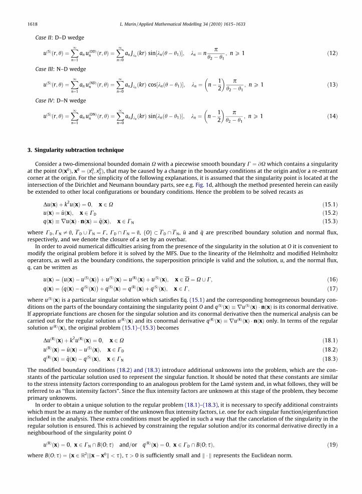
3. Singularity subtraction technique
Consider a two-dimensional bounded domain X with a piecewise smooth boundary C ¼ @X which contains a singularityat the point Oðx0Þ, x0 ¼ ðx0
1; x02Þ, that may be caused by a change in the boundary conditions at the origin and/or a re-entrant
corner at the origin. For the simplicity of the following explanations, it is assumed that the singularity point is located at theintersection of the Dirichlet and Neumann boundary parts, see e.g. Fig. 1d, although the method presented herein can easilybe extended to other local configurations or boundary conditions. Hence the problem to be solved recasts as
DuðxÞ þ k2uðxÞ ¼ 0; x 2 X ð15:1ÞuðxÞ ¼ ~uðxÞ; x 2 CD ð15:2ÞqðxÞ � ruðxÞ � nðxÞ ¼ ~qðxÞ; x 2 CN ð15:3Þ
where CD;CN – ;, CD [ CN ¼ C, CD \ CN ¼ ;, fOg � CD \ CN, ~u and ~q are prescribed boundary solution and normal flux,respectively, and we denote the closure of a set by an overbar.
In order to avoid numerical difficulties arising from the presence of the singularity in the solution at O it is convenient tomodify the original problem before it is solved by the MFS. Due to the linearity of the Helmholtz and modified Helmholtzoperators, as well as the boundary conditions, the superposition principle is valid and the solution, u, and the normal flux,q, can be written as
uðxÞ ¼ uðxÞ � uðSÞðxÞ� �
þ uðSÞðxÞ ¼ uðRÞðxÞ þ uðSÞðxÞ; x 2 X ¼ X [ C; ð16ÞqðxÞ ¼ qðxÞ � qðSÞðxÞ
� �þ qðSÞðxÞ ¼ qðRÞðxÞ þ qðSÞðxÞ; x 2 C; ð17Þ
where uðSÞðxÞ is a particular singular solution which satisfies Eq. (15.1) and the corresponding homogeneous boundary con-ditions on the parts of the boundary containing the singularity point O and qðSÞðxÞ � ruðSÞðxÞ � nðxÞ is its conormal derivative.If appropriate functions are chosen for the singular solution and its conormal derivative then the numerical analysis can becarried out for the regular solution uðRÞðxÞ and its conormal derivative qðRÞðxÞ � ruðRÞðxÞ � nðxÞ only. In terms of the regularsolution uðRÞðxÞ, the original problem (15.1)–(15.3) becomes
DuðRÞðxÞ þ k2uðRÞðxÞ ¼ 0; x 2 X ð18:1ÞuðRÞðxÞ ¼ ~uðxÞ � uðSÞðxÞ; x 2 CD ð18:2ÞqðRÞðxÞ ¼ ~qðxÞ � qðSÞðxÞ; x 2 CN ð18:3Þ
The modified boundary conditions (18.2) and (18.3) introduce additional unknowns into the problem, which are the con-stants of the particular solution used to represent the singular function. It should be noted that these constants are similarto the stress intensity factors corresponding to an analogous problem for the Lamé system and, in what follows, they will bereferred to as ‘‘flux intensity factors”. Since the flux intensity factors are unknown at this stage of the problem, they becomeprimary unknowns.
In order to obtain a unique solution to the regular problem (18.1)–(18.3), it is necessary to specify additional constraintswhich must be as many as the number of the unknown flux intensity factors, i.e. one for each singular function/eigenfunctionincluded in the analysis. These extra conditions must be applied in such a way that the cancelation of the singularity in theregular solution is ensured. This is achieved by constraining the regular solution and/or its conormal derivative directly in aneighbourhood of the singularity point O
uðRÞðxÞ ¼ 0; x 2 CN \ BðO; sÞ and=or qðRÞðxÞ ¼ 0; x 2 CD \ BðO; sÞ; ð19Þ
where BðO; sÞ ¼ fx 2 R2jkx� x0k < sg, s > 0 is sufficiently small and k � k represents the Euclidean norm.

-1.0 -0.5 0.0 0.5 1.0x1
0.0
0.2
0.4
0.6
0.8
1.0
x2
-1.0 -0.5 0.0 0.5 1.0
0.0
0.2
0.4
0.6
0.8
1.0
O
A
BC
D
q = q(an)
u = u(an)
q = q(an)u = u(an)
u = u(an)
-1.0 -0.5 0.0 0.5 1.0x1
-1.0
-0.5
0.0
0.5
1.0
x2
-1.0 -0.5 0.0 0.5 1.0
-1.0
-0.5
0.0
0.5
1.0
O A
BC
D E
u = u(an)
u = u(an)
u = u(an)
u = u(an)
q = q(an)
q = q(an)
-1.0 -0.5 0.0 0.5 1.0x1
-1.0
-0.5
0.0
0.5
1.0
x2
-1.0 -0.5 0.0 0.5 1.0
-1.0
-0.5
0.0
0.5
1.0
O A
BC
D E
q = q(an)
q = q(an)
q = q(an)
q = q(an)
u = u(an)
u = u(an)
-1.0 -0.5 0.0 0.5 1.0x1
0.0
0.2
0.4
0.6
0.8
1.0
x2
-1.0 -0.5 0.0 0.5 1.0
0.0
0.2
0.4
0.6
0.8
1.0
O
A
BC
D
q = q(an)
q = q(an)
q = q(an)
u = u(an)
u = u(an)
Fig. 1. Schematic diagram of the geometry and boundary conditions for the singular problems investigated, namely (a) Example 1: N–D singular problem ina domain containing an edge crack OD with h1 ¼ 0 and h2 ¼ p; (b) Example 2: D–D singular problem in an L-shaped domain with h1 ¼ 0 and h2 ¼ 3p=2; (c)Example 3: N–N singular problem in an L-shaped domain with h1 ¼ 0 and h2 ¼ 3p=2; and (d) Example 4: D–N singular inverse problem in a domaincontaining a V-notch with h1 ¼ 0 and h2 ¼ 11p=12.
L. Marin / Applied Mathematical Modelling 34 (2010) 1615–1633 1619
4. The method of fundamental solutions
The fundamental solutions FH and FMH of the Helmholtz ðk ¼ aþ ib;a 2 R; b ¼ 0Þ and modified Helmholtzðk ¼ aþ ib;a ¼ 0; b 2 RÞ equations, respectively, in the two-dimensional case are given by, see e.g. Fairweather and Kara-georghis [26],
FHðx; yÞ ¼i4
Hð1Þ0 kkx� ykð Þ; x 2 X; y 2 R2 nX; ð20Þ
and
FMHðx; yÞ ¼1
2pK0 kkx� ykð Þ; x 2 X; y 2 R2 nX; ð21Þ
respectively. Here x ¼ ðx1; x2Þ is either a boundary or a domain point, y ¼ ðy1; y2Þ is a source point, Hð1Þ0 is the Hankel functionof the first kind of order zero and K0 is the modified Bessel function of the second kind of order zero.
According to the MFS approach, the regular solution, uðRÞ, in the solution domain is approximated by a linear combinationof fundamental solutions with respect to M source points ym in the form
uðRÞðxÞ �XM
m¼1
cm Fðx; ymÞ; x 2 X; ð22Þ
where F ¼FH in the case of the Helmholtz equation, F ¼FMH in the case of the modified Helmholtz equation, cm 2 R,m ¼ 1; . . . ;M, are the unknown coefficients. Then the regular normal flux on the boundary C can be approximated by

1620 L. Marin / Applied Mathematical Modelling 34 (2010) 1615–1633
qðRÞðxÞ �XM
m¼1
cm Gðx; ymÞ; x 2 C; ð23Þ
where Gðx; yÞ � rxFðx; yÞ � nðxÞ, while G ¼ GH in the case of the Helmholtz equation and G ¼ GMH in the case of the modifiedHelmholtz equation are given by
GHðx; yÞ ¼ �x� yð Þ � nðxÞ½ �ki
4kx� yk Hð1Þ1 kkx� ykð Þ; x 2 C; y 2 R2 nX; ð24Þ
and
GMHðx; yÞ ¼ �x� yð Þ � nðxÞ½ �k2pkx� yk K1 kkx� ykð Þ; x 2 C; y 2 R2 nX; ð25Þ
respectively. Here Hð1Þ1 is the Hankel function of the first kind of order one and K1 is the modified Bessel function of the sec-ond kind of order one.
If the solution domain is a disk of radius r, it was shown in [44,45] that, when the collocation and source points are placeduniformly on the boundary of the disk and on a circle of radius R, R > r, respectively, then the error in the MFS approximationfor L collocation points and L singularities satisfies supx2X ¼ Oððr=RÞLÞ, i.e. exponential convergence is achieved. Furthermore,this result was generalised to two-dimensional regions whose boundaries are analytic Jordan curves by Katsurada [46,47]. Itis worth mentioning that the functional approximation given by Eq. (22) is also consistent, in the sense that this functionalalso approximates accurately the exact solution of the problem not only on the boundary C, but also in the interior of thesolution domain X, see Kondepalli et al. [48] and MacDonell [49]. Moreover, the MFS approximation (22) is capable of repro-ducing various types of solutions to Helmholtz-type equations, such as constant, linear, quadratic, exponential, trigonomet-ric functions, etc., see e.g. Fairweather and Karageorghis [26] and Golberg and Chen [27].
Assume that the singular point O is located between the collocation points xn0D 2 CD and xn0
N 2 CN, and nS singular func-tions/eigenfunctions uðDNÞ
n ðr; hÞ, as well as flux intensities, an, are taken into account, such that the additional constraints forthe regular solution and/or its conormal derivative given by Eq. (19) read as
uðRÞðxn0Nþ1�mÞ ¼ 0 for 2m� 1 2 1; . . . ;nSf g; ð26Þ
and
qðRÞðxn0D�1þmÞ ¼ 0 for 2m 2 1; . . . ;nSf g: ð27Þ
If nD collocation points x‘, ‘ ¼ 1; . . . ;nD, and nN collocation points xnDþ‘, ‘ ¼ 1; . . . ;nN, are chosen on the boundaries CD andCN, respectively, such that L ¼ nD þ nN, and the location of the source points ym, m ¼ 1; . . . ;M, is set then the boundary valueproblem (18.1)–(18.3), together with the additional conditions (19), recasts as a system of ðLþ nSÞ linear algebraic equationswith ðM þ nSÞ unknowns which can be generically written as
A~c ¼ F; ð28Þ
where ~c ¼ ðc1; . . . ; cM ;a1; . . . ;anS Þ 2 RMþnS and the components of the MFS matrix
A 2 RðLþnSÞ�ðMþnSÞ and right-hand side vector F 2 RLþnS are given by
Aij ¼
Fðx‘; ymÞ; ‘ ¼ 1; . . . ; nD; m ¼ 1; . . . ;M
uðDNÞm�Mðr‘; h
‘Þ; ‘ ¼ 1; . . . ; nD; m ¼ M þ 1; . . . ;Mþ nS
Gðx‘; ymÞ; ‘ ¼ nD þ 1; . . . ;nD þ nN; m ¼ 1; . . . ;M
qðDNÞm�Mðr‘; h
‘Þ; ‘ ¼ nD þ 1; . . . ;nD þ nN; m ¼ M þ 1; . . . ;M þ nS
Fðxn0Nþ1�m�N; ymÞ; ‘� L ¼ 2m� 1 2 1; . . . ; nSf g; m ¼ 1; . . . ;M
Gðxn0D�1þm�N ; ymÞ; ‘� L ¼ 2m 2 1; . . . ;nSf g; m ¼ 1; . . . ;M
0; ‘� L 2 1; . . . ;nSf g; m ¼ M þ 1; . . . ;M þ nS
8>>>>>>>>>>>><>>>>>>>>>>>>:
ð29Þ
F‘ ¼~uðx‘Þ; ‘ ¼ 1; . . . ;nD
~qðx‘Þ; ‘ ¼ nD þ 1; . . . ;nD þ nN
0; ‘ ¼ nD þ nN þ 1; . . . ; nD þ nN þ nS
8><>: ð30Þ
Here ðr‘; h‘Þ are the local polar coordinates of the collocation point x‘, ‘ ¼ 1; . . . ; L.It should be noted that in order to uniquely determine the solution ~c of the system of linear algebraic equations (28), i.e.
the coefficients cm, m ¼ 1; . . . ;M, in approximations (22) and (23), and the flux intensity factors an, n ¼ 1; . . . ;nS, in theasymptotic expansions (11)–(14), the total number of collocation points corresponding to the Dirichlet and Neumannboundary conditions, L, and the number of source points, M, must satisfy the inequality M 6 L. It is important to mentionthat the complex MFS + SST system (28) resulting in the case of the Helmholtz equation has been solved by equating bothits real and imaginary parts.

L. Marin / Applied Mathematical Modelling 34 (2010) 1615–1633 1621
In order to implement the MFS, the location of the source points has to be determined and this is usually achieved byconsidering either the static or the dynamic approach. In the static approach, the source points are pre-assigned and keptfixed throughout the solution process, this approach reducing to solving a linear problem [26]. In the dynamic approach,the source points and the unknown coefficients are determined simultaneously during the solution process via a systemof nonlinear equations which may be solved using minimization methods [26]. Therefore, we have decided to employ thestatic approach in our computations with the source points located on a so-called pseudo-boundary which has the sameshape as the boundary of the domain [50].
5. Numerical results and discussion
It is the purpose of this section to present the performance of the modified MFS described in Section 4. To do so, we solvenumerically the direct boundary value problem (15.1)–(15.3) associated with the two-dimensional Helmholtz-type equa-tions in the presence of boundary singularities using the SST + MFS approach.
5.1. Examples
In the case of the singular boundary value problems for both the Helmholtz and the modified Helmholtz equations ana-lysed herein, the solution domains under consideration, X, accessible boundaries, CD and CN, and corresponding analyticalsolutions for uðanÞðxÞ are given as follows:
Example 1. N–D singular problem for the modified Helmholtz equation (a ¼ 0 and b ¼ 1) in a rectangle containing an edgecrack OA, see Fig. 1a:
X ¼ ABCD ¼ ð�1;1Þ � ð0;1Þ ð31:1ÞCD ¼ AB [ CD [ DO ¼ �1;1f g � ð0;1Þ [ ð�1;0Þ � 0f g ð31:2ÞCN ¼ OA [ BC ¼ ð0;1Þ � 0f g [ ð�1;1Þ � 1f g ð31:3ÞuðanÞðxÞ ¼ uðNDÞ
1 ðxÞ � 1:30uðNDÞ2 ðxÞ þ 1:50uðNDÞ
3 ðxÞ � 1:70uðNDÞ4 ðxÞ; x 2 X ð31:4Þ
Example 2. D–D singular problem for the modified Helmholtz equation (a ¼ 0 and b ¼ 1) in an L-shaped domain, see Fig. 1b:
X ¼ OABCDE ¼ ð�1;1Þ � ð0;1Þ [ ð�1;0Þ � ð�1;0� ð32:1ÞCD ¼ OA [ BC [ DE [ EO ¼ ð0;1Þ � 0f g [ ð�1;1Þ � 1f g [ ð�1;0Þ � 0f g [ 0f g � ð�1;0Þ ð32:2ÞCN ¼ AB [ CD ¼ 1f g � ð0;1Þ [ �1f g � ð�1;1Þ ð32:3ÞuðanÞðxÞ ¼ uðDDÞ
1 ðxÞ � 1:30uðDDÞ2 ðxÞ � 1:70uðDDÞ
4 ðxÞ; x 2 X ð32:4Þ
Example 3. N–N singular problem for the Helmholtz equation (a ¼ 1 and b ¼ 0) in an L-shaped domain, see Fig. 1c:
X ¼ OABCDE ¼ ð�1;1Þ � ð0;1Þ [ ð�1;0Þ � ð�1;0� ð33:1ÞCD ¼ AB [ CD ¼ 1f g � ð0;1Þ [ �1f g � ð�1;1Þ ð33:2ÞCN ¼ OA [ BC [ DE [ EO ¼ ð0;1Þ � 0f g [ ð�1;1Þ � 1f g [ ð�1;0Þ � 0f g [ 0f g � ð�1;0Þ ð33:3ÞuðanÞðxÞ ¼ uðNNÞ
1 ðxÞ þ 1:50uðNNÞ2 ðxÞ � 0:50uðNNÞ
4 ðxÞ; x 2 X ð33:4Þ
Example 4. D–N singular problem for the Helmholtz equation (a ¼ 1 and b ¼ 0) in a rectangle containing a V-notch with there-entrant angle 2x ¼ p=6, see Fig. 1d:
X ¼ OABCD ¼ ð�1;1Þ � ð0;1Þ n DODD0 ð34:1ÞCN ¼ AB [ CD [ DO ¼ 1f g � ð0;1Þ [ �1f g � ðsin x;1Þ [ ð�q;q sinxÞ 0 < q < 1jf g ð34:2ÞCD ¼ OA [ BC ¼ ð0;1Þ � 0f g [ ð�1;1Þ � �1f g ð34:3ÞuðanÞðxÞ ¼ uðDNÞ
2 ðxÞ � 1:50uðDNÞ3 ðxÞ þ 1:30uðDNÞ
4 ðxÞ; x 2 X ð34:4Þ
It is important to mention that Examples 1–4 have been chosen such that �k2 is not an eigenvalue of the N–D, D–D, N–Nand D–N problems, respectively, for the Laplacian in the corresponding domains. All examples analysed in this study containa singularity at the origin Oð0;0Þwhich is caused by the nature of the analytical solutions considered, i.e. the analytical solu-tions are given as linear combinations of the first four singular functions/eigenfunctions satisfying homogeneous boundaryconditions on the edges of the wedge, as well as by a sharp corner in the boundary (Examples 2–4) or by an abrupt change inthe boundary conditions at O (Examples 1 and 4), see Fig. 1(a–d).
The singular boundary value problems investigated in this paper have been solved using a uniform distribution of boththe boundary collocation points x‘, ‘ ¼ 1; . . . ; L, and the source points ym, m ¼ 1; . . . ;M, with the mention that the latter were
1622 L. Marin / Applied Mathematical Modelling 34 (2010) 1615–1633
located on a so-called pseudo-boundary, CS, which has the same shape as the boundary C of the solution domain and is sit-uated at the distance d > 0 from C, see e.g. Tankelevich et al. [50]. In the present computations, the values for the distance dwere set to d ¼ 2 for Examples 1–3, and d ¼ 3 for Example 4. Furthermore, the number of boundary collocation points wasset to:
(i) L ¼ 120 for Examples 1 and 4, such that L=3 ¼ 40 and L=6 ¼ 20 collocation points are situated on each of the bound-aries BC and OA, AB, CD, DA and OD, respectively;
(ii) L ¼ 154 for Examples 2 and 3, such that 19 and 39 collocation points are situated on each of the boundaries OA, AB, DEand EO, and BC and CD, respectively.
In addition, for all examples investigated throughout this study, the number of source points, M, was taken to be equal tothat of the boundary collocation points, L, i.e. M ¼ L.
5.2. Accuracy errors
In what follows, we denote by uðnumÞ and qðnumÞ the numerical values for the solution and normal flux, respectively, ob-tained using the least-squares method (LSM), i.e. a direct inversion method, and by subtracting the first nS P 0 singular func-tions/eigenfunctions, with the convention that when nS ¼ 0 then the numerical solution and normal flux are obtained usingthe standard MFS, i.e. without removing the singularity. It should be mentioned that formally the LSM solution, ~cLSM , of theMFS system of linear algebraic Eqs. (28) is given as the solution of the following normal equation
ATA� �
~c ¼ AT F; ð35Þ
in the sense that
~cLSM ¼ ATA� ��1
AT F: ð36Þ
In order to measure the accuracy of the numerical approximation for the solution, uðnumÞ, and normal flux, qðnumÞ, with re-spect to their corresponding analytical values, uðanÞ, and, qðanÞ, respectively, we define the normalized errors
err uðxÞð Þ ¼ juðnumÞðxÞ � uðanÞðxÞjmax
y2eC juðanÞðyÞj ; err qðxÞð Þ ¼ jqðnumÞðxÞ � qðanÞðxÞjmax
y2eC jqðanÞðyÞj ; ð37Þ
for the solution and normal flux, respectively, where eC denotes the set of boundary collocation points, since on using theseerrors divisions by zero and very high errors at points where the solution and/or normal flux have relatively small values areavoided.
Furthermore, we also introduce an error that measures the inaccuracies in the numerical results obtained for the fluxintensity factors, namely the absolute error defined by
ErrðajÞ ¼ jaðnumÞj � ajj: ð38Þ
Here aðnumÞj represents the numerical value for the exact flux intensity factor aj, provided that the latter is available.
5.3. MFS + SST solution for singular problems
The first example investigated contains a singularity at the boundary point O caused by both the abrupt change in theboundary conditions and the nature of the analytical solution, see equation (31.4), in the case of the modified Helmholtzequation. It should be noted that this singularity is of a form which is similar to the case of a sharp re-entrant corner of anglezero, i.e. h2 � h1 ¼ 2p. This may be seen by extending the domain X ¼ ð�1;1Þ � ð0;1Þ using symmetry with respect to the x1-axis, see also Fig. 1a. In this way, a problem is obtained for a square domain containing a crack, namelyeX ¼ ð�1;1Þ � ð�1;1Þ n ½0;1� � f0g with zero flux boundary conditions along the crack ½0;1� � f0g. This problem may alsobe treated by considering the domain eX described above, with the mention that the singular eigenvectors (11) correspondingto Neumann–Neumann boundary conditions along the crack must be used. However, the original domain X and the mixedboundary conditions described in Eqs. (31.2) and (31.3) have been considered in our analysis, i.e. h2 � h1 ¼ p as illustrated inFig. 1a.
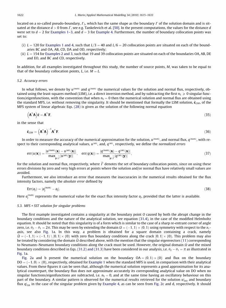
Fig. 2a and b present the numerical solution on the boundary OA ¼ ð0;1Þ � f0g and flux on the boundaryDO ¼ ð�1;0Þ � f0g, respectively, obtained for Example 1 when the standard MFS is used, in comparison with their analyticalvalues. From these figures it can be seen that, although the numerical solution represents a good approximation for its ana-lytical counterpart, the boundary flux does not approximate accurately its corresponding analytical value on DO when nosingular functions/eigenfunctions are subtracted, i.e. nS ¼ 0, and at the same time having an oscillatory behaviour on thispart of the boundary. A similar pattern is observed for the numerical results retrieved for the solution ujDO and boundaryflux qjOA in the case of the singular problem given by Example 4, as can be seen from Fig. 2c and d, respectively. It should
0.0 0.2 0.4 0.6 0.8 1.0x1
0.0
0.2
0.4
0.6
0.8u
Analyticaln S = 0
-1.0 -0.8 -0.6 -0.4 -0.2 0.0x1
-4
-3
-2
-1
0
1
2
q
AnalyticalnS = 0
-1.0 -0.8 -0.6 -0.4 -0.2 0.0x1
-0.3
-0.2
-0.1
0.0
0.1
0.2
0.3
u
AnalyticalnS = 0
0.0 0.2 0.4 0.6 0.8 1.0x1
-0.5
-0.4
-0.3
-0.2
-0.1
0.0
q
Analyticaln S = 0
Fig. 2. Analytical and numerical solutions (a) ujOA, and (b) qjDO, obtained without subtracting any singular functions/eigenfunctions (nS ¼ 0) for the N–Dsingular problem given by Example 1. Analytical and numerical solutions (c) ujDO, and (d) qjOA, obtained without subtracting any singular functions/eigenfunctions ðnS ¼ 0Þ for the D–N singular problem given by Example 4.
L. Marin / Applied Mathematical Modelling 34 (2010) 1615–1633 1623
be mentioned that in this case both the numerical solution and the numerical boundary flux are very inaccurate approxima-tions for their analytical values. Although not presented, it is reported that similar results have been obtained for the singularproblems given by Examples 2 and 3, as well as the other unknown boundary solutions and fluxes for all examplesinvestigated.
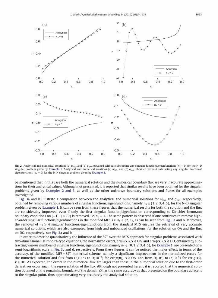
Fig. 3a and b illustrate a comparison between the analytical and numerical solutions for ujOA and qjDO, respectively,obtained by removing various numbers of singular functions/eigenfunctions, namely nS 2 f1;2;3;4;5g, for the N–D singularproblem given by Example 1. It can be seen from these figures that the numerical results for both the solution and the fluxare considerably improved, even if only the first singular function/eigenfunction corresponding to Dirichlet–Neumannboundary conditions on ð�1;1Þ � f0g is removed, i.e. nS ¼ 1. The same pattern is observed if one continues to remove high-er-order singular functions/eigenfunctions in the modified MFS, i.e. nS 2 f2;3g, as can be seen from Fig. 3a and b. Moreover,the removal of nS P 4 singular functions/eigenfunctions from the standard MFS ensures the retrieval of very accuratenumerical solutions, which are also exempted from high and unbounded oscillations, for the solution on OA and the fluxon DO, respectively, see Fig. 3a and b.
In order to describe quantitatively the influence of the SST over the MFS approach for singular problems associated withtwo-dimensional Helmholtz-type equations, the normalized errors, errðuðxÞÞ, x 2 OA, and errðqðxÞÞ, x 2 DO, obtained by sub-tracting various numbers of singular functions/eigenfunctions, namely nS 2 f0;1;2;3;4;5g, for Example 1, are presented on asemi-logarithmic scale in Fig. 3c and d, respectively. From these figures it can be noticed the major effect, in terms of theaccuracy, of the modified MFS + SST numerical scheme, namely a significant improvement in the normalized errors forthe numerical solution and flux from Oð10�2Þ to Oð10�8Þ for errðuðxÞÞ, x 2 OA, and from Oð100Þ to Oð10�6Þ for errðqðxÞÞ,x 2 DO. As expected, the errors in the numerical flux are larger than those in the numerical solution due to the first-orderderivatives occurring in the representation of the flux. Although not presented herein, it is reported that the numerical solu-tion obtained on the remaining boundary of the domain X has the same accuracy as that presented on the boundary adjacentto the singular point, thus approximating very accurately the analytical solution.

0.0 0.2 0.4 0.6 0.8 1.0x1
0.0
0.2
0.4
0.6
0.8u
AnalyticalnS = 1nS = 2nS = 3nS = 4nS = 5
-1.0 -0.8 -0.6 -0.4 -0.2 0.0x1
-1
0
1
2
3
q
Analytical n S = 1nS = 2 n S = 3nS = 4 n S = 5
0.0 0.2 0.4 0.6 0.8 1.0x1
10-8
10-6
10-4
10-2
Nor
mal
ized
erro
r err(
u(x)
)
n S = 0 n S = 1n S = 2 n S = 3n S = 4 n S = 5
-1.0 -0.8 -0.6 -0.4 -0.2 0.0x1
10-8
10-6
10-4
10-2
100
Nor
mal
ized
erro
r err(
q(x)
)nS = 0 n S = 1nS = 2 n S = 3nS = 4 n S = 5
Fig. 3. Analytical and numerical solutions (a) ujOA, and (b) qjDO, and the corresponding normalized errors (c) errðuðxÞÞ, x 2 OA, and (d) errðqðxÞÞ, x 2 DO,obtained by subtracting various numbers of singular functions/eigenfunctions, namely nS 2 f1;2;3;4;5g, for the N–D singular problem given by Example 1.
1624 L. Marin / Applied Mathematical Modelling 34 (2010) 1615–1633
Fig. 4(a–f) show the contour lines for the normalized error errðuðxÞÞ at internal points x 2 Xint � X located in a neighbour-hood of the singularity point O, namely Xint ¼ ð�10�2;10�2Þ � ð0;10�2Þ, as a function of the number of singular functions/eigenfunctions nS subtracted from the standard MFS. These figures clearly emphasize the remarkable numerical results ob-tained also for the solution at internal points situated in the vicinity of the origin, by employing the combined MFS + SSTtechnique. It can be seen form these figures that a significant improvement in the accuracy of the numerical solution takesplace, namely from Oð100Þ for nS ¼ 0 to Oð10�6Þ and Oð10�8Þ for nS ¼ 4 and nS ¼ 5, respectively. In the case of Example 1, veryaccurate numerical results are also obtained for the exact flux intensity factors given by Eq. (31.4), as can be seen from Table1, which presents the numerical values, aðnumÞ
j , for the flux intensity factors, aj, as well as the corresponding absolute errorsdefined by Eq. (38).
Both the second and the third examples investigated in this paper contain a singularity at the origin O which is caused bya sharp corner in the boundary, as well as the nature of the analytical solutions corresponding to these problems, i.e. theanalytical solutions are given as linear combinations of the first four singular functions satisfying homogeneous Dirichletor Neumann boundary conditions on the edges of the wedge for Examples 2 and 3, respectively. The analytical and numericalfluxes on the boundaries EO ¼ f0g � ð�1;0Þ and OA ¼ ð0;1Þ � f0g obtained for Example 2 by subtracting nS 2 f1;2;3;4;5gsingular functions/eigenfunctions are illustrated in Fig. 5a and b, respectively. Although not presented, it is worth mention-ing that the numerical flux obtained on EO [ OA using the standard MFS, i.e. nS ¼ 0, exhibits very high oscillations in theneighbourhood of the singular point and hence it represents an inaccurate approximation for the analytical flux. Even whenthe first singular function/eigenfunction is subtracted from the MFS, i.e. nS ¼ 1, the numerically retrieved solutions for qjEO
and qjOA are still oscillatory and inaccurate. Moreover, from Fig. 5a and b it can be seen that also for nS ¼ 1 oscillations in thenumerical flux occur even far from the singularity, namely in the vicinity of the points x ¼ ð0;�1Þ and x ¼ ð1;0Þ. However,this difficulty can be overcome if instead of the standard MFS, the modified MFS described in the previous section is em-ployed with nS P 2. From Fig. 5a and b it can be noticed that the accuracy in the numerical flux is slightly improved fornS 2 f2;3g and a very good accuracy in the numerical flux on the boundary adjacent to the origin is attained as nS approaches

1.86E+001.88E+00
1.89E+001.90E+00
1.90E+001.91E+00
1.90E+00
1.91E+00
1.91
E+00
1.92E+00
1.91E+00
1.92E+00
-1.0*10-2 -5.0*10-3 0.0*100 5.0*10-3 1.0*10-2
x1
2.0*10-3
4.0*10-3
6.0*10-3
8.0*10-3
1.0*10-2
x 2 2.60E-012.60E-012.59E-01
2.56E-012.54E-01
2.50E-012.49E-01
2.48
E-01
2.48E-012.48E-01
2.49
E-01
2.48E-01
-1.0*10-2 -5.0*10-3 0.0*100 5.0*10-3 1.0*10-2
x1
2.0*10-3
4.0*10-3
6.0*10-3
8.0*10-3
1.0*10-2
x 2
2.79E-012.79E-01
2.80E-012.81E-01
2.81E-012.81E-01
2.82
E-01
2.81E-012.81E-01
2.80E-01
2.79
E-01
2.79E-012.79E-01
2.78E-01
2.80E-01
2.81E-01
-1.0*10-2 -5.0*10-3 0.0*100 5.0*10-3 1.0*10-2
x1
2.0*10-3
4.0*10-3
6.0*10-3
8.0*10-3
1.0*10-2
x 2 1.44E-021.47E-021.50E-021.53E-02
1.56E-02
1.56
E-02
1.59E-02
1.58
E-02
1.60E
-02
1.59E-02
1.59E-02
-1.0*10-2 -5.0*10-3 0.0*100 5.0*10-3 1.0*10-2
x1
2.0*10-3
4.0*10-3
6.0*10-3
8.0*10-3
1.0*10-2
x 2
2.52E-062.48E-06
2.43E-06
2.37E-06
2.32E-06
2.26E-06
2.23
E-06
2.21E-06
2.22
E-06
60-E12.2
2.20E-06
2.23
E-06
-1.0*10-2 -5.0*10-3 0.0*100 5.0*10-3 1.0*10-2
x1
2.0*10-3
4.0*10-3
6.0*10-3
8.0*10-3
1.0*10-2
x 2
1.26E-071.18E-07
1.05E-078.56E-08
7.66E-08
7.05
E-08
5.83
E-08
7.66E-089.46E-08
1.05E-07
1.18
E-07
1.26E-07
1.39E-07
1.12E-079.46E-08
7.66E-08
-1.0*10-2 -5.0*10-3 0.0*100 5.0*10-3 1.0*10-2
x1
2.0*10-3
4.0*10-3
6.0*10-3
8.0*10-3
1.0*10-2
x 2
Fig. 4. Contour plot of the normalized error, errðuðxÞÞ, in the neighbourhood, Xint � X, of the singular point O, obtained by subtracting various numbers ofsingular functions/eigenfunctions, namely (a) nS ¼ 0, (b) nS ¼ 1, (c) nS ¼ 2, (d) nS ¼ 3, (e) nS ¼ 4 and (f) nS ¼ 5, for the N–D singular problem given byExample 1.
Table 1The numerically retrieved values, aðnumÞ
j , 1 6 j 6 4, for the flux intensity factors and the corresponding absolute errors, ErrðajÞ, 1 6 j 6 4, obtained using themodified MFS and subtracting various numbers of singular functions/eigenfunctions, namely nS 2 f1;2;3;4; 5g, for the N–D singular problem given by Example1.
nS aðnumÞ1
Errða1Þ aðnumÞ2
Errða2Þ aðnumÞ3
Errða3Þ aðnumÞ4
Errða4Þ
1 1.1538 0:15� 100 – – – – – –
2 1.1681 0:16� 100 �1:6624 0:66� 100 – – – –
3 1.0163 0:01� 100 �1:5749 0:27� 100 1:1819 0:31� 100 – –
4 1.0000 0:10� 10�7 �1:3001 0:54� 10�4 1.5000 0:30� 10�4 �1:6998 0:15� 10�3
5 1.0000 0:34� 10�5 �1:3000 0:15� 10�4 1.4999 0:96� 10�4 �1:6994 0:56� 10�3
L. Marin / Applied Mathematical Modelling 34 (2010) 1615–1633 1625

-1.0 -0.8 -0.6 -0.4 -0.2 0.0x2
-0.6
-0.4
-0.2
0.0
0.2
q
Analytical nS = 1nS = 2 nS = 3nS = 4 nS = 5
0.0 0.2 0.4 0.6 0.8 1.0x1
-0.8
-0.6
-0.4
-0.2
q
Analytical nS = 1nS = 2 nS = 3nS = 4 nS = 5
-1.0 -0.8 -0.6 -0.4 -0.2 0.0x2
10-8
10-6
10-4
10-2
100
Nor
mal
ized
erro
r err(
q(x)
)
n S = 0 n S = 1n S = 2 n S = 3n S = 4 n S = 5
0.0 0.2 0.4 0.6 0.8 1.0x1
10-8
10-6
10-4
10-2
100
Nor
mal
ized
erro
r err(
q(x)
)
nS = 0 nS = 1nS = 2 nS = 3nS = 4 nS = 5
Fig. 5. Analytical and numerical solutions (a) qjEO, and (b) qjOA, and the corresponding normalized errors (c) errðqðxÞÞ, x 2 EO, and (d) errðqðxÞÞ, x 2 OA,obtained by subtracting various numbers of singular functions/eigenfunctions, namely nS 2 f1;2;3;4;5g, for the D–D singular problem given by Example 2.
1626 L. Marin / Applied Mathematical Modelling 34 (2010) 1615–1633
four, i.e. the number of singular functions satisfying homogeneous Dirichlet boundary conditions on the edges of the wedgeused in expression (32.4) for the analytical solution.
Similar conclusions can also be drawn from Fig. 5c and d which present the results shown in Fig. 5a and b in terms of thenormalized errors errðqðxÞÞ, x 2 EO, and errðqðxÞÞ, x 2 OA, respectively, as defined by formula (37). Also, from these figures itcan be seen the major effect, in terms of accuracy, of the SST applied to the standard MFS, namely a significant improvementin the accuracy of the flux from Oð100Þ to Oð10�8Þ for errðqðxÞÞ, x 2 EO [ OA. The numerical results obtained for the exact fluxintensity factors given by Eq. (32.4) are very accurate as the number of singular functions/eigenfunctions, nS, increases andapproaches four and this can be clearly noticed from Table 2, which tabulates the numerical values, aðnumÞ
j , for the flux inten-sity factors, aj, as well as the corresponding absolute errors for Example 2.
In Example 3 a singular problem in the same L-shaped domain as that considered in Example 2 is analysed, butwith Neumman–Neumann boundary conditions on the edges EO and OA adjacent to the singularity point O, for the
Table 2The numerically retrieved values, aðnumÞ
j , 1 6 j 6 4, for the flux intensity factors and the corresponding absolute errors, ErrðajÞ, 1 6 j 6 4, obtained using themodified MFS and subtracting various numbers of singular functions/eigenfunctions, namely nS 2 f1;2;3;4;5g, for the D–D singular problem given by Example2.
nS aðnumÞ1
Errða1Þ aðnumÞ2
Errða2Þ aðnumÞ3
Errða3Þ aðnumÞ4
Errða4Þ
1 0.3374 0:97� 100 – – – – – –
2 1.2299 0:23� 100 �1:4525 0:15� 100 – – – –
3 0.8836 0:12� 100 �1:3265 0:26� 10�1 �0:38� 100 0:38� 100 – –
4 1.0000 0:16� 10�5 �1:3000 0:12� 10�6 0:17� 10�5 0:17� 10�5 �1:7000 0:85� 10�6
5 1.0000 0:12� 10�5 �1:3000 0:13� 10�5 �0:56� 10�6 0:56� 10�6 �1:7000 0:17� 10�5

L. Marin / Applied Mathematical Modelling 34 (2010) 1615–1633 1627
two-dimensional Hemholtz equation. Fig. 6a and b show the analytical and numerical solutions on the boundaries EO andOA, respectively, obtained for Example 3 when the modified MFS is used, i.e. nS 2 f1;2;3;4;5g. Although not presented, itshould be mentioned that the numerical solution retrieved without removing the singularities, i.e. nS ¼ 0, is an inaccurateapproximation for its corresponding analytical value not only in the vicinity of the singularity point O, but also on the entireedges adjacent to it. This difficulty can also be alleviated by using the MFS in conjunction with the SST. By comparing Fig. 5aand b and Fig. 6a and b, it can be seen that Example 3 is less severe than Example 2, in the sense that, as expected, the knowl-edge of Dirichlet data on the boundary EO [ OA provides more inaccurate numerical results on this portion of the boundarythan those obtained by given Neumann data on EO [ OA. The same conclusion can be drawn form Fig. 5c and d and Fig. 6cand d which illustrate the numerical results mentioned above in terms of the normalized errors errðuðxÞÞ, x 2 EO, anderrðuðxÞÞ, x 2 OA, respectively, for nS 2 f0;1;2;3;4;5g singular functions/eigenfunctions subtracted.
Fig. 7(a–f) present the contour lines for the normalized error errðuðxÞÞ at internal points situated in a neighbourhood ofthe singularity point O, i.e. x 2 Xint ¼ ð�10�2;10�2Þ � ð0;10�2Þ [ ð�10�2;0Þ � ð�10�2;0�, as a function of the number, nS, ofsingular functions/eigenfunctions subtracted from the standard MFS. These figures clearly illustrate the remarkable numer-ical results obtained also for the solution at internal points situated in the vicinity of the origin, by employing the combinedMFS + SST technique, thus showing a significant improvement in the accuracy of the numerical solution uðxÞ, x 2 Xint . Moreprecisely, the normalized error errðuðxÞÞ, x 2 Xint , decreases from Oð100Þ for nS ¼ 0 to Oð10�7Þ and Oð10�8Þ for nS ¼ 4 andnS ¼ 5, respectively. For Example 3, very accurate numerical results are also obtained for the exact flux intensity factors givenby Eq. (33.4), as can be seen from Table 3, which presents the numerical values, aðnumÞ
j , 1 6 j 6 4 for the flux intensity factors,aj, and their corresponding absolute errors ErrðajÞ, 1 6 j 6 4.
Finally, the last example investigated in this paper is the most severe one, in the sense that the singularity at the origin Ois caused by the abrupt change in the boundary conditions (i.e. Dirichlet and Neumann boundary conditions on OA and DO,respectively), a sharp corner in the boundary, see Fig. 1d, as well as the nature of the analytical solution, see Eq. (34.4), in thecase of the Helmholtz equation. As shown in Fig. 2c and d, both the numerical solution on DO and the numerical boundary
-1.0 -0.8 -0.6 -0.4 -0.2 0.0x2
-0.3
-0.2
-0.1
0.0
0.1
0.2
0.3
u Analytical nS = 1nS = 2 nS = 3nS = 4 nS = 5
0.0 0.2 0.4 0.6 0.8 1.0x1
0.2
0.4
0.6
0.8
1.0
u
AnalyticalnS = 1nS = 2nS = 3nS = 4nS = 5
-1.0 -0.8 -0.6 -0.4 -0.2 0.0x2
10-8
10-6
10-4
10-2
100
Nor
mal
ized
erro
r err(
u(x)
)
nS = 0 nS = 1nS = 2 nS = 3nS = 4 nS = 5
0.0 0.2 0.4 0.6 0.8 1.0x1
10-8
10-6
10-4
10-2
100
Nor
mal
ized
erro
r err(
u(x)
)
nS = 0 nS = 1nS = 2 nS = 3nS = 4 nS = 5
Fig. 6. Analytical and numerical solutions (a) ujEO, and (b) ujOA, and the corresponding normalized errors (c) errðuðxÞÞ, x 2 EO, and (d) errðuðxÞÞ, x 2 OA,obtained by subtracting various numbers of singular functions/eigenfunctions, namely nS 2 f1;2;3;4;5g, for the N–N singular problem given by Example 3.

6.94E+006.95E+00
6.97E+00
6.97E+00
6.95E+00
6.90E+00
6.89E+006.90E+00
6.92E+00
-1.0*10-2 0.0*100 1.0*10-2
x1
-1.0*10-2
-5.0*10-3
0.0*100
5.0*10-3
1.0*10-2
x 2
9.54E+00
9.55E+009.56E+00
9.56E+00
9.56E+00
9.54E+009.56E+00
9.57E+00
-1.0*10-2 0.0*100 1.0*10-2
x1
-1.0*10-2
-5.0*10-3
0.0*100
5.0*10-3
1.0*10-2
x 2
9.68E-019.69E-01
9.69E-019.70E-01
9.69E-01
9.69E-019.70E-019.71E-01
-1.0*10-2 0.0*100 1.0*10-2
x1
-1.0*10-2
-5.0*10-3
0.0*100
5.0*10-3
1.0*10-2
x 2
8.08E-018.08E-01
8.08E-018.08E-01
8.08E-018.08E-018.09E-01
-1.0*10-2 0.0*100 1.0*10-2
x1
-1.0*10-2
-5.0*10-3
0.0*100
5.0*10-3
1.0*10-2
x 2
9.33E-079.33E-07
9.33E-079.33E-07
9.34E-07
9.34E-07
-1.0*10-2 0.0*100 1.0*10-2
x1
-1.0*10-2
-5.0*10-3
0.0*100
5.0*10-3
1.0*10-2
x 2
9.62E-089.69E-08
9.73E-089.72E-08
9.77E-08
9.69E-089.77E-08
-1.0*10-2 0.0*100 1.0*10-2
x1
-1.0*10-2
-5.0*10-3
0.0*100
5.0*10-3
1.0*10-2
x 2
Fig. 7. Contour plot of the normalized error, errðuðxÞÞ, in the neighbourhood, Xint � X, of the singular point O, obtained by subtracting various numbers ofsingular functions/eigenfunctions, namely (a) nS ¼ 0, (b) nS ¼ 1, (c) nS ¼ 2, (d) nS ¼ 3, (e) nS ¼ 4 and (f) nS ¼ 5, for the N–N singular problem given byExample 3.
1628 L. Marin / Applied Mathematical Modelling 34 (2010) 1615–1633
flux on OA obtained without removing any singular function/eigenfunction, i.e. nS ¼ 0, represent highly inaccurate approx-imations for their analytical values. Again, this situation can be overcome by employing the modified MFS presented in Sec-tion 4. Consequently, the numerical solution uðnumÞjDO and numerical boundary flux qðnumÞjOA approach their corresponding
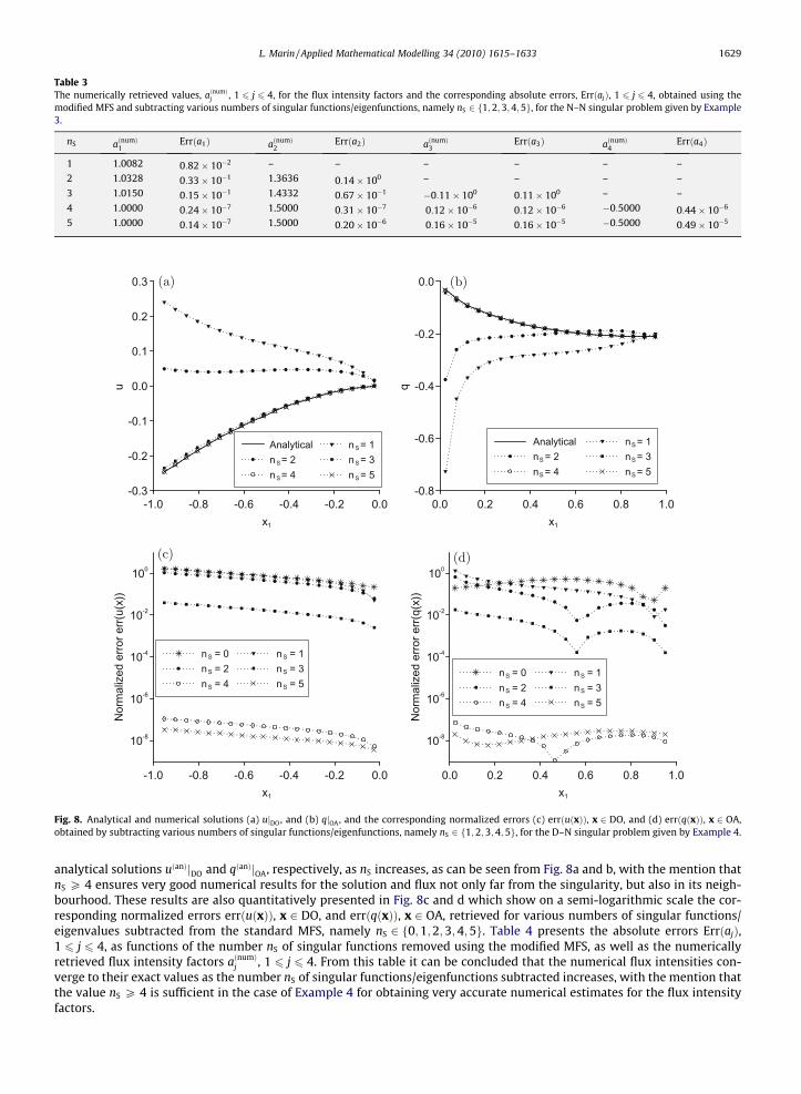
Table 3The numerically retrieved values, aðnumÞ
j , 1 6 j 6 4, for the flux intensity factors and the corresponding absolute errors, ErrðajÞ, 1 6 j 6 4, obtained using themodified MFS and subtracting various numbers of singular functions/eigenfunctions, namely nS 2 f1;2; 3;4;5g, for the N–N singular problem given by Example3.
nS aðnumÞ1
Errða1Þ aðnumÞ2
Errða2Þ aðnumÞ3
Errða3Þ aðnumÞ4
Errða4Þ
1 1.0082 0:82� 10�2 – – – – – –
2 1.0328 0:33� 10�1 1.3636 0:14� 100 – – – –
3 1.0150 0:15� 10�1 1.4332 0:67� 10�1 �0:11� 100 0:11� 100 – –
4 1.0000 0:24� 10�7 1.5000 0:31� 10�7 0:12� 10�6 0:12� 10�6 �0:5000 0:44� 10�6
5 1.0000 0:14� 10�7 1.5000 0:20� 10�6 0:16� 10�5 0:16� 10�5 �0:5000 0:49� 10�5
-1.0 -0.8 -0.6 -0.4 -0.2 0.0x1
-0.3
-0.2
-0.1
0.0
0.1
0.2
0.3
u
Analytical nS = 1n S = 2 nS = 3n S = 4 nS = 5
0.0 0.2 0.4 0.6 0.8 1.0x1
-0.8
-0.6
-0.4
-0.2
0.0
q
Analytical nS = 1nS = 2 nS = 3nS = 4 nS = 5
-1.0 -0.8 -0.6 -0.4 -0.2 0.0x1
10-8
10-6
10-4
10-2
100
Nor
mal
ized
erro
r err(
u(x)
)
nS = 0 nS = 1nS = 2 nS = 3nS = 4 nS = 5
0.0 0.2 0.4 0.6 0.8 1.0x1
10-8
10-6
10-4
10-2
100
Nor
mal
ized
erro
r err(
q(x)
)
nS = 0 nS = 1nS = 2 nS = 3nS = 4 nS = 5
Fig. 8. Analytical and numerical solutions (a) ujDO, and (b) qjOA, and the corresponding normalized errors (c) errðuðxÞÞ, x 2 DO, and (d) errðqðxÞÞ, x 2 OA,obtained by subtracting various numbers of singular functions/eigenfunctions, namely nS 2 f1;2;3;4;5g, for the D–N singular problem given by Example 4.
L. Marin / Applied Mathematical Modelling 34 (2010) 1615–1633 1629
analytical solutions uðanÞjDO and qðanÞjOA, respectively, as nS increases, as can be seen from Fig. 8a and b, with the mention thatnS P 4 ensures very good numerical results for the solution and flux not only far from the singularity, but also in its neigh-bourhood. These results are also quantitatively presented in Fig. 8c and d which show on a semi-logarithmic scale the cor-responding normalized errors errðuðxÞÞ, x 2 DO, and errðqðxÞÞ, x 2 OA, retrieved for various numbers of singular functions/eigenvalues subtracted from the standard MFS, namely nS 2 f0;1;2;3;4;5g. Table 4 presents the absolute errors ErrðajÞ,1 6 j 6 4, as functions of the number nS of singular functions removed using the modified MFS, as well as the numericallyretrieved flux intensity factors aðnumÞ
j , 1 6 j 6 4. From this table it can be concluded that the numerical flux intensities con-verge to their exact values as the number nS of singular functions/eigenfunctions subtracted increases, with the mention thatthe value nS P 4 is sufficient in the case of Example 4 for obtaining very accurate numerical estimates for the flux intensityfactors.
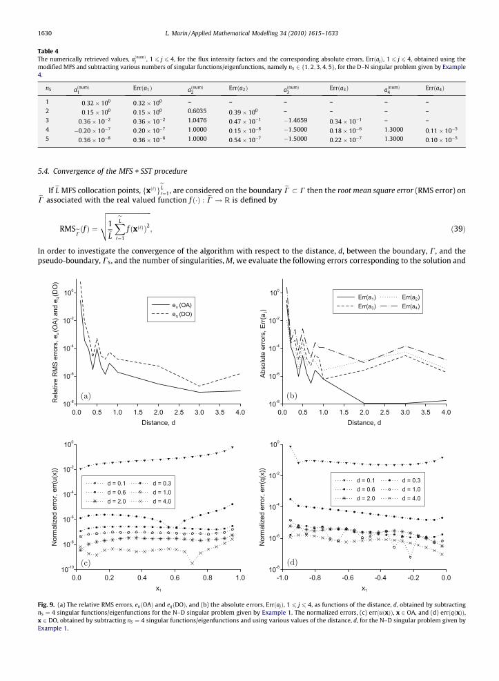
Table 4The numerically retrieved values, aðnumÞ
j , 1 6 j 6 4, for the flux intensity factors and the corresponding absolute errors, ErrðajÞ, 1 6 j 6 4, obtained using themodified MFS and subtracting various numbers of singular functions/eigenfunctions, namely nS 2 f1;2;3; 4;5g, for the D–N singular problem given by Example4.
nS aðnumÞ1
Errða1Þ aðnumÞ2
Errða2Þ aðnumÞ3
Errða3Þ aðnumÞ4
Errða4Þ
1 0:32� 100 0:32� 100 – – – – – –
2 0:15� 100 0:15� 100 0.6035 0:39� 100 – – – –
3 0:36� 10�2 0:36� 10�2 1.0476 0:47� 10�1 �1:4659 0:34� 10�1 – –
4 �0:20� 10�7 0:20� 10�7 1:0000 0:15� 10�8 �1:5000 0:18� 10�6 1:3000 0:11� 10�5
5 0:36� 10�8 0:36� 10�8 1:0000 0:54� 10�7 �1:5000 0:22� 10�7 1:3000 0:10� 10�5
1630 L. Marin / Applied Mathematical Modelling 34 (2010) 1615–1633
5.4. Convergence of the MFS + SST procedure
If eL MFS collocation points, fxð‘ÞgeL‘¼1, are considered on the boundary eC � C then the root mean square error (RMS error) oneC associated with the real valued function f ð�Þ : eC ! R is defined by
Nor
mal
ized
erro
r, er
r(u(x
))
Fig. 9.nS ¼ 4x 2 DOExampl
RMSeCðf Þ ¼ffiffiffiffiffiffiffiffiffiffiffiffiffiffiffiffiffiffiffiffiffiffiffiffiffiffiffi1eLXeL‘¼1
f xð‘Þð Þ2vuut
; ð39Þ
In order to investigate the convergence of the algorithm with respect to the distance, d, between the boundary, C, and thepseudo-boundary, CS, and the number of singularities, M, we evaluate the following errors corresponding to the solution and
0.0 0.5 1.0 1.5 2.0 2.5 3.0 3.5 4.0Distance, d
10-8
10-6
10-4
10-2
100
Rel
ativ
e R
MS
erro
rs, e
u(O
A) a
nd e
q(D
O)
eu (OA)eq (DO)
0.0 0.5 1.0 1.5 2.0 2.5 3.0 3.5 4.0Distance, d
10-8
10-6
10-4
10-2
100
Abso
lute
erro
rs, E
rr(a
j)
Err(a1) Err(a2)Err(a3) Err(a4)
0.0 0.2 0.4 0.6 0.8 1.0x1
10-10
10-8
10-6
10-4
10-2
100
d = 0.1 d = 0.3d = 0.6 d = 1.0d = 2.0 d = 4.0
-1.0 -0.8 -0.6 -0.4 -0.2 0.0x1
10-8
10-6
10-4
10-2
100
Nor
mal
ized
erro
r, er
r(q(x
))
d = 0.1 d = 0.3d = 0.6 d = 1.0d = 2.0 d = 4.0
(a) The relative RMS errors, euðOAÞ and eqðDOÞ, and (b) the absolute errors, ErrðajÞ, 1 6 j 6 4, as functions of the distance, d, obtained by subtractingsingular functions/eigenfunctions for the N–D singular problem given by Example 1. The normalized errors, (c) errðuðxÞÞ, x 2 OA, and (d) errðqðxÞÞ,, obtained by subtracting nS ¼ 4 singular functions/eigenfunctions and using various values of the distance, d, for the N–D singular problem given bye 1.

L. Marin / Applied Mathematical Modelling 34 (2010) 1615–1633 1631
flux on each portion of boundary adjacent to the singular point (generically denoted by eC), which are defined as relative RMSerrors, i.e.
euðeCÞ ¼ RMSeC uðnumÞ � uðanÞ� �RMSeC uðanÞð Þ ; eqðeCÞ ¼ RMSeC qðnumÞ � qðanÞ� �
RMSeC qðanÞð Þ ; ð40Þ
Fig. 9a shows the relative RMS errors euðOAÞ and eqðDOÞ, obtained by subtracting nS ¼ 4 singular functions/eigenfunc-tions, as functions of the distance, d, to the pseudo-boundary where the MFS source points are located, for Example 1. Itcan be seen from this figure that both errors euðOAÞ and eqðDOÞ defined by relation (40) decrease as the distance d increases,with the mention that a very good accuracy of the numerical results is achieved for d P 0:3. Also, as expected eu < eq for alld > 0, i.e. fluxes are more inaccurate than potential solutions. The same convergent behaviour with respect to increasing thedistance between the boundary, C, of the solution domain and the pseudo-boundary, CS, is exhibited by the absolute errors,ErrðajÞ, 1 6 j 6 4, and this is presented in Fig. 9b. The convergence of the MFS + SST algorithm with respect to increasing d hasalso a pointwise character. This feature of the proposed MFS + SST procedure is clearly illustrated in Fig. 9c and d which pres-ent the normalized errors errðuðxÞÞ, x 2 OA, and errðqðxÞÞ, x 2 DO, respectively, obtained using nS ¼ 4 and various values ofthe distance between C and CS, namely d 2 f0:1;0:3;0:6;1:0;2:0;4:0g, for the N–D singular problem given by Example 1.Similar results have been obtained for the other examples considered in this study and, therefore, they have not presentedherein.
Overall, from the examples investigated in this section and the numerical results presented in Figs. 2–9 and Tables 1–4 itcan be concluded that the SST applied to the standard MFS is a very suitable method for solving boundary value problemsexhibiting singularities caused by the presence of sharp corners in the boundary of the solution domain and/or abruptchanges in the boundary conditions, for both the Helmholtz and the modified Helmholtz equations. The numerical solutionsand fluxes retrieved using the MFS + SST technique are very good approximations for their analytical values on the entireboundary, they are exempted from oscillations in the neighbourhood of the singular point and there is no need of furthermesh refinement in the vicinity of the singularities. Although not illustrated numerically here, it should be noted that theproposed modified MFS described in Section 4 has provided very accurate results for some other tested cases for two-dimen-sional Helmholtz-type equations. It should be mentioned, however, that for singular boundary value problems associatedwith Helmholtz-type equations the numerical results obtained using the proposed MFS + SST procedure are more inaccuratethan those retrieved by employing the BEM + SST algorithm introduced by Marin et al. [22].
6. Conclusions
In this study, the MFS was applied for solving accurately and stably problems associated with the two-dimensional Helm-holtz-type equations in the presence of boundary singularities. The existence of such boundary singularities affects adverselythe accuracy and convergence of standard numerical methods. Consequently, the MFS solutions to such problems and/ortheir corresponding derivatives, obtained by a direct inversion of the MFS system (i.e. by the LSM or the equivalent normalequation), may have unbounded values in the vicinity of the singularity. This difficulty was overcome by subtracting fromthe original MFS solution the corresponding singular functions, as given by the asymptotic expansion of the solution nearthe singularity point. Hence, in addition to the original MFS unknowns, new unknowns were introduced, namely the so-called flux intensity factors. Consequently, the original MFS system was extended by considering a number of additionalequations which equals the number of flux intensity factors introduced and specifically imposes the type of singularity ana-lysed in the vicinity of the singularity point. The proposed MFS + SST was implemented and analysed for problems associatedwith both the Helmholtz and the modified Helmholtz equations in two-dimensional domains containing an edge crack or aV-notch, as well as an L-shaped domain.
From the numerical results presented in this study, we can conclude that the advantages of the proposed method overother methods, such as mesh refinement in the neighbourhood of the singularity, the use of singular BEMs and/or FEMsetc., are the high accuracy which can be obtained even when employing a small number of collocation points and sources,and the simplicity of the computational scheme. A possible drawback of the present method is the difficulty in extending themethod to deal with singularities in three-dimensional problems since such an extension is not straightforward.
Acknowledgement
The financial support received from the Romanian Ministry of Education, Research and Innovation through IDEI Pro-gramme, Exploratory Research Projects, Grant PN II–ID–PCE–1248/2008, is gratefully acknowledged.
References
[1] T. Apel, A.-M. Sändig, J.R. Whiteman, Graded mesh refinement and error estimates for finite element solution of elliptic boundary value problems innon-smooth domains, Math. Methods Appl. Sci. 19 (1996) 63–85.
[2] T. Apel, S. Nicaise, The finite element method with anisotropic mesh grading for elliptic problems in domains with corners and edges, Math. MethodsAppl. Sci. 21 (1998) 519–549.
[3] D.E. Beskos, Boundary element method in dynamic analysis: Part II (1986–1996), ASME Appl. Mech. Rev. 50 (1997) 149–197.

1632 L. Marin / Applied Mathematical Modelling 34 (2010) 1615–1633
[4] J.T. Chen, M.T. Liang, I.L. Chen, S.W. Chyuan, K.H. Chen, Dual boundary element analysis of wave scattering from singularities, Wave Motion 30 (1999)367–381.
[5] J.T. Chen, F.C. Wong, Dual formulation of multiple reciprocity method for the acoustic mode of a cavity with a thin partition, J. Sound Vib. 217 (1998)75–95.
[6] J.T. Chen, J.H. Lin, S.R. Kuo, W. Chyuan, Boundary element analysis for the Helmholtz eigenvalue problems with a multiply connected domain, Proc. R.Soc. London 457 (2001) 2521–2546.
[7] C. Huang, Z. Wu, R.D. Nevels, Edge diffraction in the vicinity of the tip of a composite wedge, IEEE Trans. Geosci. Remote Sensing 31 (1993) 1044–1050.[8] I. Harari, P.E. Barbone, M. Slavutin, R. Shalom, Boundary infinite elements for the Helmholtz equation in exterior domains, Int. J. Numer. Methods Eng.
41 (1998) 1105–1131.[9] W.S. Hall, X.Q. Mao, A boundary element investigation of irregular frequencies in electromagnetic scattering, Eng. Anal. Bound. Elem. 16 (1995) 245–
252.[10] P.A. Barbone, J.M. Montgomery, O. Michael, I. Harari, Scattering by a hybrid asymptotic/finite element, Comput. Methods Appl. Mech. Eng. 164 (1998)
141–156.[11] A.S. Wood, G.E. Tupholme, M.I.H. Bhatti, P.J. Heggs, Steady-state heat transfer through extended plane surfaces, Int. Commun. Heat Mass Transfer 22
(1995) 99–109.[12] A.D. Kraus, A. Aziz, J. Welty, Extended Surface Heat Transfer, Wiley, New York, 2001.[13] A.J. Nowak, C.A. Brebbia, Solving Helmholtz equation by boundary elements using multiple reciprocity method, in: G.M. Calomagno, C.A. Brebbia
(Eds.), Computer Experiment in Fluid Flow, CMP/Springer Verlag, Berlin, 1989, pp. 265–270.[14] J.P. Agnantiaris, D. Polyzer, D. Beskos, Three-dimensional structural vibration analysis by the dual reciprocity BEM, Comput. Mech. 21 (1998) 372–381.[15] J.T. Chen, K.H. Chen, Dual integral formulation for determining the acoustic modes of a two-dimensional cavity with a degenerate boundary, Eng. Anal.
Bound. Elem. 21 (1998) 105–116.[16] B. Schiff, Eigenvalues for ridged and other waveguides containing corners of angle 3p=2 or 2p by the finite element method, IEEE Trans. Microwave
Theory Tech. 39 (1991) 1034–1039.[17] W. Cai, H.C. Lee, H.S. Oh, Coupling of spectral methods and the p-version for the finite element method for elliptic boundary value problems containing
singularities, J. Comput. Phys. 108 (1993) 314–326.[18] T.R. Lucas, H.S. Oh, The method of auxiliary mapping for the finite element solutions of elliptic problems containing singularities, J. Comput. Phys. 108
(1993) 327–342.[19] X. Wu, H. Han, A finite-element method for Laplace- and Helmholtz-type boundary value problems with singularities, SIAM J. Numer. Anal. 134 (1997)
1037–1050.[20] Y.S. Xu, H.M. Chen, Higher-order discretised boundary conditions at edges for TE waves, IEEE Proc. Microw. Antennas Propag. 146 (1999) 342–348.[21] V. Mantic, F. París, J. Berger, Singularities in 2D anisotropic potential problems in multi-material corners, real variable approach, Int. J. Solids Struct. 40
(2003) 5197–5218.[22] L. Marin, D. Lesnic, V. Mantic, Treatment of singularities in Helmholtz-type equations using the bounadry element method, J. Sound Vib. 278
(2004) 39–62.[23] Z.-C. Li, T.T. Lu, Singularities and treatments of elliptic boundary value problems, Math. Comput. Model. 31 (2000) 97–145.[24] V.D. Kupradze, M.A. Aleksidze, The method of functional equations for the approximate solution of certain boundary value problems, USSR Comput.
Math. Math. Phys. 4 (1964) 82–126.[25] R. Mathon, R.L. Johnston, The approximate solution of elliptic boundary value problems by fundamental solutions, SIAM J. Numer. Anal. 14 (1977) 638–
650.[26] G. Fairweather, A. Karageorghis, The method of fundamental solutions for elliptic boundary value problems, Adv. Comput. Math. 9 (1998) 69–
95.[27] M.A. Golberg, C.S. Chen, The method of fundamental solutions for potential, Helmholtz and diffusion problems, in: M.A. Golberg (Ed.),
Boundary Integral Methods: Numerical and Mathematical Aspects, WIT Press and Computational Mechanics Publications, Boston, 1999, pp.105–176.
[28] G. Fairweather, A. Karageorghis, P.A. Martin, The method of fundamental solutions for scattering and radiation problems, Eng. Anal. Bound. Elem. 27(2003) 759–769.
[29] H.A. Cho, M.A. Golberg, A.S. Muleshkov, X. Li, Trefftz methods for time dependent partial differential equations, CMC: Comput. Materials & Continua 1(2004) 1–37.
[30] A. Karageorghis, G. Fairweather, The method of fundamental solutions for the numerical solution of the biharmonic equation, J. Comput. Phys. 69(1987) 434–459.
[31] A. Karageorghis, Modified methods of fundamental solutions for harmonic and biharmonic problems with boundary singularities, Numer. Meth. Part.Diff. Equations 8 (1992) 1–19.
[32] A. Poullikkas, A. Karageorghis, G. Georgiou, Methods of fundamental solutions for harmonic and biharmonic boundary value problems, Comput. Mech.21 (1998) 416–423.
[33] A. Poullikkas, A. Karageorghis, G. Georgiou, The method of fundamental solutions for inhomogeneous elliptic problems, Comput. Mech. 22 (1998) 100–107.
[34] J.R. Berger, A. Karageorghis, The method of fundamental solutions for heat conduction in layered materials, Int. J. Numer. Methods Eng. 45 (1999)1681–1694.
[35] J.R. Berger, A. Karageorghis, The method of fundamental solutions for layered elastic materials, Eng. Anal. Bound. Elem. 25 (2001) 877–886.[36] A. Poullikkas, A. Karageorghis, G. Georgiou, The numerical solution for three-dimensional elastostatics problems, Comput. Struct. 80 (2002) 365–
370.[37] K. Balakrishnan, P.A. Ramachandran, The method of fundamental solutions for linear diffusion-reaction equations, Math. Comput. Model. 31 (2000)
221–237.[38] A. Karageorghis, G. Fairweather, The method of fundamental solutions for axisymmetric elasticity problems, Comput. Mech. 25 (2000) 524–532.[39] A. Poullikkas, A. Karageorghis, G. Georgiou, The numerical solution of three-dimensional Signorini problems with the method of fundamental
solutions, Eng. Anal. Bound. Elem. 25 (2001) 221–227.[40] C.J.S. Alves, S.S. Valtchev, Numerical comparison of two meshfree methods for acoustic wave scattering, Eng. Anal. Bound. Elem. 29 (2005) 371–382.[41] D.L. Young, S.J. Jane, C.M. Fan, K. Murugesan, C.C. Tsai, The method of fundamental solutions for 2D and 3D Stokes problems, J. Comput. Phys. 211
(2006) 1–8.[42] C.C. Tsai, D.L. Young, C.M. Fan, C.W. Chen, MFS with time-dependent fundamental solutions for unsteady Stokes equations, Eng. Anal. Bound. Elem. 30
(2006) 897–908.[43] B.T. Johansson, D. Lesnic, A method of fundamental solutions for transient heat conduction, Eng. Anal. Bound. Elem. 32 (2008) 697–703.[44] M. Katsurada, H. Okamoto, A mathematical study of the charge simulation method, J. Fac. Sci. Univ. Tokyo, Sect. 1A, Math. 35 (1988) 507–518.[45] M. Katsurada, A mathematical study of the charge simulation method II, J. Fac. Sci. Univ. Tokyo, Sect. 1A, Math. 36 (1989) 135–162.[46] M. Katsurada, Asymptotic error analysis of the charge simulation method in Jordan region with an analytic boundary, J. Fac. Sci. Univ. Tokyo, Sect. 1A,
Math. 37 (1990) 635–657.[47] M. Katsurada, Charge simulation method using exterior mapping functions, Jpn. J. Ind. Appl. Math. 11 (1994) 47–61.[48] P.S. Kondepalli, D.J. Shippy, G. Fairweather, Analysis of acoustic scattering in fluids and solids by the method of fundamental solutions, J. Acoust. Soc.
Am. 91 (1992) 1844–1854.

L. Marin / Applied Mathematical Modelling 34 (2010) 1615–1633 1633
[49] M. MacDonell, A Boundary Method Applied to the Modified Helmholtz Equation in Three Dimensions and its Application to a Waste Disposal Problemin the Deep Ocean, MSc Thesis, Department of Computer Science, University of Toronto, 1985.
[50] R. Tankelevich, G. Fairweather, A. Karageorghis, Potential field based geometric modeling using the method of fundamental solutions, Int. J. Numer.Methods Eng. 68 (2006) 1257–1280.