treasury report on the depreciation of fruit and nut … the depreciation of fruit and nut trees...

Report to Congress on the

Depreciation of Fruit and Nut Trees

Department of the Tkeasury March 1990

DEPARTMENT OF THE TREASURY WASHINGTON

March 1990 ASS lSTA NT SECRETARY

The Honorable Dan Rostenkowski Chairman Committee on Ways and Means House of RepresentativesWashington, DC 20515

Dear Mr. Chairman:

Section 201(a) of Public Law 99-514, the Tax Reform Act of 1986, required the Treasury to establish an office to study the depreciation of all depreciable assets, and when appropriate, to assign or modify the existing class lives of assets. Treasury's authority to promulgate changes in class lives was repealed by Section 6253 of Public Law 100-647, the Technical and Miscellaneous Revenue Act of 1988. Treasury was instead requested to submit reports on the findings of its studies to the Congress. This report discusses the depreciationof fruit and nut trees.

I am sending a similar letter to Representative Bill Archer.

Sincerely,

Kenneth W. Gideon Assistant Secretary

(Tax Policy)

DEPARTMENT OF THE TREASURY W A S H I N G T O N

March 1 9 9 0 ASS ISTANT SEC RETARY

The Honorable Lloyd Bentsen Chairman Committee on Finance United States Senate Washington, DC 2 0 5 1 0

Dear Mr. Chairman:

Section 201(a) of Public Law 9 9 - 5 1 4 , the Tax Reform Act of 1 9 8 6 , required the Treasury to establish an office to study the depreciation of all depreciable assets, and when appropriate, to assign or modify the existing class lives of assets. Treasury's authority to promulgate changes in class lives was repealed by Section 6 2 5 3 of Public Law 1 0 0 - 6 4 7 , the Technical and Miscellaneous Revenue Act of 1988. Treasury wasinstead requested to submit reports on the findings of its studies to the Congress. This report discusses the depreciationof fruit and nut trees.

I am sending a similar letter to Senator Bob Packwood.

Sincerely,

Kenneth W. Gideon Assistant Secretary

(Tax Policy)

Table of Contents

Chapter 1. htroductian and Principal Finding................................................................. 1 A. Mandate for This Study ......................................................................................... 1 B. Principal Findings ............................................................................................... 1 C. Reasons far This Study .......................................................................................... 3

Chapter 2.Characteristicsof Fruit and Nut Trees ............................................................. 5 A. The Life Cycle of Fruit and Nut Trees .................................................................. 5 B. The Block Method of Planting and Accounting for Fruit and Nut Trees .............. 5 C. Distributionof Fruit and Nut Tree Crops by Acreage ........................................... 6

Chapter 3.The Useful Life and the Retention Period of Various Fruit and Nut Trees ..... 9 A.The Estimation of Retention Period from California and Florida Acreage Data ... 9 B.The Survivar Curve for Peach Trees As Estimated From Acreage Data ............... 12 C.A Summary of Useful Life and Retention Period Estimates .................................. 17

Chapter 4.The Measurement of the Equivalent Economic Life of Fruit and Nut Trees .. 21 A. The Treatment of Appreciating Assets .................................................................. 21 B. Elements of the "Productivity Method" ................................................................. 22 C. An Illustration of the Determination of Equivalent Economic Lives for Fruit and Nut Trees ..................................................................................................................... 23 D. The Impact of Dispersion in Useful Lives ............................................................ 28

Chapter 5.The Estimation of Equivalent Economic Lives for Fruit and Nut Trees ......... 31 A. The Equivalent Economic Life of Orange Trees ................................................... 31 B. The Equivalent Economic Life of Peach Trees ..................................................... 34 C. The Equivalent Economic Life of Almond Trees .................................................. 37 D. The Equivalent Economic Life of Other Trees ..................................................... 40

Chapter 6.Conclusion ....................................................................................................... 45

References ......................................................................................................................... 47

Appendix A. Exhibits Related to the Congressional Mandate ......................................... 49 Exhibit 1. Section 168(i)(1)@)of the Internal Revenue Code as Revised by the Tax Reform Act of 1986 ............................................................................................. 49 Exhibit 2. Section 168(i)(1) of the Internal Revenue Code as Revised by the Technical and Miscellaneous Revenue Act of 1988: .................................................. 49 Exhibit 3. Provisions for Changes in Classification from The General Explanationof the Tax Reform Act of 1986 ................................................................................... 50

Appendix B. Meetings with Fruit and Nut Tree Growers and Other Experts ................. 53 Exhibit 1. Meetings With Florida Citrus Growers and Experts ................................. 53 Exhibit 2. Meetings With California Fruit and Nut Tree Growers and Experts ........ 54

Acknowledgements ........................................................................................................... 57

.

- v -

le of Figures

Figure 1: Retirement Distribution for California Cling Peaches ....................................... 14 Figure 2: Age-Price Profile for a Hypothetical Orange Grove ......................................... 24 Figure 3: Age-Price Profile and Equivalent Life Curve for the Example ........................ 27 Figure 4: Distribution of Useful Lives for a Hypothetical Orange Grove ........................ 28 Figure 5: Average Age-Price Profile for a Hypothetical Orange Grove ........................... 29 Figure 6: Age-Price Profile and Equivalent Life Curve for the Example ......................... 30 Figure 7: Relative Age-Price Profile for Orange Trees ..................................................... 33 Figure 8: Age-Price Profile and Equivalent Life Curve for Orange Trees ....................... 34 Figure 9: Relative Age-Price Profile for Peach Trees ....................................................... 36 Figure 10: Age-Price Profile and Equivalent Life Curve for Peach Trees ........................ 37 Figure 11:Relative Age-Price Profile for Alniond Trees ................................................. 39 Figure 12: Age-Price Profile and Equivalent Life Curve for Almond Trees .................... 40 Figure 13: Relative Age-Price Profile for Apple Trees ..................................................... 42 Figure 14: Age-Price Profile and Equivalent Life Curve for Apple Trees ....................... 43

Table 1: Distributionof Fruit and Nut Tree Crops by Acreage ........................................ 7 Table 2: Mean Retention Periods. Useful Lives for Fruit and Nut Trees ......................... 11 Table 3: Bearing Cling Peach Tree Acres by Age for Years 1977-1987 .......................... 15 Table 4: Year-to-Year Survival Probabilities for Cling Peach Acreage ........................... 16 Table 5: Survivor Function for Cling Peaches .................................................................. 17 Table 6: Useful Lives of Fruit and Nut Tree Acreage by Type of Crop ........................... 19 Table 7: Example Based Upon Muraro-Fairchild Data .................................................... 26 Table 8: Relative Cash Flow by Age for an Orange Grove .............................................. 32 Table 9: Relative Yield by Age for a Peach Orchard ........................................................ 35 Table 10: Relative Yield by Age for an Almond Orchard ................................................ 38 Table 11: Relative Yield by Age for an Apple Orchard ................................................... 41 Table 12: Useful and Economic Lives of Fruit and Nut Trees ......................................... 44

.vi .

Chapter 1. Introduction and Principal Findings

A. Mandate for This Study This study of the depreciation of fruit and nut trees has been prepared by the Depreciation

Analysis Division of the Office of Tax Analysis as part of its Congressional mandate to study the depreciation of all assets. This mandate was incorporated in Section 168(i)(l)(B) of the Internal Revenue Code (IRC),as modified by the Tax Reform Act of 1986 (see Exhibit 1of Appendix A). This provision directed the Secretary of the Treasury to establish an office that %hall monitor and analyze actual experience with respect to all depreciable assets", and granted the Secretary authority to change the classification and class lives of assets. The Depreciation Analysis Division was established to carry out this Congressional mandate. The Technical and Miscellaneous Revenue Act of 1988 (TAMRA) repealed Treasury's authority to alter asset classes or class lives, but the revised IRC Section 168(i) continued Treasury's responsibility to "monitor and analyze actual experience with respect to all depreciable assets" (see Exhibit 2 of Appendix A).

The General Explanation of the 1986 Act indicates that the determination of the class lives of depreciable assets should be based on the anticipated decline in their value over time (after adjustment for inflation), and on their anticipated useful lives (see Exhibit 3 of Appendix A). Under c m n t law, the useful life of an asset is taken to be its entire economic lifespan over all users combined, and not just the period it is retained by a single owner. The General Explanation also indicates that, if the class life of an asset is derived from the decline with age of its inflation-adjusted resale value, such life (which, to avoid confusion, is hereafter referred to as its equivalent economic life) should be set so that the present value of straight-linedepreciation over the equivalent economic life equals the present value of the decline in value of the asset (both discounted at an appropriate real rate of interest).

B. Principal Findings For many depreciable assets which decline rapidly in value, the application of the equivalent

economic life formula is relatively straightforward, and their resulting equivalent economic lives are often signrficantly shorter than their useful lives. There are a number of assets, however, for which the application of the equivalent economic life formula is not as Straightforward, and the resulting equivalent economic lives of these assets may be comparable to or even greatly exceed their useful lives. ?'his is particularly true in the case of most fruit and nut trees. Because trees continue to grow for a number of years after producing their first crop, and the quantity and quality of the crop tends to improve as the tree reaches maturity, fruit and nut trees generally appreciate in value for a sigmficant portion of their useful lives.

- 1 -

A strict interpretation of the equivalent economic life formula effectively taxes the grower on the accrued, but unrecognized, appreciation of his trees. Another approach would be to prohibit taxpayers from claiming depreciation until the value of their trees begins to decline, but this would require a statutory change in the concept of when an asset is "placed in service". Neither of these methods are used in this study. Instead, an alternative approach is used. This alternative approach ignores the appreciation in the value of the trees, but takes into account the losses incurred by growers upon the disposition of the trees.

Useful lives of nine types of fruit and nut trees, representing 74% of the fruit and nut trees planted (by acreage), have been estimated from acreage data'. Information pertaining to the decline in yield by age, from which the decline in economic value has been inferred, has been obtained for peach trees and a portion of the lives of orange and almond trees. The decline in economic value for the six other fruit and nut trees studied are estimated from the useful life information and an assumed pattern of decline in yield with age.

As determined from the available information, the useful lives for fruit and nut trees range from 16years (for peach trees) to 37 years (for almond trees). Likewise, the estimated equivalent economic lives for the fruit and nut trees studied range from 23.4 years (for peach trees) to 70.1 years (for walnut and apple trees). When useful lives are weighted by the level of acreage planted for each type of tree, a 30.7 year average useful life is obtained. When the estimated equivalent economic lives are similarly weighted, a 61.2 year average equivalent economic life is obtained.

The Depreciation Analysis Division believes that 61 years is the best estimate of the class life of fruit and nut trees based on the information available. However, the Division also recognizes that the available information primarily relates to fruit and nut trees grown in California, and that the economic lives of trees grown in other States may be shorter. It also generally accepts the view expressed by many growers that newer methods of horticulture, especially the use of higher density plantings, will likely lead to shorter economic lives (due in part to an increased susceptibility of the trees to disease)? Although these practices have not yet been adopted in the United States to a degree sufficient to document the shorter lives, such effects have been observed in other countries

1 Information pertaining to the useful lives of many other trees have been obtained from experts in the fruit and nut tree industry. Most of the experts consulted are listed in Appendix B.

2 The effects of disease on useful life are discussed more fully in Chapter 3. However, it should be noted that the use of historical Californiaacreage datato measure useful lives takes intoconsideration the effects of disease, insofar as it had affected the useful lives of trees planted 30 to 50 years agoin California.

Representatives of the fruit and nut tree industry have been given an opportunity to comment on a draft of this report. The comments received have criticized the extensive use of historical California acreage data, claiming that such data may be unrepresentative of other growing states, and may overestimate the life of more recently planted trees. Industry representatives have located additional data relating to citrus trees grown in Florida which Depreciation Analysis Division has obtained. Based on an analysis of these new data (described in Chapter 3), a useful life of no longer than 24 years was estimated for orange trees grown in Florida, which is indeed shorter than the 31 years estimated for orange trees grown in California.

For these reasons, the Depreciation Analysis Division is not recommending a specific class life for fruit and nut trees. Nevertheless, it does not believe that the average class life for all fruit and nut trees would be found to be less than 30 years, were adequate data pertaining to other States or newer horticultural methods available. Because the trees do not decline in value for a portion of their lives, and because taxpayers may generally claim an abandonment loss upon the removal of the trees from the block, the equivalent economic life of fruit and nut trees is significantly longer than their useful life. Thus, even if the average useful life should decline from the historically observed 31 years, to say, 18 years (that found in this study for plum trees), the corresponding average equivalent economic life for all fruit and nut trees may well be 33 years (as was estimated in this study for plum trees). As is also noted in the results of this study, the lives for individual types of trees will also likely to vary about this average.

C. Reasons for This Study The General Explanation of the Tax Reform Act of I986 indicates that, in choosing assets for

study, the Treasury Department should give priority to those assets that do not have a class life. The Intemal Revenue Service has taken the position that fruit and nut trees belong in Asset Class 00.3, Land Improvements, with an ADR guideline period of 20 years and a regular depreciation recovery period of 15 years for which the 150% declining balance depreciation method may be used. Under IRC Section 263A(e)(2), as promulgated in the 1986Act, taxpayers electing to expense the costs of growing fruit and nut trees are required to use the Altemative Depreciation System, which calls for the use of straight-line depreciation over the asset’s class life. Assets that do not have a class life are assigned a 12 year life for this purpose (IRC Section 168(g)(2)(C)). At the time this study was initiated, the industry claimed that fruit and nut trees did not have a class life, and thus for the purpose of the Altemative Depreciation System, should be treated as assets having a 12 year class life.

In view of the priority required to be given to the study of assets not having class lives, and the industry’s claim that fruit and nut trees did not have a class life, the Depreciation Analysis Division announced in the Federal Register its intent to study the depreciation of fruit and nut trees. It also held public meetings at the Treasury Department on March 16 and June 10, 1988 with interested parties to determine the best way to collect the required information. While this study

- 3 -

was being prepared, Congress assigned (in the Technical and Miscellaneous Revenue Act of 1988) a special 10-yearregular depreciation recovery period class for any tree or vine bearing fruit or nuts in which only straight-line depreciation may be used (IRC Sec. 168(e)(3)(D)(ii)and 168(b)(3)(E)). For the purpose of the Altemative Depreciation System, a 20 year class life was assigned to these assets (IRC Section 168(g)(3)(B)).

- 4 -

Chapter 2. Characteristics of Fruit and Nut Trees

A. The Life Cycle of Fruit and Nut Trees Fruit and nut trees are not economically productive in the early years of their lives. The

preproductive period can be defined as the number of years (including the year the trees are planted) prior to the first year in which the crop is commercially harvested. This preproductive period varies by type and by location of the trees, and ranges from three to six years for the trees studied in this report? Trees that are in the preproductive stage are said to be "nonbearing" trees. Trees are said to reach the "bearing" stage after they begin to produce a commercially sigmficant crop. Even after the fruit and nut trees reach the bearing stage, they continue to mature for a number of years, during which the crop yield and quality increase.

The bearing period of fruit and nut trees can be terminated for severalreasons including: disease or insect infestation, weather damage, decline in the marketability of crop, the sale of land for development, or the decline in productivity of the crop associated with old age of the trees. The age of the trees when the bearing period is terminated is affected by their location through the demand for the land for alternative uses, by weather and soil conditions, and by the prevalence of disease. The bearing period (useful life) varies widely among types of trees, but even for a given tree type, variation in these factors may cause a wide range of useful lives. It is recognized that some trees, when planted in good soil and given good care, can live for a very long time. For example, 200-300 year old Valencia orange trees grown on Spanish hlissions in California are still productive. However, as described below, useful lives are on average much shorter.

B. The Block Method of Planting and Accounting for Fruit and Nut Trees Fruit and nut trees are generally planted in "blocks". Blocks may be any size, depending upon

the grower's inclination or the specific requirements of his crop, land or soil. Normal sized blocks are 3-5 acres, but blocks may be very much larger. Blocks may consist of more than one variety of tree. Trees may be planted in blocks either in normal or high density. Although all trees within a single block may initially have been planted at the same time, blocks may eventually contain trees of various ages, as retired trees are replaced with new plantings. Thus, a block of trees may have an average tree age which may be younger than the age of the block.

For purpose of this study, the block (rather than an individual tree) is the relevant unit of investment. The grower typically makes purchases, installs irrigation systems, and acquires supplies

3 As explained in Chapters 4 and 5,the preproductive period does not affect the estimate of equivalenteconomic life.

- 5 -

on the basis of a block. Nevertheless, data on which equivalent economic lives can be based are not always available on the basis of a block. Information is frequently available only on an acreage basis. Use is made mostly of acreage infomiation in this study.

The Depreciation Analysis Division recognizes the importance of disease, freezes, and other destructive factors in the economics of fruit and nut production (and takes these factors into account in this study), but believes that the implications of the destruction of trees due to these factors in the determination of useful lives and equivalent economic lives are not entirely obvious. As noted, the relevant asset in this study is the block of trees, and not the individual tree. If the destruction or damage is confined to a limited number of trees on the block, the grower will remove the affected trees, and may (or may not) replace the affected trees. A loss may generally be claimed for the affected trees. If the trees are replaced, the grower can generally expense much of the replacement costs (IRC Section263A(d)(2)(A) expressly exempts the replacement costs ofplants lost by freezing, disease, drought, pests, or other casualty from the cost capitalization rules). Since replacement cost may be expensed, the loss of the trees should not affect either the determination of the useful life or the equivalent economic life of the block. If the lost trees are not replaced, this may be because the entire block is planned to be removed in the near future, or because the remaining trees may be expected to grow bigger as a result of the additional room made available by the removal of the affected trees.

While the occasional destruction and removal of a limited number of trees on the block thus does not appear to represent an event which should be factored into the calculation of the useful life or equivalent economic life of the block, account must be taken of the complete clearing of that block (whether or not followed by a replanting), which does mark the end of the useful life of the block: Since mostly acreage information is used in this study, the useful lives and equivalent economic lives obtained are shorter than they would otherwise be if informationpertaining to blocks had been available.

C. Distribution of Fruit and Nut Tree Crops by Acreage In Table 1, the distribution of United States fruit and nut tree acreage is listed by type of crop.

This information is from the 1982Census of Agriculture.’ Almonds, oranges, and peaches, the three assets for which equivalent economic lives are specifically studied in Chapter 4,account for approximately 41% of all acreage.

4 Examples of such complete clearing ofblocks probably occurred for citrus trees inFlorida in 1983 and 1985. 1982 Census of Agriculture (Volume 1, Part 51, Chapter 2, Table 28).

- 6 -

I Table 1. Distribution of Fruit and Nut Tree Crops by Acreage 1

i Acres I% of Total Crop Acres % of Total 1

Oranges 918,714 23.70 Cherries 134,191 3.46

Apples 590,541 15.23 Avocados 87,390 2.25

Almonds 439,668 Pears 84,915 2.19

11 Pecans 435,961 I 11.25 Lemons 76,680 1.98

11 Peaches 247,561 I 6.39 Pistachios 42,800 1.10

Grapefruit 241,182 I 6.22 Apricots I 21,400 5 5

English 204,960 5.29 All Other 210,215 5.43 Walnuts

140,413 Total

~

- 7 -

Chapter 3. The Useful Life and the Retention Period of Various Fruit and Nut Trees

In this chapter, the derivation of the useful life and retention period for various fruit and nut trees is described. When the appropriatepreproductive period for each type of tree is subtracted from the retention period, a measure of the useful life is obtained. Two major sources have been used to estimate the useful lives of fruit and nut trees. Agricultural experts, including those who grow trees, work for state agriculturalagencies, are affiliated with agriculturalschools, or work for corporations engaged in farming various tree crops, have provided their own opinions. A list of some of the meetings with these experts may be found in Appendix B. A second source of information concerning the retention period of fruit and nut trees is acreage information obtained for several tree types located in California and for citrus trees in Florida.

In addition to these sources, detailed information which was used to estimate the useful life of cling peach trees, and the fraction of acres that remain standing after a given number of years (the survivor function) was obtained from the CaliforniaCling Peach Advisory Board. A description of the method used to measure retention periods from acreage data follows, and the derivation of the survivor curve for cling peaches is described in section B of this Chapter.

A. The Estimation of Retention Period from California and Florida Acreage Data

This sectiondescribesthe application of the turnovermethod to California and Florida acreage data in order to obtain retention periods for fruit and nut trees.6The mean retention period derived from this acreage data exceeds the average useful life by the assumed preproductive period. The mean retention period obtainedfrom acreage data is that for all trees and is shorterthan the retention period for complete blocks. This difference is described more fully in Section Bybelow.

The basis of the tumover method is that in the absence of growth, the capital stock simply represents the sum of investmentsmade over the average retention period. To apply this method, investment (newly planted acres of trees) starting in any year is summed until that sum is equal to the gross stock (reported total acreage). When adjusted for growth, the number of years from the starting point to the year in which the sum of new plantings equals the reported total acreage (the target acreage) is the estimated mean retention period of the new plantings.

Data for Californiaacreage come from CaliforniaFruit and Nut Acreage bulletins which have been published annually by the CaliforniaAgricultural Statistics Service since 1937. The acreage data consistsof: a) bearing and nonbearing acreage for each of the years 1919-1988;b) new acreage planted for each of the years 1943-1988;c) newly bearing acreage for each of the years 1958-1988; d) total acreage by vintage for the first 10years for each vintages life for vintages planted in years

6See Brazell, Dworin, and Walsh [19891for a more thorough discussion of the turnover method.

- 9 -

1937-1988. In addition, a special publication titled California Fruit and Nut Crops, 1919-1953 contains bearing and nonbearing acreage for years 1919-1953, and the 1988 bulletin notes the nonbearing period assumed by the authors of these reports. The bulletins contain acreage estimates for approximately 25 types of fruit and nut trees (and numerous varieties within the 25 types).

The acreage estimates shown in the Bulletin are obtained from the approximately60 individual counties in Californiavia both surveys and County Agricultural Commissioner Reports. Counties are surveyed on a rotating basis with approximately 6 counties surveyed per year. Accurate information as to acreage and new plantings is available from surveys. The County Commissioner Reports are less accurate, frequently missing both new plantings and inaccurately estimating the acreage associated with those plantings. A single vintage of new plantings may thus not be completely accounted for until 5-10 years after its actual planting. As a result, the new planting information can not be used in the tumover method.

Fortunately,information on acreage for the first 10years of eachvintage’slife is also available from the Bulletins. New plantings of a given vintage are obtained by assuming that the largest acreage noted during the first 10 years of the vintage’s life is the total of new plantings for that vintage. This estimate may be biased downward, since the reported acreage in any year after the planting may be net of those acreages already removed from service. However, the effect of this bias in use of the turnover method would be small, since most of the missing plantings (i.e., all vintages except those in the last years of the tumover period) would be removed from the target acreage as well.

In order for the turnover method to provide accurate results, either all trees must have exactly the same useful life (Le. there is no dispersion in useful lives) or there must be no growth or decline in the total acreage during the tumover period. Neither are likely to apply to the fruit and nut tree acreage examined. It is, however, possible to adjust the estimated retention periods obtained by the turnover method for growth or decline in total acreage for any given distribution of retirement^.^ The adjustment factorfor peaches is based on the cling peach survival curve derived in the following section. The distributionof retirements about the mean useful life for other crop acreage is assumed to be similar to that for peaches. The adjustment factors are small, and in general do not exceed 5% of the retention period unless acreage growth exceeds 250% or acreage decline exceeds 50%

I The application of adjustment factors for growth or decline in acreage assumes that the same survivor curve characterizes each vintage of trees. Although it is unlikely that such is exactly the case, the vintaged cling peach data, described in the following section, shows that survivor curves for different vintages of cling peach trees are very similar.

- 10-

over the turnoverperiod.8Table 2 showsthe mean retentionperiods,mean retention periods adjusted for acreage growth and decline, assumed preproductive periods, and useful lives for 9 types of fruit and nut trees obtained from California acreage data.'

Type of Tree Retention Period"

Almonds 39

Apples 42

Grapefruits 39

Lemons 27

Oranges 37

Peaches 20

Plums 22

Prunes 2s

Walnuts 39

Adjusted Assumed Retention Nonbearing Average

Period Period Useful Life

41 4 37

40 7 33

40 5 35

27 5 22

36 5 31

20 4 16

22 4 18

24 4 20

40 7 33

Florida citrus acreage is available from the Commercial Citrus Inventory published by the Florida Agricultural Statistics Service biannually beginning in 1966. New plantings are available starting in 1965. Remaining productive acreage by year of planting (for years of planting after

8 The derivation of adjustment factors for growth (and decline) in the capital stock for specific distributionsof retirements are described more fully in Rrazell, Dworin, and Walsh [1989], and in Grant and Norton [1955]. 9 Thepreproductiveperiods shown in Table 2 are those used by the California Agricultural Statistics Service for purposes of tabulating bearing and nonbearing acreage. They are used here because they are consistent with the acreage data shown in the Bulletins. These preproductive periods are nofintended to represent Treasuryestimates of the preproductive periods fo; the fruit &d nut trees listed. 10The startpoint of the turnover period for prune and lemon trees is 1950, the startpoint for the turnover period for all other tree types is 1940.

- 11

1944)are also first available for 1965. Because of the short period of time for which new plantings are available, it is not possible to obtain precise results using the turnover method. However, the substitution of remaining acreage for new plantings yields a useful life of about 24 years (for a turnover period beginning in 1955 arid ending in 1982 less the four year assumed preproductive period). This estimate would be biased upwards to the extent that acreage planted between 1955 and 1964 has been removed before 1965. The historical data clearly indicates that orange trees grown in Florida have a significantly shorter life than those grown in California.

.The Survivor C each Trees As Esti Acreage Data In this section, the asset survival curve for Cling Peach trees grown in California is estimated

from acreage data, by vintage, for the years 1977 to 1987. These data were obtained from the 1986-87 and 1987-88 issues of the Orchard and Production Survey, published by the California Cling Peach Advisory Board. This information allows the rate of decline in the number of acres of standing trees to be obtained as a function of the age of the tree (the survivor curve). As noted in Chapter 2, it is the rate of decline in the quantity of blocks that remain standing, rather than the rate of decline in total acreage that is of interest. That is, some of the decline in total acreage represents the loss of a limited number of trees on each block (intrablock), while the balance of the decline in acreage represents the retirement of entire blocks (interblock).

The Depreciation Analysis Division was not able to obtain data which allow for the separation of the decline into its two parts. In this report, the total decline will be used with the knowledge that the survivor probabilities for any given year are somewhat smaller than they would be if the decline attributable to intrablock tree loss were to be taken into account. This results in a shorter estimated mean useful life for peach trees. Equivalent economic lives which are based upon the cling peach survivor curve are shown for several kinds of fruit and nut trees in Chapter 5, these lives are also somewhat shorter than they would be if the decline attributable to intrablock tree loss were to be taken into account.

The distribution of useful lives of cling peach blocks is estimated from the overall rate of decline in total acreage as a function of the age of the block. The basic data are shown in Table 3. Bearing tree acres as of May 1st of the year in question are shown for each year 1977 to 1987 for ages 4 through 30 and for trees 31 or more years old. The acreage in a vintage can be followed over time and age by following the diagonals in this table in a southeasterly direction. Total acreage by year is shown at the bottom of the table. Note that total acreage falls from over 45,000 acres to slightly more than 27,000 acres between 1977 and 1987. Total acreage is relatively stable for the periods 1978-1980 and 1984-1987.

- 12-

Year-to-year survival probabilities are presented in Table 4. Each number in that table is the probabilitythat an acre of peach trees of a given vintagewhich was standingin a givenyear continues to stand in the following year. In other words, it is the number at the same age-year position in Table 3, divided by the number just northwest of that number in that Table.

No year-to-yearsurvivalprobabilities are shown in Table4 for 4-year-old trees or trees in 1977 because there are no acreage data for 3-year-old trees or trees in 1976 in Table 3. Also note that some of theprobabilitiesin Table4exceed 1.0. This is somewhattroublesome,and may be attributed to measurement error. No special corrections were made for these measurement errors since all but one of these numbers are only slightly larger than one, and the single value that is much larger than one has very little weight in terms of acreage.

In Table 5, the asset survivor function generated by the values in Table 4 for the stableperiods 1978-1980and 1984-1987is shown. The average useful life calculated using all data is somewhat longer than that using stable year data because removal probabilities are much lower on average for years in which acreage is stable than in which acreage is declining. Stable periods are used because it is felt that acreage will not continue to decline as sharply in the future, so that stable years are more representative of future useful lives." The following steps are taken in order to generate that function: a) average survivor probabilities by age are calculated by averaging the numbers in Table 3 across stableyears for each age using the acreagelevels from Table 3 asweights; b) the cumulative overall survivor probability is calculated by multiplying the average survivor probabilities in step 2 by the previous year's cumulative survival probability; c) the asset survivor function is obtained by differencingthe cumulative overall survivor probabilities . The frequency distribution of retirements based upon that survivor function is shown in Fig. 1. In Fig. 1 the distributionof retirements has been normalized so that the horizontal axis shows age asapercentage of the mean useful life, and the vertical axis shows the percentage of retirements at each age. This distribution is used extensively in the calculation of equivalent economic lives in Chapter 5.12

11 The useful life of 16 years estimated from the Californiaacreage data and noted in Table 2, is for both cling and freestone peaches and is based on a turnover period starting in 1950, before the decline in cling peach acreage became significant. As noted below, if only data for the stable years are used, an estimated 15.1 year useful life for cling peaches is obtained. If data for all years is used the estimated useful life is 12.5 years. 12The Commercial Citrus Inventory provides vintaged acreage data for Florida citrus trees similar to that used to estimate the survivor function for cling peaches. However, since data is available for only every other year (and only for the first 19 years of the useful life of the citrus tree), and because freezes in 1983 and 1985 distort the historical record, it was not possible to construct a reliable survivor fuction based upon the Florida citrus data.

- 13 -

0 I I I I I I I I I 0 20 40 60 80 100 120 140 160 180 200

Percentage of Useful Life

Figure 1. Retirement distribution for California cling peaches.

Useful lives of blocks can be calculated by assuming that planted acreage as of May 1st of the fourth year (and every year thereafter) is kept in service until the crop is harvested, so that all trees are in service for at least one year. Multiplying the number of years in service by the asset survival probabilities yields the weighted years in service for trees at each age, and adding these yields a mean useful life of about 15.1 years. It should be noted that this life is somewhat shorter than the useful life that would have been calculated had the survivor probabilities been corrected for intrablock retirements. If, for example, a 1%decline in acreage for each year due to intrablock decline were assumed, and the survivor probabilities corrected for this decline, the resulting estimated useful life would be 16.6 years.

It is assumed that of all trees that last until age 30 (27 years in service), half of them die and the other half die at age 32 (29 years in service). This is somewhat arbitrary, but it is not possible to determine from the available data how long the trees last past age 30. In addition, the estimated useful lives are not very sensitive to this assumption, because so few trees are left at age 30.

- 14-

II Table 3. Bearing Cling Peach Tree Acreage by Age for Years 1977-1987 II 11 Age 11 1977 I 1978 I 1979 I 1980 1 1981 I 1982 I 1983 I 1984 I 1985 I 1986 1 1987 11 11 4 11 16871 1183 I 2025 I 3065 I 2298 I 12791 11341 1561 I 16161 12781 1301 11 11 5 11 32661 16801 11761 19781 30301 21371 11621 1061 I 14841 16281 1306 11 II ~~I, I I I I I I II

6 3583 3218 1620 1153 1897 2810 1926 1089 985 1521 1622

7 3058 3489 3196 1593 1114 1689 2420 1824 1079 1002 1507

8 3524 2966 3412 3142 1526 1040 1458 2177 1750- 1084 1039

9 3816 3382 2827 3376 2969 1334 964 1386 2132 1752 1025

11 10 11 43841 34771 33121 28181 31871 2761 I 11541 9321 13381 21131 174411 I I II

11 12 11 36371 30871 3915) 33331 29101 22901 2361 I 21441 10091 871 I 1256 11 13 2281 3005 2916 3817 2985 2591 1988 2096 2089 1011 841

14 2157 1888 2785 2793 3305 2524 2209 1701 2123 2028 964

15 2318 1660 1720 2647 2253 2757 2147 1946 1645 2005 1878

16 1408 1788 1460 1613 2064 1814 2229 1941 1784 1554 1895

17 1731 1144 1523 1340 1249 1578 1298 1866 1820 1674 1409

18 1496 1220 973 1327 1131 1053 1158 1160 1713 1672 1470

11 21 11 771 1 8741 4721 5961 5881 5281 521 I 6361 5561 8331 72411

22 444 552 599 340 361 353 320 422 595 461 662

23 116 230 375 383 160 246 285 268 367 522 394

24 117 64 152 289 155 86 168 263 207 352 445

25 131 95 40 91 112 87 71 151 215 157 289

26 76 59 80 21 54 89 58 51 93 190 81

n 8 62 36 58 20 36 73 31 31 90 138

II 29 II 23 I 201II II

- 1 5 -

I Age I 4

5

11 6 11 II 7 II II 8 ll

II 15 II II 16 II II 17 II II 18 II II 19 II

20

21

22

23

24

25

26

27

28 I1 II 29 II I1

1977 1978 1979 1980 1981 1982 1983 1984 1985 1986 1987

1.00 0.99 0.98 0.99 0.93 0.91 0.94 0.95 1.01 1.02

I 0.99 I 0.96 I 0.98 I 0.96 I 0.93 I 0.90 I 0.94 I 0.93 I 1.03 I 1.00 11 I 0.97 I 0.99 I 0.98 I 0.97 I 0.89 I 0.86 I 0.95 I 0.99 I 1.02 I 0.99 11 I 0.97 I 0.98 I 0.98 I 0.96 I 0.93 I 0.86 I 0.90 I 0.96 I 1.00 I 1.04 11

0.96 0.95 0.99 0.94 0.87 0.93 0.95 0.98 1.00 0.95

0.91 0.98 1.00 0.94 0.93 0.87 0.97 0.97 0.99 1.00

0.96 0.98 0.98 0.89 0.89 0.86 0.89 0.97 0.98 0.99

0.93 0.93 0.98 0.90 0.91 0.83 0.90 0.98 0.97 O.%

0.83 0.94 0.97 0.90 0.89 0.87 0.89 0.97 1.00 0.97

0.83 0.93 0.96 0.87 0.85 0.85 0.86 1.01 0.97 0.95

I 0.77 I 0.91 I 0.95 I 0.81 I 0.83 I 0.85 I 0.88 I 0.97 I 0.94 I 0.93 11 I 0.77 I 0.88 I 0.94 I 0.78 I 0.81 I 0.81 I 0.90 I 0.92 I 0.94 I 0.94 11 I 0.81 I 0.85 I 0.92 I 0.77 I 0.76 I 0.72 I 0.84 I 0.94 I 0.94 I 0.91 11 I 0.71 I 0.85 I 0.87 I 0.84 I 0.84 I 0.73 I 0.89 I 0.92 I 0.92 I 0.88 11 1 0.70 I 0.79 I 0.89 I 0.68 I 0.80 I 0.80 I 0.85 I 0.87 I 0.94 I 0.92 11

~ -~ ~

0.66 0.73 0.83 0.80 0.74 0.75 0.83 0.92 0.88 0.89

057 0.78 0.78 0.74 0.76 0.78 0.93 0.80 0.92 0.82

0.72 0.68 0.72 0.61 0.60 0.61 0.81 0.93 0.83 0.79

0.52 0.68 0.64 0.47 0.68 0.81 0.84 0.87 0.88 0.85

0.55 0.66 0.77 0.41 0.54 0.69 092 0.77 0.96 0.85

0.81 0.62 0.59 039 0.56 0.82 0.89 0.82 0.76 0.82 ~-~

0.45 0.84 0.53 0.60 0.79 0.66 0.73 0.62 0.88 0.52

0.81 0.61 0.72 0.94 0.66 0.82 0.53 0.61 096 0.73

0.85 0.56 0.87 0.34 0.22 0.62 0.85 0.45 0.83 0.76 i II 0.89 I 0.40 I 0.66 I 0.52 I 0.76 1 1.00 I 1.00 I 0.83 I 1.00 I 031 11 #I

0.59 0.55 1.00 0.67 0.94 0.87 198 1.00 1.00 1.00

- 16-

1

2

3

4

5

6

7

8

9

10

11

12

13

14

15

Service Survivor Function Service Survivor Function Years Years

1.OO 16 0.50

0.99 17 0.43

0.98 18 0.36

0.96 19 0.29

0.95 20 0.23

0.93 21 0.18

0.91 22 0.14

0.89 23 0.10

0.86 24 0.08

0.83 25 0.06

0.80 26 0.04 ~ _ _ _ _ ~ ~ ~~~ - ~ ~

0.75 27 0.03

0.70 28 0.02

0.63 29 0.01

0.57 30 0.00

C. A Summary of Useful Life and Retention Period Estimates Table 6 presents the information pertaining to the useful lives of fruit and nut trees that has

been collected by Depreciation Analysis Division. Useful life estimates have been obtained for fruit and nut tree crops which represent 74%of the total acreage as reported in Table 1. The first column presents estimates of useful life obtained from experts who grow trees, work for agricultural agencies, are affiliated with agricultural schools, and work for corporations engaged in various farming activities. These useful lives are presented as a range, since the estimates vary significantly, even among the experts. This variation is due partly to the varied experiences among growers from different geographic locations, but is also due, in part, to the fact that these experts factored in their expectations of futurechanges in horticultural practices in their estimates. Those involved in the fruit and nut tree industry frequently cite the evolution of new diseases, the expectation of foreign competition, expected changes in consumer’s behavior, and technological changes such as new fertilization and irrigation methods, denser tree plantings, and new rootstocks as reasons for current trees to have shorter lives than the historical record might indicate.

- 17 -

The second column of Table 6 contains estimates of useful lives based upon the California acreage data which has been described in SectionA above. Useful lives derived from the California acreage data have been estimated for seven types of trees representing 74% of the total acreage reported in Table 1.

Orange trees provide an example of the wide range of estimated useful lives. A 31year average useful life for orange trees obtained from Califomia acreage data is longer than the 24-year upper limit for useful lives estimated for citrus trees from Florida acreage data, or the 15-20 year citrus tree lives anticipated to be experienced in the future by many Florida and Califomia growers. In addition, because of the poorer soil, more extreme weather conditions, and other factors,the useful life of a current orange grove in south Florida is likely to be shorter than that of a Californiaorange grove. However, studies of California and Arizona citrus tree production costs by experts at the University of California Extension Service and the Department of Agricultural Economics of the University of Arizona [1985,1986] have assumed a 30 year life. In addition, useful lives of 45 or more years have been reported for citrus trees grown on experimental stations in California.

It is apparent that a wide range of useful lives is possible, but because the information obtained from California Acreage data provide consistent historically accurate estimates of the useful lives for a variety of tree types, this data is used in the analysis described in this report. Of the seven treetypes for which useful lives from both Californiaacreage data and expert opinion were obtained, four of the usefullives from the acreage data fall within the range provided by expert opinion,four were shorter than suggested by expert opinion and one is longer than suggested by expert opinion.

However, it should be noted that the useful lives based on the California acreage data reflect conditions in the state as long ago as 1940,whereas many of the experts feel that lives of currently bearing trees will be shorter than the historical record might indicate. In addition, trees grown in California may have different useful lives than those grown elsewhere.

- 18 -

Table 6. Useful Lives of Fruit and Nut Tree Acreage by Type of Crop (in years)

Tree Expert Opinion Estimated from California Acreage Data

Oranges 15-45 31

Apples 25-90 I 33

Almonds 20-30 I 37 ~~ _ _ ~

Peaches

Grapefruit

English Walnuts

PIums

Prunes

Avocados

Pears

11-20 16

35

25-40 33

25 28

25 20

30

60-90

Lemons I I 22

Pistachios I 40 I Olives I 25-50

Nectarines

Apricots I 20-35

Figs I 30 I

- 19-

Chapter 4. The Measurement of the Equivalent Economic Life of Fruit and Nut Trees

A. The Treatment of Appreciating Assets As mentioned in Chapter 2, fruit and nut trees tend to increase their yield over a sipficant

portion of their useful lives. The determination of class lives using the formula of the General Explanation ofthe TaxReformAct of1986merits special attention in such cases. Althougheconomic depreciation is simply the change in value of a depreciable asset during the year, tax policy considerations may require a distinction be made in the case where the value increases (the asset appreciates), from the more typical case where the value declines. In the context of the equivalent economic life formula, basing the class life on the appreciation may be viewed as giving rise to an effective tax on the taxpayer's accrued, but unrealized, holding gains. This is reflected in the fact that the appreciating asset's resulting equivalent economic life is much greater than its useful life. Although this feature is simply the converse of allowing taxpayers to claim a depreciation deduction for their accrued, but unrealized, losses when their assets decline in value, such treatment of gains probably does not reflect Congressional intent.

It would seem inappropriate for taxpayers to claim depreciation deductions during that period when their asset is appreciating in value. On the other hand, to deny depreciation deductions for an asset that has a finite useful life, even if the asset appreciates in value over a portion of that life may also appear inappropriate. The legislative history of the Tax Reform Act of 1986 indicates that both the anticipated decline in the value of the asset and its anticipated useful life should be considered in the determination of its class life.

In the case of fruit and nut trees, a strict interpretation of the equivalent economic life formula effectively taxes the grower on the accrued, but unrecognized, appreciation of his trees. Moreover, many fruit and nut trees, if grown on good soil and given the best horticultural care, may have a useful life of 40years or more. If such conditions were typical, the direct application of the equivalent economic life formula given by the General Explanation would result in the conclusion that most fruit and nut trees have an equivalent economic life that may exceed several hundred years (or not be depreciable at all). Far these reasons, an alternative approach which ignores the appreciation in value of the trees, but takes into account the distribution of useful lives and the gains and losses incurred by growers upon the disposition or replanting of the trees, is used in this study.13 This alternative approach is discussed in Section C below.

13 Industry representatives believe that the ability of taxpayers to claim a loss on the removal of their trees should not be factored into the calculation of the equivalent economic life of fruit and nut trees. Depreciation Analysis Division does not concur with this view, and has accordinglyfactored losses into the equivalent economic life calculation as described in Chapters 4 and 5 of this report.

- 21 -

19

When available, resale prices may generally be expected to provide the best evidence of the decline in value of an asset group. However, the sale of bearing fruit and nut orchards entails the transfer of the land as well as the trees, making it difficult to infer the decline in value of the trees directly from sale prices of the orchard. Instead, the value of the trees is inferred from information on the change in productivity of the orchard with age. The productivity method is based on an estimate of the value of a "typical" block as a function of the block's age, as inferred from the income assumed generated by the trees over their remaining useful life. The productivity method requires a knowledge of the cash flows generated by a "typical" block over its entire useful life.I4 Very few available studies describe both the income received and the costs incurred by the grower over the entire life of the trees. What is relevant in the determination of economic depreciation, however, is only the pattem of cash flows over time, and not their absolute values. For this reason, informationpertaining to crop yields or other indicators of cash flow are used to estimate the pattem of cash flow in this report.

In addition to relative cash flow and useful life, the application of the productivity method to the study of the depreciation of fruit and nut trees requires the resolution of a number of special problems. l5

First, asnoted above, fruit and nut trees grow, and as they mature they generally become more productive. This implies that, rather than declining over time, the value of the orchard generally increases in value, at least over a portion of its useful life.

Second, as mentioned in Chapter 2, not all blocks of trees (even of the same crop and in the same orchard) have the same useful life. In applyingthe productivity method, the value of the block should be adjusted for these retirements. Unfortunately, in only one case (that of California cling peaches) was sufficiently detailed acreage data available to allow this retirement pattern to be determined. Thus, it is assumed that the frequency of retirements with respect to the mean useful life is the same for other crops as it is for cling peaches. This generic survivor curve is shown in Figure 1.

Third, the income received for the crop is actually a joint product of both the trees and the land. Unless some effort is made to allocate the joint income to each of these factors of production, the resulting class life will be that for the investment mix of land and trees. Because land does not depreciate, the portion of income attributable to the land becomes larger as the crop ages, and

l4 In the case where there is retirement dispersion the productivity method requires a knowledge of cash flows generated by a typical block over the entire useful life of the longest lived block. 1sThe productivity method has also been used in the Treasury's study of the depreciation of rental clothing. (Report to Congress on the Depreciation ofClothing Held forRental, Department of the Treasury, August, 1989.)

- 22 -

attributing this income to the trees will overstatethe equivalent economic life of the trees themselves. In this study, this problem is addressed by reducing the net income otherwise calculated by an imputed land rental charge equal to about 15% of the maximum annual income. While the 15% rent assumed is somewhat arbitrary, it has been chosen SO as to reduce the net cash flow to close to zero at that age of the orchard at which all of the trees are assumed to be retired. Each of these issues will be discussed in greater detail in the following sections.

C. An Illustration of the Determination of Equivalent Economic Lives for Fruit and Nut Trees

To illustrate the special factors which must be considered when determining the equivalent lives of fruit and nut trees, an example will be discussed. The example is based on data presented by Ronald P. Muraro and Gary F. Fairchild [1985] in their paper "Economic Factors Affecting Postfreeze Production Decisions in the Florida Citrus Industry". Adjusted data from their paper will be used to estimate the equivalent economic life of Oranges in Chapter 5. Table 7 shows the revenue, costs, and net operating income in columns 2-4 respectively, which may be expected in each of the 15 years of a grove's life.16 The grove is planted in year zero, and a four year pre-productive period is assumed, so that revenues are first received when the trees are four years old.

For this example, it is assumed that all production is terminated at the end of the fifteenth year, and the tree disposed of at age 16.17 In view of the four year pre-productive period, this implies a twelve year useful life. The value of the grove at each age may be obtained by taking the discounted present value of the remaining futurenet cash flow. A 4% real discount rate is used since no inflation is assumed in the example. The resulting value of the grove is shown in column 5, and this value, expressed as a proportion of its value at the end of the four year pre-productive period, is shown in column 6 of Table 7 and in Fig. 2. (The pattern of the relative value of the grove as a function of age will be referred to as the age-price profile of the grove.) Because of the growth of the trees, the yield per acre and thus net income increases until the twelfth year, so that the relative value of the grove initially increases. As the grove gets older, fewer years of production remain, and its value begins to decline. The age-price profile inFig. 2 shows that the grove attains its maximum value at the end of the sixth year.

Muraro-Fairchild data do not explicitly allow for aland rental fee, and no rental fee is assumed in the example described in this section. In Chapter 5, however, an imputed rental fee is added to the analysis. l7 The Muraro-Fairchild data does not assume that a Florida citrus investment terminates after 15 years, it merely presents a 15 year cash budget for establishing citrus trees in Florida.

- 23 -

1-20

0 1 2 3 4 5 6 7 8 9 1 0 1 1 1 2 1 3 1 4 1 5

Age ofGrove (inyears)

Figure 2. The relative age-price profile for a hypothetical orange grove, an example based on Muraro-Fairchild data.

The General Explanation of the TaxReform Act of1986 provides a formula for translating the present value of economic depreciation into an equivalent economic life. The equivalent economic life is determined by equating the present value of straight-line depreciation (over the to-be-determined equivalent economic life) to the present value of economic depreciation, PV, where:

(1)PV = c [V(i-1)-V(i)] i V(O) ( I+rli *

and where V(i)is the value of the trees at age i, and r is the discount rate.

This formula is applied to the depreciation flow (column 7) in the above example in the fourth year, the first year of the grove's useful life, since it is assumed that the grove is to be "placed in service", and thus begin to be depreciated only when production begins. If the tax law were to allow taxpayers who dispose of their assets to continue to claim depreciation until the value of the asset declines to zero, rather than claim a loss, anequivalent economiclife of 20.4years is obtained, with the same 4% real discount rate and an end-of-year discounting convention. The fact that the equivalent economic life is significantly longer than the 12 year useful life can be attributed to the appreciation in value of the block through the first three years following the preproductive period.

- 2 4 -

This appreciation contributes negative amounts to the present value of the economic depreciation flow which is shown at the bottom of column 7. The straight-line deductions with a present value equal to that of economic depreciation is shown in column 8 and the remaining net value of the block after the straight-line deduction is shown in column 9.

Because this equivalent economic life exceeds the 12year useful life, taxpayers actually using straight-line depreciation over the 20.4 year equivalent economic life would be able to claim a loss when the grove is retired, which is assumed to occur at the end of the twelfth year of its useful life (or at age 16). The loss claimed is the remaining adjusted basis of the grove at age 16 (shown in column 9), and is equal to about 41% of its unadjusted basis (this assumes a zero salvage value for the grove). This loss deduction is another mechanism for recovering the taxpayer’s investment in the grove, and the Depreciation Analysis Division believes that the gains and losses incurred upon disposition of the grove should be considered in the determination of its equivalent economic life.

If the loss incurred by the taxpayer upon the retirement of the grove is discounted at the same rate asthe depreciationdeductionsand included in the calculationof the present value, the equivalent economiclife is 29.4 years. The deductionsfor this straight-lineequivalentlife are shown in column 10. The deduction for the loss is discounted at the same rate as the deduction for depreciation at the end of the fifteenth year of the assets life. In order to maintain the same present value of deductions when the loss is included, the class life must be lengthened thereby reducing the annual deductions for depreciation. This equivalent economic life is more than double the useful life, which is primarily due to the appreciation in the value of the grove during the first six years of its life. The inclusion of the retirement loss in the present value calculation magnifies the effect of the appreciation.

- 25 -

1.00 -

-

0.80 -

0,-Y -5 -p 0.60 -.-..-)ca -I3

0.40 -

-

0.20 -

-

0.00 ' I I I I I I I I I I I I I I I 0 2 4 6 8 1 0 1 2 1 4 1 6 1 8 2 0 2 2 2 4 2 6 2 8

Age of Grove (in years)

Figure 3. The age-price profile for a hypothetical orange grove when appreciation is ignored (solid line), and its straight-line equivalent economic life curve (dotted line).

An alternative approach, which shall be followed in this study, is to treat the value of the grove as equal to its value at the end of the pre-productive period until its actual value falls below this level. More specifically, in applying the formula of the General Explanation to the orange grove in this example, the economic depreciation is taken to be zero for ages four through eight. When this is done, the relative age-priceprofile of the grove in the above example is as shown by the solid line in Fig. 3. The relative values are shown in column 12 of Table 7. The present value of depreciation based on these relative values is sigmficantly increased, because the years showing appreciation (shown as negative depreciation in Table 7) have been removed f?om the present value calculation. Based on this age-price profile, the equivalent economic life is 24.1 years if the loss incurred by the taxpayer upon the retirement of the grove is taken into account.'8 The corresponding straight-line deductions are shown in column 14, and include a deduction for the loss at the end of year fifteen. The equivalent economic life curve is also shown in Figure 3. It may be noted that the equivalent economic life curve begins in year four, when the orange grove begins production and intercepts the x axis at 28.1 years. The total length of the curve is 24.1 years.

18 If the appreciation for the grove and the loss are both ignored the equivalent economic life is 21 years.

- 27 -

. T act of In the example considered above, it was assumed that all orange groves have a useful life of

exactly 12years (and are thus retired at 16years of age). As noted in Chapter 3, there is a significant dispersion in the useful lives of peaches. It can be assumed the same is true of other fruit and nut trees, and this must be considered when determining their equivalent economic lives. In particular, the dispersion in useful lives implies that the average value of a vintage of blocks must take into account the fact that some blocks are no longer in production. It also implies that some blocks may have much longer than average useful lives, and it thus becomes necessary to know the pattern of cash flows over this longer period.

1

8 9 10 11 12 l3 14 Useful Life (In years)

Figure 4. Distribution of useful lives for a hypothetical orange grove.

Fig. 4 shows a hypothetical distribution of useful lives about the 12 year useful life assumed in the f i t example. It is assumed that the cash-flow continues at the same value ($2,374 per acre) noted for year fifteen in the later years. For the hypothetical distribution of useful lives assumed in this example, the cash flow is assumed to vanish in the nineteenth year after the initial planting, when the last block is retired.

- 28 -

1.2

1

0 1 2 3 4 5 6 7 8 9 10 11 12 13 14 15 16 17 18


Figure 5. The average relative age-price profile for a hypothetical orange grove (solid line), and the age-price profiles for each of the possible lives (dashed lines).

The average relative age-price profile of the block is shown in Fig. 5 as a solid line, with the age-price profiles of each of the seven possible useful lives shown as dashed lines. In order to obtain the average age-price profile, all blocks including retired blocks are weighted equally, with retired blocks contributing zero cash flow to the average value noted. If the appreciation in the initial years is neglected, but the loss incurred on the retirement of the blocks (which occurs at varying ages for different blocks) is taken into account, the equivalent economic life is 35.4 years. Both the resulting average value of the blocks (shown by the solid line) and the corresponding straight-line equivalent life curve (shown by the dotted line) are noted in Fig. 6. If both the appreciation in the value of the blocks and the loss incurred upon their retirement are ignored, a 15.1 year equivalent economic life is obtained. It may be noted that the effect of the dispersions in useful lives on the equivalent economic life is much greater when the gain or loss on retirement is included.

- 29 -

1.2 , -

1 -

0.8 -W -4 y 0.6 -.-

-

0.4 --

0.2 -

0

Relative Age-Rue Profile

-.l.C.--------------Straight-Line Equivalent Life Curve

I l l l l l l l l l r r l l l l i l l l l

Figure 6. The average relative age-price profile for a hypothetical orange grove when appreciation is ignored (solid line), and its straight-line equivalent economic life curve (dotted line).

Although the determination of a 35.4 year equivalent economic life in the example arises in part from the assumed distribution of useful lives, the primary reason it is so much longer than the average useful life is that, unlike the useful life, the equivalent economic life reflects the actual economics of tree crop production, as well as the fact that depreciation is but one mechanism by which taxpayers may recover their invested capital.

This may be better appreciated by considering a (somewhat) hypothetical example where the appreciation in value is so great that even when the compromise taken in this study is adopted, the age-priceprofile is essentially fixed at unity over the entire useful life of the grove, and falls to zero thereafter. In such case, the economic depreciation simply replicates the result obtained under the cunent tax law if no depreciation could be claimed at all: zero depreciation deductions until the end of the asset's useful life, and then a deduction for the total loss in value. The age-price profile derived from Muraro-Fairchild data and an assumed survivor curve (Fig. 5 ) is not as extreme as this hypothetical example,but nevertheless, when the losses claimed by the taxpayer areconsidered, an equivalent economic life much longer than the average useful life is obtained.

- 30 -

Chapter 5. The Estimation of Equivalent Economic Lives for Fruit and Nut Trees

In this Chapter the equivalent economic lives for orange,peach and almond trees are estimated from net income using the productivitymethod. In addition,equivalent economiclives are estimated for the six other tree types for which useful lives have been estimated from California acreage data.

The rate of decline of net income plays a critical role in determining the equivalent economic life of the trees. The faster the relative decline in the net income, the shorter the equivalent economic life derived from that income, and in the case of appreciating assets, the faster net income reaches a peak and begins to decline, the shorter the equivalent economic life derived from that income. Yet, there is very little infomation available concerning either the relative cash flow or the yield by age for the various fruit and nut trees. In this chapter, separate equivalent economic lives have been estimated for orange, peach and almond trees because cash flow is available for about half of the mean useful life of a typical block of oranges, yields are available for the full useful life of a block of peaches, and yields are available for about one-third of the mean useful life of a typical almond block.

The pattern of cash flows and yields that is needed is for the longest lived block. The longest lived block is assumed to be twice the mean useful life based upon the cling peach survivor curve derived in Chapter 3. This pattern of cash flows is exclusive of decline that occurs because of tree retirement due to weather or disease damage. As in the example in Chapter 4,cash flow or yield multiplied by the remaining proportion of surviving blocks provides the retirement adjusted cash flow or yield.

Expert opinions as to the typical pattern of yield have been obtained for tree types in addition to oranges, peaches and almonds, and this information has been used to estimate a generic decline in yield pattern. "his generic decline in yield is used to extrapolate the yield data for oranges and almonds, to adjust the yield for peach trees, and is used in its entirety for the estimates of equivalent economic lives for the other tree types. The generic yield pattern is described more fully in Section D below.

A. The Equivalent Economic Life of Orange Trees In order to estimate the equivalent economic life of orange trees, information from several

sources are used. The net income flow based on revenue and production cost estimates for an investment in a south Florida Hamlin orange grove developed by Muraro and Fairchild, and described in the illustration of the previous chapter, is modified and extended. In the absence of information on the actual pattern of retirements as a function of age, the distribution of retirements obtained in the case of cling peach trees (in Chapter 3), is assumed to apply to orange trees. Only the general shape of the retirement distributions are taken to be the same; the actual patterns are adjusted to fit the differentuseful lives. In particular, the relative cling peach retirement distribution

- 3 1 -

2 3

5 6 7 8 9 10

1

12 13 14

4

15 16 17 18

11

19 20 21

shown in Fig. 1 is applied to orange trees so that retirements begin in year 1 and end in year 62, and so that the mean useful life of the orange grove is the observed 31years. Given the cling peach retirement distribution and the 31 year useful life obtained from Califomia acreage data, it is necessary to have a pattern of cash flow that covers a 62 year period. The cling peach retirement distribution shows that the longest lived tree continues to bear until it reaches an age that is about 200% of the mean age. The Muraro-Fairchild data provided net income for only the first 15 years of the groves life. The net income was extended to 65 year old groves (the 62nd year of the useful life) by extrapolating net income by the generic yield An imputed land rental cost of $362 or 15% of the largest annual cash flow of $2411 is assumed. The relative modified and extended cash flow reduced by the imputed land rent is shown in Table 8. The relative age-price profile derived from that cash flow is shown in Fig. 7. ~-

II Table 8. Relative Cash Flow by Year of useful Live for an Orange Grove II Relative Relative Relative

U z g & e 1 CashFlow 11 z s $ $ f e I CashFlow 11 2:Zgfe I CashFlow I -0.42 II 22 I 0.58 II 43 I 0.16

-0.32 23 0.55 44 0.15

-0.20 24 0.52 45 0.14 - 1 -

-0.06 ir 2 5 I 0.49 II 46 I 0.13

0.22 26 0.47 47 0.12

0.46 27 0.45 48 0.11 0.76 28 0.42 49 0.09

0.89 29 0.40 50 0.08

0.94 30 0.38 51 0.08

1.00 31 0.36 52 0.07

ll ~ I 1.00 11 32 I 0.34 II 53 I 0.06 II 0.98 33 0.32 54 0.05 0.98 34 0.30 55 0.04 0.92 35 0.28 56 0.03

0.85 36 0.27 57 0.02 0.79 37 0.25 58 0.02

0.73 38 0.23 59 0.01 0.70 39 0.22 60 0.00 0.67 40 0.20 61 0.00 0.63 41 0.19 62 0.00

~~

0.60 42 0.18

19 Muraro-Fairchild obtained estimates of net income by assuming that acreage remained constant, and that the 3% of the trees per acre that are normally lost are replaced with no correspondingdecline in yield.

- 32 -

Given the distribution of useful lives and the age-price profile in Fig. 7, the average relative age-price profile is derived in the same manner as that of the example in Chapter 4, and is shown in Figure 8. It may be seen that when the cash flow is adjusted for the retirements, the average relative value of the grove declines rather rapidly after the fourteenth year. If the appreciation in the early years is ignored, the average age-price profile noted by the solid line in Figure 8 is obtained. When the equivalent economic life formula (Equation 1 in Chapter 4) is applied to this profile, the result is an estimated 67.1 year equivalent economic life for orange groves.20 The corresponding straight-line equivalent life curve is shown by the dotted line in Fig. 8.

1.40

0 3 6 9 1 2 1 S l l 3 2 1 2 4 2 7 3 0 3 3 3 6 3 9 4 2 4 5 4 8 5 1 5 4 S 7 6 0 6 3


Figure 7. The relative age-price profile for an orange grove.

20 The equivalent economic life ignoring both appreciation and capital losses is 45 years.

-33-

1.2

0 5 10 15 20 25 30 35 40 45 50 55 60 65 70


Figure 8. The average relative age-price profile for an orange grove when appreciation is ignored (solid line), and its straight-line equivalent economic life curve (dotted line).

The 1987Orchard and Production Survey which contains information from which a survivor curve for cling peaches was derived in Chapter 3, also contains information that allows the calculation of average yield of cling peach trees per acre by age." The Survey allows one to calculate yields in tons per acre for 12varieties of cling peach trees. These varieties represent the vast majority of California acreage planted with cling peaches." The yields from these 12varieties are weighted equally to obtain average yield by age for cling peaches in California. A three year moving average centered on the middle year is then calculated. The moving average is intended to generate yield by age that is more like what one would expect if yields by age for other years were averaged with yields for 1987.

21 1987 Orchard and Production Survey, Page 25. 22 Approximately 30% of U.S.peach acreage is in California (based on acreage data in the 1982 Census of Agriculture). On the other hand, California produces 60-70 percent of the U.S. peach crop, and cling peaches are about 70 percent of California production (based on 1980-1982 averageproduction data in Childers [1983]). California cling peach trees thus produce close to half of all U.S. peaches.

- 34 -

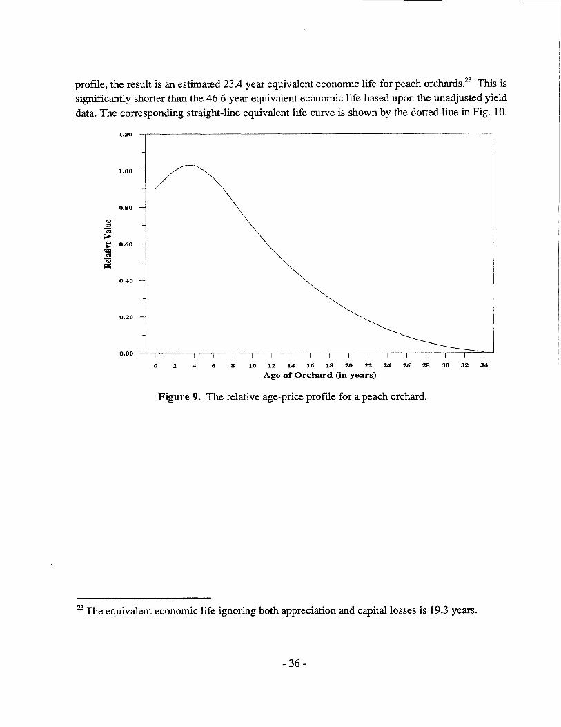
Table 9 presents this data (adjusted for imputed land rent that is assumed to be 15% of the largest annual yield) in the column labelled "relative yield". The relative yield declines only slightly during most of the life of the peach tree in contrast to the much more rapid pattern of decline as described by the experts noted in Appendix B. There may be two reasons for this slow decline. First, the yields are for acreage planted in different locations at each age. It may be that earlier plantings were at more favorable locations, leading to more productive trees. Second, experts may have also considered the decline in the quality of the fruit as the trees age. It is thus assumed that peach yields fall at a declining balance rate after peak yield (which is assumed to occur in the sixth year of the useful life of the trees). The resulting relative yield (again corrected for an imputed land rent) is shown in Table 9 in the column labelled "adjusted relative yield". The age-price profde derived from this yield is shown in Fig. 9.

Table 9. Relative Yield bv Year of C eful Life o a Peach Orchard Adjusted Year of Relative AdjustedRelative Useful Yield Relative

Life Yield Life Yield 0.62 23 I 0.79 0.22

2 0.56 0.60 13 0.89 0.57 0.19 3 0.74 0.78 14 0.93 0.53 0.17 4 0.88 0.92 15 0.92 0.48 0.15 5 0.94 0.97 16 0.90 0.44 0.13 6 0.98 1.00 17 0.88 0.40 0.11 7 1.00 0.93 18 0.87 0.37 q-+0.09 8 0.99 0.86 19 0.84 0.33 0.74 0.07 9 0.93 0.79 20 0.79 0.30 0.06 10 0.90 0.73 21 0.77 0.27 0.04 11 I 0.87 I 0.68 11 22 I 0.76 0.24

Given the distribution of useful lives for cling peach trees, the mean useful life of 16 years derived in Chapter 3, and the relative age-priceprofile shown in Fig. 9, the average relative age-price profile can be derived in the samemanner as for orange trees in SectionA above. If the appreciation in the early years is ignored, the average relative age-price profile noted by the solid line in Fig. 10 is obtained. When the equivalent economic life formula (Equation 1in Chapter 4)is applied to this

- 35 -

a2

profile, the result is an estimated 23.4 year equivalent economic life for peach orchards.= This is significantly shorter than the 46.6 year equivalent economic life based upon the unadjusted yield data. The corresponding straight-line equivalent life curve is shown by the dotted line in Fig. 10.

1.20

1-00

0.80

-3 E=" .--p 0.60

m _I

2 0.40

0.20

0.00

0 2 4 6 8 1 0 1 2 1 4 1 6 1 8 2 0 2 2 2 4 2 6 2 8 3 0 3 2 3 4

Age of Orchard (in years)

Figure 9. The relative age-price profile for a peach orchard.

23 The equivalent economic life ignoring both appreciation and capital losses is 19.3 years.

- 36 -

0 5 10 15 20 25 30 35


Figure 10. The average relative age-price profile for a peach orchard when appreciation is ignored (solid line), and its straight-line equivalent economic life (dotted line).

C. The Equivalent Ekonomic Life of Almond Trees Informationpertaining to the first 10years of yield for a typical acre of California almond trees

has been obtained from expertsz4.This information has been extrapolated by the generic pattern of decline. The resulting relative yield is shown in Table 10. The relative age-price profile is shown in Fig. 11. Given the distribution of useful lives for cling peach trees, the mean useful life of 37 years derived in Chapter 3, and the age-priceprofile shown in Fig. 11,the average relative age-price profile for almond trees can be obtained.

24 The first 7 years of yield are from an unpublished note, "Estimated Non-Discounted Cost of ReplacingAn Almond Tree,April, 1985"by Wesley K. Ask, University of California Farm Advisor for Stanislau County. Other experts suggested that the 7th-10th year's yield represents the peak yield.

- 37 -

1

2

3 4 5 6 7

8

9 10 11 12 13 14

15 16 17

18 19 20 21

22 23 24 25

Table 10. Relative Year of Relative Useful Yield Life

0.06 0.41 0.71 1.oo 1.00 1.oo 1.00 1.00 1.oo 1.oo 1.00 0.97 0.94 0.91 0.88 0.85 0.82 0.79 0.77 0.74 0.72 0.69 0.67 0.65 0.63

Yield by Year of Useful Life of an Almond Orchard Year of Relative Year of Relative

Useful Life Yield Useful Life Yield

26 0.60 51 0.22 27 0.58 52 0.21

28 0.56 53 0.20 29 0.54 54 0.19 30 0.52 55 0.18 31 0.50 56 0.17 32 0.49 57 0.16 33 0.47 58 0.15 34 0.45 59 0.14 35 0.43 60 0.13 36 0.42 61 0.12 37 0.40 62 0.11 38 0.38 63 0.11 39 0.37 64 0.10 40 0.36 65 0.09 41 0.34 66 0.08 42 0.33 67 0.08 43 0.31 68 0.07 44 0.30 69 0.06 45 0.29 70 0.06 46 0.27 71 0.05 47 0.26 72 0.04 48 0.25 73 0.04 49 0.24 74 0.03 50 0.23

-38 -

If the appreciation in the early years is ignored, the average age-price profile noted by the solid line in Fig. 12 is obtained. When the equivalent economic life formula (Equation 1 in Chapter 4) is applied to this profile, the result is an estimated 61.9 year equivalent economic life for almond trees.25 The corresponding straight-line equivalent life curve is shown by the dotted line in Fig. 12.

1.20

0 4 8 12 16 20 24 28 32 36 40 44 A8 52 56 60 64 68 72 76


Figure 11. The relative age-price profile for an almond orchard.


- 39 -

W

1.2

I1

0.8

-s $

0.6 ..-) .--m

I2 0.4

0.2

0

0 5 10 15 20 25 30 35 40 45 50 55 60 65 70


Figure 12. The average relative age-price profile for an almond orchard when appreciation is ignored (solid line), and its straight-line equivalent economic life (dotted line).

ic Life of Ot In this section the equivalent economic life of several tree types are estimated from the useful

lives obtained from Califomia acreage data, the cling peach retirement distribution, and a generic yield curve. The generic yield cuve is obtained by assuming that: 1) the yield in the first year of the useful life is 50% of the peak yield; 2) the yield increases linearly until it reaches peak yield, which occurs when the trees reach an age that is one-third of the useful life; 3) the yield declines from its peak in a declining balance pattern until alI trees stop bearing, which occurs at an age that is twice the useful life26;4)imputed land rent is 15% of peak yield. This is assumed to be the pattem of yield of an acre of h i t and nut trees in the absence of retirements. Table 11presents the relative yield for apple trees (which have a 33 year useful life) based on these assumptions.

26Thedeclining balance pattem is an exponential decline at a rate that is the inverse of the useful life, so that the declining balance rate for apples which have a 33 year useful life would be 1/33 or 3%.

-40-

1 0.41 23 0.66 45 0.25

0.47 24 0.64 46 0.24

3 0.52

4 0.57 26 0.59 48 0.21

0.63 27 0.57 49 0.20

6 0.68 28 0.54 50 0.19

0.73 29 0.52 51 0.18

0.61

Year of Relative Useful Life Yield

Year of Relative Year of Relative Useful Life Yield Useful Life Yield

0.22

1

2

3

4

5

6

7

8 0.79

9 0.84

10 0.89

11 0.95

12 1 .oo 13 0.96

14 0.93

0.90 15

16 0.86

17 0.83

18 0.80

19 0.77

20 0.74

21 0.72

22 0.69

25 47

30 0.50 52 0.17

31 0.48 53 0.16

32 0.46 54 0.15

33 0.44 55 0.14

34 0.42 56 0.13

35 0.40 57 0.12

36 0.39 58 0.1 1

37 0.37 59 0.10

38 0.35 60 0.09

39 0.34 61 0.08

40 0.32 62 0.08

41 0.3 1 63 0.07

42 0.29 64 0.06

43 0.28 65 0.05

44 0.26 66 0.05

8

9

10

11

2

5

7

As mentioned in the introduction to this Chapter, the equivalent economic life estimated using the productivity method is very sensitive to the pattem of yields over the useful life of the trees. The assumption that yields increase over the first third of the useful life is based upon evidence for orange, almond and peach trees and on discussions with experts reported in Appendix B. The rate at which yields decrease is chosen so that when trees reach twice the useful life yield is about 20% of the peak yield (before the 15%reduction for imputed land rents). The generic decline in yield is intended to take into consideration the decline in age with both the volume of h i t and nuts produced and their quality.

Year of Relative Year of Relative Year of Relative Useful Life Yield Useful Life Yield Useful Life Yield

0.41 23 0.66 45 0.25

I 0.47 24 0.64 46 0.24

III1 I ,I 1 II

0.57 26 0.59 48 0.21

I 0.63 27 0.57 49 0.20

0.68 28 0.54 50 0.19

I 0.73 29 0.52 51 0.18

0.79 30 0.50 52 0.17

0.84 31 0.48 53 0.16

0.89 32 0.46 54 0.15 11 I 1 I t

0.95 33 0.44 55 0.14

1.oo 34 0.42 56 0.13

13 0.96 35 0.40 57 0.12

14 0.93 36 0.39 58 0.1 1

15 0.90 37 0.37 59 0.10

I 0.52 II 25 I 0.61 II 47 I 0.22

I ~ ~ ~~~ ~~ ~ ~

16 0.86 38 0.35 60 0.09

17 0.83 39 0.34 61 0.08

18 0.80 40 0.32 62 0.08

19 0.77 41 0.3 1 63 0.07

20 0.74 42 0.29 64 0.06

21 0.72 43 0.28 65 0.05

22 0.69 44 0.26 66 0.05

-41 -

Fig. 13 shows the relative age-price profile for apple trees derived from the generic yield pattern and the 33 year useful life of apple trees. Note that the relative age-price profile for apple trees is similar to that of orange and almond trees. Given the distribution of useful lives for cling peach trees, the relative age-price profile shown in Fig. 13, and the 33 year mean useful life, the average relative age-price profile can be obtained. If the appreciation in the early years is ignored, the average age-price profile noted by the solid line in Fig. 14 is obtained. Applying the equivalent economic life formula to this profile results in a 70.1 year useful life for apple trees.27 The corresponding straight-line equivalent life curve is shown by the dotted line in Fig. 14.

1.20

1.00

0.80

W3 _. s -p 0.60.-.I) cu

2 0.40

0.20

0.00

0 3 6 9 12 15 18 21 24 27 30 33 36 39 42 45 48 51 54 SI 60 63 66 69 72


Figure 13. The relative age-price profile for an apple orchard.


- 4 2 -

1.2

0 5 10 15 20 25 30 35 40 45 50 55 60 65 70 75


Figure 14. The average relative age-price profile for an apple orchard when appreciation is ignored (solid line), and its straight-line equivalent economic life curve (dotted line).

This same generic yield curve and the cling peach survivor curve have been applied to the useful lives (derived from California acreage data) of six other tree types. These are listed in Table 12. It should be noted that the preproductive period plays no role in determining the equivalent economic life of the trees. Apple trees, which have a seven year preproductive period but a 33 year useful life, and English walnut trees which have a four year preproductive period but a 33 year useful life, have the same 70.1 year equivalent economic life.

- 43 -

Table 12. Useful Lives and Equivalent Economic Lives of Fruit and Nut Trees

Tree Useful Life Equivalent Economic Life

Orange

Peach Almond

Apple Grapefruit

English Walnut Plum Prune Lemon Average 28

31.0 67.1 16.0 23.4 37.0 61.9 33.0 70.1 35.0 68.5 33.0 70.1 18.0 33.0 20.0 37.1 22.0 40.1 30.7 61.2

The useful lives shown in Table 12 range from 16 years for peach trees to 37 years for almond trees?’ The equivalent economiclives range from 23.4years for peach trees to 70.1 years for apple and walnut trees. The average useful life of fruit and nut trees obtained by weighting together the useful life entries inTable 12by the acreage (shown in Table 1) is 30.7 years. The averageequivalent economic life of fruit and nut trees also weighted by acreage, is 61.2 years.30

28 The average lives are weighted averages of the lives for the trees that are shown in this table. The weights used for this calculation are the acreage values shown in Table 1. 29 The 16 year useful life for peaches noted here is derived from California acreage data, and is for both cling and freestone peaches. It differs from the 15.1 year useful life for cling peaches alone, as derived from the retirement frequencies in Chapter 3. 30 The average equivalent economic life ignoring both appreciation and capital losses claimed on the retirement of the block, is 42.8 years.

-44-

Chapter 6. Conclusion Fruit and nut trees generally appreciate in value in the early years of the their useful lives.

When applying the equivalenteconomiclife formulato appreciatingassets, it is reasonableto ignore such appreciation, but to take the losses claimed at retirement into account. When this is done, the weighted average equivalent economic life of fruit and nut trees (as measured by the 9 tree types included in Table 12) is 61.2 years, almost twice the acreage weighted average useful life of 30.7 years.

The information collected by the Depreciation Analysis Division indicates that useful lives vary significantly among tree types and by location of the block. The useful lives (and the correspondingequivalent economiclives) estimated in this report are derivedfrom the California acreage data, which although historically accurate,may not be representativeof trees located on other States, or grown using newer horticultural practices. It is primarily the unavailability of data for states other than California or data reflecting more current conditionsthat leads the DepreciationAnalysis Division to merely transmit its findings to Congress without specific recommendation of a class life. However, even if the future average useful life of fruit and nut trees should, for example, decline to 18 years (that reported for plum trees) from the historically measured 31 years, the resulting equivalent economic life may well be comparable to the 33 years given in Table 12 for plums.

- 4 5 -

References

Brazell, David W., Dworin, Lowell, and Walsh, Michael. A History of Federal Tax Depreciation Policy. OTA Paper 64, May 1989, Department of the Treasury.

"California Fruit and Nut Tree Acreage", California Agricultural Statistics Service, 1937-1988.

Childers, Norman. Modern Fruit Science. 1983, Horticultural Publications.

"Florida Citrus Inventory", Florida Agricultural Statistics Service, Published in even numbered years 1966-1988.

Grant Eugene L., and Norton, Paul T. Depreciation. 1955, The Ronald Press Company.

Muraro,Ronald P., and Fairchild,Gary F. "EconomicFactorsAffectingPostfreeze Production Decisions in The Florida Citrus Industry." Proceedings of the Florida State Horticultural Society 98: 1985,pp. 65-70.

"Orchard and Production Survey 1987-1988." 1988,California Cling Peach Advisory Board.

Report to Congress on The Depreciation of Clothing Held for Rental, Department of the Treasury, August, 1989.

"The Cost of Producing California-ArizonaNavelsFor The 1984-1985Season". Cooperative Extension Service, University of California, and Department of Agricultural Economics, University of Arizona. December, 1985.

-47-

Appendix A. Exhibits Related to the Congressional Mandate

Exhibit 1. Section 168(i)(l)(B) of the Internal Revenue Code as Revised by the Tax Reform Act of 1986

Code Sec. 168 (i) Definitions and Special Rules.

For purposes of this section-

(1) Class Life.

(B) Secretarial authority. The Secretary, through an office established in the Treasury-

(i) shall monitor and analyze actual experience with respect to all depreciable assets, and

(ii)except in the case of residential rental property or nonresidential real property-

(I)may prescribe a new class life for any property,

(11) in the case of assigned property, may modify any assigned item, or

(III) may prescribe a class life for any property which does not have a class life within the meaning of subparagraph (A).

Any class life or assigned item prescribed or modified under the preceding sentence shall reasonably reflect the anticipated useful life, and the anticipated decline in value over time, of the property to the industry or other group.

Exhibit 2. Section 168(i)(l) of the Internal Revenue Code as Revised by the Technical and Miscellaneous Revenue Act of 1988:

Code Sec. l68(i) Definitions and Special Rules.

For purposes of this section-

(1) Class Life. Except as provided in this section, the term "class life" means the class life (if any) which would be applicable with respect to any property as of January 1, 1986,under subsection (m) of section 167 (determined without regard to paragraph (4) and as if the taxpayer had made an election under such subsection). The Secretary, through an office established in the Treasury, shall monitor and analyze actual experience with respect to all depreciable assets.

-49-

The Secretary, through an office established in the Treasury Department is authorized to monitor and analyze actual experience with all tangible depreciable assets, to prescribe a new class life for any property or class of property (otherthan real property) when appropriate, and to prescribe a class life for any property that does not have a class life. If the Secretary prescribes a new class life for property, such life will be used in determining the classification of property. Theprescription of a new class life for property will not change the ACRS class structure, but will affect the ACKS class in which the property falls. Any classification or reclassification would be prospective.

Any class life prescribed under the Secretary's authority must reflect the anticipated useful life, and the anticipated decline in value over time, of an asset to the industry or other group. Useful life means the economic life span of property over all users combined and not, as under prior law, the typical period over which a taxpayer holds the property. Evidence indicative of the useful life of property, which the Secretary is expected to take into account in prescribing a class life, includes the depreciation practices followed by taxpayers for book purposes with respect to the property, and useful lives experienced by taxpayers, according to their reports. It further includes independent evidence of "Iuseful life -- the terms for which new property is leased, used under a service contract, or financed -- and independent evidence of the decline in value of an asset over time, such as is afforded by resale price data. If resale price data is used to prescribe class lives, such resale price data should be adjusted downwardto removetheeffects of historical inflation. Thisadjustment provides a larger measure of depreciation than in the absence of such an adjustment. Class lives using this data would be determined such that the present value of straight-line depreciation deductions over the class life, discounted at an appropriate real rate of interest, is equal to the present value of what the estimated decline in value of the asset would be in the absence of inflation.

Initial studies are expected to concentrate on property that now has no ADR midpoint. Additionally, clothing held for rental and scientific instruments (especially those used in connection with a computer) should be studied to determine whether a change in class life is appropriate.

Certain other assets specifically assigned a recovery period (including horses in the three-year class, qualified technological equipment, computer-based central office switching equipment, research and experimentation property, certain renewable energy and biomass properties, semi-conductor manufacturing equipment, railroad track, single-purpose agricultural or horticultural structures,telephone distributionplant and comparable equipment, municipal waste-water treatment plants, and municipal sewers) may not be assigned a longer class life by the Treasury Department if placed in service before January 1,1992. Additionally, automobiles and light trucks may not be reclassified by the Treasury Department during this five-year period. Such property placed in service after December 31, 1991, and before July 1, 1992, may be prescribed a different class life

- 50 -

if the Secretary has notified the Committee on Ways and Means of the House of Representatives and the Committee on Finance of the Senate of the proposed change at least 6 months before the date an which such change is to take effect.

- 5 1 -

Appendix B. Meetings with Fruit and Nut Tree Growers and Other Experts Members of DAD visited California and Florida in order to seek expert opinions concerning

the depreciation of fruit and nut trees. DAD staff met with experts who grow trees, work for agricultural agencies, are affiliated with agricultural schools, and work for corporations engaged in farming various tree crops. This appendix contains a list of the visits with these experts.

The first section of the appendix contains a list of the meetings during the Florida visit which occurred in October, 1988 and consisted entirely of meetings with citrus tree experts. The second section of this appendix contains a list of meetings with experts on California fruit and nut trees. The California visit occurred in November, 1988.

Exhibit 1. Meetings With Florida Citrus Growers and Experts Driving Tour Through Citrus Growing Areas Between Orlando and Lake Alfred.

Expert: Edd Dean, Vice President and Controller of Florida Citrus Mutual

Meeting With Growers, Agricultural Experts, and CPA’s at the Citrus Experiment Station in Lake Alfred.

Experts: Edd Dean, Bobby F. McKown, Florida Citrus Mutual; Atlee Harmon, Johnnie Jarnes, Peat Marwick; Phil Hemdan, Alcoma; Martin J. McKenna, Joe L. Davis Groves Tnc.; Ron Muraro, David Tucker, CREC-IFAS; J. S. Parrish ITI, Nevins Fruit Co. Inc.. Thomas Riffle, Rex McPherson, Lake Butler Groves, Tnc.; Dean Saunders, Sen. Lawton Chiles’ Office; Tom Taylor, Steve Southard, Berry Groves Inc. Glenn Thomas, Orange County; Bob Turner, Citrus World Inc.

Drive from Lakeland to 1,aBelle and a Visit to a Grove Owned by the Berry Corporation near Labelle.

Experts: Edd Dean, Florida Citrus Mutual; Herb Pollard, Berry Corporation;

Visit to Alico Corporation in Labelle

Experts: Dr. Bernie kster, an economist working for Alico; Mr. Junior Merritt, an Alico employee

Drive from Labelle to Ft. Pierce; Breakfast at Fort Pierce; and visit to the Strazzula Grove near Fort Pierce

- 53 -

Experts: Edd Dean, Florida Citrus Mutual; Michael Minton, Florida Bar ‘Tax Section; John David Smith, an accountant knowledgeable in citrus

accounting who works for Graves Brothers, citrus growers; Phil Strazzula, a citrus grower

Flight over Groves in St. Eucie and Martin Counties

Expert: Brantly Sherrard of Blue Goose Corporation

Visit to the Minton Packinghouse and Groves

Expert: Michael Minton, owner

Visit to the Sciotto Family Grove

Experts: Michael Minton, owner, Minton Packinghouse; Dominic Sciotto, owner, Sciotto family grove

Meeting at the S Agricultural Research and Education Center in Ft. Pierce.

Experts: Dr.Ron Bowman, irrigation expert; Dr. David Calvert, a soil chemist and Director of the IFAS Center;

Dr. Ronald Sonoda, citrus pathologist

d Nut Tree Growers and Experts

California Orange Growers in the Vicinity of Visalia, California.

Experts: Members of the California Citrus Mutual Joel Nelson, California Citrus Mutual Bob Wade, grove owner Guy Wollenman, owner of Wollen” Farms

Meeting with California Apricot Growers at the Offices of the Apricot Producers of California in Modesto, California

Experts: Lauren Campbell, an apricot grower, board member of the Aricot Producers of California (APC),and member of the California Apricot Advisory Board; Frank Mosebar, Dried Fruit Association of California; Les Rose, Vice President of Operations for the APC

- 54 -

Meeting with Walnut Growers at Diamond Walnut Growers in Stockton, Calm ifornia Experts: Gerald Barton, Grower and President of Diamond Walnut Growers, Inc.;

Tom Ciccarelli, Grower; Robert C. Estes, Accountant at Touche Ross & Co.; Bill Gillis, Vice President and Chief Administrative Officer of Diamond Walnut Growers, hc.; Joe Grant, San Joaquin County FarmAdvisor, University of California Cooperative Extension. Kathy Kelley, Stanislaus County Farm Advisor, IJniversity of California Cooperative Extension; Bob Merrill of Diamond Walnut Growers, Inc.; John Repanich, Grower and Diamond Walnut Grower Director; Bill Waggershauser, Grower and Diamond Walnut Growers Director;

Meetings with California Olive Growers In and Around Lindsay, California Experts: Bob Rossio, President of Lindsay Olive Growers, a cooperative; Earl Kinsel, Lindsay

Olive Growers; Greg Childress, grower from the southem portion of the California olive growing region; Bob Shawl, grower from the central portion of the California olive growing region; Lawrence Aguira, grower from the northem portion of the California olive growing region

Meeting with California Peach Growers at the California Canning Peach Association Modesto Offices Experts: Randy Fiorini, Grower

Howard F. Gingerich, California Cling Peach Advisory Board (CCPAB); Pete Grubeck, Grower Ron Martella, Grower Jon Murphy of the California Canning Peach Association (CCPA); Ron Schuler of the CCPA; George Tavernas, Grower

Meeting with California Pear Growers at the California Pear Growers Fall 1988 District Meetings held at the Ryde Hotel in Ryde, California Experts: Jean-Marie Peltier of the California Pear Growers

Association (CPGA);

- 55 -

Greg Vogel, Sacramento County Farm Advisor; an accountant familiar with fann accounting; several growers; two extension service agents

Experts: Tom Johnson, foreman of The West Hills Almond Cooperative Mike Neal, The Blackwell Land Company,

California Pistachio Growers in Washington DC Experts: Bob Schrarrmi California Pistachio Commission

Growers, Members of the California Pistachio Commission

- 56 -

Acknowledgements This report was prepared by Lowell Dworin and Gerald Silverstein from data obtained by William Strang, who also developed the preliminary analysis. Secretarialassistance wasprovided by Carolyn Greene.

- 57 -

treasury report on the depreciation of fruit and nut … the depreciation of fruit and nut trees...

Documents