treasury presentation to tbac - united states … of treasury’s february 2017 quarterly refunding...

Treasury Presentation to TBAC

Office of Debt Management

Fiscal Year 2017 Q1 Report

Table of Contents

2

I. Executive Summary p. 4

II. Fiscal A. Quarterly Tax Receipts p. 6 B. Monthly Receipt Levels p. 7 C. Eleven Largest Outlays p. 8 D. Treasury Net Nonmarketable Borrowing p. 9 E. Cumulative Budget Deficits p. 10 F. Deficit and Borrowing Estimates p. 11 G. Budget Surplus/Deficit p. 12

III. Financing A. Sources of Financing p. 15 B. OMB’s Projections of Net Borrowing from the Public p. 17 C. Interest Rate Assumptions p. 18 D. Net Marketable Borrowing on “Auto Pilot” Versus Deficit Forecasts p. 19

IV. Portfolio Metrics A. Weighted Average Maturity of Marketable Debt Outstanding with Projections p. 24 B. Maturity Profile p. 25

V. Demand A. Summary Statistics p. 30 B. Bid-to-Cover Ratios p. 31 C. Investor Class Awards at Auction p. 36 D. Primary Dealer Awards at Auction p. 40 E. Direct Bidder Awards at Auction p. 41 F. Foreign Awards at Auction p. 42

Section I: Executive Summary

3

Receipts and Outlays • Fiscal year-to-date receipts are $25 billion lower than the same period of the previous year, due mainly to a decrease in Federal Reserve

Earnings. (In December 2015, FAST Act Legislation resulted in a one-time transfer of $19 billion from the Federal Reserve System to the Treasury.)

• In Q1 FY 2017, outlays were lower in most categories than in the same period of the previous year. After adjusting for calendar differences, however, year-over-year budget outlays were 3 percent higher.

• The main driver behind the growth in outlays were an increase in interest expense (+$15 billion) and HHS expenditures (+$14 billion).

Sources of Financing in Fiscal Year 2017 • Based on the Quarterly Borrowing Estimate, Treasury’s Office of Fiscal Projections currently projects a net marketable borrowing need

of $57 billion for Q2 FY 2017, with an end of March cash balance of $100 billion. For Q3 FY 2017, net marketable borrowing need is projected to be $1 billion, with an end of June cash balance of $200 billion.

Projected Net Marketable Borrowing

• Between FY 2017 and 2019 Treasury’s net marketable borrowing could rise notably if the Federal Reserve allows the Treasury securities held in the SOMA portfolio to mature without reinvesting.

• As of the December 2016 Survey of Primary Dealers, the median expectation was for SOMA reinvestments to continue until June 2018.

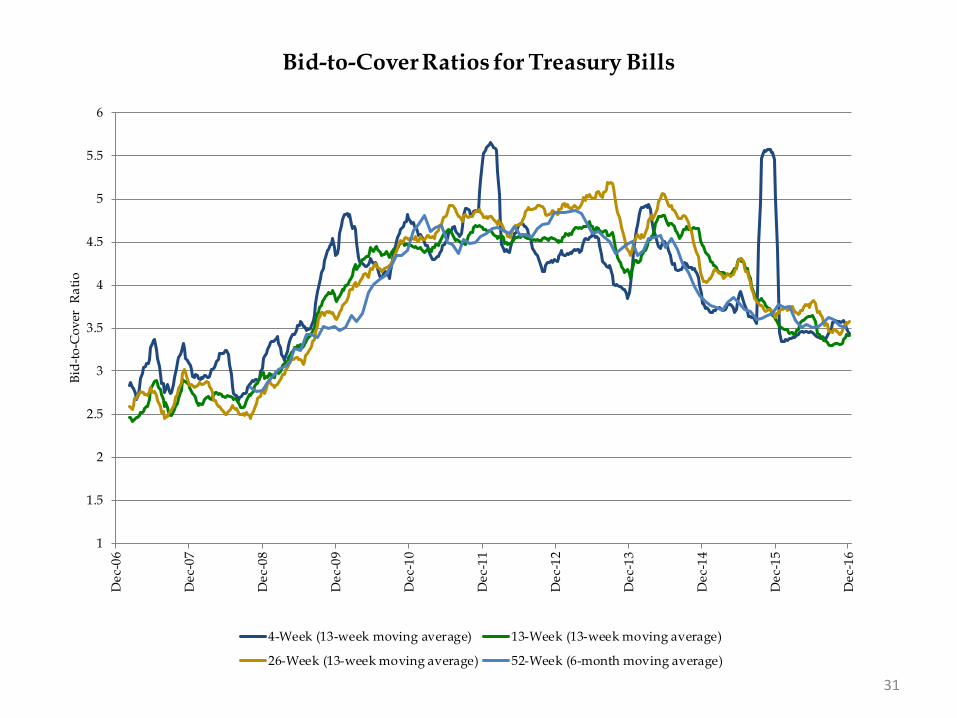
Bid-to-Cover Ratios (BTC) • Since October, BTC ratios for 10-year coupon securities have fallen slightly. • BTC ratios for all other securities were stable over the October to December period.

Investor Class Allotments

• Since mid-2016, bill auction awards have been trending higher for investment funds and largely stable for other dealers and brokers and international institutions. Accordingly, bill auction awards fell for primary dealers.

• Over the same period, coupon auction awards were higher for primary dealers, lower for international institutions and largely stable for other investors.

Highlights of Treasury’s February 2017 Quarterly Refunding Presentation to the Treasury Borrowing Advisory Committee (TBAC)

4

Section II: Fiscal

5

6 Source: United States Department of the Treasury

(50%)

(40%)

(30%)

(20%)

(10%)

0%

10%

20%

30%

40%

50%

60%

Dec

-06

Apr

-07

Aug

-07

Dec

-07

Apr

-08

Aug

-08

Dec

-08

Apr

-09

Aug

-09

Dec

-09

Apr

-10

Aug

-10

Dec

-10

Apr

-11

Aug

-11

Dec

-11

Apr

-12

Aug

-12

Dec

-12

Apr

-13

Aug

-13

Dec

-13

Apr

-14

Aug

-14

Dec

-14

Apr

-15

Aug

-15

Dec

-15

Apr

-16

Aug

-16

Dec

-16

Yea

r-ov

er-Y

ear

% C

hang

eQuarterly Tax Receipts

Corporate Taxes Non-Withheld Taxes (incl SECA) Withheld Taxes (incl FICA)

7 Individual Income Taxes include withheld and non-withheld. Social Insurance Taxes include FICA, SECA, RRTA, UTF deposits, FUTA and RUIA. Other includes excise taxes, estate and gift taxes, customs duties and miscellaneous receipts. Source: United States Department of the Treasury

0

20

40

60

80

100

120

140

Dec

-06

Apr

-07

Aug

-07

Dec

-07

Apr

-08

Aug

-08

Dec

-08

Apr

-09

Aug

-09

Dec

-09

Apr

-10

Aug

-10

Dec

-10

Apr

-11

Aug

-11

Dec

-11

Apr

-12

Aug

-12

Dec

-12

Apr

-13

Aug

-13

Dec

-13

Apr

-14

Aug

-14

Dec

-14

Apr

-15

Aug

-15

Dec

-15

Apr

-16

Aug

-16

Dec

-16

$ bn

Monthly Receipt Levels(12-Month Moving Average)

Individual Income Taxes Corporation Income Taxes Social Insurance Taxes Other


0

50

100

150

200

250

300

HH

S

SSA

Def

ense

Trea

sury

Agr

icul

ture

Labo

r

VA

Tran

spor

tatio

n

OP

M

Educ

atio

n

Oth

er D

efen

se C

ivil

$ bn

Eleven Largest Outlays

Oct - Dec FY 2016 Oct - Dec FY 2017


(40)

(30)

(20)

(10)

0

10

20

30

Q1-

07Q

2-07

Q3-

07Q

4-07

Q1-

08Q

2-08

Q3-

08Q

4-08

Q1-

09Q

2-09

Q3-

09Q

4-09

Q1-

10Q

2-10

Q3-

10Q

4-10

Q1-

11Q

2-11

Q3-

11Q

4-11

Q1-

12Q

2-12

Q3-

12Q

4-12

Q1-

13Q

2-13

Q3-

13Q

4-13

Q1-

14Q

2-14

Q3-

14Q

4-14

Q1-

15Q

2-15

Q3-

15Q

4-15

Q1-

16Q

2-16

Q3-

16Q

4-16

Q1-

17

$ bn

Fiscal Quarter

Treasury Net Nonmarketable Borrowing

Foreign Series State and Local Govt. Series (SLGS) Savings Bonds


0

100

200

300

400

500

600

700

Oct

ober

Nov

embe

r

Dec

embe

r

Janu

ary

Febr

uary

Mar

ch

Apr

il

May

June

July

Aug

ust

Sept

embe

r

$ bn

Cumulative Budget Deficits by Fiscal Year

FY2015 FY2016 FY2017

11

FY 2017-2019 Deficits and Net Marketable Borrowing Estimates In $ billionsPrimary Dealers1 CBO2 CBO3 OMB MSR4 OMB5

FY 2017 Deficit Estimate 661 559 433 441 504FY 2018 Deficit Estimate 771 487 383 330 454FY 2019 Deficit Estimate 863 601 518 427 550FY 2017 Deficit Range 525-1010FY 2018 Deficit Range 587-1035FY 2019 Deficit Range 690-1200

FY 2017 Net Marketable Borrowing Estimate 699 670 508 573 635FY 2018 Net Marketable Borrowing Estimate 837 578 452 436 561FY 2019 Net Marketable Borrowing Estimate 927 676 578 534 659FY 2017 Net Marketable Borrowing Range 535-1160FY 2018 Net Marketable Borrowing Range 540-1185FY 2019 Net Marketable Borrowing Range 700-1250Estimates as of: Jan-17 Jan-17 Mar-16 Jul-16 Feb-16

1Based on primary dealer feedback on January 23, 2017. Estimates above are averages. 2Summary Table 1 of CBO's "The Budget and Economic Outlook: 2017 to 2027"3Table 1 and 2 of CBO's "An Analysis of the President's 2017 Budget"4Table S-11 of OMB's “The FY2017 Mid-Session Review” 5Table S-13 of OMB's “Budget of the United States Government, Fiscal Year 2017”

(12%)

(10%)

(8%)

(6%)

(4%)

(2%)

0%

(1,600)

(1,400)

(1,200)

(1,000)

(800)

(600)

(400)

(200)

0

2007

2008

2009

2010

2011

2012

2013

2014

2015

2016

2017

2018

2019

2020

2021

2022

2023

2024

2025

2026

% o

f GD

P

$ bn

Fiscal Year

Budget Surplus/Deficit

Surplus/Deficit (LHS) Surplus/Deficit (RHS)

Projections are from Table S-11 of “The FY2017 Mid-Session Review.” 12

OMB’s Projection

Section III: Financing

13

14

Assumptions for Financing Section (pages 15 to 22)

• Portfolio and SOMA holdings as of 12/31/2016. • SOMA reinvestments until June 2018, followed by SOMA redemptions until and including February

2022. These assumptions are based on Chair Yellen’s December 2015 press conference and the median expectations from the December 2016 FRB-NY Survey of Primary Dealers.

• Assumes announced issuance sizes and patterns constant for Nominal Coupons, TIPS, and FRNs as of 12/31/2016, while using an average of ~$1.8 trillion of Bills outstanding.

• The principal on the TIPS securities was accreted to each projection date based on market ZCIS levels as of 12/31/2016.

• No attempt was made to match future financing needs.

15

Sources of Financing in Fiscal Year 2017 Q1

*An end-of-December 2016 cash balance of $399 billion versus a beginning-of-October 2016 cash balance of $353 billion. By keeping the cash balance constant, Treasury arrives at the net implied funding number. Gross issuance values include SOMA add-ons.

Net Bill Issuance 171 Security Gross Maturing Net Gross Maturing Net

Net Coupon Issuance 84 4-Week 655 610 45 655 610 45

Subtotal: Net Marketable Borrowing 255 13-Week 505 502 3 505 502 3

26-Week 427 328 99 427 328 99

Ending Cash Balance 399 52-Week 60 36 24 60 36 24

Beginning Cash Balance 353 CMBs 0 0 0 0 0 0

Subtotal: Change in Cash Balance 46 Bill Subtotal 1,647 1,476 171 1,647 1,476 171

Net Implied Funding for FY 2017 Q1* 209

Security Gross Maturing Net Gross Maturing Net

2-Year FRN 42 41 1 42 41 1

2-Year 56 57 (1) 56 57 (1)

3-Year 77 90 (13) 77 90 (13)

5-Year 74 73 1 74 73 1

7-Year 61 65 (4) 61 65 (4)

10-Year 68 23 45 68 23 45

30-Year 42 19 23 42 19 23

5-Year TIPS 14 0 14 14 0 14

10-Year TIPS 12 0 12 12 0 12

30-Year TIPS 5 0 5 5 0 5

Coupon Subtotal 452 368 84 452 368 84

Total 2,099 1,844 255 2,099 1,844 255

Coupon Issuance Coupon Issuance

October - December 2016 October - December 2016 Fiscal Year-to-DateBill Issuance Bill Issuance

October - December 2016 Fiscal Year-to-Date

16

Sources of Financing in Fiscal Year 2017 Q2

*Keeping announced issuance sizes and patterns constant for Nominal Coupons, TIPS, and FRNs as of 12/31/2016. **Assumes an end-of-March 2017 cash balance of $100 billion versus a beginning-of-January 2017 cash balance of $399 billion. Financing Estimates released by the Treasury can be found here: http://www.treasury.gov/resource-center/data-chart-center/quarterly-refunding/Pages/Latest.aspx

Assuming Constant Coupon Issuance Sizes*Treasury Announced Net Marketable Borrowing** 57

Net Coupon Issuance 101Implied Change in Bills (44)

Security Gross Maturing Net Gross Maturing Net

2-Year FRN 44 41 3 85 82 3

2-Year 116 105 11 172 162 10

3-Year 76 90 (14) 153 180 (27)

5-Year 152 143 8 225 216 9

7-Year 125 131 (7) 185 196 (11)

10-Year 67 22 45 135 45 89

30-Year 41 0 41 84 19 65

5-Year TIPS 0 0 0 14 0 14

10-Year TIPS 26 21 5 38 21 18

30-Year TIPS 8 0 8 13 0 13

Coupon Subtotal 654 553 101 1,106 921 185

January - March 2017

January - March 2017 Fiscal Year-to-DateCoupon Issuance Coupon Issuance

http://www.treasury.gov/resource-center/data-chart-center/quarterly-refunding/Pages/Latest.aspx










573

436

534 530550

652 667 650739

808

55%

60%

65%

70%

75%

80%

(400)

(200)

0

200

400

600

800

1,000

2017

2018

2019

2020

2021

2022

2023

2024

2025

2026

$ bn

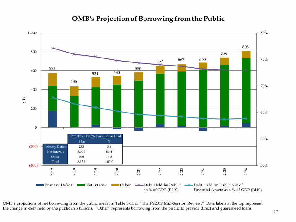
OMB's Projection of Borrowing from the Public

Primary Deficit Net Interest Other Debt Held by Publicas % of GDP (RHS)

Debt Held by Public Net ofFinancial Assets as a % of GDP (RHS)

17

OMB’s projections of net borrowing from the public are from Table S-11 of “The FY2017 Mid-Session Review.” Data labels at the top represent the change in debt held by the public in $ billions. “Other” represents borrowing from the public to provide direct and guaranteed loans.

$ bn %Primary Deficit 233 3.8

Net Interest 5,000 81.4Other 906 14.8Total 6,139 100.0

FY2017 - FY2026 Cumulative Total

18 OMB's economic assumption of the 10-Year Treasury Note rates are from Table S-11 of “The FY2017 Mid-Session Review.” The forward rates are the implied 10-Year Treasury Note rates on December 31 of that year.

1

1.5

2

2.5

3

3.5

4

4.5

2016

2017

2018

2019

2020

2021

2022

2023

2024

2025

2026

10-Y

ear T

reas

ury

Not

e R

ate,

%

Interest Rate Assumptions: 10-Year Treasury Note

OMB FY 2017 MSR Implied Forward Rates as of 12/31/2016

10-Year Treasury Rate of 2.45% as of 12/31/2016

19

Impact of SOMA Actions on Projected Net Borrowing Assuming Future Issuance Remains Constant

Treasury’s primary dealer survey estimates can be found on page 11. OMB's projections of net borrowing from the public are from Table S-11 of “The FY2017 Mid-Session Review.” CBO's estimates of the borrowing from the public are Summary Table 1 of “The Budget and Economic Outlook: 2017 to 2027.” See table at the end of this section for details. *Does not reflect SOMA reinvestments after June 2018 and before February 2022.

0

200

400

600

800

1,000

1,200

1,400

1,600

2017

2018

2019

2020

2021

2022

2023

2024

2025

2026

2027

Fiscal Year

Without Fed Reinvestments ($ bn)*

Projected Net Borrowing

CBO's "The Budget and Economic Outlook: 2017 to 2027"

0

200

400

600

800

1,000

1,200

1,400

1,600

2017

2018

2019

2020

2021

2022

2023

2024

2025

2026

2027

Fiscal Year

With Fed Reinvestments ($ bn)

OMB's FY 2017 Mid-Session Review

PD Survey Marketable Borrowing Estimates

20 Assumes normalization will be complete by FY 2023, which implies no additional funding gap.

0

(106)

(431)

(342)

(227)

(110)

0

(500)

(450)

(400)

(350)

(300)

(250)

(200)

(150)

(100)

(50)

0

50

2017

2018

2019

2020

2021

2022

2023

$ bn

Fiscal Year

Additional Funding Gap Assuming No SOMA Roll after June 2018

21

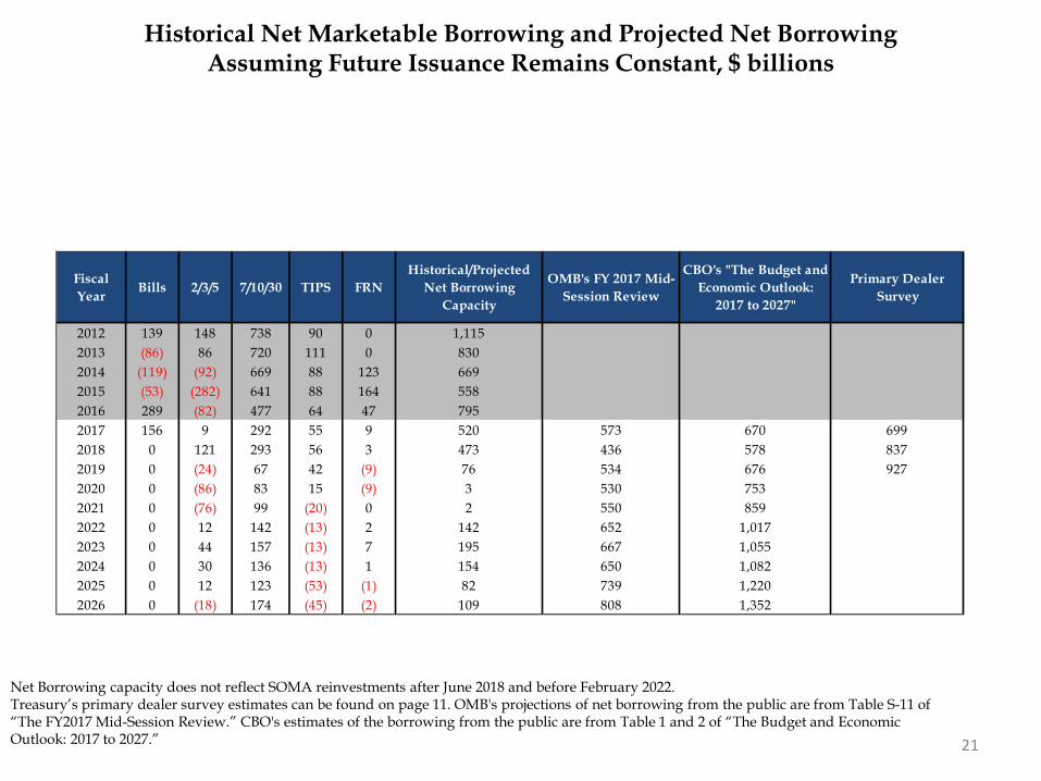
Historical Net Marketable Borrowing and Projected Net Borrowing Assuming Future Issuance Remains Constant, $ billions

Net Borrowing capacity does not reflect SOMA reinvestments after June 2018 and before February 2022. Treasury’s primary dealer survey estimates can be found on page 11. OMB's projections of net borrowing from the public are from Table S-11 of “The FY2017 Mid-Session Review.” CBO's estimates of the borrowing from the public are from Table 1 and 2 of “The Budget and Economic Outlook: 2017 to 2027.”

Fiscal Year Bills 2/3/5 7/10/30 TIPS FRN

Historical/Projected Net Borrowing

Capacity

OMB's FY 2017 Mid-Session Review

CBO's "The Budget and Economic Outlook:

2017 to 2027"

Primary Dealer Survey

2012 139 148 738 90 0 1,115 2013 (86) 86 720 111 0 830 2014 (119) (92) 669 88 123 669 2015 (53) (282) 641 88 164 558 2016 289 (82) 477 64 47 795 2017 156 9 292 55 9 520 573 670 699 2018 0 121 293 56 3 473 436 578 837 2019 0 (24) 67 42 (9) 76 534 676 927 2020 0 (86) 83 15 (9) 3 530 753 2021 0 (76) 99 (20) 0 2 550 859 2022 0 12 142 (13) 2 142 652 1,017 2023 0 44 157 (13) 7 195 667 1,055 2024 0 30 136 (13) 1 154 650 1,082 2025 0 12 123 (53) (1) 82 739 1,220 2026 0 (18) 174 (45) (2) 109 808 1,352

Section IV: Portfolio Metrics

22

23

Assumptions for Portfolio Metrics Section (pages 25 to 30) and Appendix

• Portfolio and SOMA holdings as of 12/31/2016. • SOMA reinvestments until June 2018, followed by SOMA redemptions until and including February

2022. These assumptions are based on Chair Yellen’s December 2015 press conference and the median expectations from the December 2016 FRB-NY Survey of Primary Dealers.

• Assumes announced issuance sizes and patterns constant for Nominal Coupons, TIPS, and FRNs as of 12/31/2016, while using an average of ~$1.8 trillion of Bills outstanding.

• To match OMB’s projected borrowing from the public for the next 10 years, Nominal Coupon securities (2-, 3-, 5-, 7-, 10-, and 30-year) were adjusted by the same percentage.

• The principal on the TIPS securities was accreted to each projection date based on market ZCIS levels as of 12/31/2016.

• OMB’s estimates of borrowing from the public are Table S-11 of the “Fiscal Year 2017 Mid-Session Review.”

24 This scenario does not represent any particular course of action that Treasury is expected to follow. Instead, it is intended to demonstrate the basic trajectory of average maturity absent changes to the mix of securities issued by Treasury.

40

45

50

55

60

65

70

75

80

8519

80

1982

1984

1986

1988

1990

1992

1994

1996

1998

2000

2002

2004

2006

2008

2010

2012

2014

2016

2018

2020

2022

2024

2026

Wei

ghte

d A

vera

ge M

atur

ity (

Mon

ths)

Calendar Year

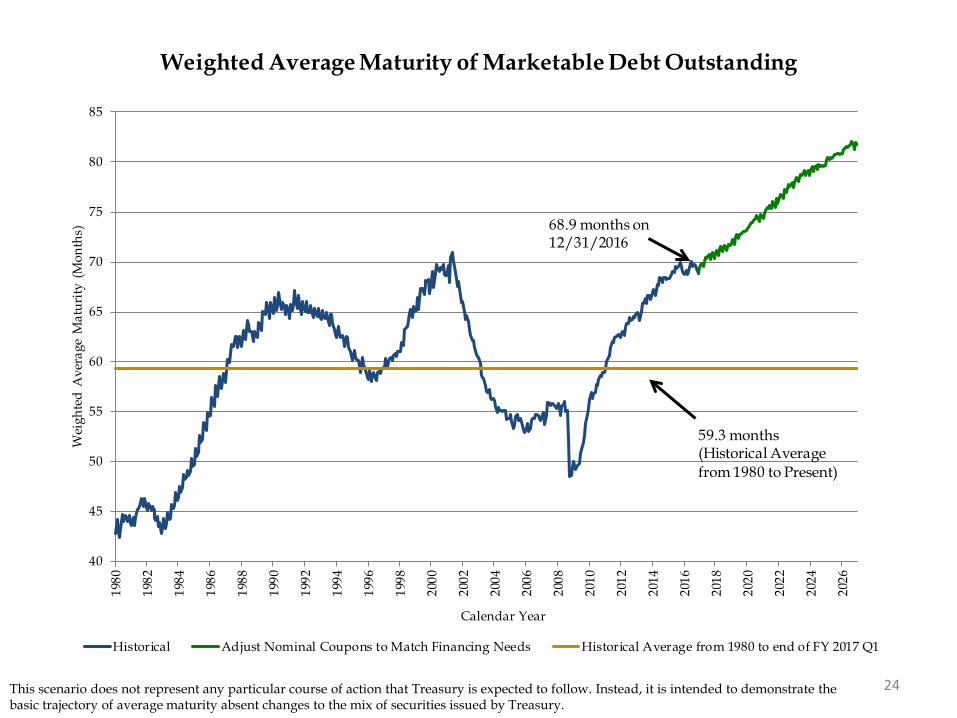
Weighted Average Maturity of Marketable Debt Outstanding

Historical Adjust Nominal Coupons to Match Financing Needs Historical Average from 1980 to end of FY 2017 Q1

68.9 months on12/31/2016

59.3 months(Historical Averagefrom 1980 to Present)

25 This scenario does not represent any particular course of action that Treasury is expected to follow. Instead, it is intended to demonstrate the basic trajectory of average maturity absent changes to the mix of securities issued by Treasury. See table on following page for details.

0

5

10

15

20

25

2017

2018

2019

2020

2021

2022

2023

2024

2025

2026

$ tr

Projected Maturity Profile from end of Fiscal Year

<= 1yr (1,2] (2,3] (3,5] (5,7] (7,10] > 10

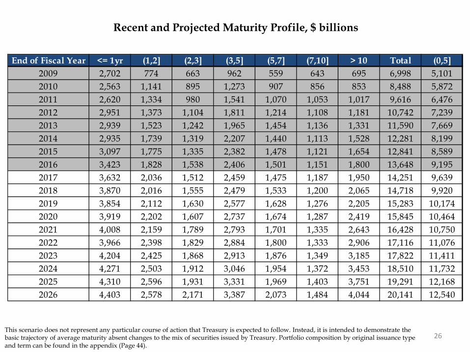
26 This scenario does not represent any particular course of action that Treasury is expected to follow. Instead, it is intended to demonstrate the basic trajectory of average maturity absent changes to the mix of securities issued by Treasury. Portfolio composition by original issuance type and term can be found in the appendix (Page 44).

Recent and Projected Maturity Profile, $ billions

End of Fiscal Year <= 1yr (1,2] (2,3] (3,5] (5,7] (7,10] > 10 Total (0,5]2009 2,702 774 663 962 559 643 695 6,998 5,1012010 2,563 1,141 895 1,273 907 856 853 8,488 5,8722011 2,620 1,334 980 1,541 1,070 1,053 1,017 9,616 6,4762012 2,951 1,373 1,104 1,811 1,214 1,108 1,181 10,742 7,2392013 2,939 1,523 1,242 1,965 1,454 1,136 1,331 11,590 7,6692014 2,935 1,739 1,319 2,207 1,440 1,113 1,528 12,281 8,1992015 3,097 1,775 1,335 2,382 1,478 1,121 1,654 12,841 8,5892016 3,423 1,828 1,538 2,406 1,501 1,151 1,800 13,648 9,1952017 3,632 2,036 1,512 2,459 1,475 1,187 1,950 14,251 9,6392018 3,870 2,016 1,555 2,479 1,533 1,200 2,065 14,718 9,9202019 3,854 2,112 1,630 2,577 1,628 1,276 2,205 15,283 10,1742020 3,919 2,202 1,607 2,737 1,674 1,287 2,419 15,845 10,4642021 4,008 2,159 1,789 2,793 1,701 1,335 2,643 16,428 10,7502022 3,966 2,398 1,829 2,884 1,800 1,333 2,906 17,116 11,0762023 4,204 2,425 1,868 2,913 1,876 1,349 3,185 17,822 11,4112024 4,271 2,503 1,912 3,046 1,954 1,372 3,453 18,510 11,7322025 4,310 2,596 1,931 3,331 1,969 1,403 3,751 19,291 12,1682026 4,403 2,578 2,171 3,387 2,073 1,484 4,044 20,141 12,540


0%

10%

20%

30%

40%

50%

60%

70%

80%

90%

100%

2017

2018

2019

2020

2021

2022

2023

2024

2025

2026

Perc

ent C

ompo

sitio

inProjected Maturity Profile from end of Fiscal Year

<= 1yr (1,2] (2,3] (3,5] (5,7] (7,10] > 10

28

Recent and Projected Maturity Profile, percent

This scenario does not represent any particular course of action that Treasury is expected to follow. Instead, it is intended to demonstrate the basic trajectory of average maturity absent changes to the mix of securities issued by Treasury. Portfolio composition by original issuance type and term can be found in the appendix (Page 44).

End of Fiscal Year <= 1yr (1,2] (2,3] (3,5] (5,7] (7,10] > 10 (0,3] (0,5]2009 38.6 11.1 9.5 13.7 8.0 9.2 9.9 59.1 72.92010 30.2 13.4 10.5 15.0 10.7 10.1 10.0 54.2 69.22011 27.2 13.9 10.2 16.0 11.1 10.9 10.6 51.3 67.32012 27.5 12.8 10.3 16.9 11.3 10.3 11.0 50.5 67.42013 25.4 13.1 10.7 17.0 12.5 9.8 11.5 49.2 66.22014 23.9 14.2 10.7 18.0 11.7 9.1 12.4 48.8 66.82015 24.1 13.8 10.4 18.5 11.5 8.7 12.9 48.3 66.92016 25.1 13.4 11.3 17.6 11.0 8.4 13.2 49.7 67.42017 25.5 14.3 10.6 17.3 10.4 8.3 13.7 50.4 67.62018 26.3 13.7 10.6 16.8 10.4 8.2 14.0 50.6 67.42019 25.2 13.8 10.7 16.9 10.7 8.3 14.4 49.7 66.62020 24.7 13.9 10.1 17.3 10.6 8.1 15.3 48.8 66.02021 24.4 13.1 10.9 17.0 10.4 8.1 16.1 48.4 65.42022 23.2 14.0 10.7 16.8 10.5 7.8 17.0 47.9 64.72023 23.6 13.6 10.5 16.3 10.5 7.6 17.9 47.7 64.02024 23.1 13.5 10.3 16.5 10.6 7.4 18.7 46.9 63.42025 22.3 13.5 10.0 17.3 10.2 7.3 19.4 45.8 63.12026 21.9 12.8 10.8 16.8 10.3 7.4 20.1 45.4 62.3

Section V: Demand

29

30 *Weighted averages of Competitive Awards. **Approximated using prices at settlement and includes both Competitive and Non-Competitive Awards. For TIPS’ 10-year equivalent, a constant auction BEI is used as the inflation assumption.

Summary Statistics for Fiscal Year 2017 Q1 Auctions

Security Type Term Stop Out

Rate (%)*Bid-to-Cover

Ratio*

Competitive Awards

($bn)

% Primary Dealer*

% Direct*

% Indirect*

Non-Competitive Awards ($bn)

SOMA Add Ons

($bn)

10-Year Equivalent

($bn)**

Bill 4-Week 0.333 3.4 649.0 54.4 5.3 40.3 3.9 0.0 5.6Bill 13-Week 0.432 3.4 495.3 59.4 6.0 34.6 5.1 0.0 14.0Bill 26-Week 0.560 3.6 417.2 44.9 2.3 52.8 4.4 0.0 23.7Bill 52-Week 0.735 3.5 59.5 56.6 2.9 40.5 0.5 0.0 6.6

Coupon 2-Year 1.073 2.6 77.5 55.0 10.9 34.1 0.5 7.8 18.9Coupon 3-Year 1.177 2.8 71.9 45.3 8.9 45.8 0.1 5.3 25.3Coupon 5-Year 1.707 2.5 101.9 31.8 4.5 63.6 0.1 10.2 59.8Coupon 7-Year 2.051 2.6 84.0 20.1 13.8 66.0 0.0 8.4 67.1Coupon 10-Year 2.096 2.4 63.0 35.6 7.1 57.3 0.0 5.0 68.1Coupon 30-Year 2.846 2.3 39.0 29.7 9.6 60.7 0.0 3.3 95.3

TIPS 5-Year 0.120 2.7 14.0 18.7 8.0 73.3 0.0 0.0 6.8TIPS 10-Year 0.369 2.4 11.0 18.2 9.3 72.5 0.0 1.2 12.9TIPS 30-Year 0.666 2.3 5.0 21.6 9.1 69.4 0.0 0.3 15.0FRN 2-Year 0.169 3.5 41.0 57.6 0.6 41.8 0.0 0.9 0.0

Total Bills 0.436 3.5 1,620.9 53.5 4.7 41.8 13.9 0.0 50.0Total Coupons 1.731 2.5 437.1 36.3 9.0 54.8 0.9 40.0 334.5

Total TIPS 0.302 2.5 29.9 19.0 8.6 72.4 0.1 1.5 34.7Total FRN 0.169 3.5 41.0 57.6 0.6 41.8 0.0 0.9 0.0

1

1.5

2

2.5

3

3.5

4

4.5

5

5.5

6D

ec-0

6

Dec

-07

Dec

-08

Dec

-09

Dec

-10

Dec

-11

Dec

-12

Dec

-13

Dec

-14

Dec

-15

Dec

-16

Bid-

to-C

over

Rat

ioBid-to-Cover Ratios for Treasury Bills

4-Week (13-week moving average) 13-Week (13-week moving average)

26-Week (13-week moving average) 52-Week (6-month moving average)

31

2

2.5

3

3.5

4

4.5

5

5.5Ju

n-14

Jul-

14

Aug

-14

Sep-

14

Oct

-14

Nov

-14

Dec

-14

Jan-

15

Feb-

15

Mar

-15

Apr

-15

May

-15

Jun-

15

Jul-

15

Aug

-15

Sep-

15

Oct

-15

Nov

-15

Dec

-15

Jan-

16

Feb-

16

Mar

-16

Apr

-16

May

-16

Jun-

16

Jul-

16

Aug

-16

Sep-

16

Oct

-16

Nov

-16

Dec

-16

Bid-

to-C

over

Rat

ioBid-to-Cover Ratios for FRNs(6-Month Moving Average)

32

33

1

1.5

2

2.5

3

3.5

4

4.5D

ec-1

1

Mar

-12

Jun-

12

Sep-

12

Dec

-12

Mar

-13

Jun-

13

Sep-

13

Dec

-13

Mar

-14

Jun-

14

Sep-

14

Dec

-14

Mar

-15

Jun-

15

Sep-

15

Dec

-15

Mar

-16

Jun-

16

Sep-

16

Dec

-16

Bid-

to-C

over

Rat

ioBid-to-Cover Ratios for 2-, 3-, and 5-Year Nominal Securities

(6-Month Moving Average)

2-Year 3-Year 5-Year

34

1

1.5

2

2.5

3

3.5D

ec-1

1

Mar

-12

Jun-

12

Sep-

12

Dec

-12

Mar

-13

Jun-

13

Sep-

13

Dec

-13

Mar

-14

Jun-

14

Sep-

14

Dec

-14

Mar

-15

Jun-

15

Sep-

15

Dec

-15

Mar

-16

Jun-

16

Sep-

16

Dec

-16

Bid-

to-C

over

Rat

ioBid-to-Cover Ratios for 7-, 10-, and 30-Year Nominal Securities

(6-Month Moving Average)

7-Year 10-Year 30-Year

1

1.5

2

2.5

3

3.5D

ec-0

6

Dec

-07

Dec

-08

Dec

-09

Dec

-10

Dec

-11

Dec

-12

Dec

-13

Dec

-14

Dec

-15

Dec

-16

Bid-

to-C

over

Rat

ioBid-to-Cover Ratios for TIPS

5-Year 10-Year (6-month moving average) 20-Year 30-Year

35

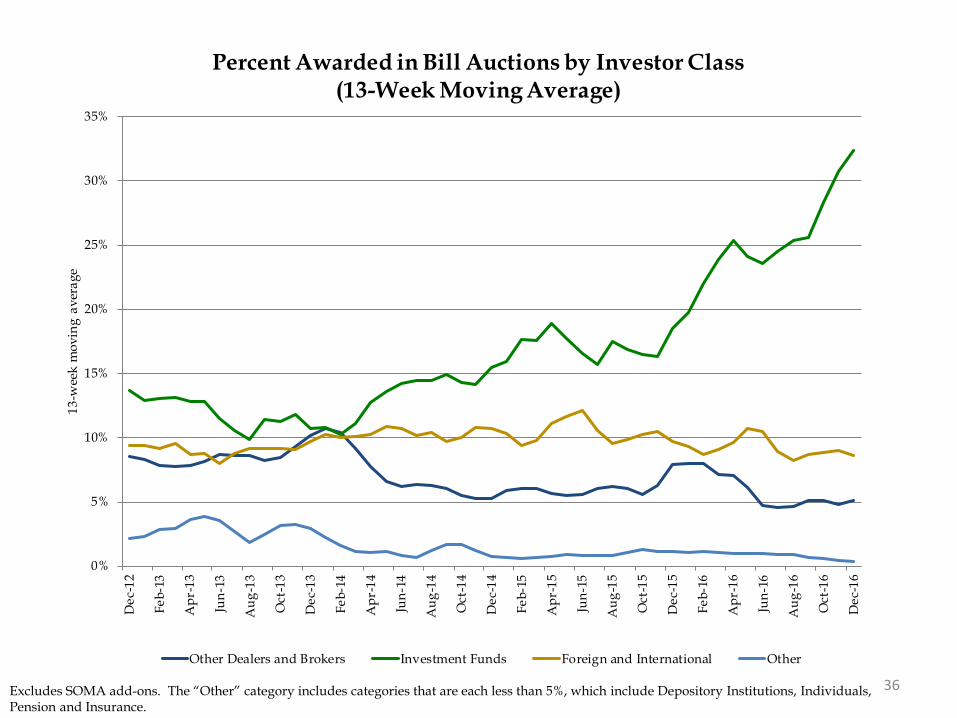
36 Excludes SOMA add-ons. The “Other” category includes categories that are each less than 5%, which include Depository Institutions, Individuals, Pension and Insurance.

0%

5%

10%

15%

20%

25%

30%

35%D

ec-1

2

Feb-

13

Apr

-13

Jun-

13

Aug

-13

Oct

-13

Dec

-13

Feb-

14

Apr

-14

Jun-

14

Aug

-14

Oct

-14

Dec

-14

Feb-

15

Apr

-15

Jun-

15

Aug

-15

Oct

-15

Dec

-15

Feb-

16

Apr

-16

Jun-

16

Aug

-16

Oct

-16

Dec

-16

13-w

eek

mov

ing

aver

age

Percent Awarded in Bill Auctions by Investor Class (13-Week Moving Average)

Other Dealers and Brokers Investment Funds Foreign and International Other


0%

5%

10%

15%

20%

25%

30%

35%

40%

45%

50%D

ec-1

2

Feb-

13

Apr

-13

Jun-

13

Aug

-13

Oct

-13

Dec

-13

Feb-

14

Apr

-14

Jun-

14

Aug

-14

Oct

-14

Dec

-14

Feb-

15

Apr

-15

Jun-

15

Aug

-15

Oct

-15

Dec

-15

Feb-

16

Apr

-16

Jun-

16

Aug

-16

Oct

-16

Dec

-16

6-m

onth

mov

ing

aver

age

Percent Awarded in 2-, 3-, and 5-Year Nominal Security Auctions by Investor Class (6-Month Moving Average)



0%

10%

20%

30%

40%

50%

60%D

ec-1

2

Feb-

13

Apr

-13

Jun-

13

Aug

-13

Oct

-13

Dec

-13

Feb-

14

Apr

-14

Jun-

14

Aug

-14

Oct

-14

Dec

-14

Feb-

15

Apr

-15

Jun-

15

Aug

-15

Oct

-15

Dec

-15

Feb-

16

Apr

-16

Jun-

16

Aug

-16

Oct

-16

Dec

-16

6-m

onth

mov

ing

aver

age

Percent Awarded in 7-, 10-, 30-Year Nominal Security Auctions by Investor Class (6-Month Moving Average)



0%

10%

20%

30%

40%

50%

60%

70%D

ec-1

2

Feb-

13

Apr

-13

Jun-

13

Aug

-13

Oct

-13

Dec

-13

Feb-

14

Apr

-14

Jun-

14

Aug

-14

Oct

-14

Dec

-14

Feb-

15

Apr

-15

Jun-

15

Aug

-15

Oct

-15

Dec

-15

Feb-

16

Apr

-16

Jun-

16

Aug

-16

Oct

-16

Dec

-16

6-m

onth

mov

ing

aver

age

Percent Awarded in TIPS Auctions by Investor Class(6-Month Moving Average)


40 Excludes SOMA add-ons.

20%

30%

40%

50%

60%

70%

80%D

ec-1

2

Feb-

13

Apr

-13

Jun-

13

Aug

-13

Oct

-13

Dec

-13

Feb-

14

Apr

-14

Jun-

14

Aug

-14

Oct

-14

Dec

-14

Feb-

15

Apr

-15

Jun-

15

Aug

-15

Oct

-15

Dec

-15

Feb-

16

Apr

-16

Jun-

16

Aug

-16

Oct

-16

Dec

-16

% o

f Tot

al C

ompe

titiv

e A

mou

nt A

war

ded

Primary Dealer Awards at Auction

4/13/26-Week (13-week moving average) 52-Week (6-month moving average)

2/3/5-Year (6-month moving average) 7/10/30-Year (6-month moving average)

TIPS (6-month moving average)

41 Excludes SOMA add-ons.

0%

5%

10%

15%

20%

25%

30%

Dec

-12

Feb-

13

Apr

-13

Jun-

13

Aug

-13

Oct

-13

Dec

-13

Feb-

14

Apr

-14

Jun-

14

Aug

-14

Oct

-14

Dec

-14

Feb-

15

Apr

-15

Jun-

15

Aug

-15

Oct

-15

Dec

-15

Feb-

16

Apr

-16

Jun-

16

Aug

-16

Oct

-16

Dec

-16

% o

f Tot

al C

ompe

titiv

e A

mou

nt A

war

ded

Direct Bidder Awards at Auction

4/13/26-Week (13-week moving average) 52-Week (6-month moving average)

2/3/5 (6-month moving average) 7/10/30 (6-month moving average)

TIPS (6-month-moving average)

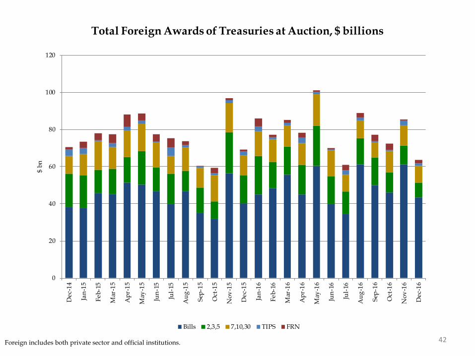
42 Foreign includes both private sector and official institutions.

0

20

40

60

80

100

120

Dec

-14

Jan-

15

Feb-

15

Mar

-15

Apr

-15

May

-15

Jun-

15

Jul-

15

Aug

-15

Sep-

15

Oct

-15

Nov

-15

Dec

-15

Jan-

16

Feb-

16

Mar

-16

Apr

-16

May

-16

Jun-

16

Jul-

16

Aug

-16

Sep-

16

Oct

-16

Nov

-16

Dec

-16

$ bn

Total Foreign Awards of Treasuries at Auction, $ billions

Bills 2,3,5 7,10,30 TIPS FRN

Appendix

43


0%

10%

20%

30%

40%

50%

60%

70%

80%

90%

100%

2017

2018

2019

2020

2021

2022

2023

2024

2025

2026

End of Fiscal Year

Projected Portfolio Composition by Issuance Type

Bills 2,3,5 7,10,30 TIPS (principal accreted to projection date) FRN

45

Recent and Projected Portfolio Composition by Issuance Type, Percent

This scenario does not represent any particular course of action that Treasury is expected to follow. Instead, it is intended to demonstrate the basic trajectory of average maturity absent changes to the mix of securities issued by Treasury.

End of Fiscal Year Bills 2-, 3-, 5-Year

Nominal Coupons

7-, 10-, 30-Year Nominal Coupons

Total Nominal Coupons

TIPS (principal accreted to projection date) FRN

2009 28.5 36.2 27.4 63.6 7.9 0.02010 21.1 40.1 31.8 71.9 7.0 0.02011 15.4 41.4 35.9 77.3 7.3 0.02012 15.0 38.4 39.0 77.4 7.5 0.02013 13.2 35.8 43.0 78.7 8.1 0.02014 11.5 33.0 46.0 79.0 8.5 1.02015 10.6 29.4 49.0 78.3 8.8 2.22016 12.1 27.0 49.6 76.6 8.9 2.42017 12.7 26.2 49.7 75.9 9.1 2.42018 12.2 26.0 50.0 76.0 9.4 2.32019 11.8 26.6 49.9 76.5 9.5 2.22020 11.4 27.0 50.1 77.1 9.5 2.12021 11.0 27.2 50.6 77.8 9.2 2.02022 10.5 27.4 51.2 78.6 9.0 1.92023 10.1 27.6 51.6 79.2 8.7 1.92024 9.7 27.5 52.4 79.9 8.6 1.82025 9.3 27.6 53.2 80.8 8.1 1.72026 9.0 27.7 53.9 81.6 7.8 1.7

46 *Weighted averages of Competitive Awards. **Approximated using prices at settlement and includes both Competitive and Non-Competitive Awards.

Issue Settle Date Stop Out Rate (%)*

Bid-to-Cover Ratio*

Competitive Awards ($bn)

% Primary Dealer* % Direct* %

Indirect*

Non-Competitive

Awards ($bn)

SOMA Add Ons

($bn)

10-Year Equivalent

($bn)*4-Week 10/6/2016 0.260 4.13 39.7 44.4 4.5 51.2 0.3 0.0 0.34-Week 10/13/2016 0.265 3.37 39.6 60.4 7.1 32.5 0.3 0.0 0.34-Week 10/20/2016 0.245 3.66 44.6 42.9 8.2 48.9 0.3 0.0 0.44-Week 10/27/2016 0.240 3.75 49.6 46.9 4.8 48.3 0.3 0.0 0.44-Week 11/3/2016 0.240 3.45 54.6 43.7 5.5 50.8 0.3 0.0 0.54-Week 11/10/2016 0.270 3.39 64.5 50.4 1.6 48.1 0.4 0.0 0.64-Week 11/17/2016 0.305 3.29 64.6 64.5 5.4 30.1 0.3 0.0 0.64-Week 11/25/2016 0.340 3.24 54.6 63.1 1.6 35.3 0.3 0.0 0.54-Week 12/1/2016 0.365 3.57 43.7 45.4 9.1 45.5 0.3 0.0 0.44-Week 12/8/2016 0.340 3.23 44.5 63.5 5.5 31.0 0.4 0.0 0.44-Week 12/15/2016 0.480 3.21 44.6 67.3 6.4 26.3 0.3 0.0 0.44-Week 12/22/2016 0.490 3.01 54.6 60.5 5.4 34.0 0.3 0.0 0.54-Week 12/29/2016 0.485 3.48 49.6 50.6 6.3 43.1 0.3 0.0 0.4

13-Week 10/6/2016 0.310 3.37 41.5 62.7 3.7 33.6 0.4 0.0 1.213-Week 10/13/2016 0.360 3.18 41.5 57.8 5.0 37.1 0.4 0.0 1.213-Week 10/20/2016 0.340 3.27 41.5 57.3 5.4 37.3 0.4 0.0 1.213-Week 10/27/2016 0.340 3.48 40.6 59.4 16.3 24.2 0.4 0.0 1.213-Week 11/3/2016 0.350 3.30 41.4 79.7 5.2 15.2 0.4 0.0 1.213-Week 11/10/2016 0.420 3.29 41.4 64.0 3.0 33.0 0.4 0.0 1.213-Week 11/17/2016 0.515 3.13 41.4 49.2 5.5 45.2 0.4 0.0 1.213-Week 11/25/2016 0.480 3.53 38.4 60.0 3.9 36.2 0.4 0.0 1.113-Week 12/1/2016 0.490 3.84 34.7 59.7 5.0 35.3 0.3 0.0 1.013-Week 12/8/2016 0.490 3.64 33.5 52.7 9.3 38.0 0.4 0.0 0.913-Week 12/15/2016 0.530 3.71 33.4 53.3 6.6 40.1 0.4 0.0 1.013-Week 12/22/2016 0.515 3.19 33.3 57.1 7.6 35.3 0.5 0.0 1.013-Week 12/29/2016 0.555 3.44 32.6 55.5 1.6 42.9 0.4 0.0 1.026-Week 10/6/2016 0.490 3.58 35.2 47.6 2.3 50.2 0.4 0.0 2.026-Week 10/13/2016 0.495 3.50 35.2 40.0 2.0 58.0 0.3 0.0 2.026-Week 10/20/2016 0.470 3.30 35.4 44.6 2.7 52.7 0.3 0.0 2.026-Week 10/27/2016 0.475 3.50 34.7 50.8 5.0 44.2 0.3 0.0 2.026-Week 11/3/2016 0.500 3.48 35.2 54.6 1.9 43.4 0.4 0.0 2.026-Week 11/10/2016 0.535 3.41 35.5 47.7 1.4 50.9 0.3 0.0 2.026-Week 11/17/2016 0.625 3.13 35.5 41.1 2.0 56.9 0.3 0.0 2.026-Week 11/25/2016 0.605 3.84 32.4 44.3 0.9 54.8 0.3 0.0 1.826-Week 12/1/2016 0.610 4.27 28.8 33.2 2.3 64.6 0.3 0.0 1.726-Week 12/8/2016 0.615 3.72 27.6 53.6 3.2 43.3 0.3 0.0 1.626-Week 12/15/2016 0.645 3.63 27.5 34.9 2.8 62.3 0.4 0.0 1.626-Week 12/22/2016 0.645 3.35 27.5 56.0 2.5 41.4 0.4 0.0 1.626-Week 12/29/2016 0.660 3.83 26.7 31.8 1.3 66.8 0.3 0.0 1.652-Week 10/13/2016 0.680 3.46 19.8 53.5 2.2 44.3 0.2 0.0 2.252-Week 11/10/2016 0.695 3.35 19.8 63.3 1.5 35.2 0.2 0.0 2.252-Week 12/8/2016 0.830 3.58 19.8 53.0 5.1 41.9 0.2 0.0 2.2

Bills

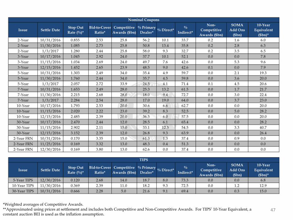
47 *Weighted averages of Competitive Awards. **Approximated using prices at settlement and includes both Competitive and Non-Competitive Awards. For TIPS’ 10-Year Equivalent, a constant auction BEI is used as the inflation assumption.


Bid-to-Cover Ratio*



Indirect*

Non-Competitive

Awards ($bn)

SOMA Add Ons

($bn)

10-Year Equivalent

($bn)*2-Year 10/31/2016 0.855 2.53 25.8 56.2 10.1 33.7 0.2 1.6 6.02-Year 11/30/2016 1.085 2.73 25.8 50.8 13.4 35.8 0.2 2.8 6.32-Year 1/3/2017 1.280 2.44 25.8 58.0 9.3 32.7 0.2 3.5 6.53-Year 10/17/2016 1.045 2.92 24.0 37.7 10.1 52.1 0.0 0.0 7.83-Year 11/15/2016 1.034 2.69 24.0 49.7 7.6 42.6 0.0 5.3 9.63-Year 12/15/2016 1.452 2.65 23.9 48.5 9.0 42.6 0.1 0.0 7.95-Year 10/31/2016 1.303 2.49 34.0 35.4 4.9 59.7 0.0 2.1 19.35-Year 11/30/2016 1.760 2.44 34.0 35.7 4.5 59.8 0.0 3.6 20.05-Year 1/3/2017 2.057 2.72 33.9 24.5 4.1 71.4 0.1 4.5 20.67-Year 10/31/2016 1.653 2.49 28.0 25.3 13.2 61.5 0.0 1.7 21.77-Year 11/30/2016 2.215 2.68 28.0 18.0 9.4 72.7 0.0 3.0 22.47-Year 1/3/2017 2.284 2.54 28.0 17.0 19.0 64.0 0.0 3.7 23.0

10-Year 10/17/2016 1.793 2.53 20.0 30.6 6.6 62.7 0.0 0.0 20.010-Year 11/15/2016 2.020 2.22 23.0 39.2 8.3 52.5 0.0 5.0 28.210-Year 12/15/2016 2.485 2.39 20.0 36.5 6.0 57.5 0.0 0.0 20.030-Year 10/17/2016 2.470 2.44 12.0 28.5 6.1 65.4 0.0 0.0 28.230-Year 11/15/2016 2.902 2.11 15.0 33.1 12.5 54.5 0.0 3.3 40.730-Year 12/15/2016 3.152 2.39 12.0 26.8 9.3 63.9 0.0 0.0 26.4

2-Year FRN 10/31/2016 0.170 3.35 15.0 61.3 1.3 37.4 0.0 0.9 0.02-Year FRN 11/25/2016 0.169 3.32 13.0 48.3 0.4 51.3 0.0 0.0 0.02-Year FRN 12/30/2016 0.169 3.80 13.0 62.6 0.0 37.4 0.0 0.0 0.0


Bid-to-Cover Ratio*



Indirect*

Non-Competitive

Awards ($bn)

SOMA Add Ons

($bn)

10-Year Equivalent

($bn)*5-Year TIPS 12/30/2016 0.120 2.68 14.0 18.7 8.0 73.3 0.0 0.0 6.8

10-Year TIPS 11/30/2016 0.369 2.39 11.0 18.2 9.3 72.5 0.0 1.2 12.930-Year TIPS 10/31/2016 0.666 2.28 5.0 21.6 9.1 69.4 0.0 0.3 15.0

Nominal Coupons

TIPS

January 2017

T B A C C H A R G E Q U E S T I O N : O P T I M I Z A T I O N M O D E L S F O R T R E A S U R Y D E B T

S T

R I C

T L

Y

P R

I V

A T

E

A N

D

C O

N F

I D

E N

T I A

L

T B

A C

C

H A

R G

E

Q U

E S

T I O

N :

O P

T I M

I Z

A T

I O

N

M O

D E

L S

F

O R

T

R E

A S

U R

Y

D E

B T

January 31, 2017

Charge Question

The primary objective of Treasury’s debt management strategy is to finance the government’s borrowing needs at the

lowest risk-adjusted cost over time. To accomplish this, Treasury strives to issue debt in a regular and predictable

pattern, but that approach leaves open a wide range of potential outcomes for the maturity structure of the debt. The

interest expense associated with any issuance strategy will depend on a variety of factors that are not under the

control of the debt manager, including the behavior of interest rates, the business cycle, and the federal government’s

fiscal policy. A number of countries including the United States have developed quantitative models that can assist in

the evaluation of alternative financing strategies in the face of inherent uncertainty about the future. Treasury

requests the Committee’s input on the appropriate considerations for and use of these types of models, consistent

with their ability to calculate interest expense associated with alternative issuance scenarios and to help debt

managers better understand the implications of various financing choices.

1

Agenda

Page

T B

A C

C

H A

R G

E

Q U

E S

T I O

N :

O P

T I M

I Z

A T

I O

N

M O

D E

L S

F

O R

T

R E

A S

U R

Y

D E

B T

2

Historical Cost of Alternative Issuance Strategies in the US

2

Debt Management Models Developed by Other Countries 8

A Debt Optimization Framework for US Treasuries 16

Appendix 23

H I S

T O

R I C

A L

C

O S

T

O F

A

L T

E R

N A

T I V

E

I S

S U

A N

C E

S

T R

A T

E G

I E

S I N

T

H E

U

S

Historical US Treasury Rates By Quarter

As background to our discussion on key components of a US debt optimization model, we consider what issuance

strategies have had the lowest cost historically in the US

0

2

4

6

8

10

12

14

16

18

July-61 July-65 July-69 July-73 July-77 July-81 July-85 July-89 July-93 July-97 July-01 July-05 July-09 July-13

His

tori

ca

l U

S T

rea

sury

In

tere

st R

ate

Le

ve

ls (

%)

3 Month 2 Year 5 Year 10 Year 30 Year

3

H I S

T O

R I C

A L

C

O S

T

O F

A

L T

E R

N A

T I V

E

I S

S U

A N

C E

S

T R

A T

E G

I E

S I N

T

H E

U

S

(10)

(5)

0

5

10

15

20


His

tori

ca

l R

ate

s a

nd

Ro

llin

g A

ve

rag

e R

ate

s (%

)

2 Year Rate Level Average Rate Rolling For Next 2 Years Realized Term Premium

Historical Premium Of Issuing Term Debt Compared To Rolling Short Debt

2 Year Realized Term Premium = Spot 2 Year Rate - Average 3M Rate Rolling For Next 2 Years

4

H I S

T O

R I C

A L

C

O S

T

O F

A

L T

E R

N A

T I V

E

I S

S U

A N

C E

S

T R

A T

E G

I E

S I N

T

H E

U

S

(10)

(5)

0

5

10

15

20


His

tori

ca

l R

ate

s a

nd

Ro

llin

g A

ve

rag

e R

ate

s (%

)


Historical Premium of Issuing Term Debt Compared to Rolling Short Debt

5 Year Realized Term Premium = Spot 5 Year Rate – Average 3M Rate Rolling For Next 5 Years

5

H I S

T O

R I C

A L

C

O S

T

O F

A

L T

E R

N A

T I V

E

I S

S U

A N

C E

S

T R

A T

E G

I E

S I N

T

H E

U

S

(10)

(5)

0

5

10

15

20


His

tori

ca

l R

ate

s a

nd

Ro

llin

g A

ve

rag

e R

ate

s (%

)


Historical Premium of Rolling Short Debt vs Issuing Term Debt

10 Year Realized Term Premium = Spot 10 Year Rate - Average 3M Rate Rolling For Next 10 Years

6

H I S

T O

R I C

A L

C

O S

T

O F

A

L T

E R

N A

T I V

E

I S

S U

A N

C E

S

T R

A T

E G

I E

S I N

T

H E

U

S

US Treasury Interest Expense Over Historical 5 Year Intervals

Rates

Generally

Increasing

Rates

Generally

Decreasing

The below table shows interest expense and average interest rate paid during 5 year intervals over the last 50

years

Each strategy involves the issuer maintaining a fixed amount of outstanding debt by issuing debt of a maturity M

where 1/M of outstanding debt is scheduled to mature each period; in this case, interest expense will be a

simple rolling average of historical interest rates

While interest rates have oscillated, rates generally increased prior to 1981 and decreased after 1981

Longer-term debt strategies perform better as rates increase; shorter-term strategies perform better as rates

decrease

In this dataset, the benefit of longer-term issuance in rising rate environments is small relative to its disadvantage

in declining rate environments

3 Month 2 Year 5 Year 10 Year 3 Month 2 Year 5 Year 10 Year

1967-71 $28.0 $29.0 $25.7 $23.7 5.60 5.79 5.14 4.73

1972-76 $30.7 $33.5 $33.4 $29.8 6.13 6.69 6.68 5.96

1977-81 $50.5 $43.7 $40.0 $37.1 10.10 8.74 8.01 7.43

1982-86 $44.4 $57.0 $57.9 $49.4 8.87 11.41 11.58 9.88

1987-91 $35.2 $39.3 $45.2 $52.6 7.04 7.86 9.04 10.52

1992-96 $21.6 $27.7 $35.3 $42.5 4.32 5.53 7.05 8.51

1997-01 $25.1 $28.2 $30.0 $34.9 5.03 5.64 6.00 6.98

2002-06 $12.5 $15.0 $22.3 $28.7 2.50 2.99 4.46 5.73

2007-11 $7.7 $12.5 $18.0 $23.6 1.55 2.50 3.60 4.73

2012-16 $1.3 $2.2 $8.0 $17.6 0.26 0.44 1.60 3.53

5 Year Interest Expense Per $100 Issued Average % Rate Paid Over 5 Year Intervals

Interest expense and average rate paid

7

Agenda

Page

T B

A C

C

H A

R G

E

Q U

E S

T I O

N :

O P

T I M

I Z

A T

I O

N

M O

D E

L S

F

O R

T

R E

A S

U R

Y

D E

B T

8

Debt Management Models Developed by Other Countries

8

Historical Cost of Alternative Issuance Strategies in the US 2


Appendix 23

D E

B T

M

A N

A G

E M

E N

T

M O

D E

L S

D

E V

E L

O P

E D

B

Y

O T

H E

R

C O

U N

T R

I E

S

Government Debt Optimization Models

Many sovereign debt managers utilize stochastic simulation/optimization models to help inform their decisions about

debt issuance and the optimal maturity structure of government debt.

The Debt Management Office of Canada, UK, Sweden, Brazil, and Turkey have all published detailed working

papers highlighting the key components of their models. Other countries (e.g., Denmark, Austria, Portugal and

Belgium) have indicated that they utilize stochastic simulations of alternative debt management strategies.*

The models are generally used to help quantify the tradeoffs debt managers face between the expected cost of debt

issuance over time and the variability of these costs across different scenarios.

In a survey of 71 public debt managers conducted by the US Treasury and World Bank at the 2012 Sovereign Debt

Managers forum, more than half of managers said their debt strategy is supported by stochastic simulation models

that quantify risk/cost tradeoffs. While the survey indicated that 100% of HIC’s (high income countries) had a debt

management strategy that was supported by quantitative analysis, only about one-third (37%) had published details

of the model underlying their strategy.

* See for example Bolder and Deeley, “The Canadian Debt-Strategy Model: An Overview of the Principal Elements”, 2011; Pick and Anthony, “A Simulation model for the analysis of the UK’s sovereign debt

strategy”, 2006; “The SNDO’s Simulation Model for Government Debt Analysis”, 2002 and Advances in Risk Management of Public Debt,, OECD 2005.

27%29%

31%

13%

0%

5%

10%

15%

20%

25%

30%

35%

Yes, deterministic andstochastic

Yes stochastic models Yes, deterministic models No

2012 Sovereign Debt Managers forum survey results on whether the manager has a formal debt management

strategy based on quantitative analysis

9

D E

B T

M

A N

A G

E M

E N

T

M O

D E

L S

D

E V

E L

O P

E D

B

Y

O T

H E

R

C O

U N

T R

I E

S

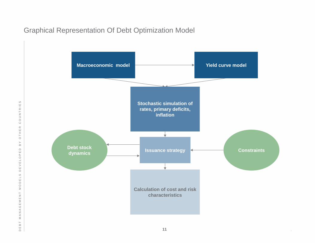
Key Components Of Debt Simulation/Optimization Models

In broad terms, the models used by debt managers (including the US Treasury) are quite similar and generally

involve the following four key components:

A simple macroeconomic model that can be used to generate stochastic simulations of different economic and

interest rate environments.

A term structure model for relating the yield curve to short rates.

An objective function of the debt manager that typically involves minimizing expected issuance costs through

time subject to constraints on risk and other variables.

An optimization module that identifies low cost strategies given alternative risk and issuance constraints.

The models are primarily used to quantify tradeoffs between cost and risk (i.e., an efficient frontier) rather than

identifying a single optimal strategy.

10

D E

B T

M

A N

A G

E M

E N

T

M O

D E

L S

D

E V

E L

O P

E D

B

Y

O T

H E

R

C O

U N

T R

I E

S

Graphical Representation Of Debt Optimization Model

Constraints Debt stock

dynamics

Macroeconomic model Yield curve model

Stochastic simulation of

rates, primary deficits,

inflation

Issuance strategy

Calculation of cost and risk

characteristics

11

0.0

0.5

1.0

1.5

2.0

2.5

3.0

3.5

4.0

2014 2016 2018 2020 2022 2024 2026

Estimated Monetary Policy Rule Implied forward Actual

D E

B T

M

A N

A G

E M

E N

T

M O

D E

L S

D

E V

E L

O P

E D

B

Y

O T

H E

R

C O

U N

T R

I E

S

Overview Of Macroeconomic And Yield Curve Models

Macro models used by debt managers typically involve separate equations for the output gap, inflation, short term

policy rates, and the primary deficit.

A variety of yield curve models are used by debt managers to generate stochastic paths for interest rates as a

function of the macroeconomic environment.

One shortcoming of all of the macro models used in published papers on debt optimization is the lack of any

clear link between short term rates derived from the model and forward rates implied from the yield curve.

This disconnect is potentially important in the U.S. where most macroeconomic models currently produce a

much steeper path for the funds rate than what is implied by market forward rates and estimates of the term

premium (see Chart).

Testing the robustness of optimization results to alternative yield curve assumptions should be a key component

of debt optimization.

Projected Fed funds rate derived from a simple macroeconomic model of the US economy (%)

12

D E

B T

M

A N

A G

E M

E N

T

M O

D E

L S

D

E V

E L

O P

E D

B

Y

O T

H E

R

C O

U N

T R

I E

S

Objective Function And Risk Constraints

Most of the simulation/optimization models in use include an objective function that minimizes expected costs of

new debt issuance over a long term horizon.

Expectations are taken over multiple paths for interest rates, deficits, and inflation.

Choice variables include allocation across different points on the yield curve usually constructed to be constant

weights through time.

Objective function

Constraints

Risk constraints relate to limits on variability of either debt expense or fiscal balance.

Constraints based on fiscal balance incorporate correlation between rates and primary deficits and are better

aligned with academic literature that highlight social welfare benefits from tax smoothing.*

Risk measures used are either a standard volatility measure (e.g. standard deviation of debt expense or budget)

or a VAR type limit (e.g. 95% confidence interval).

Risk measures could also be incorporated directly into the objective function in a way that is mathematically

equivalent to having them as a constraint.

Other constraints typically considered reflect a desire for regular and predictable issuance and include:

Limiting the change in issuance amount for each tenor from period-to-period

Limiting the overall WAM

Maintaining a specified amount of issuance at various points on the curve (in order to support market liquidity

and/or regulatory objectives).

An issuance penalty function that increases cost with issue size.

* See for example Barro, 1974. “Are Government Bonds New Wealth?” Journal of Political Economy 83, no.6 (November-December):1095-117

13

D E

B T

M

A N

A G

E M

E N

T

M O

D E

L S

D

E V

E L

O P

E D

B

Y

O T

H E

R

C O

U N

T R

I E

S

Some Differences In Models Used By Sovereign Debt Managers In Other

Countries

Many differences exist in the exact specification of costs and risks in the published models.

Debt costs can be measured in absolute dollars, as a percent of outstanding debt, or as a percent of GDP; costs

can be discounted or undiscounted.

Risk can be calculated at a single point in time or averaged over all time periods (the Canadian model is one of

the few that provide actual simulation results showing how the cost-risk tradeoff is impacted by alternative risk

specifications).

Countries that must take credit risk into consideration (i.e., countries with elevated public indebtedness or emerging

market economies) tend to view debt management as part of an integrated asset/liability framework.

There are variety of different approaches used to establish the initial conditions for the simulation. For example,

Sweden starts with a portfolio that matches the specified strategy while the UK uses the actual portfolio as a

jumping off point but sets the initial values for macroeconomic variables and the yield curve on the basis of long run

historical averages.

The issuance of foreign currency debt can create significant modelling complications.

Differences in yield curves and yield curve models can have a significant effect on results

In the UK model, the optimal cost–risk tradeoff is generally achieved by skewing issuance toward long maturity

Gilts. This seems attributable to an assumption that the yield curve is downward sloping at the long end of the

curve.

In the UK model, It can take 20 years or more to achieve a steady state cost outcome. This likely reflects the

inclusion of a meaningful amount of 30-year and 50-year maturities (for both nominal and inflation-linked gilts) in

the issuance mix.

14

D E

B T

M

A N

A G

E M

E N

T

M O

D E

L S

D

E V

E L

O P

E D

B

Y

O T

H E

R

C O

U N

T R

I E

S

Key Insights On Issuance From The Published Models

Intermediate issuance:

Optimization models often find the most attractive risk reduction per unit of cost by extending from bills to

intermediates (e.g. 5-year); the risk reduction per unit of cost tends to be lower when extending further out the

curve.

Optimal intermediate issuance levels appear more stable in response to changes in model parameters/risk

constraints than front-end and long-end issuance.

Bill issuance and liquidity demand:

Constraining the optimization to have higher levels of bill issuance (e.g., in order to meet market needs for

liquidity) appears to have the largest impact on reducing 10- and 30-year issuance in debt optimization with

smaller effects on intermediates.

Constraints on debt cost volatility vs. budget volatility:

Setting risk constraints on the volatility of the fiscal balance rather than debt cost volatility generally results in

higher levels of short term debt in the optimization; this reflects the negative correlation between interest rates

and primary deficits.

Inflation linked bonds:

Inflation linked bonds provide a diversification benefit and reduce volatility especially when the binding

constraints are on budgetary volatility; at low target levels of volatility, the optimal issuance strategy can include

substantial amounts of inflation linked bonds.

Other constraints:

When issuance is constrained by a target WAM, 30-year debt has a larger weight; this reflects the fact that the

marginal impact of 30-year debt on WAM is larger per unit of cost relative to 5-year and 10-year bonds.

The inclusion of Issuance penalties that include additional costs from issuing in large size reduces the incidence

of corner solutions with debt more evenly allocated across the curve.

15

Agenda

Page

T B

A C

C

H A

R G

E

Q U

E S

T I O

N :

O P

T I M

I Z

A T

I O

N

M O

D E

L S

F

O R

T

R E

A S

U R

Y

D E

B T

16

A Debt Optimization Framework for US Treasuries

16



Appendix 23

A

D E

B T

O

P T

I M

I Z

A T

I O

N

F R

A M

E W

O R

K

F O

R

U S

T

R E

A S

U R

I E

S

Motivation For Constructing A U.S. Debt Model

A model allows a richer framework for considering debt management decisions than the historical exercise shown

earlier

Simulate the range of outcomes that could take place going forward under various assumptions about the

economy and interest rates

Measure some of the trade-offs involved in debt management decisions

Explore the sensitivity of those trade-offs to different assumptions about the behavior of the economy and rates

TBAC members have been working on several different models that could be applied to the U.S. Treasury market

All models are a work in progress at this point

This presentation will show some preliminary results from one of those models

Those results provides an initial look at whether we see some of the same patterns that were described above

for the models from other countries

This effort should complement the work by the Office of Debt Management

ODM’s quantitative strategies group has done extensive modeling of debt dynamics (see appendix for more

detail)

Highly detailed models for tracking and analyzing debt characteristics, and able to do simulations to assess

various debt management issues

Likely to be synergy between the various modeling efforts

17

A

D E

B T

O

P T

I M

I Z

A T

I O

N

F R

A M

E W

O R

K

F O

R

U S

T

R E

A S

U R

I E

S

Structure Of The Model: Macro Equations

Structure of the model involves equations for the following variables:

Unemployment rate (IS curve, expressed in terms of gap from full employment)

Inflation (Phillips curve)

Short -term interest rates (monetary policy rule)

Primary deficit (equation relating to business cycle)

This structure describes macroeconomic dynamics in order to capture their effects on the evolution of Treasury borrowing

needs and its funding rates

Simulations of the model can be used to measure the uncertainty about these variables

Core PCE inflation

(QoQ SAAR)

Fed funds rate

(%)

Primary budget balance

(% of GDP)

Unemployment rate

(%)

2.0

2.5

3.0

3.5

4.0

4.5

5.0

5.5

6.0

6.5

20

17

20

19

20

21

20

23

20

25

20

27

Mean

15th/85th percentile

0

1

2

3

4

5

20

17

20

19

20

21

20

23

20

25

20

27

Mean


-5

-4

-3

-2

-1

0

1

2

3

20

17

20

19

20

21

20

23

20

25

20

27

Mean


0

1

2

3

4

5

6

7

8

20

17

20

19

20

21

20

23

20

25

20

27

Mean


18

A

D E

B T

O

P T

I M

I Z

A T

I O

N

F R

A M

E W

O R

K

F O

R

U S

T

R E

A S

U R

I E

S

Structure Of The Model: Treasury Yield Equations

Model explicitly focuses on the evolution of term premiums

Useful given the key importance of the term premium in debt management decisions

The current version relies on a measure of term premiums from outside the model

Using the term premium measures from Adrian, Crump, and Moench (2013)*

Introduces some inconsistency with the structure of the macro equations that we assume gradually dissipates

Macro variables in the model explain some, but not all, of the variation in term premiums

Rest of movements are assumed to be persistent but eventually mean-reverting

History of ACM Term Premium Measures

(pp)

Distribution of Term Premium Measures in 10 Years

(pp)

-1.0

-0.5

0.0

0.5

1.0

1.5

2.0

2.5

3.0

3.5

4.0

1995 2000 2005 2010 2015

2-year 10-year

0.0

0.1

0.1

0.2

0.2

0.3

0.3

0.4

-1.6

25

-1.3

75

-1.1

25

-0.8

75

-0.6

25

-0.3

75

-0.1

25

0.1

25

0.3

75

0.6

25

0.8

75

1.1

25

1.3

75

1.6

25

1.8

75

2.1

25

2.3

75

2.6

25

2.8

75

Fre

qu

en

cy

2-year 10-year

19

* Adrian, Tobias, Crump, Richard, Moench, Emanuel, 2013. “Pricing the term structure with linear regression”, Journal of Financial Economics

A

D E

B T

O

P T

I M

I Z

A T

I O

N

F R

A M

E W

O R

K

F O

R

U S

T

R E

A S

U R

I E

S

Structure Of The Model: Other Components

Structure captures how yield curve and deficits evolve given economic and other shocks

Determines the correlation of borrowing costs with deficits

Can run simulations for the next 10 years and beyond

Debt stock dynamics

Track outstanding debt in terms of its maturity distribution and costs

Primary deficit and debt cost determine total budget deficit

Total deficit and maturing debt determine gross issuance needs

Issuance assumptions

Need to make assumptions about how new issuance will be allocated across maturities

Here consider hypothetical issuance strategies where all debt issued at a single maturity point

These strategies are not realistic, but are simply intended to demonstrate trade-offs in the model

In running these simulations, we are ignoring constraints on issue sizes or any pressure on yields from supply

Relevant statistics for debt management

We compute a variety of statistics for average debt cost and the variability of the budget under these

assumptions

These statistics are computed for the simulated values at the end of a 10-year horizon

20

A

D E

B T

O

P T

I M

I Z

A T

I O

N

F R

A M

E W

O R

K

F O

R

U S

T

R E

A S

U R

I E

S

10-years ahead Bills only 2y only 5y only 10y only 30y only

Average issuance rate 2.93 2.99 3.27 3.72 4.37

Average debt service / GDP 2.60 2.63 2.92 3.22 4.00

Standard deviation debt service / GDP 1.74 1.35 0.53 0.51 0.61

Standard deviation issuance rate 2.22 1.97 1.09 0.69 0.46

Standard deviation primary deficit / GDP 2.24 2.24 2.24 2.24 2.24

Correlation of issuance rate w/ primary deficit -0.41 -0.55 -0.54 -0.15 -0.13

Standard deviation total deficit / GDP 2.37 2.48 2.50 2.52 2.59

Average WAM 1.4 2.1 3.3 5.1 23.6

Standard deviation WAM 0.1 0.1 0.1 0.3 0.4

Average WAC 2.97 3.00 3.24 3.49 4.15

Standard deviation WAC 2.04 1.61 0.61 0.26 0.17

Average debt / GDP 85 85 86 87 92

Standard deviation debt / GDP 11 12 15 16 16

*Based on simulations of 10,000 paths per issuance strategy.

Issuance strategy

Macro Debt Model Simulations*

Relevant Statistics Under Concentrated Issuance Strategies

21

A

D E

B T

O

P T

I M

I Z

A T

I O

N

F R

A M

E W

O R

K

F O

R

U S

T

R E

A S

U R

I E

S

Preliminary Observations From The Results

The average cost of the debt is upward sloping in maturity of issuance

This pattern reflects the fact that the term premium in the model reverts to an average level that is upward

sloping in maturity

A key issue is whether to assume this type of reversion towards historical averages

If the term premium instead stays closer to its current levels, long-term debt would be more attractive than

suggested in the above results.

The variation in debt cost falls notably as the maturity extends to intermediate horizons

This finding is similar to the result from other models—that a considerable reduction in the variability of debt cost

is realized by extending from bills out to around the 5-year sector

The variability stabilizes and turns slightly higher at long maturities because of the variability of the term premium

and the larger amount of debt that occurs when issuing at higher cost

The correlation of rates and the economy makes issuing shorter-term debt more attractive

The standard deviation of the budget could be considered a more relevant measure for debt management than

the standard deviation of the debt cost

The correlation of interest rates with the economy favors issuing shorter-term debt relative to longer-term debt

under this metric

This pattern arises because issuing shorter term debt makes interest expense pro-cyclical, offsetting the counter-

cyclical nature of the primary deficit

22

Agenda

Page

T B

A C

C

H A

R G

E

Q U

E S

T I O

N :

O P

T I M

I Z

A T

I O

N

M O

D E

L S

F

O R

T

R E

A S

U R

Y

D E

B T

23

Appendix

23




A P

P E

N D

I X

Debt Model Currently Used By US Treasury Office Of Debt Management

QSG within the Office of Debt Management (ODM) has developed a number of quantitative models that are used in

policy and market analyses

ODM debt issuance models include the following characteristics:

Forward portfolio simulation for either 1yr for short term and 10yr for long term

– Simulations are at the CUSIP-level and provides daily cash flows

Rates, deficits, CPI, SOMA assumptions (POMO purchases, sells, and reinvestment policy) are inputs which

define a scenario

– Daily fiscal flows projections provided from the Office of Fiscal Projections are used for short term model

– Primary deficit, net interest, and other transactions affecting the borrowing from the public are provided by

OMB and CBO’s budget are used as inputs for the long term model.

Issue sizes constraints: lower/upper bounds, bounds on size changes, number of CMBs, issue ratios, etc.

– Supply feedback effect on rates implicitly controlled by maximum size changes

Cash balance constraints: lower/upper bounds, hard targets on specific date(s), generally sufficient to cover

one week of outflows, etc.

Optimize future issue sizes to minimize the present value of future debt-service costs

– Linear programming problem

– (rates, CPI, deficits, SOMA, constraints …) Optimal-cost issuance/metrics

Fix market assumptions, vary constraints: see tradeoffs involved in changing policy (as embodied by

constraints)

Fix constraints, vary market assumptions: see risk attached to a fixed policy window

Rate, CPI, deficit inputs may be stochastic (Monte Carlo simulation)

– ODM has developed an internal joint nominal and real term structure model with shadow rate.

– ODM has also implemented ACM term structure model for internal use.

– Able to test Fed rate hike/hold scenarios as well as highly volatile rate environment.

24

treasury presentation to tbac - united states … of treasury’s february 2017 quarterly refunding...

Documents