This document has been made available through Treasures at UT Dallas, a service of the Eugene McDermott Library. Please contact libwebhelp@utdallas.edu for additional information.

Treasures at UT Dallas

Eric Jonsson School of Engineering and Computer Science

6-2009

Finding a Simple Path with Multiple Must-include Nodes Hars Vardham, et al.

Follow this and additional works at: http:// http://libtreasures.utdallas.edu/xmlui/handle/10735.1/2637

Finding a Simple Pathwith Multiple Must-include Nodes

Technical Report UTD/EE/2/2009

June 2009

Hars Vardhan∗, Shreejith Billenahalli∗, Wanjun Huang∗, Miguel Razo∗, Arularasi Sivasankaran∗,Limin Tang∗, Paolo Monti†, Marco Tacca∗, and Andrea Fumagalli∗

∗Open Networking Advance Research (OpNeAR) LabErik Jonsson School of Engineering and Computer ScienceThe University of Texas at Dallas, Richardson, TX, USA

andreaf@utdallas.edu†Next Generation Optical Network (NeGONet) Group

School of Information and Communication Technology, ICT-FMIThe Royal Institute of Technology, Kista, Sweden

pmonti@kth.se

Abstract

This document presents an algorithm to find a simple path in the given network with multiple must-includenodes. The problem of finding a simple path with only one must-include node can be solved in polynomial timeusing lower bound max-flow approach. However, including multiple nodes in the path has been shown to be aNP-Complete. This problem may arise in network areas such as forcing the route to go through particular nodes,which have wavelength converter (optical), have monitoring provision (telecom), have gateway functions (in OSPF)or are base stations (in MANET). Also, network standards allow loose definition of routing by requiring one ormore nodes to be in the routing of Link State Packet. In this document, a heuristic algorithm is described to find asimple path between a pair of terminals, which has constraint to pass through a certain set of other nodes.

The algorithm is comprised into two main steps: (1) considering a pair of nodes in sequence from source todestination as a segment and then computing candidate paths between each segment, and (2) combining paths, onefrom each segment, in order to make simple path from source to destination. The max-flow approach is used to findcandidate paths, a which provides maximum number of edge disjoint paths for individual segments. The secondstep of the algorithm uses backtracking algorithm for combining paths. The time complexity of the first step of thealgorithm is O(k|V ||E|2), where k is the number of must-include nodes. The time complexity of step (2) dependsupon total number of candidate paths which are not touching any one of the candidates of other segments. So, theworse case time complexity of step (2) is O(λk), where λ is the maximum nodal degree of the network. However, weshow that step (2) has minimal effect on the algorithm and it does not grow exponentially with k in this application.Later, we also show that initial re-ordering of the given sequence of must-include nodes can improve the result. Theexperimental results show that the algorithm is successful in computing near optimal path in reasonable time.keywords: constrained path computation, graph theory, heuristic algorithm, max flow, network route.

I. INTRODUCTION

Network standards [1] [2] [3] allow loose definition of routing by requiring one or more nodes to be in the route

of Link State Packet. This problem may arise in various networking areas such as optical networks, OSPF (Open

Shortest Path First) protocol, telecommunication networks, and MANET (Mobile ad-hoc networks). For example,

the optical network routing may require the route to include some specific nodes, which are wavelength converter or

amplifier/regenerator enabled. OSPF network may have some of the nodes to act as gateways across the subnetwork,

which must be included in the path when source and destination are multiple subnet apart. In telecommunication

network, routing of the traffic may be forced to go through specific nodes that have traffic monitoring capability.

MANET often require routes through some designated nodes, which are directly connected to a base station.

The problem of including only one node in the computation of a simple path is polynomial time solvable using,

for example lower bound max-flow [4], as briefly described next. The lower bound max-flow algorithm computes a

flow, which must include all the edges that have a positive (> 0) lower bound value. If only one edge has a positive

lower bound, the flow computed by the algorithm can be used to build a simple path, which includes such edge.

The “edge” instance of the problem can be transformed into its “node” equivalent by first splitting the include-node

into two half-nodes, i.e., n1 and n2. All incoming edges to the original node converge to n1. All outgoing edges of

the original node emerge from n2. A directed edge el from n1 to n2 is added with a positive lower bound value.

All other (original) edges of the network have zero lower bound. Now, applying the lower bound max-flow [5]

algorithm to this flow network, a feasible flow from source to destination can be found such that el is included in

at least one of the (flow) augmenting paths. Then on merging n1 and n2 the simple path can be traced. The lower

bound max-flow technique cannot be successfully applied to 2 or more include nodes, as there is not a guarantee

that the same augmenting path in the flow algorithm contains all of them at once. Hence, it is not possible to trace

out a simple path with all of the must-include nodes.

The shortest path with multiple must-include nodes can be seen as a more general case of the well known

traveling salesman path (TSP) problem, which is NP-complete1. Instead of traveling all nodes as in the original

TSP, this problem requires to travel only a subset of the nodes from source to destination. This problem can be

solved by brute-force method of complete enumeration of all the possible paths and then choosing the best path

which contains all must-include nodes. Akin to the TSP problem, the number of enumerations in the problem is

exceedingly large [8]. Given a network of n(= |V |) nodes, the number of possible such tours is exponential, or

more precisely O(n!). On the other hand, if a path is given from source to destination then it can be verified in

polynomial time whether it includes all the nodes of I . Given a path P , presence of any loop in P can be checked

1The TSP problem and its variations have been addressed by a number of papers in the literature, e.g., [6] [7].

2

in O(|V |) time. Simultaneously, it can also be verified that P has all must-include nodes in it. Hence, this problem

belongs to the class of NP-complete problems.

In this document, a heuristic algorithm is proposed to compute a simple path which contains a given ordered

set of must-include nodes, i.e., set I . The algorithm’s primary objective is to find at least one simple path, which

satisfies the must-include routing constraint. However, the nature of the algorithm itself leads to finding near shortest

path solutions. The algorithm comprises two main steps: (1) considering each pair of consecutive nodes in I to

represent a segment of the entire end-to-end path from source to destination, and then computing candidate paths

for each segment; (2) Concatenate segment paths, one from each segment, in order to make a simple path from

source to destination. We use the max-flow [9] approach to find candidate paths for each segment, which yields

the maximum number of edge-disjoint paths for each individual segment. The time complexity of this first step of

the algorithm is O(k|V ||E|2), where |V | and |E| are the number of nodes and edges in the network and k is the

size of set I . The second step of the algorithm uses a backtracking algorithm for combining segment paths and

may even find more than one end-to-end edge-disjoint paths, which contain all of the nodes in I . The worse case

complexity of the backtracking algorithm is O(λk), where λ is the maximum degree of the node in the network.

However, in practice, the run time of this second step is affected by the number of pairs of candidate paths across

segments, which are not disjoint2 . Though the backtracking algorithm is exponential in terms of k, the number

of such disjoint path pairs decreases with increasing value of kn . Consequently, step (2) has minimal effect on the

algorithm’s run time and it stays reasonably low even at large values of k.

As intuition suggests, the order of the nodes in set I may significantly affect the algorithm outcome. Two cases

are considered in this paper. In one case, the node order in I is randomly given, and cannot be changed. In the

other case, the nodes in I can be re-ordered based on depth first traversal before running the proposed algorithm.

Experimental results presented in the document indicate that the proposed algorithm is able to find a simple path

with must-include nodes and requires reasonable run time in most cases. In addition, we quantify the performance

gain obtainable when set I can be re-ordered based on depth first traversal.

II. ALGORITHM DESCRIPTION

In this section, the formal definition of the routing problem constrained to set I — the set of must-include nodes

— is given, followed by the detailed description of the algorithm proposed to solve the problem. Finally, a simple

algorithm is described, which favorably re-orders the set of nodes in I to improve the final outcome.

Given a directed graph G = (V,E) and a set I ⊂ V , the objective is to find a simple path P from source s ∈ V

to destination t ∈ V . The nodes in set I must be present in P . Let k = |I| be the number of nodes in set I . Let

2Two paths are disjoint to each other if together, they are not making any loop

3

ui ∈ I , where i = 1, 2, 3...k, be the nodes in I . Then, P must have the following property:

∀ui ∈ I =⇒ ui ∈ P; i = 1, 2, 3....k (1)

Simple solutions to this problem can be found in two special cases. If k = 1, the problem can be solved using lower

bound max-flow algorithm [4]. If the constraint of finding simple path is removed, then the problem is reduced

to computing shortest path between every pair of nodes (or segment) (s, u1), (u1, u2) . . . , (uk, t) along P . The

concatenation of the segment shortest paths forms an end-to-end path which may not be simple, i.e., it may contain

loops. However, in general, i.e., when k ≥ 2 and the path must be simple, the problem is NP-Complete. In order

to prove this, the proof of NP-completeness of TSP problem can be extended which is shown in Section I.

One can obtain a straightforward solution to the problem by directly using K-shortest path algorithm [10]. The

K-shortest path algorithm can be called repeatedly by gradually increasing the value of K starting from K = k, till

“equation (1)” is satisfied. Though this approach results in shortest (optimal) path, the required value of K may be

large in most cases, thus making the solution impractical. (In Section III the K-shortest path approach is applied

to a small network and a small size of I to offer an optimum result to compare our heuristic against in terms of

hop count.)

Further, the set of must-include nodes I may be given as an ordered set. In this case, P must have the following

additional property. Let π(x) denote the index of node x in P , then

∀ui, uj ∈ I ∧ i < j =⇒ π(ui) < π(uj) (2)

Adding constraint given by “equation (2)” does not change the hardness of the problem.

We first address the problem with both of the constraints given in “equation (1)” and “equation (2)”. The

algorithm follows divide and conquer approach. Firstly, it computes multiple candidate paths for each individual

segment. Then, combining paths, one from each segments such that they do not form a loop, gives the solution.

Let I = {u1, u2, u3.....uk}, then we define segments segi, i = 0, 1, 2..k as follows: seg0 = (s, u1), seg1 =

(u1, u2), seg2 = (u2, u3) .... segk = (uk, t). Conversely, we can say s = seg0.first, u1 = seg0.second =

seg1.first, .... uk = segk.first = segk−1.second. So, given k must-include nodes, there are k + 1 segments.

Also, Pi is defined as a collection of all edge-disjoint candidate paths for segi. Pij represents jth path (starting

from index 0) of Pi. The algorithm uses two procedures: findDisjointPaths(segi) and combinePaths(m, P , P). The

procedure findDisjointPaths(segi) computes all edge-disjoint paths Pi for segi. Edge-disjoint paths for each segment

are computed by setting the capacity of all edges in the graph G(V,E) to 1. Then, maximum flow from v1 to v2 is

computed using max-flow algorithm, where v1 = segi.first, v2 = segi.second. Now, by using depth-first search

4

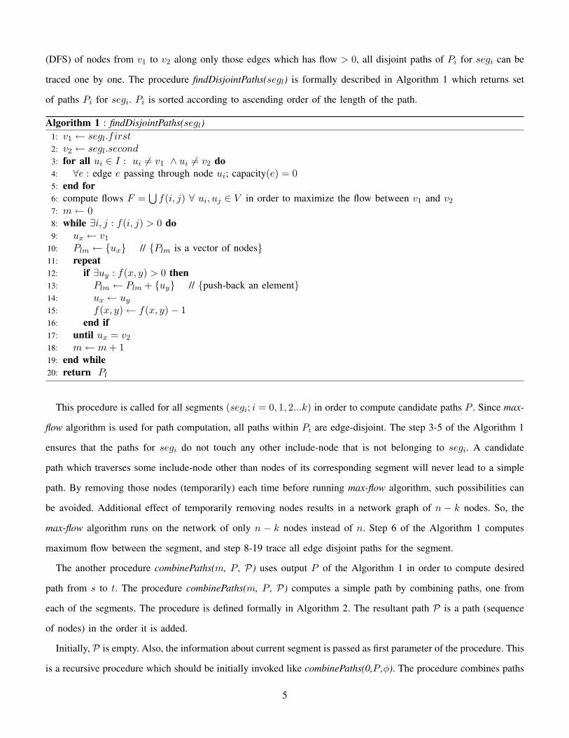
(DFS) of nodes from v1 to v2 along only those edges which has flow > 0, all disjoint paths of Pi for segi can be

traced one by one. The procedure findDisjointPaths(segl) is formally described in Algorithm 1 which returns set

of paths Pi for segi. Pi is sorted according to ascending order of the length of the path.

Algorithm 1 : findDisjointPaths(segl)1: v1 ← segl.first2: v2 ← segl.second3: for all ui ∈ I : ui 6= v1 ∧ ui 6= v2 do4: ∀e : edge e passing through node ui; capacity(e) = 05: end for6: compute flows F =

⋃f(i, j) ∀ ui, uj ∈ V in order to maximize the flow between v1 and v2

7: m← 08: while ∃i, j : f(i, j) > 0 do9: ux ← v1

10: Plm ← {ux} // {Plm is a vector of nodes}11: repeat12: if ∃uy : f(x, y) > 0 then13: Plm ← Plm + {uy} // {push-back an element}14: ux ← uy15: f(x, y)← f(x, y)− 116: end if17: until ux = v218: m← m+ 119: end while20: return Pl

This procedure is called for all segments (segi; i = 0, 1, 2...k) in order to compute candidate paths P . Since max-

flow algorithm is used for path computation, all paths within Pi are edge-disjoint. The step 3-5 of the Algorithm 1

ensures that the paths for segi do not touch any other include-node that is not belonging to segi. A candidate

path which traverses some include-node other than nodes of its corresponding segment will never lead to a simple

path. By removing those nodes (temporarily) each time before running max-flow algorithm, such possibilities can

be avoided. Additional effect of temporarily removing nodes results in a network graph of n − k nodes. So, the

max-flow algorithm runs on the network of only n − k nodes instead of n. Step 6 of the Algorithm 1 computes

maximum flow between the segment, and step 8-19 trace all edge disjoint paths for the segment.

The another procedure combinePaths(m, P , P) uses output P of the Algorithm 1 in order to compute desired

path from s to t. The procedure combinePaths(m, P , P) computes a simple path by combining paths, one from

each of the segments. The procedure is defined formally in Algorithm 2. The resultant path P is a path (sequence

of nodes) in the order it is added.

Initially, P is empty. Also, the information about current segment is passed as first parameter of the procedure. This

is a recursive procedure which should be initially invoked like combinePaths(0,P ,φ). The procedure combines paths

5

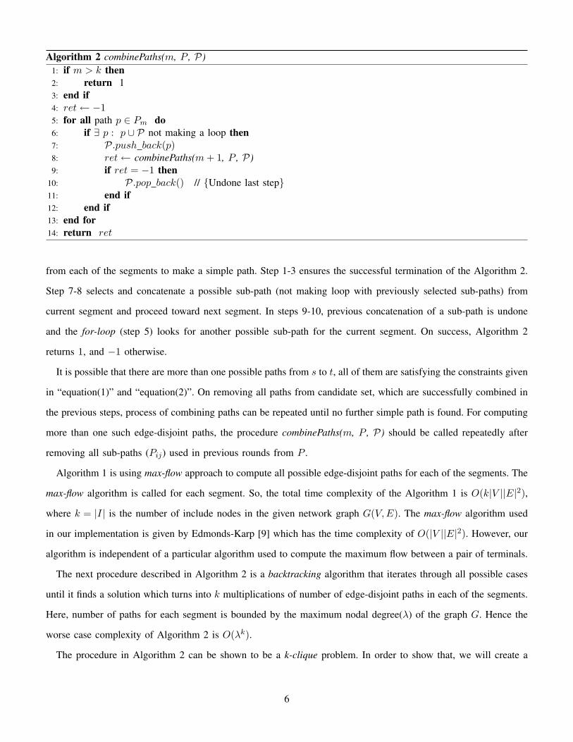
Algorithm 2 combinePaths(m, P , P)1: if m > k then2: return 13: end if4: ret← −15: for all path p ∈ Pm do6: if ∃ p : p ∪ P not making a loop then7: P.push back(p)8: ret← combinePaths(m+ 1, P , P)9: if ret = −1 then

10: P.pop back() // {Undone last step}11: end if12: end if13: end for14: return ret

from each of the segments to make a simple path. Step 1-3 ensures the successful termination of the Algorithm 2.

Step 7-8 selects and concatenate a possible sub-path (not making loop with previously selected sub-paths) from

current segment and proceed toward next segment. In steps 9-10, previous concatenation of a sub-path is undone

and the for-loop (step 5) looks for another possible sub-path for the current segment. On success, Algorithm 2

returns 1, and −1 otherwise.

It is possible that there are more than one possible paths from s to t, all of them are satisfying the constraints given

in “equation(1)” and “equation(2)”. On removing all paths from candidate set, which are successfully combined in

the previous steps, process of combining paths can be repeated until no further simple path is found. For computing

more than one such edge-disjoint paths, the procedure combinePaths(m, P , P) should be called repeatedly after

removing all sub-paths (Pij) used in previous rounds from P .

Algorithm 1 is using max-flow approach to compute all possible edge-disjoint paths for each of the segments. The

max-flow algorithm is called for each segment. So, the total time complexity of the Algorithm 1 is O(k|V ||E|2),

where k = |I| is the number of include nodes in the given network graph G(V,E). The max-flow algorithm used

in our implementation is given by Edmonds-Karp [9] which has the time complexity of O(|V ||E|2). However, our

algorithm is independent of a particular algorithm used to compute the maximum flow between a pair of terminals.

The next procedure described in Algorithm 2 is a backtracking algorithm that iterates through all possible cases

until it finds a solution which turns into k multiplications of number of edge-disjoint paths in each of the segments.

Here, number of paths for each segment is bounded by the maximum nodal degree(λ) of the graph G. Hence the

worse case complexity of Algorithm 2 is O(λk).

The procedure in Algorithm 2 can be shown to be a k-clique problem. In order to show that, we will create a

6

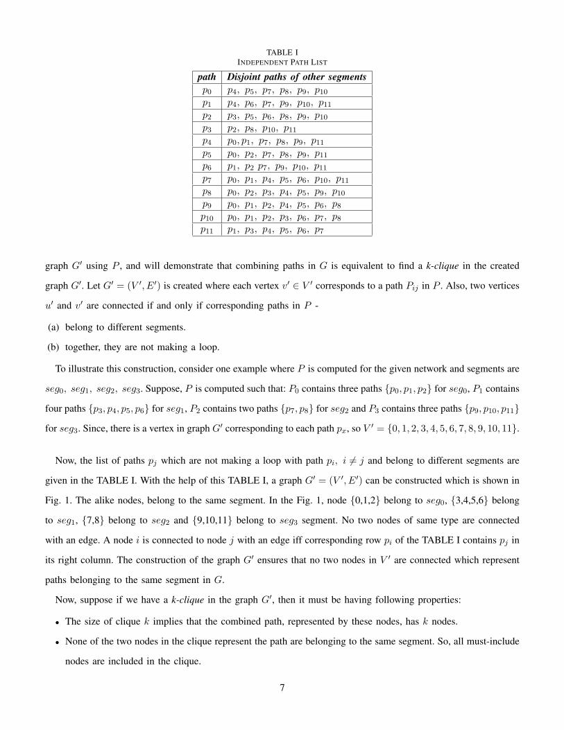
TABLE IINDEPENDENT PATH LIST

path Disjoint paths of other segmentsp0 p4, p5, p7, p8, p9, p10

p1 p4, p6, p7, p9, p10, p11

p2 p3, p5, p6, p8, p9, p10

p3 p2, p8, p10, p11

p4 p0, p1, p7, p8, p9, p11

p5 p0, p2, p7, p8, p9, p11

p6 p1, p2 p7, p9, p10, p11

p7 p0, p1, p4, p5, p6, p10, p11

p8 p0, p2, p3, p4, p5, p9, p10

p9 p0, p1, p2, p4, p5, p6, p8

p10 p0, p1, p2, p3, p6, p7, p8

p11 p1, p3, p4, p5, p6, p7

graph G′ using P , and will demonstrate that combining paths in G is equivalent to find a k-clique in the created

graph G′. Let G′ = (V ′, E′) is created where each vertex v′ ∈ V ′ corresponds to a path Pij in P . Also, two vertices

u′ and v′ are connected if and only if corresponding paths in P -

(a) belong to different segments.

(b) together, they are not making a loop.

To illustrate this construction, consider one example where P is computed for the given network and segments are

seg0, seg1, seg2, seg3. Suppose, P is computed such that: P0 contains three paths {p0, p1, p2} for seg0, P1 contains

four paths {p3, p4, p5, p6} for seg1, P2 contains two paths {p7, p8} for seg2 and P3 contains three paths {p9, p10, p11}

for seg3. Since, there is a vertex in graph G′ corresponding to each path px, so V ′ = {0, 1, 2, 3, 4, 5, 6, 7, 8, 9, 10, 11}.

Now, the list of paths pj which are not making a loop with path pi, i 6= j and belong to different segments are

given in the TABLE I. With the help of this TABLE I, a graph G′ = (V ′, E′) can be constructed which is shown in

Fig. 1. The alike nodes, belong to the same segment. In the Fig. 1, node {0,1,2} belong to seg0, {3,4,5,6} belong

to seg1, {7,8} belong to seg2 and {9,10,11} belong to seg3 segment. No two nodes of same type are connected

with an edge. A node i is connected to node j with an edge iff corresponding row pi of the TABLE I contains pj in

its right column. The construction of the graph G′ ensures that no two nodes in V ′ are connected which represent

paths belonging to the same segment in G.

Now, suppose if we have a k-clique in the graph G′, then it must be having following properties:

• The size of clique k implies that the combined path, represented by these nodes, has k nodes.

• None of the two nodes in the clique represent the path are belonging to the same segment. So, all must-include

nodes are included in the clique.

7

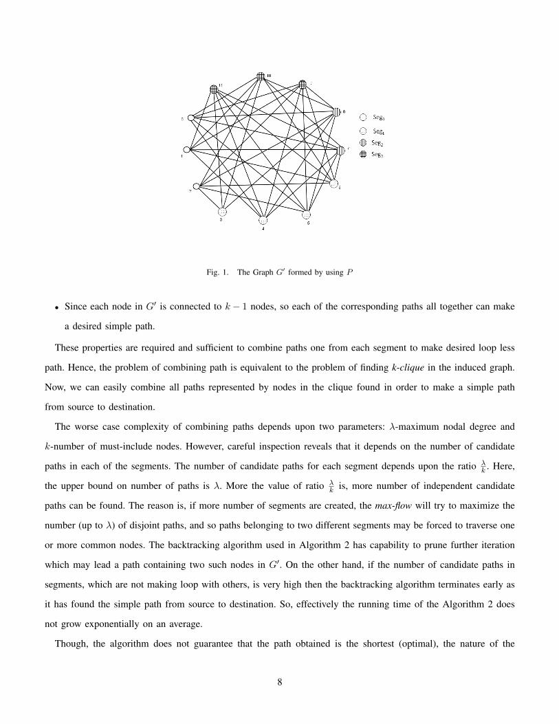
Fig. 1. The Graph G′ formed by using P

• Since each node in G′ is connected to k− 1 nodes, so each of the corresponding paths all together can make

a desired simple path.

These properties are required and sufficient to combine paths one from each segment to make desired loop less

path. Hence, the problem of combining path is equivalent to the problem of finding k-clique in the induced graph.

Now, we can easily combine all paths represented by nodes in the clique found in order to make a simple path

from source to destination.

The worse case complexity of combining paths depends upon two parameters: λ-maximum nodal degree and

k-number of must-include nodes. However, careful inspection reveals that it depends on the number of candidate

paths in each of the segments. The number of candidate paths for each segment depends upon the ratio λk . Here,

the upper bound on number of paths is λ. More the value of ratio λk is, more number of independent candidate

paths can be found. The reason is, if more number of segments are created, the max-flow will try to maximize the

number (up to λ) of disjoint paths, and so paths belonging to two different segments may be forced to traverse one

or more common nodes. The backtracking algorithm used in Algorithm 2 has capability to prune further iteration

which may lead a path containing two such nodes in G′. On the other hand, if the number of candidate paths in

segments, which are not making loop with others, is very high then the backtracking algorithm terminates early as

it has found the simple path from source to destination. So, effectively the running time of the Algorithm 2 does

not grow exponentially on an average.

Though, the algorithm does not guarantee that the path obtained is the shortest (optimal), the nature of the

8

algorithm results in near shortest possible paths which satisfy the constraint of including given set of nodes. The

max-flow computation uses shortest path for computing augmenting paths [11]. Also, we sort the paths in P

according to the hop-count. Further, the Algorithm 2 traverses nodes of G′, formed by using P , in increasing order

of index of nodes. Hence, the near-shortest possible path will be found first. If the Algorithm 2 is called second

time after removal of all nodes in G′ which belong to previous found paths, the next possible path between s and

t will not be shorter than the previous ones. In order to support this claim, we compared our result for smaller

networks with the results obtained by running K-shortest path algorithm repeatedly with incrementing the value of

K until desired path is obtained. Since the value of K required by K-shortest path algorithm is very large, it is

computationally not possible to get the optimal results for larger networks.

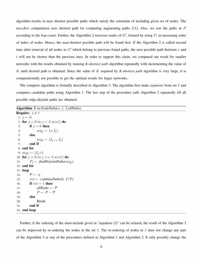
The complete algorithm is formally described in Algorithm 3. The algorithm first make segments from set I and

computes candidate paths using Algorithm 1. The last step of the procedure calls Algorithm 2 repeatedly till all

possible edge-disjoint paths are obtained.

Algorithm 3 incNodePaths(s, t, I ,allPaths)Require: s 6= t

1: j ← 02: for j = 0 to j < I.size() do3: if j = 0 then4: segj ← (s, Ij)5: else6: segj ← (Ij−1, Ij)7: end if8: end for9: segj ← (Ij , t)

10: for j = 0 to j <= I.size() do11: Pj ← findDisjointPaths(segj)12: end for13: loop14: P ← φ15: ret← combinePaths(0, P ,P)16: if ret = 1 then17: allPaths ← P18: P ← P − P19: else20: Break21: end if22: end loop

Further, if the ordering of the must-include given in “equation (2)” can be relaxed, the result of the Algorithm 3

can be improved by re-ordering the nodes in the set I . The re-ordering of nodes in I does not change any part

of the Algorithm 3 or any of the procedures defined in Algorithm 1 and Algorithm 2. It only possibly change the

9

relative ordering of the include nodes in the desired path. This pre-computation step can be done before calling the

Algorithm 3.

The re-ordering of include nodes can be done using simple algorithm such as depth first traversal. Let the set I ′

is the outcome of this process. Starting depth first traversal from s, suppose the node that is traversed first among

I is x1, then it should be placed first in say I ′. Now, restarting depth first traversal from x1, let the node x2 is

traversed first among I − I ′ then x2 should be placed next in I ′. Repeating the process until I − I ′ = φ results

in I ′ which contains all element of I but may be in different order. The new set I ′ of must-include nodes can be

used instead of I in Algorithm 3.

The motivation of Algorithm 1 is to find maximum number of candidates for each of the segments such that

each of the candidates is sharing the least number (0) of intermediate nodes with other candidates. And, the idea

behind re-arranging the order of must-include nodes using depth first traversal is to avoid making a segment with

nodes that are far apart. If the two nodes of the segment is nearer, the number of hops in the candidate paths for

the segment is lesser. Hence, the possibility of interfering of a candidate path with other candidates is decreased

and path combining process in Algorithm 2 becomes more successful.

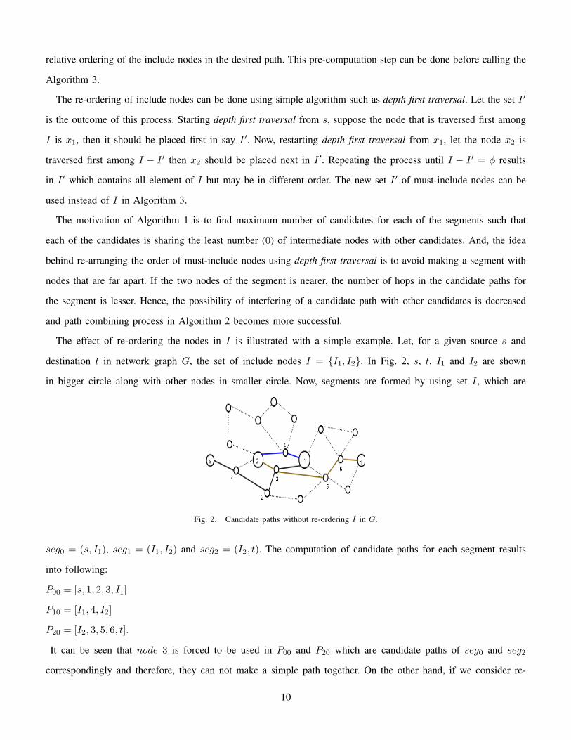
The effect of re-ordering the nodes in I is illustrated with a simple example. Let, for a given source s and

destination t in network graph G, the set of include nodes I = {I1, I2}. In Fig. 2, s, t, I1 and I2 are shown

in bigger circle along with other nodes in smaller circle. Now, segments are formed by using set I , which are

Fig. 2. Candidate paths without re-ordering I in G.

seg0 = (s, I1), seg1 = (I1, I2) and seg2 = (I2, t). The computation of candidate paths for each segment results

into following:

P00 = [s, 1, 2, 3, I1]

P10 = [I1, 4, I2]

P20 = [I2, 3, 5, 6, t].

It can be seen that node 3 is forced to be used in P00 and P20 which are candidate paths of seg0 and seg2

correspondingly and therefore, they can not make a simple path together. On the other hand, if we consider re-

10

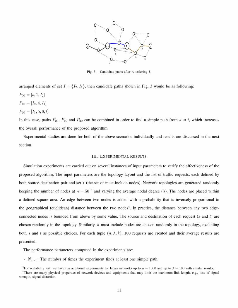
Fig. 3. Candidate paths after re-ordering I .

arranged elements of set I = {I2, I1}, then candidate paths shown in Fig. 3 would be as following:

P00 = [s, 1, I2]

P10 = [I2, 4, I1]

P20 = [I1, 5, 6, t].

In this case, paths P00, P10 and P20 can be combined in order to find a simple path from s to t, which increases

the overall performance of the proposed algorithm.

Experimental studies are done for both of the above scenarios individually and results are discussed in the next

section.

III. EXPERIMENTAL RESULTS

Simulation experiments are carried out on several instances of input parameters to verify the effectiveness of the

proposed algorithm. The input parameters are the topology layout and the list of traffic requests, each defined by

both source-destination pair and set I (the set of must-include nodes). Network topologies are generated randomly

keeping the number of nodes at n = 50 3 and varying the average nodal degree (λ). The nodes are placed within

a defined square area. An edge between two nodes is added with a probability that is inversely proportional to

the geographical (euclidean) distance between the two nodes4. In practice, the distance between any two edge-

connected nodes is bounded from above by some value. The source and destination of each request (s and t) are

chosen randomly in the topology. Similarly, k must-include nodes are chosen randomly in the topology, excluding

both s and t as possible choices. For each tuple (n, λ, k), 100 requests are created and their average results are

presented.

The performance parameters computed in the experiments are:

- Nsucc: The number of times the experiment finds at least one simple path.

3For scalability test, we have run additional experiments for larger networks up to n = 1000 and up to λ = 100 with similar results.4There are many physical properties of network devices and equipments that may limit the maximum link length, e.g., loss of signal

strength, signal distortion.

11

- Davg : The average number of edge disjoint paths found per request.

- Texp : Total experiment run time.

Nsucc represents the number of instances out of 100 for which the algorithm is able to find at least one path from

s to t that satisfies the must-include node constraint given in “equation (1)”. Davg represents the average number

of edge-disjoint paths that are found per request, accounting for all 100 experiments. Texp represents the average

execution time of the experiment for all 100 requests. Texp is the sum of the run time required by both Algorithm 1

and Algorithm 2. The suffix (W) denotes the result of the experiment without the reordering of I . The suffix (R)

denotes the result of the experiment with the reordering of I . All of the experiments are conducted on the same

hardware and software platform. The complete result is shown in the table II. In the following paragraphs, each of

the parameters are discussed one by one.

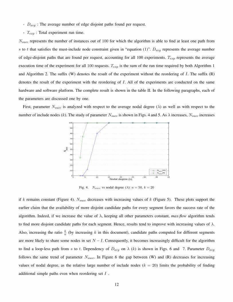
First, parameter Nsucc is analyzed with respect to the average nodal degree (λ) as well as with respect to the

number of include nodes (k). The study of parameter Nsucc is shown in Figs. 4 and 5. As λ increases, Nsucc increases

0 5 10 15 20 25 30 35 400

10

20

30

40

50

60

70

80

90

100

Nodal degree (λ)

N succ

Nsucc

(W)

Nsucc

(R)

Fig. 4. Nsucc vs nodal degree (λ): n = 50, k = 20

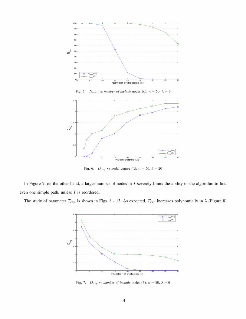
if k remains constant (Figure 4). Nsucc decreases with increasing values of k (Figure 5). These plots support the

earlier claim that the availability of more disjoint candidate paths for every segment favors the success rate of the

algorithm. Indeed, if we increase the value of λ, keeping all other parameters constant, max-flow algorithm tends

to find more disjoint candidate paths for each segment. Hence, results tend to improve with increasing values of λ.

Also, increasing the ratio kn (by increasing k in this document), candidate paths computed for different segments

are more likely to share some nodes in set N − I . Consequently, it becomes increasingly difficult for the algorithm

to find a loop-less path from s to t. Dependency of Davg on λ (k) is shown in Figs. 6 and 7. Parameter Davg

follows the same trend of parameter Nsucc. In Figure 6 the gap between (W) and (R) decreases for increasing

values of nodal degree, as the relative large number of include nodes (k = 20) limits the probability of finding

additional simple paths even when reordering set I .

12

TABLE IIEXPERIMENT RESULTS

N λ k Nsucc(W ) Davg(W ) Texp(W ) Nsucc(R) Davg(R) Texp(R)50 3 20 0 0 13 34 0.34 1550 4 20 0 0 18 74 0.74 2150 6 20 12 0.12 23 100 1 2950 10 20 80 0.8 37 100 1.15 4350 15 20 100 1 58 100 1.78 6550 20 20 100 1.51 87 100 1.97 9550 25 20 100 1.83 119 100 2.13 13650 30 20 100 1.96 160 100 2.23 19450 35 20 100 2.12 211 100 2.35 26450 40 20 100 2.2 272 100 2.36 31250 6 2 100 2.71 6 100 3.12 750 6 5 100 1.74 12 100 2.13 1450 6 10 96 1.03 17 100 1.43 2050 6 15 53 0.53 21 100 1.02 2650 6 20 12 0.12 23 100 1 2950 6 25 1 0.01 25 98 0.98 3250 6 30 0 0 26 93 0.93 3150 6 35 0 0 24 83 0.83 3050 6 40 0 0 23 63 0.63 29250 6 10 100 1.63 79 100 2.28 79250 10 10 100 2.7 117 100 3.78 130250 15 10 100 3.87 162 100 5.91 180250 25 10 100 5.31 269 100 8.34 302250 6 25 94 1 92 100 1.43 93250 10 25 100 1.32 249 100 2.13 281250 15 25 100 2 347 100 3.04 376250 25 25 100 3.22 572 100 4.56 621250 50 25 100 5.74 1377 100 7.09 1402250 50 50 100 3 2333 100 3.88 2410250 100 50 100 4 7603 100 4.73 8012500 10 10 100 3.02 233 100 3.83 431500 10 25 100 1.87 519 100 2.78 827500 15 10 100 4.66 313 100 5.34 461500 15 25 100 2.81 705 100 3.89 898500 25 100 100 1 3502 100 2 3787500 25 10 100 7.25 484 100 7.76 682500 25 25 100 4.39 1100 100 4.87 1289500 25 50 100 2.53 2044 100 3.23 2296500 50 100 100 2.16 8661 100 3.1 8899500 50 200 100 1 12273 100 2 13225500 50 25 100 7.56 2500 100 8.12 2760500 50 50 100 4.53 4659 100 5.34 4950500 6 10 100 1.9 163 100 2 310500 6 25 99 1 368 100 1.68 588500 75 150 100 2 20476 100 3 20913500 75 300 85 1 25708 100 1.74 34749500 75 50 100 6.11 8773 100 6.58 8474

TABLE IIIEXPERIMENT RESULTS FOR LARGE NETWORKS

N λ k Nsucc(W ) Davg(W ) Texp(W ) Nsucc(R) Davg(R) Texp(R)1000 5 10 100 1.89 257 100 2 670.9531000 10 20 100 2.94 963 100 3.2 1321.671000 25 50 100 3.92 4851 100 4.5 5231.581000 50 50 100 6.85 8645 100 7.2 10221.41000 100 100 100 6.14 70032 100 6.8 60232.7

13

0 5 10 15 20 25 30 35 400

10

20

30

40

50

60

70

80

90

100

Number of includes (k)

N succ

Nsucc

(W)

Nsucc

(R)

Fig. 5. Nsucc vs number of include nodes (k): n = 50, λ = 6

0 5 10 15 20 25 30 35 400

0.5

1

1.5

2

2.5

Nodal degree (λ)

D avg

Davg

(W)

Davg

(R)

Fig. 6. Davg vs nodal degree (λ): n = 50, k = 20

In Figure 7, on the other hand, a larger number of nodes in I severely limits the ability of the algorithm to find

even one simple path, unless I is reordered.

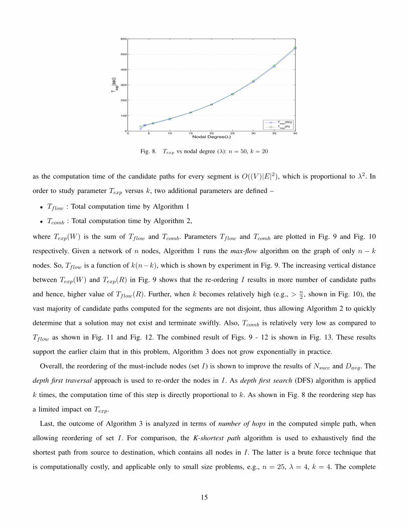
The study of parameter Texp is shown in Figs. 8 - 13. As expected, Texp increases polynomially in λ (Figure 8)

0 5 10 15 20 25 30 35 400

0.5

1

1.5

2

2.5

3

3.5

Number of includes (k)

D avg

Davg

(W)

Davg

(R)

Fig. 7. Davg vs number of include nodes (k): n = 50, λ = 6

14

0 5 10 15 20 25 30 35 400

100

200

300

400

500

600

Nodal Degree(!)

T exp(se

c)

Texp(W))Texp(R)

Fig. 8. Texp vs nodal degree (λ): n = 50, k = 20

as the computation time of the candidate paths for every segment is O((V )|E|2), which is proportional to λ2. In

order to study parameter Texp versus k, two additional parameters are defined –

• Tflow : Total computation time by Algorithm 1

• Tcomb : Total computation time by Algorithm 2,

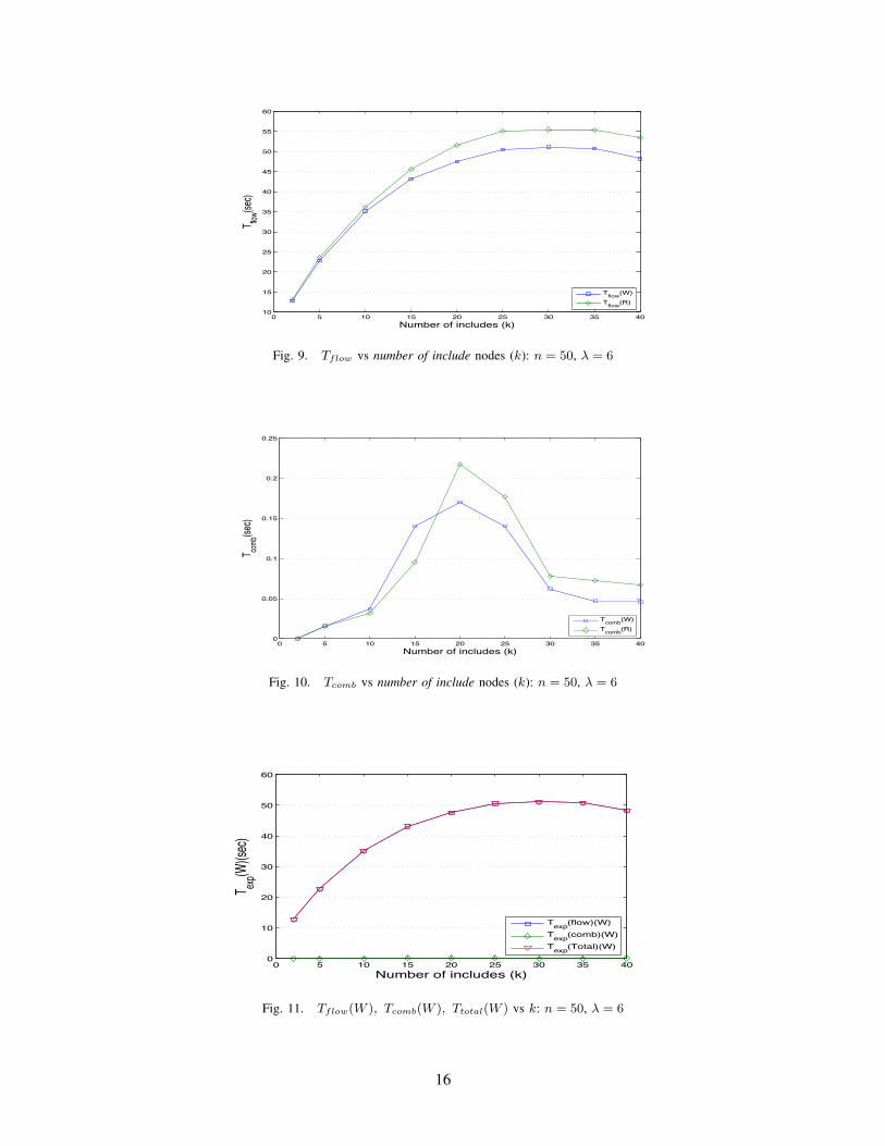
where Texp(W ) is the sum of Tflow and Tcomb. Parameters Tflow and Tcomb are plotted in Fig. 9 and Fig. 10

respectively. Given a network of n nodes, Algorithm 1 runs the max-flow algorithm on the graph of only n − k

nodes. So, Tflow is a function of k(n−k), which is shown by experiment in Fig. 9. The increasing vertical distance

between Texp(W ) and Texp(R) in Fig. 9 shows that the re-ordering I results in more number of candidate paths

and hence, higher value of Tflow(R). Further, when k becomes relatively high (e.g., > n2 , shown in Fig. 10), the

vast majority of candidate paths computed for the segments are not disjoint, thus allowing Algorithm 2 to quickly

determine that a solution may not exist and terminate swiftly. Also, Tcomb is relatively very low as compared to

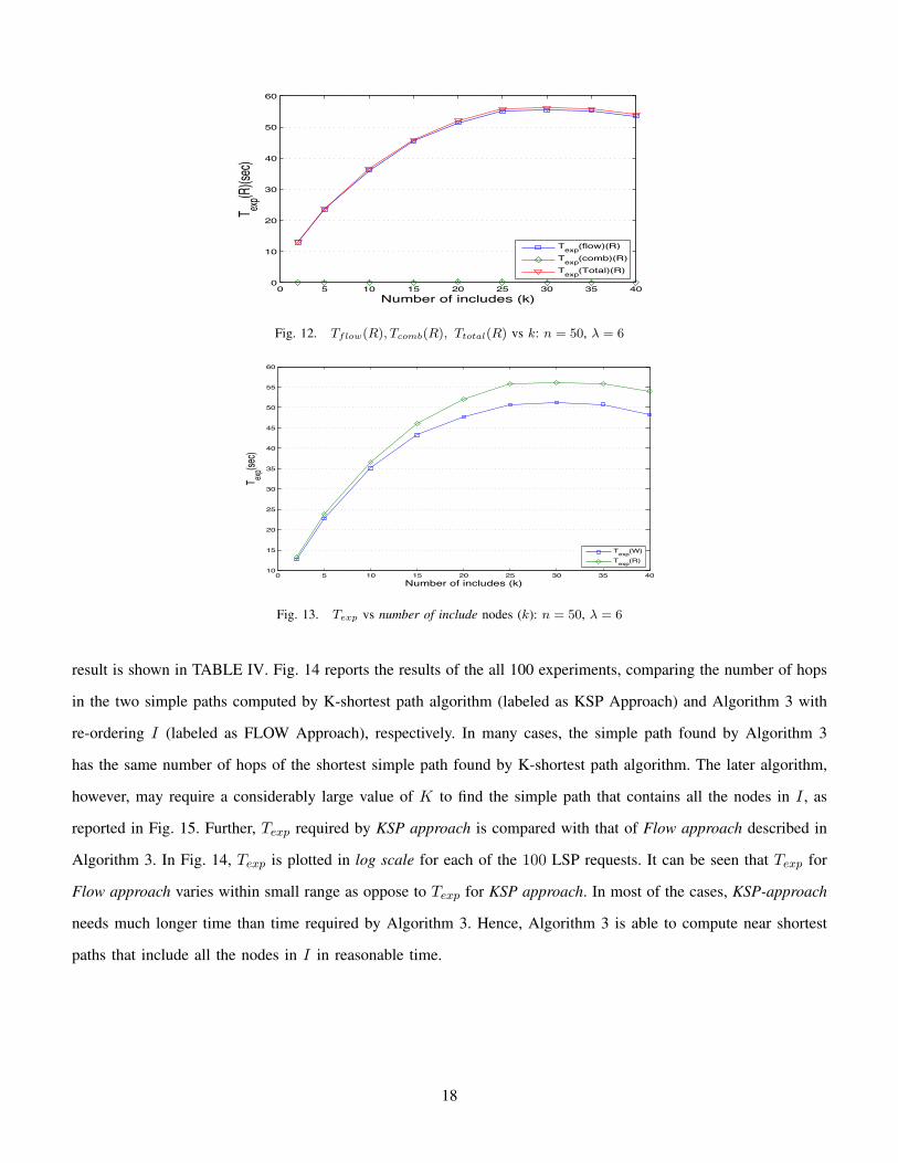
Tflow as shown in Fig. 11 and Fig. 12. The combined result of Figs. 9 - 12 is shown in Fig. 13. These results

support the earlier claim that in this problem, Algorithm 3 does not grow exponentially in practice.

Overall, the reordering of the must-include nodes (set I) is shown to improve the results of Nsucc and Davg. The

depth first traversal approach is used to re-order the nodes in I . As depth first search (DFS) algorithm is applied

k times, the computation time of this step is directly proportional to k. As shown in Fig. 8 the reordering step has

a limited impact on Texp.

Last, the outcome of Algorithm 3 is analyzed in terms of number of hops in the computed simple path, when

allowing reordering of set I . For comparison, the K-shortest path algorithm is used to exhaustively find the

shortest path from source to destination, which contains all nodes in I . The latter is a brute force technique that

is computationally costly, and applicable only to small size problems, e.g., n = 25, λ = 4, k = 4. The complete

15

0 5 10 15 20 25 30 35 4010

15

20

25

30

35

40

45

50

55

60

Number of includes (k)

T flow(se

c)

Tflow(W)Tflow(R)

Fig. 9. Tflow vs number of include nodes (k): n = 50, λ = 6

0 5 10 15 20 25 30 35 400

0.05

0.1

0.15

0.2

0.25

Number of includes (k)

T comb

(sec)

Tcomb(W)Tcomb(R)

Fig. 10. Tcomb vs number of include nodes (k): n = 50, λ = 6

0 5 10 15 20 25 30 35 400

10

20

30

40

50

60

Number of includes (k)

T exp(W

)(sec)

Texp(flow)(W)Texp(comb)(W)Texp(Total)(W)

Fig. 11. Tflow(W ), Tcomb(W ), Ttotal(W ) vs k: n = 50, λ = 6

16

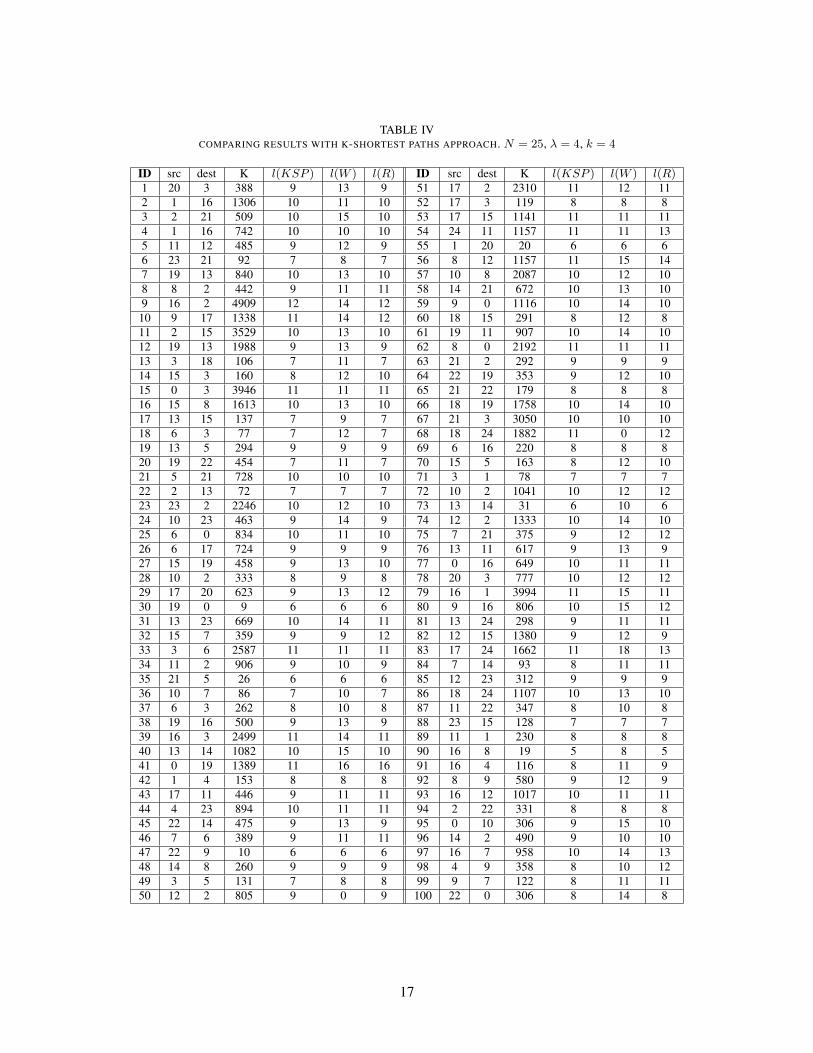
TABLE IVCOMPARING RESULTS WITH K-SHORTEST PATHS APPROACH. N = 25, λ = 4, k = 4

ID src dest K l(KSP ) l(W ) l(R) ID src dest K l(KSP ) l(W ) l(R)1 20 3 388 9 13 9 51 17 2 2310 11 12 112 1 16 1306 10 11 10 52 17 3 119 8 8 83 2 21 509 10 15 10 53 17 15 1141 11 11 114 1 16 742 10 10 10 54 24 11 1157 11 11 135 11 12 485 9 12 9 55 1 20 20 6 6 66 23 21 92 7 8 7 56 8 12 1157 11 15 147 19 13 840 10 13 10 57 10 8 2087 10 12 108 8 2 442 9 11 11 58 14 21 672 10 13 109 16 2 4909 12 14 12 59 9 0 1116 10 14 10

10 9 17 1338 11 14 12 60 18 15 291 8 12 811 2 15 3529 10 13 10 61 19 11 907 10 14 1012 19 13 1988 9 13 9 62 8 0 2192 11 11 1113 3 18 106 7 11 7 63 21 2 292 9 9 914 15 3 160 8 12 10 64 22 19 353 9 12 1015 0 3 3946 11 11 11 65 21 22 179 8 8 816 15 8 1613 10 13 10 66 18 19 1758 10 14 1017 13 15 137 7 9 7 67 21 3 3050 10 10 1018 6 3 77 7 12 7 68 18 24 1882 11 0 1219 13 5 294 9 9 9 69 6 16 220 8 8 820 19 22 454 7 11 7 70 15 5 163 8 12 1021 5 21 728 10 10 10 71 3 1 78 7 7 722 2 13 72 7 7 7 72 10 2 1041 10 12 1223 23 2 2246 10 12 10 73 13 14 31 6 10 624 10 23 463 9 14 9 74 12 2 1333 10 14 1025 6 0 834 10 11 10 75 7 21 375 9 12 1226 6 17 724 9 9 9 76 13 11 617 9 13 927 15 19 458 9 13 10 77 0 16 649 10 11 1128 10 2 333 8 9 8 78 20 3 777 10 12 1229 17 20 623 9 13 12 79 16 1 3994 11 15 1130 19 0 9 6 6 6 80 9 16 806 10 15 1231 13 23 669 10 14 11 81 13 24 298 9 11 1132 15 7 359 9 9 12 82 12 15 1380 9 12 933 3 6 2587 11 11 11 83 17 24 1662 11 18 1334 11 2 906 9 10 9 84 7 14 93 8 11 1135 21 5 26 6 6 6 85 12 23 312 9 9 936 10 7 86 7 10 7 86 18 24 1107 10 13 1037 6 3 262 8 10 8 87 11 22 347 8 10 838 19 16 500 9 13 9 88 23 15 128 7 7 739 16 3 2499 11 14 11 89 11 1 230 8 8 840 13 14 1082 10 15 10 90 16 8 19 5 8 541 0 19 1389 11 16 16 91 16 4 116 8 11 942 1 4 153 8 8 8 92 8 9 580 9 12 943 17 11 446 9 11 11 93 16 12 1017 10 11 1144 4 23 894 10 11 11 94 2 22 331 8 8 845 22 14 475 9 13 9 95 0 10 306 9 15 1046 7 6 389 9 11 11 96 14 2 490 9 10 1047 22 9 10 6 6 6 97 16 7 958 10 14 1348 14 8 260 9 9 9 98 4 9 358 8 10 1249 3 5 131 7 8 8 99 9 7 122 8 11 1150 12 2 805 9 0 9 100 22 0 306 8 14 8

17

0 5 10 15 20 25 30 35 400

10

20

30

40

50

60

Number of includes (k)

T exp(R)

(sec)

Texp(flow)(R)Texp(comb)(R)Texp(Total)(R)

Fig. 12. Tflow(R), Tcomb(R), Ttotal(R) vs k: n = 50, λ = 6

0 5 10 15 20 25 30 35 4010

15

20

25

30

35

40

45

50

55

60

Number of includes (k)

T exp(se

c)

Texp(W)Texp(R)

Fig. 13. Texp vs number of include nodes (k): n = 50, λ = 6

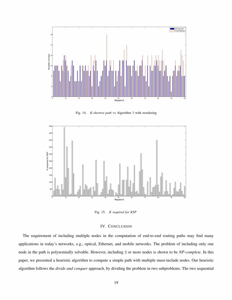
result is shown in TABLE IV. Fig. 14 reports the results of the all 100 experiments, comparing the number of hops

in the two simple paths computed by K-shortest path algorithm (labeled as KSP Approach) and Algorithm 3 with

re-ordering I (labeled as FLOW Approach), respectively. In many cases, the simple path found by Algorithm 3

has the same number of hops of the shortest simple path found by K-shortest path algorithm. The later algorithm,

however, may require a considerably large value of K to find the simple path that contains all the nodes in I , as

reported in Fig. 15. Further, Texp required by KSP approach is compared with that of Flow approach described in

Algorithm 3. In Fig. 14, Texp is plotted in log scale for each of the 100 LSP requests. It can be seen that Texp for

Flow approach varies within small range as oppose to Texp for KSP approach. In most of the cases, KSP-approach

needs much longer time than time required by Algorithm 3. Hence, Algorithm 3 is able to compute near shortest

paths that include all the nodes in I in reasonable time.

18

0 10 20 30 40 50 60 70 80 90 1004

6

8

10

12

14

16

Request Id

Num

ber o

f hop

s

KSP ApproachFLOW Approach

Fig. 14. K-shortest path vs Algorithm 3 with reordering

0 10 20 30 40 50 60 70 80 90 1000

500

1000

1500

2000

2500

3000

3500

4000

4500

5000

Request Id

K re

quire

d fo

r KS

P

Fig. 15. K required for KSP

IV. CONCLUSION

The requirement of including multiple nodes in the computation of end-to-end routing paths may find many

applications in today’s networks, e.g., optical, Ethernet, and mobile networks. The problem of including only one

node in the path is polynomially solvable. However, including 2 or more nodes is shown to be NP-complete. In this

paper, we presented a heuristic algorithm to compute a simple path with multiple must-include nodes. Our heuristic

algorithm follows the divide and conquer approach, by dividing the problem in two subproblems. The two sequential

19

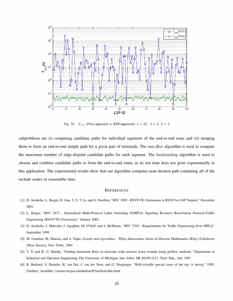
Fig. 16. Texp (Flow-approach vs KSP-approach); n = 25, λ = 4, k = 4

subproblems are (i) computing candidate paths for individual segments of the end-to-end route and (ii) merging

them to form an end-to-end simple path for a given pair of terminals. The max-flow algorithm is used to compute

the maximum number of edge-disjoint candidate paths for each segment. The backtracking algorithm is used to

choose and combine candidate paths to form the end-to-end route, as its run time does not grow exponentially in

this application. The experimental results show that our algorithm computes near-shortest path containing all of the

include nodes in reasonable time.

REFERENCES

[1] D. Awduche, L. Berger, D. Gan, V. S. T. Li, and G. Swallow, “RFC 3209 - RSVP-TE: Extensions to RSVP for LSP Tunnels,” December

2001.

[2] L. Berger, “RFC 3473 - Generalized Multi-Protocol Label Switching (GMPLS) Signaling Resource ReserVation Protocol-Traffic

Engineering (RSVP-TE) Extensions,” January 2003.

[3] D. Awduche, J. Malcolm, J. Agogbua, M. O’Dell, and J. McManus, “RFC 2702 - Requirements for Traffic Engineering Over MPLS,”

September 1999.

[4] M. Gondran, M. Minoux, and S. Vajda, Graphs and algorithms. Wiley-Interscience Series in Discrete Mathematics.Wiley (Chichester

[West Sussex], New York), 1984.

[5] T. Yi and K. G. Murthy, “Finding maximum flows in networks with nonzero lower bounds using preflow methods,” Department of

Indusrtial and Operaion Engineering The University of Michigan Ann Arbor, MI 48109-2117, Tech. Rep., July 1991.

[6] R. Burkard, V. Deineko, R. van Dal, J. van der Veen, and G. Woeginger, “Well-solvable special cases of the tsp: A survey,” 1995.

[Online]. Available: citeseer.ist.psu.edu/burkard95wellsolvable.html

20

[7] E. L. Gilmore, P.C. and D. Shmoys, “Well-solved special cases,” 1985, in E.L. Lawler, J.K. Lenstra, A.H.G. Rinnooy-Kan and D.B.

Shmoys (eds.), Chapter 4 in The Traveling Salesman Problem: a Guided Tour of Combinatorial Optimization. Wiley: Chichester, pp.

87-144.

[8] H. J. Miller and S.-L. Shaw, Geographic Information Systems for Transportation: Principles and Applications. Oxford University

Press US, 2001.

[9] J. Edmonds and R. M. Karp, Theoretical Improvements in Algorithmic Efficiency for Network Flow Problems, New York, NY, USA,

1972.

[10] E. de Queirs Vieira Martins and M. M. B. Pascoal, “A new implementation of yen’s ranking loopless paths algorithm.” 4OR, vol. 1,

no. 2, pp. 121–133, 2003.

[11] T. H. Cormen, C. E. Leiserson, R. L. Rivest, and C. Stein, Introduction to Algorithms, Second Edition. The MIT Press, September

2001.

21