transportation options in a carbon-constrained world: hybrids, plug-in hybrids … ·...

*Corresponding author. Tel.:703-778-3122; fax: 703-212-4898 E-mail address: [email protected]

This paper published in the International Journal of Hydrogen Energy 34 (2009) 9279-9296 doi:10.1016/j.ijhydene.2009.09.058

Transportation Options in a Carbon-constrained World: Hybrids, Plug-in Hybrids, Biofuels, Fuel Cell Electric Vehicles,

and Battery Electric Vehicles C. E. (Sandy) Thomas*

H2Gen Innovations, Inc., Alexandria, Virginia, 22304, USA

Abstract

Multiple alternative vehicle and fuel options are being proposed to alleviate the threats of climate change, urban air pollution, and oil dependence caused by the transportation sector. We report here on the results from an extensive computer model developed over the last decade to simulate and compare the societal benefits of deploying various alternative transportation options including hybrid electric vehicles and plug-in hybrids fueled by gasoline, diesel fuel, natural gas, and ethanol, and all-electric vehicles powered by either batteries or fuel cells. These simulations compare the societal benefits over a 100-year time horizon of each vehicle/fuel combination in terms of reduced local air pollution, greenhouse gas pollution, and oil consumption compared to gasoline cars. The model demonstrates that partially electrified vehicles such as hybrids and plug-in hybrids will appreciably cut greenhouse gas pollution and oil consumption, particularly if biofuels such as cellulosic ethanol can displace a large amount of gasoline. But if we are to achieve an 80% reduction in greenhouse gases below 1990 levels, eliminate most oil imports and most urban air pollution, then society must transition to all-electric vehicles powered by some combination of fuel cells and batteries. We cannot achieve our transportation sector goals if most vehicles still rely on internal combustion engines for some of their motive power. We conclude that society must rely on a portfolio of alternative vehicles to achieve our societal objectives, beginning with hybrids, plug-in hybrids, biofuels, and transitioning to all-electric fuel cell and battery electric vehicles over time. Keywords:

Battery electric vehicles Fuel cell electric vehicles Hydrogen infrastructure Plug-in hybrids Greenhouse gases Electric vehicles Energy security

Dynamic simulation

Transportation Options in a Carbon-Constrained World

C.E. Thomas of 22 Int. J. of Hydrogen Energy 34 (2009) 9279-9296

Nomenclature/Acronyms:

AER all electric range GREET Greenhouse gases, Regulated Emissions and Energy use in Transportation (an Argonne National Laboratory computer program)

CCS carbon capture and storage LDV light duty vehicle (includes both passenger cars and light duty trucks)

CIDI compression ignition, direct injection NG natural gas

CO carbon monoxide NGV natural gas vehicle

DOE the United States Department of Energy

NOx nitrous oxides

HEV hybrid electric vehicle (a vehicle with an internal combustion engine and an electric traction motor)

NRC National Research Council

ICV internal combustion vehicle NRDC Natural Resources Defense Council

EIA Energy Information Administration (part of the DOE)

PM-2.5 particulate matter less than 2.5 microns in size

EPA Environmental Protection Agency PM-10 particulate matter less than 10 microns in size EPRI Electric Power Research Institute SI spark ignition

FC fuel cell SOx sulfur oxides

FCEV fuel cell electric vehicle VMT vehicle miles traveled

PFCEV plug-in fuel cell electric vehicle VOC volatile organic compounds

PHEV plug-in hybrid electric vehicle WECC Western Electricity Coordinating Council GHG greenhouse gases

1. Introduction

The transportation sector accounts for 28% of all US greenhouse gas emissions, 34% of all carbon dioxide emissions, 36% to 78% of the main ingredients of urban air pollution,1 and 68% of all oil consumption [1]. Clearly the monoculture of petroleum-based transportation 2 must change if we are to achieve our societal goals of an 80% reduction in greenhouse gas emissions below 1990 levels, substantially reduced dependence on imported petroleum and minimal urban air pollution in the decades ahead. Several options have been proposed for curtailing our addiction to oil, including both alternative vehicles and different fuels. The alternative vehicle options considered here all include some degree of electrification of the propulsion system. Hybrid electric vehicles (HEVs) are already on the road that add an electric traction motor and battery bank to a smaller version of the existing internal combustion engine to provide two sources of motive power. The next option under consideration is the plug-in hybrid electric vehicle

1 In 2006, transportation generated 35.5% of volatile organic compounds (VOCs), 58.3% of nitrous oxides (NOx), and 77.6% of carbon monoxide (CO) [1]. In addition, since much of this pollution is released in urban areas in close proximity to people, the health impact of transportation pollution may be higher than these percentages would indicate. 2 In 2007, petroleum supplied 95.8% of all US transportation energy [1]

(PHEV) that has batteries that can be charged from the grid while parked, so some gasoline use is replaced with electricity. The final step in this electrification evolution is to eliminate the internal combustion engine, resulting in an all-electric vehicle. The two all-electric vehicles under consideration are the fuel cell electric vehicle (FCEV) powered by hydrogen3 and the battery electric vehicle (BEV) that would depend exclusively on the electrical grid for all its energy. Alternatives to gasoline analyzed in this report include other fossil fuels such as diesel and natural gas that are not sustainable in the long term, and non-fossil fuels such as cellulosic ethanol (as a surrogate for other biomass-derived fuels such as butanol or biodiesel), hydrogen, and electricity, all of which could be produced sustainably in the future. Several organizations have analyzed the static performance of a set of alternative vehicles in terms of some combination of urban air pollution, greenhouse gas emissions, costs, and oil consumption, typically at one or two fixed periods of time. A 2001 report by General Motors supported by the Argonne National Laboratory

3 We assume here that all fuel cell electric vehicles utilize batteries or other energy storage devices such as ultracapacitors to provide peak power augmentation and also to capture some regenerative braking energy; some analysts call this type of fuel cell a “hybrid,” in the sense that it has both the fuel cell and a battery to provide electricity to the motor. But we reserve the term “hybrid” here to refer to a vehicle with both an internal combustion engine and an electric traction motor to generate motive power.



and three oil companies tabulated the GHGs for a combination of 30 fuel pathways and 15 different vehicles for the 2010 time period [2]. GM and Argonne later updated this projection to include urban air emissions, but again for a single fixed year (2016) [3]. These GM reports did not include plug-in hybrids or battery EVs. The European community analyzed the greenhouse gases from a wide variety of fuels and vehicles (again excluding plug-in hybrids and battery EVs) for the “2010 and beyond” time period [4]. Kromer and Heywood at MIT [5, 6] estimated the fuel economies, GHGs, and incremental costs for future advanced ICVs, hybrids, plug-in hybrids, and all-electric vehicles powered by either batteries or fuel cells in the year 2030. These static assessments at a fixed point in time are valuable, and we have used some of their results to benchmark several assumptions used in this study. To fully characterize an evolving transportation sector, however, we need a dynamic model to capture the impact of multiple parameters that are all changing gradually over time, including:

• Alternative vehicle and alternative fuel market penetration over time

• Improving fuel economy of the baseline gasoline vehicles and the alternative vehicles over time

• Increasing vehicle miles traveled (VMT) over time

• Changing sources of hydrogen over time as we move to more renewable hydrogen

• Changing sources of electricity over time as society begins reducing the carbon footprint of electrical generation

Some organizations have created dynamic models for a sub-set of alternative vehicles over time periods extending to 2030 or to 2050. The Electric Power Research Institute and the Natural Resources Defense Council analyzed the impact of adding gasoline hybrids and gasoline plug-in hybrids as a function of time out to 2030 [7]. However, they did not analyze either BEVs or FCEVs. The National Research Council conducted two dynamic assessments, one in 2004 [8] and one in 2008 [9], analyzing the impact of alternative vehicles to 2050. But the NRC did not evaluate plug-in hybrids, battery EVs or natural gas vehicles, and they did not analyze urban air pollution or externality costs. Proponents of NGVs, BEVs and PHEVs could speculate that these options might have faired better than the advanced ICVs, HEVs or FCEVs had they been analyzed by the NRC.

2. Transportation sector goals

We began our process by defining three major societal goals for the light duty vehicle (LDV) transportation sector. The ideal passenger car fleet would eventually:

• Reduce greenhouse gas pollution to 80% below 1990 levels

• Eliminate virtually all controllable urban air criteria pollutants

• Achieve “quasi-energy independence”, defined as reducing light duty vehicle oil consumption to such a level that US domestic oil production plus oil imports from only the American hemisphere could satisfy all non-transportation petroleum needs plus a small fraction of LDV transportation fuels in a crisis4.

Achieving these goals could take many decades. We have therefore extended our simulation over the entire 21st century to give time for significant market penetration of the alternative vehicles and also to give time to reduce the carbon footprints of electricity and hydrogen without extraordinary economic stress on society to make these changes. We have also evaluated the full range of leading contender alternative vehicles and fuels, so that readers can assess each option under a common set of assumptions.

3. Simulation methodology

The Argonne National Laboratory GREET 1.8a Excel spreadsheet model developed by Michael Wang et al. [10] was used to estimate oil consumption, greenhouse gas and urban air pollution (VOCs, NOx, CO, SOx, PM-2.5, and PM-10) for each vehicle/fuel combination. We modified some of the GREET input parameters over time to reflect the changing methods of producing ethanol, hydrogen, and electricity assuming that carbon constraints are implemented. Four other Excel spreadsheets were developed to address various issues and to construct a century long simulation of the societal impact of alternative vehicles and fuels:

1. GREET Extension Model. This Excel program extends the GREET time horizon in ten-year increments from 2020 (the last time period in the standard GREET1.8a model) to 2100. A computer macro was written to calculate the environmental impacts for each set of input

4 In normal times foreign oil will always be less expensive than domestic petroleum, barring wars or embargoes, so we would for economic reasons continue to consume imported oil just as we use many other foreign materials in our global economy. But with the introduction of higher fuel economy vehicles and the substitution of sufficient non-petroleum transportation fuels, we could substantially alleviate the impact of major oil disruptions in future crises.



parameters in ten-year increments, taking into account the changing parameters over time.

2. Market Penetration Model. This model simulates the gradual market penetration of alternative vehicles and fuels over the century and tabulates societal costs resulting from urban air pollution, greenhouse gas pollution, and oil consumption.

3. Marginal Grid Mix Model. This model evaluates the likely marginal grid mix for a given average combination of electrical generators for both the US as a whole and for the cleaner West Coast grid composition, taking into account economic dispatch whereby the generators with lowest operating cost are run as baseload, and generators with more expensive operating costs are run as peaking plants. This model averages over a range of nominal daily grid consumption demand profiles, and applies a 24-hour weighting function from EPRI [7] to simulate PHEV battery charging with emphasis on night-time charging to take advantage of excess (and low-cost) off-peak grid capacity.

4. Electric Vehicle Model. This model calculates the effects of mass compounding due to extra battery mass for PHEVs and particularly BEVs, and calculates the necessary electricity to run these vehicles over realistic vehicle drive cycles. This model was initially developed in the mid-1990’s under a DOE/Ford contract on hydrogen and FCEVs [11].

4. Key model assumptions

4.1. Vehicle/fuel combinations analyzed

We considered eight types of vehicle and six different fuels and analyzed in detail 15 different alternative vehicle/fuel combinations plus the gasoline ICV reference case (Table 1). These alternatives represent

vehicle/fuel combinations that have the best chance (or are being promoted as having a good chance) of contributing toward our transportation goals of reduced environmental and oil footprints. The model generates a 100-year projection of GHGs, oil imports, urban air pollution and total societal costs for each of these vehicle/fuel combinations. Space does not permit the full presentation of all these data, so we have concentrated our results on the four primary vehicle/fuel combinations designated with a “P” in Table 1; these are the primary options being pursued by the major automobile companies or, in the case of ethanol, promoted by other organizations:

• Gasoline-powered hybrid electric vehicles • Gasoline-powered plug-in hybrid electric

vehicles • Ethanol-powered plug-in hybrid electric vehicles • Hydrogen-powered fuel cell electric vehicles

Within some fuel categories, we show only the best options. For example, the plug-in hybrid running on ethanol provides the greatest reduction in oil import and GHG footprint, so we do not show dynamic details of either the ethanol ICV or the ethanol HEV. Similarly, the hydrogen plug-in FCEV (PFCEV) in this model produces more GHGs than the non-plug in version5, so we do not show the detailed 100-year data for the hydrogen PFCEV. In addition to these four main options being actively developed by most automobile companies, several other organizations or individuals are promoting hydrogen-powered ICE HEVs, natural gas vehicles and full-range all-electric battery vehicles. We have therefore included some results for these options in the results section.

5 The hydrogen plug-in FCEV has slightly higher GHGs than the non-plug-in FCEV over most of the century since the hydrogen production from natural gas starts out with lower GHGs than the grid, and the “greening” of the existing (mostly coal-based) electrical grid takes longer than the “greening” of hydrogen production with the assumptions used here.

Table 1 – Vehicle/fuel combinations analyzed in this report

Fuel: SI ICV CIDI HEV

CIDI PHEV

IC HEV

IC PHEV

FCEV PFCEV BEV

Gasoline Ref P P Diesel X X Natural Gas X X X Ethanol X X P Hydrogen S X P X Grid Electricity e e e S

SI = spark ignition; ICV = internal combustion vehicle; CIDI = compression ignition direct injection; PHEV = plug-in hybrid electric vehicle; FCEV = fuel cell electric vehicle; PFCEV = plug-in fuel cell electric vehicle; BEV = battery electric vehicle; P = primary vehicle/fuel combination S= secondary combination; X = combination analyzed but not presented in detail; e = grid electricity supplies portion of motive power



4.2. Vehicle market penetration rates

We have assumed four separate market penetration rates for the alternative vehicles as shown in Figure 1. The existing gasoline-powered HEVs and ethanol-powered ICVs and HEVs are the first to enter the market, reaching 50% market share of new cars sold by 2034. Diesel HEVs and all PHEVs lag by three to four years. The hydrogen-powered vehicles lag farther behind and have slower market ramp rates to account for building the hydrogen fueling infrastructure as well as ramping up vehicle production. Hydrogen-powered ICE HEVs, and PHEVs reach 50% new car sales market share by 2042, while the FCEVs reach 50% by 2045 in this model. We assume that full-function all-electric battery vehicles follow the same market penetration curve as the FCEV, due to the likely long time to develop low-cost, fast recharge, long-range BEVs that would satisfy most drivers.

We have also assumed that multiple alternative vehicles will be introduced over time. We have therefore constructed four scenarios to synthesize plausible combinations of alternative vehicles that might evolve in the US passenger vehicle fleet over the century. Each of the four scenarios is eventually dominated by one of the four partial or fully electrified vehicles by the end of the century:

• The gasoline HEV scenario continues the current ramp rate of increasing hybrid sales

throughout the century, reaching 98% HEV sales by 2100 (Figure 2); all other vehicles are conventional gasoline ICVs in this scenario, although with increasing fuel economy over the century. We consider this to be the base case

0%

10%

20%

30%

40%

50%

60%

70%

80%

90%

100%

2000 2010 2020 2030 2040 2050 2060 2070 2080 2090 2100

Potential Market Share of New Car Sales

Gasoline HEVs; Ethanol ICVs & HEVs

H2 ICE HEVs& PHEVs

H2 FCEVs, PFCEVs & BEVs

Diesel & NG HEVs; Gasoline, Diesel, NG

& Ethanol PHEVs

Figure 1. Illustration of the potential market shares of alternative vehicles over the 21

st

century; actual market shares may be reduced by other factors in the model such as limiting the annual growth of any type of new car sales to 300,000 vehicles to simulate the building of new vehicle production plants.

Percentage of New Car Sales

0%

10%

20%

30%

40%

50%

60%

70%

80%

90%

100%

2005 2015 2025 2035 2045 2055 2065 2075 2085 2095

GasolineICVs

Gasoline Hybrid (HEV)

Figure 2. Fraction of light duty vehicle sales over the 21

st century for the gasoline hybrid

electric vehicle (HEV) scenario; the gasoline HEV is the only alternative vehicle in this scenario


0%

10%

20%

30%

40%

50%

60%

70%

80%

90%

100%

2005 2015 2025 2035 2045 2055 2065 2075 2085 2095

GasolineICVs

Gasoline Hybrid (HEV)

Gasoline Plug-in Hybrid(PHEV)


st century for the gasoline plug-in

hybrid electric vehicle (PHEV) scenario; PHEVs replace HEVs and ICVs each year in proportion to their prevalence in the HEV scenario; PHEVs are limited to 75% of sales to simulate 25% of vehicles that do not have access to a charging outlet while parked at night.



scenario, although we also show the gasoline ICV without any hybrids as a reference case.

• The gasoline plug-in hybrid (PHEV) scenario overlays the introduction of PHEVs on to the HEV scenario as shown in Figure 3. Thus PHEVs displace HEVs and ICVs in proportion to their prevalence on the road in the HEV scenario each year. We assume that up to 75% of all drivers have access to and use electrical outlets primarily at night to charge their PHEV batteries.

• The ethanol PHEV scenario (Figure 4) replaces gasoline PHEVs with ethanol-powered PHEVs, with the added limitation that the maximum ethanol production for the US is 140 billion gallons per year6, up from the 2008 production level of approximately 7 billion gallons.

• Finally, the hydrogen FCEV scenario superimposes the sales of FCEVs on the previous scenarios (Figure 5). Note that in the FCEV scenario most of the new vehicles sold are gasoline- or ethanol-powered up until mid-century. By the end of the century, FCEVs constitute 98% of all new cars sold. Due to the lag of older cars in the fleet, however, there are still many ethanol and gasoline PHEVs still on

6 With increasing fuel economy of the PHEV and also increasing fraction of energy derived from the grid, this model predicts that 90 billion gallons ethanol per year would be sufficient to supply the 75% PHEV market share assumed in the model.

the road from sales in the previous 12 to 15 years.

4.3. Vehicle fuel economy

Several studies have estimated the fuel economy of various alternative vehicle/fuel combinations compared to a gasoline ICV. We used the average relative fuel economy estimates from four sources: the GREET model, the Auto/Oil report led by GM and Argonne[2], the MIT study on electric drive trains [5,6], and the National Research Council report on hydrogen[8], as summarized in Table 2. We also assumed that the US average gasoline IC engine fuel economy for new (non-hybrid) cars will improve gradually over time from 11.8 liters/100 km today to 6.9 liters/100 km by 2100 (20 to 34 mpg). These are actual on the road fuel consumption numbers, not the uncorrected EPA ratings, averaged over all light duty vehicles including light duty trucks. Based on these literature averages, the hydrogen-powered fuel cell electric vehicle would have an average fuel economy that is 2.4 times that of a conventional car. One recent road test of two Toyota Highlander SUV fuel cell electric vehicles provided a direct comparison of a FCEV with a virtually identical conventional ICV. The conventional (non-hybrid) Highlander has an EPA combined fuel economy rating of approximately 11.2


0%

10%

20%

30%

40%

50%

60%

70%

80%

90%

100%

2005 2015 2025 2035 2045 2055 2065 2075 2085 2095

GasolineICVs

(Blended CD Mode for PHEVs)

Gasoline

HEVs

Ethanol/Biofuel Plug-in Hybrid Electric Vehicles (PHEVs)

Gasoline

PHEVs


st century for the ethanol/biofuels

plug-in hybrid electric vehicle (PHEV) scenario; PHEV’s are limited to 75% of sales and ethanol production is limited to 90 billion gallons per year.


0%

10%

20%

30%

40%

50%

60%

70%

80%

90%

100%

2005 2015 2025 2035 2045 2055 2065 2075 2085 2095

GasolineICVs

(Blended CD Mode for PHEVs)

Gasoline

HEVs

Fuel Cell Electric Vehicle

(FCEV)

EthanolPHEVs

Figure 5. Fraction of light duty vehicle sales for the fuel cell electric vehicle (FCEV) scenario; the long-range battery electric vehicle (BEV) scenario and the hydrogen internal combustion engine hybrid electric vehicle (H2 ICE HEV) scenario use this same sales profile over time with the BEV or H2 ICE HEV replacing the FCEV.



litters/100 km (21 mpg). Engineers from the National Renewable Energy Laboratory and the Savannah River National Laboratory instrumented the Highlander FCEV and certified an actual on-the-road fuel economy of 3.4 liters/km (69.1 mpgge7), or 3.3 times the fuel economy of the ICV Highlander [12]. So the 2.4 times higher fuel economy used in this model is conservative based on this first direct comparison. The National Labs also certified an average range of 693 km (431 miles) between hydrogen refills for this SUV FCEV.

Table 2 – Relative fuel economies compared to gasoline ICVs (Average values in last column used in model) Vehicle Fuel GREET NRC GM

ANL MIT Ave.

SI ICV Gasoline 1.00 1.00 1.00 1.00 1.00

SI ICV Ethanol 1.00 1.00 1.00

SI ICV H2 1.20 1.20 1.20

CICI ICV Diesel 1.20 1.21 1.16 1.19

SI IC HEV Gasoline 1.48 1.45 1.24 1.79 1.49

SI IC HEV

Ethanol 1.48 1.24 est. 1.79*

1.51

SI IC HEV

H2 1.60 1.48 est. 1.94*

1.67

CIDI IC HEV Diesel 1.60 1.45 est.

1.94* 1.66

FCEV H2 2.30 2.40 2.63 2.27 2.40

SI = spark ignition; ICV = internal combustion vehicle; CIDI = compression ignition direct injection; HEV = hybrid electric vehicle; FCEV = fuel cell electric vehicle *MIT numbers estimated by extrapolating MIT HEV data to keep relative averages realistic

4.4. Vehicle miles traveled Historically, total vehicle miles traveled in the US have increased due to three factors: increased population, increased number of cars per person, and increased number of miles traveled per car. For this model, we assume that US population will grow from 300 million today to 560 million by 2100, which is a linear extrapolation of US census projections through 2050. We assume that the number of cars per person will increase more slowly than historical growth, rising from 0.82 cars per person to 0.92 cars per person by the end of the century. Similarly, we assume that the growth in miles traveled per vehicle will slow considerably, but will

7 The Highlander FCEVs average hydrogen consumption was 110 km/kg (68.3 miles/kg), which is equivalent to 3.4 liters/100 km (69.1 miles per gallon of gasoline on an energy equivalent basis.)

still increase from the average of 11,500 miles per year today up to 16,000 miles per car per year in 2100. These assumptions lead to a growth in total miles traveled from 2.7 trillion in 2007 to approximately 8.3 trillion miles per year by 2100. As shown in Figure 6, this projection is consistent with the Department of Energy’s 2009 Annual Energy Outlook projection for VMT growth through 2030.

-

1,000

2,000

3,000

4,000

5,000

6,000

7,000

8,000

9,000

2000 2020 2040 2060 2080 2100

VMT Projection

2009 AEO Projection

US Annual Vehicle Miles Traveled (VMT) (Billion miles per year)

Figure 6. Annual vehicle miles traveled (VMT) used in the model, based on the DOE’s Energy Information Adminstration’s 2009 Annual Energy Outlook through 2030, extrapolated to 2100

4.5. Plug-in hybrid performance

The urban air and GHG pollution and petroleum consumption of PHEVs will depend on their all-electric range (AER) and the vehicle control logic that chooses between battery/electric and ICE propulsion, which will determine the percentage of energy drawn from the electrical grid. The AER depends on the energy storage capacity of the PHEV’s battery bank. The larger the capacity of the battery, the longer the vehicle can travel on grid electricity alone and the less frequently the vehicle will need to run its on-board power source. The AER of a PHEV is the distance that the vehicle can travel exclusively on battery power, the so-called “charge depleting” (CD) mode. Once the battery reaches a lower limit of state of charge (SOC) in this mode, then the engine or fuel cell is turned on and the vehicle operates in the charge sustaining mode, similar to a hybrid electric vehicle where the load is shared by the battery bank and the engine or fuel cell. However, several authors have pointed out that existing prototype PHEVs do not operate in this binary “all electric” charge depleting mode followed by the HEV-like



charge sustaining mode. For a given size battery bank, the range of a PHEV can be extended significantly before batteries need recharging by turning on the engine or fuel cell whenever the vehicle power demand exceeds some threshold. In this blended charge depleting mode, the battery energy is conserved for periods of low power demand by the vehicle. The performance of the PHEV is thereby enhanced for a given size of battery in terms of the distance that can be traveled before the battery needs to be plugged in. Lower power batteries can be used for a given all-electric range, which significantly reduces the cost, weight, and volume of the battery bank. Some observers envision that plug-in hybrids will be powered primarily by the electrical grid. For example, if most drivers travel 64 km (40 miles) or less to work and back each day, it might seem reasonable that a PHEV with 64 km all-electric range might draw most of its power from the grid and thereby displace considerable gasoline or diesel fuel. However, several detailed assessments of driving habits in the US have shown that this is not the case. Even if a driver travels less than 64 km most week days, the occasional longer trips contribute a much larger fraction of the total vehicle miles traveled on gasoline [5]. The three lines on Figure 7 illustrate this effect:

• The straight line labeled “all electric range” is the

input assumption to the model, showing that initial PHEVs in the model have an average of

20 km AER, ramping up to 84 km by the end of the century.

• The second curved line labeled “Percent of VMT (vehicle miles traveled) from the Grid” (with the scale on the right) is the result of the detailed driver habits studies. For example, in the model the average PHEV will have 64 km all-electric range by 2040. The percent of VMT curve at 2040 shows that approximately vehicle will be powered by the grid for approximately 35% of the miles traveled.

• However, we are interested in the fraction of energy draw from the grid, not the fraction of miles traveled under battery power alone. The third curve at the bottom of Figure 7 labeled “% of energy from grid…” (also with the scale on the right) provides this information. Again looking at 2040, we see that only 15% of the energy to propel the PHEV with 64 km all-electric range comes from the grid. Conversely, 85% of the energy comes from gasoline. This drop from 35% of VMT to only 15% of energy from the grid is due to the fact that the battery plus electric motor is much more efficient than the internal combustion engine, so it takes less grid energy than gasoline to go a given distance; this is particularly true in the blended CD mode, since the battery is used primarily in low power segments of the trip.

For the base case PHEV scenario in this model, we have assumed that the PHEV control logic uses the blended CD mode, which minimizes battery size and cost. The AER varies linearly from 20 to 84 km (12 to 52 miles) for new PHEVs over the century in this model, while the fraction of energy drawn from the grid varies from 10% to 30%. These data were derived from Elgowainy et al [13] and from the EPRI/NRDC report on PHEVs with 16,23,64 km (10, 20, and 40 mile) AER as a function of the annual vehicle miles traveled [7]. We extrapolated out to 84 km range based on their data, using the vehicle miles traveled in this model. The data in Figure 7 are consistent with the MIT reports by Kromer and Heywood [5,6].

4.6. Sources of hydrogen Hydrogen is made from natural gas initially as the least costly option for producing vehicle fuel, which immediately cuts GHGs by approximately 50% for FCEVs compared to burning gasoline in a regular car of the same size. Further reductions in the hydrogen carbon footprint will be required, however, to meet the goal of an 80% reduction below 1990 GHG levels and to

0

10

20

30

40

50

60

70

80

90

2000 2020 2040 2060 2080 2100 21200%

10%

20%

30%

40%

50%

60%

70%All-Electric Range

Percent of VMT from

the Electric Grid

(100% grid charge

PHEV All-Electric Range (km)

% Energy or %VMT

from Grid

% of Energy from Grid

in Blended CD Mode

Figure 7. The all-electric range (left axis) for the PHEVs varies linearly from 20 to 84 km (12-52 miles) over the century; the upper curved line shows the percentage of vehicle miles traveled on grid electricity (right axis) varying from approximately 18% to 54%, and the lower dashed line shows the percentage of energy drawn from the grid (right axis)



provide a sustainable set of sources for hydrogen in the future. The first move toward greener hydrogen postulated here is reforming ethanol or other liquid biofuels at the fueling station. We assume that ethanol is made from corn initially, transitioning to cellulose and hemi-cellulose, starting with corn stover…the corn stalk and root residue that is currently left on the field. As fuel cell vehicles stimulate the demand for more hydrogen, we assume that hydrogen is made from biomass gasification and from coal gasification with carbon capture and storage (CCS). Finally, we assume that some hydrogen is eventually made by electrolysis of water using zero carbon electricity from renewables and nuclear power8 as shown in Figure 8.

4.7. Sources of electricity and

marginal grid mix To simulate possible electrical grids of the future assuming that strong carbon constraints are enacted, we

8 Hydrogen can be made exclusively by zero-carbon sources such as nuclear, geothermal, wind or solar by building hydrogen pipelines from fueling sites to those zero-carbon sources. Note that it is more difficult to segregate zero-carbon electricity from the existing inter-connected grid without building a new electrical transmission system in parallel with the existing grid that transmits mostly “dirty” coal-generated power.

averaged two projections of reduced carbon intensity to 2030: one by the Environmental Protection Agency (EPA) [14] and one by the DOE’s Energy Information Administration (EIA) [15]. Both were generated as possible grid mixes to implement the GHG reduction goals of a US Senate Bill from the 110th Congress (S.280). To provide the best benefit to battery EVs and plug-in hybrids in this simulation, we also started with the current West Coast grid mix as represented by the Western Electricity Coordinating Council conglomerate of eleven western states instead of the average US electrical grid. The electrical generators in these western states have a higher percentage of hydroelectricity and less coal-generated power than the rest of the nation (32% coal for WECC vs. 52% average US coal electricity). We scaled up the WECC grid to

supply the entire US, keeping the same proportion of electrical generators as the WECC grid. We next applied the average of the EPA and EIA suggestions for reducing carbon footprint to meet the S.280 goals to this hypothetical grid to the year 2030, and then extrapolated to the year 2100, phasing in increasing fractions of renewables and also sequestration of carbon at integrated gasification combined cycle (IGCC) coal plants as shown in Figure 99.

9 Up to 700 billion kWh/year of off-peak power is assumed to be available from the existing national grid for charging PHEVs at night. However, some extra grid capacity is needed with the EPRI charging schedule for PHEVs to accommodate 26% new on-peak demand for batteries charged during the day. This extra electricity to charge PHEVs during the day is assumed to

Hydrogen Production Sources

0%

10%

20%

30%

40%

50%

60%

70%

80%

90%

100%

2010 2020 2030 2040 2050 2060 2070 2080 2090 2100

Central Electrolysis

(Renewable & Nuclear)

Natural Gas at

Fueling Station

Coal IGCC

+ CCS

Biofuels (ethanol) at Fueling Station

Biomass

Gasification

Figure 8. Sources of hydrogen over the century, beginning with distributed hydrogen generation by reforming natural gas at the fueling station, followed by reforming biofuels such as cellulosic ethanol at the fueling station and central production by biomass gasification, coal integrated gasification combined cycle (IGCC) with carbon capture and storage (CCS) and eventually electrolysis from zero-carbon electricity such as nuclear and renewables

-

1,000

2,000

3,000

4,000

5,000

6,000

7,000

8,000

9,000

2005 2015 2025 2035 2045 2055 2065 2075 2085 2095

West Coast (WECC) Electricity Consumption Scaled to US

(Billion kWh/year)

Renewables

Nuclear

Coal

Coal with CCS

Carbon Constrained Case

Added Capacity for Gasoline Plug-in Hybrids

PHEV Off-Peak

Natural GasCombined Cycle

Natural GasCombustion Turbine

Figure 9. Sources of electricity based initially on the Western Electricity Coordination Council (WECC) grid mix extrapolated to the entire US, with increasing renewables, nuclear and coal carbon capture and storage over the century



Some analysts calculate greenhouse gases from new loads such as charging car batteries or electrolyzing water to produce hydrogen based on the average grid mix, but this does not represent the reality of electric utility grid operation. For example, if a utility had 50% of its installed electrical capacity from nuclear power and 50% from coal, then the GHGs for any new electrical load might be taken as the average of zero (nuclear) and approximately 1,000 grams of CO2-equivalent/kWh from coal-based generators, or 500 gCO2/kWh. However, this does not mimic actual utility operation. To maximize profits, utilities usually run their lowest operating cost plants first, and only turn on plants with higher operating costs to meet high demand. In the above example, since nuclear plants have lower operating costs than coal plants, the nuclear plants are run as baseload. The output from the coal plant would then be increased to accommodate any new electrical load. The net impact of adding a new load to the grid would generate 1,000 gCO2/kWh, or twice the average GHG emissions in this example10. This marginal grid mix effect is illustrated in Figure 10, showing a hypothetical US utility grid over a 24-hour period. This generation mix mimics the average US grid composition. The electrical generators are layered in order of increasing marginal operating costs. Hydro and renewables have the lowest operating costs, and are therefore run as baseload11, followed by nuclear, then coal, and finally the natural gas generators that are used for peaking. The curved lines at the top of Figure 10 represent possible utility load profiles over 24 hours. Adding any new load will require this utility to increase the output from coal-based generators at night, and from natural gas generators during the peak day-time period. If vehicles are charged from the grid, greenhouse gases will increase based primarily on coal plants, particularly if the vehicles are charged at night. To simulate vehicle charging, the model calculates the fraction of grid generators that will have to be ramped up based on a PHEV charging profile (Figure 11) developed

have the same percentage of generators as shown without the extra PHEV consumption. 10 If the utility load dipped below 50% at night in this example, then some electricity for night-time charging might come from nuclear power. Otherwise all new loads would come from coal plants. 11 However, if water can be held behind dams without adversely affecting river flow or fisheries, then hydroelectricity can be used for peak shaving, which maximizes its value.

by the EPRI [7]. Most PHEV charging (74%) is off-peak at night in the EPRI model. The marginal grid mix model averages over a range of 24-hour grid demand profiles varying from 50% to 75% nighttime dips to estimate the probabilistic mix of generators that would be used to charge PHEV (or BEV) batteries. The resulting estimates of the current marginal grid mix compared to the average grid mixes for the US and WECC are summarized in Table 3. In both cases, there is no credit for renewables and nuclear, the two zero GHG sources, since they are run continuously as baseload; they are not affected by adding PHEV charging loads. Our program estimates that 61.7% of electricity to charge vehicle batteries on the West Coast will come from coal

0.0

0.1

0.2

0.3

0.4

0.5

0.6

0.7

0.8

0.9

1.0

1

012 24

Time (hours)

Hypothetical Load Profiles

Nuclear

Coal

NG Combined Cycle Turbine

Incr

easi

ng M

argi

nal C

ost

Hydro &Renewables

NG Combustion Turbines

Figure 10. Illustration of a hypothetical electric utility grid mix simulating the average US grid mix with power generation sources arrayed in order of increasing operating costs; the curved lines represent two different load profiles over a 24-hour period, showing that the marginal grid mix during off-peak hours is primarily coal-based, while new loads during the day come mostly from natural gas plants

0%

2%

4%

6%

8%

10%

12%

1 2 3 4 5 6 7 8 9 10 11 12 13 14 15 16 17 18 19 20 21 22 23 24

Plug-In Hybrid Hourly Charging Percentage

Hours

Figure 11. 24-hour charging profile for plug-in hybrid electric vehicles (PHEVs) based on an Electric Power Research Institute profile



with current generators. For comparison, Mark Delucchi of UC-Davis estimates that 51.7% of electricity for charging car batteries in the West would come from coal and 15.2% from oil, or total of 66.9% high GHG emitting electricity [16]. As the average assumed grid becomes greener over time according to Figure 9, then the marginal grid mix will also generate less carbon in the future based on this model. Table 3 – US and West Coast (WECC) average and marginal grid mixes

Renewable & Nuclear Coal

Natural Gas

Combined Cycle

Natural Gas Combustion

Turbine

US Average 30.4% 50.1% 8.6% 10.9%

US Marginal Mix

0.0% 80.3% 3.9% 15.8%

West Coast Average

39.0% 34.4% 11.7% 14.7%

West Coast Marginal Mix

0.0% 61.7% 21.5% 16.8%

4.8. Ethanol production capacity We use ethanol as a surrogate for all biofuels, such as biodiesel, butanol or methanol derived from biomass, etc. One key issue is how many motor vehicles could ultimately be powered by biofuels without conflicting with food production or deteriorating soil fertility or water resources. The estimates of the ultimate US ethanol production potential vary widely, from 45 billion gallons per year up to 140 billion gallons per year. On the low end, the National Research Council estimated in 2008 that the most probable cellulosic ethanol production limit would be 45 billion gallons per year by 2050, up from current production levels of 8 billion gallons per year of corn ethanol [9]. The 45 billion gallons was based on a total biomass yield of 500 million dry tons per year, combined with an assumption that the cellulosic ethanol yield would be increased from 60 gallons per ton of biomass to 90 gallons per ton by 2050. The NRC also warned that water resources would likely be a “major issue” as ethanol production increases, and that the cost of cellulosic ethanol plants are likely to be two to three times that of current corn ethanol plants, which might limit actual ethanol production. The NRC also postulated an “upper-bound case” where they removed

some of the water and cost limitations and estimated a potential annual biomass production rate of 700 million dry tons per year, yielding 63 billion gallons per year of cellulosic ethanol. On the more optimistic side, a joint Sandia National Laboratory/General Motors assessment estimated that 90 billion gallons of ethanol per year might be feasible by 2030, but they did not address an upper bound.[17]. A joint US Department of Energy and Department of Agriculture assessment of the ultimate biomass production potential concluded that up to 1.37 billion dry tons of biomass (nearly 1 billion tons from agriculture and 370 million tons from forests) could be produced in the US in a sustainable manner without adversely affecting soil or food production [18]. If ethanol yields of 90 gallons per ton of biomass are achieved, then this would correspond to nearly 120 billion gallons per year, or twice the NRC upper-bound estimate. On the high side, a detailed 2004 assessment by Greene at the Natural Resources Defense Council showed that cellulosic biofuel production might displace up to 7.9 million barrels/day of crude oil by 2050 without unduly burdening US food production or soil fertility [19]. They assumed a total biomass potential of 1.4 billion dry tons/year, based primarily on growing switchgrass, a fast growing native prairie grass. They also assumed that biofuel production yields would increase to 105 gallons/dry ton, which translates into a cellulosic ethanol potential of more than 140 billion gallons per year, which we used as the upper limit in this study.

4.9. Externality Costs Drivers do not pay the full societal costs of gasoline at the pump. The price of gasoline does not include the health care costs of air pollution, the costs to avert the damage from climate change, or the economic burdens resulting from imported oil. To better assess and compare the full societal impact of transportation fuels, we have monetized some of these externality costs for each vehicle/fuel option. Some authors have reported gasoline externality costs exceeding $10/gallon or $420/barrel of oil. However, many of these broadly defined transportation externality costs are common to all vehicles, and would not be diminished by replacing gasoline with other fuels or driving more fuel-efficient cars. For example, in 1998 Kimbrell estimated that transportation externalities cost American drivers between $4.60/gallon to $14/gallon of gasoline extra in addition to the actual pump price [20]. These huge added costs included non-fuel related transportation costs such as, among others, local costs



of urban sprawl enabled by personal mobility ($1.41 to $2.11/gallon); subsidized parking ($0.91 to $1.66/gallon); travel delays ($0.39 to $1.45/gallon); highway infrastructure costs not covered by the highway trust fund gasoline tax ($0.30 to $0.93/gallon); and municipal costs for police, fire; and emergency responders ($0.20 to $0.24/gallon). If we eliminate these general transportation externalities and keep only those costs specifically related to the use of gasoline such as the health costs of air pollution, the military costs associated with the protection of our petroleum supply-line to the Middle East, the economic costs of oil dependence and the costs of climate change abatement, then the estimated externality costs in the Kimbrell report drop to the range between $0.68/gallon and $5.62/gallon, or $29 to $235/barrel of oil, still quite substantial. In addition, Kimbrell’s air pollution estimates are based on 1990 model year vehicles; emissions of criteria pollutants have dropped considerably since 1990, which further reduces particularly the upper estimate. We describe the three gasoline-related societal externality costs used in our model in the next three sections.

4.9.1. Urban air pollution costs

We evaluated five reports that have attempted to quantify either the health costs associated with urban air pollution or the costs of technology to reduce air pollution. As shown in Table 4, air pollution cost estimates are extremely divergent, due in part to different population densities in urban areas. We used the average for each pollutant, all converted to 2006 US$/metric tonne [21,22, 23, 24, 25, 26]. We did not include the costs of rural air pollution in this model that are typically 10% of the urban pollution costs.

4.9.2. Greenhouse gas pollution costs

The estimates of costs to curb GHGs to ameliorate the impact of climate change also have very wide variations.

Ogden and her colleagues at Princeton reference an EU study that estimated a range between $4 to $140/tonne of CO2 at the 95% confidence level [27]. They cited an “illustrative restricted range” between $18 to $46/tonne of CO2. We have assumed a societal cost of $25/metric tonne of CO2 in 2010, rising linearly to $50/tonne by 2100 on the assumption that the impacts of climate change will become more apparent over time, leading to higher damage estimates and higher costs for reducing GHGs.

4.9.3. Petroleum dependence costs Consuming gasoline and diesel fuel entails military costs related to protecting our access to Persian Gulf oil and economic costs associated with imported oil. Both costs are difficult to estimate and speculative to some degree. The Department of Defense budget does not break down military costs by mission. What is now the Central Command in Florida that includes the Persian Gulf was originally set up under President Carter in January 1980 with the express intent to use “any means necessary, including military force” to protect our access to oil [28]. With the Iraq war, total US military spending has increased dramatically. Copulos estimated that the portion of military costs that could be associated with defending our sources of oil amounted to $49.1 billion per year in 2003 [29], but revised his estimate up to $137.8 billion in 2007 [30]. We averaged the estimates of four sources that scrutinized the military cost of oil protection in some detail, resulting in a range between $80 billion to $150 billion per year (Table 5).

Table 4 – Urban air pollution costs ($/metric tonne); average cost (last column) used in model Delucchi

Average [16]

Litman [22]

EU AEA (average of 4) [23]

EU [24] (Holland & Watkins)

ANL Damage

Cost [25,26]

ANL Control

Cost [25,26]

Average Air

Pollution Costs

VOC 1,086 17,706 2,722 3,412 3,940 16,195 7,510

CO 76 534 4,420 1,677

NOx 17,129 18,934 11,714 6,825 7,860 17,319 13,297

PM-10 138,257 6,565 22,750 10,599 6,005 36,835

PM-2.5 165,019 72,085 118,552

SO2 69,094 15,506 8,450 4,733 11,581 21,873



For the purposes of this model, we need to assign a cost per gallon of gasoline so that we can credit improved fuel economy and the use of non-petroleum fuels with reduced military expenditures. Two obvious choices are to divide the annual military dollar costs by the amount of imported oil (4.8 billion barrels per year), or dividing by the total amount of oil consumed (7 billion barrels per year). Dividing by the total oil consumed might seem too conservative, since if we cut back oil consumption by 40%, we could eliminate most imports and there would be no need for any US military protection of foreign oil. This assumes, however, that all other nations similarly cut their consumption and, further, that they all have sources of domestic oil production to avoid importing oil from the Persian Gulf. Given the growing petroleum demands of China and India and the much greater dependence on foreign sources in countries like Japan, the global economy will most likely depend on the Middle East for many decades. The military oil cost charge would be between $12/barrel and $22/barrel if we use total oil consumption as the denominator. Dividing the military costs by the amount of imported oil seems reasonable on balance to generate a per barrel cost. This would increase the military protection cost to the range between $17/barrel and $32/barrel, putting a premium on reducing oil consumption in the near term when cuts would have a direct impact on reducing our dependence on Persian Gulf petroleum. The economic costs to society of imported oil are also highly speculative. Greene & Leiby have analyzed these costs in great detail [32]. They list three components of the economic cost of imported petroleum:

• Transfer of wealth

• Loss of potential to produce • Disruption losses

Based on their 2005 data when oil prices averaged $50/bbl, they estimated an annual wealth transfer between $100 billion and $150 billion. Some analysts minimize the importance of this wealth transfer, noting that some of this money comes back to US firms in the form of purchased equipment. But as Greene and Leiby put it, when oil prices rise well above the cost of production, “the wealth transferred to OPEC producers is therefore pure surplus, i.e. profit. It need not be reinvested in producing more oil. It can be used to fund health care or terrorism, economic development or nuclear weapons, education or repression.” US GDP will also decrease due to the loss of production capacity through higher energy costs for US manufacturers. For 2005, they estimated a range between $10 billion to $50 billion to cover loss of production in the economy. Disruption due to sudden price fluctuations is difficult to measure. In 2005, Greene and Leiby estimated a range between $50 billion and $170 billion was appropriate as an estimate of economic impact of oil price shocks. They noted that these disruption costs would be directly proportional to the total expenditures on petroleum relative to the size of the GDP. Table 6 summarizes the 2005 data from Greene & Leiby. Table 6 – Estimates of the economic costs of oil dependence (US 2005$ Billions) Low High

Transfer of wealth 100 150

Loss of production capacity 10 50

Disruption Loses 50 170

Totals 160 370

Per barrel economic cost based on total oil

consumption $22.8/bbl $52.7/bbl

Per barrel economic cost based on imported oil $33.4/bbl $77.1/bbl

Table 7 combines the military cost with the economic cost estimates of our oil dependence. The average combined costs range between $55/barrel and $80/barrel. The higher value based on imported oil only is probably justified to represent the likely societal savings by cutting gasoline consumption. However, we

Table 5 – Estimates of the annual military costs of securing petroleum (US$ Billions) Low High

Klare [28] 132 150

Copulos, National Defense Council Foundation [29,30] 49 138

Kimbrell, International Center for Technology Assessment [20] 48 113

Danks, National Priorities Project [31]

100 210

Average 82 153

Per barrel military cost based on total oil

consumption $11.7/bbl $21.8/bbl

Per barrel military cost based on imported oil $17.1/bbl $31.9/bbl



have assumed a more conservative cost of $60/barrel12 in this model.

5. Simulation Results

5.1. Greenhouse Gas Pollution Results

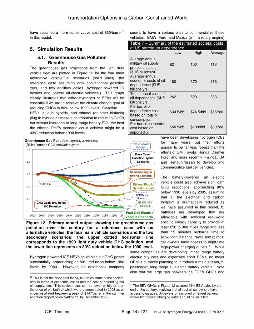
The greenhouse gas projections from the light duty vehicle fleet are plotted in Figure 12 for the four main alternative vehicle/fuel scenarios (solid lines), the reference case assuming only conventional gasoline cars, and two ancillary cases (hydrogen-powered IC hybrids and battery all-electric vehicles.) This graph clearly illustrates that either hydrogen or BEVs will be essential if we are to achieve the climate change goal of reducing GHGs to 80% below 1990 levels. Gasoline HEVs, plug-in hybrids, and ethanol (or other biofuels) plug-in hybrids all make a contribution to reducing GHGs, but without hydrogen or long-range battery EVs, the best the ethanol PHEV scenario could achieve might be a 43% reduction below 1990 levels.

Hydrogen-powered ICE HEVs could also cut GHG gases substantially, approaching an 80% reduction below 1990 levels by 2080. However, no automobile company

12 This is not the price paid for oil, but an estimate of the societal cost in terms of economic losses and the cost of defending our oil supply, etc. This societal cost can be lower or higher than the price of oil, both of which were demonstrated in 2008 as oil prices oscillated between a peak of $147/barrel in the summer and then dipped below $40/barrel by December 2008.

seems to have a serious plan to commercialize these vehicles. BMW, Ford, and Mazda (with a rotary engine)

have been developing hydrogen ICEs for many years, but their efforts appear to be far less robust than the efforts of GM, Toyota, Honda, Daimler, Ford, and more recently Hyundai/KIA and Renault/Nissan to develop and commercialize fuel cell vehicles. The battery-powered all electric vehicle could also achieve significant GHG reductions, approaching 80% below 1990 levels by 2085, assuming that a) the electrical grid carbon footprint is dramatically reduced as we have assumed in this model, b) batteries are developed that are affordable with sufficient real-world specific energy capacity to provide at least 250 to 300 miles range and less than 15 minutes recharge time to allow long distance travel, and c) most car owners have access to night-time high-power charging outlets13. While

some companies are developing limited range battery electric city cars and expensive sport BEVs, no major OEM is currently planning to introduce a main stream, 5-passenger, long-range all-electric battery vehicle. Note also that the large gap between the FCEV GHGs and

13 The BEV GHGs in Figure 12 assume 98% BEV sales by the end of the century, implying that almost all car owners have access to garages, driveways or assigned off-street parking where high-power charging outlets could be installed.

Table 7 – Summary of the estimated societal costs of US petroleum dependence Low High Average

Average annual military oil supply protection costs ($US billions/yr)

82 153 118

Average annual economic costs of oil dependence ($US billions/yr)

160 370 265

Total annual costs of oil dependence ($US billions/yr)

242 523 383

Per barrel oil dependence cost based on total oil consumption

$34.5/bbl $74.5/bbl $55/bbl

Per barrel economic cost based on imported oil

$50.5/bbl $109/bbl $80/bbl

-

0.5

1.0

1.5

2.0

2.5

2000 2010 2020 2030 2040 2050 2060 2070 2080 2090 2100

Greenhouse Gas Pollution (Light duty vehicles only)

(Billion/ tonnes CO2-equivalent/year)

1990 GHG

GHG Goal: 80% below

1990 Pollution

Fuel Cell Electric

Vehicle Scenario

Ethanol Plug-In

Hybrid Scenario

Gasoline Plug-In

Hybrid Scenario

PHEVs

Base Case:

Gasoline Hybrid

Scenario

100% GasolineVehicles

Battery EVScenario

H2 ICE HEV Scenario

Figure 12 Primary model output showing the greenhouse gas pollution over the century for a reference case with no alternative vehicles, the four main vehicle scenarios and the two secondary scenarios; the upper dotted horizontal line corresponds to the 1990 light duty vehicle GHG pollution, and the lower line represents an 80% reduction below the 1990 level.



the BEV GHGs in the 2030 to 2050 time period. The BEV is penalized in the first half of the century by the existing electrical grid, dominated in most parts of the country by burning coal. The costs and time to replace these plants or to add CCS will be large. Hydrogen, on the other hand, will start off with a 50% GHG reduction from the first FCEV sold, since hydrogen made from natural gas cuts GHGs in half compared to burning gasoline in ICVs. Some individuals and organizations are promoting other fossil fuels such as diesel or natural gas to marginally reduce GHGs compared to using gasoline in HEVs or PHEVs. We have therefore included both diesel and natural gas HEVs and PHEVs in the simulation. The resulting GHGs for these transitional fossil fuels are summarized in Figure 13, which shows GHG results for all the options in 2050 and again in 2100. In all cases, diesel fuel reduces GHGs slightly relative to gasoline and natural gas cuts GHGs compared to diesel in each class of alternative vehicle. Neither of these fossil fuels could achieve even 40% reduction in GHGs below 1990 levels.

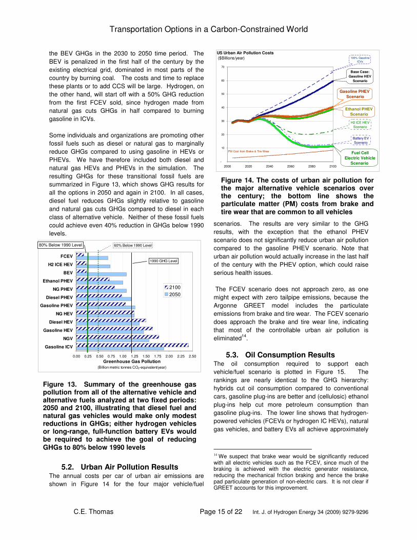
5.2. Urban Air Pollution Results

The annual costs per car of urban air emissions are shown in Figure 14 for the four major vehicle/fuel

scenarios. The results are very similar to the GHG results, with the exception that the ethanol PHEV scenario does not significantly reduce urban air pollution compared to the gasoline PHEV scenario. Note that urban air pollution would actually increase in the last half of the century with the PHEV option, which could raise serious health issues. The FCEV scenario does not approach zero, as one might expect with zero tailpipe emissions, because the Argonne GREET model includes the particulate emissions from brake and tire wear. The FCEV scenario does approach the brake and tire wear line, indicating that most of the controllable urban air pollution is eliminated14.

5.3. Oil Consumption Results The oil consumption required to support each vehicle/fuel scenario is plotted in Figure 15. The rankings are nearly identical to the GHG hierarchy: hybrids cut oil consumption compared to conventional cars, gasoline plug-ins are better and (cellulosic) ethanol plug-ins help cut more petroleum consumption than gasoline plug-ins. The lower line shows that hydrogen-powered vehicles (FCEVs or hydrogen IC HEVs), natural gas vehicles, and battery EVs all achieve approximately

14 We suspect that brake wear would be significantly reduced with all electric vehicles such as the FCEV, since much of the braking is achieved with the electric generator resistance, reducing the mechanical friction braking and hence the brake pad particulate generation of non-electric cars. It is not clear if GREET accounts for this improvement.

0.00 0.25 0.50 0.75 1.00 1.25 1.50 1.75 2.00 2.25 2.50

Gasoline ICV

NGV

Gasoline HEV

Diesel HEV

NG HEV

Gasoline PHEV

Diesel PHEV

NG PHEV

Ethanol PHEV

BEV

H2 ICE HEV

FCEV

21002050

Greenhouse Gas Pollution

(Billion metric tonnes CO2-equivalent/year)

60% Below 1990 Level80% Below 1990 Level

1990 GHG Level

Figure 13. Summary of the greenhouse gas pollution from all of the alternative vehicle and alternative fuels analyzed at two fixed periods: 2050 and 2100, illustrating that diesel fuel and natural gas vehicles would make only modest reductions in GHGs; either hydrogen vehicles or long-range, full-function battery EVs would be required to achieve the goal of reducing GHGs to 80% below 1990 levels

-

10

20

30

40

50

60

70

2000 2020 2040 2060 2080 2100

Fuel Cell

Electric Vehicle

Scenario

Ethanol PHEV

Scenario

Gasoline PHEV

Scenario

Base Case:

Gasoline HEV

Scenario

100% GasolineICVs

US Urban Air Pollution Costs

($Billions/year)

H2 ICE HEVScenario

Battery EVScenario

PM Cost from Brake & Tire Wear

Figure 14. The costs of urban air pollution for the major alternative vehicle scenarios over the century; the bottom line shows the particulate matter (PM) costs from brake and tire wear that are common to all vehicles



the same reductions in oil use, dipping very close to zero by the 2080 time period.

Two reference horizontal lines are also shown in Figure 15, corresponding to degrees of improved energy security. For decades politicians have espoused the goal of “energy independence,” which implies the total elimination of imported fossil fuels. But producing all of our own petroleum is not achievable in the foreseeable future and would not even be economically desirable. Producing oil in Saudi Arabia and shipping it here is less costly than producing oil in the US, especially after we passed our peak oil production point in 1971. So in normal times, the US economy would suffer if we produced all our own oil, even if that were physically feasible. Furthermore, given our shrinking petroleum resources, one could argue that it would be prudent in peacetime to minimize domestic oil production to save our domestic reserves for future crises and future generations. The faster we drill, the faster we deplete our finite petroleum reserves. But oil is no ordinary commodity. With 98% of our transportation needs and many other products from plastics to chemicals currently dependent on petroleum, our national security would be substantially enhanced if we set and achieve reasonable goals to significantly reduce oil consumption. Eliminating all imports is neither realistic nor necessary [32]. We imported more oil from Canada (18.8%) than Saudi Arabia (12.3%) in 2007 [33]. We imported 63% more oil from Canada and Mexico

combined (29.2%) than from all Persian Gulf countries (17.9%). The 13 OPEC countries provided 49% of all US imports in 2007, so 51% came from other nations. One goal might therefore be to cut US oil imports to 51% of current levels, so that non-OPEC nations could potentially supply most of our import needs in a crisis15, minimizing the chances of an OPEC-like organization using embargo threats to achieve political purposes. This goal assumes that the 39 non-OPEC countries that currently supply some oil or petroleum products to the US could sustain their current export levels to the US in the coming decades in spite of their own declining fossil fuel resources. A second more stringent goal might be to limit our imports to the American hemisphere. To quantify these two import restriction goals, we assume that all oil used in industry, commercial, residential, and all transportation except for light duty vehicles remains at 2007 levels, as shown in Table 8. In other words, we assume that all oil reductions are made in the light duty vehicle fleet, and all other sectors keep their consumption level fixed in the future. If industry Table 8 – Derivation of two oil reduction goals (2007 billion barrels/year) Total US consumption 7.57

Light-Duty Vehicle consumption

3.23

Non-LDV consumption 4.34

Americas

Only

US + non-OPEC imports

US Production 3.01 3.01

Americas imports (North, South & Caribbean)

1.84

All non-OPEC imports 2.72

Total oil available 4.86 5.73

Total available for light-duty vehicle use

0.52 1.40

produces more plastic from petroleum, for example, then they would have to do so more efficiently or use non-petroleum substitutes to keep oil consumption constant. As shown in Table 8, for the Americas-only case, we assume that all North American, South American, and Caribbean countries maintain their current imports to the US, and US domestic oil consumption remains flat.

15 Some nations supplying oil to the US also depend on OPEC and particularly the Persian Gulf states. Canada, for example, supplies the US with 18.8% of our imports, or approximately 2.3 million barrels/day. But Canada also imports approximately 1.2 million gallons to its eastern provinces, including 0.44 million gallons/day from the Persian Gulf. So even if we achieve the more stringent of these two goals, the global economy would still have significant dependence on OPEC oil.

-

1.0

2.0

3.0

4.0

5.0

6.0

2000 2020 2040 2060 2080 2100

Oil Consumption

(Billion barrels/year)

FCEV, H2 ICE

HEV & BEV

Scenarios

Gasoline PHEV

Scenario

PHEVs

Ethanol PHEV

Scenario

Base Case:

Gasoline HEV

Scenario

100% GasolineVehicles

Non-OPEC-only Oil

American-only Oil

Figure 15. Oil consumption for the major alternative vehicle scenarios over the century; the upper horizontal dashed line indicates the oil consumption level that might be accommodated by non-OPEC nations, and the lower dashed line indicates the oil consumption level that might be provided in a crisis from the American continent – one representation of “energy independence”



This level of production would leave approximately 0.52 billion barrels/year (1.42 million barrels/day) of oil for the LDV market, the lower dashed line in Figure 15. Similarly, if we assume that all non-OPEC nations including our European NATO allies continue supplying oil to the US at current rates, then there would be 1.4 billion barrels/year (3.83 million barrels/day) left over for LDVs, the upper dashed line in Figure 15. We conclude that the ethanol/biofuels PHEV could achieve quasi-independence from OPEC, but the only options that could achieve the Americas-only goal would be hydrogen-powered vehicles, natural gas vehicles or battery EVs. These non-oil dependent vehicles could achieve energy quasi-independence by 2045 in terms of using oil only from non-OPEC nations and by 2055 in terms of using only oil in a crisis from the Americas. Natural gas consumption would not be sustainable, however, so some combination of hydrogen and electricity will be required to achieve oil quasi-independence.

5.4. Societal Cost Saving Results As described in Section 4.9 above, we monetized the costs of greenhouse gas emissions, urban air pollution, and imported oil for each vehicle/fuel combination, resulting in an estimated societal dollar cost for each year. The resulting total societal costs are plotted in Figure 16 for each major vehicle/fuel scenario. The savings over time are huge. The hydrogen FCEV scenario would cut societal costs by up to $480 billion per year by the end of the century compared to business-as-usual with conventional (non-hybrid) gasoline cars. Relative to gasoline hybrids, the more realistic comparison for the future, the hydrogen FCEV scenario would save society approximately $330 billion per year in reduced urban air pollution, reduced GHGs, and reduced oil consumption. The hydrogen IC HEV and the BEV scenarios would generate similar savings. The gasoline-powered PHEV scenario would save approximately $130 billion and the cellulosic ethanol PHEV scenario about $200 per year relative to the HEV scenario by the end of the century. 6. Sensitivity Analyses These simulation results, like all models, depend on the input assumptions. We have analyzed the sensitivity of the main results to several key input assumptions including:

• Alternative vehicle fuel economy • Degree of carbon footprint reduction for

hydrogen and electricity

• Fuel cell vehicle market entry date • Fraction of PHEVs with access to charging ports • Amount of cellulosic ethanol production 6.1. Sensitivity to Fuel Economy

Assumptions We varied the relative fuel economy values from the minimum to the maximum estimates cited in the

-

100

200

300

400

500

600

2000 2020 2040 2060 2080 2100

Total Societal Costs ($Billion/year)

Fuel Cell Electric

Vehicle Scenario

Ethanol Plug-in

Hybrid Scenario

Gasoline Plug-in

Hybrid Scenario

PHEVs

Base Case:

Gasoline Hybrid

Scenario

100% GasolineICEVs

Battery ElectricVehicle Scenario

Figure 16. Estimate of the total societal costs of greenhouse gas pollution, urban air pollution and the economic and military costs of imported oil for the major alternative vehicle scenarios (the hydrogen-powered ICE HEV scenario has approximately the same societal costs as the FCEV scenario)

0.0

0.2

0.4

0.6

0.8

1.0

1.2

1.4

1.6

1.8

2.0

1 1.5 2 2.5 3

Greenhouse Gas Pollution in 2100 (Light duty vehicles only)


Fuel Economy Relative to Gasoline ICV

Base Case:

Gasoline Hybrid

Scenario

Gasoline Plug-in

Hybrid Scenario

Ethanol Plug-in

Hybrid Scenario

H2 ICE HEVScenario

Fuel Cell Electric

Vehicle Scenario

Figure 17. Sensitivity of greenhouse gas pollution in 2100 to the alternative vehicle fuel economy relative to a gasoline ICV; the triangles below each line indicate the fuel economy assumed for that vehicle type in the base case (the year 2100 was chosen to show maximum impact of the fuel economy assumptions)



literature for each of the alternative vehicle options. To best illustrate the impact of fuel economy on greenhouse gases, we plotted the GHGs in the year 2100 when the alternative vehicles have maximum impact on the outcome. As shown in Figure 17, GHGs from hybrid electric vehicles decrease with increasing estimated fuel economy, but the relative relationships between vehicles remain unchanged from the base case. In particular, the fuel cell electric vehicle scenario remains the best option to cut GHGs, and hydrogen-powered cars would be required to achieve the 80% GHG reduction goal. The plots for urban air pollution, oil consumption, and total societal costs are similar to the GHG graph and are not shown here.

6.2. Sensitivity to carbon footprint The model assumes that the carbon emissions from hydrogen and electricity production decrease over time, approaching zero by 2100. To simulate the effects of less carbon footprint reduction, we increased the fraction of electricity and hydrogen made from natural gas in 2100 as shown in Figure 18. The low-carbon scenarios (FCEV, BEV, and H2 ICE HEV) are most affected by increasing natural gas content, but the relative rankings of the scenarios remain unchanged up to 30% natural gas feedstock for both electricity and hydrogen16. .

16 Utilizing this much natural gas will probably not be economically feasible by the end of the century, given the world’s current use of this non-renewable resource; this chart is meant only to illustrate the impact of increased carbon content on GHGs from hydrogen and electricity production.

6.3. Sensitivity to FCEV market launch date

Another key input to this model is the time period when FCEVs will be affordable and when hydrogen infrastructure can be installed to support a growing fleet of FCEVs. We assume that major sales begin in the 2015 time period, with more than 44,000 FCEVs sold or leased in the US by 2015, rising to more than 765,000 by 2020. Delaying FCEV market entry does not substantially affect the relative relationships between the FCEV and the other vehicles with respect to GHGs, urban air pollution or gasoline consumption---all FCEV scenario curves are simply shifted to the right. The greatest impact of delaying market entry is the added societal costs by foregoing the savings resulting from FCEVs. Initially, each year of FCEV delay causes over $300 billion of cumulative lost societal savings over the century. Figure 19 shows the annual and cumulative lost savings for a 10-year delay in FCEV market entry. By mid-century the annual societal costs would grow to $70 billion per year, tapering off as FCEVs reached market saturation by the last half of the century. As early as 2020 the national costs for GHGs, urban air pollution, and oil imports would be $2.5 billion larger with a 10-year delay in FCEV market entry. These cumulative societal lost savings would exceed $16 billion by 2025, which could be sufficient to fund the initial hydrogen infrastructure system. The total cumulative lost savings of delaying FCEVs by ten years would be almost $3 trillion dollars over the century.

0.0

0.2

0.4

0.6

0.8

1.0

1.2

1.4

1.6

1.8

0% 5% 10% 15% 20% 25% 30% 35% 40%



Natural Gas Fraction in 2100(for both hydrogen and electricity production)

H2 ICE HEVScenario

BEVScenario

Base Case

Base Case:

Gasoline Hybrid

Scenario

Gasoline Plug-in

Hybrid Scenario

Ethanol Plug-in

Hybrid Scenario

Fuel Cell Electric

Vehicle Scenario

Figure 18. Sensitivity of greenhouse gas pollution in 2100 to the fraction of natural gas used to make hydrogen and to make electricity (natural gas is used as a surrogate for increased carbon footprint for each fuel)

-

10

20

30

40

50

60

70

80

2000 2010 2020 2030 2040 2050 2060 2070 2080 2090 2100

$-

$500

$1,000

$1,500

$2,000

$2,500

$3,000

$3,500

Annual Societal Cost of

10-Year FCEV Delay

($Billion/year)

Annual Societal Cost of

10-Year FCEV Delay

Cumulative Costs of

10-Year FCEV Delay

Cumulative Societal Cost

of 10-Year FCEV Delay

($Billion)

Figure 19. Estimated annual societal cost of delaying the introduction of fuel cell electric vehicles by ten years (left curve & left axis), and the cumulative societal cost of such a delay (right curve and right axis)



6.4. Sensitivity to PHEV charging access fraction

The base case PHEV scenarios (gasoline and ethanol) assume that up to 75% of all light duty vehicle owners would have access to and would consistently use a night-time charging outlet. This was intended to cover car owners with garages, car ports, driveways or assigned off-street parking at apartment complexes that could accommodate an outside electrical power outlet. Figure 20 summarizes the impacts of 2100 market share on GHGs for all major vehicle options, showing that the relative GHG emissions rankings would not change even if the PHEVs increased their market share from 75% to 100% and the FCEV, HEV, and BEV market shares were decreased from the assumed 98% market share in 2100 down to 75%. However, the battery EV scenario could not quite reach the 80% reduction in GHGs from 1990 levels if BEVs were limited to 75% of all vehicles as a result of limited night-time charging outlets17.

17 Limitations on BEV charging outlets should probably be more stringent than for PHEVs, since BEVs will require much higher power circuits than PHEVs. One could make the case that BEVs should have lower market penetration than PHEVs. We have, however, kept the BEV market share at 98%, equal to the FCEV, to make direct comparisons between these two options.

6.5. Sensitivity to Cellulosic Ethanol Production

The ethanol PHEV scenario assumes a maximum sustainable US production capacity of 140 billion gallons per year, although the NRC has estimated that a ceiling of 45 billion gallons per year may be more realistic as discussed in Section 4.8. The impact of ethanol production on GHG emissions in 2100 between these extremes of 45 billion and 140 billion gallons/year is also shown in Figure 20. At 45 billion gallons/year, there would not be enough ethanol to support 50% PHEV market penetration, as shown by the flat line in Figure 20. At 90 billion gallons/year, GHGs would decrease until approximately 80% PHEV market share. But even if agribusinesses could achieve production volumes of 140 billion gallons per year, plug-in hybrids using biofuels could not achieve an 80% reduction in greenhouse gases anytime in this century.

7. Conclusions The major conclusions from these computer simulations are: Greenhouse gas reductions: the hydrogen-powered fuel cell electric vehicle, in conjunction with hybrids, plug-in hybrids, and biofuels, is the best option to achieve the goal of reducing GHGs by 80% or more below 1990 levels in the transportation sector, although not until 2067 with the parameters in this model; the second-best option, the hydrogen-powered ICE hybrid electric vehicle, could achieve this goal by 2080; and the battery-powered electric vehicle, if accepted by a

large fraction of drivers as a full-function, long-

range passenger vehicle18 , by 2085. Cellulosic

18 In a previous publication, we showed that a long-range battery electric vehicle would be inferior to a fuel cell electric vehicle in terms of weight, onboard storage volume, mass production cost, life-cycle cost, fueling time, and would require more natural gas or biomass to travel a given distance; the BEV

0.0

0.2

0.4

0.6

0.8

1.0

1.2

1.4

1.6

1.8

2.0

50% 60% 70% 80% 90% 100%



Market Share in 2100

Base Case:

Gasoline HEV

Scenario

Ethanol PHEV

Scenarios

Fuel Cell Electric

Vehicle Scenario

GHG Goal: 80% below 1990 level

45 B gal/yr

90 B gal/yr

140 B gal/yr

Gasoline PHEV

Scenario

BPEV Scenario

Figure 20. Sensitivity of greenhouse gas pollution to the assumed maximum market shares by 2100 for the alternative vehicle scenarios, including the impact of limiting cellulosic ethanol production to 60, 90 and 140 billion gallons per year; the triangles below each set of lines corresponds to the assumed market share in each scenario (75% for all PHEVs and 98% for all others)



ethanol 19 plug-in hybrids could at best reduce GHGs by 50% by the end of the century, while gasoline-powered plug-in hybrids by themselves could only reduce GHGs to 20% below 1990 levels by the end of the century. Petroleum consumption: hydrogen-powered vehicles (fuel cell or hydrogen ICE hybrids), natural gas vehicles, and all-electric battery vehicles are the only options that could achieve energy “quasi-independence20

,” reaching that milestone by mid-century; the second-best option, ethanol PHEVs would still consume over three times the current petroleum capacity of the American continent by the end of the century.

Urban air pollution: the hydrogen-powered fuel cell electric vehicle and the battery-electric vehicle are the only options that would eliminate nearly all controllable 21 urban air pollution from the transportation sector by 2100; all other vehicle/fuel options including both gasoline and biofuel PHEVs would produce essentially the same or greater urban air pollution as the existing car fleet due to increased vehicle miles traveled over the century. Societal cost savings: hydrogen-powered vehicles (fuel cell or hydrogen ICE hybrids) and full-function battery electric vehicles, if acceptable to a large

fraction of drivers, would provide greater societal cost savings than either gasoline or biofuel plug-in hybrids. The hydrogen-powered vehicle and full-function battery electric vehicle scenarios would reduce societal costs by up to $330 billion per year by the end of the century compared to the gasoline hybrid electric vehicle scenario. Plug-in hybrid electric vehicles alone would produce lower societal costs saving: approximately $200 billion savings per year for the (cellulosic) ethanol plug-in hybrid scenario and $130 billion per year savings for the gasoline plug-in hybrid scenario.

would have lower fuel cost per kilometer and would require less renewable electricity per mile than the FCEV [34]. 19 Existing corn-based ethanol could not even reach this level of GHG reduction. 20 “Quasi-independence” is defined here as reducing oil consumption in the transportation sector to the level that US domestic oil production plus imports from the Americas (North, Central, South, and Caribbean) could supply all petroleum needs in a crisis, assuming no growth in non-transport oil consumption and no further decline in American oil production capacity. 21 Particulate emissions from brake & tire wear continue for all vehicles.

Costs of delaying the introduction of hydrogen vehicles. The cumulative societal costs over the century for each year of delay in the introduction of hydrogen-powered fuel cell electric vehicles amounts to approximately $300 billion. If hydrogen-powered vehicle market entry is delayed from 2015 to 2025, for example, cumulative societal costs would increase by $16 billion in 2025, which would most likely be sufficient to pay for the initial hydrogen infrastructure. Total cumulative costs over the century of this ten-year delay would be $3 trillion.

We conclude that society will require a full portfolio of alterative vehicle and fuel options to achieve our environmental and energy security objectives. No single alternative such as biofuels, a plug-in hybrid or a long-range battery electric vehicle will alone reach our objectives. Given the technical and economic uncertainties of sustainable biofuel production and both fuel cells and high energy batteries for PHEVs, and particularly for long-range BEVs, governments should vigorously and consistently fund all three options until one or more can meet our needs and survive in the marketplace without subsidies. The triple threats of global warming, energy security, and urban air pollution are too great to rely on any one transportation option for the foreseeable future.

Acknowledgments

This author would like to thank Joan Ogden (then at Princeton) for her pioneering work first reported in 1989 that introduced this author to the renewable hydrogen field [35]. We would also like to thank the many people who have contributed over the years to the development and review of these vehicle simulation models, beginning with Ira Kuhn, Brian James, George Baum, Julie Perez, and their colleagues at Directed Technologies, Inc.; Ron Sims, Brad Bates, Mujeeb Ijaz, and colleagues (then at the Ford Motor Company); Bob Shaw (Arête); Barney Rush (CEO), Frank Lomax (CTO), and all our co-workers at H2Gen Innovations, Inc.; the financial support of the Department of Energy over many years and the contributions from DOE staff including, among others, Sig Gronich, Neil Rossmeissl, Steve Chalk, JoAnn Milliken, Pat Davis, Mark Paster, Fred Joseck, Tien Nguyen, Arlene Anderson, Rick Farmer,



and Sunita Satyapal; Joan Ogden, Mark Delucchi, and their colleagues at the University of California at Davis; Michael Wang, Amgad Elgowainy, and colleagues at the Argonne National Laboratory; George Sverdrup and Marc Melaina at the National Renewable Energy Laboratory; Bob Rose at the US Fuel Cell Council; and the National Hydrogen Association task force that developed a new hydrogen energy story, the “Energy Evolution”, headed by Frank Novachek of Xcel Energy with representatives from the automobile and energy industries, academia, and the national laboratories. And a final thanks to the reviewers of this article for their helpful suggestions and changes. References 1. Davis SC, Diegel SW, Boundy RG. Transportation

Energy Data Book, 27th Edition, Center for Transportation Analysis, Oak Ridge National Laboratory #6981, US Department of Energy, 2007.

2. Ruselowski G, Wallace JP, Choudhury R, Wang M, Weber T, Finizza A. Well-to-wheels energy use and greenhouse gas emissions of advanced fuel/vehicle systems—North American analysis, Vol 1, General Motors, the Argonne National Laboratory, BP, ExxonMobil, and Shell, June 2001

3. Brinkman N, Wang M, Weber T, Darlington T. Well-to-wheels analysis of advanced fuel/vehicle systems—A North American study of energy use, greenhouse gas emissions, and criteria pollutant emissions, General Motors and the Argonne National Laboratory, May 2005

4. Edwards R, Larivé J-F, Mahieu V, Rouveirolles P. Well-to-wheels analysis of future automotive fuels and powertrains in the European context, Concawe/ EUCAR / European Commission Version 2c, March 2007

5. Kromer MA, Heywood JB. Electric powertrains: opportunities and challenges in the U.S. light-duty vehicle fleet, Sloan Automotive Laboratory Report # LFEE 2007-03 RP, Massachusetts Institute of Technology, May 2007 http://web.mit.edu/sloan-auto-lab/research/beforeh2/files/kromer_electric_powertrains.pdf (Accessed September 2009)

6. Kromer MA, Heywood JB. A comparative assessment of electric propulsion systems in the 2030 US light-duty vehicle fleet. Society of Automotive Engineers: Warrendale, Pennsylvania, Technical Paper Series 2008-01-0459, April 2008.

7. Electric Power Research Institute and the Natural Resources Defense Council. Environmental Assessment of Plug-In Hybrid Electric Vehicles;

Volume 1: Nationwide Greenhouse Gas Emissions, Final Report 1015325, July 2007.

8. National Research Council of the National Academy of Engineering. The Hydrogen Economy: Opportunities, Costs, Barriers, and R&D Needs, 2004, http://www.nap.edu/catalog/10922.html (Accessed September 2009)

9. National Research Council of the National Academies, Ramage MP, Chair. Committee on Assessment of Resource Needs for Fuel Cell and Hydrogen Technologies. Transitions to alternative transportation technologies: a focus on hydrogen, 2008. http://books.nap.edu/catalog.php?record_id=12222 (Accessed September 2009)

10. Wang MQ. Greenhouse gases, Regulated Emissions, and Energy use in Transportation (GREET), The Argonne National Laboratory, http://www.transportation.anl.gov/modeling_simulation/GREET/index.html (Accessed September 2009)

11. Thomas CE, James BD, Lomax FD, Kuhn IF. Integrated analysis of hydrogen passenger vehicle transportation pathways, National Renewable Energy Laboratory Subcontract No. AXE-6-16685-01, Directed Technologies, Inc., Arlington, Virginia, March 1998

12. Wipke K, Anton D, Spirk S. Evaluation of range estimates for Toyota FCHV-adv under open road driving conditions, National Renewable Energy Laboratory and Savannah River National Laboratory, 3 SRNS-STI-2009-00446, August 2009, http://www.nrel.gov/hydrogen/proj_learning_demo.html (Accessed September 2009)

13. Elgowainy A, Burnham A, Wang M, Molburg J, Rousseau A. Well-to-wheels energy use and greenhouse gas emissions analysis of plug-in hybrid electric vehicles, Argonne National Laboratory report ANL/ESD/09-2, February 2009 & SAE 2009-01-1309.

14. de la Chesnaye F. Analysis of the Climate Stewardship and Innovation Act of 2007, S.280, U.S. Environmental Protection Agency, Office of Atmospheric Programs, July 16, 2007, www.epa.gov/climatechange/economicanalyses.html (Accessed September 2009)

15. Energy Information Administration. Energy Market and Economic Impacts of S.280, the Climate Stewardship and Innovation Act of 2007, EIA Report # SR/OIAF/2007-04, July 2007.

16. Delucchi MA. A lifecycle emissions model (LEM): lifecycle emissions from transportation fuels, motor vehicles, transportation modes, electricity use, heating and cooking fuels, and materials, Institute for Transportation Studies, University of California,



Davis, Report # UCD-ITS-RR-03-17, December 2003, Table 15, pg. 330

17. Sandia National Laboratory and General Motors. 90-billion gallon deployment study, February 2009. http://hitectransportation.org/news/2009/Exec_Summary02-2009.pdf (Accessed September 2009)

18. Perlack RD, Wright LL, Turhollow AF, Graham RL, Stokes BJ, Erbach DC. Biomass as a feedstock for a bioenergy and bioproducts industry: the technical feasibility of a billion-ton annual supply, Oak Ridge National Laboratory Report TM-2005/66, Oak Ridge, Tennessee, April 2005

19. Greene N. Growing energy: how biofuels can help end America’s oil dependence, Natural Resources Defense Council, Washington, D.C., December 2004.

20. Kimbrell, A. The real price of gasoline: an analysis of the hidden external costs consumers pay to fuel their automobiles, International Center for Technology Assessment Report #3, Washington D.C., November 1998

21. Delucchi MA. Summary of the nonmonetary externalities of motor-vehicle use; Report #9: The Annualized Social Cost of Motor-Vehicle Use in the United States based on 1990-1991 Data, University of California at Davis, Report# UCD-ITS-RR-96-3 (9) rev.1, September 1998, Revised October 2004.

22. Litman TA. Transportation Cost Analysis: Techniques, Estimates and Implications, Victoria Transport Policy Institute, June 2002.

23. AEA Technology Environment. Damages Per Tonne Emission of PM2.5, NH3, SO2, Nox and VOCs from each EU25 Member State, Clean Air for Europe (CAFÉ) Programme, European Commission, 2005

24. Holland M, Watkins P. Estimates of Marginal External Costs of Air Pollution in Europe, European Commission, 2002

25. Wang MQ, Santini DJ, Warinner SA. Methods of Valuing Air Pollution and Estimated Monetary Values of Air Pollutants in Various US Regions, Argonne National Lab, 1994

26. Wang MQ, Santini DJ, Warinner SA. Monetary Values of Air Pollutants in Various US Regions, Transportation Research Record, 1475, pp. 33-41,1995.

27. Ogden JM, Williams RH, Larson ED. Societal lifecycle cost of cars with alternative fuels/engines. Energy Policy 32 (2004) 7-27

28. Klare MT. Blood and oil: the dangers and consequences of America’s growing dependency on imported petroleum, Owl Books, New York 2004

29. Copulos MR. America's achilles heel: the hidden cost of imported oil; a strategy for energy

independence, The National Defense Council Foundation, Washington D.C. October, 2003

30. Copulos MR. The hidden cost of oil: an update, The National Defense Council Foundation, Washington, D.C. January 8, 2007

31. Danks A, Orisich M, Smith S. The military cost of securing energy. The National Priorities Project, Northhampton, Massachusetts October 2008. www.nationalpriorities.org/auxiliary/energy_security/full_report.pdf (accessed September 2009)

32. Greene DL, Leiby PN. Oil independence: realistic goal or empty slogan? Oak Ridge National Laboratory, March 2007 http://pzl1.ed.ornl.gov/GreeneAndLeiby2007%20Oil%20Independence-Realistic%20Goal%20or%20Empty%20Slogan.html (accessed September 2009)

33. US Department of Energy, Energy Information Administration. Net Imports of Total Crude Oil and Products into the U.S. by Country , August 2008 (accessed September 2009)

34. Thomas CE. Fuel cell and battery electric vehicles compared, Int. J. of Hydrogen Energy 34 (2009) 6005-6020.

35. Ogden JM, Williams RH. Solar hydrogen: moving beyond fossil fuels, World Resources Institute, Washington D.C., October 1989.

transportation options in a carbon-constrained world: hybrids, plug-in hybrids … ·...

Documents