transportation energy futures series: vehicle technology
TRANSCRIPT

LIGHT-DUTY VEHICLES
Vehicle Technology Deployment Pathways: An Examination of Timing and Investment Constraints

TRANSPORTATION ENERGY FUTURES SERIES: Vehicle Technology Deployment Pathways:
An Examination of Timing and Investment Constraints
A Study Sponsored by
U.S. Department of Energy Office of Energy Efficiency and Renewable Energy
March 2013
Prepared by
ARGONNE NATIONAL LABORATORY Argonne, IL 60439
managed by U Chicago Argonne, LLC
for the U.S. DEPARTMENT OF ENERGY
under contract DE-AC02-06CH11357 This report was prepared as an account of work sponsored by an agency of the United States Government. Neither the United States Government nor any agency thereof, nor any of their employees, makes any warranty, expressed or implied, or assumes any legal liability or responsibility for the accuracy, completeness, or usefulness of any information, apparatus, product, or process disclosed, or represents that its use would not infringe privately owned rights. Reference herein to any specific commercial product, process, or service by trade name, trademark, manufacturer, or otherwise, does not necessarily constitute or imply its endorsement, recommendation, or favoring by the United States Government or any agency thereof. The views and opinions of authors expressed herein do not necessarily state or reflect those of the United States Government or any agency thereof.

iv
ABOUT THE TRANSPORTATION ENERGY FUTURES PROJECT
This is one of a series of reports produced as a result of the Transportation Energy Futures (TEF) project, a U.S. Department of Energy (DOE)-sponsored multi-agency project initiated to identify underexplored strategies for abating greenhouse gases and reducing petroleum dependence related to transportation. The project was designed to consolidate existing transportation energy knowledge, advance analytic capacity-building, and uncover opportunities for sound strategic action.
Transportation currently accounts for 71% of total U.S. petroleum use and 33% of the nation’s total carbon emissions. The TEF project explores how combining multiple strategies could reduce GHG emissions and petroleum use by 80%. Researchers examined four key areas – light-duty vehicles, non-light-duty vehicles, fuels, and transportation demand – in the context of the marketplace, consumer behavior, industry capabilities, technology and the energy and transportation infrastructure. The TEF reports support DOE long-term planning. The reports provide analysis to inform decisions about transportation energy research investments, as well as the role of advanced transportation energy technologies and systems in the development of new physical, strategic, and policy alternatives.
In addition to the DOE and its Office of Energy Efficiency and Renewable Energy, TEF benefitted from the collaboration of experts from the National Renewable Energy Laboratory and Argonne National Laboratory, along with steering committee members from the Environmental Protection Agency, the Department of Transportation, academic institutions and industry associations. More detail on the project, as well as the full series of reports, can be found at http://www.eere.energy.gov/analysis/transportationenergyfutures.
Contract Nos. DC-A36-08GO28308 and DE-AC02-06CH11357

v
AVAILABILITY
This report is available electronically at http://www.osti.gov/bridge Available for a processing fee to U.S. Department of Energy and its contractors, in paper form, from: U.S. Department of Energy Office of Scientific and Technical Information P.O. Box 62 Oak Ridge, TN 37831-0062 phone: 865.576.8401 fax: 865.576.5728 email: [email protected]
Available for sale to the public, in paper form, from: U.S. Department of Commerce National Technical Information Service 5285 Port Royal Road Springfield, VA 22161 phone: 800.553.6847 fax: 703.605.6900 email: [email protected] online ordering: http://www.ntis.gov/help/ordermethods.aspx
CITATION Please cite as follows:
Plotkin, S.; Stephens, T.; McManus, W. (March 2013). Vehicle Technology Deployment Pathways: An Examination of Timing and Investment Constraints. Transportation Energy Futures Report Series. Prepared for the U.S. Department of Energy by Argonne National Laboratory, Argonne, IL. DOE/GO-102013-3708. 56 pp.

vi
REPORT CONTRIBUTORS AND ROLES
Argonne National Laboratory Steve Plotkin Lead and primary author Thomas Stephens Contributing author
Oakland University School of Business Walter McManus Contributing author

vii
ACKNOWLEDGMENTS We are grateful to colleagues who reviewed portions or the entirety of this report in draft form, including:
Jeff Alson, Senior Policy Advisor, Transportation and Climate Division, Office of Transportation and Air Quality, U.S. Environmental Protection Agency John German, Senior Fellow, Technology and U.S. Policy Lead, International Council on Clean Transportation Dr. Paul Leiby, Group Leader, Energy Analysis Group, Environmental Sciences Division, Oak Ridge National Laboratory Art Rypinski, Economist, Office of the Secretary, U.S. Department of Transportation Danilo Santini, Senior Economist, Argonne National Laboratory Participants in an initial Transportation Energy Futures scoping meeting in June 2010 – representing the U.S. Department of Energy and national laboratories – assisted by formulating innovative and timely ideas to consider for the project. Steering Committee members and observers offered their thoughtful perspective on transportation analytic research needs as well as insightful comments on an initial Transportation Energy Futures work plan in a December 2010 meeting, and periodic teleconferences through the project. Many analysts and managers at the U.S. Department of Energy played important roles in sponsoring this work and providing valuable guidance. From the Office of Energy Efficiency and Renewable Energy, Sam Baldwin and Carla Frisch provided leadership in conceptualizing the project. A core team of analysts collaborated closely with the national lab team throughout implementation of the project. These included: Jacob Ward and Philip Patterson (now retired), Vehicle Technologies Office Tien Nguyen and Fred Joseck, Fuel Cell Technologies Office Zia Haq, Kristen Johnson, and Alicia Lindauer-Thompson, Bioenergy Technologies Office The national lab project management team consisted of Austin Brown, Project Lead, and Laura Vimmerstedt, Project Manager (from the National Renewable Energy Laboratory); and Tom Stephens, Argonne Lead (from Argonne National Laboratory). Data analysts, life cycle analysts, managers, contract administrators, administrative staff, and editors at both labs offered their dedication and support to this effort.


ix
TABLE OF CONTENTS List of Figures ............................................................................................................................................. x List of Tables .............................................................................................................................................. xi Acronyms ................................................................................................................................................... xii Executive Summary .................................................................................................................................... 1 1. Introduction .......................................................................................................................................... 5 2. Rates of Technology Penetration: How Quickly Can a New Vehicle Technology Permeate
the Marketplace and the Fleet? ........................................................................................................... 9 2.1. Constructing a Plausible Timeline ................................................................................................. 9 2.2. Suggested Timeline .................................................................................................................... 20
2.3. Another Way of Looking at Timing .............................................................................................. 24
3. Examining the Business Case for a Vehicle Technology Scenario .............................................. 26 3.1. Issues with Scenario Analysis ..................................................................................................... 26
3.2. Focusing on the Supply Side ...................................................................................................... 26
3.3. Two Approaches to Examining the Business Case for Scenarios .............................................. 27
3.4. Conclusions ................................................................................................................................. 48
4. Future Work ......................................................................................................................................... 49 4.1. Building a Database of Basic Vehicle Investments ..................................................................... 49
4.2. Incorporating Cash Flow and Decision Analysis into Complex Projection Models ..................... 50
4.3. Evaluating the Timing and Investment Context of Refueling Infrastructure Deployment Required for Advanced Vehicles ................................................................................................ 52
5. Conclusions ........................................................................................................................................ 53 References ................................................................................................................................................. 54

x
LIST OF FIGURES Figure ES.1. Suggested timeline for a major technology rollout ................................................................... 2 Figure 2.1. Difference between maximum growth rates in market share ................................................... 15 Figure 2.2. Penetration of technologies in the new car fleet after introduction ........................................... 17 Figure 2.3. Vehicle sales, stock, and stock vehicle miles traveled (VMT) for a new technology ................ 20 Figure 2.4. Suggested timeline for a major technology rollout .................................................................... 21 Figure 2.5. LDV fleet sales fractions in several HFCV scenarios ............................................................... 23 Figure 2.6. HyTrans vehicle technology market shares .............................................................................. 23 Figure 2.7. Scenario to achieve an 80% reduction in GHGs from the California LDV fleet ........................ 25 Figure 3.1. Simulated industry cash flow from sales of FCVs: “No Policy” case ........................................ 30 Figure 3.2. Simple decision tree showing two-stage investment ................................................................ 34 Figure 3.3. Inputting investments into the decision tree ............................................................................. 37 Figure 3.4. Inputting the cash flows into the decision tree .......................................................................... 37 Figure 3.5. Inputting the terminal values to the decision tree ..................................................................... 38 Figure 3.6. Assigning values to the decision tree ....................................................................................... 39 Figure 3.7. Decision tree for low-volume to high-volume vehicle decisions ............................................... 40 Figure 3.8. Inputting the investments into the decision tree ....................................................................... 43 Figure 3.9. Inputting the revenue cash flows into the decision tree ............................................................ 44 Figure 3.10. Inputting the terminal values to each end branch of the decision tree ................................... 45 Figure 3.11. Assigning values to each node of the tree and to the entire tree ........................................... 47

xi
LIST OF TABLES Table ES.1. Suggested Timeline for a Major Technology Rollout ................................................................ 1 Table 2.1. Estimated Time Scales (for Each Implementation Stage) for Technology Impact .................... 16 Table 2.2. Maximum Rates of Technology Penetration under Four Potential Technology Pathways....... 18 Table 2.3. Revised Maximum Technology Penetration Rates for EPA/NHTSA Assessment .................... 19 Table 3.1. Cash Flow Table for “Option to Abandon” Case ........................................................................ 36 Table 3.2. Investments Required for Production of the Low-Volume Model and the High-Volume Model,
Nominal and Present Values at a Cost of Capital of 9% ...................................................................... 41 Table 3.3. Net Cash Flows (Not Counting Investments) from the Low-Volume Model and the High-Volume
Model, Nominal and Present Values at a Cost of Capital of 9% .......................................................... 42 Table 4.1. Sample Table of Lithium Ion Capital Costs ................................................................................ 49

xii
ACRONYMS
CAFE Corporate Average Fuel Economy CO2 carbon dioxide EPA U.S. Environmental Protection Agency EV electric vehicle FCV fuel cell vehicle GHG greenhouse gas HEV hybrid electric vehicle HFCV hydrogen fuel cell vehicle HyTrans Hydrogen Transition Model ICE internal combustion engine LDV light-duty vehicle NEMS National Energy Modeling System NHTSA National Highway Traffic Safety Administration NPV net present value NRC National Research Council PHEV plug-in hybrid electric vehicle R&D research and development RRR required rate of return SI spark ignition TEF Transportation Energy Futures Study VCM vehicle choice model WACC weighted average cost of capital

1
EXECUTIVE SUMMARY
Scenarios May Need Reality Checks on Timing and Investments Analysts may develop scenarios of the deployment of new vehicle technologies for a variety of reasons, ranging from pure thought exercises for hypothesizing about the future, to careful examinations of the possible outcomes of future policies or trends in technology, to examination of the feasibility of broad goals of reducing greenhouse gases and/or oil use. To establish a scenario’s plausibility, analysts will seek to make their underlying assumptions clear and to “reality check” the story they tell about technology development and deployment in the marketplace. This report examines two aspects of “reality checking”—(1) whether the timing of the vehicle deployment envisioned by the scenarios corresponds to recognized limits to technology development and market penetration and (2) whether the investments that must be made for the scenario to unfold seem viable from the perspective of the investment community. There are some excellent examples of scenario development that have taken a considerable effort to account for timing issues—the Massachusetts Institute of Technology report On the Road in 2035 (Bandivadekar et al. 2008) is one such example. However, a review of the literature shows that many reports discussing scenario analyses do not reveal the genesis of the deployment schedule embodied by the scenarios. The literature review also reveals that the perspective of the investment community apparently was not considered or was considered by using techniques that do not take into account the role of risk in investment decisions. This result may not be surprising—conducting an investment analysis is difficult given the variety of investment actors, the uncertainty in future costs, and a scarcity of literature on the capital costs of the key building blocks of a new technology vehicle deployment. Nevertheless, a method for examining the potential attractiveness of the required capital investments to the investment community would be extremely attractive both from the perspective of improving the credibility of scenario analyses and allowing better analysis of policies designed to stimulate investment.
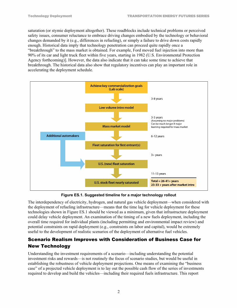
Technology Deployment Timelines Proposed This report develops a proposed timeline for introduction and penetration of a new vehicle technology, as shown in Table ES.1, which is based on Figure ES.1. The timeline indicates a period of 12 to 20+ years between the initial market introduction of a new technology and when it reaches “saturation” in the new light-duty vehicle fleet, with the lower end of the range applying primarily to technologies that do not require extensive integration into vehicle systems or substantial post-introduction cost reductions.
Table ES.1. Suggested Timeline for a Major Technology Rollout
Deployment Stage Years from Previous Stage
Achieve Key Commercialization Goals at Lab Scale
Low Volume Introductory Model 3–8 years
Mass Market Model 3–5 years
Fleet Saturation for First Entrant(s) 6–12 years
U.S. New Fleet Saturation (Additional Automakers) 3+ years
U.S. Stock Fleet Nearly Saturated 11–13 years
Total 26–41+ years, 23–33+ years after market intro
At the upper end of the timeline, the “+” indicates that, especially for more complex technologies, there are a variety of roadblocks to rapid deployment that can add substantially to the time it takes to reach
Technology Deployment TRANSPORTATION ENERGY FUTURES SERIES
2
saturation (or stymie deployment altogether). These roadblocks include technical problems or perceived safety issues, consumer reluctance to embrace driving changes embodied by the technology or behavioral changes demanded by it (e.g., differences in refueling), or simply a failure to drive down costs rapidly enough. Historical data imply that technology penetration can proceed quite rapidly once a “breakthrough” to the mass market is obtained. For example, Ford moved fuel injection into more than 90% of its car and light truck fleet within five years, starting in 1982 (U.S. Environmental Protection Agency forthcoming)]. However, the data also indicate that it can take some time to achieve that breakthrough. The historical data also show that regulatory incentives can play an important role in accelerating the deployment schedule.
Figure ES.1. Suggested timeline for a major technology rollout
The interdependency of electricity, hydrogen, and natural gas vehicle deployment—when considered with the deployment of refueling infrastructure—means that the time lag for vehicle deployment for these technologies shown in Figure ES.1 should be viewed as a minimum, given that infrastructure deployment could delay vehicle deployment. An examination of the timing of a new fuels deployment, including the overall time required for individual plants (including permitting and environmental impact review) and potential constraints on rapid deployment (e.g., constraints on labor and capital), would be extremely useful to the development of realistic scenarios of the deployment of alternative fuel vehicles.
Scenario Realism Improves with Consideration of Business Case for New Technology Understanding the investment requirements of a scenario—including understanding the potential investment risks and rewards—is not routinely the focus of scenario studies, but would be useful in establishing the robustness of vehicle deployment projections. One means of examining the “business case” of a projected vehicle deployment is to lay out the possible cash flow of the series of investments required to develop and build the vehicles—including their required fuels infrastructure. This report

TRANSPORTATION ENERGY FUTURES SERIES Technology Deployment
3
recommends that such an analysis be structured as a decision tree analysis, a method that focuses attention on the alternative decisions available to investors and the potential consequences of these decisions. Section 3 discusses this method and provides two simple examples. The method requires the analyst to develop estimates of the capital costs, projected variable costs and potential revenues of key investments, and their timing. The method also requires analysts to estimate the probability of alternative outcomes: the real possibility of investment failure for new technologies demands that analysts look beyond “best or most likely cases” and “historic industry rates of return” to get a sense for whether a scenario demanding large investments and long lead times makes sense from a business perspective. It is hoped that applying this discipline to scenario analysis will focus attention on key decisions demanded by the scenario, aid assessment of the realism of scenario goals, target risk management and risk reduction needs, and highlight the value to investors of their options—including the option to abandon the investment if markets do not develop as expected. The information provided here is not sufficient to allow the straightforward addition of cash flow and decision tree analysis to the scenario analyst’s toolbox. Future work that would help accomplish this addition includes:
• Development of a library of capital costs for the key “building blocks” of vehicle deployment (e.g., battery manufacturing facilities, assembly lines, etc.). Investment of capital requirements will have to incorporate estimates of sunk capital in conventional vehicle manufacture that must be abandoned, as well as capital requirements foregone.
• Evaluation of the timing and investment requirements for deploying alternative fuels. A great deal of the required work on capital investments is available (e.g., the extensive cost analyses of hydrogen infrastructure completed by the U.S. Department of Energy’s Hydrogen Program and the associated national laboratories and university researchers, titled “H2A”), although organizing it to be more accessible to analysts will be useful. Issues of timing, especially the constraints on rapid development, may be an especially fruitful area of further investigation.
Careful attention to timing and investment needs can improve and expedite development of robust scenarios of the rollout and market penetration of new vehicle technologies.


Technology Deployment TRANSPORTATION ENERGY FUTURES SERIES
5
1. INTRODUCTION
Reports on reducing oil use and greenhouse gas (GHG) emissions from the U.S. transportation sector generally rely on developing and analyzing scenarios of future changes in vehicles, fuels, and driving habits that offer one or more alternative pathways to achieving stringent reduction goals. Scenarios perform one or more of several functions by:
1. Assisting thinking and hypothesis development about the consequences of particular trends, events, or actions.
2. Identifying the range of possibilities of trends and policies. 3. Assessing the possibility of meeting long-term goals by evaluating what goal achievement would
require. 4. Developing a shared understanding of a problem or system across a community of stakeholders. 5. Persuasive communication of a vision for the future (adapted from Craig et al. 2002).
This report, which is part of a Transportation Energy Futures Study sponsored by the U.S. Department of Energy, identifies challenges that scenario analysts have faced and then develops some conceptual solutions to those challenges. These scenarios, which are essentially stories of the future, allow the exploration of the outcome of transportation policies or the identification of future problems by projecting key variables in expected or possible futures: world oil prices, intensity of travel, improvements in technology performance and cost, and so forth. Some scenarios are normative, i.e., they show a path required to satisfy a goal, such as a requirement for deep reductions in GHG by a certain date. Depending on the type of analysis being considered, the variables projected in the scenarios may range from basic “building block”-type variables (such as world oil prices and rates of national economic growth) to variables that reflect the outcome of expected policies and trends (e.g., vehicle miles traveled in personal vehicles or the average fuel economy of conventional vehicles at some future date). The extent to which a scenario analysis can be deemed credible and robust will lie in the extent to which its underlying assumptions and its postulated technology development seem realistic and follow some basic rules. For example, the process of moving a technology from laboratory to mass market sales requires a number of intermediate steps that can be time consuming, and so postulating an extremely rapid market penetration of a complex new technology may not be credible. Technologies that require the use of scarce resources cannot grow to levels that outstrip those resources unless new sources of the resources are discovered or new technology designs are found that reduce resource use. And scenarios that assume that private companies take enormous financial risks without measures to reduce those risks or without equivalent potential rewards are unlikely to be judged realistic. In the case of normative scenarios that seek to satisfy a goal, the examination of scenario characteristics can serve to judge the practicality of the underlying goal. The purpose of this report is to examine ways to strengthen the development of scenarios of new vehicle technology deployment, with the goal of improving their credibility and allowing more nuanced analysis of policies designed to achieve scenario goals. In particular, the report focuses on two issues:
1. Realistic timing of technology development—consideration of the schedules for vehicle technology deployment and the lag between new vehicle deployment and subsequent penetration of the stock fleet; and
2. Making sure a business case exists—“reality checking” through examining the cash flow and returns on investment of critical business decisions underlying development scenarios.
This report focuses on scenarios of vehicle technology deployment, with emphasis on technologies in early development or that have an uncertain value proposition. However, for key vehicle technologies of interest [e.g., fuel cell vehicles (FCVs), plug-in hybrid vehicles (PHEV), and battery electric vehicles],

Technology Deployment TRANSPORTATION ENERGY FUTURES SERIES
6
vehicle deployment is intimately tied to the deployment of refueling (and recharging) infrastructure (including hydrogen production and distribution and, if needed, new electricity production) and consumer behavior change to accommodate different refueling systems and, in some cases, reduced vehicle range. Deploying a refueling infrastructure—including the deployment of biomass-derived fuels—is the focus of research elsewhere in the Transportation Energy Futures project and is not discussed here. There are additional means, not evaluated here, of “reality checking” scenarios of advanced vehicle deployment. In particular, scenario development would benefit from a thorough evaluation of the upper limits to the deployment of some key technologies. For example, the deployment of battery electric vehicles demands a recharging infrastructure. This infrastructure must be deployed either simultaneously with or in advance of vehicle deployment, creating both a timing issue as well as an investment issue. In addition, however, developing a viable charging infrastructure in urban areas presents important problems, especially if potential vehicle purchasers demand, as a precursor to purchase, a guarantee of an always-accessible charging space. This issue could create strong upper limits on urban deployment, depending on consumer requirements and physical and technical limits; suburban and rural areas face other issues that might limit deployment. An additional limit on the potential magnitude of technology deployment may be mismatches between specific technology characteristics and driving habits. For example, hybrid drivetrains yield most of their benefits in stop-and-go traffic and hilly terrain and limited benefits in highway driving, so many rural and suburban drivers may obtain insufficient benefit from hybrids to overcome their added costs. The underlying objective of this report is to identify approaches that can improve scenario analyses of transport technology and fuels penetration, especially for vehicle technologies that are “disruptive” (e.g., those that require significant changes in travel behavior or in refueling) or those that are early in development and have an uncertain value to consumers. A recent examination of multiple scenario studies of future penetration of hydrogen vehicles into the U.S. vehicle fleet (Plotkin 2007) concluded the following:
Most of the analyses reported on in the reviewed literature basically skirt the issue of the transition and look at the “end state” where hydrogen has become a primary vehicle fuel. Further, most of the analyses simply postulate a degree of hydrogen penetration rather than attempting to derive the level of penetration based on an evaluation of the factors that might drive hydrogen into the LDV [light-duty vehicle] fuels market. In some cases, stock models are used to develop estimated levels of hydrogen penetration, but these depend on assumptions about sales of new hydrogen vehicles. Finally, most of the analyses do not describe any attempt to conduct a “reality check” on the scenarios, e.g. to test whether the assumed rates of development would strain industry resources or whether key investment “actors” are likely to be able to satisfy standard investment goals. 1 Thus, these analyses offer little insight about what conditions and/or policies would actually lead to their postulated levels of hydrogen penetration.
A follow-up examination of the broader transportation futures scenario literature (e.g., Plotkin and Singh, 2009; NRC, 2008; Greene et al., 2007; Yang et al., 2011; International Energy Agency, 2010; Greene and Plotkin, 2011) conducted for this study has found little change from the conditions described in Plotkin (2007). Most scenario studies appear to lack a strong foundation for projecting the technology and fuels changes described in the scenarios, although the basis for the projections vary widely, ranging from assumptions of vehicle and fuels penetration made without any apparent basis, to “normative” projections
1 Presumably, some of these analyses explicitly considered restraints on maximum growth rates, but generally these were not
documented in the literature reviewed for this study or for the 2007 report.

TRANSPORTATION ENERGY FUTURES SERIES Technology Deployment
7
that are calculated from working backwards from national goals,2 to projections based on the views of expert panels. Some projections use computer models that incorporate, at best, simple rules about industry investment in fuels and infrastructure and do not appear to take risk into account; some models estimate the penetration of new technologies by focusing only on vehicle demand, using vehicle choice models that estimate the fraction of sales captured by fuel cell and other “high technology” vehicles on the basis of their assumed characteristics and consumer valuations of these characteristics. It may not be surprising that there appears to be a weak foundation behind many of the scenario studies available to policymakers trying to make decisions about the transportation future of the United States. Projecting the future is a notoriously difficult task, and although scenarios are meant to be “possibilities,” not predictions, there are many obstacles to developing credible scenarios of U.S. transportation futures. These obstacles include: Complexity of markets. The development of new vehicle technologies—especially those requiring a new refueling infrastructure—will involve multiple actors with different risk profiles acting at different times and locations and in different places along the supply chain. The informational requirements for evaluating such markets are daunting. Volatile oil prices. The demand for transportation services and the choice of vehicles depend strongly on the price of oil; oil prices over the past several decades have been volatile, and past projections of future prices have been highly inaccurate. Uncertain technology cost and performance. The eventual long-term costs and performance of advanced transportation technologies are highly uncertain, because continued development of these technologies is likely to involve unforeseen changes in basic design and materials. Future cost reductions are often estimated by the use of “learning curves” that associate each doubling of production (or other measure of production increase) with historically established percentage reductions in costs. For a variety of reasons, particularly the bias of data underlying these curves toward “successful” technologies, the use of such curves is likely to yield overly optimistic results. Uncertain industry behavior. The willingness of vehicle manufacturers, fuel providers, and other needed industry actors to invest in new technologies and fuels is difficult to predict, especially because investment decisions may be driven by visionary thinking or by factors beyond the expected financial returns for the technology or fuel being considered (e.g., a desire to “get people into the showroom”); also, “success” demands investment by a subset of the least risk-averse investors, not investment by “average” investors, complicating the evaluation of investment prospects. In addition, some of the technologies may have multiple uses beyond just vehicle use (e.g., stationary uses for batteries), making an examination of the business case for these technologies far more complex. Uncertain consumer response. Some technologies demand that consumers change their behavior (e.g., home refueling, more careful trip planning for electric vehicles) or accept changes in performance, and thus marketplace success is less than assured. Potential for disruptions. Timetables, and even the long-term success of new technologies and fuels, can be strongly affected by unpredictable disruptions, such as accidents or rational or irrational fears and protests. International impacts. U.S. transportation technology and fuels will be strongly affected by technology and fuels developments elsewhere, especially in Europe and Asia, and these developments are hard to predict and often ignored by analysts. For example, both Japan and Europe have extensive hydrogen fuel
2 Note that scenarios based on satisfying a goal may be constructed for the purpose of deciding whether or not the goal is
realistic, not to represent a robust possible future. However, the normative scenarios examined did not appear to be constructed for this purpose (i.e., they were not “reality checked”).

Technology Deployment TRANSPORTATION ENERGY FUTURES SERIES
8
cell programs that could yield accelerated growth rates of FCVs in the United States if both the Japanese and European programs succeed and make important gains in cost reduction and performance. Note that most of these obstacles are especially relevant to technologies that are either (or both) disruptive or have not yet achieved a value proposition and are far less relevant to technologies with clear value propositions and modest need for extensive vehicle integration. The goal of this report is modest. It is not to identify ways to develop “most likely” scenarios or to gauge the relative probability of alternative scenarios. Instead, the report seeks to help analysts produce scenarios that are more transparent and consistent in their underlying assumptions and reasoning and that hopefully will become more plausible than previous scenarios. The report provides guidelines to help analysts construct scenarios that recognize constraints on the rapidity with which underlying events are likely to unfold and the conditions required to convince industries to invest in needed equipment and infrastructure. The report also seeks to identify ways to “reality check” existing scenarios to weed out those that are implausible. The ideas and procedures discussed in this report should be seen as the beginning of a needed discussion rather than as a definitive resolution of this difficult issue. Aside from further development of the basic methodology, additional work is needed to develop ways in which existing complex models can incorporate elements of the methodology. This report further suggests that analysts examine the potential cash flow of future investments, although cost estimates for the basic building blocks of vehicle deployment—battery manufacturing plants, fuel cell manufacturing facilities, changes to vehicle assembly lines (above and beyond normal costs of deploying new models), and so forth—are not readily available. Consequently, the report suggests that development of a database of these building blocks would be a useful tool in helping analysts to develop cash flow and decision tree analyses of future vehicle deployment decisions. Finally, the report suggests further evaluation of the timing and investment requirements of deploying alternative fuels.

TRANSPORTATION ENERGY FUTURES SERIES Technology Deployment
9
2. RATES OF TECHNOLOGY PENETRATION: HOW QUICKLY CAN A NEW VEHICLE TECHNOLOGY PERMEATE
THE MARKETPLACE AND THE FLEET?
2.1. Constructing a Plausible Timeline A crucial component of scenario building is to construct a plausible timeline for new vehicle technologies to enter and penetrate the light-duty fleet. The stages of market penetration include:
• Attainment of laboratory goals
• Market entry, often in a niche vehicle
• Transformation from niche to mainstream technology
• Continued penetration to maximum new vehicle fleet share
• Diffusion into the on-road fleet, beginning at market entry. It is important to recognize that there is no common language for defining the stages of market penetration, and different authors and studies often use different definitions. Further, there are various ways to measure market growth (e.g., annual percent increase in vehicle stock, annual percent increase in market share,3 annual change in market share,4 etc.). As a result, interpretation of proposed timetables and data must be handled with care. For technologies not yet in the fleet, estimating the point of likely market entry is inherently uncertain, although the primary uncertainty probably resides in estimating when performance and cost goals will be achieved in the laboratory. Most of the technologies in active consideration have achieved that milestone. [There are, however, early market entrants for electric vehicles (EVs) and PHEVs, e.g., Nissan Leaf and Chevrolet Volt.] Actual market entry after goal attainment can take several more years; the technology must be successfully manufactured and tested, and vehicle designers must integrate the technology into the appropriate vehicle system. Additional components of the timeline are the time it will take for a technology to become “mainstream,” i.e., available in multiple models, and the time it will then take to achieve maximum market share. There is a range of views, for example, regarding the rate at which the vehicle manufacturing industry can incorporate new technologies into their fleets. At the tail end of the timeline, gauging diffusion from the new vehicle fleet into the on-road fleet involves estimating on-road fleet share when new vehicle sales have been estimated. This task is relatively straightforward, using standard stock models, e.g., Argonne National Laboratory’s VISION model (Ward et al. 2008) or the stock models embedded in complex models, such as NEMS and MARKAL,5 although these can be bypassed by using the simple guidelines discussed below. However, the possibility of future changes in vehicle sales and retirements, e.g., due to recessions, adds uncertainty to this part of the diffusion timeline. In considering an appropriate timeline for new technologies, it is crucially important to recognize the differences between (1) incremental technologies that may be virtually transparent to the consumer and (2) disruptive new technologies that change important vehicle characteristics (e.g., refueling time and location) and will therefore require consumers to make adjustments in their expectations of how their vehicles will perform. Companies must be cautious in ramping up production of disruptive new
3 MN/MN−1 × 100, where M is percent market share, N is year. 4 MN−MN−1. 5 Generally, stock models will not take account of variations in vehicle miles traveled among different vehicles (except between
passenger cars and light trucks); diesel vehicles, for example, may be driven more than gasoline vehicles.

Technology Deployment TRANSPORTATION ENERGY FUTURES SERIES
10
technologies because success in marketing to “early” consumers (often called Innovators and Early Adopters) does not guarantee success with more mainstream consumers (Early Majority), who have different preferences. Box 1 provides a general description of the standard S-curve of technology diffusion and some important concerns with this depiction of the diffusion process. In addition, as discussed below, when technologies must achieve large cost reductions to appeal to a mass market, the timing and the extent of these reductions as production expands are quite uncertain. The timeline for introducing and disseminating new automotive technologies developed here relies heavily on historic data during the past few decades coupled with some adjustments based on recent experience. As discussed below, the U.S. Environmental Protection Agency (EPA), in defining a timeline for the future achievement of carbon dioxide (CO2) emission targets, has concluded that recent developments in simulation modeling, consolidation of engine families and vehicle platforms, and other factors allow vehicle manufacturers to increase the rapidity with which they can move new technologies into their fleets. Although there is little formal analysis of these trends, industry newsletters have begun discussing a trend to speedier design and deployment in the industry. For example, three articles in the April 23, 2012, edition of Automotive News discuss different aspects of this trend, focusing on:
• Using a single platform for multiple models
• “Commonizing” components across segments
• Using modular platforms
• Performing digital design of complex engine components, including simulation of crash stresses, interaction between parts, and so forth (Automotive News 2012).
The timeline presented in Section 2.2 reflects these trends to the extent that some of the minimum times have been reduced, but further analysis is needed to clarify the extent to which a new “paradigm” for deployment timing now exists. To an extent, new capabilities that can shorten deployment times may be counteracted by changes in consumer expectations for high quality and the rapidity with which the Internet allows reports of technology problems to be disseminated to consumers. As the effects of all of these factors become clearer, timelines for technology deployment can be further clarified. The process by which a new technology enters the new vehicle fleet, expands its market share, and eventually permeates the stock vehicle fleet encompasses multiple steps: Laboratory development to market introduction. Moving from achieving performance and cost goals in the laboratory to market introduction will take at least a few years, with the actual time highly dependent on the degree of integration with other vehicle systems that is required. Technologies that may affect safety or emissions incur additional testing requirements. In most cases, the initial introduction is made in one or at most a few models, to test market acceptance and to ensure that no unforeseen problems arise because of the diverse operating conditions and sometimes haphazard maintenance that is characteristic of the American market. This initial introduction allows the manufacturer to understand and manage risks, as significant problems can create high warranty costs and damage corporate reputations. The time required to assess the success of these introductory models is at least two to three years to allow sufficient operating time to identify problems (German 2009). The introductory model may be a luxury model (especially when the technology offers a content or performance boost, such as an automatic transmission with added speeds) rather than a mass-market model, although this can vary.6
6 For example, the first hybrids in the U.S. market, the Honda Insight and Toyota Prius, were not luxury models although neither
were they “mass-market” models.

TRANSPORTATION ENERGY FUTURES SERIES Technology Deployment
11
Box 1. Technology Diffusion for New (Non-Incremental)
Technologies The process of technology diffusion has often been depicted pictorially as a smooth curve, with the technology initially introduced to technology enthusiasts and gradually becoming appealing to increasing portions of the population. Figure B.1 shows a theoretical curve of a market transition to a new technology in terms of the different categories of consumers that adopt it at successive stages of the transition [adapted from Rogers (2003)]. The S-shaped logistic curve is also associated with Rogers, although in his model, the x-axis was not plotted in years. Although many analysts have adopted this or similar curves, there are important concerns associated with it:
• Rogers himself cautions that the backward-looking study of successful product innovations has created an inherent “pro-innovation bias” that leads those working on innovation to believe it is more commonly successful (easier) than is really the case. He argues that there is not enough study of slowly diffusing innovations (Rogers, p. 111).
• Probably the most important point on the curve is, according to Rogers, the “critical mass” or “takeoff” point near the intersection of the curve and the divider between Early Adopters and the Early Majority. Moore (2002) asserts that the transition from early adopter to early majority is a very difficult hurdle to get past and that making it is not guaranteed. Moore calls the transition between these two groups the “chasm.” If Moore is right and there is often a delay of share gain at that transition point, then the outset of diffusion curves, on average, would have lower rates of gain of market share early in the process than is estimated with Rogers’ standard “S.” Another possibility is simply failure to move from early adopters to the early majority, or failure even to reach the point where such a transition would begin.
Figure B.1. Theoretical market penetration curve [adapted from Rogers (2003)]
• A major reason for the possible “chasm” between early adopters and the early majority is the significant differences in consumer desires between the two groups. According to Moore, innovators are technology enthusiasts, early adopters are visionaries, and the early majorities are pragmatists. He argues that the innovators and early adopters do not communicate with the early majority and have fundamentally different goals for technology. The visionary early adopter expects a “radical discontinuity between the old ways and the new,” while the pragmatic early majority “want to buy a productivity improvement for existing operations” (Moore, p. 20). Given the fundamental difference in goals, pragmatists do not trust visionaries and will not use them as a reference.
0%
10%
20%
30%
40%
50%
60%
70%
80%
90%
100%
0 5 10 15 20 25
Perc
ent o
f Eve
ntua
l Sha
re
Year from Introduction
Innovators
Early Adopters
Early Majority
Late Majority
Laggards

Technology Deployment TRANSPORTATION ENERGY FUTURES SERIES
12
Box 1. Technology Diffusion (continued)
• According to Christenson (2003), disruptive technologies initially capture only a small portion of an existing market (e.g., innovators and early adopters) and underserve the typical consumer in the market (early majority and others). The product developers capture that share by offering a product with different attributes from the dominant technology, one or more of which is particularly attractive to that small segment of the market, even though some attributes are not attractive to consumers in the heart of the market. At the same time, a new market may be established outside of the existing market. With a solid anchor in a small market segment, the product improves over time, at a rate much more rapid than that of the presently dominant technology. In particular, the product developers move to reduce or eliminate those negative attributes that limit its attractiveness to the early majority and other market segments and enhance attributes attractive to those markets. Ultimately, the dominant technology is largely replaced—perhaps fully displaced and creatively destroyed—because the new technology has actually become superior to the formerly dominant technology. As Christensen puts it:
If and when they progress to the point that they can satisfy the level and nature of performance demanded in another value network, the disruptive technology can then invade it, knocking out the established technology and its established practitioners with stunning speed.
• Aside from the delay caused by the need to “cross the chasm,” the period of serving the innovators and early adopters is seldom a smooth one. Moore (p. 38) emphasizes that the early market process of product development before reaching the chasm between visionaries and pragmatists is difficult and iterative, with repeated feedback between customers and the product designers being critical. A dynamic of interaction between technology enthusiasts and the visionaries is described. To succeed, the entrepreneurial company must commit itself to “product modifications and system integration services it never intended to.”
The net result is that the early period of market penetration of a new technology—from market introduction to penetration of the “pragmatic” part of the market (e.g., early majority)—is seldom a smooth process, can suffer setbacks and outright failure, and can take considerably longer than portrayed in many examples of S-shaped market penetration curves. References
Christensen, C., 2003, The Innovator’s Dilemma, Harper Business Essentials. Moore, G.A., 2002, Crossing the Chasm, Harper Business Essentials, New York. Rogers, E.M., 2003, Diffusion of Innovations, 5th ed., Free Press, New York.

TRANSPORTATION ENERGY FUTURES SERIES Technology Deployment
13
Market introduction to sale of mainstream models and penetration throughout the new vehicle fleet. If the technology is successful in this introductory phase, the introducing automaker may then introduce the technology into additional models when they are redesigned in 4- to 5-year-minimum product cycles7 (German 2009; Murphy 2010), and other automakers may also introduce the technology into their fleets. If the technology is designed and produced by a major supplier, the process by which additional automakers introduce the technology may be accelerated. However, this process can be significantly slowed if the technology is not yet ready for the mass market, either because it is initially quite costly in comparison to the service it provides, or it demands important trade-offs in performance (e.g., increases noise, vibration, and harshness) or demands changes in consumer behavior. In this case, the technology’s expansion into additional models may be delayed or slowed, and overall sales may stay low for a number of years until costs come down and performance improves—assuming this occurs successfully. For example, the Honda Insight hybrid was introduced in the United States in 1999, and the Toyota Prius in 2000 (it was first introduced in Japan in 1997), but more than 10 years later, the sales share of hybrid vehicles in the U.S. market is less than 3%. What apparently is happening here is that, at recent incremental prices for hybrid drivetrains and current gasoline prices, hybrids appeal primarily to early adopters and possibly to a subset of drivers who drive greater-than-average annual miles in largely urban (or suburban) stop-and-go conditions where hybrids provide maximum benefits; hybrid technology may jump onto the standard S curve of vehicle penetration when it achieves a value proposition that appeals to mainstream drivers. An earlier example of technology penetration, port fuel injection, is discussed in German (2009). Port fuel injection was well known and used extensively by some manufacturers for years when stringent new emission standards accelerated its market penetration beginning around 1983, but despite its substantial benefits and low costs, it took 14 more years to reach 100% market penetration. Zoepf (2011) has explored “developmental lag times”—the time from market introduction to attainment of the maximum growth rate in market penetration—for a range of technologies, showing that these times have steadily decreased over the past few decades to reach an average of about 10 years today. He attributes this decline in lag times to changes in the consumer environment—more exposure to new products, large increases in communication—and improvements to supply-side capabilities, including increased reliance on suppliers and consequently more rapid distribution of intellectual property.8 Powertrain technologies tend to have the longest lag times, however. The growth rate with which a new technology spreads throughout the new vehicle fleet depends on market demand and engineering and capital resources. As noted above, new technology generally is added to a model when it undergoes a major redesign at about 4–5-year intervals. Limitations on capital and engineering resources, as well as the effect of frequent redesigns on unit costs, dictate that each automaker’s fleet has a redesign schedule that is staggered, so that it may take 8–10 years for most automakers to offer a new technology across their entire product line9 (starting at the time they decide to move the technology into their mainstream vehicles). There have been examples of some individual automakers moving considerably faster than this (EPA forthcoming). For example,
• General Motors moved lockup transmissions into 93% of its car fleet within 5 years (1978–1983).
• Ford and Honda moved fuel injection into more than 90% of their car and light truck fleets within 5 years (1982–1987 and 1985–1990, respectively).
• Toyota moved variable valve timing into 90% of its fleet in 5 years (1998–2003).
7 Product cycle: the time between major redesigns of a vehicle model. 8 Other possible reasons for accelerated penetration rates include industry consolidation of platforms, fewer and more modular
engine families, computer-aided design, flexible tooling, joint technical programs, and greater use of suppliers for major components.
9 This assumption should probably be reexamined in light of automakers’ attempts to streamline their product lines.

Technology Deployment TRANSPORTATION ENERGY FUTURES SERIES
14
• Honda moved multivalve engines into 99% of its fleet in 5 years (1985–1990).
• Hyundai moved six-speed automatic transmissions into 66% of its car fleet in a single year (2010–2011).
• Nissan moved continuously variable transmissions into 63% of its car fleet in one year (2006–2007).
The relevance of these rapid penetration rates to estimates of total fleet penetration rates is not clear. The time frames of the examples do not incorporate the period immediately following the first commercial introduction of the technologies, and some examples represent introduction into a limited array of models or engines. It would be useful to examine these examples in greater detail, especially to assess whether there is evidence that the pace of technology introduction is increasing, but undertaking this review was not possible under the time constraints of this project. It is also important to recognize the role that incentives play in moving a technology into the marketplace. The key regulatory incentives for vehicle technologies are safety, emission, and fuel economy standards. For efficiency technologies, the set of fuel economy [Corporate Average Fuel Economy (CAFE)] standards for 2011–2016 and 2016–2025 will serve as both economic incentives (there are fines for noncompliance10) and social incentives—most automakers do not want the stigma of failing to comply, and customers may be less enthusiastic about purchasing from a company that cannot comply. Figure 2.1 from Zoepf (2011) tracks the role of regulations in influencing the maximum growth rates for technology market share (measured as the change in percentage market share per year11); the highest rates seem to be associated with the presence of standards. The other primary economic incentives are the price of gasoline and government subsidies for “green” vehicles, such as EVs. The alignment of both regulatory and economic incentives may be necessary to create the conditions for rapid market penetration of those new technologies that require considerable adjustments of consumer expectations. In Figure 2.1, the peak annual growth rate in market penetration for LDV technologies has ranged from 1% to 24% over the past few decades. The five fastest-penetrating technologies are all safety-related technologies [dual master cylinders, driver’s and dual front airbags, front disc brakes, and side impact beams (Zoepf 2011)]. Generally, powertrain technologies achieve maximum growth rates in the middle of the scale—from 6% to 14% per year. The fastest-penetrating technology associated with fuel economy standards was front-wheel drive, at a maximum penetration rate of 8.7% per year. Other powertrain features whose penetration was spurred by fuel economy standards are multivalve cylinders (4.3% maximum growth) and variable valve timing (6.6% maximum growth). In contrast, fuel injection, spurred by air emission standards, had a maximum growth rate of 13.4% per year (Zoepf 2011, Appendix G).
10 The penalty, as adjusted for inflation by law, is $5.50 for each tenth of a mile per gallon (mpg) that a manufacturer’s average
fuel economy falls short of the standard for a given model year multiplied by the total volume of those vehicles in the affected fleet (i.e., import or domestic passenger car, or light truck), manufactured for that model year. Source: http://www.federalregister.gov/articles/2008/05/02/08-1186/average-fuel-economy-standards-passenger-cars-and-light-trucks-model-years-2011-2015#p-336.
11 Note that this measure of the growth rate in market share, the difference in percentage market share per year, or market share in year N minus market share in year N−1, is quite different from another common measure of growth rate: the change in market share during the year divided by the original market share at the beginning of the year multiplied by 100. When market shares are still small, the addition of a relatively small increment in sales can yield a large rate of increase in the latter measure, in contrast to a small increase in the former. For example, at 1% market share, a further 1% increase in share during the year yields a 1% growth rate for the first measure and a 100% rate for the second.

TRANSPORTATION ENERGY FUTURES SERIES Technology Deployment
15
Figure 2.1. Difference between maximum growth rates in market share
(change in percent market share/year) between regulated and nonregulated features
(Source: Zoepf 2011)
The powertrain technologies incorporated in this data set—front-wheel drive, fuel injection, multivalve cylinders, and variable valve timing (Zoepf 2011)—may not (with the possible exception of front-wheel drive) be representative of the more complex technologies (e.g., hybrid drivetrains, fuel cell drivetrains) generally considered as crucial to the future reduction of carbon emissions,12 and the risks associated with the market adoption of these new technologies may be greater—and require additional time for full penetration. In addition, if fuel injection—whose growth was stimulated by emission standards—is excluded, the other three powertrain technologies never exceeded 9% maximum growth rates (Zoepf 2009, Appendix G). In all, there were 16 technologies with maximum growth rates higher than 5%, but only three of them—front-wheel drive, variable valve timing, and fuel injection—appear to require significant vehicle integration.13 Table 2.1 shows projected time scales for the various stages of fleet penetration from On the Road in 2035 (Bandivadekar et al. 2008). The stage “market competitive vehicle” refers to the time it takes, starting from the base year of the study (about 2007),14 to make the technology “broadly available across a range of vehicle categories at a low enough cost premium to enable it to become mainstream rather than niche.” The stage “penetration across new vehicle production” refers to the time needed to gain a one-quarter to one-third market share of new vehicles. Judging from the recent introduction and apparent success of new gasoline direct injection turbocharged engines from multiple automakers (e.g., Ford, Hyundai, Volkswagen, Volvo, BMW), Table 2.1’s 10-year estimate for significant penetration of the new vehicle fleet for these engines appears reasonable. The estimate for gasoline hybrids seems problematic, given the failure of hybrids to achieve greater than a 3% penetration of U.S. new vehicle sales 11 years after the 12 Adoption of front-wheel drive requires extensive changes to engine intake, exhaust, transmission, drive axles, suspension, and
brakes and also requires extensive safety testing, so it is not clear that it is less complex than the advanced drivetrains. 13 The remaining technologies are either comfort and convenience features, such as satellite radio, or safety features largely
driven by regulation (e.g., dual master cylinders, front disc brakes, and side airbags). 14 In other words, the time period is not measured from market introduction (personal communication, John Heywood,
October 11, 2011). In the study, the reference vehicles were 2005 models.

Technology Deployment TRANSPORTATION ENERGY FUTURES SERIES
16
first production hybrid vehicle was introduced to the market, but arguably this slow growth may instead imply that hybrid drivetrains remain stuck in the first phase of development, that the technology is not yet “market competitive,” given the substantial cost premium demanded by most available hybrid models. Note that the estimates for “penetration across new vehicle production” (e.g., to 25 to 33% sales) are quite conservative, implying, for example, that 2025 hybrid sales are unlikely to be more than one-third of total sales. In fact, in On the Road’s “hybrid strong” scenario, hybrids achieve 25% sales share by 2025 and 50% by 2050, with PHEVs attaining an additional 20% share in 2050. In that scenario, the annual compounded sales of hybrid vehicles is 8% for cars and 11% for trucks—quite rapid compared to past powertrain technologies, especially considering the complexity of hybrid and PHEV powertrains, but probably conservative compared to other projections attempting to show what strong action can do to reduce carbon emissions from LDVs. For example, the National Research Council’s (NRC’s) 2008 report on hydrogen FCVs (HFCVs) (NRC 2008) has a “hydrogen success” scenario that demands that FCVs increase from 2 million vehicles in 2020 to 60 million in 2035—an average compounded annual increase in vehicle stock of about 25%, although the increase is somewhat less than this when measured as a percent of total stock, which increases over time.
Table 2.1. Estimated Time Scales (for Each Implementation Stage) for Technology Impact
Vehicle Technology
Implementation State
Gasoline Direct
Injection Turbocharged
High Speed Diesel with Particulate Trap, NOx Catalyst
Gasoline Engine/
Battery-Motor Hybrid
Gasoline Engine
Battery-Motor Plug-In Hybrid
Fuel Cell Hybrid with Onboard Hydrogen Storage
Market-competitive vehicle ~ 2–3 years ~ 3 years ~ 3 years ~ 8–10 years ~ 12–15 years Penetration across new vehicle production
~ 10 years ~ 15 years ~ 15 years ~ 15 years ~ 20–25 years
Major fleet penetration ~ 10 years ~ 10–15 years ~ 10–15 years ~ 15 years ~ 20 years Total time required ~ 20 years ~ 25 years ~ 25-30 years ~ 30–35 years ~ 50 years
(Source: Bandivadekar et al. 2008)
Figure 2.2 shows the penetration over time of six key technologies in the new passenger-car fleet based on data from the EPA (2009). Five of these technologies appeared to reach their maximum penetrations within about 15–25 years, although embedded within this industry-wide penetration are multiple examples of more rapid penetration within the fleet of single manufacturers, as described above. The industry-wide data appear reasonably well aligned with the values in Table 2.1 given that the technologies in Table 2.1 are considerably more complex. The overall fastest rate appears to be that for port fuel injection: according to the EPA trends report (2009, Table 13), the annual compounded rate of increase of market share from 1979 through 1994 was about 22% (4.7% market share in 1970 to 89.5% in 1994). It is important to note, however, that the rates of market penetration illustrated in Figure 2.2 have been affected by market conditions—a long period where CAFE standards were not binding (because they had not been changed in years) and a period of declining gasoline prices—that should have slowed the penetration of fuel-saving technologies. In other words, the penetration rates implied by the figure may be viewed as conservative.

TRANSPORTATION ENERGY FUTURES SERIES Technology Deployment
17
Figure 2.2. Penetration of technologies in the new car fleet after introduction (years after first significant use)
(Source: EPA 2009)
The EPA, National Highway Traffic Safety Administration (NHTSA), and California Air Resources Board have offered timelines for technology penetration for advanced spark ignition (SI), hybrid, EVs, and PHEVs, first in an Interim Joint Technical Assessment Report on new vehicle fuel economy and GHG standards in 2010 (EPA et al. 2010), prepared in cooperation with the California Air Resources Board and California Environmental Protection Agency, and then in a significantly revised version in 2011 (EPA and NHTSA 2011). These scenarios explore rapid, high market penetration for vehicle technologies. The 2010 values are shown in Table 2.2. In the table, “Path A” assumes the potential for a 40% market share for hybrid drivetrains in 2020 and 75% in 2025, as upper bounds (not as projections of actual market share). These percentages compare to an apparent maximum of about one-third of sales by 2025 on the basis of data in Table 2.1 from Bandivadekar et al. (2008). The maximum rates in the table are described as being “based on agency expert judgment with regard to a number of factors such as manufacturer production capacity, vehicle suitability, (and) technical feasibility considerations” (EPA et al. 2011). An agency analyst described EPA’s evaluation of maximum penetration rates as reflecting EPA’s confidence that the increased use of computer-aided design, flexible tooling, and programmable computer numerical controls; shorter vehicle design cycles and fewer vehicle platforms and engine families per manufacturer; higher sustained oil and gasoline prices; and competitive pressures to minimize the time necessary to bring technologies to market—as well as changes in marketplace expectations—superseded reliance on historical rates of market share growth to define these maximum penetration rates in the post-2015 timeframe (Alson 2011).

Technology Deployment TRANSPORTATION ENERGY FUTURES SERIES
18
Table 2.2. Maximum Rates of Technology Penetration under Four Potential Technology Pathways
Model Year 2020 Model Year 2025 Path A Path B Path C Path A Path B Path C Path D
Conventional SI 100% 100% 100% 100% 100% 100% 100% Advanced SI 10% 30% 40% 50% 75% 100% 0% Hybrid vehicles 40% 30% 40% 75% 50% 75% 60% Electric vehicle 4% 4% 8% 8% 8% 15% 20% Plug-in Hybrid 4% 4% 8% 8% 8% 15% 20%
Path A is intended to portray a technology path focused on hybrid electric vehicles (HEVs), with less reliance on advanced gasoline vehicles and mass reduction, relative to Paths B and C.
Path B represents an approach where advanced gasoline vehicles and mass reduction are utilized at a more moderate level, higher than in Path A but less than in Path C.
Path C represents an approach where the industry focuses most on advanced gasoline vehicles and mass reduction, and to a lesser extent on HEVs.
Path D represents an approach focused on the use of PHEV, EV, and HEV technology, and relies less on advanced gasoline vehicles and mass reduction (EPA et al. 2010).
If hybrid vehicle market share followed Path A or C, it would reach 40% share by 2020 and 75% by 2025. These values imply a maximum market share growth rate (as MT – MT−1/year) before 2020 of at least 5% and probably quite a bit higher, as it seems unlikely that the share will see a dramatic change within the next few years; in the 2020–2025 period, the maximum market share growth rate would be at least 7% per year. These rates are not unprecedented for powertrain technologies (see Figure 2.1), although hybrid drivetrains, because they are complex and not easily integrated into a powertrain, and require considerable design effort. Without further detail about EPA’s rationale, it is difficult to draw conclusions about the credibility of the maximum rates….but the higher penetration rates do not appear to challenge historical precedent if these rates are required to achieve compliance with new standards. The rates do seem high if the standards do not force them into the marketplace, but it appears that the EPA scenarios do assume that the penetration rates are standards-driven. The EPA pathways for EVs, and additional scenarios from multiple sources for EVs and FCVs, provide an additional challenge because the required penetration of the vehicle technology cannot occur without simultaneous or even advance rollout of refueling/recharging infrastructure. It is clear that the demand for accompanying infrastructure has the potential to delay rollout beyond what would be required to attain the values in Table 2.2, and this subject deserves further examination. Of the four advanced vehicle technology types listed in Table 2.2, advanced SI and hybrid may be considered complex without requiring consumer behavior change, whereas EVs and PHEVs may be considered to require consumer behavior change. It is not clear whether or not the EPA pathways reflect the time needed to win consumer acceptance of new technologies that require behavior change, or focus only on manufacturer capabilities assuming that there is adequate market demand. All of the paths almost certainly incorporate the underlying assumption that the incremental costs of hybrid and plug-in hybrid drivetrains will shrink considerably from today’s level of several thousand dollars (an assumption shared by many other analyses, e.g., Bandivadekar et al. 2008) and/or that gasoline prices will rise substantially. As for the Path C and D values for EVs, these levels demand not only substantial cost reductions but also consumer willingness to accept range-limited vehicles—assuming that the rollout of a robust network of rapid chargers is unlikely to occur within this timeframe. A revised version of these maximum penetration rates was presented in 2011 (EPA and NHTSA 2011); see Table 2.3. This version eliminates the high Path D values for battery electric vehicles and PHEVs and the highest values for HEVs as well. However, the new levels still would demand the cost reductions and consumer acceptance discussed for the earlier maxima.

TRANSPORTATION ENERGY FUTURES SERIES Technology Deployment
19
Table 2.3. Revised Maximum Technology Penetration Rates for EPA/NHTSA Assessment
Technology Model Year
2016 Model Year
2020 Model Year
2025 Conventional SI 100% 100% 100% 24-bar turbocharging and cooled exhaust gas recirculation
15% 30% 75%
Conversion to advanced diesel 15% 30% 42% P2 electric hybrid 15% 30% 50% Battery electric vehicle 6% 11% 15% PHEV 5% 10% 14% Note: The EPA and NHTSA used these maximum technology penetration rates as limits on penetration rates in modeling, not as projections of likely market penetration rates.
Penetration throughout the in-use fleet. Penetration of the total, in-use fleet occurs as new vehicles enter the fleet and older vehicles are retired. In 2008, there were 137 million passenger cars and 101 million two-axle, four-tire trucks (mostly light trucks, although a small fraction are commercial vehicles not qualifying as light trucks) in the U.S. stock fleet (Bureau of Transportation Statistics 2011). Although in the early 2000s LDV sales were about 15 million/year, 2008 sales were only about 11 million (Bureau of Transportation Statistics 2011); 2010 sales remained at about 11 million, although sales are expected to rebound as effects of the recession recede. The implication is that a substantial turnover of the fleet will require nearly two decades. For many scenario analyses, movement of new vehicles into the fleet is tracked by a stock model such as VISION (Ward et al. 2008). Figure 2.3 shows the results of a VISION run for a technology that is first introduced to the fleet in 2017 and begins to accelerate its market share in about 2025, attaining maximum 80% share in 2050. This rate of penetration is similar to that of some mainstream technologies such as variable valve control, three- and four-valve/cylinder engines, and lock-up automatic transmissions, as shown in Figure 2.2. Some key observations:
• The time to the rate of maximum growth in sales is about 10 years (2017 to 2027), which appears to be a typical lag time for recent technology introductions (Zoepf 2011). Note, however, that this lag time can be significantly increased for technologies that require substantial improvements before moving into mass market sales, or for technologies requiring significant market adjustments or new infrastructure.
• The in-use fleet attains maximum penetration of 80% (based on both stock and actual vehicle miles traveled) about 15 years after the new vehicle fleet does; however, the time to reach within a few percent of maximum penetration is about 11 to 13 years.
• The in-use fleet lags behind the new vehicle fleet by only about 7 years in attaining a 50% market share; the shorter lag occurs because new vehicle sales continue to grow after attaining a 50% share. Were sales slowing at that point, the lag would be considerably longer.
• The possibility that new technologies would have significantly different annual vehicle miles of travel or vehicle lifetime is not included in this estimate.
Technologies with lower maximum penetration rates but similar ramp-ups would exhibit similar delays – about 15 years from maximum new vehicle penetration to maximum stock penetration (about 11 to 13 years to get within a few percent of maximum), and perhaps a 7- or 8-year delay to reach about half of maximum penetration.

Technology Deployment TRANSPORTATION ENERGY FUTURES SERIES
20
Figure 2.3. Vehicle sales, stock, and stock vehicle miles traveled (VMT) for a new technology
as modeled by VISION A potential problem with the above discussion is that some new vehicle types may have significantly different driving patterns—and differing annual vehicle miles driven—from that of the existing fleet. For example, electric vehicles may be used only for shorter trips, especially if a fast charging infrastructure is not built. To a certain extent, the high first cost of EVs may dictate that they will be purchased primarily by drivers who can use them intensively. As a better understanding is developed of how new vehicle types are used, timelines may have to be adjusted. 2.2. Suggested Timeline Based on the above discussion, it is possible to postulate a timeline (Figure 2.4) for a major rollout of a complex vehicle technology that does not require an accompanying rollout of refueling infrastructure. The timeline implies that it will take at least 12 years from the time of initial commercial introduction for a new technology to saturate the new vehicle fleet—with over a decade more required for the in-use fleet to be saturated. The new vehicle saturation time could be considerably longer, depending on the difficulty of integrating the technology into new vehicles; the need for cost reductions and performance refinement to appeal to a mass market; and consumer responses to changes in driving “feel” and refueling requirements demanded by the technology.
0%
10%
20%
30%
40%
50%
60%
70%
80%
90%
100%
2010 2015 2020 2025 2030 2035 2040 2045 2050 2055 2060 2065 2070
Shar
e of
LDV
Attr
ibut
e
Sales
Stock
VMT

TRANSPORTATION ENERGY FUTURES SERIES Technology Deployment
21
Figure 2.4. Suggested timeline for a major technology rollout
If building a refueling infrastructure is required, the timeline should be considered as providing minimum values; additional analysis would be required to develop a timeline for EVs and FCVs that require construction of new refueling infrastructure. Additional time would be needed if some refueling infrastructure had to be built prior to significant sales (which is certainly the case with FCVs) or if the maximum expansion rate of the infrastructure might be slower than the maximum expansion rate of vehicle sales. Presumably, PHEVs represent an intermediate case; although recharging infrastructure is clearly required, there is a sharp delineation between potential adopters who could install private charging stations (homeowners or renters who have permanent parking spaces with access to electricity) and others who would require public infrastructure. Arguably, the most problematic period is that between the rollout of an initial niche vehicle and that for a mass-market vehicle. The three- to five-year period postulated in the timeline assumes that the technology is, at the time of its initial rollout, already reasonably cost effective and does not require major adjustments on the part of users; the period then allows for a few years to assure good performance and, for the upper bound, time to make minor corrections. However, the jump to offering a viable mass-market vehicle—by that is meant a vehicle that is manufactured in volumes of at least 100,000 units/year and also appeals to mainstream consumers (early and late majority in Figure B.1 in Box 1)—requires a technology to achieve high perceived value in relation to its benefits (in higher fuel economy, improved safety, or other attribute enhancement). It is not clear that hybrid vehicles—even the Prius, which certainly is manufactured in sufficient quantities—have attained this status. It is possible that the earlier periods, achieving market goals and introducing a low-volume vehicle, might be accomplished outside of the U.S. market. Modern turbo direct injection diesels, for example, have undergone most of their development in European markets, with (until recently) minimal U.S. penetration largely through Volkswagen. Similarly, stop-start technology has widely penetrated the European market but, at this point, has barely penetrated the U.S. market. Presumably, technologies developed elsewhere could penetrate the U.S. market more quickly than projected in the timeline—especially where the companies involved include major U.S. vehicle manufacturers or their suppliers.

Technology Deployment TRANSPORTATION ENERGY FUTURES SERIES
22
How might we apply this analysis to the key disruptive drivetrain technologies generally acknowledged to be the key competitors to the current internal combustion engine (ICE)–based drivetrains—namely, plug-in hybrid electric drivetrains, battery electric drivetrains, and fuel cell drivetrains? Figure 2.5 shows market penetration scenarios from an NRC report entitled Transitions to Alternative Transportation Technologies: A Focus on Hydrogen (NRC 2008), on future scenarios for use of hydrogen fuel. Figure 2.6 shows an HFCV market penetration curve from a scenario produced by Oak Ridge National Laboratory’s HyTrans model15 displaying a successful transition to FCVs (Greene, Leiby, and Bowman 2007). It is useful to compare these curves to the theoretical market penetration curve in Figure B.1. In Figure B.1, “takeoff” occurs at about the intersection of the penetration curve and the vertical line dividing the Early Adopters from the Early Majority, where the technology has succeeded in meeting the expectations of the mass market, and where market share can rapidly accelerate. For technologies to reach this point, costs must be reduced and negative tradeoffs must be minimized, and the early majority must become comfortable with the idea of significant changes in fueling. The concern here is with timing. In the HyTrans graph (Figure 2.6), the time from market introduction to takeoff appears to be about 10 years; the NRC’s H2 accelerated curves appear to be on approximately the same timeline (Figure 2.5); in the hypothetical curve, the time to takeoff is less than 10 years. How realistic are these timelines for such disruptive16 technologies? An interesting case in point is the HEV, arguably a far less disruptive technology than those in the figures.17 As discussed earlier, more than ten years after their U.S. introduction, hybrid drivetrains are now offered on multiple vehicles in several market segments, but their U.S. market share is just 3% and shows little or no upward trend despite relatively high gasoline prices. A key problem for hybrids has been the continued questionable tradeoff between cost and fuel savings for most drivers, even though learning and mass production over the past 10 years has substantially improved hybrid performance and driven down costs. This problem is aggravated by the reality that hybrids are most effective at reducing fuel consumption in stop-and-go urban traffic, and least effective in free flowing highway traffic—but urban drivers tend to drive fewer miles per year than suburban and rural drivers. In other words, the drivers gaining the most “per-mile” benefits from hybrids trend to drive the fewest miles—which tends to reduce their annual fuel savings. However, the key lesson from this example is that a technology can fail to follow the timeline for a variety of reasons, including disappointing cost reductions or technology improvements, lack of consumer acceptance, and so forth. As noted earlier, Rogers, the originator of the timeline in Figure B.1, cautions that backward-looking studies of successful product innovations do not consider technologies that have “failed,” and that there is not enough study of slowly diffusing innovations (Rogers 2003, p. 111).
15 In the model, the market penetration up to the year 2025 is specified externally to the model, which then produces the post-
2025 penetration curve. 16 “Disruptive” in the sense that they require drivers to accept important changes in vehicle performance and/or refueling. 17 Most hybrid drivetrains do not cause significant negative changes in performance.

TRANSPORTATION ENERGY FUTURES SERIES Technology Deployment
23
Figure 2.5. LDV fleet sales fractions in several HFCV scenarios
(Source: NRC 2008)
Figure 2.6. HyTrans vehicle technology market shares
(Source: Greene, Leiby, and Bowman 2007)

Technology Deployment TRANSPORTATION ENERGY FUTURES SERIES
24
Scenario developers must examine the possibility that PHEVs, battery electric vehicles, and FCVs may be slowly diffusing innovations, at least at first. Some key factors to consider are these:
• It now appears that the dominant technology, conventional gasoline-fueled ICE drivetrains, have considerable room for improvement and can be expected to compete fiercely for market share.
• Some of the improvements needed for PHEVs, EVs, and FCVs are likely to be applicable to—and be adopted by—“conventional” hybrid drivetrains as well, making them a stronger competitor to these new technologies.
• Both fuel cells and batteries have uncertain longevity, a particular challenge given the high levels of gasoline engine reliability and durability.
• EVs currently have severely limited range and require considerable time to recharge even with fast charging, and their sales/widespread adoption are further constrained by the very limited availability of public charging infrastructure.
• FCVs must be refueled at a fueling station, and there currently is virtually no fueling infrastructure. Early vehicles will be limited to driving within a limited geographic range given refueling limitations.
• Currently, EVs and FCVs are not economically competitive for the vast majority of consumers. Considering these remaining issues with electric drivetrain technologies, it appears that the scenarios in Figures 2.5 and 2.6, as well as numerous others in the literature, may represent reasonable interpretations of the technology penetration needed to meet stringent GHG reduction goals, but they do not properly account for the difficult period between market introduction and the achievement of “takeoff” into the majority market, and thus may not be readily achievable. Another important feature of the market penetration curves is their maximum growth rates. Although the H2 Accel curve for FCVs (NRC 2008) in Figure 2.5 represents a 25%/year average compounded annual increase in vehicle stock from 2020 to 2035, its maximum growth in market share is about 4 percentage points per year—well below the market share growth rate values obtained by powertrain technologies such as fuel injection (13.4%/year), front-wheel drive (8.7 %/year) and variable valve timing (6.6%/year). Consequently, the maximum growth rates for fuel cells in the NRC scenarios do appear to conform to historic growth rates for drivetrain technologies; however, these technologies do not represent anything like the “sea change” that FCVs represent, nor did they require the (parallel) successful deployment of a new fuel infrastructure. 2.3. Another Way of Looking at Timing The discussion thus far has focused on examining the amount of time it takes to move from one stage of technology penetration to the next. Another way of reality checking a scenario is to examine the timing of technology displacement, that is, the time it takes for a technology to disappear. When technologies lose market share precipitously, a substantial amount of capital investment can be stranded if it cannot be repurposed. Although such losses are commonplace in business, plans for deployment that call for idling a large fraction of a manufacturer’s capacity may be viewed skeptically (of course, investors and manufacturers that seek to enter the market and have no sunk capital will be unconcerned). If such a deployment is driven by regulatory requirements, projected economic hardships can be potent arguments against proposed regulations. Figure 2.7 shows the changing technology mix for a LDV scenario drawn by a recent study (Yang et al. 2011). Note that the scenario was deliberately constructed to pursue a normative goal of reducing transport GHG emissions by 80% by 2050. Drawing the scenario this way starkly illustrates a key timing issue for the scenario: PHEVs capture nearly a 50% market share by 2028, but they—and all ICE-powered LDVs—have totally disappeared from the new vehicle marketplace by 2035, meaning that a

TRANSPORTATION ENERGY FUTURES SERIES Technology Deployment
25
huge market for LDV engines has disappeared in 7 years. Presumably, the economic impact of that disappearance would be extremely large; it is difficult to imagine vehicle manufacturers purposely adopting a plan that incorporated such a rapid reduction in production of ICE vehicles.
Figure 2.7. Scenario to achieve an 80% reduction in GHGs from the California LDV fleet
(bright blue line = ICE on-road fleet; red line = H2FCV + EV fleet; purple line = PHEV fleet)
(Source: Yang et al. 2011)
Two other issues with the scenario are as follows:
• Hybrid vehicles—both HEVs and PHEVs—capture more than 80% of the LDV market by 2020, an astonishing rate of market share increase by historical standards. As discussed earlier, hybrids were introduced into the U.S. market in 1999, but have captured less than 3% of market share by 2011, 12 years later.
• FCVs have captured 70% of the LDV market by 2035. The implication here is that a regional network of hydrogen production, distribution, and refueling has been constructed in less than 25 years.
The identification of the above issues does not question the usefulness of the scenario, because building scenarios to satisfy ambitious energy and environmental goals is often most useful in identifying roadblocks to satisfying the goals or even in questioning the viability of the goals, at least short of an unexpected technology breakthrough.
100%
80%
60%
40%
20%
0%
2000 2005 2010 2015 2020 2025 2030 2035 2040 2045 2050

Technology Deployment TRANSPORTATION ENERGY FUTURES SERIES
26
3. EXAMINING THE BUSINESS CASE FOR A VEHICLE
TECHNOLOGY SCENARIO
3.1. Issues with Scenario Analysis The great majority of scenario analyses involving the market penetration of new vehicle technologies do not consider the supply of such technologies—that is, the question of whether vehicle manufacturers would be likely to supply the vehicles in the numbers postulated by the scenarios. In dealing with the issue of how much penetration of new technologies will occur, the following three options are widely used: Specified level of market penetration. The penetration of new technologies, either in terms of annual advanced vehicle sales over time or total numbers of advanced vehicles in the fleet in one or more future years (or both), is presented as a scenario, with or without accompanying conditions such as a description of the degree of technology success expected, the price of oil, the level of future societal concerns about climate change or energy security, and/or other scenario conditions. In some cases, the penetration scenario will have been developed using an expert panel. Market penetration based primarily on the consumer demand for technology. Annual sales of new technologies are derived using a vehicle choice model (VCM), which bases sales preferences on a variety of vehicle and fuel characteristics such as vehicle cost, acceleration and fuel efficiency performance, number of models available, fuel prices, ease of refueling (including number and geographic distribution of refueling stations), and so forth. In other words, technology penetration is determined primarily by the demand for the technology, with modest attention to the supply of technology provided by vehicle manufacturers. Although some models estimate vehicle production costs that vary over time and assume that manufacturers attempt to maximize profits (incorporating incentives and regulatory requirements), they take little or no account of investment risk. Market penetration based on future goals. In normative scenario analyses, vehicle technology penetration scenarios are generated by working backwards from a goal, often stated in terms of GHG emission targets or desired reductions in oil use in transportation. An example of this is “How could a combination of hybrid vehicles, battery EVs, and FCVs yield an 80% reduction in LDV GHG emissions by 2050?” This option may be a variant of the second option if a VCM is used to choose among several technologies capable of helping to attain the goal. Often, optimization methods are used to achieve a “best” result. It probably is realistic to assume that manufacturer investment behavior for incremental technologies with well-defined costs and performance (e.g., 8-speed automatic transmissions, improvements in valve control, greater use of high-strength steel) can be (very roughly) predicted by the type of investment rules found in VCMs (e.g., requirement for 3-year payback of initial investment in future fuel savings).18 This reasoning breaks down, however, when technologies have uncertain future costs and performance, and where significant risk exists that consumers may not readily accept the technology. In such cases, vehicle manufacturers and their investors abide by different rules, and these must be understood in order to develop realistic scenarios of future technology penetration.
3.2. Focusing on the Supply Side It is the proposition of this report that focusing primarily on the demand side to predict future market penetration of advanced vehicle technologies (or simply postulating future penetration) leaves out an important means of making scenario analyses more robust, and especially makes it difficult to evaluate the effectiveness of policies that seek to change the behavior of industries that manufacture advanced
18 A 3-year payback is roughly the assumption in the VCM embedded in the National Energy Modeling Systems (NEMS).

TRANSPORTATION ENERGY FUTURES SERIES Technology Deployment
27
technologies and vehicles and those that invest in those industries. That is, unless we specifically account for industry behavior in sufficient detail, we cannot credibly estimate the effect of a supply-oriented policy such as a manufacturer subsidy or tax break. There is an important caveat in attempting to evaluate the “business case” for industry technology investment strictly in terms of expected project-specific or technology-specific investment returns. The approach suggested here does not account for a range of other pressures and incentives affecting the industry’s investment behavior. Some of these pressures and incentives19 are: Company reputation. Auto manufacturers may consider the introduction of sophisticated technology as crucial to the overall reputation of their company as a technology leader, and theoretically may choose to introduce technology even without expectations of profit for that technology. Showroom magnet. As an addendum to the above point, automakers may introduce a limited-production, high-technology vehicle as a means of getting customers into the showroom, without expectations that the vehicle will be a profitable investment in its own right. Competitive hedge. Automakers may conclude that the industry is moving inexorably in the direction of a technology and that they have little choice but to invest in insuring that they keep up with this transition, regardless of what their economic analysis concludes.20 On the other hand, large-scale introduction of the new technology of most interest (e.g., FCVs, EVs, and so forth) will be hugely expensive and capital intensive. The global LDV industry is unlikely to make large investments without a strong underlying economic case. Accounting for the business case for these investments seems likely to provide an important safeguard against promoting unrealistic scenarios of the future of the LDV fleet. 3.3. Two Approaches to Examining the Business Case for Scenarios 3.3.1. General Discussion Two approaches to taking account of technology supply, in terms of likely industry behavior, are suggested in this report. The first examines the cash flow of industry investments over time, for one or more cases, and examines the rates of return associated with these cash flows. This approach can examine any specific scenario or group of scenarios, including combining multiple scenarios using a calculation of an expected value of cash flow. The second approach expands the expected value analysis of cash flow by constructing decision trees of industry investment decisions. These analyses should help determine the likelihood that industry will invest in new technology by illuminating the potential returns of a successful market transition, as well as the downside consequences of failure.
19 Another potential incentive for adopting technologies is regulatory “preference” for certain technologies. For example, the
combined CAFE and GHG standards for 2011–2016 (and now 2017–2025) award significant incentives to EVs in terms of their “scoring” in determining overall fleet targets. In the proposed standards for 2017–2025, each EV and FCV sold would be counted as two vehicles in Model Year 2017 phasing down to 1.5 in MY 2021; PHEVs would count as 1.6 vehicles in 2017 phasing down to 1.3 in 2021. Further, vehicles using hydrogen or electricity would be credited with zero emissions for their use of these fuels. With these credits, it is conceivable that vehicle manufacturers could find themselves in the position where, to achieve attainment, it is less expensive for them to manufacture and sell some EVs or FCVs at a loss than add more technology to their conventional fleet. Models such as NEMS do account for the effects of the standards, either by incorporating the penalties that would accrue for noncompliance or, where meeting the standards is considered obligatory, by forcing the modeled manufacturers to make the investments needed to comply. The technology preferences are incorporated by weighing their costs against the costs that are avoided by substituting them for the conventional technologies that would otherwise be required to meet the standards. A similar approach can be used in the investment analyses suggested here. The effect of the California zero emission standards can be handled in a similar fashion.
20 However, this type of investment might stop well short of the investments of most interest to this report (i.e., introduction of mass-market vehicles).

Technology Deployment TRANSPORTATION ENERGY FUTURES SERIES
28
Both approaches require the scenario analyst to expand the variables defined in the scenario and construct a timeline of industry investments and revenues to enable industry cash flow to be estimated during key periods of the scenario. Incorporating these additional variables is complex and so requires careful analytic design choices and appropriate caveats on results. Different investment “actors” may participate in a scenario of technology penetration during different periods of the penetration, and these actors may have very different costs of capital and requirements for expected rates of return. During the earliest stages of development (e.g., laboratory development, development of technology “pilots” and possibly even first market introduction), the following conditions hold true: uncertainties are very high, there may be a considerable number of separate actors, and expected rates of return on investment may also be extremely high—40% or higher. At the same time, during these early periods, the overall capital put at risk may not be an extremely high amount, and some actors may enter the market for visionary or altruistic reasons rather than strictly financial ones. In addition, early investors may invest for strategic reasons that are difficult to model. Experience with battery electric vehicles and the multiple companies developing vehicles and components implies that trying to predict likely industry investment behavior during the chaotic earliest stages of market development may be futile. At these stages, venture capital may be involved, and the methods explored here—discounted cash flow and decision-trees—are less relevant to their decision processes. Later on, however (e.g., during development of mass-market vehicles), the financial stakes increase dramatically and the number of potential actors who have the required financial means and technical capabilities should diminish dramatically—making it more likely that technology investments will be based on careful investment analysis. In addition, the level of uncertainty should be somewhat smaller and perhaps more predictable. Consequently, it is recommended here that scenario analysts focus on the later stages of development for financial analysis. 3.3.2. Understanding Industry Investment Behavior The global automotive industry is one of the largest research and development (R&D) spenders. In 2009, the global automotive industry spent $73.0 billion on R&D, which accounted for 15% of the total R&D spending by all industries (Booz & Company 2010).21 Investors in automotive projects include automotive manufacturers, component and system supplier manufacturers, new ventures (entrepreneurs), venture capitalists, investment banks, bondholders (debt), and stockholders (equity). Using the product development process as a frame of reference, we can describe each investor’s role. An inventor discovers or creates a concept and through patents or other means generates the opportunity to take development to the next step, which is typically a feasibility study. An inventor’s effort produces value that may be embodied in the price that would-be developers would bid to obtain the patents. An entrepreneur of a startup takes development from the opportunity to do a feasibility study onward. That opportunity might be acquired by purchasing the patents, or the entrepreneur might have also been the inventor. The start-up firm would nearly always do a feasibility study, proving the concept’s potential for further development, thereby generating value in the form of knowing and affirming that the concept is feasible. An entrepreneur could conduct small-scale product development and even a low-volume launch. More likely is the possibility that the start-up firm is acquired by or partners with a manufacturing firm with the capacity to take the concept to the market. For example, although Tesla seems primarily interested in developing its own vehicles, it has signed solid partnership contracts to supply engineering and products to Toyota. Automotive manufacturers and their suppliers could be active in any and all phases of the product development process. They focus on prototype development and the launch of low- and high-volume
21 Note that the values do not divide spending by category, and there remains concern that funding for precompetitive research
may be lagging.

TRANSPORTATION ENERGY FUTURES SERIES Technology Deployment
29
vehicles working together in collaboration. Full commercialization as a mass-market vehicle is the main role of the automotive manufacturer. Venture capital firms and investment banks provide capital to startups from late feasibility to early launch. Bondholders provide capital to firms through bond markets. Stockholders provide capital to firms through equity markets. Discount rates used by venture capitalists and investment banks are very high. Discount rates are in the range of 20–100% (Timmons and Spinelli 2004) or 40–75% (Westland 2002). The upper tier of these ranges is well beyond the empirically observed range of market-risk-adjusted discount rates for traded companies. This finding suggests that such risk-seeking investors identify an element of firm-specific risks, attempt to extract a penalty for this risk, and profit greatly from the few investments that pay off. Later on in the development process, major manufacturers obtain capital through the bond and equity markets, and the contribution to the discount rate from the cost of that capital is generally measured by the weighted average cost of capital (WACC) from both markets. In the automotive industry, WACC is about 9%, although it varies significantly from year to year (see discussion in Box 2). In general, investors who have developed a “best estimate” of future investment costs and returns will demand rates of return that reflect the risks and uncertainties associated with this estimate; the riskiest projects require the highest estimated rates of return on the expected values of costs and future profits. Venture capitalists, for example, may expect many or most of their investments to fail and pay no returns whatsoever, so they must generate very high returns on the minority that succeed. Consequently, determining whether a potential investment is likely to be attractive to the investment community or the automotive industry requires the assessment of investment risk and the recognition that high risks demand high expected rates of return. In addition, accurate assessment of investment attractiveness must recognize that firms and investors faced with decisions such as whether to scale up production of a new vehicle often can delay some part of the total investment until uncertainties and risks are lower or, if market signals are disappointing, they can abandon a project before the entire investment in scaling up has been made. Such options can profoundly change the estimated present value of a project and should be taken into account when considering investment behavior. For example, instead of considering a decision to undertake a $1 billion project as a one-shot decision, if the project can be taken in two phases, with $100 million required for the first phase and $900 million required in the second phase, with an option to abandon after the first phase, the entire $1 billion is not put at risk at the outset. If the outcome of the second phase is uncertain but will become less so during the period between the two phases, delaying the second phase decision and keeping the option to abandon has value. An analytic representation of these decisions with scenario analyses would add considerable complexity; as always, the analyst will face challenges in making appropriate simplifying assumptions. 3.3.3. Tracking Cash Flow As noted above, the suggested approaches to evaluate the “business case” for scenarios require scenario analysts to estimate the free cash flow (operating cash flow minus capital expenditures) of major projects within a scenario or the scenario as a whole. This involves many assumptions and requires most analysts to expand the range of variables to be computed. Computation of cash flow is rare in scenario analysis. For example, of the multiple scenario analyses and assessments of hydrogen development examined in Plotkin (2007), only one (Lasher et al. 2004/2005) calculated cash flow over time; and of the three

Technology Deployment TRANSPORTATION ENERGY FUTURES SERIES
30
complex models examined in that study (NEMS, MARKAL, and HyTrans), only HyTrans tracked cash flow, and this only in a limited fashion.22 Tracking cash flow allows crucial insights to emerge about the potential attractiveness of an investment to investors. In particular, tracking cash flow over time illustrates how long it will take for cash flow to go from negative to positive, how long it will take for investments to be repaid, and what the eventual rate of return on investment will be. For example, Figure 3.1 shows the cash flows for three HyTrans scenarios for rates of fuel cell penetration, assuming no federal support (Greene, Leiby, and Bowman 2007). The analysis shows that, even for the most optimistic case (Scenario 3, in which industry achieves very large cost reductions for all fuel cell systems), the automotive industry would have to sustain strongly negative cash flow for about 10 years, with breakeven not occurring until a number of years later. Further, the scenario envisions future FCV sales prices at levels generating only historic levels of return. Given the high level of uncertainty and the strong possibility that cost reductions could fall short of the level assumed in this scenario, it may be overly optimistic to assume industry would be willing to proceed even with the guarantee of strong government support. Instead, it appears more likely that vehicle manufacturers would have to believe there was a strong possibility that success would generate returns well above historic levels—for example, if FCVs could eventually be produced at lower cost than competing ICE vehicles, and thus sell at higher profit levels—before they would agree to proceed, for strategic reasons, with large-scale production.
Figure 3.1. Simulated industry cash flow from sales of FCVs: “No Policy” case
(Source: Greene, Leiby, and Bowman 2007)
One suggested approach to simple cash flow analysis is to evaluate two scenarios: Optimistic “most likely” scenario. Most estimates of “most likely” values for technology cost and performance have the underlying assumption of successful development, even though this is often unstated. For example, in the MultiPath Study (Plotkin and Singh 2009), two estimates are provided for fuel economy and costs for multiple vehicles: “literature review” and “[Department of Energy] goals,” that is, estimates based on a literature review and estimates that assume that all DOE technology cost and performance goals are met. The report explicitly states, however, that even the literature review values assume technology success: 22 As discussed in Section 4.2, HyTrans’s cash flow calculation does not track actual or projected industry investments but simply
calculates cash flow as [vehicle sales multiplied by vehicle price minus vehicle cost for each year of the projection] (this formula might better be characterized as “operating profit” rather than “cash flow”). In addition, HyTrans assumes that post-2025 vehicles are sold at a standard markup over costs, which constrains post-2025 cash flow to yield traditional industry rates of return.
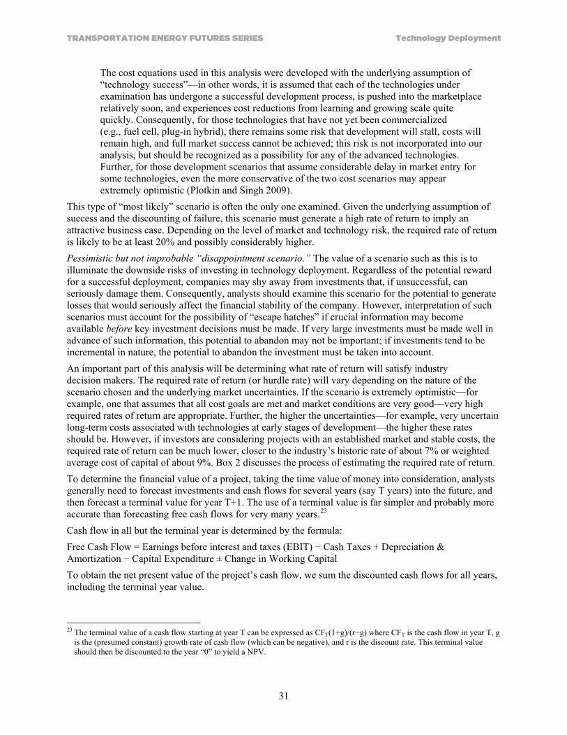
TRANSPORTATION ENERGY FUTURES SERIES Technology Deployment
31
The cost equations used in this analysis were developed with the underlying assumption of “technology success”—in other words, it is assumed that each of the technologies under examination has undergone a successful development process, is pushed into the marketplace relatively soon, and experiences cost reductions from learning and growing scale quite quickly. Consequently, for those technologies that have not yet been commercialized (e.g., fuel cell, plug-in hybrid), there remains some risk that development will stall, costs will remain high, and full market success cannot be achieved; this risk is not incorporated into our analysis, but should be recognized as a possibility for any of the advanced technologies. Further, for those development scenarios that assume considerable delay in market entry for some technologies, even the more conservative of the two cost scenarios may appear extremely optimistic (Plotkin and Singh 2009).
This type of “most likely” scenario is often the only one examined. Given the underlying assumption of success and the discounting of failure, this scenario must generate a high rate of return to imply an attractive business case. Depending on the level of market and technology risk, the required rate of return is likely to be at least 20% and possibly considerably higher. Pessimistic but not improbable “disappointment scenario.” The value of a scenario such as this is to illuminate the downside risks of investing in technology deployment. Regardless of the potential reward for a successful deployment, companies may shy away from investments that, if unsuccessful, can seriously damage them. Consequently, analysts should examine this scenario for the potential to generate losses that would seriously affect the financial stability of the company. However, interpretation of such scenarios must account for the possibility of “escape hatches” if crucial information may become available before key investment decisions must be made. If very large investments must be made well in advance of such information, this potential to abandon may not be important; if investments tend to be incremental in nature, the potential to abandon the investment must be taken into account. An important part of this analysis will be determining what rate of return will satisfy industry decision makers. The required rate of return (or hurdle rate) will vary depending on the nature of the scenario chosen and the underlying market uncertainties. If the scenario is extremely optimistic—for example, one that assumes that all cost goals are met and market conditions are very good—very high required rates of return are appropriate. Further, the higher the uncertainties—for example, very uncertain long-term costs associated with technologies at early stages of development—the higher these rates should be. However, if investors are considering projects with an established market and stable costs, the required rate of return can be much lower, closer to the industry’s historic rate of about 7% or weighted average cost of capital of about 9%. Box 2 discusses the process of estimating the required rate of return. To determine the financial value of a project, taking the time value of money into consideration, analysts generally need to forecast investments and cash flows for several years (say T years) into the future, and then forecast a terminal value for year T+1. The use of a terminal value is far simpler and probably more accurate than forecasting free cash flows for very many years.23 Cash flow in all but the terminal year is determined by the formula: Free Cash Flow = Earnings before interest and taxes (EBIT) − Cash Taxes + Depreciation & Amortization − Capital Expenditure ± Change in Working Capital To obtain the net present value of the project’s cash flow, we sum the discounted cash flows for all years, including the terminal year value.
23 The terminal value of a cash flow starting at year T can be expressed as CFT(1+g)/(r−g) where CFT is the cash flow in year T, g
is the (presumed constant) growth rate of cash flow (which can be negative), and r is the discount rate. This terminal value should then be discounted to the year “0” to yield a NPV.

Technology Deployment TRANSPORTATION ENERGY FUTURES SERIES
32
Box 2. Estimating Required Rate of Return Arguably the most important piece of information needed to perform a project valuation is an appropriate required rate of return (RRR). If the RRR is used as a discount rate to determine the net present value (NPV) of all the investments into a project and free cash flows from a project, whenever they occur, the project should be considered to have passed its initial investment hurdle if the NPV>0.
The RRR may be expressed in the form:
RRR = WACC + ru
where WACC is the automotive industry’s weighted cost of capital from all sources, and ru is the project-specific risk.
One source of estimates of industry-average WACC is a website supported by Aswath Damodaran, professor of finance at the Stern School of Business at New York University (Damodaran 2009). His estimates use the Value Line database of 5,928 firms. Based on his data, WACC for the automotive industry (vehicle manufacturers plus suppliers) during the past decade or so averages about 9%, as indicated in Figure B.2 (see also http://pages.stern.nyu.edu/~adamodar/New_Home_Page/datafile/wacc.htm).
Figure B.2. Weighted average cost of capital
in the automotive industry, 1998–2010 Estimating project-specific risk ru, the premium for risks unique to the investment project, requires judgment on the part of the analyst or forecaster. The project-specific risk reflects only how risky the project is relative to the financial market risk facing the automotive industry or other investor contemplating an automotive investment in new technology. Some guidance can be provided by considering that the discount rates (equivalent to RRR) used by venture capitalists and investment banks are very high. Discount rates used are in the range of 20–100% according to Timmons and Spinelli (2004) or 40–75% according to Westland (2002). This suggests that investors identify an element of unique specific risks and attempt to extract a penalty for this risk. However, as noted previously, we are primarily interested in investments occurring after the initial part of the development cycle, where uncertainty is lower. An initial estimate of the range of ru is 10–30%, depending on the risk factors associated with the investment and the degree of optimism associated with estimates of costs and prices. However, this range is basically an educated guess, and there would be substantial benefit from surveying automotive industry economists and economic analysis departments to establish a more credible estimate.
Factors that determine the project-specific risk for automotive projects are:
• Whether estimates of cash flow are derived using “expected values” of investment costs, sales, and prices or optimistic values. In other words, cash flow estimates using optimistic assumptions should be evaluated using a higher required rate of return than if the cash flow estimates are made using more skeptical assumptions.
• Evidence of a clear market for the technology. Technologies that demand that consumers change their behavior (e.g., limit trips to short lengths, or plan for long refueling times) or take a leap of faith that there will be a decent resale market for used vehicles — or involve some other factor that adds to market uncertainty — will require a higher RRR until these issues are resolved.
• Robustness of cost and performance estimates. Technologies at an early stage of development with current high costs and uncertain performance under real-world conditions are dependent on substantial learning to clear market hurdles. The distance between current cost and performance and long-range targets will strongly affect RRR.

TRANSPORTATION ENERGY FUTURES SERIES Technology Deployment
33
To determine whether the rate of return of the project’s investments exceeds the required rate of return (RRR) or hurdle rate, analysts can either:
• Calculate the discounted net present value (NPV) of the project (treated as a single management decision) with the RRR used as a discount rate. If the NPV > 0, the RRR has been exceeded.
• Calculate the discount rate that, applied to the cash flows, would give an NPV of zero.24 This result is the rate of return of the project, and should exceed the RRR.
If multiple scenarios are examined, assigning probabilities to the scenarios and applying them to the individual scenario cash flows allows the calculation of an expected NPV. 3.3.4. Decision Tree Analysis Method 1 may fail to account for some important options available to the industry to mitigate risks. In particular, the method tends to treat the investments embedded within a scenario as a chain of events that occur inexorably over time. In reality, as noted above, investors are rarely incapable of adjusting their strategy over time as new information becomes available. They can abandon a project, delay investments to wait for better conditions or more information, change the scale of future investments, and so forth, and all of these options add to the expected value of an investment scenario involving multiple investment decisions over time. When cash flow analysis is used to explore the consequences of future conditions less favorable to a project’s success (e.g., in risk analysis), it can yield a result that is overly pessimistic for major investments that occur over time and in stages unless it accounts for the multiple options in individual scenarios. Two methods used by industry and financial analysts to account for these options are Real Options Analysis (Evans and Zhang 2009; Kester 1984; Myers 1984; Sanislo 2003; Schneider et al. 2008) and Decision Tree Analysis (Behn and Vaupel 1982; Steffens and Douglas 2007; Boer 2003). Real Options Analysis using the work of Merton (1973) and Black and Scholes (1973) has the advantage over Decision Tree Analysis of taking account of changing risk over time (with reduced discount rates over time as risk declines), but it is ill-suited for risky projects where historical data on risks are not available (Neely and de Neufville, in press). The method suggested here is Decision Tree Analysis. A number of analysts have begun to advocate the use of Decision Tree Analysis and other related methods for evaluating automotive projects. For example, Kromer (2006) has evaluated lithium ion versus nickel-metal-hydride battery use in hybrid vehicle drivetrains using a two-stage decision tree. MacKenzie (2007) has examined the value of fuel flexibility (ethanol capability) in automobiles, also using a two-stage decision tree. Basically, what Decision Tree Analysis implies is that an investment project is broken down into its basic parts—capital investments, decision points about how to proceed, and uncertainty points where paths may diverge because of different conditions (e.g., markets are friendly or unfriendly toward a technology)—and these parts are drawn onto a diagram that resembles a tree with gradually expanding branches. In the tree, time proceeds from left to right. The various possible pathways that the investment can take are identified (in a simplified manner) by the following:
• The tree begins with the leftmost “trunk” called a “root node”—it represents the point at which a decision maker is faced with an investment choice or an uncertainty. The hoped-for outcome of building the tree is to determine what a risky investment (or series of investments) is worth.
• The tree begins to branch out at key event or uncertainty nodes (designated by circles) when an uncertainty is resolved (e.g., when it becomes clear that the market is favorable or unfavorable, an uncertain regulatory issue is resolved, etc.) and decision nodes (designated by small squares), where key decisions must be made (e.g., whether to invest in a new assembly line); end nodes of
24 This discount rate may have to be estimated by trial and error if software to accomplish this calculation is not available.

Technology Deployment TRANSPORTATION ENERGY FUTURES SERIES
34
each final branch of the tree are designated by triangles. For example, the decision tree shown in Figure 3.2 represents a case where two sequential investments are made, with the second occurring after new information will become available about market conditions. The sequencing of investments will allow the investor to choose whether or not the second investment will be made in the face of this new information.
Figure 3.2. Simple decision tree showing two-stage investment
In the decision tree, probabilities are given for each branch out of an uncertainty node, for example, 50% for good or poor markets in the figure. A decision tree is built by going through the following steps25:
1. Divide the analysis into risk phases. For automotive technology investments, analysts might start with the decision to establish a research project into a new technology, but it is recommended here that the decision tree begin at a later phase. One possibility is to begin with the decision to bring out an introductory niche vehicle. Additional later risky decisions might involve developing and marketing a more mainstream mass-market vehicle to be manufactured in large quantities, and later, introducing the technology throughout the company’s model line. Analysts must carefully assign likely dates to the nodes (e.g., when choices must be made).
2. Identify the critical uncertainties. For automotive technologies, important uncertainties include oil (or gasoline) prices; technology cost and performance outcomes; government policy decisions (e.g., CAFE rules, technology subsidies); and the status of the competition (i.e., conventional ICE-based drivetrain vehicles). Accounting for all uncertainties independently would yield an impossibly complex tree, so these uncertainties must be reduced to a subset of only a few, perhaps combining some uncertainties into a single expression of probability. It is useful here to consider which uncertainties are most likely to affect the outcomes of the investments at different stages of the tree—for example, the success of a niche vehicle may depend primarily on the performance of the technology, whereas the success of a mass-market vehicle will also depend on costs and probably on gasoline prices. Analysts must assign dates to when the key uncertainties may be resolved (e.g., when the market’s response to early vehicles becomes clear).
25 This discussion of the Decision Tree Analysis methodology borrows extensively from Damodaran (2009).
First investment Decision
Uncertainty point: What kind of market? Second investment decision

TRANSPORTATION ENERGY FUTURES SERIES Technology Deployment
35
3. Draw the outline of the tree with decision and chance nodes. This step can be completed using the outcomes of 1 and 2.
4. Estimate probabilities of outcomes. The analyst should keep two things in mind here: the probabilities for each phase must sum to one, and the probabilities may depend on earlier outcomes (e.g., the market friendliness towards a mass-market vehicle will likely depend on information about the market success of the niche vehicle).
5. Fill in the investments made, in real dollars and net present values (discounted to year 0). These values can be entered into a cash flow table as illustrated in the example below, Figure 3.3.
6. Estimate cash flows at relevant nodes,26 in real dollars and NPV. These values are also entered into the cash flow table. They are also entered into the tree in the boxes, as shown in Figure 3.4. Note that net cash flows include both investments (as negative cash flows) and cash generated by those investments when both occur in the same segment of the tree. When entering the investments and generated cash into the tree, it is important to avoid double-counting the investments—the cash generated by the investments should include the net of sales revenues minus only variable costs (i.e., analysts should not also subtract amortized investment costs or mortgage costs from the sales revenues, because these costs are already accounted for by the original investment).
7. Estimate the terminal values of each of the rightmost branches of the tree. These terminal values, entered to the right of each end node (triangle), are the net present values of the cash flows (including investments) of each of the branches, from year zero to the year embodied by the end node.
8. Assign values to the tree (“rolling up the tree”). Working from right to left, the “values of the branch” must be estimated at each point prior to (that is, to the left of) each decision or uncertainty/event node. For a decision node, the value is the maximum of the branches to the right of the node. The maximum is chosen because a decision maker will always choose the path that offers greater value. For an event/uncertainty node, the value is the expected value of the multiple branches to the right (that is, occurring later in time). This is where the probabilities are taken into account.
Decision tree analysis can seem complex, although there is spreadsheet software available to make the process more automated and organized.27 Further, the estimation of the components of cash flow is no simple matter, and demands multiple assumptions. Nevertheless, once the initial process is completed, having the tree available in spreadsheet form allows sensitivity analysis to be readily performed. In other words, it will be possible to examine how the financial viability of the project changes with changing assumptions about investment magnitude and timing, probabilities of market success, and so forth. Decision Tree Example 1: Option to Abandon An illustration of a simple decision tree analysis, to demonstrate the methodology, has an automotive manufacturer facing a two-stage investment opportunity with the option to abandon after the first stage, as shown above in Figure 3.2. Stage 1 requires an investment of $750 million (year 1) to acquire the rights to a particular brand name, but there are no free cash flows unless the firm invests an additional $1 billion in a new plant in Stage 2 (year 2) to produce vehicles under the brand. In Stage 2, it would take the buyer one year to build the plant and begin sales. Before Stage 2 investments, information about the strength of the market will be available. There is a 50% chance of a
26 Estimates must be made wherever cash flows emerge: for example, investments count as negative cash flows, and cash flows
from sales emerge after an event node establishing a good or poor market. 27 For example, TreePlan, www.treeplan.com.

Technology Deployment TRANSPORTATION ENERGY FUTURES SERIES
36
good market, in which case, the auto manufacturer will earn $3 billion, and a 50% chance of a poor market in which case earnings will be only $1 billion. Investments and cash flows28 shown in Table 3.1 are in millions of dollars. WACC is assumed to be 9%.
Table 3.1. Cash Flow Table for “Option to Abandon” Case Nominal Values (in Money of the Day) Present Values (in Money of Year 0)
Stage Year Make Second Investment Abandon Discount Multiplier
for WACC= Make Second Investment Abandon
Investment Good
Market Poor
Market Investment Good
Market Poor
Market 9% Investment Good
Market Poor
Market Investment Good
Market Poor
Market
1 0 $0 $0 $0 $0 $0 $0 1.00000 $0 $0 $0 $0 $0 $0
1 ($750) $0 $0 ($750) $0 $0 0.91743 ($688) $0 $0 ($688) $0 $0
2 2 ($1,000) $0 $0 $0 $0 $0 0.84168 ($842) $0 $0 $0 $0 $0
3 $0 $3,000 $1,000 $0 $0 $0 0.77218 $0 $2,317 $772 $0 $0 $0
Present Value Totals: ($1,530) $2,317 $772 ($688) $0 $0
The table is constructed so that its rows show values in years zero through three, with the “choose to make the second investment/abandon the project” nominal values for investments and cash flow side by side on the left, and the present values on the right.
Figures 3.3 and 3.4 show how populating the tree with cash flow entries is begun, by first inserting present values of investments (Figure 3.3) and then net cash flows (Figure 3.4) as they appear in the totals section of the table. For example, in the uppermost branch of the tree, the first investment (circle 1) comes before the uncertainty node, and the second investment (circle 2) and net cash flows (circle 8) come after.
28 As noted earlier, the net cash flows represent the net of revenues minus variable costs; the investment costs are entered
separately into the table, so amortized investment costs or mortgage costs must not be included in the net cash flows entered in the other columns of the table (and entered in the tree).

TRANSPORTATION ENERGY FUTURES SERIES Technology Deployment
37
Figure 3.3. Inputting investments into the decision tree
Figure 3.4. Inputting the cash flows into the decision tree

Technology Deployment TRANSPORTATION ENERGY FUTURES SERIES
38
Figure 3.5 shows how the terminal values are calculated, by adding the investments and net cash flows from the beginning of the tree to each terminal node.
Figure 3.5. Inputting the terminal values to the decision tree
For each terminal point, add up the investments and cash flows on the branches from the start of the tree to that point
$787 = ‒$688 + $0 ‒ $ 842 + $2,317
‒$688 = ‒$688 + $0 + $0 + $0
‒$758 = ‒$688 + $0 ‒ $842 + $772
‒$688 = ‒$688 + $0 + $0 + $0
($688)
Good Market
Poor Market
Make 2nd Investment
Make 2nd Investment
First Stage Investment
Abandon
Abandon
$0
$0
50%
50%
$2,317
Second Stage
$772
$0
$0
$0
$0
($842)
($842)

TRANSPORTATION ENERGY FUTURES SERIES Technology Deployment
39
Finally, Figure 3.6 shows how the tree is valued, by moving from right to left and using either the expected values (for event/uncertainty nodes) or maximum of the branch values (for decision nodes). In Figure 3.6, the overall value of the tree is positive—$49 million—so that the investment has an expected value higher than zero… or, in other words, the investment is expected to earn a higher rate of return than the industry’s weighted average cost of capital. In this example, the option to abandon the project before committing to the second investment adds significant value, which can be estimated from the value of the tree without the branches for the “Abandon” options, that is, 0.50 × $787 million − 0.5 × $758 million or $15 million. So the option to abandon is the difference between $49 million and $15 million, or $34 million. It is often the case that the option to abandon the project can be extremely valuable, and not accounting for it can yield a misleadingly low value for the investment scenario.
Figure 3.6. Assigning values to the decision tree
Good Market
Poor Market
Make 2nd Investment
Invest
Abandon
Abandon
50%
50%
Working from right to left compute the “value of the branch” at each point prior to a decision or an uncertainty. For a decision node, the “value of the branch” is the maximum of the values of the immediately subsequent branches. For an event node, the “value of the branch” is the expected value of the values of the immediately subsequent branches.
($758)
($688)
($688)
$787
1
2
$49
$787
($688)$49 = (0.50)($787) + (0.50)(‒$688)
An Event Node: The value of the node is the expected value of the possible outcomes. The value of the Good Market outcome is $787, and the value of the Poor Market outcome is ‒$688. Since each outcome has a 50% probability of occurring, the value of the node is (0.50)($787) + (0.50)*(‒$688) = $49. This is the expected value of the Tree.
A Decision Node: count the branches from the top to the bottom. "Make 2nd Investment " is 1 and has a branch value of $787. “Abandon" is 2 and has a branch value of ‒$688. A value-seeking investor would choose the branch with the highest value. Here, the highest value would result from branch 1, “Make 2nd Investment”. This is the resulting value of the Good Market branch, $787. The value in the square shows the chosen branch, 1 (Make 2nd Investment).
A Decision Node: count the branches from the top to the bottom. "Make 2nd Investment " is 1 and has a branch value of ‒$758. “Abandon" is 2 and has a branch value of ‒$688. A value-seeking investor would choose the branch with the highest value. Here, the highest value would result from branch 2, “Abandon". This is the resulting value of the Poor Market branch, ‒$688. One may question why a branch with a negative value is chosen, but at this point the 1st investment is a sunk cost (and is included in the terminal values of both branches), and the only choices available are to Make the 2nd investment or Abandon, so the least negative branch is chosen.The value in the square shows the chosen branch, 2 (Abandon).
$787 = MAX($787, ‒$688)
‒$688 = MAX(‒$758,‒$688)
($688)
11
11
12
12
13
13
$0
$0
$2,317
$772
$0
$0
($842)
($842)

Technology Deployment TRANSPORTATION ENERGY FUTURES SERIES
40
Decision Tree Example 2: Moving from a Low-Volume to a High-Volume Market In this example, we consider a hypothetical automotive investment project and compare the two main valuation methods, Expected NPV and Decision Tree Analysis. Here, an automaker can test the market with a low-volume model using a new powertrain technology before deciding whether to scale up production of a high-volume model of similar design. The market for the low-volume model is assumed to be an indicator—though not a guarantee—of the market for the high-volume model. The automaker can use information from the low-volume model to decide about scaling up for the high-volume model. The decision tree for this example is shown in Figure 3.7.
Decision Tree for Low Volume to High VolumeDecision node
Event or uncertainty node
Terminal point Good Market
Poor Market
High Volume Model
Low-volume Model
Abandon
60%
40%
First investment decision
Second investment decision
Event node: What kind of market for low-volume model?
Good Market
Poor Market20%
80%
Abandon
High Volume Model
Abandon
Good Market
Poor Market
10%
90%
Event node: What kind of market for high-volume model?
Figure 3.7. Decision tree for low-volume to high-volume vehicle decisions

TRANSPORTATION ENERGY FUTURES SERIES Technology Deployment
41
The automaker can bring the low-volume model to market by investing $700 million per year for three years. Launched in the third year of the project, the life cycle of the low-volume model would be six years. Sales revenues from the low-volume model will depend on market conditions, with a 40% probability of a good market and a 60% probability of a poor market. In year 6, market results for the low-volume model will be known, and the automaker will decide whether to scale up production of the high-volume model at a cost of $900 million per year for three years. If the low-volume market is good, then there is an assumed 80% probability that the market for the high-volume model will be good and a 20% probability that it will be poor.29 If the market for the low-volume model is poor, then the chance for a good market for the high-volume model is assumed to be only 10%. The 20% probability of a poor market for the high-volume model even after a successful low-volume market launch is associated with the need to market the high-volume vehicle to different consumers who have different market values. There is also some probability that, in the time between the two launches, the overall market for vehicles could have declined. However, the risk of an overall adverse market is already embodied in the 9% discount rate and should not be incorporated in the branch probabilities in the decision tree. The 10% probability of a good market for the high-volume model even after a poor low-volume market is associated with the combination of the different consumer market segments being targeted and the likelihood that the high-volume vehicle can be priced lower (because of lower costs from larger-scale production and learning benefits from the earlier low-volume production). The automaker must first decide whether to pursue the low-volume market. If it does, then once the market conditions for the low-volume model are known, it can decide on whether to scale up production of the high-volume model. The investments needed to launch the models, shown in Table 3.2, are assumed to be independent of market outcomes, that is, they are the same for “Good Market” and “Poor Market.”
Table 3.2. Investments Required for Production of the Low-Volume Model and the High-Volume Model, Nominal and Present Values at a Cost of Capital of 9%
Investments, Nominal $ Investments, Present Value (PV)
Year Low Volume High Volume Discount factor
(@ 9%) Low Volume High Volume 0 ($700) 0 1.0 ($700) 0 1 ($700) 0 0.9174 ($642) 0 2 ($700) 0 0.8417 ($589) 0 3 0 0 0.7722 0 0 4 0 0 0.7084 0 0 5 0 0 0.6499 0 0 6 0 ($900) 0.5963 0 ($537) 7 0 ($900) 0.5470 0 ($492) 8 0 ($900) 0.5019 0 ($452) 9 0 0 0.4604 0 0
10 0 0 0.4224 0 0 Total ($1,931) ($1,481)
29 Some technologies may be attractive to “early adopters,” a small portion of the market, yet be unattractive to more mainstream
consumers.

Technology Deployment TRANSPORTATION ENERGY FUTURES SERIES
42
Next we develop cash flows. These might come from sales projections for different market outcomes. These numbers used here are hypothetical. For the low-volume model, in a good market, cash flows will be $400 million starting in year 4 and decrease by 5% each year for six years (the planned life of this model). In a poor market, cash flows from the low-volume model are zero, implying that revenues from vehicle sales are sufficient to cover only the variable costs of production. These results are shown below in the second and third columns in Table 3.3. Present values, or PVs (in year 0) of these cash flows are shown in columns 6 and 7. Cash flows for the high-volume model under a good market start in year 10 at $2.0 billion and decrease by 5% each year thereafter (column 3, below). The cash flow shown in year 10 is the terminal value of continued production of the high-volume model. This was estimated assuming that cash flows for year 10 and the following years continue decreasing 5% each year. The value of this cash flow stream in year 10 is the terminal value, TV (or the “horizon” value) and is given (see Brealey, Myers, and Allen 2006, p. 510) by:
𝑇𝑉 =𝐶10
𝑊𝐴𝐶𝐶 − 𝑔
where: TV is the value of the cash flows for year 10 and all subsequent years C10 is the cash flow for year 10 (not including subsequent years) = g C9 g is the growth rate (‒5% in this example) WACC is the cost of capital (9% in this example)
The present values of the cash flows for the high-volume model under a good market are in column 8. In a poor market, the high-volume model generates zero cash flow (columns 5 and 9).
Table 3.3. Net Cash Flows (Not Counting Investments) from the Low-Volume Model and the High-Volume Model, Nominal and Present Values at a Cost of Capital of 9%
Cash Flows (Nominal $) Cash Flows (Present Value @ 9%) Low-Volume Model High-Volume Model Low-Volume Model High-Volume Model
Year Good Mkt Poor Mkt Good Mkt Poor Mkt Good Mkt Poor Mkt Good Mkt Poor Mkt 0 $0 $0 $0 $0 $0 $0 $0 $0 1 $0 $0 $0 $0 $0 $0 $0 $0 2 $0 $0 $0 $0 $0 $0 $0 $0 3 $400 $0 $0 $0 $309 $0 $0 $0 4 $380 $0 $0 $0 $269 $0 $0 $0 5 $361 $0 $0 $0 $235 $0 $0 $0 6 $343 $0 $0 $0 $204 $0 $0 $0 7 $326 $0 $0 $0 $178 $0 $0 $0 8 $310 $0 $0 $0 $155 $0 $0 $0 9 $0 $0 $2,000 $0 $0 $0 $921 $0
10 $0 $0 $13,571 $0 $0 $0 $5,733 $0 Total PV: $1,351 $0 $6,654 $0

TRANSPORTATION ENERGY FUTURES SERIES Technology Deployment
43
The first step in filling in the decision tree is to input the (NPV of) investments, from the last line of Table 3.2, as shown below in Figure 3.8. The investment values are entered after the decision nodes (small boxes).
Figure 3.8. Inputting the investments into the decision tree
Input the InvestmentsAfter each decision node, enter the investments (discounted to present value). These are from the “Total PV” row in the Investments table.
1
1
Investments, PV
Low Vol High Vol
Total PV: ($1,931) ($1,481)
Good Market
Poor Market
High Volume Model
Low-volume Model
Abandon
60%
40%
Good Market
Poor Market20%
80%
Abandon
High Volume Model
Abandon
Good Market
Poor Market
10%($1,931)
2
($1,481)
($1,481)
2
The investments are assumed to be independent of market outcomes, so they are the same for “good market” or “poor market.”
2
90%
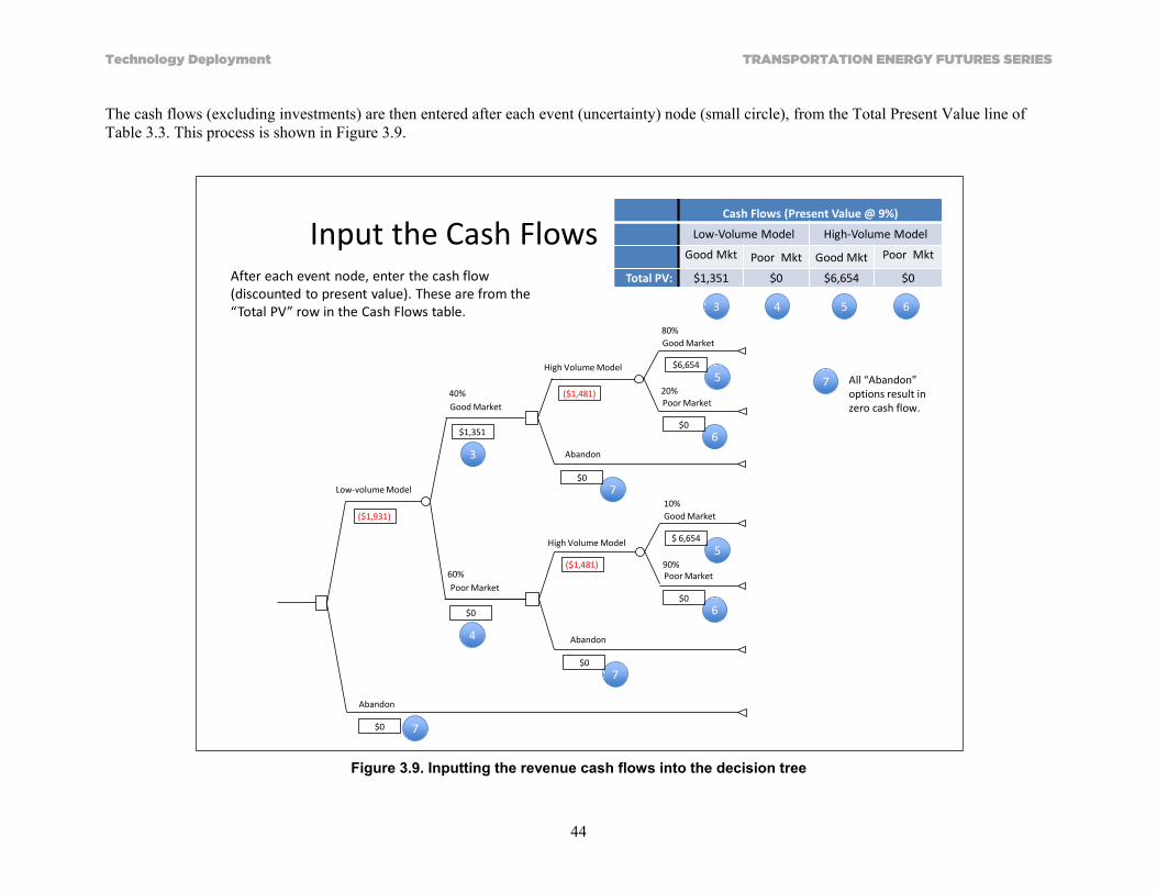
Technology Deployment TRANSPORTATION ENERGY FUTURES SERIES
44
The cash flows (excluding investments) are then entered after each event (uncertainty) node (small circle), from the Total Present Value line of Table 3.3. This process is shown in Figure 3.9.
Figure 3.9. Inputting the revenue cash flows into the decision tree
Input the Cash FlowsAfter each event node, enter the cash flow (discounted to present value). These are from the “Total PV” row in the Cash Flows table. 3
3
4
7
5
7
Good Market
Poor Market
High Volume Model
Low-volume Model
Abandon
60%
40%
Good Market
Poor Market20%
80%
Abandon
High Volume Model
Abandon
Good Market
Poor Market
10%($1,931)
4
($1,481)
($1,481)
6
Cash Flows (Present Value @ 9%)
Low-Volume Model High-Volume Model
Good Mkt Poor Mkt Good Mkt Poor Mkt
Total PV: $1,351 $0 $6,654 $0
$1,351
$0
5$6,654
6$0
5$ 6,654
6$0
90%
7$0
7$0
$0
All “Abandon” options result in zero cash flow.

TRANSPORTATION ENERGY FUTURES SERIES Technology Deployment
45
Next, as shown in Figure 3.10, the terminal values of each end branch of the tree are calculated by adding up the investments (negative values) and (positive) cash flows of the entire branch, starting with initial investments at the beginning of the tree.
Figure 3.10. Inputting the terminal values to each end branch of the decision tree
Input the Terminal ValuesFor each terminal point, add up the net cash flows on the branches from the start of the tree to that point
$4,592 = ‒$1,931 + $1,351 ‒ $1,481 + $6,654
Good Market
Poor Market
High Volume Model
Low-volume Model
Abandon
60%
40%
Good Market
Poor Market20%
Abandon
High Volume Model
Abandon
Good Market
Poor Market
10%($1,931)
($1,481)
($1,481)
$1,351
$0
$ 6,654
$0
$ 6,654
$0
90%
$0
$0
$0
‒$2,061 = ‒$1,931 + $1,351 ‒ $1,481 + $0
‒$581 = ‒$1,931 + $1,351 + $0
$3,242 = ‒$1,931 + $0 ‒ $1,481 + $6,654
‒$3,412 = ‒$1,931 + $0 ‒ $1,481 + $0
‒$1,931 = ‒$1,931 + $0 + $0
$0
80%

Technology Deployment TRANSPORTATION ENERGY FUTURES SERIES
46
Finally, values are assigned to each node of the tree by working from right to left in the following manner:
• Before each decision node, the value is the maximum of the branches to the immediate right of the node… since decision makers will choose that branch with the highest value.
• Before each event/uncertainty node, the value is the expected value of the branches to the immediate right of the node, that is, the sum of (value of the branch) times (fractional probability of the branch).
The process is shown in Figure 3.11. The ultimate value of the decision tree, shown at the left in Figure 3.11, is $146 million, implying that the automaker should consider this investment as viable. An alternative means of valuing the investment, expected NPV, does not consider the possibility of abandoning the venture in the face of a poor market. Calculating the value of the investment this way changes the value of the poor market branch from ($1,931), or the value of abandoning the project, to ($2,747), the value of continuing the project even in the face of a poor market. The overall value of the tree would then become
0.40 × $3262 + 0.60 × ($2747) = ($343) In other words, the value of abandonment is $146 million – ($343 million) = $489 million, and ignoring this value shifts the apparent value of the investment from moderately positive (i.e., viable) to overwhelmingly negative.

TRANSPORTATION ENERGY FUTURES SERIES Technology Deployment
47
Figure 3.11. Assigning values to each node of the tree and to the entire tree

Technology Deployment TRANSPORTATION ENERGY FUTURES SERIES
48
3.4. Conclusions The discussion and examples above illustrate the value of examining potential technology rollouts from the viewpoint of the investor. Examining the cash flow of a potential investment, especially in a decision tree format, forces the analyst to consider the length of time before a project will break even and begin to pay out, and the potential for alternative (and negative) outcomes to the “most likely” or “best” cases that are often the subject of scenario analysis. In other words, construction of a decision tree forces the analyst to consider risk, a crucial factor in investor decision-making. Of course, there is no guarantee that this consideration will be accurate or that it will reflect the likely view of industry; analysts undertaking this kind of project evaluation must carefully consider the risk behavior of the investors most likely to participate in the investments under consideration. Another benefit of examining the cash flow in a decision tree format is that it explicitly includes the value of the option to abandon the project before all investments are made (where this option exists). Both examples demonstrate that this option can be very valuable, and may turn an investment from a “no go” to a “go” when the option is taken into account. A potential stumbling block of constructing a cash flow and decision tree analysis for a potential vehicle technology rollout is the need to develop capital cost estimates for the major components of the rollout. Although there is a rich literature about technology costs, this literature typically does not develop or specify capital cost estimates. As discussed in Section 4, the work of scenario analysts wishing to perform a cash flow analysis could be eased considerably by developing a library of capital cost estimates for the building blocks of a technology rollout. Another potential stumbling block is the complexity of industry technology development and rollout. Most vehicle manufacturers are now global manufacturers, and the largest suppliers are global as well—implying that analyses and scenarios with strict national boundaries can miss important investment factors such as global economies of scale and learning based on manufacturing across several nations. Addressing this level of complexity is beyond the scope of this report but is deserving of robust attention.

TRANSPORTATION ENERGY FUTURES SERIES Technology Deployment
49
4. FUTURE WORK
As noted in the introduction, this report is meant to serve as the beginning of a discussion about making vehicle deployment scenarios more robust. The discussion develops a timeline for vehicle technology deployment and describes a method of cash flow and decision tree analysis designed to account for the viewpoint of potential investors in new technology and to introduce an accounting of risk into scenario analysis. This section describes additional analyses in three areas that could facilitate use of these tools. 4.1. Building a Database of Basic Vehicle Investments As noted earlier, the use of cash flow and decision tree analysis as a means to “reality test” scenarios requires a considerable effort to define the building blocks of a scenario, develop a timeline for investments and cash flows, and judge the probability of outcomes (if “expected” cash flows or decision trees are desired). One crucial element of this process is to estimate the magnitude of the investments needed for a scenario. This process would be assisted considerably by developing a database of investment costs for the afore-mentioned building blocks. Although there are multiple reports that focus on estimating the costs of future vehicle technologies (e.g., Plotkin and Singh 2009; Bandivadekar et al. 2008; NRC 2011; EPA 2011), these reports tend to avoid developing their cost estimates by explicitly evaluating the capital costs of the major components of manufacturing—and thus do not identify these costs.30 Furthermore, the technology costs identified by these reports implicitly include the “per unit” cost of capital as a fraction of the total technology cost, but generally this fraction is not specifically broken out. In calculating cash flow and building a decision tree, the net cash flow values that are separate from investments are based on revenues minus variable costs (e.g., the fraction representing capital costs must be subtracted from the technology cost estimates provided by most reports). Lack of a database on the capital costs associated with developing and manufacturing new technologies will greatly complicate the task of conducting cash flow analyses and building decision trees. An effort to build a database of capital costs would identify reports that specifically address capital requirements. For example, Nelson et al. (2011) identify the capital costs for lithium-ion manufacturing facilities; Table 4.1 comes from this source.
Table 4.1. Sample Table of Lithium Ion Capital Costs
Baseline Double Power
Double Capacity
Double Modules
Calculated Battery Parameters Battery energy storage, kWh 8.7 8.8 17.3 17.4 Battery power at target % OCV, kW 50.0 100.0 86.9 100.0 Required battery power, kW 50.0 100.0 50.0 100.0 Capacity, Ah 40 40 80 40 Number of cells 60 60 60 120 Battery weight, kg 59.1 72.4 108.2 116.0 Battery volume, L 31.2 37.1 55.2 59.7
30 EPA (2011), which is by far the most detailed of the cost analyses, uses “indirect cost multipliers” to cover items such as
engineering, design and testing costs, and tooling costs.

Technology Deployment TRANSPORTATION ENERGY FUTURES SERIES
50
Baseline Double Power
Double Capacity
Double Modules
Calculated Battery Parameters (cont’d) Weight and volume of components exterior to battery
Weight, kg 11.0 9.0 11.0 9.0 Volume, L 5.6 4.0 5.6 4.0
Cooling system power requirement, W 1760 649 857 724 Vehicle electric range, miles 20.3 20.5 40.5 40.6
Investment Costs Capital equipment cost including installation, mil$ 127 149 161 212 Building, land and utilities
Area, m2 15,374 18,165 19,204 24,284 Cost, $/m2 3,000 3,000 3,000 3,000 Building investment, mil$ 46.1 54.5 57.6 72.9
Launch costs Rate: 5% of direct annual materials + 10% of other annual costs
Total, mil$ 10.62 13.11 17.05 19.30 Working capital (30% of annual variable costs), mil$ 28.78 35.80 47.53 53.28 Total investment, mil$ 212.53 252.58 283.32 357.74
(Source: Nelson et al. 2011)
4.2. Incorporating Cash Flow and Decision Analysis into Complex Projection Models
A second area of suggested future work is the examination of existing computer models often used to develop and evaluate scenarios of future energy development, and the development of methods to allow those models to incorporate some parts of the methodologies discussed here. Some of the relevant models are:
• NEMS, the National Energy Modeling System (U.S. Energy Information Administration and others)
• MARKAL (EPA and others)
• HyTrans, the Hydrogen Transition Model (Oak Ridge National Laboratory)
• AMIGA (Argonne National Laboratory) After an initial examination, these models do not appear to undertake the assessment of automotive industry decision-making under risk. They all seem to assume that vehicle manufacturers take a standard markup over actual costs or attain a return on investment at historic levels31 unless fuel economy or CO2 standards force them to absorb higher costs, or unless the scenarios of vehicle sales are specified exogenously (which may force manufacturers to absorb losses, at least as modeled). Manufacturer behavior is accounted for by a generalized set of rules, for example, rules that specify the scale at which manufacturing plants are built and the number of makes and models produced by those plants (assumed to be uniform throughout the industry). The actual fraction of vehicles of each type manufactured, when not externally provided, is assumed to be equivalent to vehicle sales of that type, which are determined by a VCM in which vehicle price is a key variable.
31 The models do not appear to account for the investment losses that would occur if market penetration of new technologies is
very low.
TRANSPORTATION ENERGY FUTURES SERIES Technology Deployment
51
The authors were able to examine the HyTrans model (Greene, Leiby, and Bowman 2007). In the model, the penetration of advanced vehicles like hydrogen FCVs is specified (as a scenario input) up to the year 2025, and vehicle sales after 2025 are determined by a VCM. Vehicle price is a crucial determinant of sales in the VCM, and that post-2025 price is based on a standard markup of estimated vehicle costs. These costs are determined by a calculation that depends on the attainment of long-term cost goals and on how far the technology has gone down the learning curves (based on earlier sales). In scenarios with optimistic cost assumptions, sales after 2025 will grow; in scenarios with less optimistic cost assumptions, sales may falter because vehicle prices will be higher than most consumers will accept (as modeled by the VCM). Vehicle sales are also a function of the number of makes and models offered, and this number is a function (within the model) of sales—the model assumes that vehicle manufacturing plants of a standard capacity offer a fixed number of models per plant, and these plants will produce up to capacity and then, as total sales grow, additional plants will be added, with each new plant allowing additional models to be offered. HyTrans calculates a measure of cash flow over time for the vehicle manufacturing industry, albeit in a constricted way. In the pre-2025 period, with externally provided vehicle sales, the VCM’s equations are used to determine what the vehicle prices would have had to have been to generate that level of sales, with actual vehicle costs estimated using the scenario cost assumptions and learning curves. Actual cash flow32 is calculated as the sum of vehicle price minus vehicle cost over all vehicle sales for each year, and will be negative until learning drives costs below price. For the post-2025 period, cash flow is also the sum of vehicle price minus cost for all sales, but during this period price is assumed to be based on a standard industry markup over cost, with sales determined by the VCM.33 In the HyTrans scenarios, even the scenarios with very optimistic costs, there initially is a long period of negative cash flow (with vehicle prices kept low to sustain sales) until learning eventually drives costs down to levels that will sustain sales growth even with prices that reflect normal manufacturer and dealer markups over cost (see the previous discussion of Figure 3.1). As noted, the model assumes that vehicle markups never exceed “standard” levels; thus, the losses incurred during the early years of sales growth are never recovered by higher-than-usual markups later on. In other words, the early losses must be made up either by industry accepting these losses as the price of staying in business, or by government subsidy. In fact, it is the underlying assumption in HyTrans that government will support the rollout of advanced vehicles until industry can proceed on its own. The idea that a future vehicle manufacturing industry may never be able to charge a higher-than-average markup for advanced technology does not appear to be unreasonable; if manufacturers did boost their markup, new market entrants presumably would be able to undercut their prices. The only way this scenario could be prevented is if the intellectual property associated with learning could be protected, so that new entrants would have to repay earlier entrants for access to that learning. Although the patent system can assure some protection, it is problematic whether it can protect the majority of the value gained through learning. With this methodology, HyTrans is essentially trying to answer the following question:
“If government will financially support sales of FCVs (or other advanced vehicles) until annual sales reach several million, and if industry accepts the challenge, can the industry be self-sustaining thereafter?”
A question that HyTrans in its current form is not trying to answer is, “Would industry be likely to sign on to such a project?” This is the question that we are in fact focusing on in this report.
32 Note that some analysts would object to HyTrans’s use of the term “cash flow” because the model’s estimates do not
incorporate estimates of actual capital expenditures. 33 Note that this calculation of cash flow does not directly consider investments in manufacturing facilities or other infrastructure,
relying entirely on estimates of vehicle costs and prices.
Technology Deployment TRANSPORTATION ENERGY FUTURES SERIES
52
4.3. Evaluating the Timing and Investment Context of Refueling Infrastructure Deployment Required for Advanced Vehicles
The deployment of some advanced vehicle technologies—battery EVs and HFCVs in particular, but even diesel vehicles if deployment is rapid—require simultaneous or even advanced deployment of a refueling infrastructure. The nature of these infrastructure components is quite specific to the technology. Diesel infrastructure primarily involves refinery modification and some addition to pumps and fuel storage at existing gas stations. Battery electric infrastructure involves the installation of slow charging stations primarily for residential recharge, but depending on the magnitude of the deployment and the underlying rationale for vehicle purchase, could involve large numbers of public charging stations and fast chargers; some electric utility investment in local transformers and generation capacity (especially if a great deal of peak charging is expected) would also be necessary. And hydrogen infrastructure likely involves building refueling stations and hydrogen production and distribution capacity in advance of vehicle sales, unless residential refueling becomes practical (e.g., with small natural gas reformers providing residential heat and electricity plus hydrogen). In addition, unless hydrogen vehicles are at first sold as “local vehicles,” many refueling stations will have to be built in areas where demand may build quite slowly to accommodate consumers’ desired travel flexibility. Timing issues for deploying alternative fuel infrastructure include the potential for community opposition to large production plants and refueling stations (especially if there are adverse safety perceptions), questions about labor availability (for rapid deployment), and others. If maximum deployment rates of this infrastructure are slower than similar rates for vehicles, the overall vehicle scenario will be slowed. Consequently, the overall timetable for advanced vehicle deployment should include consideration of both vehicle manufacture and sales, as well as refueling infrastructure development, where relevant. Similarly, evaluation of the business case for a vehicle technology rollout should include an examination of the refueling infrastructure investment requirements and development of cash flow and decision tree analyses for these investments. The types of investors and their risk avoidance characteristics may be quite different from that of vehicle manufacturing investors for some aspects of a refueling infrastructure. For example, integrated oil companies are quite familiar with multibillion-dollar investments that require a decade or more to generate cash flow; on the other hand, these companies will be far less likely than auto companies to perceive value from such investments outside of immediate sales of their product. Furthermore, some of the timing issues of fuel deployment, especially the effect of community opposition to stations and production plants, seem likely to be quite consequential to investment success and should be strongly considered in scenario analysis. Developing an analysis framework for refueling infrastructure will involve:
• Developing estimates of key timing events (e.g., fuel production plant construction time) and evaluating potential for delays.
• Identifying key investors, their required rates of return, and their level of risk aversion.
• For decision tree analysis, determining WACC (i.e., the weighted cost of capital) for key investors.
● Developing estimates of capital cost “building blocks” (e.g., refueling stations, large-scale production plants, etc.).

TRANSPORTATION ENERGY FUTURES SERIES Technology Deployment
53
5. CONCLUSIONS
Scenario development and analysis can serve multiple goals, ranging from very broad examinations of purely hypothetical futures to careful examination of possible solutions to critical problems; they can also serve to identify roadblocks to attaining future goals, by showing that those goals require specific actions that appear difficult or undesirable, or even unattainable. This report seeks to begin a conversation about adding an interesting component to scenario analyses generated to contemplate vehicle technology deployment—“reality checking” scenarios by careful consideration of the timing of stages of deployment and examination of the business case for deployment. Although it is likely that most scenario analyses contain a significant element of consideration of timing, this is rarely documented. A conclusion of this report is that many ambitious scenarios compress the timing of the earliest stages of development such that there is substantial risk that new technology vehicles could not penetrate the mass market within a given “allotted” time frame. Section 3 of this report, “Examining the Business Case,” addresses an issue that has not been much examined in the literature: whether the business community would likely make the investments needed for a given level of deployment. The overall suggestion of the report is that using cash flow analysis, especially in the creation of decision trees, is a useful approach to examining the business case. However, the development of a realistic cash flow analysis will take considerable effort, although this effort would be lessened by development of a library of capital cost estimates for the various building blocks of a technology deployment. In any case, this approach is not for everyone. It has strong limitations when analysts may be trying to develop scenarios for the distant future, because both the timing of investments and their costs will be very uncertain, and the economic climate in several decades is equally uncertain. The level of effort required may be excessive for scenario analyses meant as pure thought exercises, or as the initial probing of future options. Further, the global nature of the automotive industry and, especially, the role of global suppliers add an important level of complexity that will be difficult to account for. Nevertheless, addressing the issue of the existence of a business case forces the analyst to take business risk into account and to ask important questions about the feasibility of scenarios.

Technology Deployment TRANSPORTATION ENERGY FUTURES SERIES
54
REFERENCES
Alson, J. 2011. Personal communication from J. Alson, U.S. Environmental Protection Agency, April 20, 2011. Automotive News. 2012. Vellequette, L., “Can Humans Manage the New Technology Deluge?”; H. Gremel, “Like Its Rivals, Toyota Revises Product Development”; and L. Vellequette, “Chrysler Promises Suppliers Quick Decisions on New Ideas,” all in the April 23 issue. Bandivadekar, A., et al. 2008. On the Road in 2035, Laboratory for Energy and the Environment, Massachusetts Institute of Technology report LFEE 2008-05 RP, September. Behn, R.D., J.W. Vaupel 1982. Quick Analysis for Busy Decision Makers, Basic Books.
Black, F., M. Scholes 1973. “The Pricing of Options and Corporate Liabilities,” Journal of Political Economy, Vol. 81, May–June, pp. 637–54. Boer, F.P. 2003. Risk-Adjusted Valuation of R&D Projects, http://www.boer.org/files/2003.pdf. Brealey, R.A., S.C. Myers, F. Allen. 2006. Principles of Corporate Finance, 8th ed., New York: McGraw-Hill Irwin. Bureau of Transportation Statistics. 2011. National Transportation Statistics, Tables 1-11 and 1-12, http://www.bts.gov/publications/national_transportation_statistics/html/table_01_11.html. Christensen, C. 2003, The Innovator’s Dilemma, Harper Business Essentials. Craig, P.P., A. Gadgil, J.G. Koomey. 2002. “What Can History Teach Us? A Retrospective Examination of Long-Term Energy Forecasts for the United States,” Annual Review of Energy and the Environment. Damodaran, A. 2009. The Dark Side of Valuation: Valuing Young, Distressed, and Complex Businesses, 2nd Edition, FT Press. EPA (U.S. Environmental Protection Agency). (forthcoming). Technology, CO2 and Fuel Economy Trends Database. EPA. 2011. Light-Duty Technology Cost Analysis, Power-Split and P2 HEV Case Studies, prepared for EPA by FEV, Inc., EPA-420-R-11-015, November. EPA. 2009. Light-Duty Automotive Technology, Carbon Dioxide Emissions, and Fuel Economy Trends: 1975 Through 2009, EPA 420-R-09-014, November. EPA and NHTSA (U.S. Environmental Protection Agency and National Highway Traffic Safety Administration). 2011. Draft Joint Technical Support Document: Proposed Rulemaking for 2017–2025 Light-Duty Vehicle Greenhouse Gas Emission Standards and Corporate Average Fuel Economy Standards, EPA-420-D-11-901, November. EPA, et al. (U.S. Environmental Protection Agency, National Highway Traffic Safety Administration, and California Air Resources Board). 2010. Interim Joint Technical Assessment: Light-Duty Vehicle Greenhouse Gas Emission Standards and Fuel Economy Standards for Model Years 2017–2025, September. Evans, J.L., D. Zhang. 2009. “Real Options Evaluation of Financial Investment in Flexible Manufacturing Systems in the Automotive Industry,” Int. J. Automotive Technology and Management, Vol. 9, No. 3. German, J. 2009. “Lead Time, Customers, and Technology: Technology Opportunities and Limits on the Rate of Deployment,” in Sperling, D., and J. Cannon (eds.), Reducing Climate Impacts in the Transportation Sector, DOI:10.1007/978-1-4020-6979_5, @Springer Science+Business Media B.V. Greene, D.L., S.E. Plotkin. 2011. Reducing Greenhouse Gas Emissions from U.S. Transportation, Pew Center on Global Climate Change, January.

TRANSPORTATION ENERGY FUTURES SERIES Technology Deployment
55
Greene, D.L., P.N. Leiby, D. Bowman. 2007. Integrated Analysis of Market Transformation Scenarios with HyTrans, ORNL/TM-2007/094, Oak Ridge National Laboratory, June. Heywood, J. 2011. Personal communication from J. Heywood, Massachusetts Institute of Technology, October 11.
International Energy Agency. 2010. Energy Technology Perspectives 2010: Scenario & Strategies to 2050, http://www.iea.org/Textbase/nppdf/free/2010/etp2010_part1.pdf . Kester, W.C. 1984. “Today’s Options for Tomorrow’s Growth,” Harvard Business Review, 62(2), pp. 153–160. Kromer, M. 2006. Evaluation of Hybrid Vehicle Business Strategy, Massachusetts Institute of Technology, December, http://ardent.mit.edu/real_options/Real_opts_portfolio%20applications/ 2006%20Set/Kromer%20-%20Hybrid%20Vehicle.pdf. Lasher, S., S. Unnasch, M. Chan. 2004. “Hydrogen Infrastructure: Energy, Costs, and Transition,” 2004 Fuel Cell Seminar, San Antonio, TX, November 1–5, TIAX LLC. Also: S. Unnasch (2004). “Hydrogen Transition Model H2NowNPV,” Hydrogen Systems Modeling Workshop, University of California at Davis, September 20 (PowerPoint presentation); and S. Lasher (2005). “Fuel Choice for FCVs: Hydrogen Infrastructure Costs,” U.S. Department of Energy Merit Review, May 25, PowerPoint presentation.
MacKenzie, D. 2007. Valuation of Fuel Flexibility in a Vehicle Fleet, Sloan Automotive Laboratory, Massachusetts Institute of Technology, December, http://ardent.mit.edu/real_options/ Real_opts_portfolio%20applications/ESD%20material%20for%20posting%202007/ MacKenzie%20-%20Flex%20Fuel%20Vehicles%20-%20Complete.pdf.
Merton, R.C. 1973. “Theory of Rational Option Pricing,” Bell Journal of Economics and Management Science, Vol. 4, Spring, pp. 141–83. Moore, G.A. 2002. Crossing the Chasm, Harper Business Essentials, New York.
Murphy, J. 2010. Car Wars 2011–2014, Bank of America Merrill Lynch Industry Overview Report, May 26.
Myers, S.C. 1984. “Finance Theory and Financial Strategy,” Interfaces, 14(1), pp.126–137. Neely, J.E., III, R. de Neufville (in press). “Hybrid Real Options Valuation of Risky Product Development Projects,” International Journal of Technology, Policy, and Management. Nelson, P.A., et al. 2011. Modeling the Performance and Cost of Lithium-Ion Batteries for Electric Drive Vehicles, Argonne National Laboratory report ANL-11/32, September. NRC (National Research Council). 2011. Assessment of Fuel Economy Technologies for Light-Duty Vehicles, Washington, D.C.: The National Academies Press. NRC. 2008. Transitions to Alternative Transportation Technologies: A Focus on Hydrogen, Committee on Assessment of Resource Needs for Fuel Cell and Hydrogen Technologies, Board on Energy and Environmental Systems. Plotkin, S. 2007. Examining Hydrogen Transitions, Argonne National Laboratory report ANL-07/09, February. Plotkin, S., M. Singh. 2009. MultiPath Transportation Futures Study: Vehicle Characterization and Scenario Analysis, Argonne National Laboratory report ANL/ESD/09-5, July 22. Rogers, E.M. 2003. Diffusion of Innovations, 5th ed., Free Press, New York. Sanislo, M. 2003. Real Options and Monte Carlo Modeling for New Product Development, PowerPoint presentation.
Technology Deployment TRANSPORTATION ENERGY FUTURES SERIES
56
Schneider, M., et al. 2008. “Making Real Options Work for Practitioners: A Generic Model for Valuing R&D Projects,” R&D Management 38(1), pp. 85–106. Steffens, P.R., E.J. Douglas. 2007. “Valuing Technology Investments: Use Real Options Thinking But Forget Real Options Valuation,” International Journal of Technoentrepreneurship 1(1), pp. 58–77. Timmons, J.A., S. Spinelli. 2004. New Venture Creation: Entrepreneurship for the 21st Century, 6th edition, Boston, MA: McGraw-Hill/Irwin. Ward, J., A. Vyas, M. Singh. 2008. VISION 2008 User’s Guide, Argonne National Laboratory report ANL-08/34. Westland, C. 2002. Valuing Technology, Singapore: John Wiley & Sons (Asia). Yang, C., D. McCollum, W. Leighty. 2011. Chapter 8: “Scenarios for Deep Reductions in Greenhouse Gas Emissions,” Ogden, J. and L. Anderson (eds.), in Sustainable Transportation Energy Pathways: A Research Summary for Decision Makers, Institute for Transportation Studies, University of California at Davis, http://steps.ucdavis.edu/steps-book/STEPS%20Book%20%28web%20version%29%20Sept2011.pdf. Zoepf, S.E. 2011. Automotive Features: Mass Impact and Deployment Characterization, Massachusetts Institute of Technology Master’s Thesis, June.


DOE/GO-102013-3708 • March 2013 eere.energy.gov/analysis/transportationenergyfutures
Prepared by ANL for the U.S. Department of Energy The Transportation Energy Futures Series is a joint project of the National Renewable Energy Laboratory (NREL) and Argonne National Laboratory (ANL), national laboratories of the U.S. Department of Energy, Office of Energy Efficiency and Renewable Energy.