Transportation Costs and the Spatial Organization ofEconomic Activity∗

Stephen J. ReddingPrinceton University †

Matthew A. TurnerBrown University ‡

July 8, 2014

Abstract

This paper surveys the theoretical and empirical literature on the relationship between the spa-tial distribution of economic activity and transportation costs. We develop a multi-region modelof economic geography that we use to understand the general equilibrium implications of trans-portation infrastructure improvements within and between locations for wages, population, tradeand industry composition. Guided by the predictions of this model, we review the empirical lit-erature on the effects of transportation infrastructure improvements on economic development,paying particular attention to the use of exogenous sources of variation in the construction oftransportation infrastructure. We examine evidence from different spatial scales, between andwithin cities. We outline a variety of areas for further research, including distinguishing realloca-tion from growth and dynamics.

KEYWORDS: Highways, Market Access, Railroads, TransportationJEL CLASSIFICATION: F15, R12, R40

∗We are grateful to Chang Sun and Tanner Regan for excellent research assistance. We would also like to thank NateBaum-Snow, Gilles Duranton, Will Strange, Vernon Henderson and participants at the conference for the Handbook forRegional and Urban Economics for excellent comments and suggestions. The usual disclaimer applies.

†Fisher Hall, Princeton, NJ 08540. email: reddings@princeton.edu. tel: +1(609) 258-4016.‡Brown University, Providence, RI 02912.

1

1 Introduction

The organization of economic activity in geographic space depends crucially on the transportation

of goods and people. Most production involves the movement of inputs such as raw materials,

labor and fuel from different locations. Most consumption requires either the conveyance of finished

goods or the transfer of people to the points at which goods and services are supplied. The transport

sector as a whole typically accounts for around five percent of Gross Domestic Product (GDP), and

transport networks comprise some of the largest investments ever made. In the United States (U.S.),

the Interstate Construction Program extended to 42,795 miles of highways with an estimated cost

of $128.9 billion (1991 U.S. dollars).1 Multiplying estimates of the cost per interstate lane kilometer

found in Duranton and Turner (2012) by the extent of the system, gives much larger values. In

China, the National Trunk Highway System (NTHS) involved the construction of around 21,747

miles (35,000 kilometers) of highways over a period of 15 years at an estimated construction cost of

around $120 billion (in current price U.S. dollars).2

Transportation technologies themselves have undergone large-scale changes over time, which

have in turn reshaped the spatial organization of economic activity. For most of human history, the

movement of goods and people was limited by the physical capabilities of humans and their ani-

mals. The invention of the railroad reduced transport costs and created a hub and spoke transport

network that was characterized by substantial fixed costs (e.g. in stations and goods yards) and

favored point-to-point travel between the central cities. The development of the internal combus-

tion engine (and hence the automobile and truck) in turn created greater flexibility in transportation,

benefiting lower-density locations relative to central cities.3 Even within existing transport technolo-

gies, such as maritime shipping, there have been large-scale changes in the organization of economic

activity in the form of containerization and the adoption of new information and communication

technologies (ICTs) such as the computer. These innovations have played an important part in the

development of integrated logistics networks, which control the movement of a package from its

origin to its destination, and integrate packaging, storage, transport, inventories, administration and

management. The discovery of entirely new modes of transportation, such as air travel, has further

transformed the relative attractiveness of locations for economic activity.

This chapter describes our current understanding of the way that transportation costs and trans-

portation infrastructure affect the organization of economic activity within a country. We first pro-

vide some basic facts about transportation costs within and between cities. Next we develop a multi-

region model of economic geography as a framework to organize our discussion of the empirical

literature. The existing empirical literature on the effects of transportation costs and infrastructure

can be usefully divided into two parts. The first of these parts considers the role of transportation

costs between cities and is mainly interested in the movement of goods, while the second considers

1U.S. Department of Transportation, Federal Highway Administration, interstate cost estimates reported to Congress.2Faber (2014)3See, for example, the discussion in Glaeser and Ponzetto (2013).

2

the role of transportation costs within cities and is mainly interested in the movement of people. Our

model unifies the analysis of within and between city transportation, thereby allowing us to simul-

taneously consider the two previously disparate strands of the empirical literature. Analysis of our

model yields structural equations corresponding to the reduced form estimating equations on which

the two parts of the empirical literature are based. The divergence between theoretically founded

structural equations and reduced form estimating equations, in turn, provides insight into the infer-

ence problems that reduced form estimation must overcome. Finally, with a handful of exceptions,

the existing literature provides only an incomplete understanding of general equilibrium effects of

transportation infrastructure and little basis for welfare analysis. The model that we develop illus-

trates a possible direction for research on this issue.

The available empirical literature provides credible, causal estimates of the effect of roads, rail-

roads and subways on outcomes such as population density, land rents and output. In addition to

providing particular elasticity estimates, this literature is large enough to suggest three preliminary

conclusions. First, that the effects of different types of infrastructure are similar across economies

at different stages of development and are not especially sensitive to the spatial scale of the unit of

observation. Second, that different modes of transportation are not interchangeable. Railroads affect

production more than population and the effects of railroads on the location of production varies sys-

tematically with the weight to value ratio of output, while the spatial organization of population is

more sensitive to roads and subways than to railroads. Finally, and unsurprisingly, institutions mat-

ter. The existing empirical literature suggests that politics plays an important role in the allocation of

infrastructure and that these politics vary systematically across countries.

Determining the extent to which the effects of transportation infrastructure reflect growth or reor-

ganization is fundamental to understanding its role in the spatial organization of economic activity.

Indeed, this question is at the heart of Fogel’s classic study of railroads in the late 19th century United

States. While the current empirical literature provides credible causal estimates of the effects of trans-

portation infrastructure, it is impossible for the reduced form regressions conducted by almost all of

the empirical papers that we survey to separately identify the effect of transportation infrastructure

on the growth and reorganization of economic activity. We suggest two approaches to this problem,

one is a simple extension of the existing reduced form literature, and the second is an implementa-

tion of our structural model. The handful of papers which shed light on this question suggest that

reorganization is often about as important as growth. This is an important area for further research.

The remainder of this chapter is structured as follows. Section 2 reports some descriptive evi-

dence on transportation costs across countries and over time. Section 3 introduces the theoretical

framework that we use to organize our discussion of the empirical evidence. Section 4 uses the

model to develop a reduced-form framework for examining the impacts of transport infrastructure

on the distribution of economic activity between and within cities. Section 5 uses this reduced-form

framework to review existing empirical evidence on these impacts. Section 6 discusses the interpre-

tation of this existing evidence. Section 7 summarizes our conclusions.

3

2 Stylized Facts about Transportation

In this section, we present stylized facts about transportation costs for goods and people, both over

a long historical time period and across countries.4 Key features of the data are as follows. First,

there is a secular decline in transportation costs for goods. Second, there is a change in the relative

importance of different transport modes over time (e.g. rail versus road versus air) and for value

versus weight. Third, transportation costs for people continue to be important. Commuting costs

remain substantial, both in terms of the opportunity cost of time and in terms of overall household

expenditure.

2.1 Transportation Costs for Goods

To provide a rough indication of the real resources involved in the transportation sector over time,

Figure 1 displays the share of the transport sectors in U.S. GDP from the late nineteenth to the early

twentieth century.5 The striking feature of this figure is the long secular decline in the share of the

transport sector, which is even more rapid towards the end of the twentieth century if air transport

is included. The share of U.S. GDP attributed to transportation6 has fallen from about 8% in 1929 to

about 3% by 1990, of which about one quarter is air transport. While these numbers are striking, they

may reflect the increased importance of non-traded services rather than a decrease in the importance

of transportation. In addition, while these GDP figures tell us about the resources devoted to moving

goods, they do not tell us about the amount and value of the goods being moved.

To provide a more direct measure, Figure 2 displays the transport costs for a given mode of

transport (railroads) in the U.S. over a similar time period (measured as costs per ton mile in 2001

dollars). The figure confirms a secular decline in transport costs over time. The price per ton mile of

rail freight fell from about 18.5 cents in 1890 to about 2 in 2000. Figure 3 compares the evolution of the

cost of truck, rail and pipeline transport costs for the U.S. during the post Second World War period

(measured as revenue per ton mile in 2001 dollars). As apparent from the figure, truck transport is

substantially more expensive than rail transport, and its real costs have fallen even more rapidly than

those of rail transport over this period.7

Figure 4 shows the evolution of ton miles of freight over time from the mid-1960s. Rail is rela-

tively more important than trucks when we measure volume shipped than value because of a widely

observed selection effect in which more expensive items are disproportionately shipped by the more

expensive transport mode.8 As a share of the value of goods, Glaeser and Kohlhase (2004) find that

4For a more detailed analysis of the evolution of transport costs over time in the U.S., see Glaeser and Kohlhase (2004).5Figures 1–4 replicate similar figures that appear in Glaeser and Kohlhase (2004).6Defined as rail, water, pipeline, trucking, warehousing, air transport, transportation services and local and interurban

rail transit.7These figures invite the question of why people use trucks at all, the nominally more costly mode. Although trucks

have a higher cost per ton mile than rail, the real cost of quality-adjusted transport services also depends on speed, flexi-bility, reliability and a number of other attributes. The large-scale reallocation of transport expenditure from rail to trucksfollowing the invention of the internal combustion engines suggests that this invention was associated with a substantialreduction in the real cost of quality-adjusted transport services, at least for many types of shipments and journeys.

8This is an example of the Alchian-Allen effect from the international trade literature or “Shipping the good apples

4

for heavy low-value goods traveling by truck, e.g., lumber, the cost of an average shipment distance

can be as high as 20% of the value of the good. For more typical sectors this value is of the order

of 5%. For goods travelling by rail, the corresponding values range from one tenth to two percent.

These findings highlight that the cost of moving freight has dropped dramatically to the point that

freight transportation is about 3% of the U.S. economy and that freight charges make up only a small

share of the value of final output.

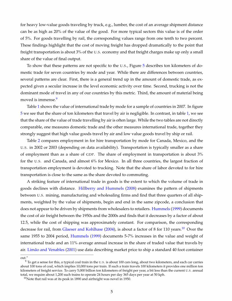
To show that these patterns are not specific to the U.S., Figure 5 describes ton kilometers of do-

mestic trade for seven countries by mode and year. While there are differences between countries,

several patterns are clear. First, there is a general trend up in the amount of domestic trade, as ex-

pected given a secular increase in the level economic activity over time. Second, trucking is not the

dominant mode of travel in any of our countries by this metric. Third, the amount of material being

moved is immense.9

Table 1 shows the value of international trade by mode for a sample of countries in 2007. In figure

5 we see that the share of ton kilometers that travel by air is negligible. In contrast, in table 1, we see

that the share of the value of trade travelling by air is often large. While the two tables are not directly

comparable, one measures domestic trade and the other measures international trade, together they

strongly suggest that high value goods travel by air and low value goods travel by ship or rail.

Table 2 compares employment in for hire transportation by mode for Canada, Mexico, and the

U.S. in 2002 or 2003 (depending on data availability). Transportation is typically smaller as a share

of employment than as a share of GDP. The share of employment in transportation is about 3%

for the U.S. and Canada, and almost 6% for Mexico. In all three countries, the largest fraction of

transportation employment is devoted to trucking. Note that the share of labor devoted to for hire

transportation is close to the same as the share devoted to commuting.

A striking feature of international trade in goods is the extent to which the volume of trade in

goods declines with distance. Hillberry and Hummels (2008) examines the pattern of shipments

between U.S. mining, manufacturing and wholesaling firms and find that three quarters of all ship-

ments, weighted by the value of shipments, begin and end in the same zipcode, a conclusion that

does not appear to be driven by shipments from wholesalers to retailers. Hummels (1999) documents

the cost of air freight between the 1950s and the 2000s and finds that it decreases by a factor of about

12.5, while the cost of shipping was approximately constant. For comparison, the corresponding

decrease for rail, from Glaeser and Kohlhase (2004), is about a factor of 8 for 110 years.10 Over the

same 1955 to 2004 period, Hummels (1999) documents 5-7% increases in the value and weight of

international trade and an 11% average annual increase in the share of traded value that travels by

air. Limao and Venables (2001) use data describing market price to ship a standard 40 foot container

out.”9 To get a sense for this, a typical coal train in the U.S. is about 100 cars long, about two kilometers, and each car carries

about 100 tons of coal, which implies 10,000 tons per train. If such a train travels 100 kilometers it provides one million tonkilometers of freight service. To carry 5,000 billion ton kilometers of freight per year, a bit less than the current U.S. annualtotal, we require about 1,200 such trains to operate 24 hours per day 365 days per year at 50 kph.

10Note that rail was at its peak in 1890 and airfreight was novel in 1950.

5

from Baltimore Maryland to one of about 50 countries around the world in the late 1990s.11 In a

regression of total freight charge on a land-locked country indicator, sea distance and land distance

to destination, they find that the cost to ship a standard container 1,000km by sea is about 190 dollars

while to ship it the same distance over land is about 1,380 dollars. Recalling that a standard con-

tainer can hold about 30 tons, this gives sea rates of about half a cent per ton mile and land rates of

about 5 cents per ton mile, so that overland travel is about 10 times as expensive as sea travel. These

rates seem somewhat low compared to the price of U.S. truck and rail rates reported in Glaeser and

Kohlhase (2004) (28 cents per ton mile for trucks and 3 cents per ton mile for rail). Finally, Clark et al.

(2004) find that the cost of shipping all maritime freight to and from the U.S. is equal to about 5.25%

of the value of freight and that port efficiency is an important contributor to this cost.

These facts paint a subtle picture. While the real costs of moving goods has fallen to astonishingly

low levels and the weight of trade is immense, the fact that not all trade travels by the cheapest mode

and that most trade travels very short distances, suggests the decline in the price per ton of moving

goods is not leading to the ‘death of distance’.

While it is natural to think of time costs as being most important for the movement of people, the

rise of air trade suggests that time in transit is an increasingly important part of the cost of transit

for goods. A back of the envelope calculation bolsters this idea. The capacity of a typical 40 foot

container is about 30 tons. From Duranton et al. (2014), the value per ton of an average U.S. domestic

shipment of electrical appliances is about six thousand dollars per ton. Thus, a typical container

of U.S. electrical appliances can hold about $200,000 worth of freight. From Glaeser and Kohlhase

(2004), shipping this container 1,000 miles by rail will cost about 1, 000× 30× 0.023 = $700. At a 5%

annual rate, daily interest on a million dollar cargo is 200, 000× 0.05/365 = $28, so that on a five day

journey the opportunity cost of travel time is about equal to a fifth of freight charges. An average ton

of manufactures is worth less than a tenth of this, while a typical ton of computer equipment is 15

times as valuable. At least for relatively high value to weight products, time in transit is important.

Moreover, the predominance of short haul trade suggests that, not only are transportation costs

important, but the geography of production is influenced by transportation costs. For example, the

development of 19th century Chicago was heavily influenced by its location relative to its surround-

ing agricultural hinterland, as discussed in Cronon (1991). This points to an important econometric

problem in interpreting the transport costs data presented so far: these data describe equilibrium

transport costs. Therefore, they do not isolate the supply-side production function (or cost func-

tion) for transportation, but are rather influenced by both demand and supply. Although these data

on transport costs are still suggestive, they capture both the cost of transportation (supply) and the

endogenous organization of economic activity in space in response to the cost of transportation (de-

mand). This presents important and difficult econometric problems to which we return below.

Another striking feature of micro data on trade and production is Atalay et al. (2013)’s finding

11To get a sense for the nature of the sample, when the countries are ranked by kilometers of paved road per person,the median country is Kenya. For evidence on the role of containerization in reducing international transport costs, seeBernhofen et al. (2013).

6

that most vertically integrated firms actually ship very little between plants. From the above, we

have the puzzling collection of facts: the cost of moving goods is a small fraction of their value, most

shipments occur over very small distances, most shipments do not travel by the cheapest mode, and

the time cost of freight is probably important. One possible way of rationalizing this combination of

findings is that there is something valuable about proximity other than the reduction in transporta-

tion costs, i.e., agglomeration effects including knowledge spillovers and idea flows. In this case,

trade could decline rapidly with distance even in a world in which transport costs are small, be-

cause most economic activity is clustered together for these other reasons and hence most economic

interactions are over short distances.

Alternatively, one could question whether the idea that transportation costs are really as small as

share of value-added as some of the figures above suggest. Arguably labor used in transportation

should be compared to labor used in production and we should take into account the same kinds of

costs that we think about for commuting, time costs and scheduling costs.

2.2 Household travel and commuting

While the trade literature has typically focused on the movement of goods, another important source

of transport costs in the urban literature is the movement of people. These costs of transporting peo-

ple remain substantial, both in terms of the opportunity cost of time and in terms of a share of overall

household expenditure. Table 3 lists round trip commute times in minutes in a sample of countries

and years for which data was easily available. While we should be concerned that differences in

commute times across countries reflect sampling error and differences in survey methodology, with

this caveat, these data suggest that the country mean round trip commute is about 40 minutes in the

2000-5 window where we have the most observations. These times are fairly closely clustered, with

a standard deviation of just less than eight minutes. If the ‘work day’ consists of eight hours at work

and time in commute, then commuting consumes about 7.5% of labor. Alternatively, if we value time

in commute at half the wage (as is common in the transportation economics literature, see Small and

Verhoef (2007)) and suppose an eight-hour work day, then the value of commute time is about equal

to 3.5% of the value of labor. While this is a large number, it understates the cost of household travel

by restricting attention to commuters and commute trips.

Alternatively, Schafer (2000) summarizes 26 national household travel surveys from countries all

over the world. Averaging across these surveys, again with the caveat about the comparability of

surveys, he finds that daily household travel time is about 73 minutes with a standard deviation of

about 12 minutes. If we value this time at half the wage and again suppose an eight-hour work day,

then the value of time spent in household travel is about 8% of the value of labor. 12 If we take the

12We note that this estimate is problematic for at least two reasons. First, it assigns the time cost of an average workerto an average traveler, when many travellers are likely to have a lower value of time. Second, it assigns the time cost ofan average worker to an average commuter, when wages probably vary systematically with commute distance. With thissaid, on the basis of these surveys, a rough guess would be that the aggregate time cost of household travel is somewherebetween 3.5% and 8% of the aggregate value of labor in an economy.

7

labor share of GDP to be close to the current U.S. level at 0.6, then the time cost of household travel is

between 2.4 and 4.8% of GDP.

Table 4 describes household expenditure shares on transportation for 26 countries and several

years. Again noting the possibility of different methodologies across countries, the mean expen-

diture share is about 16.2% for the 2000-2004 window and about 14.6% for the 2005-9 window with

standard deviations of 5.4 and 3.7%, respectively. Schafer (2000) investigates these shares using older

and somewhat more extensive national accounts data and finds that across countries the average ex-

penditure share for household travel is about 11% with a standard deviation of about 3%. Weighting

household transportation share by 0.6, about the share of expenditure in current U.S. GDP, and

adding time costs, we have that the total costs of household travel are between 9 and 11.4% of GDP.

Two further points are made in Schafer (2000). First, for country level aggregates, per capita

travel time and expenditure share are negatively correlated. Second, for Zambia, only 5% of all trips

are longer than 10km while for the U.S. 5% of trips are longer than 50km. To the extent that these

findings are driven by differences in transportation technologies, they suggest that the transferral of

developed-country transportation technologies to developing countries is likely to lead to substantial

changes in the spatial organization of economic activity.

2.3 External costs

We have so far concerned ourselves with private costs of transportation, time and private expense.

We now turn attention to two costs of transportation that are rarely priced, carbon emissions and

congestion.

Table 5 presents total 2007 Carbon Dioxide Equivalent (CO2e) emissions for the transportation

sector for Canada, Mexico, the U.S. and the UK. Total emissions for the U.S. in 2007 were about

7,000 Megatonnes (Mt), so that the transportation sector accounts for about 30% of U.S. emissions.

To the extent that these costs of transportation are not priced, the market allocation of resources to

the transportation sector will be in general inefficient. With a social cost of about 30$US/ton CO2e,

the social cost of CO2e emissions from transportation in the U.S. is about 21 billion $US/year. This is

only about one tenth of one percent of U.S. GDP. Thus, while greenhouse gas emissions from trans-

portation are important in an absolute sense, they are small relative the total cost of transportation.

Parry et al. (2007) provides a comprehensive survey of the externalities to automobile use, includ-

ing local air pollution, global air pollution, traffic congestion, traffic accidents and other externalities

(such as noise and highway maintenance costs). Couture et al. (2012) estimate that a lower bound on

the deadweight loss from traffic congestion in the U.S. is of the order of 100 bn $US/year, although

we note that these costs are already reflected in transportation expenditure data described above.

8

3 Theoretical Framework

In this section, we outline a multi-region extension of the Helpman (1998) model that follows Red-

ding and Sturm (2008) and Redding (2012). The model incorporates many locations, goods trans-

portation costs within and between locations, and commuting costs within locations. We use the

model to show the effects of improvements in transportation infrastructure on the spatial distribu-

tion of wages, land rents, population and trade within and between locations. Although the model

does not capture all of the theoretical foundations considered in the regional and urban literatures, it

captures many of the standard ingredients, and we use its predictions to structure our review of the

empirical evidence below.13

3.1 Preferences and Endowments

The economy consists of a set of locations indexed by n or i ∈ N, where n will typically refer to a

consuming region and i to a producing region. To refer to a pairwise quantity, such as a distance

or a quantity of trade, we use two subscripts with the first indicating the location of consumption

and the second the location of production. The economy is populated by a mass of representative

consumers, L, who are mobile across locations and are endowed with a single unit of labor that is

supplied inelastically with zero disutility. The effective supply of labor for each location i depends

on its population (Li) and commuting technology (bi), where commuting costs are assumed to take

the iceberg form. For each unit of labor residing in location i, only a fraction bi is available for

production, where 0 < bi < 1 and the remaining fraction 1− bi is lost in commuting. While we treat

bi as a primitive of the model here, it could in principle depend on equilibrium population density

(e.g. if higher population density increases congestion costs).

Preferences are defined over a consumption index of tradeable varieties, Cn, and consumption of

a non-tradeable amenity, Hn, which can be interpreted as housing. For simplicity, we treat the stock

of housing as a primitive of the model, although it could also in principle depend on equilibrium

population density (e.g. if a higher population density increases the supply of housing). The upper

level utility function is assumed to be Cobb-Douglas:14

Un = Cµn H1−µ

n , 0 < µ < 1. (1)

The tradeables consumption index takes the standard constant elasticity of substitution (CES) form:

Cn =

[∑i∈N

Micσ−1

σni

] σσ−1

,

13The model builds on the new economic geography literature synthesized in Fujita et al. (1999). While this literatureassumes firm product differentiation and monopolistic competition, the model shares many properties with perfectly com-petitive models such as Eaton and Kortum (2002) (see Redding (2012)) or the Armington model of product differentiationby location (see Allen and Arkolakis (2013)). The organization of economic activity within countries has recently receivedrenewed attention, as in Cosar and Fajgelbaum (2013) and Ramondo et al. (2012).

14For empirical evidence using U.S. data in support of the constant housing expenditure share implied by the Cobb-Douglas functional form, see Davis and Ortalo-Magne (2011).

9

where σ is the elasticity of substitution between varieties and we assume that varieties are substitutes

(σ > 1); cni denotes consumption in country n of a variety produced in country i; we have used the

fact that the measure of varieties Mi produced in location i are consumed in location n in the same

amount cni. Varieties are assumed to be subject to iceberg trade costs. In order for one unit of a

variety produced in location i to arrive in location n, a quantity dni > 1 must be shipped, so that

dni − 1 measures proportional trade costs. The price index dual to the tradeables consumption index

Cn is given by:

Pn =

[∑i∈N

Mi p1−σni

]1/(1−σ)

, (2)

where we have used the fact that the measure Mi of varieties produced in location i face the same

elasticity of demand and charge the same equilibrium price pni = dni pi to consumers in location n.

Applying Shephard’s lemma to the tradeables price index, equilibrium demand in location n for

a tradeable variety produced in i is:

xni = p−σi (dni)

1−σ (µvnLn) (Pn)σ−1 , (3)

where vnLn denotes total income which equals total expenditure and, with Cobb-Douglas utility,

consumers spend a constant share of their income, µ, on tradeables.

With constant expenditure shares and an inelastic supply of the non-tradeable amenity, the equi-

librium price of this amenity depends solely on the expenditure share, (1− µ), total income, vnLn,

and the supply of the non-tradeable amenity, Hn:

rn =(1− µ)vnLn

Hn. (4)

Total income is the sum of labor income and expenditure on the non-tradeable amenity, which is

assumed to be redistributed lump-sum to the location’s residents:

vnLn = wnbnLn + (1− µ)vnLn =wnbnLn

µ, (5)

where we have used the fact that only a fraction bn of the labor in location i is used in production

because of commuting costs. Therefore total labor income equals the wage per effective unit of labor

(wn) times the measure of effective units of labor (bnLn).

3.2 Production Technology

There is a fixed cost in terms of labor of producing tradeable varieties (F > 0) and a constant variable

cost that depends on a location’s productivity (Ai). Both the fixed cost and the variable cost are

the same across all varieties produced within a location. The total amount of labor (li) required to

produce xi units of a variety in location i is:

li = F +xi

Ai, (6)

10

where we allow productivity (Ai) to vary across locations to capture variation in production funda-

mentals.

Profit maximization implies that equilibrium prices are a constant markup over marginal cost:

pni =

(σ

σ− 1

)dniwi

Ai. (7)

Combining profit maximization and zero profits, equilibrium output of each tradeable variety equals

the following constant:

x = xi = ∑n

xni = AiF(σ− 1). (8)

Labor market clearing for each location implies that labor demand equals the effective labor sup-

ply in that location, which is in turn determined by population mobility. Using the constant equi-

librium output of each variety (8) and the tradeables production technology (6), the labor market

clearing condition can be written as follows:

biLi = Mili = MiFσ, (9)

where li denotes the constant equilibrium labor demand for each variety. This relationship pins

down the measure of tradeable varieties produced in each location as a function of the location’s

population, the commuting technology, and the parameters of the model.

3.3 Market Access and Wages

Given demand in all markets and trade costs, the free on board price (pi) charged for a tradeable va-

riety by a firm in each location must be low enough in order to sell the quantity x and cover the firm’s

fixed production costs. We saw above that prices are a constant mark-up over marginal cost. There-

fore, given demand in all markets, the equilibrium wage in location i, wi, must be sufficiently low in

order for a firm to sell x and cover its fixed production costs. Using demand (3), profit maximization

(7) and equilibrium output (8), we obtain the tradeables wage equation:(σ

σ− 1wi

Ai

)σ

=1x ∑

n∈N(wnbnLn) (Pn)

σ−1 (dni)1−σ . (10)

This relationship pins down the maximum wage that a firm in location i can afford to pay given

demand in all markets, trade costs and the production technology. On the right-hand side of the

equation, market n demand for tradeables produced in i depends on total expenditure on tradeable

varieties, µvnLn = wnbnLn, the tradeables price index, Pn, that summarizes the price of competing

varieties, and on bilateral trade costs, dni. Total demand for tradeables produced in i is the weighted

sum of demand in all markets, where the weights are these bilateral trade costs, dni.

Following Redding and Venables (2004), we define the weighted sum of market demands faced

by firms as firm market access, f mai, such that the tradeables wage equation can be written more

compactly as:

wi = ξAσ−1

σi [ f mai]

1/σ , f mai ≡ ∑n∈N

(wnbnLn) (Pn)σ−1 (dni)

1−σ , (11)

11

where ξ ≡ (F (σ− 1))−1/σ (σ− 1) /σ collects together earlier constants. Therefore wages are increas-

ing in both productivity Ai and firm market access ( f mai). Investments in transportation infrastruc-

ture that reduce the costs of transporting goods (dni) to market demands ((wnbnLn) (Pn)σ−1) raise

market access and wages. Improvements in the commuting technology (bn) increase the effective

supply of labor (bnLn) and hence total income, which also raises market access and wages.

3.4 Labor Market Equilibrium

With perfect population mobility, workers move across locations to arbitrage away real income differ-

ences. Real income in each location depends on per capita income (vn), the price index for tradeables

(Pn), and the price of the non-tradeable amenity (rn). Therefore population mobility implies:

Vn =vn

(Pn)µ (rn)

1−µ= V, (12)

for all locations that are populated in equilibrium, where we have collected the constants µ−µ and

(1− µ)−(1−µ) into the definition of Vn and V.

The price index (2) that enters the above expression for real income depends on consumers’ access

to tradeable varieties, as captured by the measure of varieties and their free on board prices in each

location i, together with the trade costs of shipping the varieties from locations i to n. We summarize

consumers’ access to tradeables using the concept of consumer market access, cman:

Pn = [cman]1/(1−σ) , cman ≡ ∑

i∈NMi(pidni)

1−σ. (13)

Substituting for vn, Pn and rn, the labor mobility condition (12) can be re-written to yield an ex-

pression linking the equilibrium population of a location (Ln) to its productivity (An), its commuting

technology (bn), the supply of the non-traded amenity (Hn), and the two endogenous measures of

market access introduced above (one for firms ( f man) and one for consumers (cman)):

Ln = χbµ

1−µn A

µ(σ−1)σ(1−µ)n Hn( f man)

µσ(1−µ) (cman)

µ(1−µ)(σ−1) , (14)

where χ = V−1/(1−µ)ξµ/(1−µ)µ−µ/(1−µ) (1− µ)−1 is a function of the common real income V.

Therefore equilibrium population (Ln) is increasing in the quality of the commuting technology

(bn), the productivity of the final goods production technology (An), and the supply of the non-

traded amenity (Hn). Investments in transportation infrastructure that reduce the costs of transport-

ing goods (dni) raise both firm and consumer market access ( f man and cman) and hence increase

equilibrium population. Improvements in the commuting technology (bn) also have positive indirect

effects on equilibrium population through higher firm and consumer market access.

From land market clearing (4) and total labor income (5), land prices can be written in terms of

wages and total population:

rn =(1− µ)

µ

wnbnLn

Hn. (15)

12

Therefore higher firm market access raises ( f man) land prices through both higher wages (from (10))

and higher population (from (14)), while higher consumer market access (cman) raises land prices

through a higher population alone (from (14)). Reductions in the cost of transporting goods (dni) raise

land prices through both firm and consumer market access. Improvements in commuting technology

(bn) raise land prices directly and also indirectly through higher wages and population.

3.5 Trade Flows

Using CES demand, the share of location n’s expenditure on varieties produced by location i can be

expressed as:

πni =Mi p1−σ

ni

∑k∈N Mk p1−σnk

, (16)

which, using the equilibrium pricing rule (7) and the labor market clearing condition for each location

(9), can be written as:

πni =biLi (dniwi)

1−σ (Ai)σ−1

∑k∈N bkLk (dnkwk)1−σ (Ak)

σ−1 . (17)

This expression for bilateral trade shares (πni) corresponds to a “gravity equation,” in which bilateral

trade between exporter i and importer n depends on both “bilateral resistance” (i.e. the bilateral

goods of trading goods between i and n (dni) in the numerator) and “multilateral resistance” (i.e. the

bilateral costs for importer n of sourcing goods from all exporters k (dnk) in the denominator). In this

gravity equation specification, bilateral trade depends on characteristics of the exporter i (e.g. the

exporter’s wage wi in the numerator), bilateral trade costs (dni), and characteristics of the importer n

(i.e. the importer’s access to all sources of supply in the denominator).15

Taking the ratio of these expenditure shares, the value of trade between locations (Xni) relative to

trade within locations (Xnn) is:

Xni

Xnn=

πni

πnn=

biLi (dniwi)1−σ (Ai)

σ−1

bnLn (dnnwn)1−σ (An)

σ−1 . (18)

Therefore transportation infrastructure improvements that reduce the cost of transporting goods

within locations (dnn) by the same proportion as they reduce the cost of transporting goods between

locations (dni) leave the ratio of trade between locations to trade within locations unchanged. One

potential example is building roads within cities that make it easier for goods to circulate within the

city and to leave the city to connect with long distance highways. Transportation cost improvements

that reduce commuting costs for all locations (increase bn and bi) also leave the ratio of trade between

locations to trade within locations unchanged.

In this model with a single differentiated sector, all trade takes the form of intra-industry trade,

and transport infrastructure improvements affect the volume of this intra-industry trade. More gen-

erally, in a setting with multiple differentiated sectors that differ in terms of the magnitude of trade

15For an insightful review of the gravity equation in the international trade literature, see Head and Mayer (2013).

13

costs (e.g. high value to weight versus low value to weight sectors), transport infrastructure im-

provements also affect the pattern of inter-industry trade and the composition of employment and

production across sectors within locations.

3.6 Welfare

We now show how the structure of the model can be used to derive an expression for the welfare

effects of transport infrastructure improvements in terms of observables. Using the trade share (16),

the price index (2) can be re-written in terms of each location’s trade share with itself and parameters:

Pn =σ

σ− 1

(bnLn

σFπnn

) 11−σ dnnwn

An. (19)

Using this expression for the price index and land market clearing (15), the population mobility

condition (12) implies that the equilibrium population for each location can be written as:

Ln =

(

1σFπnn

) µσ−1 H1−µ

n bµσ

σ−1n Aµ

n

µ(

1−µµ

)1−µ (σ

σ−1

)µ Vdµnn

,

σ−1

σ(1−µ)−1

. (20)

where terms in wages (wn) have canceled and labor market clearing for the economy as a whole

implies:

∑n∈N

Ln = L. (21)

This expression for equilibrium population (20) has an intuitive interpretation. The population of

each location n is decreasing in its domestic trade share (πnn), since locations with low domestic

trade shares have good market access to sources of supply of tradables from other locations. The

population of each location is also increasing in the efficiency of its commuting technology (bn), its

productivity in production (An), its supply of housing (Hn), and the efficiency of its transport tech-

nology (inversely related to dnn). The common level of utility across all locations (V) is endogenous

and determined by the requirement that the labor market clears for the economy as a whole.

Re-arranging the population mobility condition (20), the real income in each location can be writ-

ten in terms of its population, trade share with itself and parameters.

Vn =

(1

σFπnn

) µσ−1 L

−(

σ(1−µ)−1σ−1

)n H1−µ

n bµσ

σ−1n Aµ

n

µ(

1−µµ

)1−µ (σ

σ−1

)µ dµnn

= V. (22)

A key implication of this expression for real income is that the change in each location’s trade

share with itself and the change in its population are sufficient statistics for the welfare effects of

improvements in transport technology that reduce the costs of trading goods (see Redding, 2012):

V1n

V0n=

(π0

nnπ1

nn

) µσ−1(

L0n

L1n

)( σ(1−µ)−1σ−1

)=

V1

V0 , (23)

14

where the superscripts 0 and 1 denote the value of variables before and after the improvement in

transport technology respectively.

Similar sufficient statistics apply for the welfare effects of improvements in transport technology

that reduce commuting costs, although these welfare effects also depend directly on the change in

commuting costs (though the resulting increase in the effective supply of labor):

V1n

V0n=

(b1

nb0

n

) µσσ−1(

π0nn

π1nn

) µσ−1(

L0n

L1n

)( σ(1−µ)−1σ−1

)=

V1

V0 . (24)

While these improvements in transport infrastructure have uneven effects on wages, land prices,

and population, the mobility of workers across locations ensures that they have the same effect on

welfare across all populated locations.

To understand the relationship between changes in domestic trade shares and the welfare change

from improvements in transport technology that reduce goods trade costs, consider the extreme case

where the transport improvement allows goods trade between two previously autarkic locations.

For locations closed to goods trade, domestic trade shares must equal to one. Once locations open to

trade, they can specialize to exploit gains from trade with other locations, and domestic trade shares

fall below one. This fall in the domestic trade shares reflects the increase in specialization and is

directly related to increases in real income, our measure of welfare.

To understand the relationship between changes in population and the changes in welfare fol-

lowing improvements in transport technology that reduce goods trade costs, first note that labor mo-

bility requires real wage equalization across populated locations. Therefore, if goods trade is opened

between locations, and some locations (e.g. coastal regions) benefit more than other locations (e.g.

interior regions) at the initial labor allocation, workers must relocate to arbitrage away real wage

differences. Those locations that experience larger welfare gains from trade at the initial labor allo-

cation will experience population inflows, which increases the demand for the immobile factor land,

and bids up land prices. In contrast, those locations that experience smaller welfare gains from trade

at the initial labor allocation will experience population outflows, which decreases the demand for

land, and bids down land prices. This population reallocation continues until real wages are again

equalized across all populated locations. Hence these population changes also need to be taken into

account in computing the welfare effects of the improvement in transport technology.

Therefore, together, the change in a location’s domestic trade share and its population are suffi-

cient statistics for the effects of a transport improvement that reduces the costs of trading goods (dni).

A transport improvement that reduces the commuting costs for a region (bn) also directly increases

the supply of labor for that region, which is taken into account in the welfare formula.

3.7 General Equilibrium

The general equilibrium of the model can be represented by the share of workers in each location

(λn = Ln/L), the share of each location’s expenditure on goods produced by other locations (πni)

15

and the wage in each location (wn). Using labor income (5), the trade share (16), population mobility

(20) and labor market clearing (21), the equilibrium triple {λn, πni, wn} solves the following system

of equations for all i, n ∈ N (see Redding, 2012):

wibiλi = ∑n∈N

πniwnbnλn, (25)

πni =biλi (dniwi/Ai)

1−σ

∑k∈N bkλk (dnkwk/Ak)1−σ

, (26)

λn =

[H1−µ

n

(1

πnn

) µσ−1 b

µσσ−1n Aµ

nd−µnn

] σ−1σ(1−µ)−1

∑k∈N

[H1−µ

k

(1

πkk

) µσ−1 b

µσσ−1k Aµ

k d−µkk

] σ−1σ(1−µ)−1

. (27)

The assumption that σ(1− µ) > 1 corresponds to the “no black hole” condition in Krugman (1991)

and Helpman (1998). For parameter values satisfying this inequality, the model’s agglomeration

forces from love of variety, increasing returns to scale and transport costs (which are inversely related

to σ) are not too strong relative to its congestion forces from an inelastic supply of land (captured by

1− µ). As a result, each location’s real income is monotonically decreasing in its population, which

ensures the existence of a unique stable non-degenerate distribution of population across locations.

While the existence of a unique equilibrium ensures that the model remains tractable and amenable

to counterfactual analysis, often the rationale for transport investments is cast in terms of shifting the

distribution of economic activity between multiple equilibria. To the extent that such multiple equi-

libria exist, their analysis requires either consideration of the range of the parameter space for which

the model has multiple equilibria or the use of a richer theoretical framework.16

3.8 Counterfactuals

The system of equations for general equilibrium (25)-(27) can be used to undertake model-based

counterfactuals in an extension of the trade-based approach of Dekle et al. (2007) to incorporate factor

mobility across locations. The system of equations for general equilibrium must hold both before

and after any counterfactual change in for example transport infrastructure. Denote the value of

variables in the counterfactual equilibrium with a prime (x′) and the relative value of variables in the

counterfactual and initial equilibria by a hat (x = x′/x). Using this notation, the system of equations

for the counterfactual equilibrium (25)-(27) can be re-written as follows:

wi biλiYi = ∑n∈N

πniπniwnbnλnYn, (28)

16An empirical literature has examined whether large and temporary shocks have permanent effects on the location ofeconomic activity and interpreted these permanent effects as either evidence of multiple equilibria or path dependencemore broadly. See for example Bleakley and Lin (2012), Davis and Weinstein (2002), Maystadt and Duranton (2014),Redding et al. (2011) and Sarvimaki et al. (2010).

16

πniπni =πniλi bi

(dniwi/Ai

)1−σ

∑k∈N πnkλi bi

(dnkwk/Ai

)1−σ, (29)

λnλn =

λn

[ˆH1−µπ

− µσ−1

nn bµσ

σ−1n Aµ

n d−µnn

] σ−1σ(1−µ)−1

∑k∈N λk

[ˆH1−µ

k π− µ

σ−1kk b

µσσ−1k Aµ

k d−µkk

] σ−1σ(1−µ)−1

, (30)

where Yi = wibiLi denotes labor income in the initial equilibrium.

Given an exogenous change in transportation infrastructure that affects the costs of trading goods

(dni) or the costs of commuting (bn), this system of equations (28)-(30) can be solved for the coun-

terfactual changes in wages (wn), population shares (λn) and trade shares (πni). Implementing

these counterfactuals requires only observed values of GDP, trade shares and population shares

{Yn, πni, λn} for all locations i, n ∈ N in the initial equilibrium. For parameter values for which

the model has a unique stable equilibrium (σ(1− µ) > 1), these counterfactuals yield determinate

predictions for the impact of the change in transportation costs. From the welfare analysis above,

the changes in each location’s population and its domestic trade share provide sufficient statistics for

the welfare effect of transport improvements that affect the costs of trading goods (dni). In contrast,

transport improvements that affect the costs of commuting (bn) also have direct effects on welfare

in addition to their effects through population and domestic trade shares. With perfect population

mobility, these welfare effects must be the same across all populated locations.

4 Reduced-form Econometric Framework

4.1 A simple taxonomy

We survey the recent empirical literature investigating the effects of infrastructure on the geographic

distribution of economic activity. The preponderance of this literature can be described with a re-

markably simple taxonomy.

Let t index time periods, and, preserving the notation from above, let n and i ∈ N index a set of

geographic locations, typically cities or counties. Let Lit denote an outcome of interest for location

i at time t; employment, population, rent or centralization. Let xit be a vector of location and time

specific covariates, and finally, let bit and dit denote the transportation variables of interest. In par-

ticular, consistent with notation in our theoretical model, let bit denote a measure of transportation

infrastructure that is internal to unit i, and dit a measure of transportation infrastructure external

to unit i. For example, bit could count radial highways within a metropolitan area while dit could

indicate whether a rural county is connected to a highway network.

With this notation in place, define the ‘intracity regression’ as

Lit = C0 + C1bit + C2xit + δi + θt + εit, (31)

17

where δi denotes location specific time invariant unobservables, θt a common time effect for all lo-

cations and εit the time varying location specific residual. The coefficient of interest is C1, which

measures the effect of within-city infrastructure on the city level outcome.17

Similarly, define the ‘intercity regression’ as

Lit = C0 + C1dit + C2xit + δi + θt + εit, (32)

which differs from the intracity regression only in that the explanatory variable of interest describes

transportation costs between unit i and other units, rather than within-city infrastructure.

These equations require some discussion before we turn to a description of results. First, both

estimating equations are natural reduced form versions of equation (14), or if the outcome of inter-

est is land rent, (15). Thus, they are broadly consistent with the theoretical framework described

earlier. Second, comparing the regression equations with their theoretical counterparts immediately

suggests four inference problems that estimations of the intracity and intercity regressions should

confront.

First, equilibrium employment or land rent depends on the location specific productivity, An.

This will generally be unobserved, and thus will be reflected in the error terms of our regression

equations. It is natural to expect that intracity and intercity infrastructure will depend on location

specific productivity, and hence, be endogenous in the two regression equations. Second, equilibrium

employment or land rent depends on the level of a location specific amenity, Hn. In our model, this

reflects a supply of housing, but in reality, may also reflect unobserved location characteristics that

augment or reduce the welfare of residents at a location. We might also be concerned that such

amenities, to the extent that they are unobserved, affect infrastructure allocation and give rise to an

endogeneity problem. More generally, the intercity and intracity regressions do not by themselves

distinguish between the demand for and supply of transportation.

Third, equations (14) and (15) involve expressions for market access not present explicitly in the

estimating equations. To the extent that market access depends on transportation costs between

cities, the treatment of market access in these estimations deserves careful attention. Fourth, to the

extent that there are general equilibrium effects of transport infrastructure on all locations, these

are not captured by C1. Instead they are captured in the time effects θt and cannot be separated

from other time-varying factors that are common to all locations without further assumptions. More

generally, in general equilibrium, transport investments between a pair of regions i and j can have

effects on third regions k, which are not captured by the transportation variables for regions i and j.

4.2 Identification of causal effects

As discussed above, perhaps the biggest empirical challenge in estimating the intercity and intracity

regressions is constructing the appropriate counterfactual for the absence of the transport improve-

17Pioneering studies of the role of automobiles and highways in reorganizing the distributions of population and eco-nomic activity within metropolitan areas are Moses (1958) and Moses and Williamson (1963).

18

ment. In particular, ordinary least squares (OLS) regressions comparing treated and untreated lo-

cations are unlikely to consistently estimate the causal effect of the transport improvement, because

the selection of locations into the treatment group is non-random. The main empirical approach

to addressing this challenge has been to develop instruments for the assignment of transport im-

provements that plausibly satisfy the exclusion restriction of only affecting the economic outcome

of interest through the transport improvement.18 More formally, this approach to identifying the

causal effects posits an additional first-stage regression that determines the assignment of transport

infrastructure:

Iit = D0 + D1xit + D2zit + ηi + γt + uit, (33)

where Iit ∈ {bit, dit} is the transportation variables of interest (depending on whether the specifi-

cation is intracity or intercity); xit are the location and time-varying controls from the second-stage

regression ((31) or (32)); ηi are location specific time invariant unobservables; γt are time indicators;

uit is a time varying location specific residual; and zit are the instruments or excluded exogenous

variables.

Combining the second-stage equation ((31) or (32)) with the first-stage equation (33), the impact

of transport infrastructure on the economic outcomes of interest (C1) can be estimated using two-

stage least squares. Credible identification of the causal impact of transport infrastructure requires

that two conditions are satisfied: (i) the instruments have power in the first-stage regression (D2 6= 0)

and (ii) the instruments satisfy the exclusion restriction of only affecting the economic outcomes of

interest through transport infrastructure conditional on the controls xit, that is, cov(εit, uit) = 0.

The existing literature has followed three main instrumental variables strategies. The first, the

planned route IV, is an instrumental variables strategy which relies on planning maps and documents

as a source of quasi-random variation in the observed infrastructure. The second, the historical route

IV, relies on very old transportation routes as a source of quasi-random variation in observed in-

frastructure. The third, the inconsequential place approach, relies on choosing a sample that is incon-

sequential in the sense that unobservable attributes do not affect the placement of infrastructure.

The plausibility of these identification strategies depends sensitively on the details of their imple-

mentation and is sometimes contentious. With this said, we here briefly describe these identification

strategies and the rationale for their use. We avoid discussion of the validity of these strategies in

particular contexts. Broadly, the strategies we describe are the best approaches currently available

for estimating the causal effects of transport infrastructure on the organization of economic activity.

4.2.1 Planned Route IV

Baum-Snow (2007) pioneers the planned route IV by using a circa 1947 plan for the interstate high-

way network as a source of quasi-random variation in the way the actual network was developed.

18While the program evaluation literature suggests other complementary approaches, such as conducting randomizedexperiments with transport improvements or the use of matching estimators, these have been less widely applied in thisempirical literature.

19

In the specific context of Baum-Snow (2007), this means counting the number of planned radial high-

ways entering a metropolitan area and using this variable to predict the actual number of interstate

highway rays. Since the network plan was developed under a mandate to serve military purposes,

the validity of this instrument hinges on the extent to which military purposes are orthogonal to the

needs of post war commuters. Several other empirical investigations into the effects of the U.S. road

and highway network exploit instruments based on the 1947 highway plan, while Hsu and Zhang

(2012) develop a similar instrument for Japan. Michaels et al. (2012) uses an even earlier plan of the

U.S. highway network, the ‘Pershing plan’, as a source of quasi-random variation in the U.S. high-

way network. Although Donaldson (2013) stops short of using hypothetical planned networks as

instruments for realized networks, he does compare the development of districts without railroads

and without planned railroads to those without railroads but with planned railroads. That these sets

of districts develop in the same way suggests that the planning process did not pick out districts on

the basis of different unobservable characteristics.

4.2.2 Historical Route IV

Duranton and Turner (2012) develop the historical route IV approach. In regressions predicting MSA

level economic outcomes they rely on maps of historical transportation networks, the U.S. railroad

network circa 1898 and the routes of major expeditions of exploration of the U.S. between 1535 and

1850 as sources of quasi-random variation in the U.S. interstate highway network at the end of the

20th century. The validity of these instruments requires that, conditional on controls, factors that do

not directly affect economic activity in U.S. metropolitan areas at the end of the 20th century deter-

mine the configuration of these historical networks. A series of papers, Duranton and Turner (2011),

Duranton and Turner (2012) and Duranton et al. (2014), use the two historical route instruments and

the 1947 highway plan as sources of quasi-random variation in regressions predicting metropolitan

total vehicle kilometers traveled, changes in metropolitan employment, and trade flows between

cities as functions of the interstate highway network.

One distinctive feature of Duranton and Turner (2011), Duranton and Turner (2012), and Du-

ranton et al. (2014) is the use of multiple instruments based on different sources of variation. With

more instruments than endogenous variables, the specification can be estimated with either all or

subsets to the instruments, and over-identification tests can be used as a check on the identifying

assumptions. Conditional on one of the instruments being valid, these over identification tests check

the validity of the other instruments. Given that the instruments exploit quite different sources of

variation in the data, if a specification passes the over-identification test, this implies that either all of

the instruments are valid or that an improbable relationship exists between the instruments and the

errors of the first and second-stage regressions.

Several other authors develop historical transportation networks as a source of quasi-random

variation in modern transportation networks in other regions. Baum-Snow et al. (2012) rely on Chi-

nese road and rail networks from 1962 as a source of quasi-random variation in road and rail net-

20

works after 2000. Garcia-Lopez et al. (2013) use 18th century postal routes and Roman roads for

Spain. Hsu and Zhang (2012) relies on historical Japanese railroad networks. Martincus et al. (2012)

uses the Inca roads for Peru. Duranton and Turner (2012) provides a more detailed discussion of the

validity of these instruments.

4.2.3 Inconsequential Units Approach

To estimate the intercity regression, researchers often rely on the inconsequential units approach to

identification, sometimes in conjunction with one or both of the instrumental variables strategies de-

scribed above. If we consider economically small units lying between large cities, then we expect

that intercity links will traverse these units only when they lie along a convenient route between the

two large cities. That is, we expect that the unobserved characteristics of units between large cities

are inconsequential to the choice of route, and therefore that the connection status of these units will

not depend on the extent to which these units are affected by the road. Chandra and Thompson

(2000) pioneer this strategy in their analysis of the effect of access to the interstate highway system

on rural counties in the U.S.. By restricting attention to rural highways they hope to restrict attention

to counties that received interstates ‘accidentally’, by virtue of lying between larger cities. While it is

difficult to assess the validity of this approach, some of the regressions reported in Michaels (2008)

are quite similar to those in Chandra and Thompson (2000) but rely on the 1947 planned highway

network for identification. That the two methods arrive at similar estimates is reassuring. Banerjee

et al. (2012) also use the inconsequential units strategy in their analysis of the effects of Chinese trans-

portation networks. In particular, they construct a hypothetical transportation network connecting

historical treaty ports to major interior trading centers. Counties near these predicted networks are

there accidentally in the same sense that rural counties may be accidentally near interstates in the

U.S. Similarly, and also for China, Faber (2014) constructs a hypothetical least cost network con-

necting major Chinese cities and examines the impact of proximity to this network on outcomes in

nearby rural counties.

These three econometric responses to the probable endogeneity of transportation infrastructure

are widely used. Other approaches to this problem typically exploit natural experiments that, while

they may provide credible quasi-random variation in infrastructure, are not easily extended to other

applications.

4.3 Distinguishing growth from reorganization

As Fogel observes in his classic analysis of the role of railroad construction in the economic devel-

opment of the 19th century U.S. (Fogel, 1964), an assessment of the economic impacts of transporta-

tion infrastructure depends fundamentally on whether changes in transportation costs change the

amount of economic activity or reorganize existing economic activity. For example, the welfare im-

plications of a road or light rail line that attracts pre-existing firms are quite different than those of

one that leads to the creation of new firms. Importantly, this issue is distinct from the endogene-

21

ity problem discussed above. The problem of endogeneity follows from non-random assignment

of transportation infrastructure to ‘treated’ observations. The problem of distinguishing between

growth and reorganization persists even when transportation is assigned to observations at random.

Even in the case in which a region experiences an exogenous change in transport infrastructure, the

observed effects on economic activity in the region can either reflect reorganization or growth. This

same issue of distinguishing growth and reorganization appears in the literature evaluating place-

based policies, as discussed in Neumark and Simpson (2014) in this volume.19

Figure 6 illustrates a simple hypothetical data set with the same structure as those typically used

to estimate the intercity and intracity estimating equations. Figure 6 describes a sample consisting

of three regions: a region that is ‘treated’ in some way that affects transportation costs in this region,

e.g., a new road; an untreated region which is typically near the treated region but is not subject to a

change in transportation infrastructure; and third, everyplace else. The outcome variable of interest

is y and the new road creates a units of this outcome in the treated region and displaces d units from

the untreated to the treated region.

Fundamentally, the intercity and intracity regressions estimate the effect of treatment on the dif-

ference between treated regions and untreated comparison regions. As the figure makes clear, the

difference in the outcome between treated and untreated regions is 2d + a, the compound effect of

reorganization and growth. At its core, the problem of distinguishing between reorganization and

growth requires us to identify two quantities. Without further assumptions, these two quantities

cannot be separately identified if we estimate only a single equation, regardless of whether it is the

intercity or intracity estimating equation. To identify both the growth and reorganization effect, we

must estimate two linearly independent equations.

In the context of the sample described in figure 6 these two equations could involve a comparison

of any two of the three possible pairs of regions, i.e., treated and untreated, untreated and residual,

treated and residual. Alternatively, with panel data, one could estimate the change in the treated

region following a change in transportation costs and also the change in the untreated region follow-

ing the change in the treated region. While the literature has carefully addressed the possibility that

transportation costs and infrastructure are not assigned to regions at random, few authors conduct

estimations allowing the separate identification of growth and reorganization.

While figure 6 suggests simple methods for distinguishing between growth and reorganization,

this reflects implicit simplifying assumptions. In particular, the new road in the treated district does

not lead to migration of economic activity from the residual to the untreated or the treated region and

does not cause growth in the untreated or residual district. If we allow these effects, then the effect

of a new road in the treated region is characterized by six parameters rather than two. Identifying all

of these parameters will generally require estimating six linearly independent equations and will not

generally be possible with cross-sectional data. In the context of ‘real data’, with a more complex ge-

19For approaches to distinguishing growth and reorganization in this literature on place-based policies, see Criscuoloet al. (2012) and Thierry Mayer and Py (2013).

22

ography and many regions subject to treatment, distinguishing between growth and reorganization

requires a priori restrictions on the nature of these effects.

The literature has, as yet, devoted little attention to what these identifying assumptions should

be. As suggested by figure 6, this problem can be resolved with transparent but ad hoc assumptions.

Alternatively, the theoretical model described in section 3 provides a theoretically founded basis for

distinguishing between growth and reorganization which derives from the iceberg structure of trans-

portation costs and increasing returns to scale in cities. Importantly, if the new road in the treated

region affects the level of economic activity in all three regions, then no cross-sectional estimate can

recover this effect. This requires time series data or cross-sectional data describing ‘replications’ of

figure 6. More generally, for a penetration road or single transport project, it may be possible to con-

struct plausible definitions of treated, untreated and residual regions, as in Figure 6. However, for an

evaluation of a national highway system, there may be no plausible residual regions, in which case

we are necessarily in a general equilibrium world.

5 Reduced-form empirical results

5.1 Intracity infrastructure and the geographic organization of economic activity

5.1.1 Infrastructure and decentralization

Baum-Snow (2007) partitions a sample of U.S. metropolitan areas into an ‘old central business dis-

trict’, the central business district circa 1950, and the residual suburbs. He then estimates a version

of the intracity regression, equation (31), in first differences, where the unit of observation is a U.S.

MSA, the measure of infrastructure is the count of radial interstate highways, and the instrument is a

measure of rays based on the 1947 highway plan discussed above. He finds that each radial segment

of the interstate highway network causes about a 9% decrease in central city population. Since one

standard deviation in the number of rays in an MSA is 1.5, this means that a one standard deviation

increase in the number of rays causes about a 14% decrease in central city population. To get a sense

for the magnitude of this effect, U.S. population grew by 64% during his study period, MSA popu-

lation by 72% and constant boundary central city population declined by 17%. Thus, the interstate

highway system can account for almost the entire decline in old central city population densities.

Note that, since Baum-Snow (2007) estimates the share of population in the treated area, he avoids

the problem of distinguishing between growth and reorganization. The share of population in the

central city reflects changes in the level of central city and suburb and migration between the two.

This result has been extended to two other contexts. Baum-Snow et al. (2012) conduct essentially

the same regression using data describing Chinese prefectures between 1990 and 2010. They first

partition each prefecture into the constant boundary administrative central city and the residual

prefecture, and then examine the effect of several measures of infrastructure on the decentralization

of population and employment. They rely on a historical routes (from 1962) as a source of quasi-

random variation in city level infrastructure. They find that each major highway ray causes about a

23

5% decrease in central city population. No other measure of infrastructure; kilometers of highways,

ring road capacity, kilometers of railroads, ring rail capacity or radial rail capacity, has a measurable

effect on the organization of population in Chinese prefectures. Baum-Snow et al. (2012) also examine

the effect of infrastructure on the organization of production. They find that radial railroads and

highway ring capacity both have dramatic effects on the organization of production. In particular,

each radial railroad causes about 26% of central city manufacturing to migrate to the periphery while

ring roads also have a dramatic effect. This effect varies by industry. Industries with relatively low

weight to value ratios are more affected. None of the other infrastructure measures they investigate

affect the organization of production.

Finally, Garcia-Lopez et al. (2013) consider the effect of limited access highways on the organiza-

tion of population in Spanish cities between 1991 and 2011. Their unit of observation is one of 123

Spanish metropolitan regions. They conduct a version of the intracity regression in first differences

to explain the change in central city population between 1991 and 2011 as a function of changes in the

highway network over the same period. They rely on three historical road networks to instrument

for changes in the modern network: the Roman road network; a network of postal roads, circa 1760;

and a network of 19th century main roads. They find that each radial highway causes about a 5%

decrease in central city population, and that kilometers of central city or suburban highways have no

measurable effect. Using a similar instrumentation strategy, Angel Garcia-Lopez (2012) examines the

impact of transport improvements on the location of population within the city of Barcelona. Consis-

tent with some of the findings discussed above, improvements to the highway and railroad systems

are found to foster population growth in suburban areas, whereas the expansion of the transit system

is found to affect the location of population inside the central business district (CBD).20

Where the decentralization papers above investigate the effect on central cities of infrastructure

improvements which reduce the cost of accessing peripheral land, the Ahlfeldt et al. (2012) consid-

ers the effect of changes in transportation cost between two adjacent parts of the same central city.

Specifically, Ahlfeldt et al. (2012) consider the effect of the construction and destruction of the Berlin

wall, which bisected the historical central business district, on the organization of population, em-

ployment and land values in 1936, before the partition of the city, 1986, shortly before reunification,

and 2006, 15 years after reunification. That is, when the cost of commuting from the West to the East

was, low, prohibitively high, and low again.

Methodologically, Ahlfeldt et al. (2012) differs dramatically from the centralization papers above.

Their sample consists of approximately 16,000 ‘statistical blocks’ comprising metropolitan Berlin,

each with a population of about 250 people in 2005. Loosely, for each block, Ahlfeldt et al. (2012)

record location, population, land rent and employment in the three years of their study. They use

these data to estimate a first differences variant of the intercity regression, equation (32). The reduced

form results in Ahlfeldt et al. (2012) show that the construction of the Berlin Wall caused the central

20One issue that has received relatively little attention in the intracity literature is the role of transport infrastructure insegregating cities and leaving some neighborhoods “on the wrong side of the tracks.”

24

business district to migrate so that it was more nearly central in the territory of West Berlin, and

that the removal of the Berlin Wall approximately reversed this process. The identifying assumption

underlying this natural experiment is that change in access to economic activity following from divi-

sion and reunification is uncorrelated with other changes in the way the city was organized, except

through its effect on access to economic activity. In addition to these reduced form results, Ahlfeldt

et al. (2012) also conduct structural estimations, which we discuss later.

5.1.2 Infrastructure and miscellaneous city level outcomes

Beyond the literature investigating infrastructure and decentralization, a series of papers by Duran-

ton and Turner investigates the relationship between roads and employment growth, intercity trade

and driving.

Duranton and Turner (2012) investigate the relationship between employment growth in U.S.

MSAs between 1984 and 2004. Their principle regression is a variant of the intracity regression for

which the outcome is employment growth between 1984 and 2004, and their measure of transporta-

tion is kilometers of interstate highways within city boundaries. They rely on the 1947 highway

plan, a map of the 1898 railroad network and maps of historical routes of exploration as sources of

exogenous variation in the interstate highway network. Their main finding is that a 10% increase in

kilometers of interstate highways causes about a 1.5% increase in employment over 20 years. Alter-

natively, a one standard deviation in initial roads causes a change in employment growth of about

15% over 20 years. This is a bit under two thirds of the sample average growth rate.

Duranton and Turner (2012) also estimate a second equation in which they examine the effect

on employment growth of changes in the stock of roads in the nearest large city. In the context of

figure 6, this corresponds to looking for an effect in the treated region from changes in the residual

region. They find no effect. This regression, together with their main intracity regression, provides

a tentative basis for concluding that roads cause employment growth in cities rather than simply

rearranging employment across cities.

In a second exercise, Duranton et al. (2014) investigate the relationship between intercity trade

flows in 2007 and the interstate highway network. Their unit of analysis is a U.S. ‘commodity flow

survey area’: a reporting unit somewhat larger than an MSA. They record the weight and value

of pairwise trade flows between 69 such units and also aggregate flows in and out of each area by

sector. On the basis of a methodology pioneered in Redding and Venables (2004) and Anderson and

van Wincoop (2003) they develop two estimating equations. The first is a variant of the intercity

regression and explains pairwise trade flows of weight and value as a function of pairwise interstate

distance. The second is a variant of the intracity regression and predicts aggregate flows in and out of

each city, by weight and value (irrespective of destination). In each case they use the 1947 highway

plan and the 1898 railroad network to derive instrumental variables. For the intracity regression,

they also use instruments derived from routes of major explorations between 1530 and 1850. They

arrive at three main findings. First, a one percent decrease in pairwise travel distance causes about

25

a 1.4% increase in the value of pairwise trade and a 1.7% increase in its weight. Second, within-city

highways affect the weight of exports, but not their value. Specifically, a 1% increase in the lane

kilometers of within commodity flow survey area interstate highways causes about a 0.5% increase

in the weight of exports but has no measurable effect on the value of exports. A 50 year panel of

employment data confirms this result. Cities with more highways employ more people to make

heavy manufactured goods, and conversely.

Finally, Duranton and Turner (2011) investigate the effect of the supply of roads and highways on

the amount of driving in a city. More specifically, they conduct a version of the intracity regression.

The outcome variable of interest is a measure of the total vehicle kilometers driven in a U.S. MSA

on particular road networks in a year and the explanatory variables of interest measure the extent

of road networks. They conduct this regression in levels, first differences and second differences.

They also rely on maps of the 1947 highway plan, the 1898 railroad network and of routes of major

expeditions of exploration between 1530 and 1850 as sources of exogenous variation in MSA roads.

They establish a “fundamental law of road congestion,” according to which driving increases by

about 1% for each 1% increase in the stock of roadways, a finding that is robust across all of their

specifications. They provide a rough decomposition of the sources of the marginal induced driving.

About half comes from changes in individual behavior. Increases in commercial driving are less

important. Migration in response to new roads and diversion of traffic from other networks appears

to be least important. Hsu and Zhang (2012) replicate the analysis of Duranton and Turner (2011)

using Japanese data. They arrive at the same conclusion. Driving in Japanese cities increases about

1% for each 1% increase in the extent of the road network.

While the above papers are concerned with the relationship between overall traffic volumes and

lane kilometers of roads, Couture et al. (2012) examine the determinants of driving speed in large U.S.

cities. Remarkably, their paper is the first to estimate an econometric framework in which the supply

and demand for travel are both explicitly modeled. The estimation results are used to construct

a city-level index of driving speed and to undertake a welfare analysis of counterfactual changes

in driving speed. Cities differ substantially in terms of driving speed and the welfare gains from

improvements in driving speed in the slowest cities are found to be large. Taken together, these

results are consistent with substantial deadweight losses from congestion.

Although most of the intracity literature is based on one of the three instrumental variables esti-

mation strategies discussed above, Gonzalez-Navarro and Quintana-Domeque (2013) is noteworthy

for its use of a randomized experiment research design to examine the effects of road paving in Mex-

ico. Homes in treatment streets that were paved experienced an increase in value of between 15-17%

relative to those in control streets. The estimated rate of return to road pavement is 2% without

taking into account externalities, but rises to 55% after incorporating externalities.

26

5.1.3 Subways and the internal organization of cities, and related other results

A large literature examines the effect of subways on the internal organization of cities. These papers

typically consider a unit of analysis that is small relative to the city, e.g., a census tract or zip code.

The explanatory variable of interest is typically the distance to the subway. The outcome of interest

is typically population or employment density, land prices or ridership rates. That is, these papers

perform a version of the intercity regression (here inaptly named), equation (32), at a subcity scale

of analysis. As we discuss in sections 4.2 and 4.3, such regressions must overcome two problems,

endogeneity and distinguishing between growth and reorganization.

The literature on subways is too large to survey exhaustively. We focus on three papers which

provide, in our opinion, the best resolution to the endogeniety problem; Gibbons and Machin (2005),

Billings (2011) and Ahlfeldt et al. (2012), on two papers showing that within-city roads are associated

with qualitatively similar density gradients as subways; Baum-Snow (2007) and Garcia-Lopez et al.

(2013), and finally, on two others which provide cross-city evidence of the effects of subways; Baum-

Snow and Kahn (2005) and Gordon and Willson (1984). Gibbons and Machin (2005) and Billings

(2011), in particular, provide more extensive surveys.

Gibbons and Machin (2005) conduct a difference in differences estimate of the intercity estimation

equation in order to evaluate the effect on London residential real estate prices of subway extension

in the late 1990s. Their unit of observation is a ‘postcode unit’, an administrative unit containing

10-15 households. They observe real estate transactions by postcode unit before and after the Dock-

lands light rail extension in South London. As a consequence of this extension, parts of their sample

experience a decrease in distance to a subway station. This makes a difference in differences esti-

mate possible: they compare the change in real estate prices in postcodes that experienced changes

in subway access to the change in postcodes that did not.

They find that, for properties within 2km of a station, a 1km reduction in station distance causes

about a 2% increase in real estate prices. Usefully, Gibbons and Machin (2005) compare their dif-

ference in differences estimate with a more conventional cross-sectional estimate. They find that

estimates based on cross-sectional variation alone are three times as large as difference in difference

estimates. This suggests that, as we might hope, subway station locations are not selected at random

and more valuable land is more likely to receive subway service.

Billings (2011) and Ahlfeldt et al. (2012) also conduct difference in differences estimates of the

effects of subways. For a newly opened light rail line in Charlotte, North Carolina, Billings (2011)

finds that residential real estate prices within one mile of a station increase by about 4% for single

family homes, by about 11% for condominiums and that light rail access has no effect on commercial

property prices. Ahlfeldt et al. (2012) find that properties further than 250m from a 1936 subway line

experienced about a 40% smaller decrease in value as a consequence of the division of Berlin than

did those within 250m. Glaeser et al. (2008) look at the effects of the New York city subway and find

evidence that poor people move to be closer to subway stations.

Each of these three papers investigates the rate at which land rent declines with distance from a

27

subway or light rail line. Baum-Snow (2007) and Garcia-Lopez et al. (2013) investigate how popu-

lation density varies with distance to a highway. The unit of observation in Baum-Snow (2007) is a

census tract. For each U.S. census tract in a 1990 MSA, he observes population density in 1970 and

1990 and distance to an interstate highway. This allows him to estimate a variant of the intercity

estimating equation for two cross-sections and in first differences. He finds that a 10% decrease in

the distance to a highway is associated with about a 0.13% increase in population density in 1970 and

a slightly smaller increase in 1990. First difference estimates are similar. Garcia-Lopez et al. (2013)

arrives at similar estimates using Spanish data.

While each of these papers attempts to resolve the problem of endogenous placement of infras-

tructure, they do not provide a basis for determining whether subways cause growth or reorganiza-

tion of nearby economic outcomes. In particular, they are unable to measure whether a change in a

city’s subway network affects city level variables. In the context of figure 6 this would correspond

to asking whether a change in treated unit infrastructure affects the level of an outcome in all three

regions. This question, which is of obvious public policy interest, requires cross-city data describing

subways and city level outcomes, i.e., data which allows the estimation of the intracity regression,

equation (31). Since subways are relatively rare, this sort of data is difficult to assemble and we know

of only two such efforts to date. The first, Gordon and Willson (1984) constructs a single cross-section

of 52 cities that describes population density, subway passenger kilometers per year and a handful

of city level control variables. In a simple cross-sectional estimate of ridership on density they find

a strong positive relationship. Baum-Snow and Kahn (2005) construct disaggregated panel data de-

scribing a panel of 16 U.S. metropolitan areas with subways. In addition to describing the extent

of each city’s subway network, their data describe ridership commute times. Overall they find little

evidence that U.S. subway expansions elicit large increases in ridership.

5.2 Intercity infrastructure and the geographic organization of economic activity

We now turn attention to the effect of infrastructure that connects a unit of observation, typically

a county, to the rest of the world. This most often involves estimating a version of the intercity

regression. We first describe results for high income countries and then turn to results for low income

countries and historical data.

5.2.1 High income countries

Chandra and Thompson (2000) considers the effect of the interstate highway system on a sample of

185 non-metropolitan U.S. counties that received a highway after 1969, and 391 neighboring non-

metropolitan counties that did not. By restricting attention to non-metropolitan counties, Chandra

and Thompson (2000) hope to restrict attention to counties that were treated with highways ‘acci-

dentally’, and in particular, without regard for effect of highways on the treated counties. This is the

pioneering use of the inconsequential place approach to identification. Their outcome measures are

aggregate annual earnings by county, year and one digit SIC code, for all years between 1969 and

28

1993, inclusive.

Chandra and Thompson (2000) estimate a distributed lag version of the intercity regression with

county fixed effects. In particular, they include 24 dummies for the age of the highway connection in

each year as explanatory variables. Their results are striking. They find that a marginally positive 24

year effect of a highway connection on earnings in: Finance, Insurance, Real Estate; Transportation

and Public Utilities; and, Retail and Services. They find that the effect on earnings in manufacturing

and farming is marginally negative. Overall, the 24 year effect on earnings of a highway connec-

tion of a non-metropolitan county is a 6-8% increase. The effect on untreated neighboring counties

is approximately opposite. Overall, untreated neighbor counties see a decrease in total earnings of

between 1 and 3%. Note that Chandra and Thompson (2000) estimate two distinct equations. In the

context of figure 6, the first predicts the effect of changes in infrastructure on the treated area, the

second the effect of changes in infrastructure on neighboring untreated regions. Together, these two

regressions are exactly what is required to distinguish between growth and reorganization. Impor-

tantly, Chandra and Thompson (2000) cannot reject the hypothesis that aggregate changes in earn-

ings caused by a highway connection sum to zero across the whole sample of treated and neighbor

counties.

Michaels (2008) considers a sample of 2000 counties in the U.S. that are more than 50% rural and

have no highways in 1950, i.e., the inconsequential place approach. He then identifies a subset of

the interstate network constructed between 1959 and 1975 to serve intercity travel. His explanatory

variable of interest is an indicator of whether a county is connected to this network at the end of the

study period. He also relies on a planned route IV based on the 1947 highway plan. He considers

a number of outcome variables, in particular, per capita earnings in trucking and retail sales, and

in the relative wages of skilled and unskilled workers. He finds that rural counties receiving high-

way connections experience about the same increase in trucking and retail earnings as Chandra and

Thompson (2000) observe, the only two outcome variables common to the two papers. This is reas-

suring given the quite different identification strategies. He also finds that highways cause a small

increase in the wage of skilled relative to unskilled workers.

In two related, but methodologically quite different papers, Redding and Sturm (2008) consider

the effect of the post-war partition of Germany on the organization of economic activity. They find

that the population of German cities near the East-West border grew more slowly than those far from

the border. That is, in response to an increase in the cost of travel between East and West Germany,

economic activity migrates away from the border region. Duranton et al. (2014) examine the effect of

pairwise distance on pairwise trade of manufactured goods between U.S. cities in 2007. They find

that trade responds to highway distance rather than straight line distance, that the effect of distance

on trade is large, and that it is larger on the weight of goods than on their value. Unsurprisingly,

Duranton et al. (2014) also find that trade by rail is less sensitive to distance than is trade by road.

Curiously, Duranton (2014) replicates Duranton et al. (2014) using data describing trade in Columbia

rather than the U.S. He reaches somewhat different conclusions: trade is less sensitive to distance,

29

the value and weight of trade are about equally sensitive to infrastructure, and the value of trade

responds to infrastructure.

While most of the intercity literature has focused on roads, Sheard (2014) estimates the effects of

airport infrastructure on relative sectoral employment at the metropolitan-area level, using data from

the United States. To address the potential endogeneity in the determination of airport sizes, the 1944

National Airport Plan is used to instrument for the current distribution of airports. Airport size is

found to have a positive effect on the employment share of tradable services, controlling for overall

local employment, but no measurable effect on manufacturing or most non-tradable sectors. The

effect of airport size on overall local employment is practically zero, suggesting that airports lead

to specialization but not growth at the metropolitan-area level. The implied elasticity of tradable-

service employment with respect to airport size is approximately 0.22.

5.2.2 Low income countries

Donaldson (2013) considers the effect of railroads on a sample of 235 ‘districts’ covering the prepon-

derance of India during the period from 1870 to 1930. He uses these data to estimate the intercity

regression with district and year fixed effects. His outcome variable is the aggregate annual value

of 17 agricultural crops per unit of district area. During this study period, agriculture accounted for

about two thirds of Indian GDP, and the 17 crops Donaldson considers accounted for 93% of the value

of agricultural output. To investigate the probable endogeneity of railroads, Donaldson gathers data

describing hypothetical planned railroad networks that were competitors to the realized network. He

finds no difference in output between districts treated with planned networks and those not treated.

This suggests that the realized network did not target the most productive districts.

Donaldson finds that districts with access to the railroad report about 17% higher real agricultural

income per unit of district area than districts without railroads. Because Donaldson’s regression

equation contains year and district effects, this means that a district treated with a railroad connection

sees income increase by 17% relative to untreated districts. This is a large effect. Over the course of

the 1870-1930 study period, India’s real agricultural income increased by only about 22%, so that a

rail connection was equivalent to more than 40 years of economic growth.

In a related paper, Donaldson and Hornbeck (2013), consider a sample of about 2200 counties

in the continental U.S. between 1870 and 1890, a period of rapid rail expansion. Donaldson and

Hornbeck (2013) also perform a variant of the intercity regression, this time with county fixed effects,

state-year fixed effects, and a cubic polynomial in latitude and longitude. The outcome variable of

interest is the total value of a county’s agricultural land.

Donaldson and Hornbeck (2013) find that counties treated with rail access in a year experience a

34% increase in aggregate agricultural land rent relative to others in the same state and year. If the

share of agricultural land in production stays approximately constant during their study period then

this implies the same effect on output, nominally larger than the corresponding estimate for India.

With this said, the rate of growth in the U.S. was much higher during this period, so a rail link was

30

equivalent to only about 7.5 years of economic growth, as opposed to more than 40 years for Indian

districts.

Beyond the inclusion of county fixed effects and other controls, Donaldson and Hornbeck (2013)

do not have a strategy to deal with the endogeniety of rail access in the specification discussed above.

Instead, they conduct an alternative regression where the explanatory variable of interest is a mea-

sure of market access. Their measure of market access results from a model similar to the one we

describe in section 3, and is well approximated by a ‘gravity’ measure of population, i.e., an inverse

travel time weighted sum of county populations. They find that the effects of this measure are simi-

lar to those of the connection indicator. They also find that the effects of a restricted gravity measure,

which excludes nearby counties, has a similar effect. That the two gravity measures have similar

effects suggests that the effect of rail access on a county depends equally on rail access to places near

and far.

Haines and Margo (2008) conduct a similar analysis to Donaldson and Hornbeck (2013). They

consider a sample of 655 counties in 12 U.S. states and estimate the intercity regression in first differ-

ences. Their study period runs from 1850-1860, just before the 1870-1890 period that Donaldson and

Hornbeck consider. They primarily consider the following outcome measures; share of urban popu-

lation, agricultural wage, agricultural output per acre and improved acreage share. Their measure of

rail access is an indicator variable describing whether or not a rail line passes through a county in a

year. They find that rail access is associated with a 10% increase in the share of a county’s improved

acreage, a 3% increase in farm wages, no effect on output per improved acre, a small increase in

service sector employment and a 4% decrease in agricultural employment. In spite of the fact that

Haines and Margo (2008) consider many of the same counties as Donaldson and Hornbeck (2013),

and that the two study periods are adjacent, these results are much smaller than those obtained by

Donaldson and Hornbeck (2013).

Bogart (2009) uses a sample of about 3000 English parishes and townships between 1692 and 1798

to estimate the intercity regression in first differences. His dependent variable is land rent per acre.

His measure of transportation is an indicator of whether a parish or township is close to a turnpike,

an improved road maintained by tolls. He also conducts an instrumental variables variant of the

first differences intercity regression, where he uses proximity to a major trade route as an instrument

for the presence of a turnpike. This is a variant of the inconsequential places approach developed

in Chandra and Thompson (2000). Bogart (2009) finds that a turnpike increases parish or township

land rent by about 11% in first difference estimates and by about 30% in IV estimates.

Banerjee et al. (2012) use county level Chinese data to estimate the intercity regression with

provincial and year fixed effects, and county level controls. They consider a sample of 310 Chi-

nese counties for which they observe per capita GDP annually from 1986 until 2006, a period when

Chinese road and rail infrastructure expanded dramatically. They also consider a census of firms

for a larger set of counties in a smaller number of years. To measure infrastructure, Banerjee et al.

(2012) construct a hypothetical network constructing ‘treaty ports’ to interior trading centers and use

31

this network as an instrument. Again, this is a variant of the inconsequential places approach. Their

measure of infrastructure is the distance from a county to a line in this hypothetical network, which

predicts proximity to both railroads and major highways.

Since Banerjee et al. (2012) have one instrument and two endogenous dependent variables, prox-

imity to railroads and highways, they cannot separately identify the effects of roads and railroads.

Instead, they present the results of an intercity regression in which the measure of transportation

access is distance to the hypothetical line. Therefore, as the authors acknowledge, these results are

somewhat difficult to interpret. With this said, Banerjee et al. (2012) arrive at robust and interesting

results. In particular, a 10% increase in distance to a ‘line’ causes about a 6% decrease in county GDP,

and has no effect on the growth of income. They find that the gradient for the density of firms is

slightly steeper and that proximity to a line has no effect, or possibly a small negative effect, on the

growth rate of firm density.

Storeygard (2012) uses a sample of 287 small cities in sub-Saharan Africa between 1992 and 2008

to estimate a first differences variant of the intercity regression. This paper is innovative in two

regards. First, it uses ‘lights at night data’ as a proxy measure for city GDP in small developing coun-

tries where data availability is limited.21 Second, to generate time series variance in transportation

costs he interacts constant network distances with a measure of the price of oil on international mar-

kets. As the author observes, the validity of this approach hinges on the claim that, conditional on

controls, oil prices do not affect city lights except through transportation costs. Thus, more specifi-

cally, for a sample of 287 small cities, Storeygard (2012) estimates a variant of the intercity regression

where the outcome of interest is a measure of average annual light intensity for constant boundary

cities, the measure of transportation costs is the interaction of network distance with annual average

oil prices, city fixed effects and variables to control for other possible channels through which oil

prices might affect light intensity. Storeygard (2012) estimates that doubling the distance between a

sample city and the primate port city causes about a 6% reduction in GDP, and that this is close to the

effect of a quadrupling of fuel costs.

Jedwab and Moradi (2013) provide evidence on the intercity regression using rail construction

in colonial Sub-Saharan Africa, where over 90% of African railroad lines were built before inde-

pendence. Colonial railroads are found to have strong effects on commercial agriculture and urban

growth before independence. A number of identification strategies are used to provide evidence that

these effects are causal, including placebo lines that were planned but not built and a version of the

inconsequential units approach. Furthermore, using the fact that African railroads fell largely out of

use post-independence, due to mismanagement and lack of maintenance, the paper shows that colo-

nial railroads had a persistent impact on cities. While colonial sunk investments (e.g., schools, hos-

pitals and roads) partly contributed to urban path dependence, the evidence suggests that railroad

cities persisted because their early emergence served as a mechanism to coordinate contemporary

21Henderson et al. (2012) pioneers the use of these data and show that they are highly correlated with national level GDP,a result that Storeygard (2012) confirms at the sub-national level.

32

investments for each subsequent period.

Faber (2014) also estimates a version of our intercity regression using a sample of about 1,300 rural

Chinese counties that are more than 50km from a major city and that he observes in 1990, 1997 and

2006. For each county/year he observes county level GDP in three sectors; agriculture, industrial and

services, as well as government expenditure. He also observes a rich set of county level controls. His

measure of infrastructure is the distance from the county centroid to the nearest segment of the trunk

highway network, the limited access highway network that was substantially constructed during

Faber’s study period. To resolve the probable endogeneity of the network placement he relies on

two hypothetical networks, the first resembles the hypothetical network developed by Banerjee et al.

(2012). The second describes the cost minimizing network to connect a set of major cities targeted

by plans for the realized network. Faber (2014) finds that industrial GDP, total GDP and government

revenue all decrease with proximity to the network. This result, which appears robust, is without

precedent in the literature. Every other implementation of this research design we survey arrives

at the opposite conclusion, that is, that transportation infrastructure attracts (or creates) economic

activity.

Ghani et al. (2013) use the inconsequential units approach to estimate the intercity regression for

”The Golden Quadrilateral project”, which upgraded the quality and width of 5,846 km of roads

in India. A difference-in-differences specification is used to compare non-nodal districts based on

their distance from the highway system. Positive treatment effects are found for non-nodal districts

located 0-10 km from the Golden Quadrilateral that are not present in districts 10-50 km away, most

notably for higher entry rates and increases in plant productivity.

6 Discussion

6.1 Growth versus reorganization

Determining the extent to which the observed effects of infrastructure reflect changes in the level of

economic activity versus a reorganization of existing activity is fundamental to understanding the

effects of infrastructure and to policy analysis. The existing reduced form literature generally does

not provide a basis for separately identifying the two effects. In spite of this, we can suggest some

tentative conclusions about the contributions of growth and reorganization to the observed effects of

infrastructure. These conclusions are based on comparisons between four sets of estimation results.

First, Duranton et al. (2014) examine the effect of within-city highways on the composition and

value of intercity trade for U.S. cities. They find that an increase in within-city highways causes

cities to become more specialized in the production of heavy goods, but has at most small effects on

the total value of trade. Here, the primary effect of within city highways is to reorganize economic

activity, not to create it.

Second, using the result in Baum-Snow (2007), Garcia-Lopez et al. (2013) and Baum-Snow et al.

(2012), respectively, the effects of a one standard deviation increase in the number of radial highways

33

causes central city population to decrease by 14%, 5%, and 17% where secular rates of city population

growth were 72%, 30% and 55%. Thus, the transportation network causes reorganizations of cities

that are large compared to forces affecting them. On the other hand, Duranton and Turner (2012) find

that a one standard deviation increase in within city lane kilometers of interstate highways causes

about a 15% increase in population over 20 years. Happily, the sample of cities and years considered

by Baum-Snow (2007) and Duranton and Turner (2012) substantially overlaps. While the comparison

is somewhat strained, it suggests that growth and reorganization are about equally important.

Third, Banerjee et al. (2012) conduct intercity regressions where the outcome variable is the level

of GDP, and where it is the growth of GDP. They find that transportation infrastructure (really, their

hypothetical network connecting treaty ports and interior trading centers) has important effects on

the level of output, but not on its growth.

Fourth, and finally, Chandra and Thompson (2000) find that interstate highways increase firm

earnings in U.S. counties treated with interstate highways at the expense of their untreated neigh-

bors. Summing over the treated and untreated counties, they cannot reject the hypothesis of no

change.

While our evidence here is fragmentary, it suggests two conclusions. First, within large cities,

relocation of economic activity in response to transportation infrastructure is at least as important

as the creation of economic activity. This conclusion is broadly consistent with current estimates of

agglomeration effects: if output increases by 2% with each doubling of city size, then even if in-

frastructure can double population size, we will see only small increases in productivity. Second, for

non-urban counties, the primary effect of treatment with highways or railroads is to attract economic

activity at the expense of more remote areas, with some variation by industry.

6.2 The effects of transportation infrastructure on economic activity

6.2.1 Invariance across economies

Quite different data underlie the three decentralization papers. Baum-Snow (2007) considers a 40

year study period and a U.S. unit of observation with mean population around 160,000. Garcia-

Lopez et al. (2013) considers a 20 year study period and a Spanish unit of observation with mean

population around 120,000. Baum-Snow et al. (2012) consider a 20 year study period and a Chinese

unit of observation with population near 4 million. In spite of this, the three studies find remarkably

similar effects of highways on the decentralization of population from central cities to suburbs; 5%

per ray in Spanish cities, 9% per ray for U.S. cities and 5% for Chinese cities. That the effect of radial

highways on population decentralization is so nearly the same in such different contexts suggests

that the effects of infrastructure are not sensitive to the scale of analysis or the details of the economies

where the cities are located.22

Other comparisons bolster this proposition. First, Duranton and Turner (2011) and Hsu and

22It also suggests that the changes caused by radial highways may occur more rapidly than these 20 or 40 year studyperiods considered by extant research.

34

Zhang (2012) find, respectively, that a 1% increase in limited access highways in a metropolitan area

increases driving by 1% in U.S. and Japanese metropolitan regions. Second, the effect of subways

on land rent gradients appears to be about the same in suburban London as in Charlotte, North

Carolina, while the effect of highway access on population density gradients appears similar in the

U.S. and Spain.

Finally, with a few exceptions, there is broad agreement among the many papers that estimate the

intercity regression: Chandra and Thompson (2000) find a 6-8% increase in firm earnings in counties

adjacent on the interstate highway network; Michaels (2008) confirms Chandra and Thompson (2000)

in the two industries where they overlap; Donaldson (2013) finds 17% higher real agricultural income

for Indian districts with rail access; Haines and Margo (2008) find a 3% increase in farm wages for

counties served by a railroad; Bogart (2009) finds an 11-30% increase in land rent for parishes served

by a turnpike; Banerjee et al. (2012) find a 6% decrease in per capita income from doubling the dis-

tance to a hypothetical trade route and Storeygard (2012) finds a 6% decrease in city light intensity

from doubling travel cost the primate city. Donaldson and Hornbeck (2013) and Faber (2014) are

outliers, predicting a 34% increase in agricultural land rent for counties served by a railroad and a

decrease in output for counties closer to highway.

Excluding Faber (2014), and ignoring the problem of comparing the gradient estimates of Baner-

jee et al. (2012) and Storeygard (2012) with discrete treatment effects in the others, these estimates are

all within one order of magnitude.23 Given the differences in the underlying economies that are the

subject of these studies, this seems remarkable.

In sum, the literature suggests that transportation infrastructure has similar effects on the organi-

zation of economic activity across a range of countries and levels of development. More specifically:

highways cause the decentralization of economic activity and an increase in its level in cities; high-

ways cause a dramatic increase in driving; highways and railroads cause an increase in economic

activity in rural areas near highways. This conclusion is subject to four caveats. First, there is some

disagreement among papers estimating the intercity regression. Second, although the methods and

data used in these papers are similar, they are not identical, so comparisons between them need to

be regarded with caution. Third, as we note above, we do not have much basis for distinguishing

growth from reorganization. Fourth, and finally, Duranton et al. (2014) and Duranton (2014) examine

the effects of roads on trade in the U.S. and Columbia and find different effects.

6.2.2 Variability across activities and modes

While the literature surveyed above suggests a number of general results, it also provides suggestive

evidence that different activities respond differently to changes in infrastructure. The three decentral-

23Banerjee et al. (2012) consider the effect of distance to a line, rather than an indicator for whether a line crosses a county.Therefore their results cannot be compared directly to results based on treatment indicators. However, an average countyin their sample is approximately 2,000km2, the area of a square about 45km on a side. Given this, doubling or quadruplingthe distance from a county center to a line should usually be enough to remove an intersecting segment. This suggests thatthe effect of an indicator variable for line presence should be in the neighborhood of 6-12%.

35

ization studies, Baum-Snow (2007), Baum-Snow et al. (2012) and Garcia-Lopez et al. (2013) find that

decreasing transportation costs leads population to migrate to the lower density periphery. Here,

reductions in transportation costs reduce central city population density. Baum-Snow et al. (2012)

finds that manufacturing decentralizes along with population.

Empirical results from the literature conducting intercity regressions also suggest heterogenous

responses by industries. Chandra and Thompson (2000) finds different responses to the interstate

highway access in rural counties by different sectors, a result confirmed in Michaels (2008). Haines

and Margo (2008) finds a shift of land into agriculture and of employment into services with rail

access in 19th century U.S. counties. Duranton et al. (2014) find that U.S. cities with more highways

specialize in the production of heavier goods.

Finally, the gradient estimates in Banerjee et al. (2012) can be directly compared to within-city

regressions estimating the effects of population density or land rent on proximity to a road, e.g.,

Baum-Snow (2007) and Garcia-Lopez et al. (2013). This comparison suggests a much steeper gradient

for economic activity near rural highways than near urban highways.

Broadly, these studies support the claim that the weight per unit value of output, land share of

production, and sensitivity to agglomeration are all economically important determinants of how

a firm or industry responds to changes in transportation infrastructure. The literature is as yet too

incomplete to provide much insight into the relative importance of these different factors. More

speculatively still, highways may have larger effects on the organization of economic activity in rural

areas than in cities.

6.2.3 Political economy of infrastructure allocation

As discussed above, a central issue in evaluating the effects of transport improvements is that these

improvements are not randomly assigned. Implicit evidence on the process through which trans-

port investments are assigned can be obtained by comparing the OLS coefficients for the inter and

intracity regressions (which capture the impact of transport investments assigned through the ex-

isting political process) with the IV coefficients (which capture the impact of transport investments

assigned through quasi-experimental variation). In Baum-Snow (2007) and Duranton and Turner

(2012), IV estimates are larger in magnitude than OLS. This suggests that the equilibrium allocation

process assigns roads to places growing more slowly than a randomly selected city. Baum-Snow et al.

(2012) and Garcia-Lopez et al. (2013) find contrary results for China and Spain. Thus, conditional on

the validity of their respective identification strategies, these papers point to implicit differences in

the political economy of infrastructure funding across countries.

Further research is needed explicitly examining the political economy of transport infrastruc-

ture investments. Knight (2002) examines the U.S. Federal Aid Highway Program, over which the

House Committee on Transportation and Infrastructure and the Senate Environment and Public

Works Committee have jurisdiction. The paper finds evidence that measures of the political power

of state delegations affect the allocation of funds, including a state’s proportion of members serving

36

on the transportation authorization committee, the proportion of a state’s representatives in the ma-

jority party, and the average tenure of a state’s representatives. Federal highway grants are found to

crowd out state highway spending, leading to little or no increase in net spending.

6.3 General equilibrium effects

Generally, studies of the effect of infrastructure on the internal organization of cities do not consider

the role of market access. This occurs despite the fact that market access is a component of the

theoretical precursor of both the intercity and intracity regression equations. This appears to rest on

the assumption, usually implicit, that cities are small open units and that we can examine changes

in their internal structure and level of economic activity without reference to other cities. In fact,

Duranton and Turner (2012) make this small open city assumption explicitly and attempt to test it by

examining the effect on a target city of a change in roads in the nearest large city. While this is not a

particularly satisfying test, that they find no effect suggests that ignoring interactions between cities

while studying the effect of transportation infrastructure on their internal workings is reasonable.

The problem of market access merits two further comments. First, for the purpose of examining

pairwise trade flows, Redding and Venables (2004) develop a framework which allows the explicit

estimation of market access and variants of estimating equations (32) and (31) based on a two step

estimation procedure. It is this framework that Duranton et al. (2014) apply to their investigation of

the effect of the interstate highway system on pairwise trade flows between U.S. cities. Second, the

extant empirical literature can be usefully divided into two classes. The first follows a long tradition

of conducting city level regressions that assume implicitly (or explicitly in the case of Duranton and

Turner (2012)) that cities can be regarded as independent units. In this framework, what happens in

each city is pinned down by the utility level in a residual rural sector. This implies that what happens

in one city does not affect what happens in others. The second follows the trade or new economic ge-

ography literature, e.g., Redding and Sturm (2008), and supposes that the interactions between cities

are important. An interesting area for further research is reconciling these two different approaches.

6.4 Structural estimation, general equilibrium and welfare

The recent reduced form literature has made important strides in identifying causal effects of in-

frastructure on economic activity in rural regions. Specifically, this literature estimates changes in

economic activity by industry and changes in population for cities and rural regions. We are just

beginning to investigate whether different modes of transportation have different effects. With this

said, the existing literature provides at most suggestive evidence on the extent to which the observed

effects of infrastructure reflect the reorganization or creation of economic activity. Progress on this

issue appears to, fundamentally require an econometric framework which is capable of dealing with

general equilibrium effects such as the possibility that infrastructure moves activity from one unit to

another.

37

In the remainder of this section, we discuss a number of studies that have used structural ap-

proaches to estimate intercity or intracity effects of transport infrastructure. These studies highlight

four main advantages of a structural approach. First, as discussed above, this approach enables gen-

eral equilibrium effects to be captured. Second, a structural approach allows for the estimation or

testing of specific economic mechanisms. Third, the estimated model can be used to quantify ag-

gregate welfare effects (as for example in Section 3.6). Fourth, the estimated model can be used to

undertake counterfactuals and generate ex ante predictions for the effects of policies that have not yet

been implemented (see for example Section 3.8).

We begin with intercity studies. Redding and Sturm (2008) use the division of Germany after

the Second World War and the reunification of East and West Germany in 1990 as a natural experi-

ment to provide evidence in support of a quantitative model of economic geography. As discussed

above, in the aftermath of division, cities in West Germany close to the East-West German border

experienced a substantial decline in population growth relative to other West German cities, and the

estimated treatment effect is larger for small than for large cities. In a multi-region extension of the

Helpman (1998) model, the treatment effect of division on border cities depends on two parameter

combinations that capture (a) the strength of agglomeration and dispersion forces and (b) the elastic-

ity of trade with respect to distance. For plausible values of these parameter combinations, the model

can account quantitatively for both the average treatment effect of division and the larger treatment

effect for small than for large cities. Smaller cities are more adversely affected by division, because

they are disproportionately dependent on markets in other cities.

Donaldson (2013) combines a general equilibrium trade model with archival data from colonial

India to investigate the impact of India’s vast railroad network. The empirical analysis is structured

around an extension of Eaton and Kortum (2002) to incorporate multiple agricultural commodities

that shares some features with the theoretical framework developed in Section 3 above. This model

delivers four key theoretical predictions that are taken to the data. First, for goods that are traded

between regions, price differences between those regions can be used to measure bilateral trade costs.

Second, the model yields a gravity equation for bilateral trade flows that can be used to estimate the

response of trade flows to trade costs. Third, railroads increase real income levels, as measured

by the real value of land income per unit area. Fourth, as in the theoretical framework developed

above, each location’s trade share with itself is a sufficient statistic for welfare. Consistent with these

predictions of the model, there is a strong and statistically significant estimated effect of railroads on

real income levels, but this effect becomes statistically insignificant after controlling for the model’s

sufficient statistic of a region’s own trade share. These results provide evidence that the estimated

effects of railroads are capturing the goods trade mechanism emphasized in the model.24

To quantity the intercity effects of road construction, Duranton and Turner (2012) develop a sys-

tem of cities model that they use to derive a system of equations for employment and roadway

24Transport infrastructure may not only promote internal trade within countries (as considered here) but may also enablethe interior regions of countries to participate in external (international) trade, as examined in Fajgelbaum and Redding(2013) using the natural experiment of Argentina’s integration into the world economy in the late nineteenth century.

38

growth that can be estimated empirically. Utility in each city depends on the quality of amenities,

consumption of a numeraire composite good, distance travelled and consumption of land. Pro-

ductivity in producing the composite good is increasing in city employment through a standard

agglomeration economy. The cost of travel per unit of distance is decreasing in the length of road-

way and increasing in aggregate vehicle traffic through a standard congestion effect. Population

mobility implies that utility in each city is equalized with utility in the outside alternative of a rural

area. Equilibrium city size is determined by the willingness of residents to drive to the city center.

Using equalization of utility between cities and rural areas, together with equilibrium in land and

travel markets, equilibrium city employment can be expressed as a power function of the length of

roadways. Specifying a partial adjustment process, according to which city employment growth is a

function of the distance between a city’s actual population and its equilibrium population, the model

delivers the following equation for city employment growth:

nit+1 − nit = A1 + arit + λnit + c1xi + ε1it, (34)

where nit is log employment in city i at time t; rit is log roadway; xi are controls for city characteristics;

and ε1it is a stochastic error. Specifying a similar partial adjustment process for road construction,

we obtain an analogous equation for the city roadway growth:

rit+1 − rit = A2 + θrit + ηnit + c2xi + ε2it, (35)

where ε2it is a stochastic error. Equilibrium log roadway length is assumed to depend on log city pop-

ulation, the city characteristics controls, xi, and instruments, zi that satisfy the exclusion restriction

of only affecting city population through roadways:

rit = A3 + c3nit + c4xi + c5zi + ε3it, (36)

where ε3it is a stochastic error. The identification assumptions for instrument validity are:

c5 6= 0, (37)

Cov(z, ε1) = 0, (38)

Cov(z, ε2) = 0. (39)

As discussed above, the instrumental variables estimates imply that a 10 percent increase in a city’s

stock of interstate highways causes about a 1.5 percent increase in its employment growth over 20

years. These instrumental variables estimates are somewhat larger than the OLS estimates. Therefore

an additional kilometre of highway allocated to a city at random is associated with a larger increase

in employment or population than for a road assigned to a city by the prevailing political process.

These results are consistent with the view that the existing political process tends to assign highways

to more slowly growing cities.

The intercity study of Desmet and Rossi-Hansberg (2013) highlights the way in which a general

equilibrium model can be used to quantify the relative importance of different mechanisms and

39

evaluate welfare effects. The paper develops a system of cities model that incorporates heterogeneity

in productivity, amenities and congestion costs as determinants of city sizes. Congestion costs are

modelled as depending on city-specific transport infrastructure. Data on U.S. metropolitan statistical

areas (MSAs) are used to estimate these city characteristics and decompose the variation in city sizes

into their contributions. All three characteristics are important for explaining the observed city size

distribution. Eliminating differences across cities in any one characteristic leads to large population

reallocations but has small welfare effects (population reallocations of as large as 40 percent can have

welfare gains of as small as 2 percent). This pattern of results is consistent with the idea that welfare is

approximately equalized across cities in the initial equilibrium, in which case the envelope theorem

implies small welfare effects from population reallocations. In contrast, when the same methodology

is applied to Chinese cities, eliminating differences across cities in any one characteristic leads to both

large population reallocations and large changes in welfare. These contrasting results between the

two countries are consistent with urban policies in China playing an important role in determining

relative city sizes and aggregate welfare.

The intercity study of Allen and Arkolakis (2013) also uses a structural approach to quantify al-

ternative economic mechanisms and evaluate welfare effects. The paper develops an Armington

model of trade and factor mobility that incorporates both an economic and geographic component.

The economic component combines the gravity structure of trade in goods with labor mobility to

determine the equilibrium distribution of economic activity on a space with any continuous topog-

raphy of exogenous productivity and amenity differences and any continuous bilateral trade costs.

To incorporate the possibility of agglomeration and dispersion forces, the overall productivity and

amenity in a location can endogenously depend on its population. The paper provides general condi-

tions for the existence, uniqueness and stability of the spatial economic equilibrium. The geographic

component of the model provides a micro foundations for bilateral trade costs as the accumulation

of instantaneous trade costs along the least-cost route between locations. Combining these economic

and geographic components, the model is used to estimate the topography of trade costs, produc-

tivities and amenities in the United States. Geographical location is found to account for at least

twenty percent of the spatial variation in U.S. income. The construction of the U.S. interstate high-

way system is estimated to increase welfare by 1.1-1.4 percent, which is substantially larger than its

cost.

We now turn to intracity studies. Until recently, theoretical models of internal city structure

were highly stylized, which limited their usefulness for empirical research. Much of the theoreti-

cal literature has focused on the monocentric city model, in which firms are assumed to locate in

a Central Business District (CBD) and workers decide how close to live to this CBD.25 Lucas and

Rossi-Hansberg (2002) were the first to develop a model of a two-dimensional city, in which equi-

25The classic urban agglomeration models of Alonso (1964), Mills (1967) and Muth (1969) impose a monocentric citystructure. While Fujita and Ogawa (1982) and Fujita and Krugman (1995) allow for non-monocentricity, they model one-dimensional cities on the real line.

40

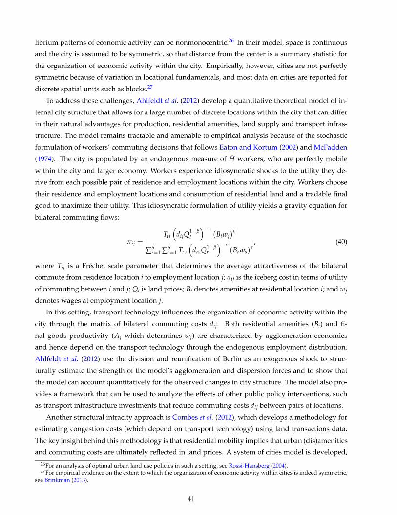
librium patterns of economic activity can be nonmonocentric.26 In their model, space is continuous

and the city is assumed to be symmetric, so that distance from the center is a summary statistic for

the organization of economic activity within the city. Empirically, however, cities are not perfectly

symmetric because of variation in locational fundamentals, and most data on cities are reported for

discrete spatial units such as blocks.27

To address these challenges, Ahlfeldt et al. (2012) develop a quantitative theoretical model of in-

ternal city structure that allows for a large number of discrete locations within the city that can differ

in their natural advantages for production, residential amenities, land supply and transport infras-

tructure. The model remains tractable and amenable to empirical analysis because of the stochastic

formulation of workers’ commuting decisions that follows Eaton and Kortum (2002) and McFadden

(1974). The city is populated by an endogenous measure of H workers, who are perfectly mobile

within the city and larger economy. Workers experience idiosyncratic shocks to the utility they de-

rive from each possible pair of residence and employment locations within the city. Workers choose

their residence and employment locations and consumption of residential land and a tradable final

good to maximize their utility. This idiosyncratic formulation of utility yields a gravity equation for

bilateral commuting flows:

πij =Tij

(dijQ

1−βi

)−ε (Biwj

)ε

∑Sr=1 ∑S

s=1 Trs

(drsQ1−β

r

)−ε(Brws)

ε, (40)

where Tij is a Frechet scale parameter that determines the average attractiveness of the bilateral

commute from residence location i to employment location j; dij is the iceberg cost in terms of utility

of commuting between i and j; Qi is land prices; Bi denotes amenities at residential location i; and wj

denotes wages at employment location j.

In this setting, transport technology influences the organization of economic activity within the

city through the matrix of bilateral commuting costs dij. Both residential amenities (Bi) and fi-

nal goods productivity (Aj which determines wj) are characterized by agglomeration economies

and hence depend on the transport technology through the endogenous employment distribution.

Ahlfeldt et al. (2012) use the division and reunification of Berlin as an exogenous shock to struc-

turally estimate the strength of the model’s agglomeration and dispersion forces and to show that

the model can account quantitatively for the observed changes in city structure. The model also pro-

vides a framework that can be used to analyze the effects of other public policy interventions, such

as transport infrastructure investments that reduce commuting costs dij between pairs of locations.

Another structural intracity approach is Combes et al. (2012), which develops a methodology for

estimating congestion costs (which depend on transport technology) using land transactions data.

The key insight behind this methodology is that residential mobility implies that urban (dis)amenities

and commuting costs are ultimately reflected in land prices. A system of cities model is developed,

26For an analysis of optimal urban land use policies in such a setting, see Rossi-Hansberg (2004).27For empirical evidence on the extent to which the organization of economic activity within cities is indeed symmetric,

see Brinkman (2013).

41

in which each city is monocentric and workers face costs of commuting to the Central Business Dis-

trict (CBD). The model highlights that the elasticity of urban costs with respect to city population

is the product of three quantities: the elasticity of unit land prices at the city centre with respect

to population, the share of land in housing, and the share of housing in consumption expenditure.

Implementing this methodology, the paper’s preferred estimates for these three elasticities are 0.72,

0.25 and 0.23 respectively. Taking the product of these three parameters, the preferred elasticity of

urban costs with respect to city population is 0.041, which is close to existing estimates of agglomer-

ation economies in the form of the elasticity of city productivity with respect to city population. This

finding that cities operate near aggregate constant returns to scale suggests that the fundamental

trade-off of spatial economics – between agglomeration economies and congestion costs – may play

only a limited role in explaining the observed distribution of city sizes. This prediction is in turn

consistent with the observation that cities of vastly different sizes exist and prosper.

7 Conclusion

To determine the causal effect of infrastructure on the spatial organization of economic activity, the

central inference problem that researchers must overcome is that infrastructure is not assigned to

locations at random, but rather on the basis of many of the same unobserved location character-

istics that affect economic activity. The recent empirical literature is organized around three main

approaches to this problem, planned routes IV, historical routes IV and the inconsequential places

approach. While these approaches remain open to criticism and refinement, they are about as good

as can be hoped for in an environment where experiments seem implausible.

This literature suggests a number of tentative conclusions about the effects of infrastructure. Most

studies estimate that population or employment density falls between 6 and 15% with a doubling

of the distance to a highway or railroad (where railroads are the primary mode of transportation).

Highways decentralize urban populations, and with less certainty, manufacturing activity. They

may also lead to a complementary concentration of services. Different sectors appear to respond

differently to different modes of transportation and people respond differently than firms. The effects

of infrastructure seem similar across countries at different stages of development.

While much effort has been directed to unraveling the problem of non-random assignment of

infrastructure to places, much less has been directed to distinguishing between growth and reorga-

nization. This distinction is clearly central to any understanding of the role of infrastructure and

transportation costs in an economy. We suggest two approaches to resolving this problem. The first

is a two equation generalization of the current single equation reduced form models. The second

relies on our structural model to resolve this problem. With this said, the literature does suggest that

much of the estimated effect of transportation costs and infrastructure on the spatial organization of

economic activity is probably due to reorganization rather than growth. Refining our understanding

of this issue seems an obvious place for further research.

42

In addition to the largely reduced-form literature currently available, structural models of trans-

portation costs and the spatial organization of economic activity are beginning to appear. Structural

models have the important advantage of allowing for estimates of general equilibrium effects, such

as the migration of economic activity in response to changes in transportation costs, on the basis

of theoretically founded estimating equations. They also have obvious advantages for welfare and

counterfactual analysis: available results suggest the importance of the ‘share of trade with self’ as an

indicator of welfare. With this said, there is disagreement in the literature on fundamental assump-

tions underlying these models. In particular, whether we should think of cities as drawing people

from the countryside or as competing with cities other for residents. Resolving this issue appears to

be an important prerequisite for further progress.

Finally, the existing literature has devoted little attention, empirical or theoretical, to the dynamics

of how transportation infrastructure affects economic development. In particular, there are few panel

data studies conducting impulse response estimates. This seems to be an important, though difficult

area for further research.

References

Ahlfeldt, Gabriel M., Stephen J. Redding, Daniel M. Sturm, and Nikolaus Wolf. 2012. The economics

of density: Evidence from the Berlin Wall. CEP Discussion Paper No. 1154, London School of

Economics.

Allen, Treb and Costas Arkolakis. 2013. Trade and the topography of the spatial economy. Processed,

Yale University.

Alonso, William. 1964. Location and land use: Toward a general theory of land rent. Cambridge, MA:

Harvard University Press.

Anderson, James E. and Eric van Wincoop. 2003. Gravity with gravitas: A solution to the border

puzzle. American Economic Review 93(1):170–192.

Angel Garcia-Lopez, Miquel. 2012. Urban spatial structure, suburbanization and transportation in

Barcelona. Journal of Urban Economics 72:176–190.

Atalay, Enghin, Ali Hortacsu, and Chad Syverson. 2013. Vertical integration and input flows. Pro-

cessed, University of Chicago.

Banerjee, Abhijit, Esther Duflo, and Nancy Qian. 2012. On the road: Transportation infrastructure

and economic growth in China. Technical report, NBER Working Paper no. 17897.

Baum-Snow, Nathaniel. 2007. Did highways cause suburbanization? Quarterly Journal of Economics

122(2):775–805.

43

Baum-Snow, Nathaniel, Loren Brandt, J. Vernon Henderson, Matthew A. Turner, and Qinghua

Zhang. 2012. Roads, railroads and decentralization of Chinese cities. Processed, University of

Toronto.

Baum-Snow, Nathaniel and Matthew E. Kahn. 2005. Effects of urban rail transit expansions: Evidence

from sixteen cities, 1970-2000. Brookings-Wharton Papers on Urban Affaires: 2005 1(4):147–197.

Bernhofen, Daniel M., Zouheir El-Sahli, and Richard Kneller. 2013. Estimating the effects of con-

tainerization on world trade. Processed, University of Nottingham.

Billings, Stephen B. 2011. Estimating the value of a new transit option. Regional Science and Urban

Economics 41(6):525–536.

Bleakley, Hoyt and Jeffrey Lin. 2012. Portage: Path dependence and increasing returns in U.S. history.

Quarterly Journal of Economics 127:587–644.

Bogart, Dan. 2009. Turnpike trusts and property income: New evidence on the effects of transport

improvements and legislation in eighteenth-century England. Economic History Review 62(1):128–

152.

Brinkman, Jeffrey C. 2013. Transportation technologies, agglomeration, and the structure of cities.

Processed, Philadelphia Federal Reserve Bank.

Bureau of Labour Statistics. 2012. Consumer expenditure survey: Average annual expenditures and

characteristics of all consumer units. www.bls.gov. Accessed: 2013-06-01.

Bureau of Transportation Statistics. 2012a. National transportation statistics: Table 1-49, US ton-miles

of freight. www.rita.dot.gov. Accessed: 2013-05-21.

Bureau of Transportation Statistics. 2012b. National transportation statistics: Table 3-23, employment

in for-hire transportation and selected related industries. www.rita.dot.gov. Accessed: 2013-05-02.

Census Bureau. 2009. Commuting (journey to work): Travel time tables. www.census.gov. Accessed:

2013-06-01.

Chandra, Amitabh and Eric Thompson. 2000. Does public infrastructure affect economic activity?

Evidence from the rural interstate highway system. Regional Science and Urban Economics 30(4):457–

490.

China Data Online. 2010. China statistical yearbook 2010: Table 16-9, freight ton-kilometers.

www.chinadataonline.org. Accessed: 2013-05-23.

China Data Online. 2011. China statistical yearbook 2011: Tables 10-5 (urban) and 10-25 (rural).

www.chinadataonline.org. Accessed: 2013-06-18.

44

Clark, Ximena, David Dollar, and Alejandro Micco. 2004. Port efficiency, maritime transport costs,

and bilateral trade. Journal of Development Economics 75(2):417–450.

Combes, Pierre-Philippe, Gilles Duranton, and Laurent Gobillon. 2012. The costs of agglomeration:

Land prices in French cities. Processed, University of Pennsylvania.

Cosar, Kerem and Pablo Fajgelbaum. 2013. Internal geography, international trade, and regional

specialization. Processed, UCLA.

Couture, Victor, Gilles Duranton, and Matthew A. Turner. 2012. Speed. Processed, University of

Toronto.

Criscuolo, Chiara, Ralf Martin, Henry G. Overman, and John Van Reenen. 2012. The causal effects of

an industrial policy. CEP Discussion Paper No 1113.

Cronon, William. 1991. Nature’s metropolis: Chicago and the Great West. New York: W. W. Norton &

Co.

Davis, Donald R. and David E. Weinstein. 2002. Bones, bombs, and break points: The geography of

economic activity. American Economic Review 92(5):1269–1289.

Davis, Morris A. and Francois Ortalo-Magne. 2011. Household expenditures, wages, rents. Review of

Economic Dynamics 14(2):248–261.

Dekle, Robert, Jonathan Eaton, and Samuel Kortum. 2007. Unbalanced trade. American Economic

Review 97(2):351–55.

Department for Transport. 2012. Table tsgb0306: Greenhouse gas emissions by transport mode.

www.gov.uk. Accessed: 2013-06-08.

Desmet, Klaus and Esteban Rossi-Hansberg. 2013. Urban accounting and welfare. American Economic

Review .

Donaldson, D. and R. Hornbeck. 2013. Railroads and american economic growth: A “market access”

approach. Technical report, NBER working paper no. 19213.

Donaldson, David. 2013. Railroads of the Raj: Estimating the impact of transportation infrastructure.

American Economic Review, forthcoming.

Duranton, Gilles. 2014. Roads and trade in Columbia. Processed, University of Pennsylvania.

Duranton, Gilles, Peter Morrow, and Matthew A. Turner. 2014. Roads and trade: Evidence from the

US. Review of Economic Studies 81(2):681–724.

Duranton, Gilles and Matthew A. Turner. 2011. The fundamental law of road congestion: Evidence

from US cities. American Economic Review 101(6):2616–2652.

45

Duranton, Gilles and Matthew A. Turner. 2012. Urban growth and transportation. Review of Economic

Studies 79(4):1407–1440.

Eaton, Jonathan and Samuel Kortum. 2002. Technology, geography, and trade. Econometrica

70(5):1741–1780.

Eurofound. 2000. Third european survey on working conditions 2000: Figure 37.

www.eurofound.europa.eu. Accessed: 2013-06-17.

Eurostat. 2009. Mean consumption expenditure by detailed coicop level.

www.epp.eurostat.ec.europa.eu. Accessed: 2014-05-18.

Eurostat. 2010. Transport database. www.epp.eurostat.ec.europa.eu. Accessed: 2013-05-01.

Eurostat. 2012. Extra eu27 trade since 1999 by mode of transport(nstr).

www.epp.eurostat.ec.europa.eu. Accessed: 2013-06-17.

Faber, Ben. 2014. Trade integration, market size, and industrialization: Evidence from China’s Na-

tional Trunk Highway system. Review of Economic Studies forthcoming.

Fajgelbaum, Pablo and Stephen Redding. 2013. External integration, structural transformation and

economic development: Evidence from Argentina. Processed, Princeton University.

Fogel, Robert. 1964. Railroads and American economic growth: Essays in econometric history. Baltimore

(MD): Johns Hopkins University Press.

Fujita, Masahisa and Paul Krugman. 1995. When is the economy monocentric? Von Thunen and

Chamberlain unified. Regional Science and Urban Economics 25(4):505–528.

Fujita, Masahisa, Paul Krugman, and Anthony Venables. 1999. The spatial economy: Cities, regions, and

international trade. Cambridge MA: MIT Press.

Fujita, Masahisa and Hideaki Ogawa. 1982. Multiple equilibria and structural transition of non-

monocentric urban configurations. Regional Science and Urban Economics 12(2):161–196.

Garcia-Lopez, Miquel-Angel, Adelheid Holl, and Elisabet Viladecans-Marsal. 2013. Suburbaniza-

tion and highways: When the Romans, the Bourbons and the first cars still shape Spanish cities.

Universitat Autonoma de Barcelona & IEB.

Ghani, Ejaz, Arti Grover Goswami, and William R. Kerr. 2013. Highway to success in India: The

impact of the Golden Quadrilateral project for the location and performance of manufacturing.

World Bank, Policy Research Working Paper 6320.

Gibbons, Stephen and Stephen Machin. 2005. Valuing rail access using transport innovations. Journal

of Urban Economics 57(1):148–169.

46

Glaeser, Edward L., Matthew E. Kahn, and Jordan Rappaport. 2008. Why do the poor live in cities?

The role of public transportation. Journal of Urban Economics 63(1):1–24.

Glaeser, Edward L. and Janet E. Kohlhase. 2004. Cities, regions and the decline of transport costs.

Papers in Regional Science 83(1):197–228.

Glaeser, Edward L. and Giacomo A.M. Ponzetto. 2013. Did the death of distance hurt Detroit and

help New York? NBER Working Paper, 13710.

Gonzalez-Navarro, Marco and Climent Quintana-Domeque. 2013. Roads to development: Experi-

mental evidence from urban road pavement. Processed, University of Toronto.

Gordon, Peter and Rishard Willson. 1984. The determinants of light-rail transit demand - an interna-

tional cross-sectional comparison. Transportation Research Part A: General 18(2):135–140.

Haines, Michael R. and Robert A. Margo. 2008. Railroads and local economic development: The

United States in the 1850s. In Joshua L. Rosenbloom (ed.) Quantitative Economic History: The Good

of Counting. London; New York: Routledge, 78–99.

Head, Keith and Thierry Mayer. 2013. What separates us? sources of resistance to globalization.

Canadian Journal of Economics 46(4):1196–1231.

Helpman, Elhanan. 1998. The size of regions. In Topics in Public Economics: Theoretical and Applied

Analysis. Cambridge: Cambridge University Press, 33–54.

Henderson, J. Vernon, Adam Storeygard, and David N. Weil. 2012. Measuring economic growth

from outer space. American Economic Review 102(2):994–1028.

Hillberry, Russell and David Hummels. 2008. Trade responses to geographic frictions: A decompo-

sition using microdata. European Economic Review 52:527–550.

Hsu, Wen-Tai and Hongliang Zhang. 2012. The fundamental law of highway congestion: Evidence

from national expressways in Japan. Working paper, Department of Economics, The National

University of Singapore.

Hummels, David. 1999. Towards a geography of trade costs. GTAP Working Paper No. 17.

Jedwab, Remi and Alexander Moradi. 2013. Transportation technology and economic change: Evi-

dence from colonial railroads and city growth in Africa. Processed, George Washington University.

Knight, Brian. 2002. Endogenous federal grants and crowd-out of state government spending: The-

ory and evidence from the federal highway aid program. American Economic Review 92(1):71–92.

Krugman, Paul R. 1991. Increasing returns and economic geography. Journal of Political Economy

99(3).

47

Limao, Nuno and Anthony J. Venables. 2001. Infrastructure, geographical disadvantage, transport

costs and trade. World Bank Economic Review 15(3):451–479.

Lucas, Robert E., Jr. and Esteban Rossi-Hansberg. 2002. On the internal structure of cities. Economet-

rica 70(4):1445–1476.

Martincus, Christian Volpe, Jeronimo Carballo, and Ana Cusolito. 2012. Routes, exports, and em-

ployment in developing countries: Following the trace of the Inca roads. Processed, World Bank.

Maystadt, Jean-Francois and Gilles Duranton. 2014. The development push of refugees : Evidence

from Tanzania. Processed, Wharton.

McFadden, Daniel. 1974. The measurement of urban travel demand. Journal of Public Economics

3:303–328.

Michaels, Guy. 2008. The effect of trade on the demand for skill - Evidence from the Interstate High-

way System. Review of Economics and Statistics 90(4):683–701.

Michaels, Guy, Ferdinand Rauch, and Stephen J. Redding. 2012. Urbanization and structural trans-

formation. Quarterly Journal of Economics 127:535–586.

Mills, Edwin S. 1967. An aggregative model of resource allocation in a metropolitan area. American

Economic Review (Papers and Proceedings) 57(2):197–210.

Moses, Leon N. 1958. Location and the theory of production. Quarterly Journal of Economics 72(2):259–

272.

Moses, Leon N. and Harold F. Williamson. 1963. Value of time, choice of mode, and the subsidy issue

in urban transportation. Journal of Political Economy 71(3):247–264.

Muth, Richard F. 1969. Cities and housing. Chicago: University of Chicago Press.

Natural Resources Canada. 2012. Comprehensive energy use database table 8: GHG emissions by

transportation mode. www.oee.nrcan.gc.ca. Accessed: 2013-06-03.

Neumark, David and Helen Simpson. 2014. Place-based policies. In Gilles Duranton, William

Strange, and Vernon Henderson (eds.) Handbook of Regional and Urban Economics, Volume 5. Am-

sterdam: Elsevier North-Holland.

North American Transportation Statistics. 2012a. Table 5-2: Domestic freight activity.

www.nats.sct.gob.mx. Accessed: 2013-05-23.

North American Transportation Statistics. 2012b. Table 7-1: International merchandise trade by

mode. www.nats.sct.gob.mx. Accessed: 2013-06-03.

48

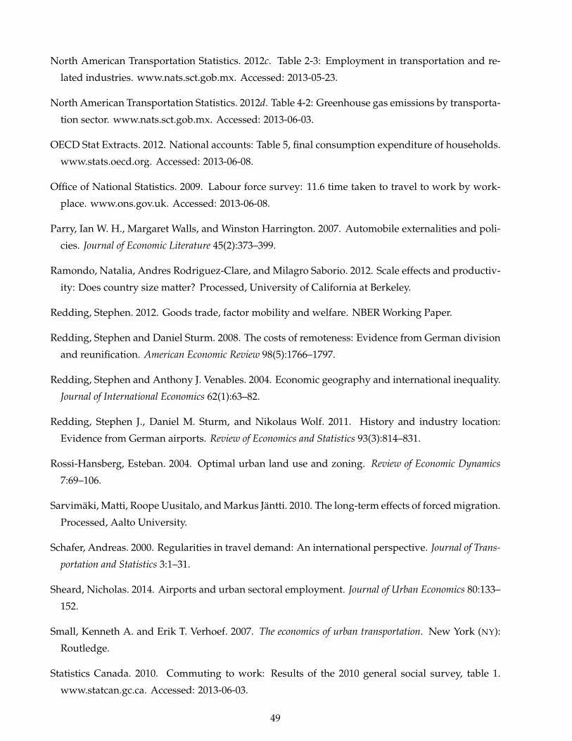
North American Transportation Statistics. 2012c. Table 2-3: Employment in transportation and re-

lated industries. www.nats.sct.gob.mx. Accessed: 2013-05-23.

North American Transportation Statistics. 2012d. Table 4-2: Greenhouse gas emissions by transporta-

tion sector. www.nats.sct.gob.mx. Accessed: 2013-06-03.

OECD Stat Extracts. 2012. National accounts: Table 5, final consumption expenditure of households.

www.stats.oecd.org. Accessed: 2013-06-08.

Office of National Statistics. 2009. Labour force survey: 11.6 time taken to travel to work by work-

place. www.ons.gov.uk. Accessed: 2013-06-08.

Parry, Ian W. H., Margaret Walls, and Winston Harrington. 2007. Automobile externalities and poli-

cies. Journal of Economic Literature 45(2):373–399.

Ramondo, Natalia, Andres Rodriguez-Clare, and Milagro Saborio. 2012. Scale effects and productiv-

ity: Does country size matter? Processed, University of California at Berkeley.

Redding, Stephen. 2012. Goods trade, factor mobility and welfare. NBER Working Paper.

Redding, Stephen and Daniel Sturm. 2008. The costs of remoteness: Evidence from German division

and reunification. American Economic Review 98(5):1766–1797.

Redding, Stephen and Anthony J. Venables. 2004. Economic geography and international inequality.

Journal of International Economics 62(1):63–82.

Redding, Stephen J., Daniel M. Sturm, and Nikolaus Wolf. 2011. History and industry location:

Evidence from German airports. Review of Economics and Statistics 93(3):814–831.

Rossi-Hansberg, Esteban. 2004. Optimal urban land use and zoning. Review of Economic Dynamics

7:69–106.

Sarvimaki, Matti, Roope Uusitalo, and Markus Jantti. 2010. The long-term effects of forced migration.

Processed, Aalto University.

Schafer, Andreas. 2000. Regularities in travel demand: An international perspective. Journal of Trans-

portation and Statistics 3:1–31.

Sheard, Nicholas. 2014. Airports and urban sectoral employment. Journal of Urban Economics 80:133–

152.

Small, Kenneth A. and Erik T. Verhoef. 2007. The economics of urban transportation. New York (NY):

Routledge.

Statistics Canada. 2010. Commuting to work: Results of the 2010 general social survey, table 1.

www.statcan.gc.ca. Accessed: 2013-06-03.

49

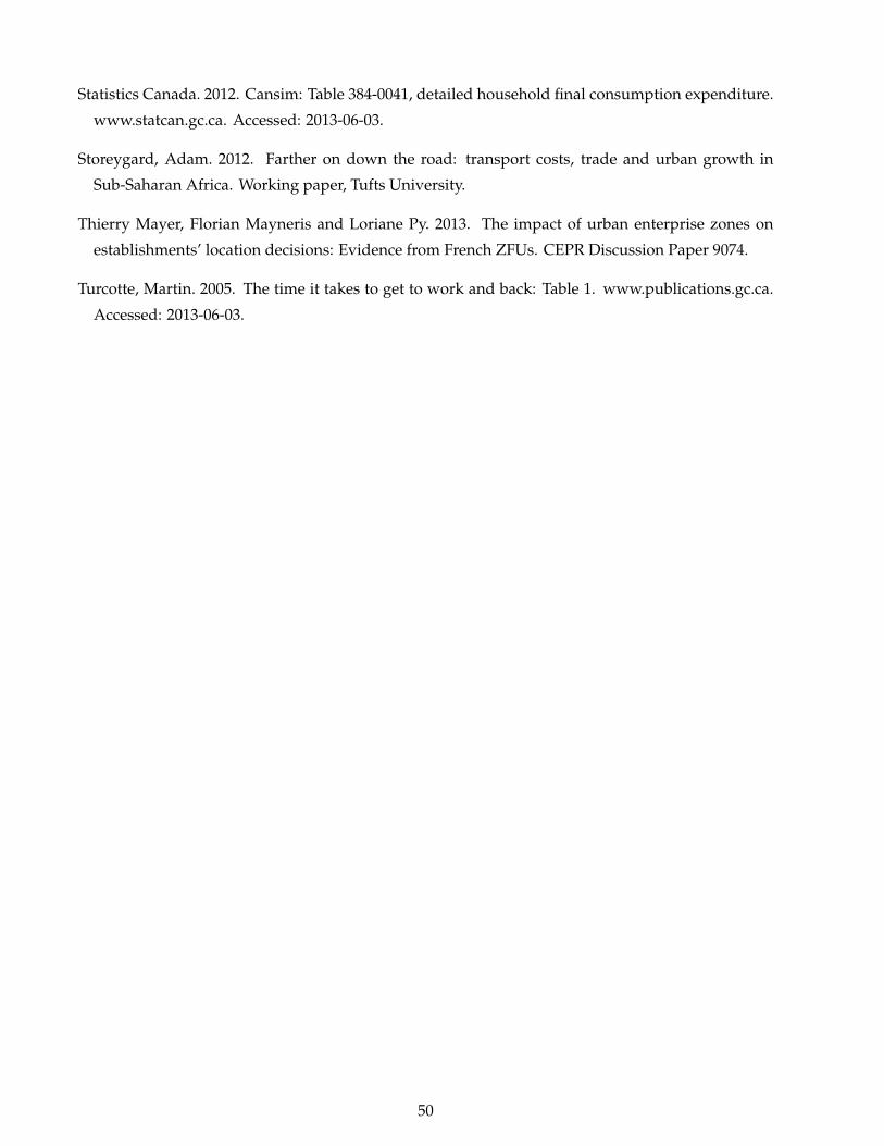
Statistics Canada. 2012. Cansim: Table 384-0041, detailed household final consumption expenditure.

www.statcan.gc.ca. Accessed: 2013-06-03.

Storeygard, Adam. 2012. Farther on down the road: transport costs, trade and urban growth in

Sub-Saharan Africa. Working paper, Tufts University.

Thierry Mayer, Florian Mayneris and Loriane Py. 2013. The impact of urban enterprise zones on

establishments’ location decisions: Evidence from French ZFUs. CEPR Discussion Paper 9074.

Turcotte, Martin. 2005. The time it takes to get to work and back: Table 1. www.publications.gc.ca.

Accessed: 2013-06-03.

50

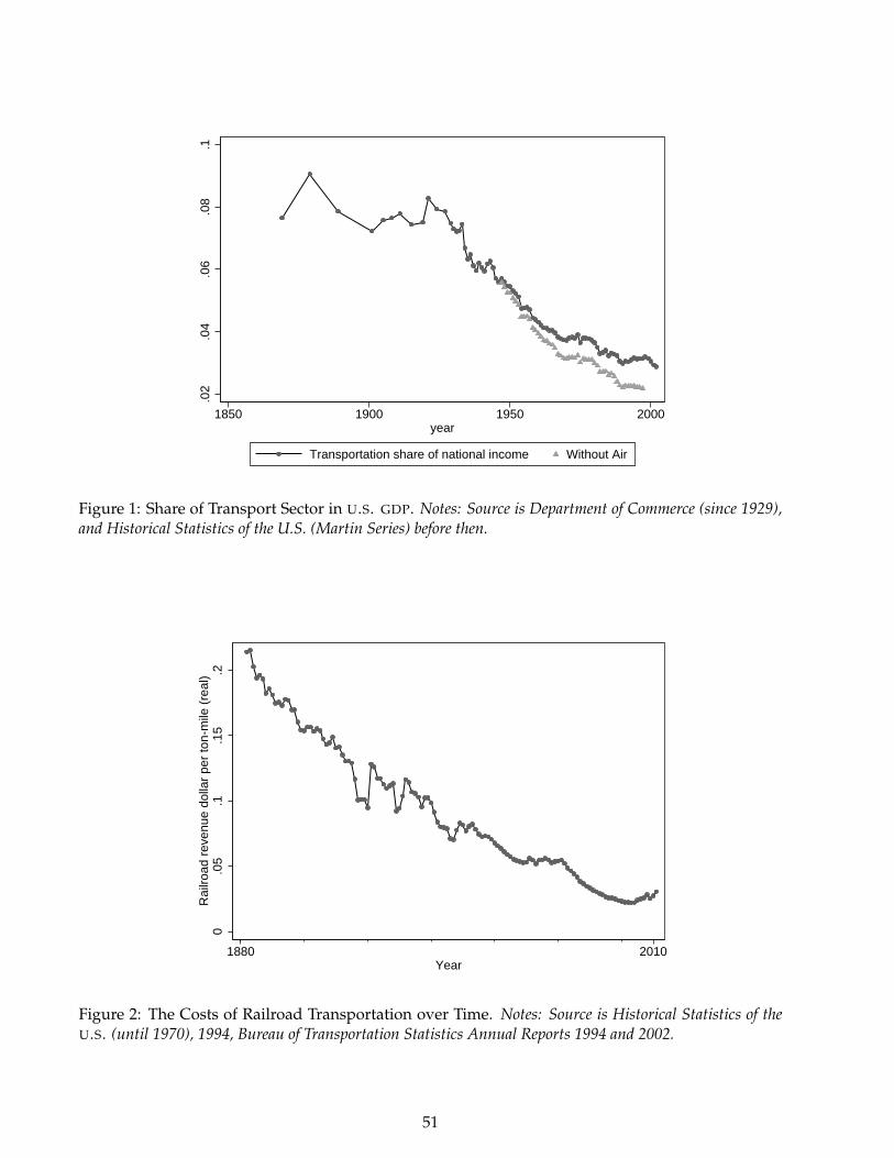
.02

.04

.06

.08

.1

1850 1900 1950 2000year

Transportation share of national income Without Air

Figure 1: Share of Transport Sector in U.S. GDP. Notes: Source is Department of Commerce (since 1929),and Historical Statistics of the U.S. (Martin Series) before then.

0.0

5.1

.15

.2R

ailro

ad r

even

ue d

olla

r pe

r to

n-m

ile (

real

)

1880 2010Year

Figure 2: The Costs of Railroad Transportation over Time. Notes: Source is Historical Statistics of theU.S. (until 1970), 1994, Bureau of Transportation Statistics Annual Reports 1994 and 2002.

51

0.1

.2.3

.4F

reig

ht r

even

ue p

er to

n-m

ile

1960 1970 1980 1990 2000Year

Rail TruckPipe

Figure 3: Revenue per Ton Mile (All Modes). Notes: Source is Bureau of Transportation Statistics AnnualReports.

050

010

0015

0020

00B

illio

ns o

f fre

ight

ton-

mile

1960 1970 1980 1990 2000 2010year

Rail TruckPipe WaterAir

Figure 4: Ton Miles of Freight over Time. Notes: Source is Bureau of Transportation Statistics AnnualReports

52

050

010

00B

illio

ns o

f ton

ne-k

ilom

etre

s

1990 1995 2000 2005 2010Year

Canada domestic frieght activity

050

0010

000

1500

0B

illio

ns o

f ton

ne-k

ilom

etre

s

1980 1990 2000 2010Year

China domestic frieght activity

Source: North American Transportation Statistics (2012a) Source: China Data Online (2010)

020

0040

0060

00B

illio

ns o

f ton

ne-k

ilom

etre

s

1960 1970 1980 1990 2000 2010Year

US domestic frieght activity

010

020

030

0B

illio

ns o

f ton

ne-k

ilom

etre

s

1990 1995 2000 2005 2010Year

Mexico domestic frieght activity

Source: Bureau of Transportation Statistics (2012a) Source: North American Transportation Statistics (2012a)

010

020

0B

illio

ns o

f ton

ne-k

ilom

etre

s

1985 1990 1995 2000 2005 2010Year

Italy domestic frieght activity

010

20B

illio

ns o

f ton

ne-k

ilom

etre

s

2002 2004 2006 2008 2010 2012Year

Lithuania domestic frieght activity

Source: Eurostat (2010) Source: Eurostat (2010)

010

020

030

0B

illio

ns o

f ton

ne-k

ilom

etre

s

1955 1965 1975 1985 1995 2005Year

UK domestic frieght activity

Source: Eurostat (2010)

Figure 5: Ton km of freight by year and mode for several countries.

53

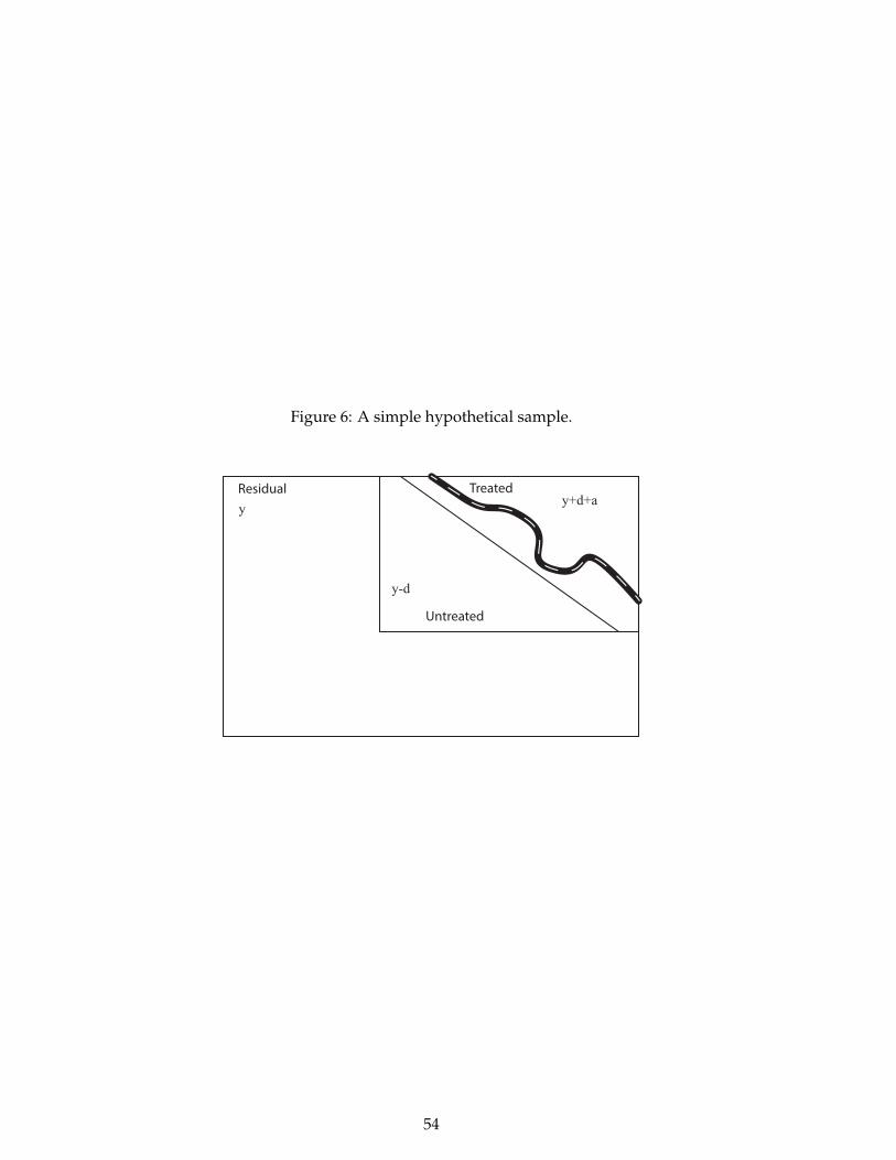
Figure 6: A simple hypothetical sample.

Untreated

Treatedy

y-d

y+d+aResidual

54

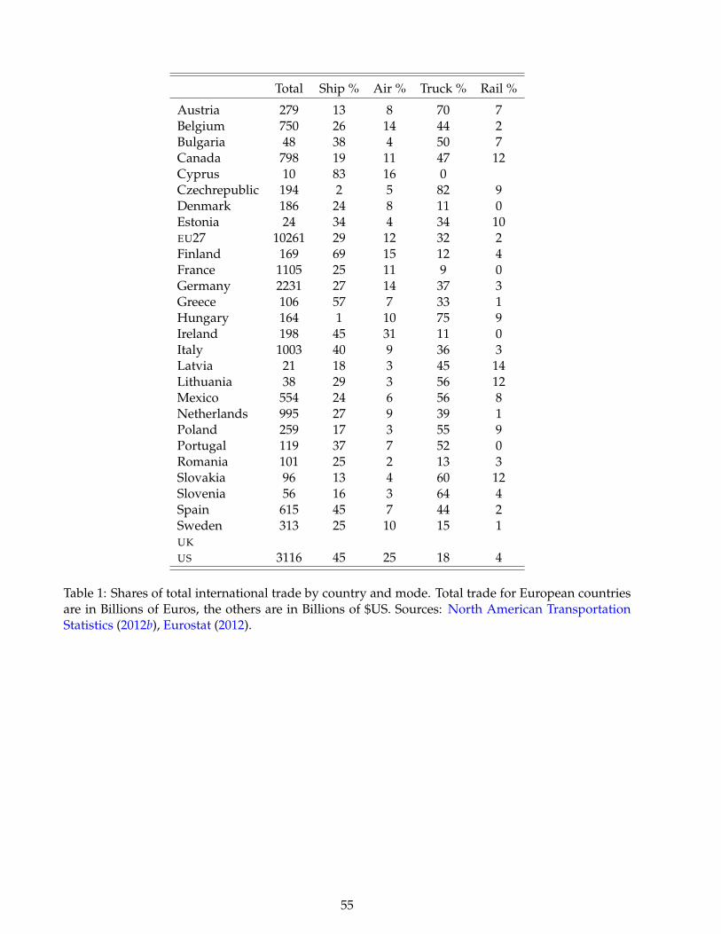
Total Ship % Air % Truck % Rail %

Austria 279 13 8 70 7Belgium 750 26 14 44 2Bulgaria 48 38 4 50 7Canada 798 19 11 47 12Cyprus 10 83 16 0Czechrepublic 194 2 5 82 9Denmark 186 24 8 11 0Estonia 24 34 4 34 10EU27 10261 29 12 32 2Finland 169 69 15 12 4France 1105 25 11 9 0Germany 2231 27 14 37 3Greece 106 57 7 33 1Hungary 164 1 10 75 9Ireland 198 45 31 11 0Italy 1003 40 9 36 3Latvia 21 18 3 45 14Lithuania 38 29 3 56 12Mexico 554 24 6 56 8Netherlands 995 27 9 39 1Poland 259 17 3 55 9Portugal 119 37 7 52 0Romania 101 25 2 13 3Slovakia 96 13 4 60 12Slovenia 56 16 3 64 4Spain 615 45 7 44 2Sweden 313 25 10 15 1UK

US 3116 45 25 18 4

Table 1: Shares of total international trade by country and mode. Total trade for European countriesare in Billions of Euros, the others are in Billions of $US. Sources: North American TransportationStatistics (2012b), Eurostat (2012).

55

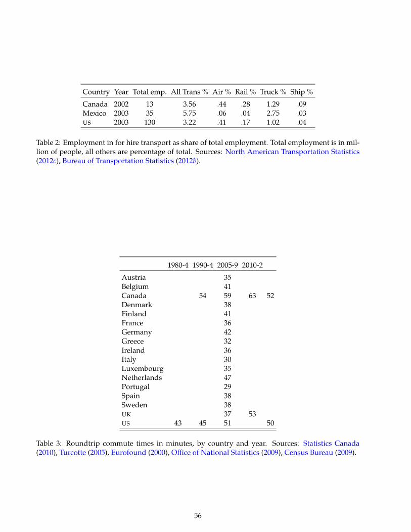
Country Year Total emp. All Trans % Air % Rail % Truck % Ship %

Canada 2002 13 3.56 .44 .28 1.29 .09Mexico 2003 35 5.75 .06 .04 2.75 .03US 2003 130 3.22 .41 .17 1.02 .04

Table 2: Employment in for hire transport as share of total employment. Total employment is in mil-lion of people, all others are percentage of total. Sources: North American Transportation Statistics(2012c), Bureau of Transportation Statistics (2012b).

1980-4 1990-4 2005-9 2010-2

Austria 35Belgium 41Canada 54 59 63 52Denmark 38Finland 41France 36Germany 42Greece 32Ireland 36Italy 30Luxembourg 35Netherlands 47Portugal 29Spain 38Sweden 38UK 37 53US 43 45 51 50

Table 3: Roundtrip commute times in minutes, by country and year. Sources: Statistics Canada(2010), Turcotte (2005), Eurofound (2000), Office of National Statistics (2009), Census Bureau (2009).

56

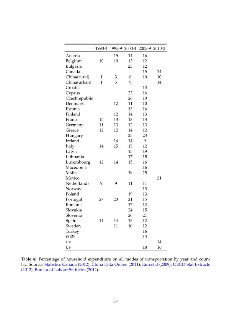
1990-4 1995-9 2000-4 2005-9 2010-2

Austria 15 14 16Belgium 10 10 13 12Bulgaria 23 12Canada 15 14China(rural) 1 3 6 10 10China(urban) 1 5 9 14Croatia 13Cyprus 23 16Czechrepublic 26 19Denmark 12 11 10Estonia 13 16Finland 12 14 13France 15 13 13 13Germany 11 13 12 13Greece 12 12 14 12Hungary 25 23Ireland 14 14 9Italy 14 15 15 12Latvia 15 19Lithuania 17 15Luxembourg 12 14 15 16Macedonia 16Malta 19 25Mexico 21Netherlands 9 9 11 11Norway 13Poland 19 13Portugal 27 23 21 15Romania 17 12Slovakia 24 15Slovenia 26 21Spain 14 14 15 12Sweden 11 10 12Turkey 16EU27 13UK 14US 18 16

Table 4: Percentage of household expenditure on all modes of transportation by year and coun-try. Sources:Statistics Canada (2012), China Data Online (2011), Eurostat (2009), OECD Stat Extracts(2012), Bureau of Labour Statistics (2012).

57

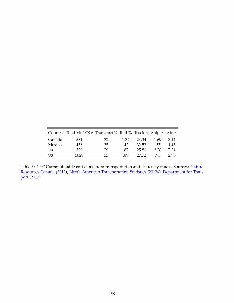
Country Total Mt CO2e Transport % Rail % Truck % Ship % Air %

Canada 561 32 1.32 24.34 1.69 3.14Mexico 456 35 .42 32.53 .57 1.43UK 529 29 .87 25.81 2.38 7.24US 5829 33 .89 27.72 .95 2.96

Table 5: 2007 Carbon dioxide emissions from transportation and shares by mode. Sources: NaturalResources Canada (2012), North American Transportation Statistics (2012d), Department for Trans-port (2012).

58