Transportability across studies: A formal approach

Judea Pearl and Elias Bareinboim∗

Computer Science DepartmentUniversity of California, Los AngelesLos Angeles, CA, 90095-1596, USAjudea@cs.ucla.edu, eb@cs.ucla.edu

April 12, 2013

Abstract

We provide a formal definition of the notion of “transportability,” or “externalvalidity,” which we view as a license to transfer causal information learned in exper-imental studies to a different environment, in which only observational studies canbe conducted. We introduce a formal representation called “selection diagrams” forexpressing knowledge about differences and commonalities between populations of in-terest and, using this representation, we derive procedures for deciding whether causaleffects in the target environment can be inferred from experimental findings in a dif-ferent environment. When the answer is affirmative, the procedures identify the set ofexperimental and observational studies that need be conducted to license the transport.We further demonstrate how transportability analysis can guide the transfer of knowl-edge among non-experimental studies to minimize re-measurement cost and improveprediction power. We further provide a causally principled definition of “surrogateendpoint” and show that the theory of transportability can assist the identification ofvalid surrogates in a complex network of cause-effect relationships.

1 Introduction: Threats vs. Assumptions

Science is about generalization, and generalization requires transportability. Conclusionsthat are obtained in a laboratory setting are transported and applied elsewhere, in an envi-ronment that differs in many aspects from that of the laboratory.

We all understand that if the target environment is arbitrary, or drastically differentfrom the study environment nothing can be learned and scientific progress will come to astandstill. However, the fact that most studies are conducted with the intention of applyingthe results elsewhere means that we usually deem the target environment sufficiently similarto the study environment to justify the transport of some experimental results or modified

∗This research was supported in parts by NIH grant #1R01 LM009961-01, NSF grant #IIS-0914211, andONR grant #N000-14-09-1-0665.

1

TECHNICAL REPORT R-372

April 2013

versions thereof. Cox (1958) indeed noted that extrapolation across studies requires “someunderstanding of the reasons for the differences” (p. 11).

Remarkably, the conditions that permit such transport have not received systematicformal treatment. The standard literature on this topic, falling under rubrics such as “quasi-experiments,” “meta analysis,” “heterogeneity,” and “external validity,”1 consists primarilyof “threats,” namely, verbal narratives of what can go wrong when we try to transport resultsfrom one study to another (e.g., Shadish et al. (2002, chapter 3), Hofler et al. (2010)). Rarelydo we find an analysis of “licensing assumptions,” namely, formal and transparent conditionsunder which the transport of results across differing environments or populations is licensedfrom first principles.2

The reasons for this asymmetry are several. First, threats are safer to cite than as-sumptions. He who cites “threats” appears prudent, cautious and thoughtful, whereas hewho seeks licensing assumptions is immediately accused of endorsing those assumptions,thus legitimizing unwarranted transport, or of pretending to know in advance when thoseassumptions hold true.

Second, assumptions are self destructive in their honesty. The more explicit the assump-tion, the more criticism it invites, for it tends to trigger a richer space of alternative scenariosin which the assumption may fail. Researchers prefer therefore to declare threats in publicand make assumptions in private.

Third, whereas threats can be communicated in plain English, supported by anecdotalpointers to familiar experiences, assumptions require a formal language within which thenotion “environment” (or “population”) is given precise characterization, and differencesamong environments can be encoded and analyzed.

The advent of causal diagrams (Pearl, 1995; Greenland et al., 1999; Spirtes et al., 2000;Pearl, 2009) provides such a language and renders the formalization of transportability pos-sible. Armed with this language, this paper departs from the tradition of communicating“threats” and embarks instead on the more adventurous task of formulating “licenses totransport,” namely, assumptions that, if held true, would permit us to transport resultsacross studies.

2 Motivating Examples

To motivate our discussion and to demonstrate some of the subtle questions that trans-portability entails, we will consider three simple examples, graphically depicted in Fig. 1.

Example 1 We conduct a randomized trial in Los Angeles (LA) and estimate the causaleffect of exposure X on outcome Y for every age group Z = z as depicted in Fig. 1(a).

1Manski (2007) defines “external validity” as follows: “An experiment is said to have “external validity”if the distribution of outcomes realized by a treatment group is the same as the distribution of outcome thatwould be realized in an actual program.” (Campbell and Stanley, 1963, p. 5) take a slightly broader view:“‘External validity’ asks the question of generalizability: To what population, settings, treatment variables,and measurement variables can this effect be generalized?”

2Hernan and VanderWeele (2011) studied such conditions in the context of compound treatments, wherewe seek to predict the effect of one version of a treatment from experiments with a different version. Theiranalysis is a special case of the theory developed in this paper (Petersen, 2011).

2

X Y X Y X Y

(c)(b)(a)

Z

Z

Z

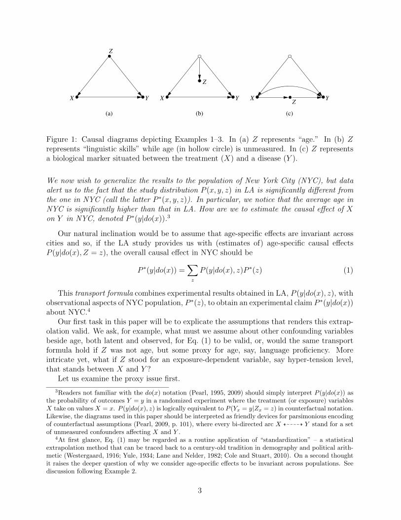
Figure 1: Causal diagrams depicting Examples 1–3. In (a) Z represents “age.” In (b) Zrepresents “linguistic skills” while age (in hollow circle) is unmeasured. In (c) Z representsa biological marker situated between the treatment (X) and a disease (Y ).

We now wish to generalize the results to the population of New York City (NYC), but dataalert us to the fact that the study distribution P (x, y, z) in LA is significantly different fromthe one in NYC (call the latter P ∗(x, y, z)). In particular, we notice that the average age inNYC is significantly higher than that in LA. How are we to estimate the causal effect of Xon Y in NYC, denoted P ∗(y|do(x)).3

Our natural inclination would be to assume that age-specific effects are invariant acrosscities and so, if the LA study provides us with (estimates of) age-specific causal effectsP (y|do(x), Z = z), the overall causal effect in NYC should be

P ∗(y|do(x)) =∑z

P (y|do(x), z)P ∗(z) (1)

This transport formula combines experimental results obtained in LA, P (y|do(x), z), withobservational aspects of NYC population, P ∗(z), to obtain an experimental claim P ∗(y|do(x))about NYC.4

Our first task in this paper will be to explicate the assumptions that renders this extrap-olation valid. We ask, for example, what must we assume about other confounding variablesbeside age, both latent and observed, for Eq. (1) to be valid, or, would the same transportformula hold if Z was not age, but some proxy for age, say, language proficiency. Moreintricate yet, what if Z stood for an exposure-dependent variable, say hyper-tension level,that stands between X and Y ?

Let us examine the proxy issue first.

3Readers not familiar with the do(x) notation (Pearl, 1995, 2009) should simply interpret P (y|do(x)) asthe probability of outcomes Y = y in a randomized experiment where the treatment (or exposure) variablesX take on values X = x. P (y|do(x), z) is logically equivalent to P (Yx = y|Zx = z) in counterfactual notation.Likewise, the diagrams used in this paper should be interpreted as friendly devices for parsimonious encodingof counterfactual assumptions (Pearl, 2009, p. 101), where every bi-directed arc X L9999K Y stand for a setof unmeasured confounders affecting X and Y .

4At first glance, Eq. (1) may be regarded as a routine application of “standardization” – a statisticalextrapolation method that can be traced back to a century-old tradition in demography and political arith-metic (Westergaard, 1916; Yule, 1934; Lane and Nelder, 1982; Cole and Stuart, 2010). On a second thoughtit raises the deeper question of why we consider age-specific effects to be invariant across populations. Seediscussion following Example 2.

3

Example 2 Let the variable Z in Example 1 stand for subjects language proficiency, andlet us assume that Z does not affect exposure (X) or outcome (Y ), yet it correlates withboth, being a proxy for age which is not measured in either study (see Fig. 1(b)). Given theobserved disparity P (z) 6= P ∗(z), how are we to estimate the causal effect P ∗(y|do(x)) forthe target population of NYC from the z-specific causal effect P (y|do(x), z) estimated at thestudy population of LA?

The inequality P (z) 6= P ∗(z) in this example may reflect either age difference or differ-ences in the way that Z correlates with age. If the two cities enjoy identical age distributionsand NYC residents acquire linguistic skills at a younger age, then, since Z has no effect what-soever on X and Y , the inequality P (z) 6= P ∗(z) can be ignored and, intuitively, the propertransport formula would be

P ∗(y|do(x)) = P (y|do(x)) (2)

If, on the other hand, the conditional probabilities P (z|age) and P ∗(z|age) are the same inboth cities, and the inequality P (z) 6= P ∗(z) reflects genuine age differences, Eq. (2) is nolonger valid, since the age difference may be a critical factor in determining how people reactto X. We see, therefore, that the choice of the proper transport formula depends on thecausal context in which population differences are embedded.

This example also demonstrates why the invariance of Z-specific causal effects shouldnot be taken for granted. While justified in Example 1, with Z = age, it fails in Example2, in which Z was equated with “language skills.” Indeed, using Fig. 1(b) for guidance, theZ-specific effect of X on Y in NYC is given by:

P ∗(y|do(x), z) =∑age

P ∗(y|do(x), z, age)P ∗(age|do(x), z)

=∑age

P ∗(y|do(x), age)P ∗(age|z)

=∑age

P (y|do(x), age)P ∗(age|z)

Thus, if the two populations differ in the relation between age and skill, i.e.,

P (age|z) 6= P ∗(age|z)

the skill-specific causal effect would differ as well.The intuition is clear. A NYC person at skill level Z = z is likely to be in a totally

different age group from his skill-equals in Los Angeles and, since it is age, not skill thatshapes the way individuals respond to treatment, it is only reasonable that Los Angelesresidents would respond differently to treatment than their NYC counterparts at the verysame skill level.

The essential difference between Examples 1 and 2 is that age is normally taken to be anexogenous variable (not assigned by other factors in the model) while skills may be indicativeof earlier factors (age, education, ethnicity) capable of modifying the causal effect. Therefore,conditional on skill, the effect may be different in the two populations.

4

Example 3 Examine the case where Z is a X-dependent variable, say a disease bio-marker,standing on the causal pathways between X and Y as shown in Fig. 1(c). Assume furtherthat the disparity P (z) 6= P ∗(z) is discovered in each level of X and that, again, both theaverage and the z-specific causal effect P (y|do(x), z) are estimated in the LA experiment,for all levels of X and Z. Can we, based on information given, estimate the average (orz-specific) causal effect in the target population of NYC?5

Here, Eq. (1) is wrong for two reasons. First, as in the case of age-proxy, it matterswhether the disparity in P (z) represents differences in susceptibility to X or differences inpropensity to receiving X. In the latter case, Eq. (2) would be valid, while in the former,more information is needed. Second, the overall causal effect (in both LA and NYC) is nolonger a simple average of the z-specific causal effects. To witness, consider an unconfoundedMarkov chain X → Z → Y ; the z-specific causal effect P (y|do(x), z) is P (y|z), independentof x, while the overall causal effect is P (y|do(x)) = P (y|x) which is clearly dependent on x.The latter could not be obtained by averaging over the former. The correct weighing rule is

P (y|do(x)) =∑z

P (y, z|do(x)) (3)

=∑z

P (y|do(x), z)P (z|do(x)) (4)

which reduces to (1) only in the special case where Z is unaffected by X, as is the casein Fig. 1(a). Thus, in general, both P (y|do(x), z) and P (z|do(x)) need be measured in theexperiment before we can transport results to populations with differing characteristics. Inthe Markov chain example, if the disparity in P (z) stems only from a difference in people’ssusceptibility to X (say, due to preventive measures taken in one city and not the other)then the correct transport formula would be

P ∗(y|do(x)) =∑z

P (y|do(x), z)P ∗(z|x) (5)

=∑z

P (y|z)P ∗(z|x) (6)

which is different from both (1) and (2), and hardly makes any use of experimental findings.In case X and Y are confounded and directly connected, as in Fig. 1(c), it is Eq. (5)

which provides the correct transport formula (to be proven in Section 4), calling for thez-specific effects to be weighted by the conditional probabilities P ∗(z|x), estimated at thetarget population.

5This is precisely the problem that motivated the unsettled literature on “surrogate endpoint” (Prentice,1989; Freedman et al., 1992; MacKinnon and Dwyer, 1993; Fleming and DeMets, 1996; Burzykowski et al.,2005; Baker, 2006; MacKinnon et al., 2007; Joffe and Green, 2009), that is, finding a way of adjusting fora post-exposure variable Z so as to render effect estimates transportable across populations with differingP (z|do(x)). A solution to this problem will be proposed in Section 6 below.

5

3 Formalizing Transportability

3.1 Selection diagrams and selection variables

A few patterns emerge from the examples discussed in Section 2. First, transportability is acausal, not statistical notion. In other words, the conditions that license transport as well asthe formulas through which results are transported depend on the causal relations betweenthe variables in the domain, not merely on their statistics. When we asked, for example (inExample 3), whether the change in P (z) was due to differences in P (x) or due to a changein the way Z is affected by X, the answer cannot be determined by comparing P (x) andP (z|x) to P ∗(x) and P ∗(z|x). If X and Z are confounded (e.g., Fig. 4(e)), it is quite possiblefor the inequality P (z|x) 6= P ∗(z|x) to hold, reflecting differences in confounding, while theway that Z is affected by X, (i.e., P (z|do(x))) is the same in the two populations.

Second, licensing transportability requires knowledge of the mechanisms, or processes,through which population differences come about; different localization of these mechanismsyield different transport formulae. This can be seen most vividly in Example 2 (Fig. 1(b))where we reasoned that no weighing is necessary if the disparity P (z) 6= P ∗(z) originates withthe way language proficiency depends on age, while the age distribution itself remains thesame. Yet, because age is not measured, this condition cannot be detected in the probabilitydistribution P , and cannot be distinguished from an alternative condition,

P (age) 6= P ∗(age) and P (z|age) = P ∗(z|age)

one that may require weighting according to to Eq. (1). In other words, every probabilitydistribution P (x, y, z) that is compatible with the process of Fig. 1(b) is also compatiblewith that of Fig. 1(a) and, yet, the two processes dictate different transport formulas.

Based on these observations, it is clear that if we are to represent formally the differencesbetween populations (similarly, between experimental settings or environments) we mustresort to a representation in which the causal mechanisms are explicitly encoded and inwhich differences in populations are represented as local modifications of those mechanisms.

To this end, we will use causal diagrams augmented with a set, S, of “selection variables,”where each member of S corresponds to a mechanism by which the two populations differ,and switching between the two populations will be represented by conditioning on differentvalues of these S variables.

Formally, if P (v|do(x)) stands for the distribution of a set V of variables in the exper-imental study (with X randomized) then we designate by P ∗(v|do(x)) the distribution ofV if we were to conduct the study on population Π∗ instead of Π. We now attribute thedifference between the two to the action of a set S of selection variables, and write6

P ∗(v|do(x)) = P (v|do(x), s∗).

Of equal importance is the absence of an S variable pointing to Y in Fig. 2(a), which encodesthe assumption that age-specific effects are invariant across the two populations.

6Alternatively, one can represent the two populations’ distributions by P (v|do(x), s), and P (v|do(x), s∗),respectively. The results, however, will be the same, since only the location of S enters the analysis.

6

The selection variables in S may represent either exogenous conditions or endogenousconsequences of factors by which units are selected for the study. For example, the agedisparity P (z) 6= P ∗(z) discussed in Example 1 will be represented by the inequality

P (z) 6= P (z|s)

where S stands for all factors responsible for drawing subjects at age Z = z to NYC ratherthan LA.

This graphical representation, which we will call “selection diagrams” can also representstructural differences between the two populations. For example, if the causal diagramof the study population contains an arrow between X and Y , and the one for the targetpopulation contains no such arrow, the selection diagram will be X → Y ← S where therole of variable S is to disable the arrow X → Y when S = s∗ (i.e., P (y|x, s∗) = P (y|x′, s∗)for all x′) and reinstate it when S = s.7 Likewise, selection diagrams can easily representdifferences between the intervention used in the experimental study and the one actuallyimplemented on the target population. Our analysis will apply therefore to all factors bywhich populations may differ or that may “threaten” the transport of conclusions betweenstudies, populations, locations or environments.

S

X Y

(c)(b)(a)

Z

S

Z

Z

S

X Y X Y

Figure 2: Selection diagrams depicting Examples 1–3. In (a) the two populations differ inage distributions. In (b) the populations differs in how Z depends on age (an unmeasuredvariable, represented by the hollow circle) and the age distributions are the same. In (c) thepopulations differ in how Z depends on X.

For clarity, we will represent the S variables by squares, as in Fig. 2, which uses selectiondiagrams to encode the three examples discussed in Section 2. In particular, Fig. 2(a) and2(b) represent, respectively, two different mechanisms responsible for the observed disparityP (z) 6= P ∗(z). The first (Fig. 2(a)) dictates transport formula (1) while the second (Fig.2(b)) calls for direct, unadjusted transport (2). Clearly, if the age distribution in the targetpopulation is different relative to that of the study population (Fig. 2(a)) we will representthis difference in the form of an unspecified influence that operates on the age variable Zand results in the difference between P ∗(age) = P (age|S = s∗) and P (age).

7Pearl (1995; 2009, p. 71) and Dawid (2002), for example, use conditioning on auxiliary variables toswitch between experimental and observational studies. Dawid (2002) further uses such variables to representchanges in parameters of probability distributions.

7

In the extreme case, we could add selection nodes to all variables, which means that wehave no reason to believe that the populations share any mechanism in common, and this, ofcourse would inhibit any exchange of conclusions among the populations. Conversely, absenceof a selection node pointing to a variable, say Z, represents an assumption of invariance: thelocal mechanism that assigns values to Z is the same in both populations. Such assumptions,as we will see, will open the door for the transport of some experimental findings.

In this paper, we will address the issue of transportability assuming that scientific knowl-edge about invariance of certain mechanisms is available and encoded in the selection dia-gram through the S nodes. Such knowledge is, admittedly, more demanding than that whichshapes the structure of each causal diagram in isolation. It is, however, a prerequisite forany scientific extrapolation, and constitutes therefore a worthy object of formal analysis.

3.2 Transportability: Definitions and Examples

Using selection diagrams as the basic representational language, and harnessing the conceptsof intervention, do-calculus8 and identifiability (Pearl, 2009, chapter 3) we can now give thenotion of transportability a formal definition.

Definition 1 (Transportability)Given two populations, denoted Π and Π∗, characterized by probability distributions P andP ∗, and causal diagrams G and G∗, respectively, a causal relation R is said to be trans-portable from Π to Π∗ if R(Π) is estimable from the set I of interventional studies on Π,and R(Π∗) is identified from I, P, P ∗, G, and G∗.

Example 4 Let R stand for the causal effect of X on Y , accordingly, R(Π) = P (y|do(x))and R(Π∗) = P ∗(y|do(x)). Let Π and Π∗ be characterized by the causal diagram of Fig.2(a), and let P ∗(x, y, z) differ from P (x, y, z) by the prior probability of Z, i.e., P ∗(x, y, z) =P (x, y, z)P ∗(z)/P (z).

R is transportable from Π to Π∗ when the interventional studies conducted on Π con-tain estimates of the z-specific causal effects, P (y|do(x), z) for all Z = z because, in thiscase, R(Π∗) is identifiable from {P, P ∗, G,G∗, I}, as seen from the Eq. (1). (This will beshown formally in Section 4.) However, R is not transportable from Π to Π∗ when the Icontains only estimates of the overall causal effect P (y|do(x)), because the desired relation,R(Π∗) = P ∗(y|do(x)) cannot be identified from {P, P ∗, G,G∗} and P (y|do(x)). In otherwords, it is possible to construct two models, both compatible with the diagram G, that agreeon P (y|do(x)) but disagree on P (y|do(x), z)). Such construction rules out the identifiabilityof R(Π∗) from {P, P ∗, G,G∗, I}, hence R(Π) is not transportable.

In the sequel we assume that I contains all covariate-specific causal effects that can beestimated from the experimental study on Π, keeping in mind that, transportability is definedmodulo the information set I.

Definition 1 provides a declarative characterization of transportability which, in the-ory, requires one to demonstrate the non-existence of two competing models, agreeing on

8The three rules of do-calculus are given in Appendix 1 and are illustrated in graphical details in (Pearl,2009, p. 87).

8

{P, P ∗, G,G∗, I}, and disagreeing on R(Π∗). Such demonstrations are extremely cumber-some for reasonably sized models, and we seek therefore procedural criteria which, given thepair (G,G∗) will decide the transportability of any given relation directly from the structuresof G and G∗. Such criteria will be developed in Section 4, and will be based on breaking downa complex relation R into more elementary relations which will be recognized immediatelyas transportable. We will formalize the structure of this procedure in Lemma 1, followedby Definitions 2 and 3 below, through which two special cases of transportability will beimmediately recognized.

Lemma 1 Let D be the selection diagram characterizing two populations, Π and Π∗, and Sa set of selection variables in D. The relation R = P (y|do(x), z) is transportable from Π toΠ∗ if and only if the expression P (y|do(x), z, s) is reducible, using the rules of do-calculus,to an expression in which S appears only as a conditioning variable in do-free terms. �

Proof :(if part): Every relation satisfying the condition of Lemma 1 can be written as an algebraiccombination of two kinds of terms, those that involve S and those that do not. The formerscan be written as P ∗ terms and are estimable, therefore, from observations on Π∗, as requiredby Definition 1. All other terms, especially those involving do-operators, do not contain S;they are experimentally identifiable therefore in Π.(only if part): See Corollary 4 in (Bareinboim and Pearl, 2012). �

Definition 2 (Direct Transportability)A causal relation R is said to be directly transportable from Π to Π∗, if R(Π∗) = R(Π).

The equality R(Π∗) = R(Π) means that S can be deleted from the expression of R(Π∗),which satisfies the condition of Lemma 1. A graphical test for direct transportability of thecausal effect P (y|do(x)) follows immediately from do-calculus and reads: (S⊥⊥Y |X)GX

; inwords, X blocks all paths from S to Y once we remove all arrows pointing to X.Remark.The notion of “external validity” as defined by Manski (2007) (footnote 1) corresponds toDirect Transportability, for it requires that R retains its validity without adjustment, asin Eq. (2). Such conditions are rather restrictive for they require in essence that Y beindependent of S for every level of the randomized treatment variable X.

Definition 3 (Trivial Transportability)A causal relation R is said to be trivially transportable from Π to Π∗, if R(Π∗) is identifiablefrom (G∗, P ∗).

This criterion amounts to ordinary (nonparametric) identifiability of causal relationsusing graphs, as defined in Pearl (2009, p. 77), which permits us to estimate R(Π∗) directlyfrom observational studies on Π∗, un-aided by causal information from Π.

Example 5 Let R be the causal effect of X on Y , and let G and G∗ be Markovian diagramsdiffering only in the treatment selection probabilities P (x|pa(X)) and P ∗(x|pa(X)) wherepa(X) are the parents of X in G. Then R is directly transportable, because causal effects areindependent of the selection mechanism (see Pearl, 2009, pp. 72–73).

9

Example 6 Let R be the z-specific causal effect of X on Y P (y|do(x), z) where Z is a setof exogenous pre-treatment covariates. If G = G∗ and P ∗ differs from P only in the priorprobabilities P (z) and P ∗(z), then R is directly transportable. Fig. 2(a) depicts this example.

Example 7 Let R be the z-specific causal effect of X on Y P (y|do(x), z) where Z is aset of variables, and P and P ∗ differ only in the conditional probabilities P (z|pa(Z)) andP ∗(z|pa(Z)) such that Z⊥⊥Y |pa(Z), as shown in Fig. 2(b). Under these conditions, R isnot directly transportable. However, the pa(Z)-specific causal effects P (y|do(x), pa(Z)) aredirectly transportable, and so is P (y|do(x)). Note that, due to the confounding arcs, none ofthese quantities is identifiable.

Example 8 Let R be the causal effect P (y|do(x)) and let the selection diagram of Π and Π∗

be given by X → Y ← S, then R is trivially transportable, since R(Π∗) = P ∗(y|x).

Example 9 Let R be the causal effect P (y|do(x)) and let the selection diagram of Π and Π∗

be given by X → Y ← S, with X and Y confounded as shown in Fig. 4(b), then R is nottransportable, because P ∗(y|do(x)) = P (y|do(x), s) cannot be reduced to a s-free expressionusing the rules of do-calculus. This is the smallest graph for which the causal effect is non-transportable.

4 Transportability of causal effects - A graphical crite-

rion

We now state and prove two theorems that permit us to decide algorithmically, given aselection diagram, whether a relation is transportable between two populations, and whatthe transport formula should be.

Theorem 1 Let D be the selection diagram characterizing two populations, Π and Π∗, andS the set of selection variables in D. The strata-specific causal effect P (y|do(x), z) is trans-portable from Π to Π∗ if Z d-separates Y from S in the X-manipulated version of D, thatis, Z satisfies (Y⊥⊥S|Z)DX

. �

Proof:

P ∗(y|do(x), z) = P (y|do(x), z, s)

From Rule-1 of do-calculus (Pearl, 2009, p. 85) we have: P (y|do(x), z, s) = P (y|do(x), z)whenever Z satisfies (Y⊥⊥S|Z) in DX . This proves Theorem 1.

Definition 4 (S-admissibility)A set T of variables satisfying (Y⊥⊥S|T ) in DX will be called S-admissible (with respect tothe causal effect of X on Y ).

10

S

X Y

S

Z Z

(a)

Y

W

X

(b)

Figure 3: Selection diagrams illustrating S-admissibility. (a) has no S-admissible set whilein (b), W is S-admissible.

Corollary 1 The average causal effect P (y|do(x)) is transportable from Π to Π∗ if thereexists a set Z of observed pre-treatment covariates that is S-admissible. Moreover, the trans-port formula is given by the weighting of Eq. (1). �

Proof:

P ∗(y|do(x)) = P (y|do(x), s) (7)

=∑z

P (y|do(x), z, s)P (z|do(x), s) (8)

=∑z

P (y|do(x), z)P (z|s) (9)

(using S-admissibility and Rule-3 of do-calculus)

=∑z

P (y|do(x), z)P ∗(z) (10)

Example 10 The causal effect is transportable in Fig. 2(a), since Z is S-admissible, andin Fig. 2(b), where the empty set is S-admissible. It is also transportable in Fig. 3(b), whereW is S-admissible, but not in Fig. 3(a) where no S-admissible set exists.

Corollary 2 Any S variable that is pointing directly into X as in Fig. 4(a), or that isd-connected to Y only through X can be ignored.

This follows from the fact that the empty set is S-admissible relative to any such Svariable. Conceptually, the corollary reflects the understanding that differences in propensityto receive treatment do not hinder the transportability of treatment effects; the randomizationused in the experimental study washes away such differences. �

We now generalize Theorem 1 to cases involving treatment-dependent Z variables, as inFig. 2(c).

Theorem 2 The average causal effect P (y|do(x)) is transportable from Π to Π∗ if eitherone of the following conditions holds

11

1. P (y|do(x)) is trivially transportable

2. There exists a set of covariates, Z (possibly affected by X) such that Z is S-admissibleand for which P (z|do(x)) is transportable

3. There exists a set of covariates, W that satisfy (X⊥⊥Y |W,S)D and for which P (w|do(x))is transportable. �

Proof:

1. Condition (1) entails transportability.

2. If condition (2) holds, it implies

P ∗(y|do(x)) = P (y|do(x), s) (11)

=∑z

P (y|do(x), z, s)P (z|do(x), s) (12)

=∑z

P (y|do(x), z)P ∗(z|do(x)) (13)

We now note that the transportability of P (z|do(x)) should reduce P ∗(z|do(x)) to astar-free expression and would render P (y|do(x)) transportable.

3. If condition (3) holds, it implies

P ∗(y|do(x)) =P (y|do(x), s) (14)

=∑w

P (y|do(x), w, s)P (w|do(x), s) (15)

=∑w

P (y|w, s)P ∗(w|do(x)) (16)

(by Rule-3 of do-calculus)

=∑w

P ∗(y|w)P ∗(w|do(x)) (17)

We similarly note that the transportability of P (w|do(x)) should reduce P ∗(w|do(x)) toa star-free expression and would render P (y|do(x)) transportable. This proves Theorem2.

Remark.The test entailed by Theorem 2 is recursive, since the transportability of one causal effectdepends on that of another. However, given that the diagram is finite and feedback-free, thesets Z and W needed in conditions 2 and 3 of Theorem 2 would become closer and closerto X, and the iterative process will terminate after a finite number of steps. This occursbecause the causal effects P (z|do(x)) (likewise, P (w|do(x))) is trivially transportable andequals P (z) for any Z node that is not a descendant of X. Thus, the need for reiterationapplies only to those members of Z that lie on the causal pathways from X to Y .

12

ZY

ZYX

(c)

S

S

XZ

YW

(d)

S

XZ

Y

(e)

S

S S

(a)

(f)

YZ

X

(b)

YY XX

Figure 4: Selection diagrams illustrating transportability. The causal effect P (y|do(x)) is(trivially) transportable in (c) but not in (b) and (f). It is transportable in (a), (d), and (e)(see Corollary 2 and Appendix 2).

Example 11 Applying Theorem 2 to Fig. 2(c), we conclude that R = P (y|do(x)) is triviallytransportable, for it is identifiable in Π∗, through the front-door criterion (Pearl, 2009).It is likewise (trivially) transportable in Fig. 4(c) (by the back-door criterion). R is nottransportable however in Fig. 3(a), where no S-admissible set exists.

Example 12 Fig. 4(d) requires that we invoke both conditions of Theorem 2, iteratively. Tosatisfy condition 2 we note that Z is S-admissible, and we need to prove the transportabilityof P (z|do(x)). To do that, we invoke condition 3 and note that W d-separates X from Zin D. There remains to confirm the transportability of P (w|do(x)), but this is guaranteedby the fact that the empty set is S-admissible relative to W , since W⊥⊥S. Hence, by Theo-rem 1 (replacing Y with W ) P (w|do(x)) is transportable, which bestows transportability onP (y|do(x)). Thus, the final transport formula (derived formally in Appendix 2) is:

P ∗(y|do(x)) =∑z

P (y|do(x), z)∑w

P (w|do(x))P ∗(z|w) (18)

The first two factors on the right are estimable in the experimental study, and the thirdthrough observational studies on the target population. Note that the joint effect P (y, w, z|do(x))need not be estimated in the experiment; a decomposition that results in improved estimationpower.

A similar analysis applies to Fig. 4(e) (see Appendix 2). The model of Fig. 4(f) howeverdoes not allow for the transportability of P (y|do(x)) because there is no S-admissible set inthe diagram and, furthermore, condition 3 of Theorem 2 cannot be invoked.

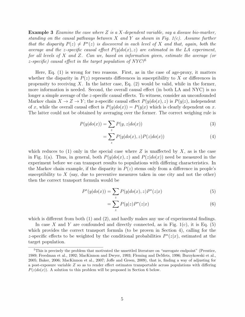
Example 13 To illustrate the power of Theorem 2 in discerning transportability and deriv-ing transport formulae, Fig. 5 represents a more intricate selection diagram, which requiresseveral iteration to discern transportability. The transport formula for this diagram is givenby

13

S

S

ZWX Y

V

T

U

Figure 5: Selection diagram in which the causal effect is shown to be transportable in twoiterations of Theorem 2 (see Appendix 3).

P ∗(y|do(x)) =∑z

P (y|do(x), z)∑w

P ∗(z|w)∑t

P (w|do(x), t)P ∗(t) (19)

The main power of this formula is to guide investigators in deciding what measurementsneed be taken in both the experimental study and the target population. It asserts, forexample, that variables U and V need not be measured. It likewise asserts that theW -specificcausal effects need not be estimated in the experimental study and only the conditionalprobabilities P ∗(z|w) and P ∗(t) need be estimated in the target population. The derivationof this formulae is given in Appendix 3.

Despite its power, Theorem 2 in not complete, namely, it is not guaranteed to approveall transportable relations or to disapprove all non-transportable ones. An example of theformer is given in Appendix 4, the nature of which indicates that the frequency of such caseswill be low in practice.

5 Transportability across Observational Studies

Our analysis thus far assumed that transport is needed from experimental to observationalstudies because R, the relation of interest, is causal and cannot therefore be identified solelyfrom observations in the target population. In this section we demonstrate that transportingfinding among observational studies can be beneficial as well, albeit for different reasons.

Assume we conduct an elaborate observational study in LA, involving dozens of variablesand thousands of samples, aiming to estimate some statistical parameter, R(P ), (that is, afunctional of the population distribution P ). We now wish to estimate the same parameterR(P ∗) in the population of NYC. The question arises whether it is necessary to repeat thestudy from scratch or, in case the disparity between the two populations is localized, we canuse much of what we learned in LA, supplement it with a less elaborate study in NYC andcombine the results to yield an informed estimate of R(P ∗).

In complex models, the savings gained by focusing on only a small subset of variables inP ∗ can be enormous, because any reduction in the number of measured variables translates

14

into substantial reduction in the number of samples needed to achieve a given level of predic-tion accuracy. This is especially true in non-parametric models, where estimation efficiencydeteriorates significantly with the number of variables involved.

An examination of the transport formulas derived in this paper (e.g., Eqs. (10), (18)or (19)) reveals that the methods developed for transporting causal relations are applicableto observational studies as well, albeit with some modification. Consider Eq. (18) and itsassociated diagram in Fig. 4(d). If the target relation R = P ∗(y|do(x)) was expressed, notin terms of the do(x) operator, but as a regression expression R(P ∗) =

∑c P∗(y|x, c)P ∗(c)

where C is a sufficient set of confounders, the right hand side of (18) reveals that P ∗(z|w) isthe only relation that need to be re-estimated at the target population; all the other termsin that expression are estimable from observational studies at the source population, usingC, X, Z, W and Y .

If C is multi-dimensional, or if it requires costly measurements, the savings gained bylimiting the scope of the new study to that of estimating P ∗(z|w) can be very substan-tial. The amount of savings depends of course on how local the disparity between the twopopulations is, whether we can pinpoint the location of this disparity and, not the least,whether we can translate this knowledge into a mathematical expression that unveils thefeasible savings. In our example, the selection diagram of Fig. 4(d) makes that knowledgeexplicit, and the theory of transportability accomplishes the latter task using the calculusof graphical models. Of particular interest is the observation that measurement of Y is notneeded for estimating R(P ∗). Indeed, if Y is an outcome such as patient’s survival timeor student’s future earnings, measurement of Y may be extremely time consuming if notinfeasible in the target population; this is precisely the problem that motivates “surrogateendpoint” analysis, to be discussed in the next section.

These considerations motivate a slightly different definition of transportability, tailoredto observational studies, which emphasizes narrowing the scope of observations rather thanidentification per se.

Definition 5 (Observational Transportability)Given two populations, Π and Π∗, characterized by probability distributions P and P ∗, andcausal diagrams G and G∗, respectively, a statistical relation R(P ) is said to be observation-ally transportable from Π to Π∗ over V ∗ if R(P ∗) is identified from P , P ∗(V ∗), G, and G∗.where P ∗(V ∗) is the marginal distribution of P ∗ over a subset of variables V ∗.

This definition requires that the relation transferred be reconstructed from data obtainedin the old study, plus observations conducted on a subset V ∗ of variables in the new study. Inthe example above, R(P ) was shown to be observationally transportable over V ∗ = {Z,W},while in the example of Fig. 5, we have V ∗ = {Z,W, T} (from Eq. (19)).

It should be noted that the notion of transportability, be it across observational or exper-imental studies requires causal knowledge for its definition. It is the causal diagram G andits associated selection diagram that identify the mechanism by which the two populationsdiffer, hence the mechanisms that remain invariant as one moves from one population toanother. The probabilities P and P ∗, being descriptive, cannot convey information aboutthe locality of the mechanism that accounts for their differences. In Fig. 5, for example,changes in s’ will propagate to the entire probability P (t, u, x, w, y) and could not be distin-guished from changes in an S-node that points, say, at W or at Y . Moreover P and P ∗ can

15

X Y

Z2

(b)

Z2Z1

S

S

(a)

X Y

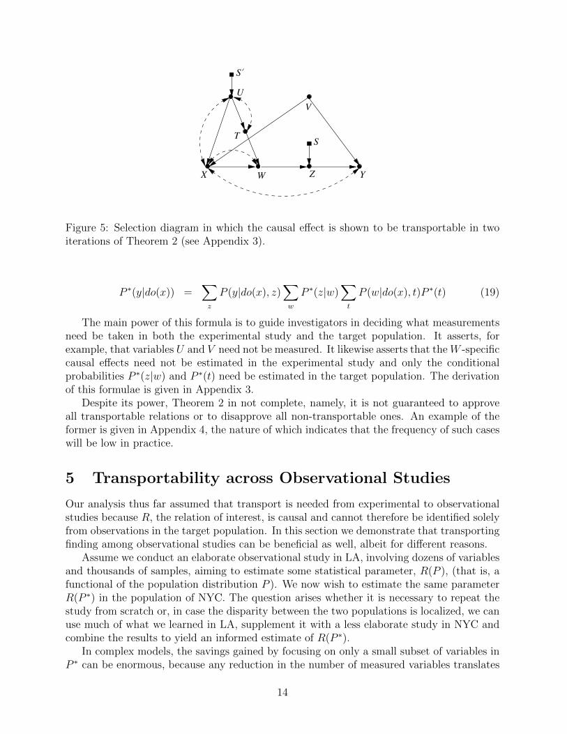
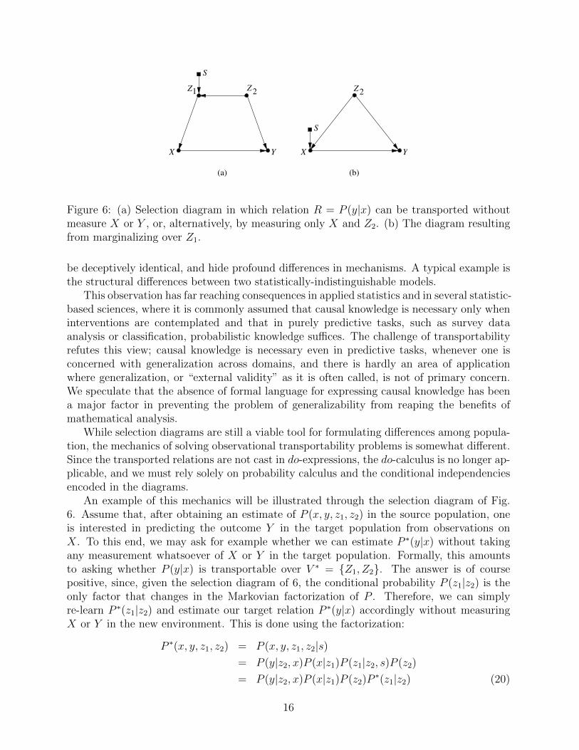
Figure 6: (a) Selection diagram in which relation R = P (y|x) can be transported withoutmeasure X or Y , or, alternatively, by measuring only X and Z2. (b) The diagram resultingfrom marginalizing over Z1.

be deceptively identical, and hide profound differences in mechanisms. A typical example isthe structural differences between two statistically-indistinguishable models.

This observation has far reaching consequences in applied statistics and in several statistic-based sciences, where it is commonly assumed that causal knowledge is necessary only wheninterventions are contemplated and that in purely predictive tasks, such as survey dataanalysis or classification, probabilistic knowledge suffices. The challenge of transportabilityrefutes this view; causal knowledge is necessary even in predictive tasks, whenever one isconcerned with generalization across domains, and there is hardly an area of applicationwhere generalization, or “external validity” as it is often called, is not of primary concern.We speculate that the absence of formal language for expressing causal knowledge has beena major factor in preventing the problem of generalizability from reaping the benefits ofmathematical analysis.

While selection diagrams are still a viable tool for formulating differences among popula-tion, the mechanics of solving observational transportability problems is somewhat different.Since the transported relations are not cast in do-expressions, the do-calculus is no longer ap-plicable, and we must rely solely on probability calculus and the conditional independenciesencoded in the diagrams.

An example of this mechanics will be illustrated through the selection diagram of Fig.6. Assume that, after obtaining an estimate of P (x, y, z1, z2) in the source population, oneis interested in predicting the outcome Y in the target population from observations onX. To this end, we may ask for example whether we can estimate P ∗(y|x) without takingany measurement whatsoever of X or Y in the target population. Formally, this amountsto asking whether P (y|x) is transportable over V ∗ = {Z1, Z2}. The answer is of coursepositive, since, given the selection diagram of 6, the conditional probability P (z1|z2) is theonly factor that changes in the Markovian factorization of P . Therefore, we can simplyre-learn P ∗(z1|z2) and estimate our target relation P ∗(y|x) accordingly without measuringX or Y in the new environment. This is done using the factorization:

P ∗(x, y, z1, z2) = P (x, y, z1, z2|s)= P (y|z2, x)P (x|z1)P (z1|z2, s)P (z2)

= P (y|z2, x)P (x|z1)P (z2)P∗(z1|z2) (20)

16

with all but the last factor transportable from the source environment. Once we have P ∗,the target relation P ∗(y|x) is easily computed by marginalizing P ∗ over Z1 and Z2.

A somewhat less obvious result obtains when we ask to transport the relation

R′ =∑z1

P (y|x, z1)P (z1) (21)

Here we observe that, since Z1 and Z2 are each a sufficient set (i.e., back-door admissible),Z1 is interchangeable with Z2 (Pearl and Paz, 2010) and R′ can be written as:

R′ =∑z2

P (y|x, z2)P (z2) (22)

Therefore, using the independencies (S⊥⊥Y |X,Z2) and (S⊥⊥Z2) shown in the diagram, thetransported relation becomes:

R′(P ∗) =∑z2

P ∗(y|x, z2)P ∗(z2)

=∑z2

P (y|x, z2, s)P (z2|s)

=∑z2

P (y|x, z2)P (z2) (23)

Thus, R′ is transportable over the null set, or “directly transportable” (Definition 2). Thismeans that R′ can be estimated entirely in the source study and applied to the targetpopulation with no additional measurement at all.

We see that, although the selection diagram designates P (z1|z2) as different in the twopopulation, some transported relations permit us to ignore this difference. The conditionalindependencies embedded in the diagram have the capacity to further narrow the scope V ∗ ofvariables that need be measured, so as to minimize measurement cost and sample variability.For example, if the measurement of Z1 is more costly than that of X, R = P (y|x) can betransported over V ∗ = {Z2, X}, instead of {Z2, Z1}, as dictated by Eq. (20). This can beseen by ignoring (or marginalizing over) Z1, which yields the diagram of Fig. 6(b).

When the variables directly impacted by S (e.g., U in Fig. 5) are affected by unmeasuredconfounders, it is not as easy to isolate the conditional probability factors that changes withS, as we did in Fig. 6(a). An examination of Eq. (19) reveals nevertheless that, even in suchcircumstances, certain relations would require a rather narrow scope for transport, i,e., P ∗(t)and P ∗(z|w) in this example. While a systematic analysis of observational transportability isbeyond the scope of this paper, Definition 5 offers a formal characterization of this commonclass of problems, and identifies the basic elements needed for their solution. In particular, itdemonstrates the essential role of causal knowledge, and the effectiveness of inferential toolssuch as selection diagrams and their associated graph-based algorithms.

17

6 On the definition and recognition of surrogate end-

points

6.1 Target for control or predictor of effects

As remarked in footnote 5, the literature on “surrogate endpoint” is concerned with a specialproblem of transportability, in which causal effects on outcome variables are inferred fromthose measured on surrogate variables, often under different conditions. Although traditionaldefinitions for a surrogate endpoint (e.g., Prentice (1989); Freedman et al. (1992); Lin et al.(1997); Buyse and Molenberghs (1998); Buyse et al. (2000)) are based on regressions, theyare unwittingly motivated by causal considerations, and several attempts have been madesince to reformulate surrogacy in causal vocabulary (Frangakis and Rubin, 2002; Gilbert andHudgens, 2008; Joffe and Green, 2009; Wolfson and Gilbert, 2010).

At its core, the problem concerns a randomized trial where one seeks “endpoint surro-gate,” namely, a variable that would allow good predictability of outcome for both treatmentand control. In the words of Ellenberg and Hamilton (1989) “investigators use surrogate end-points when the endpoint of interest is too difficult and/or expensive to measure routinelyand when they can define some other, more readily measurable, endpoint, which is suffi-ciently well correlated with the first to justify its use as a substitute.” Prentice (1989) hasargued that, for the purpose of substitution, strong correlation is not sufficient, and requiredthe true endpoint rate at any follow-up time to be statistically independent of treatment,given the preceding history of the surrogate variable.

Prentice paper was written in 1989, before the legitimization of causal vocabulary. Todaywe understand that he envisioned the surrogate to be a perfect mediator between the treat-ment and the outcome, allowing no direct effect between the two. In Prentice’s own words(Burzykowski et al., 2005, p. 345), “[the condition requires] that there are no pathways thatbypass the surrogate, and that, otherwise, the treatment effect is fully “explained” by thepreceding surrogate history.”

The question arises: Why would perfect mediation (no bypass) be required when the orig-inal motivation was merely predictive, requiring “strong correlation” but no causal relationbetween Z and Y or X and Z? Moreover, why should strong correlation not be sufficient forsurrogacy and, assuming that correlation alone encounters difficulties, how does mediationalleviate these difficulties?

To answer these questions it is instructive to examine carefully the way surroacy is pre-sented by modern writers. “There has been little agreement on an appropriate mathematicalframework or definition for surrogacy and the degree of surrogacy of a variable. In our view,a surrogate outcome is an outcome for which knowing the effect of treatment on the sur-rogate allows prediction of the effect of treatment on the more clinically relevant outcome”(Joffe and Green, 2009).

Shared by most workers in the field, this description lacks a key ingredient: the relation-ship between the two treatments considered, one prevailing when data is available on boththe surrogate (Z) and the endpoint (Y ), and the second, when data on the surrogate aloneare available. Clearly, if the two treatments are identical, the problem is trivially solved,for then, strong correlation between Z and Y in the first study should suffice; all accurate

18

S

X

Z

UY

(b)

S

XZ

Y

(a)

ZY

ZYX

S

XZ

Y

(d) (e)

S

(c)

YX

(f)

WU

Z

YX

Z

S

U

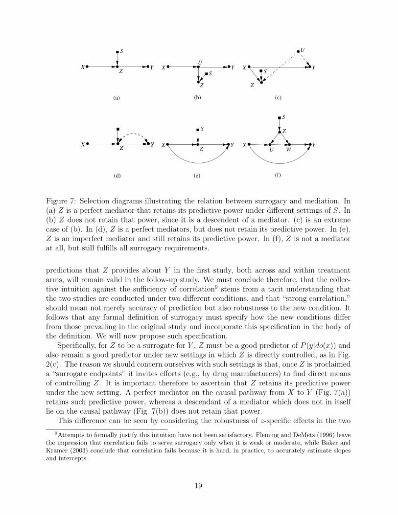
Figure 7: Selection diagrams illustrating the relation between surrogacy and mediation. In(a) Z is a perfect mediator that retains its predictive power under different settings of S. In(b) Z does not retain that power, since it is a descendent of a mediator. (c) is an extremecase of (b). In (d), Z is a perfect mediators, but does not retain its predictive power. In (e),Z is an imperfect mediator and still retains its predictive power. In (f), Z is not a mediatorat all, but still fulfills all surrogacy requirements.

predictions that Z provides about Y in the first study, both across and within treatmentarms, will remain valid in the follow-up study. We must conclude therefore, that the collec-tive intuition against the sufficiency of correlation9 stems from a tacit understanding thatthe two studies are conducted under two different conditions, and that “strong correlation,”should mean not merely accuracy of prediction but also robustness to the new condition. Itfollows that any formal definition of surrogacy must specify how the new conditions differfrom those prevailing in the original study and incorporate this specification in the body ofthe definition. We will now propose such specification.

Specifically, for Z to be a surrogate for Y , Z must be a good predictor of P (y|do(x)) andalso remain a good predictor under new settings in which Z is directly controlled, as in Fig.2(c). The reason we should concern ourselves with such settings is that, once Z is proclaimeda “surrogate endpoints” it invites efforts (e.g., by drug manufacturers) to find direct meansof controlling Z. It is important therefore to ascertain that Z retains its predictive powerunder the new setting. A perfect mediator on the causal pathway from X to Y (Fig. 7(a))retains such predictive power, whereas a descendant of a mediator which does not in itselflie on the causal pathway (Fig. 7(b)) does not retain that power.

This difference can be seen by considering the robustness of z-specific effects in the two

9Attempts to formally justify this intuition have not been satisfactory. Fleming and DeMets (1996) leavethe impression that correlation fails to serve surrogacy only when it is weak or moderate, while Baker andKramer (2003) conclude that correlation fails because it is hard, in practice, to accurately estimate slopesand intercepts.

19

models. In Fig. 7(a), if the Z-specific effect in the initial study is

P (y|do(x), z) = P (y|z)

and will remain the same in the follow up study, since

P (y|do(x), z, s) = P (y|z)

This means that whatever predictions (about the true endpoint Y ) we can make from ob-serving Z in the initial study, those same predictions will remain valid in the followup study,irrespective of the new condition created by S. This is no longer the case in Fig. 7(b). Herethe true endpoint Y can be highly correlated with the putative surrogate Z, for both treat-ment and control, but in the follow up study this correlation may be severely altered, evendestroyed.

A sharper difference emerges between the two models when we consider the role of Z inevaluating the efficacy of new treatments, say S. In Fig. 7(a), the effect of S on Y (whilekeeping X fixed at x) can be evaluated without measuring either Y or S, using

P (y|do(x), s) =∑z

P (y|do(x), z, s)P (z|do(x), s)

=∑z

P (y|z)P ∗(z|do(x)) (24)

This means that the effect of S on Y is determined entirely by its effect of Z, and the effectof Z on Y . The former, commonly quantified by the difference P ∗(z|do(x)) − P (z|do(x)),is estimable in the followup study, while the latter, P (y|z), is transportable from the initialstudy, where measurements of Y were available. In Fig. 7(b), on the other hand, the effectof S on Y cannot be thus decomposed into P -terms involving Y and P ∗-terms not involvingY , which means that we cannot forego measurement of Y under the new environment, thusloosing surrogacy. This is a direct consequence of the non-robustness of the Z-specific effectP (y|do(x), z, s) to new treatments represented by S indeed, if Z is merely a symptom of U ,its correlation with Y may be deceptive; a new drug (S) may cure Z without having anyeffect on Y and without altering the effect of X on Y .

But perfect mediation in itself does not guarantee robust surrogacy. Consider Fig. 7(d),in which Z is a perfect mediator, that is, no causal path bypasses Z, and yet it is not a robustpredictor of the effects on Y . The presence of unobserved confounders between Z and Yrenders Z no longer S-admissible and, so, measurements of P (y|do(x), z) and P (z|do(x), s)would not be sufficient for assessing P (y|do(x), z, s) or P (y|do(x), s).

Frangakis and Rubin (2002) recognized the causal nature of the problem and have at-tempted to capture surrogacy without considering graphs or mediation. They viewed sur-rogates as predictors of causal effects, and considered examples where changing conditionsmay threaten prediction reliability. Their definition, called “principal surrogacy” requiresthat causal effects of X on Y may exist if and only if causal effects of X on Z exist (seeJoffe and Green (2009), for lucid interpretation) but stops short of delineating the set of newconditions under which this requirement should be sustained. In Fig. 7(b), for example, Zand Y may both be deterministic functions of U , perfectly complying with the requirement

20

of “principal surrogacy,” and yet, the new condition created by S may render Z useless inpredicting Y . The inadequacy of “principal surrogacy” is accentuated in Fig. 7(c) show-ing that any side effect Z of X, say post-treatment discomfort, would pass the principalsurrogacy test, even when it has nothing to do with the process leading from treatment tooutcome.10 The converse holds in Fig. 7(e) in which “principal surrogacy” fails for manyunits (e.g., if Z and Y are stochastic functions of X) and yet Z sustains its function as arobust predictor of Y .

6.2 Is mediation necessary?

Indeed, from surrogacy viewpoint, there is no need to insist on perfect mediation, as requiredby Prentice (1989); the existence of a direct path that bypasses Z need not diminish therobustness of Z as a predictor of Y , nor its capacity for evaluating new interventions. In Fig.7(e), for example, the information that Z provides about the effect of X on Y , quantified byP (y|do(x), z), remains invariant to S, in the same way that it does under perfect mediation(Fig. 7(a)); Z is S-admissible in both cases. Therefore, measurements of Z may replacethose of Y in the evaluation of new interventions that point at Z. The evaluation proceedsin the same fashion as Equation (24), giving

P (y|do(x), s) =∑z

P (y|do(x), z, s)P (z|do(x), s)

=∑z

P (y|do(x), z)P ∗(z|do(x)) (25)

in which, again, all P ∗-terms are Y -free.What we may lose in going from perfect to imperfect mediation is the ability to control

the effect of X on Y through interventions on Z, but we do not lose the ability to properlyassess the effectiveness of such interventions by measuring their effect on Z. The first viewssurrogates as targets for control, the second as sources of information. It is the latterquality that has been the traditional motivation behind the quest for surrogates, and we willadhere to this tradition in this paper. Control questions, of whether a variable qualifies as amediator, how to assess the degree of mediation from data, and what assumptions are neededfor such assessment have been thoroughly investigated in the literature of mediation11, ordirect and indirect effects (see Pearl (2001); Robins (2003); Petersen et al. (2006); Imai et al.(2010); Pearl (2010)), and need not enter the definition of informational suggorates.

Joffe and Green (2009) compared the mediation-based and “principal surrogate” ap-proaches to surrogacy and concluded that all approaches suffer from sensitivity to modelingassumptions, especially in the presence of unmeasured common causes (confounders).12 This

10Rubin (2004) went further and proposed to do away with “deceptive” concepts such as direct and indirecteffects and replace them with “principal surrogacy.” Lauritzen (2004) objected to this sweeping suggestionand clarified the distinction by giving a meaningful translation of “principal strata” as functional mappingsin graphs (see also Pearl, 2009, p. 264).

11In particular, causally-based Mediation Formulas, for assessing the extent to which mediation is necessaryas well as sufficient for an effect are given in Pearl (2001, 2010).

12They also considered “meta-analytical” approaches, on which we are unable to comment, due to ourfailure to find a formal, theoretical basis supporting this popular approach.

21

is not surprising, considering that the relationship between causal assumptions and causalconclusion is universal, independent on the approach used in formulating or validating theassumptions. Still, considerations of model validation need not enter the definition of surro-gacy. In the definitional phase we take model validity for granted and ask what propertiesmust a surrogate candidate possess to assure that the use of the surrogate leads to correctconclusions about the effect of the treatment on the true endpoints.

Having seen that perfect mediation is neither sufficient nor necessary for surrogacy, wemay ask whether partial mediation is necessary. Put another way, given that mediation isnot a goal in itself but an instrument for satisfying the requirement of surrogacy in terms ofcorrect and robust predictions of effects, it is natural to ask whether surrogacy may dispose ofmediation altogether. Indeed, we will show that surrogacy in its informational interpretationcan be achieved by non-mediating variables. Variable Z in Fig. 7(f), for example, does notlie on the causal pathways between X and Y yet fulfills all the requirements for surrogacysince, being S-admissible, it leads to:

P (y|do(x), s) =∑z

P (y|do(x), z, s)P (z|do(x), s)

=∑z

P (y|do(x), z)P ∗(z) (26)

Thus, the z-specific effect measured under randomization of X is averaged, weighted bythe probability of the surrogate Z under the new condition created by S, to yield a predictionof the new effect of X on Y . Y need not be re-measured.

Conceptually, if Z is a catalyst for the effect of X on Y it may as well be a pre-X-treatment covariate and, still, interventions aiming to control Z should not undermine itscapacity to reliably predict the endpoint Y . Note however that, in this example, Z can stillbe regarded as a mediator, albeit between Y and the new treatment to be evaluated, whichis represented by S.

6.3 Surrogacy: Definitions and procedures

Translating these considerations to the language of selection diagrams, we propose the fol-lowing definition for a surrogate endpoint.

Definition 6 Let G be the causal diagram characterizing the experimental study of interest.A variable Z is said to be a surrogate endpoint relative the effect of X on Y if and only if:

1. P (y|do(x), z) is highly sensitive to Z in the experimental study, and

2. P (y|do(x), z, s) = P (y|do(x), z, s′) where S is a selection variable added to G anddirected towards Z.

In words, the causal effect of X on Y can be reliably predicted from measurements ofZ, regardless of the mechanism responsible for variations in Z. The graphical criterioncorresponding to condition 2 can be expressed as (Y⊥⊥Z|X)GXZ

, that is, all directed paths

22

from S to Y must go through Z and X. In Fig. 7, for example, models (a), (e), and (f) willqualify Z as a surrogate for Y , while (b), (c), and (d) will not.

Definition 6 assumes, as did the rest of our discussion thus far, that the new conditioncreated by S is local, having no unintended side effects on Y except through Z. Fleming andDeMets (1996) illustrate how this assumption may fail in practice and undermine the role ofZ as a surrogate for Y . While it is too ambitious (and useless) to suppose that investigatorscan enumerate all possible side-effects that S might engender,13 it is useful to ask whetherZ retains its surrogacy against a set of side effects that can reasonably be anticipated. Thefollowing definition, labeled “general surrogacy,” addresses this challenge by allowing a setVS of variables to fall under the direct influence of S (e.g., VS = {Z,U} in Fig. 5), and lettingthe surrogate be a set of variables residing anywhere in the graph.

Definition 7 (General Surrogacy) Let Π and Π∗ be two treatment regimes, with X random-ized in Π and X ∪ S randomized in Π∗. Let VX ∪ Y be the set of variables measured in Π,and let VS be the set of variables directly influenced by S in Π∗. A set Z∗ of variables inVX is said to be a surrogate for the effect of X on Y , relative to {VX , VS}, if observationsof Z∗ in Π∗ enables the causal effect P (y|do(x)) to be transported from Π to Π∗ withoutre-measurement of Y .

On the surface it may appear that Definition 7 merely rephrases the traditional require-ment that a surrogate should substitute for the true endpoint Y . A closer look howevershows that it goes much deeper. It provides in fact an algorithmic procedure for determin-ing what modeling assumptions are needed to assure that a set Z∗ of candidate surrogatesfulfills the promise given by its title. In Fig. 5, for example, it is not immediately obviousthat set Z∗ = {Z, T,W} is surrogate for Y relative to VX = {Z, T,W} and VS = {Z,U},yet Eq. (19) confirms this to be the case, showing all P ∗ terms to be Y -free, and to containonly variables in Z∗. Moreover, Z alone constitutes a valid surrogate it this example, dueto the fact that Z is S-admissible and, so, condition 2 of Theorem 2 is satisfied when X israndomized in Π∗. The theory of transportability enables us to select valid surrogates evenwhen we forgo randomization, and insist that the surrogate chosen transmit its informationunder observational studies.

7 Conclusions

Informal discussions concerning the transportability of experimental results across popula-tions have been going on for almost half a century, usually invoking the notions of “externalvalidity,” “heterogeneity” and others. The formalization offered in this paper embeds thisdiscussion in a precise mathematical language, and provides researchers with the benefits ofmathematical analysis, to improve the design and analysis of experimental studies.

Given judgmental assessments of how target populations may differ from those understudy, the paper offers a formal representational language for making these assessments pre-cise and for deciding whether causal relations in the target population can be inferred fromexperimental findings. When such inference is possible, the criteria provided by Theorems 1

13Clearly, no surrogate can be identified under the assumption that S affects everything.

23

and 2 yield transport formulae, namely, principled ways of modifying the transported rela-tions so as to properly account for differences in the populations. These transport formulaeenable the investigator to select the essential measurements in both the experimental andobservational studies, and thus minimize measurement costs and sample variability.

Extending these results to observational studies, we showed that there is also benefit intransporting statistical findings from one observational study to another in that it enablesresearchers to avoid repeated measurements that are not absolutely necessary for reconstruct-ing the relation of interest, considering the commonalities between the two populations. Pro-cedures for deciding whether such reconstruction is feasible when certain re-measurementsare forbidden were demonstrated on several examples; though the general decision problemfor an arbitrary relation and arbitrary selection diagram remains open.

Of course, our analysis is based on the assumption that the analyst is in possession ofsufficient background knowledge to determine, at least qualitatively, where and how twopopulations may differ from one another. In practice, such knowledge may only be partiallyavailable and, as is the case in every mathematical exercise, the benefit of the analysislies primarily in understanding what knowledge is needed for the task to succeed and howsensitive conclusions are to knowledge that we do not possess.

It should also be remarked that the inferences licensed by Theorem 1 and 2 representworst case analysis, since we have assumed, in the tradition nonparametric modeling, thatevery variable may potentially be an effect-modifiers (or moderator.) If one is willing toassume that certain relationships are non interactive, as is the case in additive models, thenadditional transport licenses may be issued, beyond those sanctioned by Theorems 1 and 2.

Using the representational power of “selection diagrams” we have proposed a causallyprincipled definition of “surrogate endpoint” and showed procedurally how valid surrogatescan be identified in a complex network of cause-effect relationships. The definition proposedis based on a painful effort to interpret the controversial literature on this subject and to echofaithfully and formally the writings of many investigators who felt the need to use surrogatevariables but were unable, lacking the language of causation, to express that need in a formalway.

It is not unlikely that practicing investigators would find that additional requirementsshould be imposed on “surrogate endpoints,” supplementing those articulated in Definition 6.We hope that any such requirements be cast in the language of selection diagrams and thatthe results of this paper will be found useful in distinguishing good surrogates from bad ones.

Acknowledgment

This paper benefited from discussions with Onyebuchi Arah, Stuart Baker, Susan Ellen-berg, Constantine Frangakis, Sander Greenland, Michael Hoefler, Marshall Joffe, GeertMolengergh, William Shadish, Ian Shrier, Dylan Small, and Corwin Zigler.

References

Baker, S. (2006). Surrogate endpoints: Wishful thinking or reality? Journal of theNational Cancer Institute 98 502–503.

24

Baker, S. and Kramer, B. (2003). A perfect correlate does not a surrogate make. BMCMedical Research Methodology 3 doi:10.1186/1471–2288–3–16.

Bareinboim, E. and Pearl, J. (2012). Transportability of causal effects: Completenessresults. Tech. Rep. R-390-L, <http://ftp.cs.ucla.edu/pub/stat ser/r390-L.pdf>, Depart-ment of Computer Science, University of California, Los Angeles, CA.

Burzykowski, T., Molenberghs, G. and Buyse, M. (2005). The Evaluation of Surro-gate Endpoints. Springer, New York.

Buyse, M. and Molenberghs, G. (1998). The validation of surrogate endpoints in ran-domized experiments. Biometrics 1014–1029.

Buyse, M., Molenberghs, G., Burzykowski, T., Renard, D., and Geys, H. (2000).The validation of surrogate endpoints in meta-analyses of randomized experiments. Bio-statistics 49–68.

Campbell, D. and Stanley, J. (1963). Experimental and Quasi-Experimental Designsfor Research. Wadsworth Publishing, Chicago.

Cole, S. and Stuart, E. (2010). Generalizing evidence from randomized clinical trials totarget populations. American Journal of Epidemiology 172 107–115.

Cox, D. (1958). The Planning of Experiments. John Wiley and Sons, NY.

Dawid, A. (2002). Influence diagrams for causal modelling and inference. InternationalStatistical Review 70 161–189.

Ellenberg, S. and Hamilton, J. (1989). Surrogate endpoints in clinical trials: Cancer.Statistics in Medicine 405–413.

Fleming, T. and DeMets, D. (1996). Surrogate end points in clinical trials: are we beingmisled? Annals of Internal Medicine 125 605–613.

Frangakis, C. and Rubin, D. (2002). Principal stratification in causal inference. Biomet-rics 1 21–29.

Freedman, L., Graubard, B. and Schatzkin, A. (1992). Statistical validation of in-termediate endpoints for chronic diseases. Statistics in Medicine 8 167–178.

Gilbert, P. and Hudgens, M. (2008). Evaluating candidate principal surrogate endpoints.Biometrics 64 1146–1154.

Greenland, S., Pearl, J. and Robins, J. (1999). Causal diagrams for epidemiologicresearch. Epidemiology 10 37–48.

Hernan, M. and VanderWeele, T. (2011). Compound treatments and transportabilityof causal inference. Epidemiology 22 368–377.

25

Hofler, M., Gloster, A. and Hoyer, J. (2010). Causal effects in psychother-apy: Counterfactuals counteract overgeneralization. Psychotherapy Research DOI:10.1080/10503307.2010.501041.

Imai, K., Keele, L. and Yamamoto, T. (2010). Identification, inference, and sensitivityanalysis for causal mediation effects. Statistical Science 25 51–71.

Joffe, M. and Green, T. (2009). Related causal frameworks for surrogate outcomes.Biometrics 65 530–538.

Lane, P. and Nelder, J. (1982). Analysis of covariance and standardization as instancesof prediction. Biometrics 38 613–621.

Lauritzen, S. (2004). Discussion on causality. Scandinavian Journal of Statistics 31189–192.

Lin, D., Fleming, T. and De Gruttola, V. (1997). Estimating the proportion oftreatment effect explained by a surrogate marker. Statistics in Medicine 1515–1527.

MacKinnon, D. and Dwyer, J. (1993). Estimating mediated effects in prevention studies.Evaluation Review 4 144–158.

MacKinnon, D., Lockwood, C., Brown, C., Wang, W. and Hoffman, J. (2007).The intermediate endpoint effect in logistic and probit regression. Clinical Trials 4 499–513.

Manski, C. (2007). Identification for Prediction and Decision. Harvard University Press,Cambridge, Massachusetts.

Pearl, J. (1995). Causal diagrams for empirical research. Biometrika 82 669–710.

Pearl, J. (2001). Direct and indirect effects. In Uncertainty in Artificial Intelligence,Proceedings of the Seventeenth Conference. Morgan Kaufmann, San Francisco, CA, 411–420.

Pearl, J. (2009). Causality: Models, Reasoning, and Inference. 2nd ed. Cambridge Uni-versity Press, New York.

Pearl, J. (2010). The mediation formula: A guide to the assessment of causal pathwaysin non-linear models. Tech. Rep. R-363, <http://ftp.cs.ucla.edu/pub/stat ser/r363.pdf>,Department of Computer Science, University of California, Los Angeles, CA.

Pearl, J. and Paz, A. (2010). Confounding equivalence in causal equivalence. In Pro-ceedings of the Twenty-Sixth Conference on Uncertainty in Artificial Intelligence. AUAI,Corvallis, OR, 433–441.

Petersen, M. (2011). Compound treatments, transportability, and the structural causalmodel: The power and simplicity of causal graphs. Epidemiology 22 378–381.

26

Petersen, M., Sinisi, S. and van der Laan, M. (2006). Estimation of direct causaleffects. Epidemiology 17 276–284.

Prentice, R. (1989). Surrogate endpoints in clinical trials: definition and operationalcriteria. Statistics in Medicine 8 431–440.

Robins, J. (2003). Semantics of causal DAG models and the identification of direct and indi-rect effects. In Highly Structured Stochastic Systems (P. Green, N. Hjort and S. Richardson,eds.). Oxford University Press, Oxford, 70–81.

Rubin, D. (2004). Direct and indirect causal effects via potential outcomes. ScandinavianJournal of Statistics 31 161–170.

Shadish, W., Cook, T. and Campbell, D. (2002). Experimental and Quasi-ExperimentalDesigns for Generalized Causal Inference. 2nd ed. Houghton-Mifflin, Boston.

Shpitser, I. and Pearl, J. (2006). Identification of conditional interventional distri-butions. In Proceedings of the Twenty-Second Conference on Uncertainty in ArtificialIntelligence (R. Dechter and T. Richardson, eds.). AUAI Press, Corvallis, OR, 437–444.

Spirtes, P., Glymour, C. and Scheines, R. (2000). Causation, Prediction, and Search.2nd ed. MIT Press, Cambridge, MA.

Tian, J. and Pearl, J. (2002). A general identification condition for causal effects. In Pro-ceedings of the Eighteenth National Conference on Artificial Intelligence. AAAI Press/TheMIT Press, Menlo Park, CA, 567–573.

Westergaard, H. (1916). Scope and method of statistics. Publications of the AmericanStatistical Association 15 229–276.

Wolfson, J. and Gilbert, P. (2010). Statistical identifiability and the surrogate endpointproblem, with application to vaccine trials. Biometrics 66 1153–1161.

Yule, G. (1934). On some points relating to vital statistics, more especially statistics ofoccupational mortality. Journal of the Royal Statistical Society 97 1–84.

27

Appendix 1

The do-calculus (Pearl, 1995) consists of three rules that permit us to transform expressionsinvolving do operators into other expressions of this type, whenever certain conditions holdin the causal diagram G.

We consider a DAG G in which each child-parent family represents a deterministic func-tion xi = fi(pai, εi), i = 1, . . . , n, where pai are the parents of variables Xi in G; andεi, i = 1, . . . , n are arbitrarily distributed random disturbances, representing backgroundfactors that the investigator chooses not to include in the analysis.

Let X, Y , and Z be arbitrary disjoint sets of nodes in a causal DAG G. An expression ofthe type E = P (y|do(x), z) is said to be compatible with G if the interventional distributiondescribed by E can be generated by parameterizing the graph with a set of functions fi anda set of distributions of εi, i = 1, . . . , n

We denote by GX the graph obtained by deleting from G all arrows pointing to nodes inX. Likewise, we denote by GX the graph obtained by deleting from G all arrows emergingfrom nodes in X. To represent the deletion of both incoming and outgoing arrows, we usethe notation GXZ .

The following three rules are valid for every interventional distribution compatible withG.

Rule 1 (Insertion/deletion of observations):

P (y|do(x), z, w) = P (y|do(x), w) if (Y ⊥⊥ Z|X,W )GX(27)

Rule 2 (Action/observation exchange):

P (y|do(x), do(z), w) = P (y|do(x), z, w) if (Y ⊥⊥ Z|X,W )GXZ(28)

Rule 3 (Insertion/deletion of actions):

P (y|do(x), do(z), w) = P (y|do(x), w) if (Y ⊥⊥ Z|X,W )GXZ(W )

, (29)

where Z(W ) is the set of Z-nodes that are not ancestors of any W -node in GX .The do-calculus was proven to be complete, Shpitser and Pearl (2006). in the sense that

if an equality cannot be established by repeated application of these three rules, it is notvalid.

28

Appendix 2

Derivation of the transport formula for the causal effect in the model of Fig. 4(d), (Eq. (18)),

P ∗(y|do(x)) =P (y|do(x), s)

=∑z

P (y|do(x), s, z)P (z|do(x), s)

=∑z

P (y|do(x), z)P (z|do(x), s)(2nd condition of thm. 2, S-admissibility of Z of CE(X, Y )

)=∑z

P (y|do(x), z)∑w

P (z|do(x), w, s)P (w|do(x), s)

=∑z

P (y|do(x), z)∑w

P (z|w, s)P (w|do(x), s)(3rd condition of thm. 2, (X ⊥⊥ Z|S,W )

)=∑z

P (y|do(x), z)∑w

P (z|w, s)P (w|do(x))(2nd condition of thm. 2, S-admissibility of the empty set {} of CE(X,W )

)=∑z

P (y|do(x), z)∑w

P ∗(z|w)P (w|do(x)) (30)

Applying similar analysis, it follows the derivation of the transport formula for the causaleffect in the model of Fig. 4(e),

P ∗(y|do(x)) =P (y|do(x), s)

=∑z

P (y|do(x), s, z)P (z|do(x), s)

=∑z

P (y|s, z)P (z|do(x), s)(3rd condition of thm. 2, (X⊥⊥Y |S,Z)

)=∑z

P (y|s, z)P (z|do(x))(2nd condition of thm. 2, S-admissibility of the empty set {} of CE(X,Z)

)=∑z

P ∗(y|z)P (z|do(x)) (31)

29

Appendix 3

Derivation of the transport formula for the causal effect in the model of Fig. 5, (Eq. (19)).

P ∗(y|do(x)) =P (y|do(x), s, s′)

=∑z

P (y|do(x), s, s′, z)P (z|do(x), s, s′)

=∑z

P (y|do(x), z)P (z|do(x), s, s′)(2nd condition of thm. 2, S-admissibility of Z of CE(X,Z)

)=∑z

P (y|do(x), z)∑w

P (z|do(x), s, s′, w)P (w|do(x), s, s′)

=∑z

P (y|do(x), z)∑w

P (z|s, s′, w)P (w|do(x), s, s′)(3rd condition of thm. 2, (X ⊥⊥ Z|S, S ′,W )

)=∑z

P (y|do(x), z)∑w

P (z|s, s′, w)∑t

P (w|do(x), s, s′, t)P (t|do(x), s, s′)

=∑z

P (y|do(x), z)∑w

P (z|s, s′, w)∑t

P (w|do(x), t)P (t|do(x), s, s′)(2nd condition of thm. 2, S-admissibility of T on CE(X,W )

)=∑z

P (y|do(x), z)∑w

P (z|s, s′, w)∑t

P (w|do(x), t)P (t|s, s′)(1st condition of thm. 2 / 3rd rule of do-calculus, (X ⊥⊥ T |S, S ′)GX

)=∑z

P (y|do(x), z)∑w

P ∗(z|w)∑t

P (w|do(x), t)P ∗(t) (32)

30

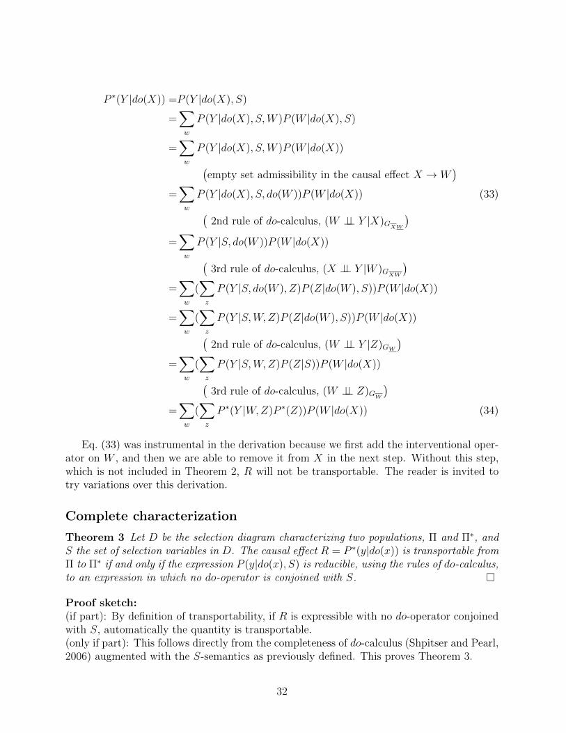
X Z W V Y

Figure 8: Selection diagram demonstrating the incompleteness of Theorem 2.

Appendix 4

Incompleteness of theorem 2

Figure 8 presents an example in which the relation R = P ∗(Y |do(X)) is transportable usingthe criterion of Lemma 1 and, yet, Theorem 2 is too weak to unveil its transportability.

Let us first check case by case the applicability of Theorem 2:

1. R is not trivially transportable (thm. 2/cond. 1) due to confounding X ↔ Z (Tianand Pearl, 2002);

2. There is no S-admissible set (thm. 2/cond. 2) because the confounding V ↔ Y ;

3. There is no set W which make (X ⊥⊥ Y |W ), due to confounding X ↔ Y ;

However, this quantity is still transportable using the do-calculus, as the following deriva-tion shows:

31

P ∗(Y |do(X)) =P (Y |do(X), S)

=∑w

P (Y |do(X), S,W )P (W |do(X), S)

=∑w

P (Y |do(X), S,W )P (W |do(X))(empty set admissibility in the causal effect X → W

)=∑w

P (Y |do(X), S, do(W ))P (W |do(X)) (33)(2nd rule of do-calculus, (W ⊥⊥ Y |X)GXW

)=∑w

P (Y |S, do(W ))P (W |do(X))(3rd rule of do-calculus, (X ⊥⊥ Y |W )GXW

)=∑w

(∑z

P (Y |S, do(W ), Z)P (Z|do(W ), S))P (W |do(X))

=∑w

(∑z

P (Y |S,W,Z)P (Z|do(W ), S))P (W |do(X))(2nd rule of do-calculus, (W ⊥⊥ Y |Z)GW

)=∑w

(∑z

P (Y |S,W,Z)P (Z|S))P (W |do(X))(3rd rule of do-calculus, (W ⊥⊥ Z)GW

)=∑w

(∑z

P ∗(Y |W,Z)P ∗(Z))P (W |do(X)) (34)

Eq. (33) was instrumental in the derivation because we first add the interventional oper-ator on W , and then we are able to remove it from X in the next step. Without this step,which is not included in Theorem 2, R will not be transportable. The reader is invited totry variations over this derivation.

Complete characterization

Theorem 3 Let D be the selection diagram characterizing two populations, Π and Π∗, andS the set of selection variables in D. The causal effect R = P ∗(y|do(x)) is transportable fromΠ to Π∗ if and only if the expression P (y|do(x), S) is reducible, using the rules of do-calculus,to an expression in which no do-operator is conjoined with S. �

Proof sketch:(if part): By definition of transportability, if R is expressible with no do-operator conjoinedwith S, automatically the quantity is transportable.(only if part): This follows directly from the completeness of do-calculus (Shpitser and Pearl,2006) augmented with the S-semantics as previously defined. This proves Theorem 3.

32

Appendix 5

In the next two examples, we show that the definition of mechanism is intrinsically connectedwith the third layer of the causal hierarchy, as defined in (Pearl, 1995, 2009), and to appropri-ately use the theory of transportability qualitative structural knowledge about the problemis needed beyond the knowledge expressed through local interventional distributions.

First example

Consider graph G = {X → Z → Y,X ← U1 → Z,Z ← U2 → Y }, where X is encour-agement to take a drug, Z is taking the drug, Y is recovery, U1 is personal attitude, U2 isgender.

In model 1 (LA population), men are contrarian and cured by drug, when women areobedient and hurt by the drug. In model 2 (NY population), no one is affected by thedrug. Let ⊕ stands for the logical gate exclusive or (XOR). The functional description isgiven by P (U1) = P (U2) = 1/2 equal in both models, and the functions in model 1 are:X = U1, Z = X ⊕ U2, Y = Z ⊕ U2. In model 2, the functions are: X = U1, Z = U2, Y = U2.

We measure local interventional distributions in both populations, and obtain Px(z) =P ′x(z) = 1/2 for all X and Z, and Pz(y) = P ′z(y) = 1/2 for all Z and Y . Now, computingthe non-local interventional distribution Px(y), we notice in LA Px(y) = 1 when y = x, andzero otherwise, but in NY we obtain P ′x(y) = 1/2 for all Y and X.

This demonstrates explicitly that, when we ask whether a certain population differencedeserves an S, we should consider not only differences in ACE but also differences in func-tional relations. In other words, differences in functional relations which do not show asdifferences in local ACE can combine and yield differences in non-local ACE. A definitionin terms of mechanisms f()s and exogenous distributions P (u)s is necessary.

Second example

One definition of mechanism is: a probability distribution Pr over the set of functions frompa(Y ) to Y . (Because the pair Y = f(pa(Y ), U) and P (u) defines such Pr.) But thefollowing example shows that this definition is insufficient.

Consider the same story as in the first example. Now, consider the functional model 1:X = U1, Z = X ⊕ U2, Y = Z ⊕ U2, and model 2: X = U1, Z = X ⊕ U2, Y = Z ⊕ U2, whereU2 is the complement of U2.

In this case we have Pr() = Pr∗(), because the probability assigned to each of the fourfunctions is the same in both models, it is only the labeling on the values of the U2 variablethat is different. Now, let us compare ACE with ACE∗. For ACE we have P (y|do(x)) = 1,if y = x, and 0 otherwise; for ACE∗ we have P (y|do(x)) = 0 if y = x, and 1 otherwise(because Y = (X ⊕ U2)⊕ U2 = X, Y = (X ⊕ U2)⊕ U2 = X).

The moral of the story is that equality of all Pr’s is not sufficient to guarantee equalityof all causal effects – the labeling on the four functions is as important and, hence, it shouldbe part of what we define as “mechanism”. The label can be neglected though when thereis no confounding arc into Y .

33