transport costs and economic growth in a backward … · revista de historia econo´mica, ... 7 in...

TRANSPORT COSTS AND ECONOMIC GROWTH INA BACKWARD ECONOMY: THE CASE OF PERU,1820-1920*

LUIS FELIPE ZEGARRACENTRUM Catolica, Pontificia Universidad Catolica del Peru a

Costos de Transporte y Crecimiento Economico en una Economıa Sub-desarrollada. El Caso del Peru, 1820-1920

ABSTRACT

This paper analyses the system of transportation and discusses the effectof geography and transport infrastructure on transport costs and economicgrowth in Peru during the 19th and early 20th centuries. Using primaryand secondary sources, I find that geography imposed difficult transportchallenges on Peruvians during this period. There were no navigable riversin coastal and highland regions, railroads were scarce and most roads wereinadequate for wagons, sometimes even for horses and mules. As a result,transport costs were extremely high, which constituted a barrier to trade,reduced gains from specialisation and retarded economic growth. Therefore,high transport costs seem to be one important factor in explaining the lowincome levels of Peru in the early 20th century in spite of the country’s largeendowments of natural resources.

Keywords: transportation, railroads, Peru, Latin America

JEL Code: N70, N76, R40

* Received 1 September 2010. Accepted 21 June 2011. I appreciate the comments and suggestionsof the three anonymous referees and am grateful to the staff of the National Library of Peru, theLibrary of the Pontificia Universidad Catolica del Peru and the Library of the Municipality of Lima fortheir help and assistance during the process of data collection.

a Professor of CENTRUM Catolica, The Business School of Pontificia Universidad Catolica delPeru. [email protected]

Revista de Historia Economica, Journal of lberian and Latin American Economic HistoryVol. 29, No. 3: 361–392. doi:10.1017/S0212610911000188 & Instituto Figuerola, Universidad Carlos III de Madrid, 2011.

361

RESUMEN

Este artıculo analiza el sistema de transporte y discute el efecto de lageografıa y de la infraestructura de transporte en los costos de trasporte y elcrecimiento economico en el Peru durante el siglo XIX y principios del sigloXX. Usando fuentes primarias y secundarias, mostramos que la geografıaimpuso dificultades severas a los peruanos durante este perıodo. El Peru notuvo rıos navegables en la costa y en la sierra, hubo pocos ferrocarriles, y lamayor parte de los caminos eran inadecuados para carretas, incluso paracaballos y mulas. Como resultado, los costos de transporte fueron extrema-damente altos, lo que represento una barrera al comercio, redujo lasganancias por especializacion y afecto el crecimiento economico. Por lotanto, los altos costos de transporte parecen ser uno de los factores queexplican los bajos niveles de ingreso de los peruanos a principios del siglo XXa pesar de sus grandes dotaciones de recursos naturales.

Palabras clave: transporte, caminos, Peru, America Latina

1. INTRODUCTION

In a world with gains from specialisation, transport costs may reducethe benefits of trade and retard economic growth1. Gallup et al. (1999), forexample, found that coastal regions and those linked to coasts by ocean-navigable waterways are strongly favoured in development in comparisonwith their hinterlands. Other articles also indicate that geography andtransport costs affect trade and economic growth (Rousslang and To 1993;Eaton and Kortum 2002; Overman et al. 2003).

Historical evidence has been useful for analysing the economic effects oftransport costs and technological innovations in transportation over longperiods of time. In particular, the economic impact of railroads in the 19th

and early 20th centuries has received much attention in the literature. Rostow(1962), for example, indicated that «the introduction of the railroad has beenhistorically the most powerful single initiator of take-offs. It was decisive inthe United States, Germany and Russiay» (Rostow 1962, p. 302). Fremdling(1977), Price (1975) and Metzer (1974) also support the hypothesis thatrailroads played an important role for economic growth in Germany, Franceand Russia, respectively. Fogel (1962, 1964, 1979), however, argues thatpre-rail modes of transportation in the United States were not necessarily

1 Increasing returns and horizontal specialisation, as well as vertical specialisation, may allowus to explain why transport costs reduce trade.

LUIS FELIPE ZEGARRA

362 Revista de Historia Economica, Journal of lberian and Latin American Economic History

associated with high transport costs, and therefore the construction ofrailroads in the 19th century did not yield large social savings2.

In the case of Latin America, historical studies support the hypothesisthat transportation costs were high in the pre-rail era and that the con-struction of railroads led to large social savings. Coatsworth (1979) indicatesthat in Mexico, before the railroad, waterways were not available in thehabitable regions3, and thus freight was transported by wagon or on thebacks of animals and men. The construction of railroads then reduced timeand money transport costs, increasing trade and market integration (Dobadoand Marrero 2005). Similarly, for Brazil, Leff (1972) and Summerhill (2005)indicate that prior to the construction of railroads, waterways were notwidely used for transportation and the conditions of the terrain were poor4.As a result, transport costs from the agricultural regions to the largestmarkets were high. In addition, McGreevey (1971) and Hoernel (1976) alsoindicate that railroads played an important role in reducing transport costsand promoting economic growth in Colombia and Cuba, respectively.

Overall, it seems that prior to railroads, the availability of waterwaysprovided a low cost mode of transportation. Transportation in wagons or onthe backs of animals and men was more expensive. The impact of railroadson transport costs depended on the existence of waterways: if waterwayswere not available, the impact of railroads on transportation costs was large.

For Peru, some studies have analysed the role of transportation costs inthe mining sector in the Central Andes and the interaction between therailroad and the traditional system of mules and llamas. According to Miller(1976), railroads played an important role for the mining sector in the centralhighlands of Peru but yielded small effects in other sectors, in particularagriculture. More recently, Contreras (2004) and Deustua (2009) also indi-cated that the construction of railroads facilitated the expansion of miningproduction, especially copper, in the Central Andes5.

2 Fishlow (1965), Hawke (1970) and Vamplew (1971) also support the idea that the social savingsof railroads in the United States and some European countries were not very large. Similarly, Craftsand Mulatu (2006) indicate that falling transport costs before World War I had no major effect on thelocation of industry in Great Britain.

3 Coatsworth (1979) indicates that Mexico did not have a river system suitable for use intransportation, and that most of the population and economic activity was located too far from thetwo coasts to use the sea as a means of communication.

4 Leff, for example, indicates that «Brazil’s large hinterland did not have an extensive networkof navigable waterways in the habitable areas comparable to the Mississippi and Great Lakessystems in the United States. Man-made transportation facilities were also noticeably lacking.» Leff(1972, p. 490). More recently, Summerhill (2005) also indicates that Brazil was deficient in transportfacilities prior to the construction of railroads, with the exception of settlements near to the coast.Social savings from railroads were then large. In addition, unlike Summerhill (2005), Mattoon(1977) indicates that road conditions in Sao Paulo in the 19th century were totally inadequate.

5 These studies indeed represent a contribution to understanding the impact of transport costson the Peruvian economy. However, the literature lacks formal testing of the impact of transportinnovations on economic growth.

TRANSPORT COSTS AND ECONOMIC GROWTH IN A BACKWARD ECONOMY

Revista de Historia Economica, Journal of lberian and Latin American Economic History 363

In this article, I examine the system of transportation in the 19th and early20th centuries in Peru and analyse the effect of geography and transport infra-structure on transport costs, trade and economic growth during this period.The main objective of this study is to explore to what extent the transportationsystem of Peru contributed to the slow growth of the Peruvian economy duringthis period. This article is one of the few studies on the history of transportationin Peru and may help to understand the impact of geography and transportinfrastructure on economic growth in a backward economy.

The study of transportation in Peru for this period is crucial for explainingthe sluggish record of economic growth of this country. Peru is a special case,because it had a poor economic performance in spite of its favourable factorendowments. Contemporary observers described the abundance of naturalresources, especially agricultural and mineral (Ledesma and Bollaert 1856;Markham 1874). In spite of the abundance of natural resources, in the early20th century, income levels of Peruvians were among the lowest in the region.High transport costs may constitute one possible explanation for the sluggisheconomic performance of Peru during this period.

The structure of the paper is as follows: Section 2 describes the geo-graphy, transport infrastructure and modes of transportation in the 19th andearly 20th centuries. Section 3 reports some estimates on freight rates forusing roads, railroads and the sea. Section 4 reports some estimates on timecosts for the different modes of transportation. Section 5 discusses thepossible effects of transportation costs on trade and economic growth inPeru during this period. Section 6 concludes the paper.

2. ROADS, RAILROADS AND WATERWAYS

In this section, I will provide an overview of the geography, transportinfrastructure and modes of transportation of Peru during the 19th and early20th centuries. As I will show, geography and the lack of infrastructureimposed severe obstacles to transportation during this period.

On the coast, geography and weather generated great challenges fortransportation. The coast was largely constituted by large plains of sand6,which made the traction of wheels and even the work of horses and mulesvery difficult. These difficulties made journeys seem longer than they were7.Moreover, the heat in the desert could be deadly for the traveller and hishorse, which meant that travellers preferred to travel at night in order toavoid the heat, although they ran the risk of straying off course when there

6 Stevenson (1825) indicates that the Lima–Trujillo route in the north of Peru was 108 leagues(around 370 miles), of which 88 leagues were sandy (Stevenson 1825, p. 113, Vol. II).

7 In 1873, for example, Raimondi indicated that the distance between Pativilca and Huarmeyon the northern coast of Peru was 16 leagues, but most people thought it was 25 leagues (Raimondi2006, p. 114).

LUIS FELIPE ZEGARRA


was no moonlight8. Freight was carried in wagons or directly on the backs ofhorses and mules (Deustua 2009). Horses were faster than mules in regularconditions. However, in the extreme conditions of the sandy, dry Peruviandeserts, mules were probably better than horses9. Even on the Lima–Callaoroute, traffic was «unthinkable without mule trains» (Waszkis 1993, p. 137).

The sea became an alternative means of transportation for coastal towns.With the introduction of steam navigation in the 1840s, travel along the coastwas not affected by ocean currents and wind, and travellers enjoyed a fasterand safer mode of transportation10. Coastal towns could then engage in tradeby using the sea as a means of transportation. However, navigation facedsome difficulties. For instance, with the exception of Callao, the main Peruvianport, the other coastal ports lacked proper installations to facilitate trade: theywere simply natural ports (Contreras 2004)11.

In the highlands, geography and inadequate transport infrastructure madetransportation even more difficult than on the coast12. Long, steep ascents,deep canyons, almost vertical hillsides and narrow roads made transportation

8 Tschudi (1847) considered transportation along the Peruvian coast as difficult, tedious anddangerous. In his words, «the roads lead through plains of sand, where often not a trace of vege-tation is to be seen, or a drop of water to be found for twenty or thirty miles. It is found desirable totake all possible advantage of the night, in order to escape the scorching rays of a tropical sun; butwhen there is no moonlight, and above all, when clouds of mist obscure the directing stars, thetraveler runs the risk of getting out of his course, and at daybreak, discovering his error, he mayhave to retrace his weary way. This extra fatigue may possibly disable his horse, so that the animalcannot proceed further. In such an emergency a traveler finds his life in jeopardy; for should heattempt to go forward on foot he may, in all probability, fall a sacrifice to fatigue and thirst»(Tschudi 1847, p. 138).

9 The mule was the «camel of the desert»: the endurance of mules when tired and with limitedfood supplies was extraordinary (Tschudi 1847, pp. 205-206).

10 «Even in sailing vessels voyages from south to north can be conveniently performed inconsequence of the regularity of the trade wind.» (Tschudi 1847, p. 207).

11 In 1826 Callao was one of the few ports with proper installations for disembarking (Denegri1976). In the 1920s, one century later, most coastal ports still lacked proper infrastructures. Jones(1927) indicated that out of the approximately thirty Peruvian seaports, only nine major portshandled exports and imports, and only four had fair harbors. Most ports only had «y open road-steads unprotected from the winds and the ocean swell. As a result steamers usually anchora mile or more off shore, and discharge or receive freight and passengers by means of lighters andlaunches, a slow and rather inefficient means of transfer» (Jones 1927, p. 24).

12 De Tschudi (1847) indicates that «all roads running from the coast to the Sierra, present asimilarity of character. Taking an oblique direction from the margin of the coast, they run into oneor other of the fan-shaped Cordillera valleys, all of which are intersected by rivers. Following thecourse of these rivers, the roads become steeper and steeper, and the valleys soon contract into mereravines, terminating at the foot of the Cordillera y» (Tschudi 1847, p. 255). In addition, in bothcoastal and highland regions, roads did not follow straight lines. The absence of bridges in someregions increased distances, since a traveller had to ride longer distances to find a safe way ofcrossing a river. For example, Raimondi indicated that although the distance in a straight linebetween the hacienda Pucala and Patapo in the north of Peru is only one and a half leagues, thepresence of rivers and the lack of roads made it necessary to complete 5 leagues (Gomez and Bazan1989). In addition, roads going around mountains also went up and down. Davalos y Lisson (1919)indicates that roads that in a straight line were 100 kilometers long and had slopes of 3-6 per cent,ended up being 120 or 140 kilometers long with gradients of even 30 per cent.



very difficult and almost impeded the use of the wheel. In the 1890s, ErnstMiddenford observed that the geography of the Andes was never as complexas in Peru. The terrain was rarely flat, with the exception of the plateau ofTiticaca and the valleys of Jauja and Vilcanota in the most populated regions(Middenford 1974, p. 10, Vol. III). Deep precipices and narrow roads madetravel very dangerous. Roads were, in fact, so narrow that in some places twomules could not pass at the same time. In addition, during the rainy season(December-April), communication could be completely halted13.

In the highlands, freight was carried on the backs of mules and llamas.Mules had some advantages and disadvantages in comparison to llamas. Oneof the advantages of mules is that they could carry up to 300 pounds, whereasllamas could not carry more than 125 pounds, and even 100 pounds wasusually considered a full load (Hills 1860, p. 101). Mules were then moreappropriate for carrying heavy items. In addition, mules were faster thanllamas: mules could cover as many as 35 miles per day, whereas llamas couldonly manage 15 miles at the most. Finally, mules could stand the heat of thecoastal desert, whereas llamas could not. For journeys to or from the coast,then, mules were required for at least part of the route. On the other hand,llamas were better suited than mules for the difficult terrain and weather ofthe Andes14, and did not require much care since they were mostly fed fromany herbage, which lowered their maintenance costs (Cisneros 1906, p. 124).

As a result of the differences between mules and llamas, mules werebetter for transporting heavy cargo on long journeys. Llamas were better fortransporting smaller amounts of freight on short journeys in the highlands.In mining, for example, prior to the construction of the Central Railway,llamas were better for transporting minerals from a large number of mines inthe Central Andes to the main mining haciendas where the minerals were

13 In addition, from May to November, banditry could also interrupt communication(Contreras 2004, pp. 76-77). Testimonies of travellers are quite illustrative. For instance, Wortley(1851) described the roads between the coast and the highland and indicated that «y the elevatedplateau and table-lands, separated by deeply-embosomed valleys, and the gigantic mountains thatintervene between the coast and the table-land, render travelling tedious and difficult. Roads andbridges, in many parts, are entirely wanting; and in places where rude and scarcely-distinguishablepaths are found, they lie along the perilous edges of overhanging and rugged precipices, perpen-dicularly steep; and these tracks, moreover, are almost always so dangerously narrow, that the sure-footed mule can alone tread them with any security y» (Wortley 1851, pp. 244-245, Vol. III). Othertravellers also indicated that roads in the highlands made the journey dangerous and exhausting.Consider, for example, Manuel Pardo’s journey from Lima to Jauja in the 1850s (Essay «Estudiossobre Jauja», published as part of the book by McEvoy 2004, pp. 98-99), and Stevenson’s journeyfrom Lima to Cajatambo in the 1820s (Stevenson 1825, pp. 24-26, Vol. II).

14 Contemporary travellers were aware of these differences between mules and llamas. Hills(1860), for example, indicated that a llama «has spongy hoofs and claws, which enables him to passover beds of ice with ease, and is well protected by his fleece from any cold to which he may beexposed» (Hills 1860, p. 101). Moreover, Cisneros (1906) observed that llamas could live in placeswhere mules would die of hunger and cold. In addition, Tschudi (1847) pointed out that llamascould carry freight from places where the slopes were so «steep that neither asses nor mules cankeep their footing» (Tschudi 1847, p. 308).

LUIS FELIPE ZEGARRA


concentrated, whereas mules were used for transporting minerals from thosehaciendas to Callao. On the coast, mules had to be used for even shortjourneys because llamas could not stand the heat in the sandy deserts.

One important drawback of Peru’s topography is that rivers were notnavigable in the habitable regions. Rivers flowed from the highlands to thePacific coast, but they were not appropriate for navigation. Navigable riversexisted only in the jungle, which was mostly uninhabited15. Jones (1927)indicated that the lack of navigable rivers imposed enormous trade handi-caps. «y No large navigable rivers offer routes into the interior and othermeans of entering the mountain zone are not easily provided16.»

Peruvians could also use railroads for transportation from the mid-19th

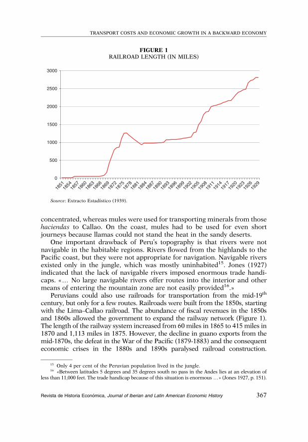
century, but only for a few routes. Railroads were built from the 1850s, startingwith the Lima–Callao railroad. The abundance of fiscal revenues in the 1850sand 1860s allowed the government to expand the railway network (Figure 1).The length of the railway system increased from 60 miles in 1865 to 415 miles in1870 and 1,113 miles in 1875. However, the decline in guano exports from themid-1870s, the defeat in the War of the Pacific (1879-1883) and the consequenteconomic crises in the 1880s and 1890s paralysed railroad construction.

FIGURE 1RAILROAD LENGTH (IN MILES)

0

185118541857186018631866186918721875187818811884188718901893189618991902

19081911191419171920192319261929

1905

500

1000

1500

2000

2500

3000

Source: Extracto Estadıstico (1939).

15 Only 4 per cent of the Peruvian population lived in the jungle.16 «Between latitudes 5 degrees and 35 degrees south no pass in the Andes lies at an elevation of

less than 11,000 feet. The trade handicap because of this situation is enormous y» (Jones 1927, p. 151).



The length of the railway system actually declined to 937 miles in 1883 and thenincreased to only 993 miles in 1890 and 1,118 miles in 1900.

A large number of towns were not connected by railroads in the early 20th

century (Figure 2). Davalos y Lisson (1919) indicated that, according to a studyby the engineer Tizon y Bueno, in the 1910s there were around 10,000 towns inPeru and that only 300 of them were connected by railroad. Similarly, Milstead(1928) indicated that railroad infrastructure was very deficient not only in thehighlands, but also on the coast. According to Milstead, in the early 1920sprimitive transportation facilities persisted in around 85 per cent of the country.Only 2,018 miles of steam railroads and 100 miles of street and interurban lineswere in operation in 1924. Although some railways had been constructed in the1850s, there was no integrated railway network (Milstead 1928, p. 68). Mosttowns depended largely on the traditional system of mules and llamas.

A comparison with other countries indicates that Peru had a relativelylow level of railway coverage. In 1913, Peru only had 0.7 miles of railwaytrack per 1,000 inhabitants. In contrast, the corresponding figure forArgentina was 4.3 miles. Other countries with at least 1 mile of railway trackper 1,000 inhabitants were Brazil, Chile, Costa Rica, Cuba, Mexico, Panamaand Uruguay17.

Therefore, geography and the lack of proper transport infrastructureimposed challenges on Peruvians in the 19th and early 20th centuries.Transportation along the coast and in the highlands was a difficult task.Several sources largely agree on the difficulties of travelling in the aridsandy desert or the steep Andes Mountains, and on the lack of proper portinstallations and of navigable rivers in the habitable regions. The construc-tion of railroads, which started in the mid-19th century, probably madetransportation faster and less costly. However, by the early 20th century onlya few miles had been built. In these circumstances, time and money trans-port costs for most Peruvians must have been high.

3. FREIGHT RATES

This section reports some estimates of freight rates for overland and seatransportation18. As indicated previously, the geography and transportinfrastructure in Peru imposed some difficulties on transportation. Freightrates, then, must have been high19.

17 These figures are from Bulmer-Thomas (2003)18 All figures are in 1,900 soles. The sol was the Peruvian currency from 1863. Prior to 1863,

Peruvians used the peso. However, the specie content of the peso was the same as the specie contentof the sol. Since prices varied over this period, I deflacted freight rates using a price index. Thesources for the price index are from Gootenberg (1990) and Quiroz (1993).

19 This section only deals with freight rates. However, data on passenger fares yield similarconclusions: the traditional system of animal transportation was more costly than steam ships andrailroads.

LUIS FELIPE ZEGARRA


FIGURE 2MAP OF RAILROADS IN PERU, 1930

Source: Deustua (2010, p. 191).



Let us start with the analysis of the traditional system of animal trans-portation. Table 1 reports freight rates for using mules and llamas. There wasgreat disparity in freight rates between different routes, regions and dates.However, it is possible to locate some patterns that will allow us to identifysome of the determinants of freight rates.

First of all, some of the differences in freight rates were due to thedifferences in the demand for mules and llamas. The importance of demandseems high when looking at the evolution of freight rates. As the need fortransportation increased, freight rates increased. According to Miller (1976), forexample, as the production of copper started to boom in the central highlands inthe late 1890s, the demand for transporting copper, therefore, increased andthe price of transportation increased substantially. The cost of renting a mule(in constant 1,900 soles per tonne) for the Cerro de Pasco–La Oroya routeincreased from 21 soles in 1896 to 104 soles in 1898, although it then declined to70 soles in 1900. Over the same period, the cost of renting a llama rose fourfold(Miller 1976). Freight rates were high in 1900 not only for Cerro–La Oroya butalso for other mining routes, such as Cerro de Pasco–Goyllarisquizga and Cerrode Pasco–Yanahuanca. Contreras (2004) indicates that some attempts to reducetransport costs were made, but they were not successful. In 1899, a transpor-tation company and miners reached an agreement to charge 53 current solesfor transporting minerals from Cerro de Pasco to La Oroya. The company hiredarrieros and provided the service to miners. However, this agreement wassoon broken because of the scarcity of men. The company did not find arrierosto transport the mineral, requesting miners to bring their own men. Arrieros’salaries and the consequent cost of transportation then increased.

In other regions, freight rates also increased in response to the increasingdemand for transportation. The increase in coffee production in Junin, forexample, led to an increase in the price of transportation. According to themunicipality of Chanchamayo, freight rates by mule between La Oroya andLa Merced increased from 30 constant soles in 1894 to 52 constant soles in1895 (Pinto and Salinas 2009, p. 130).

On the other hand, the construction of railroads increased the supply oftransportation and led to a reduction in freight rates. For instance, on the LaOroya–Huancayo route mule freight rates declined from 80 constant soles in1900 to only 28 constant soles in 1906. Furthermore, with the construction ofrailroads, the demand for mules and llamas declined in nearby regions, andthus the cost of renting these animals declined.

In addition, rates depended on the difficulty of the journey. In particular, theprice of transportation was greater on uphill routes than on downhill journeys,because the depreciation of the animal was greater in the case of the former.For the Huarochiri–Chicla route, for example, Deustua (2009) indicates that inthe late 1880s the price of transportation by mule was 19.8 constant soles onuphill routes and 17.8 soles per tonne downhill, whereas the correspondingfreight rates by llama were 5.9 soles and 4.5 soles per tonne.

LUIS FELIPE ZEGARRA


TABLE 1FREIGHT RATES OF THE TRADITIONAL SYSTEM OF OVERLAND TRANSPORTATION

1,900 soles

Route Region1 YearDistance(miles)

Cost pertonne

Cost pertonne-mile Source

Mule transportation/1830-1870

Cerro de Pasco–Lima C/H 1836 204 57.2 0.28 Deustua (2009)

Lima–Callao C 1860 9 3.8 0.44 McEvoy (2004)

Jauja–Lima C/H 1860 156 63.3 0.41 McEvoy (2004)

Islay–Arequipa C 1856 104 32.0 0.31 Bonilla (1976)

Islay–Arequipa C 1862 104 38.3 0.37 Bonilla (1976)

Arequipa–Puno H 1860s 184 35.1 0.19 Flores (1993)

Arequipa–Cuzco H 1860s 415 105.4 0.25 Flores (1993)

Mule transportation/1880-1920

Highlands2 H 1909 0.42 Tizon (1909)

Cerro de Pasco–Callao C/H 1890 196 178.6 0.91 Miller (1976)

Cerro de Pasco–La Oroya H 1896 83 21.1 0.25 Miller (1976)



Cerro de Pasco–Casapalca H 1897 112 37.1 0.33 Miller (1976)

Cerro de Pasco–Goyllarisquizga H 1900 22 33.0 1.48 Miller (1976)

Cerro de Pasco–Yanahuanca H 1900 29 24.0 0.84 Miller (1976)

La Merced–Tarma H 1886 48 52.3 1.09 Pinto and Salinas (2009)

La Merced–La Oroya H/J 1894 79 29.7 0.38 Pinto and Salinas (2009)

La Merced–La Oroya H/J 1895 79 51.5 0.65 Pinto and Salinas (2009)

Huarochiri–Chicla (down) H 1889 19 17.8 0.96 Deustua (2009)

TR

AN

SP

OR

TC

OS

TS

AN

DE

CO

NO

MIC

GR

OW

TH

INA

BA

CK

WA

RD

EC

ON

OM

Y

Revis

tade

His

toria

Econom

ica,

Journ

alof

lberia

nand

Latin

Am

eric

an

Econom

icH

isto

ry371

TABLE 1 (Cont.)

1,900 soles

Route Region1 YearDistance(miles)

Cost pertonne

Cost pertonne-mile Source

Huarochiri–Chicla (up) H 1889 19 19.8 1.06 Deustua (2009)

La Oroya–Huancayo H 1900 96 80.0 0.84 Miller (1976)

La Oroya–Huancayo* H 1906 96 28.0 0.29 Miller (1976)

La Oroya–Perene H 1901 99 74.3 0.75 Miller (1976)

La Oroya–Jauja* H 1906 71 20.3 0.28 Miller (1976)

Jauja–Tarma H 1906 36 12.7 0.35 Miller (1976)

Huancayo–Jauja H 1906 24 11.0 0.45 Miller (1976)

Huancayo–Chanchamayo H 1906 99 50.9 0.51 Miller (1976)

Huancayo–Huancavelica H 1906 68 41.5 0.61 Miller (1976)

Huancayo–Ayacucho H 1906 160 92.4 0.58 Miller (1976)

Ayacucho–Pisco C/H 1909 186 108.2 0.58 Tizon (1909)

Llama transportation

Huarochiri–Chicla (down) H 1889 19 4.5 0.24 Deustua (2009)

Huarochiri–Chicla (up) H 1889 19 5.9 0.32 Deustua (2009)

Parac–Chicla H 1893 17 4.7 0.27 Deustua (2009)

Parac–San Mateo H 1893 10 4.7 0.45 Deustua (2009)

Elisa (mine)–Casapalca H 1892 5 2.8 0.57 Deustua (2009)

Highlands2 H 1909 173 36.1 0.21 Tizon (1909)

Notes: Freight rates are in 1,900 soles.1C: coast, H: highlands, J: jungle.2Tizon (1909) reports freight-rate figures for a distance of 50 leagues in the highlands for mules and llamas. Tizon does not specify a route.*A railway competed with mule transport for the whole of part of the route.

LU

ISF

EL

IPE

ZE

GA

RR

A

372R

evis

tade

His

toria

Econom

ica,

Journ

alof

lberia

nand

Latin

Am

eric

an

Econom

icH

isto

ry

Finally, llama freight rates were usually cheaper than mule rates. Llamarates were usually lower than 0.5 soles per tonne-mile, whereas mule rateswere usually higher than 0.5 soles per tonne-mile, and in some cases theywere more than 1 sol per tonne-mile20. The lower cost of using llamas is notsurprising considering that these animals did not require much care, sincethey mostly fed upon practically all species of herbage from the mountains,and were better suited than mules to the natural conditions of the Andes(Hills 1860, p. 101). In addition, by the mid-19th century, the price of astrong, fully grown llama ranged between 3 and 4 soles, and a regular llamacould be purchased for 2 soles (Tschudi 1847, p. 308); however, the priceof a regular mule ranged between 45 and 50 soles, and could reach up to250 soles (Deustua 2009, pp. 176-177).

A comparison with other modes of transportation indicates that thetraditional system of animal transportation was very costly, especially as theneeds for transportation increased at the turn of the century. Let us considerthe freight rates charged by railroads, a more time efficient mode of trans-portation. Table 2 reports the effective freight rates for a number of routes forthree types of freight21. First class referred to imported goods, second class tomanufacturing goods and third class to mining and agricultural products.

If we compare mule and railroad rates, we find that effective freight rateswere usually lower for railroads than for mules, especially on long routes.According to Tizon (1909), transporting loads by mule cost around 0.42 solesper tonne-mile in the highlands. This rate was higher than third-classeffective freight rates for most railroads, and was higher than second-classrates for railroad journeys of more than 10 miles. Since mineral andagricultural products were transported in third-class wagons, transportingthese products by railroad was cheaper than transporting by mule. Otherestimates indicate higher freight rates for mules. The cost of renting a mulefor carrying freight was around 1 sol by 1900 on the La Oroya–Cerro dePasco route. This rate was higher than railroad rates in the Central Railwayon the Callao–La Oroya–Cerro de Pasco route, even in first class.

Consider the composition of production costs of copper, includingextraction, concentration and transportation from Cerro de Pasco to Europe22.Transportation by animals from Cerro de Pasco to La Oroya accounted for35 per cent of total cost, whereas transportation from La Oroya to Callaoaccounted for 11 per cent23. Animal transportation was then much more costlythan railroad transportation. The cost of transporting copper from Cerro de

20 Tizon (1909) indicated that llama rates in the highlands were half mule rates.21 Effective freight rates include terminal fees.22 In 1900, the total cost of transporting copper from Cerro de Pasco to La Oroya by mule and

llama was 836,000 current soles, and the cost of transporting the same mineral from La Oroya toCallao by the Central Railway was only 262,000 current soles. This information is reported byGarland (1901).

23 Extraction and concentration represented only 6 per cent of total cost.



Pasco to La Oroya was around three times the cost of transporting the sameamount of mineral from La Oroya to Callao, even though the distance wasmuch shorter: the distance between Cerro de Pasco and La Oroya was 82 miles,whereas the distance between La Oroya and Callao was almost 140 miles.

On the other hand, traditionally, the transportation of light loads for shortdistances was conducted on the backs of llamas. Compared to railroads,

TABLE 2RAILROADS OF PERU: FREIGHT RATES PER METRIC TONNE (1,900 SOLES), 1908

First classa Second class Third class

RailroadDistance(miles)

(solesper

tonne)

(solesper

tonne-mile)

(solesper

tonne)

(solesper

tonne-mile)

(solesper

tonne)

(solesper

tonne-mile)

Paita–Piura 60 12.28 0.20 9.83 0.16 8.18 0.14

Eten–Chiclayo–Patapo 31 11.70 0.38 10.03 0.32 8.36 0.27

Pacasmayo–Guadalupe 26 10.59 0.41 9.05 0.35 7.50 0.29

Pacasmayo–Yonan 40 13.96 0.35 12.04 0.30 10.12 0.25

Salaverry–Trujillo–Ascope 47 15.62 0.33 13.52 0.29 10.14 0.21

Chimbote–Tablones 35 12.75 0.36 10.95 0.31 9.20 0.26

Supe–Tambo Viejo 7 5.96 0.80 4.93 0.66 3.90 0.52

Lima–Callao 9 7.84 0.92 0.00 0.00 0.00 0.00

Lima–Chorrillos 9 8.34 0.96 0.00 0.00 0.00 0.00

Callao–La Oroya 138 33.76 0.24 29.24 0.21 24.80 0.18

Lima–Ancon 24 8.68 0.37 7.26 0.31 5.84 0.25

Callao–La Oroya–Cerro dePasco

220 55.90 0.25 49.16 0.22 41.41 0.19

Callao–Ticlio–Morococha 115 40.66 0.35 35.25 0.31 29.99 0.26

Tambo de Mora–Chincha 7 5.35 0.72 4.32 0.58 3.29 0.44

Mollendo–Arequipa 107 20.92 0.20 17.58 0.16 13.39 0.13

Mollendo–Puno 325 56.15 0.17 46.93 0.14 36.88 0.11

Mollendo–Sicuani 419 71.41 0.17 59.51 0.14 47.02 0.11

Mollendo–Ensenada–Pampa Blanca

18 0.00 0.00 0.00 0.00 0.00 0.00

Notes and sources: The sources are Costa y Laurent (1908) and Galessio (2007).Data are not available for Lima–Magdalena and for Pisco–Ica.aIn the cases of Lima–Callao and Lima–Chorrillos (1908), freight rates are the only rates available.

LUIS FELIPE ZEGARRA


llamas were much slower, but were not necessarily cheaper, especially as thedemand for transportation increased. Tizon (1909) indicates that llama rateswere around 0.21 constant soles per tonne-mile in 1900 prices. For the 1890s,Deustua (2009) indicates that llameros charged even more than 0.40 soles pertonne-mile. Third-class freight rates by railroad were not necessarily higherthan llama rates. For example, the freight rate for third class by railroad onthe Callao–Cerro de Pasco route was 0.19 soles per tonne-mile, whereas thefreight rate between Callao and Morococha was 0.26 soles per tonne-mile24.

Motivated by the high transport costs of the traditional system of mules(in time costs and freight rates) and llamas (especially in time costs), severalminers supported the construction of the Central Railway. As Contreras(2004) argues, once the railroad reached La Oroya, there were severalattempts to extend the line to Cerro de Pasco. Backus y Johnston and ErnestThorndike obtained permission to conclude the railroad to Cerro de Pasco.On the northern coast, sugar and cotton hacendados also supported andfunded the construction of railroads.

The railroad led to a decline in freight rates. Nevertheless, the reductionin freight rates due to the railroad in Peru was much lower than in otherLatin American countries. On average, the rail freight rate in Peru wasaround 0.16 soles per tonne-mile in 1900 prices. On the basis of the sample offreight rates reported in Table 1, mule freight rates were on average around2.5 times the average rail freight rate and were always lower than five timesthe average freight rate, whereas the rate in the case of llamas was less thantwice the average rail rate25. These differences in freight rates in Perubetween railroads and the alternative system of overland transportation werenot as large as in Mexico and Brazil. In these two countries, wagons were thebest alternative mode of transportation. In Brazil, wagons charged between7.5 and 14.3 times the average rail freight rate; in Mexico, wagons chargedbetween 5.1 and 10.5 times the average rail rate. The construction of rail-roads in Peru, then, reduced freight rates, but not to the same extent as it didin Mexico and Brazil26.

24 According to Miller (1976), around one-third of mining production from Cerro de Pasco wastaken to Callao by llama in 1890, even though it was possible to take it by railroad. This referencehas been taken from Deustua (2009). The lower cost for using llamas is not surprising consideringthat llamas did not require much care, since they mostly fed upon practically all species of herbagefrom the mountains and were better suited than mules to the natural conditions of the Andes (Hills1860, p. 101).

25 These figures were calculated using the freight rates reported by Coatsworth (1979) andSummerhill (2005). These differences in rates may have implied private gains for some firms thatwere served by the railroad and therefore paid less for transportation.

26 One possible explanation for the lower reduction in freight rates due to the railroad was theruggedness of the Peruvian landscape, which led to high operating costs and high rail freight rates;compare, for example, Peru and Brazil. On average, the rail freight rate was U.S.$0.09 per tonne-mile in Peru, almost twice as much as in Brazil. The evidence suggests that these differences infreight rates were due to differences in operating costs. In fact, the gross revenues/operating costsratio was the same in Peru and Brazil: the ratio was 1.54 in both countries (1,904 for Peru and 1,913



Considering the lack of railroads, the sea was an important meansof communication between coastal towns. Table 3 reports data on steamfreight rates for 1876 in 1,900 soles. Total transportation cost includedshipping rates and port fees27. Freight rates ranged between 0.01 and 0.09constant soles per tonne-mile. The figures suggest the presence of scaleeconomies on distance to a large extent for the high cost of using ports:freight rates were lower for longer distances. The distance between the portsof Callao and Tambo de Mora, for example, was only 135 miles and thefreight rate was above 0.08 constant soles per tonne-mile. In contrast, thedistance between the ports of Callao and Puerto Pizarro was 793 miles andthe freight rate was 0.016 constant soles per tonne-mile. Similarly, the dis-tance between the ports of Callao and Arica was 711 miles and the freightrate was less than 0.03 constant soles per tonne-mile. These figures indicatethat the sea as a means of transportation was far cheaper than mules orllamas, especially for long distances28. The sea, however, could not replace

TABLE 3OCEAN FREIGHT RATES, 1876

Freight rate (1900 prices)

Distance (miles) (soles per tonne) (soles per tonne-mile)

Callao–Puerto Pizarro 793 9.67 0.0122

Callao–Paita 626 9.02 0.0144

Callao–Tambo de Mora 135 9.02 0.0670

Callao–Chala 326 11.62 0.0357

Callao–Quilca 518 12.92 0.0250

Callao–Islay 548 12.92 0.0236

Callao–Ilo 618 12.92 0.0209

Callao–Arica 711 12.92 0.0182

Sources: Lemale (1876), Briceno y Salinas (1927) and Bonilla (1976).

(F’note continued)

for Brazil). The higher rail freight rates in Peru seem to be caused by higher operating costs, ratherthan a higher profit margin.

27 Steam freight rates refer to the Pacific Steam Navigation Co. Port fees in Callao, which weresignificant, were included in the freight rates. A British council in Islay indicated in 1862 that thetotal port cost was more than 8 pesos per tonne for using this port. This cost is added to shippingfreight rates to estimate the total cost of transportation.

28 According to Deustua (2009), for example, the merchant Patrico Ginez used mules andhorses to transport goods along the coast; but his favoured means of transportation was the sea(Deustua 2009, p. 177).

LUIS FELIPE ZEGARRA


animal transportation as it faced a natural limitation: it could only be usedfor transporting goods along the coast.

This survey of freight rates shows that the price of transportation for usingmules was greater than the price for using the railroad and steam navigation,especially as the needs for transportation increased from the late 1890s.Muleteering was not only a time-inefficient mode of transportation; it was alsorelatively expensive. Llamas provided a cheaper system of transportation thanmules but were much slower than railroads and steam ships and carried muchless than mules. However, railroads were limited and did not reach most of thePeruvian territory, and rivers in coastal and highland regions were notnavigable, and thus mules and llamas constituted the only or the predominantmode of transportation. Finally, although railroads provided a cheaper modeof transportation than mules and llamas, the reduction in freight rates was notas large as in other Latin American countries.

4. SPEED AND TIME COSTS

Time was a valuable asset. The slow transportation of freight reduced themovement of capital and probably reduced investment opportunities. Thus,low-speed modes of transportation may have reduced the incentives to trade,the gains from specialisation and economic growth.

Table 4 reports the average speed of freight transportation for severalroutes. The speed of mules in transporting freight was not always the same,since it depended on the conditions of the road and the topography of theterrain. In 1906, Cisneros indicated that a loaded mule could complete up to4 miles per hour, or 34 miles per day, on a regular road in the highlands.Other sources indicate lower speeds. According to McGregor, mules usuallytook between 9 and 10 days to complete the Lima–Cerro de Pasco route at anaverage of 19 miles per day. According to Vega and Sulca (2005), herds ofmules usually took 9 days to complete the Huamanga–Abancay route in thesouthern highlands at an average speed of 20 miles per day, and took 7 daysto complete the Abancay–Cuzco route at a speed of 16 miles per day.

Llamas were slower than mules. Tschudi (1847) indicates that llamas wereable to cover between 3 and 4 leagues per day, that is, around 12 miles per day.Similarly, Hills (1860) indicates that llamas rarely managed more than 12 or13 miles per day. For Cisneros (1906), llamas could complete up to 16 milesper day. Since llamas were never fed during the night, the llamero had to stopduring the journey to allow the animals to graze (Tschudi 1847, p. 308).

Railroads constituted an alternative mode of transportation from the mid-19th century. Table 5 reports the speed of railroads for a number of routes in1908. Trains were faster than 7 miles per hour, and thus railroads repre-sented a much faster mode of transportation than mules and llamas. In thecentral region, for example, a train only took 11 hours to complete the route



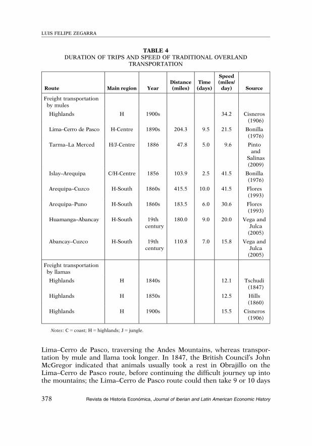
Lima–Cerro de Pasco, traversing the Andes Mountains, whereas transpor-tation by mule and llama took longer. In 1847, the British Council’s JohnMcGregor indicated that animals usually took a rest in Obrajillo on theLima–Cerro de Pasco route, before continuing the difficult journey up intothe mountains; the Lima–Cerro de Pasco route could then take 9 or 10 days

TABLE 4DURATION OF TRIPS AND SPEED OF TRADITIONAL OVERLAND

TRANSPORTATION

Route Main region YearDistance(miles)

Time(days)

Speed(miles/

day) Source

Freight transportationby mules

Highlands H 1900s 34.2 Cisneros(1906)

Lima–Cerro de Pasco H-Centre 1890s 204.3 9.5 21.5 Bonilla(1976)

Tarma–La Merced H/J-Centre 1886 47.8 5.0 9.6 Pintoand

Salinas(2009)

Islay–Arequipa C/H-Centre 1856 103.9 2.5 41.5 Bonilla(1976)

Arequipa–Cuzco H-South 1860s 415.5 10.0 41.5 Flores(1993)

Arequipa–Puno H-South 1860s 183.5 6.0 30.6 Flores(1993)

Huamanga–Abancay H-South 19thcentury

180.0 9.0 20.0 Vega andJulca

(2005)

Abancay–Cuzco H-South 19thcentury

110.8 7.0 15.8 Vega andJulca

(2005)

Freight transportationby llamas

Highlands H 1840s 12.1 Tschudi(1847)

Highlands H 1850s 12.5 Hills(1860)

Highlands H 1900s 15.5 Cisneros(1906)

Notes: C 5 coast; H 5 highlands; J 5 jungle.

LUIS FELIPE ZEGARRA


for muleteers. Deustua (2009) indicates that the railroad took 1 day totransport minerals from Callao to Chicla, whereas herds of mules took 7 or8 days. In the south, the Pisco–Ica railroad completed the 48-mile route in lessthan 4 hours. In contrast, travellers could take nearly a day by horse throughthe desert. On his 1838-1842 trips, J. J. Tschudi completed the journey fromPisco to Ica in 1 day. The journeys were undertaken by horse and through thedesert from 3 pm to the next morning, avoiding the noon heat29.

TABLE 5DURATION OF TRIPS AND SPEED OF RAILROADS

RouteDistance(miles)

Time(hours)

Speed(m.p.h.) Region

North

Piura–Catacaos 7 00:30 13.2 Coast

Pimentel–Chiclayo 9 00:45 11.6 Coast

Eten–Chiclayo–Patapo 26 03:45 7.0 Coast

Pacasmayo–Guadalupe 26 02:45 9.5 Coast

Pacasmayo–Yonan 40 05:00 8.1 Coast

Salaverry–Trujillo–Ascope 47 03:55 12.1 Coast

Center

Chimbote–Tablones 35 03:40 9.7 Coast

Supe–Barranca–TamboViejo

7 00:50 8.9 Coast

Lima–Ancon 24 02:00 11.9 Coast

Lima–Callao 9 00:28 18.3 Coast

Lima–Chorrillos 9 00:28 18.7 Coast

Callao–La Oroya 138 11:45 11.7 Coast/Highlands

La Oroya–Cerro de Pasco 82 06:25 12.8 Highlands

South

Pisco–Ica 46 03:40 12.5 Coast

Tambo de Mora–Chincha 7 00:32 13.9 Coast

Arequipa–Mollendo 107 06:45 15.8 Coast

Arequipa–Puno 218 12:25 17.6 Highlands

Juliaca–Sicuani 123 09:30 12.9 Highlands

Source: Costa y Laurent (1908).

29 The Mollendo–Arequipa–Puno railroad was also much faster than traditional travel methods.The speed of trains on this railroad was above 15 miles per hour. In contrast, in the 1850s S. S. Hills



Therefore, the transportation system of mules and llamas was very slowin comparison to the railway system. Since most of Peru did not have rail-roads, transportation in most regions was relatively slow. Precisely, Davalosy Lisson (1919) indicated that since Peru had not «improved the scarce,narrow and dangerous roads y the social and political life of the nation ismore or less similar to that in the Colony. Towns are isolated some fromthe others. It is not easy for their inhabitants to travel and they never knowthe rest of the nation where they livey The people who are hired fromthe highlands to work for a salary in the haciendas of Pativilca, Casma,Chimbote, Chicama, etc, travel on foot such as during Inca times, needingfrom four to six days to walk distances of no more than 24 to 28 leagues,which would only require eight or ten hours if traveled by railroad or by car»(Davalos y Lisson 1919, p. 371).

Considering the slow construction of railroads and the difficulties oftraditional overland transportation, the sea was an alternative means oftransportation for coastal towns (Table 6). A comparison of navigation andanimal transportation indicates that sailing ships were more time-efficientthan animals when following the Humboldt Current, but yielded about thesame time costs when navigating against the current. The speed of mules wasaround 30 miles a day, whereas that of sailing ships was usually greater than80 miles a day when navigating northward. Steam ships were much fasterthan animals with speeds of above 200 miles a day, and in many casesexceeding 270 miles a day. For instance, a steam ship departing from Callaoand arriving in Huanchaco completed 298 miles per day. Steam ships,therefore, were much more time-efficient than mules and llamas.

In conclusion, the transportation system of mules and llamas was muchslower than railroads and steam ships. Since most routes were completed bythe traditional system of animal transportation (only a few railroads hadbeen built and the sea could only be used to connect coastal towns, whereonly a small proportion of the population lived), the system of transportationof Peru generated high time costs.

5. TRANSPORT COSTS AND ECONOMIC GROWTH

Transportation in most of Peru was conducted by the traditional systemof mules and llamas. Waterways and railroads only served a small portion ofthe territory. Transportation costs were high, which probably constituted abarrier to trade and hindered economic growth. As transport costs were high,

(F’note continued)

travelled from the port of Islay to the city of Arequipa at an average speed of 48 miles per day, fromArequipa to Cuzco at an average speed of 46 miles per day, and from Cuzco to Puno at an averagespeed of 29 miles per day.

LUIS FELIPE ZEGARRA


many towns probably had limitations to participate in trade with othertowns, and thus each town produced what it needed to live. In these cir-cumstances, Peru may have faced severe obstacles to exploit its vast naturalresources. Davalos y Lisson (1919), for example, argues that

«y most mining companies located in Pallasca, Huailas, Cajabamba,Hualgayoc, Cajatambo, Huallanca and some others had experiencedan anemic life because of the lack of means of communication. Thereis nothing richer in Peru in silver, lead, carbon and tungsten thanAncash, or nothing more abundant in gold than Pataz; but since we donot even have horseshoe roads in those provinces, every effort isexhausted for the impossibility of transportation. For the same cause,the great agricultural wealth of Jaen and Maynas has no value.

TABLE 6TIME COSTS AND SPEED OF SAILING AND STEAM SHIPS

Time durationSpeed

(miles per day)

Distance(miles)

Sailingships

Steamships

Sailingships

Steamships

North to South

Paita–Callao 626 15 days 2 days7 hours

41.7 273.2

Huanchaco–Callao 336 7 days 1 day12 hours

48.0 224.0

Callao–Islay 548 18 days 2 days 30.4 273.9

Callao–Arica 711 18 days 3 days 39.5 237.1

Callao–Iquique 838 18 days 3 days12 hours

46.5 239.4

South to North

Callao–Paita 626 6 days 2 days5 hours

104.3 283.5

Callao–Huanchaco 336 4 days 1 day3 hours

84.0 298.7

Islay–Callao 548 4 days12 hours

1 day18 hours

121.7 313.0

Arica–Callao 711 6 days 2 days12 hours

118.5 284.5

Iquique–Callao 838 7 days 3 days 119.7 279.3

Source: Denegri (1976) and Espinosa (2002).



Not even at ten soles per acre can land be sold, not existing roads toreach themy.» Davalos y Lisson (1919, p. 373).

The natural limitations of using animals to transport heavy goods con-stituted a particular constraint to investment and economic growth. Mulescould carry less than 300 pounds, and llamas could carry up to 100 pounds.Heavy machinery, therefore, could not be transported on the backs of mulesand llamas and investment was discouraged. Araoz (1889), for example,argued that the mining business required large concentration plants to reachits «maximum potential». However, the construction of concentration plantsrequired large and heavy machinery, which was practically impossible tocarry on the backs of mules and llamas (Deustua 2009, p. 210).

The lack of modern modes of transportation probably constituted a largera barrier to trade as the demand for transportation increased. When theproduction levels were low, the needs for transportation were also low, andtherefore the system of mules and llamas probably did not represent animportant constraint to investment and economic growth. As more mines wereexploited and more land was cultivated, the needs for transportation increased,and in this situation mules and llamas could not offer the same service as amore modern system of transportation. The scarcity of animals and arrieros ledto the increase in freight rates and represented a significant obstacle totransportation. Nature eventually imposed a constraint on economic growth:the limited numbers of mules, llamas and arrieros were probably not largeenough to support the increasing demand for transportation30.

However, although the comparison of transport costs between the pre-railtransport system, railroads and the sea, as well as the opinion of con-temporary observers, represents valuable information, they do not constituteproof that the system of transportation of Peru represented a significantbarrier to trade and economic growth. A more formal testing procedure isrequired to determine the impact of high transport costs on economicgrowth in Peru. In particular, testing whether the construction of railroadspromoted economic growth may help to understand the economic impact oftransport costs. Considering that transportation in most regions of Peru wasconducted by mule and llama, if the construction of railroads promotedeconomic growth one might argue that the system of transportation in mostof Peru limited the growth of the economy. Using the terminology employed

30 In fact, had railroads not been built in Peru, it would have been physically impossible totransport the same tonnage as was transported by train. Deustua (2009) conducts a simulation toestimate the number of mules needed to replace the Central Railway. In 1890-1900, this railroadcarried almost 104,000 metric tonnes per year. Assuming that mules completed ten round tripsbetween Cerro de Pasco and Callao per year (around 200 days a year), around 100,000 mules wouldhave been required annually during this period only to replace the Central Railway. If each mulecompleted only one round trip, one million mules would have been needed. Deustua indicates thatthis was an «unimaginable scenario» (Deustua 2009, p. 218).

LUIS FELIPE ZEGARRA


by Hausmann et al. (2005), if railroads promoted economic growth, thenthe lack of railroads in most of the country was a «binding constraint» toeconomic growth.

Some might question the validity of the argument that if railroads promotedeconomic growth then the lack of railroads was a binding constraint to eco-nomic growth. It is possible, for example, that only those regions with railroadshad abundant natural resources. In this case, the construction of railroads inregions with no natural resources would not have fostered economic growth.The evidence, however, indicates that Peru had large endowments of naturalresources throughout its territory, and not only in the areas served by railroads.For example, Ledesma and Bollaert (1856) indicated that Peru was

«y one of the richest countries in the world for the animal, vegetableand mineral wealth y Peru produces, in its various climates, all thefruits, grain, and vegetables cultivated in different countries, inde-pendently of those which are indigenous; the latter including many ofexquisite flavor. The transandine region is wonderful for the abun-dance and singularity of its productions. In its immense forests areornamental woods in great variety, together with the Peruvian-barktree, cocoa, coffee, coca, sarsaparilla, vanilla. The mineral kingdom ofPeru is celebrated for placeres of gold and mines of silver, mercury,copper, lead, sulphur, and coal; as well as quarries of various marbles.Important are the gold placers of Carabaya the silver mines of Pasco,Puno, Guantajaya, and Gualgayoc; the mercury mines of Guancavelicaand Chouta; the salt beds of Tarapaca, and the salt pits of Huacho andSechura y» (Ledesma and Bollaert 1856, pp. 217-218)

Similarly, Markham (1874) indicated that the Andes Mountains, «y containinexhaustible stores of copper and silver, the plains afford pasture for largeflocks of alpacas, while the inner slopes of the Eastern Andes produce thebest Peruvian bark, coffee, cocoa, coca, arnotto, and are watered by streamscontaining gold-dust in large quantities» (Markham 1874, p. 127). Peru enjoyedthe presence of abundant natural resources throughout its territory; therefore, itis reasonable to assume that if the railroad played a key role for economicgrowth of the regions it reached it would probably also have had a positiveimpact on the economic growth of other regions.

I use data on exports to estimate the impact of railroads on the economy.The construction of railroads and the consequent reduction in time andmoney transport costs probably led to the growth of market-oriented pro-duction, including production for foreign markets. Not all exports, however,would have been influenced by the construction of railroads to the sameextent. Guano, for example, was extracted from coastal islands and trans-ported directly to Europe by ship. Overland transportation facilities were notrequired for exporting guano. In contrast, crops from the coastal haciendas and



minerals from the highland mines were transported to the sea ports by land,and thus the construction of railroads may have facilitated their transportation.In addition, in the case of mineral exports, Contreras (2004) indicates that theindustry of copper was much more influenced by the construction of theCentral Railway than the silver industry, because of differences in the value/volume ratios. Copper exports tended to have a much lower value/volume ratiothan silver exports, and thus the presence of scale economies in the trans-portation of minerals was larger in the case of copper. On the other hand,considering that the pre-rail costs for transporting crops from the coastalhaciendas to the sea ports were probably lower than the costs for transportingminerals from the mines in the highlands, it is possible that the impact of therailroad was larger for the production of copper in the central highlands thanfor the production of cotton and sugar on the coast.

An econometric approach is used to test whether the length of the railwaynetwork had a significant statistical effect on the level of exports. In parti-cular, the effect of the length of the railway track on the level of exports of thefour main export products (copper, silver, sugar and cotton) in 1920 isestimated, as is the effect of the length of the Central Railway on the volumeof copper and silver exports. The Central Railway connected the port ofCallao, Lima and the mining centres of Junın and Cerro de Pasco and mayhave had a positive impact on the growth of mining exports. The effect ofthe length of coastal railroads on the volume of sugar and cotton exports isalso estimated. Sugar and cotton had been produced mostly on the coastfrom colonial times, and thus the construction of railroads along the coastconnecting haciendas, the main cities and ports may have impacted on thegrowth of cotton and sugar exports.

The following four variables measure the level of exports: COPPER is thenatural log of the copper exports in metric tonnes, SILVER is the natural logof silver exports in metric tonnes, COTTON is the natural log of cottonexports in metric tonnes and SUGAR is the natural log of sugar exports inmetric tonnes31. The following two variables measure the length of railroads:RAIL_CENTRAL is the natural log of the quantity of miles of the CentralRailway and RAIL_COAST is the natural log of the quantity of miles of therailway system in coastal Peru. RAIL_CENTRAL may have a positive effecton SILVER and COPPER, whereas RAIL_COAST may have positive effect onCOTTON and SUGAR.

Let us analyse the time properties of the series. Table 7 reports the statisticsfor the following unit-root tests: Dickey–Fuller, Augmented Dickey–Fuller andPerron. In all tests, the null hypothesis is that the series have unit roots. Thetable also reports the 5 per cent critical values. If the statistics are greater inabsolute value than critical values, then at a 5 per cent significance level thenull hypothesis that the series has a unit root cannot be accepted. In the case

31 Data on exports are taken from Hunt (1973).

LUIS FELIPE ZEGARRA


TABLE 7UNIT ROOT TESTS

Perron

Dickey–Fuller Augmented Dickey–Fuller Zr Zt No. obs.

SILVER

Level 21.851 (22.898) 21.004 (22.899) 25.790 (213.620) 21.550 (22.898) 90

DLevel 212.783 (22.899) 27.591 (22.900) 2113.001 (213.612) 212.952 (22.899) 89

COPPER

Level 22.455 (22.898) 22.336 (22.899) 27.771 (213.620) 22.056 (22.898) 90

DLevel 213.811 (22.899) 211.754 (22.900) 2107.040 (213.612) 215.154 (22.899) 89

SUGAR

Level 20.350 (22.898) 20.051 (22.899) 20.380 (213.620) 20.285 (22.898) 90

DLevel 212.552 (22.899) 25.901 (22.900) 2132.064 (213.612) 212.126 (22.899) 89

COTTON

Level 22.067 (22.898) 21.802 (22.899) 25.036 (213.620) 21.801 (22.898) 90

DLevel 211.222 (22.899) 29.833 (22.900) 292.681 (213.612) 211.735 (22.899) 89

RAIL_CENTRAL

Level 20.690 (22.914) 20.695 (22.915) 21.026 (213.460) 20.662 (22.914) 70

DLevel 28.394 (22.915) 25.992 (22.916) 268.827 (213.452) 28.400 (22.915) 69

RAIL_COAST

Level 21.783 (22.914) 21.801 (22.915) 22.014 (213.460) 21.645 (22.914) 70

DLevel 27.171 (22.915) 23.644 (22.916) 269.996 (213.452) 27.371 (22.915) 69

Notes: The table reports Dickey–Fuller, Augmented Dickey–Fuller (with one lag) and Perron statistics for several models. Null hypothesis is that thevariable has a unit root. 5% critical value are in parenthesis.

TR

AN

SP

OR

TC

OS

TS

AN

DE

CO

NO

MIC

GR

OW

TH

INA

BA

CK

WA

RD

EC

ON

OM

Y

Revis

tade

His

toria

Econom

ica,

Journ

alof

lberia

nand

Latin

Am

eric

an

Econom

icH

isto

ry385

of the series in levels, the statistics are lower in absolute value than the criticalvalues; in the case of the series in differences, the statistics are greater inabsolute value than the critical values. Therefore, all series in our data areintegrated of first-order, or I(1).

The Johansen method is used to test cointegration. If two series arecointegrated, then the Johansen test indicates the existence of at least onecointegrating vector. Table 8 reports the Johansen statistics for the follow-ing hypotheses: there is no cointegrating vector, and there is at least onecointegrating vector. Critical values at a 5 per cent significance level are also

TABLE 8JOHANSEN COINTEGRATION TEST

Rank Null hypothesisLog-

likelihoodTrace

statistic5% critical

value

Variables: SILVER andRAIL-CENTRAL

0 There is nocointegration vector

220.93 10.97 15.41*

1 There is at most onecointegration vector

216.09 1.28 3.76

Variables: COPPER andRAIL-CENTRAL


21.56 5.86 15.41*


21.37 0.00 3.76

Variables: SUGAR andRAIL-COAST


59.79 13.39 15.41*


66.13 0.70 3.76

Variables: COTTON andRAIL-COAST


22.88 6.51 15.41*


26.11 0.06 3.76

Notes: The table reports the statistics for a Johansen cointegration test. All vector-correction modelsinclude ten lags for the endogenous variables in first differences.

*Acceptance of the null hypothesis.

LUIS FELIPE ZEGARRA


reported. I evaluate whether the following pairs of series are cointegrated:COPPER and RAIL-CENTRAL, SILVER and RAIL-CENTRAL, COTTON andRAIL-COAST and SUGAR and RAIL-COAST32. In all cases, at a 5 per centlevel the null hypothesis that the series are not cointegrated cannot berejected. There does not seem to be a long-term relationship between thelevel of exports of the four main Peruvian export products and the length ofthe railway network.

A vector autoregression model for the variables in first differences is thenestimated to determine whether the length of the railroad network promotedthe growth of exports33. Ten lags are included to capture the long-termlagged effects. A Granger test was conducted to determine the causalityrelationship. Table 9 reports the results for the Granger test, and the resultsfor Model 1 indicate that D(RAIL-CENTRAL) caused D(COPPER) andD(COPPER) causes D(RAIL-CENTRAL). A faster growth of railway lengthincreased the growth of copper exports. However, a faster growth of copperexports also promoted the construction of the Central Railway. On the otherhand, the results for Model 2 indicate that the impact of railway constructionon silver exports and vice versa did not seem important. The Granger test

TABLE 9GRANGER TEST OF CAUSALITY

Model Dependent variable Possible cause x2 Probability

Model 1 D(COPPER) D(RAIL-CENTRAL) 27.780 0.002

D(RAIL-CENTRAL) D(COPPER) 32.416 0.000

Model 2 D(SILVER) D(RAIL-CENTRAL) 13.000 0.224

D(RAIL-CENTRAL) D(SILVER) 2.622 0.989

Model 3 D(SUGAR) D(RAIL-COAST) 27.565 0.002

D(RAIL-COAST) D(SUGAR) 116.030 0.000

Model 4 D(COTTON) D(RAIL-COAST) 34.057 0.000

D(RAIL-COAST) D(COTTON) 36.083 0.000

Notes: The table reports Granger statistics and P-values. All vector autoregression models include10 lags for the dependent variables and WAR lagged one year.

32 Ten lags have been chosen in all cases, although the results are similar for other lag speci-fications.

33 D(COPPER) is COPPER in first differences, D(SILVER) is SILVER in first differences,D(SUGAR) is SUGAR in first differences, D(COTTON) is COTTON in first differences, D(RAIL-CENTRAL) is RAIL-CENTRAL in first differences and D(RAIL-COAST) is RAIL-COAST in firstdifferences. I also include a war dummy variable lagged one year to control for the economic effectsof the War of the Pacific (1879-1883).



indicates that D(RAIL_CENTRAL) did not cause D(SILVER) and D(SILVER)did not cause D(RAIL_CENTRAL). The impulse–response functions con-sistently indicate that these variables did not cause each other. Cotton andsugar exports were also influenced by railway length. The results for Model 3indicate that D(SUGAR) and D(RAIL-COAST) also cause each other. Fromthe impulse–response functions, a shock to D(RAIL-COAST) has significanteffects on D(SUGAR) after 3, 5 and 10 years, but a negative effect after 4 years.The results for Model 4 indicate that D(COTTON) and D(RAIL-COAST)caused each other. The impulse–response function indicates that a shockto D(RAIL-COAST) had a positive and statistically significant effect onD(COTTON) after 2 years.

Table 10 simulates the evolution of exports assuming a shock of 1 per centto the railroad length in year t. The table reports the ratio of predictedexports with respect to actual exports for years t 1 5 and t 1 10. I used thecoefficients from the impulse–response functions and calculated the ratiousing the following formula: ytþ k ¼

Qkj¼ 1 ½1 þ yjð1%Þ� for k 5 5, 10, where

yt 1 k is the ratio of predicted exports with respect to actual exports in the yeart 1 k assuming a shock of 1 per cent to the railroad length in year t. Uj is thecoefficient of the impulse–response function and measures the response ofthe natural log of the level of exports (in first differences) to a shock to thenatural log of railroad length (in first differences) after j years. Using thesignificant coefficients from the impulse–response functions, the resultsindicate that copper, sugar and cotton exports responded to shocks to therailroad length. In the case of mining exports, predicted copper exports were

TABLE 10EFFECT OF AN INCREASE OF 1% IN RAILWAY LENGTH ON THE

LEVEL OF EXPORTS

Exports Railroad Period Effect (%)

Copper Central Railway After 5 years 0.00

After 10 years 0.70

Silver Central Railway After 5 years 0.00

After 10 years 0.00

Sugar Coastal Railroads After 5 years 0.85

After 10 years 0.78

Cotton Coastal Railroads After 5 years 0.14

After 10 years 0.14

Notes: The table reports the estimated effect of a 1% shock to the level of railroad length on the level ofexports after 5 and 10 years. The estimates have been obtained using the significant coefficients from theimpulse–response functions.

LUIS FELIPE ZEGARRA


0.7 per cent greater than actual copper exports after 10 years, as a result of ashock of 1 per cent to the length of the Central Railway. However, predictedsilver exports were the same as actual exports: silver exports did not respondto shocks to the length of the Central Railway. In the case of agriculturalexports, sugar and cotton exports responded to railroad construction on thecoast. Predicted sugar exports were greater than actual sugar exports by 0.78per cent after 10 years, whereas predicted cotton exports were 0.14 per centgreater than actual cotton exports also after 10 years.

These results suggest that the construction of railroads had a positiveeffect on the growth of exports. In particular, the railroad promoted theextraction and exportation of copper, cotton and sugar. One implication ofthe econometric results is that if more railroads had been built, the growth ofexports would have been greater during this period. Therefore, as argued byPardo in 1860 (McEvoy 2004), and Davalos y Lisson in 1919 (Davalos yLisson 1919), among several contemporary observers, the absence of low-cost modes of transportation in most of Peru retarded economic growth.

6. CONCLUSIONS

This paper analyses the system of transportation and explores the impact ofgeography and infrastructure on transport costs and economic growth in Peruin the 19th and early 20th centuries. Using primary and secondary sources,I show that geography imposed difficult transport challenges for Peruviansduring this period. The coast imposed high barriers to overland transportationas the sandy desert made travelling difficult and exhausting, whereas thehighlands and their steep, narrow roads made travelling extremely risky andchallenging. In addition, Peru did not have navigable rivers in coastal andhighland regions and most roads were inadequate for wagons.

Railroad construction began in the mid-19th century but was, however, avery slow process. In the early 20th century, Peru was far behind other countriesin the region. On the coast, railroads connected only a few cities and valleys.Only two railway systems linked the coast and the highlands: the CentralRailway, which connected Callao, Lima and the mines of Junin and Pasco; andthe Southern Railway, which ran between Arequipa, Puno and Cuzco. More-over, monopoly power (together with inefficient government regulation) and theabrupt nature of the Peruvian landscape led to high rail freight rates.

Most transportation at the time was conducted on the backs of mules andllamas. This system was associated with high time and money transportcosts, in comparison to railroads and waterways. Freight rates were espe-cially high as the needs for transportation and the demand for mules andllamas increased. For instance, as the production of copper started to boomin the central highlands in the late 1890s, freight rates increased drastically.The scarcity of mules, llamas and arrieros led to significant increases in the



price of transportation. In such circumstances, it seems that the traditionalsystem of overland transportation using mules and llamas represented anobstacle to economic growth.

Employing econometric techniques, I find that the construction of rail-roads promoted the growth of the exporting economy. In the highlands, theconstruction of the Central Railway promoted the growth of copper exports.On the coast, the expansion of the railway system promoted the growth ofsugar and cotton exports. This result is crucial for explaining the slow growthof the Peruvian economy. Since railroads had a positive impact on produc-tion and exports, the lack of railroads in other coastal, highland and jungleregions of Peru probably retarded trade and economic growth. High trans-portation costs were then a binding constraint to growth in most of Peru.

Some might argue that it is not possible to extrapolate the positive role ofrailroads in the copper, sugar and cotton sectors. It is possible that regionswithout railroads did not have other factors that favoured economic growth.In this case, the construction of railroads would have not promoted economicgrowth in those areas, and thus the traditional system of transportation didnot represent a binding constraint to economic growth. Contemporary evi-dence, however, suggests that Peru had other favourable conditions forgrowth. Natural resources, for example, were abundant in other regions. It ispossible then that if railroads had been built throughout the country, thereduction in transport costs would have led to increases in trade, gains fromspecialisation and economic growth.

REFERENCES

ARAOZ, J. (1889): Excursion a Hualgayoc. AUNI, tesis No. 25, May.BONILLA, H. (1976): Gran Bretana y el Peru. Los Mecanismos de un Control Economico.

Lima: Instituto de Estudios Peruanos, Fondo del Libro del Banco Industrial del Peru.BRICENO Y SALINAS, S. (1927): Cuadro General para el Termino de Distancia Judicial, Civil y

Militar dentro de la Republica y aun en el extranjero. Lima: Imprenta Americana.BULMER-THOMAS, V. (2003): The Economic History of Latin America since Independence.

Cambridge: Cambridge University Press.CISNEROS, C. (1906): Resena Economica del Peru. Lima: Imprenta «La Industria».COATSWORTH, J. (1979): «Indispensable Railroads in a Backward Economy: The Case of

Mexico». The Journal of Economic History 39 (4), pp. 939-960.CONTRERAS, C. (2004): El aprendizaje del capitalismo. Estudios de historia economica y

social del Peru Republicano. Lima: IEP.COSTA Y LAURENT, F. (1908): Resena Historica de los Ferrocarriles del Peru. Lima:

Ministerio de Fomento, Litografıa Tip. Carlos Fabbri.CRAFTS, N., and MULATU, A. (2006): «How Did the Location of Industry Respond to Falling

Transport Costs in Britain before World War I?». Journal of Economic History 66 (3),pp. 575-607.

DAVALOS Y LISSON, P. (1919): La Primera Centuria. Lima: Librerıa e Imprenta Gil.DENEGRI, F. (1976): La Republica. Lima: Instituto de Estudios Historico-Marıtimos del Peru.

LUIS FELIPE ZEGARRA


DEUSTUA, J. (2009): El embrujo de la plata. La economıa social de la minerıa en el Peru delsiglo XIX. Lima: BCRP, IEP.

DOBADO, R., and MARRERO, G. (2005): «Corn Market Integration in Porfirian Mexico».Journal of Economic History 65 (1), pp. 103-128.

EATON, J., and KORTUM, S. (2002): «Technology, Geography and Trade». Econometrica70 (5), pp. 1741-1779.

ESPINOSA, C. (2002): «Entre la Ciudad y el Continente: Opciones para la construccion delos Estados Andinos en la Epoca de la Independencia», Revista Andina, No. 34. Lima:Centro de Estudios Regionales Andinos Bartolome de las Casas, pp. 155-183.

FISHLOW, A. (1965): American Railroads and the Transformation of the Ante-BellumEconomy. Cambridge: Harvard University Press.

FLORES, A. (1993): «Arequipa y el Sur Andino», in Obras Completas, vol. I, Lima:Fundacion Andina, SUR Casa de Estudios del Socialismo, pp. 231-452.

FOGEL, R. (1962): «A Quantitative Approach to the Study of Railroads in AmericanEconomic Growth: A Report of Some Preliminary Findings». The Journal ofEconomic History 22 (2), pp. 163-197.

FOGEL, R. (1964): Railroads and American Economic Growth: Essays in EconometricHistory. Baltimore: The Johns Hopkins Press.

FOGEL, R. (1979): «Notes on the Social Savings Controversy». The Journal of EconomicHistory 39 (1), The Tasks of Economic History, March, 1-54.

FREMDLING, R. (1977): «Railroads and German Economic Growth: A Leading SectorAnalysis with a Comparison to the United States and Great Britain». The Journal ofEconomic History 37 (3), pp. 583-604.

GALESSIO, E. (2007): Ferrocarriles del Peru. Un viaje a traves de su historia. Lima: TareaGrafica Educativa.

GALLUP, J.; SACHS, J., and MELLINGER, A. (1999): «Geography and Economic Develop-ment», in B. Pleskovic, and J. Stiglitz (eds), Annual World Bank Conference onDevelopment Economics, 1998. Washington, DC: World Bank.

GARLAND, A. (1901): Artıculos Economicos publicados en El Comercio. Lima: Imprenta LaIndustria.

GOMEZ, J., and BAZAN, I. (1989): Capitalismo y Formacion Regional. Chiclayo entre los siglosXIX y XX. Chiclayo: Poblacion y Desarrollo, Instituto de Investigacion y Capacitacion.

GOOTENBERG, P. (1990): «Carneros y Chuno: Price Levels in Nineteenth-Century Peru».The Hispanic American Historical Review 70 (1), pp. 1-56.

HAUSMANN, R.; RODRIK, D., and VELASCO, A. (2005): Growth Diagnostics. Cambridge:Harvard University, Kennedy School (manuscript).

HAWKE, G. (1970): Railways and Economic Growth in England and Wales, 1840-1870. London:Oxford University Press.

HILLS, S. S. (1860): Travels in Peru and Mexico, vols. I and II, London: Longman, Green,Longman and Roberts.

HOERNEL, R. (1976): «Sugar and Social Change in Oriente, Cuba, 1898-1946». Journal ofLatin American Studies 8 (2), pp. 215-249.

HUNT, S. (1973): «Price and Quantum Estimates of Peruvian Exports, 1830-1962».Discussion Paper No. 33, Princeton: Princeton University.

JONES, C. (1927): «The Commercial Growth of Peru». Economic Geography 3 (1), pp. 23-49.LEDESMA, V., and BOLLAERT, W. (1856): «Outlines of the Geography of Peru». Journal of

the Royal Geography Society of London 26, pp. 210-229.LEFF, N. (1972): «Economic Retardation in Nineteenth Century Brazil». The Economic

History Review, New Series 25 (3), pp. 489-507.LEMALE, C. (1876): Almanaque de Comercio de Lima 1876. Lima: Imprenta del Estado.



MARKHAM, C. (1874): «Railroad and Steam Communication in Southern Peru». Journal ofthe Royal Geography Society of London 44, pp. 127-132.

MATTOON, R. (1977): «Railroads, Coffee and the Growth of Big Business in Sao Paulo,Brazil». The Hispanic American Historical Review 57 (2), pp. 273-295.

MCGREEVEY, W. (1971): An Economic History of Colombia, 1850-1930. Cambridge:Cambridge University Press.

MCEVOY, C. (2004): La Huella Republicana Liberal en el Peru. Manuel Pardo. Escritosfundamentals. Lima: Fondo Editorial del Congreso del Peru.

METZER, J. (1974): «Railroad Development and Market Integration: The Case of TsaristRussia». The Journal of Economic History 34 (3), pp. 529-550.

MIDDENFORD, E. (1974): Peru. Observaciones y Estudios del Paıs y sus Habitantes durantesu permanencia de 25 anos. Lima: Universidad Nacional Mayor de San Marcos.

MILLER, R. (1976): «Railways and Economic Development in Central Peru, 1890-1930»,in R. Miller, C. Smith, and J. Fisher (eds), Social and Economic Change in ModernPeru. Center for Latin American Studies, Liverpool: University of Liverpool.

MILSTEAD, H. (1928): «Distribution of crops in Peru». Economic Geography 4 (1), pp. 88-106.OVERMAN, H.; REDDING, S., and VENABLES, A. (2003): «The Economic Geography of Trade,

Production and Income: a Survey of Empirics», in E. Choi and J. Harrigan (eds),Handbook of International Trade, Blackwell Handbooks in Economics. Malden:Blackwell Publishing, pp. 353-387.

PINTO, M., and SALINAS, A. (2009): Las rutas del cafe y el trigo. Los ferrocarriles deChanchamayo y Huancavelica 1886-1932, Seminario de Historia Rural Andina. Lima:Universidad Nacional Mayor de San Marcos.

PRICE, R. (1975): The economic modernization of France, 1770-1830. London: RedwoodBurn Ltd.

QUIROZ, A. (1993): Domestic and Foreign Finance in Modern Peru, 1850-1950, FinancingVisions of Development. Pittsburgh: University of Pittsburgh Press.

RAIMONDI, A. (2006): El Departamento de Ancash. Lima: Universidad Nacional Mayor deSan Marcos.

REPUBLICA DEL PERU, MINISTERIO DE FOMENTO (1940): Extracto Estadıstico del Peru, 1939.Lima: Imprenta Americana, Casa Editora La Opinion Nacional.

ROUSSLANG, D., and TO, T. (1993): «Domestic Trade and Transportation Costs as Barriersto International Trade». The Canadian Journal of Economics 26 (1), pp. 208-221.

ROSTOW, W. (1962): The Process of Economic Growth. New York: W.W. Norton &Company, Inc.

STEVENSON, W. B. (1825): Historical Descriptive Narrative of Twenty Years Residence inSouth America. London: Hurst, Robinson and Co.

SUMMERHILL, W. (2005): «Big Social Savings in a Small Laggard Economy: Railroads-LedGrowth in Brazil». Journal of Economic History 65 (1), pp. 72-102.

TIZON, R. (1909): Algunos artıculos sobre vialidad nacional. Lima: Tipografıa NacionalPedro Berrio.

TSCHUDI, VON J. J. (1847): Travels in Peru during the years 1838-1842 on the coast, in the sierra,across the cordillera and the Andes, into the Primeval Forests. London: David Bogue.

VAMPLEW, W. (1971): «Railways and the Transformation of the Scottish Economy».Economic History Review 24 (1), pp. 37-54.

VEGA, A., and SULCA, J. (2005): Arrieros Huamanguinos. Huamanga: San Juan Bautista.WASZKIS, H. (1993): Mining in the Americas: Stories and History. Abington, Cambridge:

Woodhead Publishing Limited.WORTLEY, E. S. (1851): Travels in the United States, etc. during 1849 and 1850. London:

Richard Bentley.

LUIS FELIPE ZEGARRA


transport costs and economic growth in a backward … · revista de historia econo´mica, ... 7 in...

Documents