translating local benthic community structure to national

R E S E A R CH PA P E R

Translating local benthic community structure to nationalbiogenic reef habitat types

Anna K. Cresswell1,2 | Graham J. Edgar1 | Rick D. Stuart-Smith1 |

Russell J. Thomson3 | Neville S. Barrett1 | Craig R. Johnson1

1Institute for Marine and Antarctic Studies,

Hobart, Tasmania, Australia

2Indian Ocean Marine Research Centre, The

University of Western Australia, Crawley,

Western Australia, Australia

3Centre for Research in Mathematics,

Western Sydney University, Penrith,

New South Wales, Australia

Correspondence

Anna K. Cresswell, Indian Ocean Marine

Research Centre, The University of

Western Australia, M097, 35 Stirling

Highway, Crawley, WA 6009, Australia.

Email: [email protected]

Funding information

Analyses were facilitated by the Australian

Research Council and the Marine

Biodiversity Hub, a collaborative

partnership supported through the

Australian Government's National

Environmental Science Programme.

Editor: Joshua Madin

Abstract

Aim: Marine reef habitats are typically defined subjectively. We provide a continental-scale

assessment of dominant reef habitats through analysis of macroalgae and sessile animal taxa at

sites distributed around Australia. Relationships between reef habitats and environmental and

anthropogenic factors are assessed, and potential changes in the future distribution and persist-

ence of habitats are considered.

Location: Shallow rocky and coral reefs around the Australian coast.

Methods: Cover of 38 sessile biota functional groups was recorded in diver-based surveys using

quadrats at 1,299 sites. Classification analyses based on the functional groups were used to iden-

tify an unambiguous set of ‘biogenic habitat types’. Random forest and distance-based linear

modelling were used to investigate correlations between these habitats and environmental and

anthropogenic variables.

Results: Cluster analyses revealed tropical and temperate ‘realms’ in benthic substratum composi-

tion, each with finer-scale habitats: four for the temperate realm (canopy algae, barren, epiphytic

algae–understorey and turf) and five for the tropical realm (coral, coral–bacterial mat, turf–coral,

calcified algae–coral and foliose algae). Habitats were correlated with different sets of environ-

mental and anthropogenic conditions, with key associations in the temperate realm between mean

sea temperature and canopy-forming algae (negative) and barren habitat (positive). Variation in sea

temperature was also an important correlate in the tropical realm.

Main conclusions: Quantitative delineation of inshore reef habitats at a continental scale identi-

fies many of the same habitat types traditionally recognized through subjective methods.

Importantly, many biogenic reef habitats were closely related to environmental parameters and

anthropogenic variables that are predicted to change. Consequently, habitats have differing likeli-

hood of persistence. Structurally complex habitats in the temperate realm are at greater risk than

more ‘two-dimensional’ habitats (e.g., canopy-forming versus turfing algae). In the tropical realm,

offshore and coastal habitats differed greatly, highlighting the importance of large-scale oceanic

conditions in shaping biogenic structure.

K E YWORD S

Australia, biogeography, climate change, habitat type, macroecology, marine management

1 | INTRODUCTION

Shallow marine reefs house a multifarious array of habitats, supporting

diverse ecologically and economically important marine communities

(Cracknell, 1999; Spalding et al., 2007). When it comes to characteriz-

ing reef-associated biodiversity and understanding responses to human

pressures, observations can be made at a range of levels, such as spe-

cies, taxonomic groups or habitats. Research at the species level has

Global Ecol Biogeogr. 2017;1–14. wileyonlinelibrary.com/journal/geb VC 2017 JohnWiley & Sons Ltd | 1

Received: 8 September 2016 | Revised: 7 June 2017 | Accepted: 22 June 2017

DOI: 10.1111/geb.12620

http://orcid.org/0000-0001-6740-9052

http://orcid.org/0000-0003-0833-9001

http://orcid.org/0000-0002-8874-0083

tended to be the major focus of monitoring efforts, with habitat-level

studies more limited (McArthur et al., 2010; Mellin et al., 2011; Roff &

Evans, 2002). Aside from a few notable examples (Connell & Irving,

2008; Irving, Connell, & Gillanders, 2004; Marzinelli et al., 2015;

Wernberg et al., 2013), quantitative descriptions of biogenic habitat

types within reef systems have largely been subjective or dependent

on easily measured environmental surrogates and have not covered

scales relevant to national policies or ecosystem-based management.

Opinions on how best to approach marine environmental management

and conservation, whilst remaining somewhat controversial, are chang-

ing, expanding from species-specific approaches to include biodiversity

and macroecology and to embrace ecosystem-based approaches

(Costello et al., 2010; Douvere, 2008).

Ecosystem approaches to management and conservation acknowl-

edge the crucial importance of habitat in supporting naturally function-

ing biotic communities. This approach also recognizes a need to

protect representative biodiversity (the ordinary as well as the rare or

charismatic) because ‘common’ species or habitats uphold some of the

most important ecological functions. To achieve this, the identification

of distinct habitat types, and recognition of their distribution and asso-

ciated environmental controls over local to global scales, are key

requirements (Halpern, McLeod, Rosenberg, & Crowder, 2008;

Wondolleck & Yaffee, 2017).

Until now, knowledge of biological habitat elements of marine

benthic communities has been limited at macroecological scales by a near

absence of detailed datasets that include both biotic and environmental

components obtained using standardized methods over large scales.

Additionally, spatially complex or gradational habitat assemblages make

delineation of boundaries more difficult (or impossible) without fine-scale

data (McArthur et al., 2010). Thus, studies and conclusions in ecology

have mostly been based on small-scale manipulative experiments (10 to

103 m) that rarely offer generality over large scales (Borer et al., 2014;

Underwood, Chapman, & Connell, 2000). This is particularly the case for

benthic marine systems, where the collection of data over large spatial

scales at a fine resolution is logistically challenging.

Improvements in technology and increased capacity through the

broader engagement of ‘citizen scientists’ in data collection have

greatly improved access to marine benthic data, providing the opportu-

nity for accelerated evolution of biogeographical classification and

mapping (Diaz, Solan, & Valente, 2004; Newman et al., 2012). Here, we

take advantage of citizen science and scientific monitoring initiatives

that have allowed for fine-resolution data to be collected on macroeco-

logical scales. In the third largest exclusive economic zone, the shallow

reefs off Australia’s coasts extend from the tropics to the cool temper-

ate regions and encompass some of the richest marine ecosystems on

the planet (Huang, Stephens, & Gittleman, 2012; Williams et al., 2009),

thereby providing an ideal study context for the investigation of factors

contributing to the development and persistence of habitat types.

We provide a continental-scale classification of habitat types on

shallow coral and rocky reefs through analysis of two large-scale data-

sets of systematically collected data on the percentage cover of

benthic sessile plant and animal functional groups at c. 1,300 shallow

reef sites surrounding Australia. Furthermore, relationships between

habitat types and environmental and anthropogenic factors are

assessed, as this knowledge is key to understanding the prevalence of

one habitat over another and to form hypotheses about likely habitat

transformation associated with changing climate and increasing anthro-

pogenic stressors.

We provide a quantitative approach to habitat classification in

combination with random forest and distance-based linear models to

investigate relationships between the distribution of biogenic reef habi-

tats (BRHs) and key environmental variables in a novel approach to a

field previously approached using environmental surrogates or subjec-

tive descriptions.

2 | METHODS

2.1 | Study location

The study region encompassed shallow (< 20 m) marine reefs sur-

rounding the Australian continent and associated offshore islands and

shoals. Data were drawn from standardized quantitative surveys of

reef communities globally through the Reef Life Survey programme

(RLS; www.reeflifesurvey.com), and also in temperate Australia through

the long-term marine protected area (LTMPA) monitoring programme

(Barrett, Buxton, & Edgar, 2009).

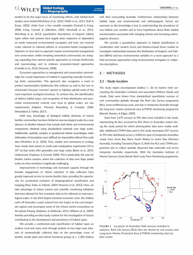
Data from 1,679 surveys at 906 sites were included in the study,

representing all sites surveyed by RLS divers in Australian waters dur-

ing the study period for which photoquadrat data were readily avail-

able. Additional LTMPA data used in this study encompass 857 surveys

at 393 sites distributed across a 4,000 km span of temperate Australian

coasts from Jervis Bay (New South Wales) to Jurien Bay (Western

Australia), including Tasmania (Figure 1). Both the RLS and LTMPA pro-

grammes aim to collect spatially dispersed data nationally and across

temperate Australia, respectively. With the Australian Institute of

Marine Sciences Great Barrier Reef Long-Term Monitoring programme,

FIGURE 1 Locations of Australian field surveys included inanalyses. Reef Life Survey (RLS) sites are shown by red crosses andLong-term Marine Protected Area (LTMPA) monitoring sites byblue circles

2 | CRESSWELL ET AL.

http://www.reeflifesurvey.com

they contribute substantially to Australian State of the Marine Environ-

ment Reporting in the marine realm (Stuart-Smith et al., 2017).

2.2 | Survey methods and data amalgamation

Both the RLS and LTMPA surveys targeted sites characterized by hard

substrata (i.e., rocky or coral reef) in depths < 20 m. The LTMPA sur-

veys quantified macroalgae and sessile invertebrate species in 20 equi-

distant 0.5 m 3 0.5 m quadrats along a 200 m transect line. Each

quadrat was divided into a 7 3 7 grid giving 50 points (including one

corner), under each of which the identity of the species present was

recorded, to the lowest possible taxonomic level, usually to species or

genus. The cover of overstorey/canopy species was recorded first, and

then these were moved aside to expose the understorey for examina-

tion, meaning that > 100% cover was possible (Barrett, Edgar, Buxton,

& Haddon, 2007; Barrett et al., 2009).

The RLS surveys target the same reef types but collect 20 digital

photoquadrats (PQs), each covering c. 0.3 m 3 0.3 m along a 50 m

transect line (see http://reeflifesurvey.com/files/2008/09/rils-reef-

monitoring-procedures.pdf). Further details on the survey methods,

including diver training, data quality assurance and data management,

are covered by Edgar and Stuart-Smith (2009, 2014); Stuart-Smith

et al. (2013). PQs were analysed using a five-point grid superimposed

as a quincunx over each image, under which the uppermost layer of

substrata biota was scored to give an estimate of percentage cover of

38 a priori-defined substratum functional groups. These groups are

listed in Appendix S1 in Supporting Information and are aligned with

the standardized Collaborative and Annotation tools for Marine

Imagery and video (CATAMI) classification scheme used throughout

Australia, as described by Althaus et al. (2015). CATAMI combines

course-level taxonomy and morphology for the consistent classification

of benthic substrates and biota in marine imagery. CATAMI classifica-

tion categories relevant to Australian shallow marine reefs were chosen

for the analyses here.

In order to increase the spatial coverage of data for this study and

combine the RLS PQ data with the higher resolution in situ LTMPA

quadrat data, taxa from the in situ quadrats were mapped to the RLS

substratum biota categories. The percentage cover was then adjusted

to account for scoring of over- and understorey cover in LTMPA quad-

rats and only overstorey in RLS PQs. This was done by an ordered pri-

oritization of the 50 points for canopy formers and then understorey.

Permutational analysis of variance of data from sites at which both RLS

and LTMPA surveys had been conducted was used to test whether the

composition of substratum functional groups recorded from each of

the survey types was comparable for the same sites and regions. The

two survey types were found to give statistically consistent informa-

tion, although marginal, on multivariate functional group structure,

despite differences in survey year and some differences in depths for

the replicate surveys compared from each method (p5 .067; see Sup-

porting Information Appendix S2).

Surveys from either dataset that included patchy areas of non-reef

habitat were either standardized by removing the cover of soft sedi-

ment (if < 50% sand/silt/seagrass) or excluded (if > 50% sand/

seagrass). Both datasets were restricted to surveys conducted between

2006 and 2013 to reduce the influence of potential long-term trends,

while maintaining sufficient spatial coverage. Although transformation

between habitats can occur (Ling, 2008), such phenomena are rela-

tively rare. Consequently, temporal variation over the survey time

period was assumed to be insignificant compared with the continental-

scale spatial variation of interest in the present study.

2.3 | Classification of biogenic reef habitats

Initially, sites within 18 3 18 latitude–longitude grid cells were grouped,

and the mean cover of substratum biota was considered for sites

within these cells to minimize the effect of local-scale variation on the

continental-scale pattern. Hierarchical cluster analysis was used to

group cells that were most similar to each other. Initial clustering (Sup-

porting Information Appendix S3) revealed a clear dichotomy that cor-

responded geographically to a tropical–temperate division (Figure 2).

Tropical and temperate ‘realms’ were demarcated from this cluster

analysis by considering the geography of the two dominant large

groups in the primary analysis, with small and outlying groups merged

with the larger groups according to latitudinal proximity. Principal coor-

dinates analysis (PCaO) confirmed the clear separation of the two dom-

inating tropical/temperate clusters, with 60.6% of the total variation

captured (Supporting Information Appendix S3). Subsequent analyses

could then be conducted separately for these two realms at a site

resolution.

For the tropical analysis, macroalgal categories were binned

because of low cover of macroalgae, whereas in the temperate realm

FIGURE 2 Geographical distribution of seven clusters formed fromhierarchical clustering of 18 3 18 latitude–longitude grid cells. Twoclusters dominated the analysis, one shown in red, populating the lowlatitudes, and the other shown in blue, populating the high latitudes.The small clusters are shown in orange at Shark Bay (WesternAustralia), grey at Geographe Bay (Western Australia), green in UpperSpencer Gulf (South Australia) and Port Phillip Bay (Victoria), pink atEden (New South Wales) and aqua in southern Queensland

CRESSWELL ET AL. | 3

http://reeflifesurvey.com/files/2008/09/rils-reef-monitoring-procedures.pdf

http://reeflifesurvey.com/files/2008/09/rils-reef-monitoring-procedures.pdf

macroalgae dominated the patterns of diversity and abundance, so

individual macroalgal categories were maintained. Stony corals were

grouped together (Supporting Information Appendix S1).

The similarity profiles (Supporting Information Appendix S4) of the

hierarchical cluster analyses of the tropical and temperate realms were

examined to delineate the dominating clusters based on a percentage sim-

ilarity cut-off that was chosen subjectively to yield a workable number of

clusters at a point where small changes in the cut-off point did not drasti-

cally change the number of clusters. The temperate dendrogram was split

at a similarity of 35%, whereas the tropical dendrogramwas split at a simi-

larity of 48%. Clusters with fewer than seven sites were examined individ-

ually and allocated to whichever of the larger clusters groups had greatest

centroid similarity. The resulting clusters of sites were deemed to be dis-

tinct BRHs of Australia’s shallow reef environment.

PCO was used to visualize the separation of the BRHs and confirm

that the resulting groups aligned in ordination space. Vector overlays

based on a Spearman correlation cut-off > 0.4 (Daniel, 1990) were

then used to explore relationships between BRHs and dominant

substrata.

All clustering and coordinate analyses were conducted in PRI-

MERv6 using Bray–Curtis matrices, square-root transformation of data

and group average sorting strategy (Clarke & Gorley, 2006).

2.4 | Environmental and anthropogenic covariates

Nine physical, chemical and anthropogenic variables were used to gain

a better understanding of the spatial relationships between prevalence

and distribution of the BRHs (Supporting Information Appendix S5).

Physical and chemical environmental data were sourced from the Com-

monwealth Scietific and Industrial Research Organization (CSIRO) and

Geoscience Australia (see Huang et al., 2011; Ridgway, Dunn, & Wilkin,

2002). Some potential variables, such as slope and relief bathymetry,

oxygen, salinity and chlorophyll, were not considered because of

known inaccuracy near the coast or inadequate resolution of the avail-

able data. Each site was assigned the environmental characteristics of

the closest node on a 0.58 latitude–longitude grid.

The variables included because of known important roles in struc-

turing marine benthic communities elsewhere (McArthur et al., 2010;

O’Hara & Poore, 2000; Wernberg et al., 2013) comprised sea surface

temperature (mean and SD), spatial predictors (distance to coast and

distance into estuaries for temperate sites given that c. 19% of temper-

ate sites were located < 5 km from or within estuaries) and physical

and chemical variables (wave exposure, cyclone stress, average site

depth, nitrate and phosphate). Nitrate and phosphate were both ini-

tially considered as proxies for nutrient levels but were found to be

highly correlated (r> .65), so only mean nitrate was used in models. A

wave exposure index was calculated from wave height and period

available from the AusWAM 11-year hindcast model (WAMDI Group,

1988) for the temperate sites. These data were not available for tropi-

cal sites. For the tropics, a variable describing cyclone stress was calcu-

lated as the maximal wind speed of any cyclone occurring within

150 km of each site in the previous decade, using data from the NOAA

International Best Track Archive for Climate Stewardship (IBTrACTS)

dataset (https://www.ncdc.noaa.gov/ibtracs/).

Anthropogenic variables were also included to allow the impacts

of human stressors to be considered relative to environmental varia-

bles. A variable describing human population from the Gridded Popula-

tion of the World, Version 4 (GPWv4) population density (2010) was

included as an index, equating to an estimate of people per area (CIE-

SIN, 2014). The marine protection status of each site was also scored

as ‘no take’, ‘restrictions on fishing gear type’ or ‘no restrictions on

fishing’.

2.5 | Covariate analysis

Distance-based linear modelling (DISTLM; Anderson, Gorley, & Clarke,

2008) was used to examine the performance of each environmental vari-

able in explaining the variation in substratum cover between different

sites and between different BRHs. Draughtsman’s plots of the individual

covariates were used to detect extreme bivariate correlations (r� .65)

and to determine whether distributions were skewed. A natural logarithm

transformation was used to correct skewness where necessary. DISTLM

was performed on separate Bray–Curtis similarity matrices for temperate

and tropical realms after data had been square-root transformed. DISTLM

was run using the PERMANOVA1 package in PRIMERv6 (Anderson

et al., 2008), with Akaike information criterion (AIC) and the stepwise

selection procedure with 9,999 permutations. Distance-based redun-

dancy analysis (dbRDA) was then used to test how well environmental

and anthropogenic variables explained variability in site data. Vector over-

lays (r> .4) illustrated the importance and magnitude of each individual

physical variable in explaining variability in the data cloud.

Random forest (RF) models were used to assess which environ-

mental and anthropogenic variables were most closely associated with

each BRH. A RF approach deals with nonlinear relationships and inter-

actions among predictors, as often occur with environmental variables.

Two thousand five hundred trees were generated for each analysis.

Variable importance plots were used to assess the importance of each

predictor variable in the temperate and tropical models and for each

BRH in isolation. Partial dependence plots (Cutler et al., 2007) were

used to provide graphical representation of the marginal effect of the

predictor variables on the probability of each BRH. All random forest

modelling was conducted using the randomForest function in the ran-

domForest package (Liaw & Wiener, 2002) in R (R Core Team, 2014).

3 | RESULTS

3.1 | Biogenic reef habitats

The geographical distribution of clusters showed a biogeographical

dichotomy between tropical and temperate latitudes (Figure 2). Hier-

archical cluster analysis of sites within the temperate realm yielded

four large clusters (each > 28 sites), whereas for the tropical realm five

large clusters were formed (each > 33 sites; Supporting Information

Appendix S4). PCO showed some overlap of clusters, but overall the four

temperate and five tropical clusters were distinguishable on ordination


https://www.ncdc.noaa.gov/ibtracs

(Figure 3). The first two PCO axes for the temperate sites explained

47.2% of the total variation, whereas for the tropical sites it was 45.2%,

indicating that the two-dimensional projections capture nearly half of the

salient patterns in the full data clouds. Clusters were each characterized

by distinct combinations of the mean cover of substratum groups and

were named as separate BRHs accordingly (Table 1).

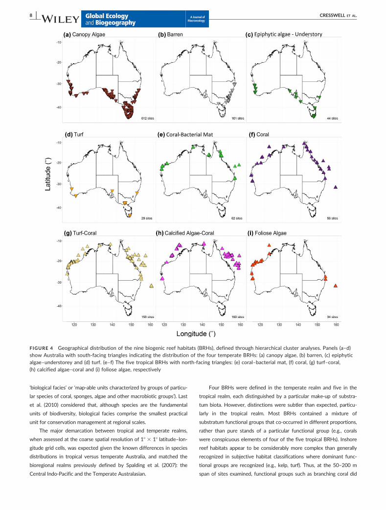
In the temperate realm, the most widespread and prevalent BRH

was canopy algae, occurring in all regions surveyed (Figure 4a). Sites in

the barren BRH were highly concentrated on the New South Wales

coast, together with a few sites on the Victorian and eastern

Tasmanian coasts (Figure 4b). Epiphytic algae–understorey BRH

occurred in a patchy range of locations in southern Australia and

Tasmania (Figure 4c), whereas the turf BRH occurred at six distinct

locations on the Australian coast (Figure 4d).

Tropical BRHs showed a greater mosaic in geographical distribu-

tion compared with the temperate BRHs (Figure 4e–i). In addition, the

tropical BRHs were less clearly defined by particular substratum

groups, with all BRHs except the foliose algae BRH containing a mix of

coral categories (Table 1).

The ‘coral’ BRH occurred in nearly all regions around tropical Aus-

tralia, although it was concentrated on the inshore Queensland coast,

inside the Great Barrier Reef. The ‘turf–coral’ BRH occurred at most

survey locations. ‘Coral–bacterial mat’ occurred in patchy distribution

across the tropical realm. The ‘calcified algae–coral’ BRH occurred at

the most sites and dominated the offshore locations (the Coral Sea and

the North West Shelf). ‘Foliose algae’ was confined to the southern

part of the tropical region in North East Australia, whereas on the west

coast this habitat was evident as far north as the Kimberleys. The turf

BRH did not occur at sites surveyed around most of northern Australia

and the Great Barrier Reef.

3.2 | Environmental and anthropogenic correlates

DISTLM marginal tests for the temperate sites identified all covariates

to have a significant relationship with the multivariate data cloud

derived from the substratum cover of sites. Mean sea surface tempera-

ture (henceforth SST), when considered alone, explained the most vari-

ation (7.6%, p < .001), whereas the human population index explained

6.1% of variation (p < .001). The best model for the temperate realm

included all variables and explained 23.5% of total variation. However,

sequential tests showed mean SST, mean nitrate, estuarine index and

SST standard deviation (henceforth SST SD) cumulatively to explain a

major proportion, 19.1%, of total variation.

The DISTLM marginal tests for the tropical sites showed that SST

SD explained 7.3% (p < .001) of the variation in the data cloud.

Distance to coast and mean SST explained similar proportions: 7.2

(p < .001) and 5.9% (p < .001), respectively. All variables improved the

model fit for the tropical realm, together explaining 23.4% of the varia-

tion in the data cloud. SST SD, mean SST and distance to coast cumula-

tively accounted for 14.9% of variation in the stepwise model

(Supporting Information Appendix S7).

The first and second axes of the temperate dbRDA captured

83.9% of the fitted model but only 19.3% of the total variation of the

substratum biota (Figure 5a). Comparison of the dbRDA ordination to

the corresponding PCO based on temperate data (Figure 3a) indicated

that the DISTLM model has distorted patterns in the data primarily

along the first axis. The vector overlay indicted that the turf BRH

aligned with an increase in estuarine index and a decrease in exposure,

the epiphytic algae–understorey and canopy algae BRHs with high

exposure and low human population indices and the barren BRH with

increasing site depth, nitrate levels, human population and mean SST.

The first two axes of the tropical dbRDA ordination explained

78.0 and 18.3% of the fitted and total variation, respectively (Figure

5b). As for the temperate case, comparison of the dbRDA plot with

the corresponding PCO plot (Figure 3b) showed distortion between

the model representation and the true ordination. The calcified

algae–coral BRH sites were densely clustered and loosely aligned

with increasing distance from the coast, decreasing human popula-

tion index and increasing mean SST and site depth. Both the turf–

coral and the foliose algae groups appeared to align with increased

SST SD and decreasing mean SST. Coral–bacterial mat aligned

loosely with increasing human population indices. The coral BRH

was comparably scattered and with no obvious alignment with varia-

bles in the dbRDA model.

3.3 | Environmental and anthropogenic variables as

predictors for habitat

Tropical and temperate RF models built from the environmental and

anthropogenic variables gave adequate predictions of the BRHs, with

an overall error rate of 15.3% for the temperate model and 24.6% for

the tropical model (percentage of sites classified incorrectly). The RF

variable importance plots (Figure 6) for the temperate and tropical

models showed mean SST to be the most important predictor for both

realms. Human population, wave exposure and mean nitrate were also

ranked highly. In the tropical model, distance to coast, mean nitrate,

SST SD, human population and cyclone stress were of similar

importance.

Depending on the BRH, different variables were more important

for prediction and therefore more highly correlated with a particular

BRH (Figure 7). Partial dependence plots (Supporting Information

Appendix S8) showed the marginal effect of a given variable on the

categorical BRH outcome. Where clear monotonic relationships were

evident between covariates and the partial dependence on a BRH, the

nature of the relationship [positive (1) or negative (2)] is shown on the

variable importance plots (Figure 7).

Nitrate was the most important predictor variable for the canopy

algae BRH, although mean SST and estuarine index, human population

and exposure had similar ranked importance. The probability of classi-

fying a site into the canopy algae BRH increased with higher mean

nitrate and lower mean SSTs and estuarine index according to partial

dependence plots (Figure 7a; Supporting Information Appendix S8).

The barren BRH was best predicted by mean SST, with partial depend-

ence plots indicating that this habitat was more likely with greater mean

SSTs as well as increases in human population index and mean nitrate

(Figure 7b). RF models found that epiphytic algae–understorey BRH was


FIGURE 3 Principal coordinates ordination (PCaO) plot of (a) temperate sites and (b) tropical sites based on the estimated cover ofsubstratum biota. The colours/shapes show, in (a) the four and in (b) the five biogenic reef habitats (BRHs) formed from hierarchical clusteranalysis. Vector overlays show the substratum biota most highly correlated (Spearman correlation coefficient > 0.4) in the data cloud. Thelength of lines in the vector overlay indicate the magnitude of the Spearman correlation coefficient


best predicted by exposure, with mean SST and human population also

highly ranked. Partial plots did not show a clear relationship for exposure;

this BRH was encountered at sites with both low and high exposure val-

ues, with lower frequency between. Exposure and SST mean and SD

were the most important predictors for the turf BRH. As both exposure

and SST SD increased, the probability of turf decreased, whereas a clear

relationship with mean SST was not evident.

The tropical BRHs also showed variability in the most highly

ranked predictor variables (Figure7e–i). Coral–bacterial mat BRH was

most closely associated with the variables SD and mean SST, with par-

tial dependence plots showing that this habitat was unlikely at SST SD

< 1.5 8C, and likelihood increased at high SD values. As mean SST

increased from 22 to 24 8C the likelihood of this habitat increased, but

at higher temperatures the relationship became variable and noisy

(Supporting Information Appendix S8). The coral BRH was most

closely associated with distance to coast and SST SD; however, the

relationship with distance to coast varied in a complex manner. Coral

BRH was more likely at mean SST > 27 8C and at low SDs.

Other than site depth and MPA status, which were relatively low

ranked, variables had similar importance in correctly predicting turf–

coral. Partial plots indicated a higher likelihood of turf–coral with

increasing mean SST and increasing distance to coast. Calcified algae–

coral was best predicted by distance to coast, being most probable far-

ther from shore, at low SST SD and high mean SST. The foliose algae

BRH was most closely associated with human population, distance to

coast and mean SST. The relationship with distance to coast was not

obvious, but partial dependence plots showed higher likelihood at high

human population indices and as mean SST decreased.

4 | DISCUSSION

4.1 | Biogenic reef habitats

On the basis of quantitative analyses, the present study identified nine

distinct broad-scale habitats (BRHs) on shallow reefs surrounding Aus-

tralia. These fit within Level 6 of the 10-level nested hierarchical frame-

work for classifying marine biodiversity of Last et al. (2010; i.e., as

TABLE 1 Nine clusters classified from analyses of sites in the tropical and temperate realms with the mean percentage cover of each of theReef Life Survey substratum biota categories

Temperate Tropical

Biogenic reef habitatCanopyalgae Turf

Epiphytic algae–caulerpa Barren

Foliosealgae

Turf–coral

Calcifiedalgae–coral

Coral–bacterial mat Coral

Sessile taxa categories

Bare rock 2 6 0 23 1 3 10 9 1

Foliose brown algae 5 1 6 3 31 3 0 4 2

Hard branching corals 0 0 0 1 1 2 3 4 9

Branching Acropora 0 0 0 0 0 1 6 11 15

Caulerpa 1 3 15 0 1 1 0 0 0

Crustose coralline algae 4 0 0 30 1 7 21 4 1

Dead coral 0 0 0 1 0 5 1 1 10

Encrusting corals 0 2 0 2 2 8 12 8 6

Filamentous epiphytic algae 1 0 38 0 0 0 0 0 3

Filamentous rock-attached algae 1 14 0 0 0 1 0 0 1

Large brown fucoid kelps 42 5 11 1 10 0 0 1 0

Green calcified algae 0 0 0 0 0 2 12 0 0

Laminarian kelps 24 0 3 3 0 0 0 0 0

Massive corals 0 0 0 0 1 3 5 8 6

Pebbles/coral rubble 1 0 1 3 5 4 6 4 5

Foliose red algae 6 6 13 0 11 2 0 0 0

Bacterial slime on bare rock 1 0 0 9 4 4 1 26 3

Soft corals and gorgonians 0 1 0 0 1 4 5 7 8

Turfing algae 4 52 8 8 18 40 8 3 15

Number of sites in cluster 612 29 44 101 34 158 199 62 56

Note. Percentage cover has been rounded to zero decimal places. Reef Life Survey substratum biota categories with< 5% cover in any biogenic reef habitat(BRH) are not shown here. The full table is available for reference in Appendix S6 in Supporting Information. Bold and italics numbers are those with> 5% cover.


‘biological facies’ or ‘map-able units characterized by groups of particu-

lar species of coral, sponges, algae and other macrobiotic groups’). Last

et al. (2010) considered that, although species are the fundamental

units of biodiversity, biological facies comprise the smallest practical

unit for conservation management at regional scales.

The major demarcation between tropical and temperate realms,

when assessed at the coarse spatial resolution of 18 3 18 latitude–lon-

gitude grid cells, was expected given the known differences in species

distributions in tropical versus temperate Australia, and matched the

bioregional realms previously defined by Spalding et al. (2007): the

Central Indo-Pacific and the Temperate Australasian.

Four BRHs were defined in the temperate realm and five in the

tropical realm, each distinguished by a particular make-up of substra-

tum biota. However, distinctions were subtler than expected, particu-

larly in the tropical realm. Most BRHs contained a mixture of

substratum functional groups that co-occurred in different proportions,

rather than pure stands of a particular functional group (e.g., corals

were conspicuous elements of four of the five tropical BRHs). Inshore

reef habitats appear to be considerably more complex than generally

recognized in subjective habitat classifications where dominant func-

tional groups are recognized (e.g., kelp, turf). Thus, at the 50–200 m

span of sites examined, functional groups such as branching coral did

FIGURE 4 Geographical distribution of the nine biogenic reef habitats (BRHs), defined through hierarchical cluster analyses. Panels (a–d)show Australia with south-facing triangles indicating the distribution of the four temperate BRHs: (a) canopy algae, (b) barren, (c) epiphyticalgae–understorey and (d) turf. (e–f) The five tropical BRHs with north-facing triangles: (e) coral–bacterial mat, (f) coral, (g) turf–coral,(h) calcified algae–coral and (i) foliose algae, respectively


not consistently occur as monotypic entities, but were interspersed

with soft corals, dead coral, turf and a variety of other coral forms

(including massive and encrusting corals).

4.2 | Temperate habitats

The dominant habitat identified in temperate Australia is characterized

by large brown canopy-forming macroalgae (Fucales and Laminariales).

A similar habitat is present in most of the world’s temperate oceans

(Bolton, 2010; Steneck et al., 2002). Globally, altered environmental

regimes, some the direct result of anthropogenic stressors, such as pol-

lution, and others more indirect, arising from flow-on effects of fishing

and climate change, are leading to widespread loss of structurally com-

plex habitats that support diverse communities (Alvarez-Filip, Dulvy,

Gill, Cot�e, & Watkinson, 2009; Connell et al., 2008; Johnson et al.,

2011). Airoldi, Balata, and Beck (2008) describe this change as a ‘flat-

tening’ of the marine environment, with replacement of structurally

complex habitats by more two-dimensional counterparts. Canopy algae

and epiphytic algae–understorey BRHs in the present study represent

architecturally complex habitats that are juxtaposed with the barren

BRH, characterized by bare rock and crustose coralline algae, and turf

BRH, characterized by low-lying mats of turfing algae.

Mean SST was found to be the most important correlate of tropi-

cal and temperate BRHs. Increased SST was positively correlated with

FIGURE 5 Distance-based redundancy analysis (dbRDA) ordinations of (a) temperate sites and (b) tropical sites identifying the greatestvariation between sites based on the cover of substratum functional groups. The vector overlay shows the most strongly correlatedenvironmental variables calculated from the multiple partial correlations (r> .4)


the ‘flat’ habitats (the barren and the turf BRH) and negatively

correlated with the structurally complex canopy algae and epiphytic

algae–understorey BRHs. This is a concern given increasing ocean

temperatures observed and predicted, suggesting that long-term

warming could contribute to the ‘flattening’ of marine habitats. Fur-

thermore, human population was the second most important predic-

tor variable for the temperate RF model and was positively correlated

with barren BRH and negatively correlated with canopy algae and

epiphytic algae–understorey. Thus, our results consistently suggest

that increasing sea temperature and human population growth both

represent key threats to reef habitats and biodiversity via impacts to

structurally complex habitats that support diverse reef-associated

communities. For future studies, examining structural complexity

more quantitatively at the site level would be beneficial; however,

this metric was not available for all sites in the present study

(Alexander, Barrett, Haddon, & Edgar, 2009).

A link between the turf BRH and anthropogenic stressors was evi-

dent in the locations of this habitat. Although human population did

not emerge as a key correlate of this habitat, turf sites were adjacent

to metropolitan coasts (i.e., Hobart, Melbourne, Sydney, Perth), albeit

with additional sites located near Albany (Western Australia) and upper

Spencer Gulf (South Australia), the latter a reverse estuary with

extreme natural disturbance associated with variability in SST and

salinity (Seddon, Connolly, & Edyvane, 2000). The presence of turf

around four of five temperate Australian capital cities implies a link to

anthropogenic pressures, as do prior studies near Adelaide, the fifth

capital city, where displacement of canopy-forming algae by turf mats

has been well documented (Connell et al., 2008; Gorgula & Connell,

2004). Ecological theory suggests that ‘weedy’ plants (fast recruitment,

growth and reproduction), such as turfing algae, are favoured in

environments that are frequently disturbed (such as by human activ-

ities), whereas slower-growing, more structurally complex species, such

as those of the canopy algae BRH, are disadvantaged because of their

life-history strategies (Tilman & Lehman, 2001).

High human population indices were also associated with the bar-

ren BRH, perhaps a consequence of fishing pressure for the key preda-

tors of the urchins responsible for creating this BRH, such as the

southern rock lobster (Jasus edwardsii), blue groper (Achoerodus viridis)

and pink snapper (Pagras auratus) (Ling, Johnson, Frusher, & Ridgway,

2009; Pederson & Johnson, 2006). Canopy algae and barren BRHs had

strong opposing relationships with mean SST and human population,

exemplifying concerns over human-driven shifts from structurally com-

plex to flatter habitats, with the barren BRH representing the lowest-

diversity habitat (Ling, 2008).

4.3 | Tropical habitats

Tropical coral reefs support some of the most diverse marine ecosys-

tems on earth (Green, Bellwood, & Choat, 2009; Sala & Knowlton,

2006), but vary substantially both in the amount of live coral cover and

their structural complexity. Five distinctive tropical BRHs were identi-

fied here, namely coral, coral–bacterial mat, calcified algae–coral, turf–

coral and foliose algae. These were arranged in a complex manner,

both in composition and in spatial distribution.

As for the temperate realm, the major correlate of BRHs in the

tropical realm was mean SST according to both DISTLM and RF results.

Variation in SST was a stronger correlate in the tropical realm than the

temperate, perhaps reflecting low tolerance of corals and other tropical

sessile biotic groups to variation in temperature anomalies. The coral

BRH was characterized by a diverse array of different coral elements

(the genera Pocillopora and Acropora, bleached and dead coral, branch-

ing, massive, encrusting and soft corals) and possessed a strong nega-

tive relationship with SST variability. This, in combination with the

coral BRH occurring frequently at some of the warmest Australian loca-

tions (> 27 8C mean SST), indicates vulnerability to bleaching if the fre-

quency of warm-water events continues to increase.

Turfing algae is a common feature on most coral reefs. This habitat

supports a diverse array of herbivores (Green et al., 2009), which use pro-

duction generated by fast growth and high turnover regardless of low

standing biomass. The turf–coral BRH had c. 40% mean cover of turfing

algae and was associated with high mean SST and large distances off-

shore. It was present at 158 of 509 tropical survey sites in almost all sur-

veyed regions. Although the coral BRH better fits common perceptions

of a diverse coral reef, the degree to which the turf–coral habitat is ‘natu-

ral’ or partially affected by anthropogenic stressors is a key question.

A turfing algae-dominated state has been proposed to occur as an

alternative stable state to coral in tropical ecosystems (Green et al.,

2009; Norstr€om, Nystr€om, Lokrantz, & Folke, 2009). In addition to her-

bivorous fishes, nutrient and light levels are considered important vari-

ables in transitions, with high nutrients and low light levels providing

turfing algae with a competitive advantage over corals, particularly

after disturbances such as cyclones (Hughes et al., 2007). In the present

study, the turf–coral BRH was positively associated with mean nitrate

FIGURE 6 Random forest variable importance plots for (a) thetemperate model and (b) the tropical model. Classification errorsassociated with temperate and tropical models were 15.3 and24.6%, respectively. Plots show the relative importance of the (a)nine and (b) eight covariates in correctly predicting the habitat at agiven site. The percentage change in accuracy for a given predictorvariable is measured by the change in error rate between modelsthat include or do not include that predictor variable (i.e., a largervalue means that variable was more influential in correctlypredicting habitat type). Model output is based on 2,500 trees


concentrations, whereas the coral BRH was negatively associated with

nitrate concentrations, supporting the hypothesis that elevated

nutrients provide a potential competitive advantage for turfs.

Turf mats with heavy loads of cyanobacterial slime are generally

viewed as an undesirable or unhealthy reef state (Green et al., 2009).

In contrast to the coral BRH, the coral–bacterial mat BRH was most

prevalent in areas of high variation in SST. The geographical distribu-

tion of the coral–bacterial mat BRH did not give a clear indication of

oceanic conditions associated with this habitat. Turbidity might play an

important role, as good water quality is a key factor affecting the sur-

vival of coral, whereas cyanobacteria can proliferate as water quality

declines, but was not considered in the present study (Fabricius,

De’ath, McCook, Turak, & Williams, 2005). Coral–bacterial mat

occurred in locations with high amounts of suspended sediment in the

water column attributable to large tidal movement in northwestern

Australia and in the Gulf of Carpentaria (Burford, Alongi, McKinnon, &

Trott, 2008; Somers & Long, 1994).

Foliose algae, with a distribution on the east coast localized near

the Queensland–New South Wales border, and on the west coast

extending northwards along the coast from the Abrolhos Islands, was

associated with high human population, low mean SST relative to other

tropical locations and high variability in SST. The association with

human population index might signify that more frequent anthropo-

genic disturbance is decreasing coral resilience and allowing macroalgae

to expand, although given this habitat occurred most frequently in the

temperate–tropical realm transition, competition between tropical and

temperate species is perhaps a more likely driver.

The calcified algae–coral BRH occurred almost exclusively offshore

(> 200 km), dominating the Coral Sea and North West Shelf. Sites clas-

sified into this group had a high cover of crustose coralline algae, green

FIGURE 7 Results of random forest analyses showing the relative importance of the (a–d) nine and (e–i) eight covariates used to predict thehabitats at a given site. (a–d) The relative importance of the predictors for each temperate biogenic reef habitat (BRH) and (e–i) the relativeimportance of the predictor variables for each of the tropical BRHs. The percentage change in accuracy for a given predictor variable ismeasured by the change in error rate between models that include or do not include that predictor variable (e.g., if mean nitrate is excludedfrom the model, what does that mean for the prediction accuracy for each habitat?). Where clear relationships were evident between covariatesand the partial dependence on a BRH, the nature of the relationship [positive (1) or negative (2)] is shown on the bar plots


calcified algae (Halimeda spp.) and small contributions from a variety of

coral functional groups. The offshore geography of this BRH supports

the findings of Drew (1983) that average biomass of Halimeda spp.

increased with increasing distance from the Great Barrier Reef to the

Coral Sea. Different oceanic conditions at these offshore sites are likely

to be a key driver (Andrews & Clegg, 1989), with high mean SSTs and

low SST variability found as key correlates of this habitat, similar to

those for the coral BRH. Calcified algae probably represents an alterna-

tive to the coral BRH that is maintained by frequent physical disturb-

ance from storm and cyclone activity (calcified algae–coral was

positively correlated with cyclone index).

The DISTLM models captured only a small proportion of total vari-

ation in the tropical models, suggesting that additional unassessed fac-

tors probably play important roles in shaping the broad-scale

distribution of BRHs. For example, light reaching reef benthos in tropi-

cal environments can be affected by turbidity, which was not assessed

in the present study but will contribute to whether a diverse range of

corals or algal turfs prevail. Moreover, much of the variability in habitat

types may occur at local scales < 1 km, whereas this variability could

not be considered in models because of the coarse grain of available

covariate data (typically c. 5 km; Supporting Information Appendix S5).

4.4 | Conclusions

This study examined patterns associated with reef habitat types over a

continental scale using field survey data and includes important infer-

ence about process at the habitat level. Nine BRHs were delineated,

four in the temperate realm and five in the tropical realm, all character-

ized by unique functional sets of algae, sessile invertebrates and corals.

Relationships identified between the objectively defined BRHs and

environmental variables allowed formulation of conceptual models

associated with potential threats to coastal systems (such as increasing

mean SST will lead to decline in the canopy algae and increase in the

barren BRHs). Further research might allow these relationships to be

extended to predict the likelihood of a BRH persisting through time in

any given location, ultimately allowing environmental covariates to be

used as surrogates for cost-effective monitoring. Such an approach

should nevertheless be regarded as an addition rather than alternative

to ongoing benthic monitoring, given that important covariates were

probably overlooked in our study, and unrecognized ecological interac-

tions were probably also present. Improved ecological monitoring can

be achieved through extended application of citizen science, such as

through the Reef Life Survey programme. Further monitoring will allow

conceptual models to be tested and refined, using the current distribu-

tion of habitats as a baseline for assessing future change. Models out-

lined indicate likely influences of local as well as global stressors,

providing guidance to management efforts.

In particular, the association of many BRHs with temperature,

human population and proximity to major cities provides a clear warn-

ing in the context of changing climate and increasing anthropogenic

stress to global marine systems. Particular habitats, including some pre-

viously considered common, such as canopy-forming algae and coral

communities, are threatened.

DATA ACCESSIBILITY

See Supporting Information for more detailed information on analy-

ses, and for the geographical locations of sites within each habitat

type see Appendix S9.

ACKNOWLEDGMENTS

We would like to thank all contributors to the Reef Life Survey and

Temperate Australian Marine Protected Areas monitoring programmes

with special thanks to all persons involved in the analysis of photoqua-

drats. Analyses were facilitated by the Australian Research Council and

the Marine Biodiversity Hub, a collaborative partnership supported

through the Australian Government’s National Environmental Science

Programme. We acknowledge the CSIRO Marine Laboratories as the

source of the CARS2009 environmental data. We gratefully acknowl-

edge Toni Cooper and Just Berkhout for assistance with the RLS data-

set. Thanks also to Simon Wotherspoon, Nicole Hill, Martin Marzloff,

Nick Perkins, Amelia Fowles and Luis Antipa for their interest and

advice regarding the research; to Stuart Kininmonth for contributing

the human population index; to Geoff Hosack for matching the cyclone

data to the study sites; and to George Cresswell and Susan Blackburn

for effective and valuable editing and comments on drafts.

ORCID

Anna K. Cresswell http://orcid.org/0000-0001-6740-9052

Graham J. Edgar http://orcid.org/0000-0003-0833-9001

Rick D. Stuart-Smith http://orcid.org/0000-0002-8874-0083

REFERENCES

Airoldi, L., Balata, D., & Beck, M. W. (2008). The Gray Zone: Relationships

between habitat loss and marine diversity and their applications in con-

servation. Journal of Experimental Marine Biology and Ecology, 366, 8–15.

Alexander, T. J., Barrett, N., Haddon, M., & Edgar, G. (2009). Relationships

between mobile macroinvertebrates and reef structure in a temperate

marine reserve.Marine Ecology Progress Series, 389, 31–44.

Althaus, F., Hill, N., Ferrari, R., Edwards, L., Przeslawski, R., Sch€onberg, C.

H., . . . Colquhoun, J. (2015). A standardised vocabulary for identify-

ing benthic biota and substrata from underwater imagery: the

CATAMI classification scheme. PLoS One, 10, e0141039.

Alvarez-Filip, L., Dulvy, N. K., Gill, J. A., Cot�e, I. M., & Watkinson, A. R.

(2009). Flattening of Caribbean coral reefs: region-wide declines in

architectural complexity. Proceedings of the Royal Society of London B:

Biological Sciences, 276, 3019–3025.

Anderson, M. J., Gorley, R. N., & Clarke, K. R. (2008). PERMANOVA1 for

PRIMER: Guide to software and statistical methods. Plymouth, U.K.:

PRIMER-E.

Andrews, J. C., & Clegg, S. (1989). Coral Sea circulation and transport

deduced from modal information models. Deep Sea Research Part A.

Oceanographic Research Papers, 36, 957–974.

Barrett, N. S., Buxton, C. D., & Edgar, G. J. (2009). Changes in inverte-

brate and macroalgal populations in Tasmanian marine reserves in

the decade following protection. Journal of Experimental Marine Biol-

ogy and Ecology, 370, 104–119.

Barrett, N. S., Edgar, G. J., Buxton, C. D., & Haddon, M. (2007). Changes

in fish assemblages following 10 years of protection in Tasmanian


http://orcid.org/0000-0001-6740-9052

http://orcid.org/0000-0003-0833-9001

http://orcid.org/0000-0002-8874-0083

marine protected areas. Journal of Experimental Marine Biology and

Ecology, 345, 141–157.

Bolton, J. J. (2010). The biogeography of kelps (Laminariales, Phaeophy-

ceae): a global analysis with new insights from recent advances in

molecular phylogenetics. Helgoland Marine Research, 64, 263.

Borer, E. T., Harpole, W. S., Adler, P. B., Lind, E. M., Orrock, J. L., Sea-

bloom, E. W., & Smith, M. D. (2014). Finding generality in ecology: a

model for globally distributed experiments. Methods in Ecology and

Evolution, 5, 65–73.

Burford, M. A., Alongi, D. M., McKinnon, A. D., & Trott, L. A. (2008). Pri-

mary production and nutrients in a tropical macrotidal estuary, Darwin

Harbour, Australia. Estuarine, Coastal and Shelf Science, 79, 440–448.

CIESIN. (2014). Gridded population of the world, version 4 (GPWv4) 2010.

Columbia University, NY: Center for International Earth Science

Information Network.

Clarke, K. R., & Gorley, R. N. (2006). PRIMER v6: User Manual/Tutorial.

PRIMER-E, Plymouth, pp. 192.

Connell, S. D., & Irving, A. D. (2008). Integrating ecology with biogeogra-

phy using landscape characteristics: a case study of subtidal habitat

across continental Australia. Journal of Biogeography, 35, 1608–1621.

Connell, S., Russell, B., Turner, D., Shepherd, A., Kildea, T., Miller, D., . . .

Cheshire, A. (2008). Recovering a lost baseline: missing kelp forests

from a metropolitan coast. Marine Ecology Progress Series, 360, 63–72.

Costello, M. J., Coll, M., Danovaro, R., Halpin, P., Ojaveer, H., & Milosla-

vich, P. (2010). A census of marine biodiversity knowledge, resources,

and future challenges. PLoS One, 5, e12110.

Cracknell, A. P. (1999). Remote sensing techniques in estuaries and coastal

zones an update. International Journal of Remote Sensing, 20, 485–496.

Cutler, D. R., Edwards, T. C., Beard, K. H., Cutler, A., Hess, K. T., Gibson,

J., & Lawler, J. J. (2007). Random forests for classification in ecology.

Ecology, 88, 2783–2792.

Daniel, W. W. (1990). Applied nonparametric statistics (2nd ed.). Boston,

MA: Houghton Mifflin.

Diaz, R. J., Solan, M., & Valente, R. M. (2004). A review of approaches

for classifying benthic habitats and evaluating habitat quality. Journal

of Environmental Management, 73, 165–181.

Douvere, F. (2008). The importance of marine spatial planning in advancing

ecosystem-based sea use management.Marine Policy, 32, 762–771.

Drew, E. (1983). Halimeda biomass, growth rates and sediment genera-

tion on reefs in the central great barrier reef province. Coral Reefs, 2,

101–110.

Edgar, G. J., & Stuart-Smith, R. D. (2009). Ecological effects of marine

protected areas on rocky reef communities: a continental-scale analy-

sis. Marine Ecology Progress Series, 388, 51–62.

Edgar, G. J., & Stuart-Smith, R. D. (2014). Systematic global assessment

of reef fish communities by the Reef Life Survey program. Scientific

Data, 1, 140007.

Fabricius, K., De’ath, G., McCook, L., Turak, E., & Williams, D. M. (2005).

Changes in algal, coral and fish assemblages along water quality gra-

dients on the inshore Great Barrier Reef. Marine Pollution Bulletin, 51,

384–398.

Gorgula, S., & Connell, S. (2004). Expansive covers of turf-forming algae

on human-dominated coast: the relative effects of increasing nutrient

and sediment loads. Marine Biology, 145, 613–619.

Green, A. L., Bellwood, D. R., & Choat, H. (2009). Monitoring functional

groups of herbivorous reef fishes as indicators of coral reef resilience. A

practical guide for coral reef managers in the Asia Pacific Region. Gland,

Switzerland: IUCN. Retrieved from http://cmsdata.iucn.org/down-

loads/resilience_herbivorous_monitoring.pdf

Halpern, B. S., McLeod, K. L., Rosenberg, A. A., & Crowder, L. B. (2008).

Managing for cumulative impacts in ecosystem-based management

through ocean zoning. Ocean and Coastal Management, 51, 203–211.

Huang, S., Stephens, P., & Gittleman, J. (2012). Traits, trees and taxa:

global dimensions of biodiversity in mammals. Proceedings of the

Royal Society of London B: Biological Sciences, 279, 4997–5003.

Huang, Z., Brooke, B. P., Whitta, N., Potter, A., Fuller, M., Dunn, J., & Pitcher, R.

(2011).Australianmarine physical environmental data–Descriptions andmeta-data. Canberra, ACT, Australia: Geoscience Australia. csiro: EP104155.

Hughes, T. P., Rodrigues,M. J., Bellwood, D. R., Ceccarelli, D., Hoegh-Guldberg,

O., McCook, L., . . . Willis, B. (2007). Phase shifts, herbivory, and the resil-

ience of coral reefs to climate change. Current Biology, 17, 360–365.

Irving, A. D., Connell, S. D., & Gillanders, B. M. (2004). Local complexity

in patterns of canopy–benthos associations produces regional pat-

terns across temperate Australasia. Marine Biology, 144, 361–368.

Johnson, C. R., Banks, S. C., Barrett, N. S., Cazassus, F., Dunstan, P. K.,

Edgar, G. J. . . . Taw, (2011). Climate change cascades: Shifts in

oceanography, species’ ranges and subtidal marine community

dynamics in eastern Tasmania. Journal of Experimental Marine Biology

and Ecology, 400, 17–32.

Last, P. R., Lyne, V. D., Williams, A., Davies, C. R., Butler, A. J., & Years-

ley, G. K. (2010). A hierarchical framework for classifying seabed bio-

diversity with application to planning and managing Australia’smarine biological resources. Biological Conservation, 143, 1675–1686.

Liaw, A., & Wiener, M. (2002). Classification and regression by random

forest. R News, 2, 18–22.

Ling, S. D. (2008). Range expansion of a habitat-modifying species leads

to loss of taxonomic diversity: A new and impoverished reef state.

Oecologia, 156, 883–894.

Ling, S. D., Johnson, C. R., Frusher, S. D., & Ridgway, K. R. (2009). Overf-

ishing reduces resilience of kelp beds to climate-driven catastrophic

phase shift. Proceedings of the National Academy of Sciences USA,

106, 22341–22345.

Marzinelli, E. M., Williams, S. B., Babcock, R. C., Barrett, N. S., Johnson,

C. R., Jordan, A., . . . Steinberg, P. D. (2015). Large-scale geographic

variation in distribution and abundance of Australian deep-water kelp

forests. PLoS One, 10, e0118390.

McArthur, M. A., Brooke, B. P., Przeslawski, R., Ryan, D. A., Lucieer, V.

L., Nichol, S., . . . Radke, L. C. (2010). On the use of abiotic surrogates

to describe marine benthic biodiversity. Estuarine, Coastal and Shelf

Science, 88, 21–32.

Mellin, C., Delean, S., Caley, M. J., Edgar, G. J., Meekan, M. G., Pitcher,

C. R., . . . Williams, A. (2011). Effectiveness of biological surrogates

for predicting patterns of marine biodiversity. PLoS One, 6, e20141.

Newman, G., Wiggins, A., Crall, A., Graham, E., Newman, S., & Crowston,

K. (2012). The future of citizen science: Emerging technologies

and shifting paradigms. Frontiers in Ecology and the Environment, 10,

298–304.

Norstr€om, A. V., Nystr€om, M., Lokrantz, J., & Folke, C. (2009). Alternative

states on coral reefs: Beyond coral–macroalgal phase shifts. Marine

Ecology Progress Series, 376, 295–306.

O’Hara, T. D., & Poore, G. C. B. (2000). Patterns of distribution for

southern Australian marine echinoderms and decapods. Journal of

Biogeography, 27, 1321–1335.

Pederson, H. G., & Johnson, C. R. (2006). Predation of the sea urchin

Heliocidaris erythrogramma by rock lobsters (Jasus edwardsii) in

no-take marine reserves. Journal of Experimental Marine Biology and

Ecology, 336, 120–134.

R Core Team. (2014). R: A language and environment for statistical com-

puting. Vienna, Austria: R Foundation for Statistical Computing.


http://cmsdata.iucn.org/downloads/resilience_herbivorous_monitoring.pdf

http://cmsdata.iucn.org/downloads/resilience_herbivorous_monitoring.pdf

Ridgway, K. R., Dunn, J. R., & Wilkin, J. L. (2002). Ocean interpolation by

four-dimensional least squares_application to the waters around Aus-

tralia. Journal of Atmospheric and Oceanic Technology, 19, 1357.

Roff, J. C., & Evans, S. M. J. (2002). Frameworks for marine conservation

— Non-hierarchical approaches and distinctive habitats. Aquatic Con-

servation: Marine and Freshwater Ecosystems, 12, 635–648.

Sala, E., & Knowlton, N. (2006). Global marine biodiversity trends. Annual

Review of Environment and Resources, 31, 93–122.

Seddon, S., Connolly, R. M., & Edyvane, K. S. (2000). Large-scale seagrass

dieback in northern Spencer Gulf, South Australia. Aquatic Botany,

66, 297–310.

Somers, I., & Long, B. (1994). Note on the sediments and hydrology of

the Gulf of Carpentaria, Australia. Marine and Freshwater Research,

45, 283–291.

Spalding, M. D., Fox, H. E., Allen, G. R., Davidson, N., Ferda~na, Z. A.,

Finlayson, M., . . . Robertson, J. (2007). Marine ecoregions of the

world: A bioregionalization of coastal and shelf areas. Bioscience, 57,

573–583.

Steneck, R. S., Graham, M. H., Bourque, B. J., Corbett, D., Erlandson, J.

M., Estes, J. A., & Tegner, M. J. (2002). Kelp forest ecosystems: Bio-

diversity, stability, resilience and future. Environmental Conservation,

29, 436–459.

Stuart-Smith, R. D., Bates, A. E., Lefcheck, J. S., Duffy, J. E., Baker, S. C.,

Thomson, R. J., . . . Edgar, G. J. (2013). Integrating abundance and

functional traits reveals new global hotspots of fish diversity. Nature,

501, 539–542.

Stuart-Smith, R. D., Edgar, G. J., Barrett, N. S., Bates, A. E., Baker, S. C.,

Bax, N. J., . . . Brock, D. J. (2017). Assessing national biodiversity

trends for rocky and coral reefs through the integration of citizen sci-

ence and scientific monitoring programs. BioScience, 67, 134–146.

Tilman, D., & Lehman, C. (2001). Human-caused environmental change:

Impacts on plant diversity and evolution. Proceedings of the National

Academy of Sciences USA, 98, 5433–5440.

Underwood, A. J., Chapman, M. G., & Connell, S. D. (2000). Observations

in ecology: You can’t make progress on processes without under-

standing the patterns. Journal of Experimental Marine Biology and

Ecology, 250, 97–115.

WAMDI Group. (1988). The WAM model—A third generation ocean wave

prediction model. Journal of Physical Oceanography, 18, 1775–1810.

Wernberg, T., Thomsen, M. S., Connell, S. D., Russell, B. D., Waters, J.

M., Zuccarello, G. C., . . . Gurgel, C. F. (2013). The footprint of

continental-scale ocean currents on the biogeography of seaweeds.

PLoS One, 8, e80168.

Williams, A., Bax, N. J., Kloser, R. J., Althaus, F., Barker, B., & Keith, G.

(2009). Australia’s deep-water reserve network: Implications of false

homogeneity for classifying abiotic surrogates of biodiversity. ICES

Journal of Marine Science, 66, 214–224.

Wondolleck, J. M., & Yaffee, S. L. (2017). Marine ecosystem-based man-

agement in practice: Different pathways, common lessons. Island Press,

Washington, pp. 271.

BIOSKETCH

The authors’ research focuses on better understanding of broad-scale

trends in rocky and coral reef biodiversity related to pressures such as

fishing, ocean warming, invasive species and pollution. Analysis of data

collected using standardized methods from the Reef Life Survey pro-

gramme allows the tackling of uniquely broad questions, which encom-

pass not only coral reefs but also rocky reefs from the Antarctic to the

Arctic. The research group’s ultimate goal is to improve monitoring,

reporting, management and protection of marine biodiversity.

SUPPORTING INFORMATION

Additional Supporting Information may be found online in the sup-

porting information tab for this article.

How to cite this article: Cresswell AK, Edgar GJ, Stuart-Smith

RD, Thomson RJ, Barrett NS, Johnson CR. Translating local

benthic community structure to national biogenic reef habitat

types. Global Ecol Biogeogr. 2017;00:1–14. https://doi.org/10.

1111/geb.12620


https://doi.org/10.1111/geb.12620

https://doi.org/10.1111/geb.12620

translating local benthic community structure to national

Documents