transitioning to zero fossil fuel co emissions by 2100 · left, distribution of grid cells with...
TRANSCRIPT

Transitioning to Zero Fossil Fuel CO2 Emissions by 2100
L.D. Danny Harvey Department of Geography
University of Toronto
Presentation at the Aspen Global Change Workshop
Climate Sensitivity on Decadal to Century Timescales:
Implications for Civilization
21 May 2012

Outline of this (and Friday’s) talk:
• Part 1: Assessment of what constitutes ‘catastrophic’ global warming, and what it would take (in terms of reduced CO2 emissions) to have a > 50% chance of avoiding it
• Part 2: Brief overview of my own scenarios directed at (hopefully) avoiding catastrophic global warming • Part 3 (on Friday): Changes in thinking that would be
needed to achieve a scenario that eliminates fossil fuel CO2 emissions by the end of this century
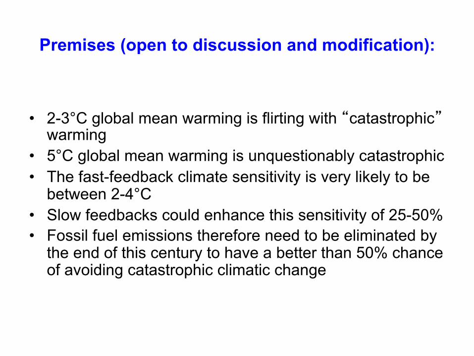
Premises (open to discussion and modification):
• 2-3°C global mean warming is flirting with “catastrophic” warming
• 5°C global mean warming is unquestionably catastrophic • The fast-feedback climate sensitivity is very likely to be
between 2-4°C • Slow feedbacks could enhance this sensitivity of 25-50% • Fossil fuel emissions therefore need to be eliminated by
the end of this century to have a better than 50% chance of avoiding catastrophic climatic change

Some highlights concerning impacts not covered (it appears) by people at
this workshop

Estimated impact of changes in climate trends from 1980-2008 on yields of major crops in major regions. In most regions, the decreases due to climatic trends are superimposed on large increases due improved agricultural technology and techniques. The grey bars
show the most likely changes and the horizontal lines indicate the uncertainty of the estimate (i.e., the true changes are thought to lie anywhere within the changes spanned
by the lines)
Source: Lobell et al. (2011, Science, Vol. 333, 616-620)
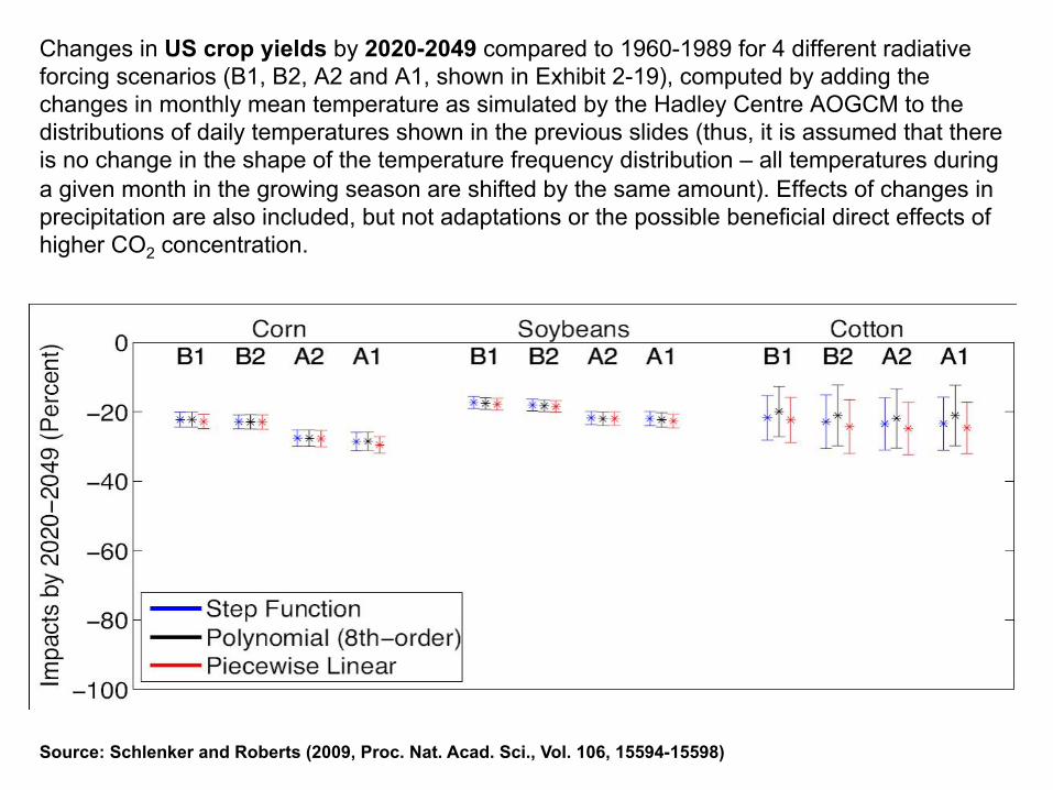
Changes in US crop yields by 2020-2049 compared to 1960-1989 for 4 different radiative forcing scenarios (B1, B2, A2 and A1, shown in Exhibit 2-19), computed by adding the changes in monthly mean temperature as simulated by the Hadley Centre AOGCM to the distributions of daily temperatures shown in the previous slides (thus, it is assumed that there is no change in the shape of the temperature frequency distribution – all temperatures during a given month in the growing season are shifted by the same amount). Effects of changes in precipitation are also included, but not adaptations or the possible beneficial direct effects of higher CO2 concentration.
Source: Schlenker and Roberts (2009, Proc. Nat. Acad. Sci., Vol. 106, 15594-15598)

Same as in previous slide, except that changes by 2070-2099 are shown.
Adaptation and (for soybeans and cotton) the direct physiological effects of higher
atmospheric CO2 would reduce these losses to some extent)
Source: Schlenker and Roberts (2009, Proc. Nat. Acad. Sci., Vol. 106, 15594-15598)

Projected impacts by mid-century of global warming on African staple crops (excluding adaptation).
Source: Schlenker and Lobell (2010, ERL)

Estimate of the impact on crop production (left) and international prices (right) of the 2030 climate compared to the 1990 climate. Worst case: high climatic change, high crop sensitivity, and low CO2 fertilization benefits. Best case: low climatic change and crop sensitivity, maximal CO2 fertilization benefits.
Source: Hertel et al. (2010, Glob. Env. Change 20, 577-585)

Biosphere model projections of fate of the Amazon rainforest by 2090-2100 under the A2 GHG emission scenario. Shown is the extent of
agreement using the changes in climate simulated by 15 different AOGCMs as input to a the LPJ dynamic vegetation model.
Source: Salazar et al. (2007, Geophys. Res. Lett., Vol. 34, L09708)
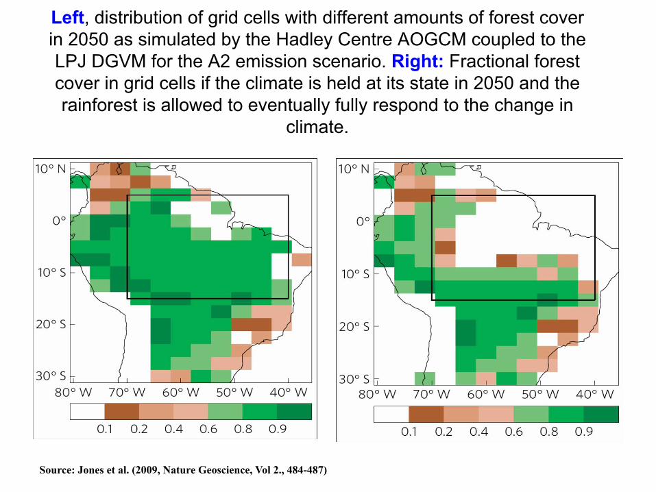
Left, distribution of grid cells with different amounts of forest cover in 2050 as simulated by the Hadley Centre AOGCM coupled to the LPJ DGVM for the A2 emission scenario. Right: Fractional forest cover in grid cells if the climate is held at its state in 2050 and the rainforest is allowed to eventually fully respond to the change in
climate.
Source: Jones et al. (2009, Nature Geoscience, Vol 2., 484-487)

Comparison of the actual Amazonian forest cover (“realized”) at various times in the future in a global warming simulation, and the fractional cover that would eventually remain (“committed”) if the
warming at the time in question were to persist.
Source: Jones et al. (2009, Nature Geoscience, Vol 2., 484-487)

Same data as shown in previous slide, but in terms of realized and committed dieback as a function of the realized temperature change.
Source: Jones et al. (2009, Nature Geoscience, Vol 2., 484-487)

Distribution of maximum wetbulb temperature (Tw) that occurred at any time during the decade 1999-2008. The warmest Tw to have occurred
anywhere is about 30oC.
Source: Sherwood and Huber (2010, Proc. Nat. Acad. Sci., Vol. 107, 9552-9555)

Maximum annual Tw as simulated by an AGCM-ML ocean model after the global mean temperature has warmed by 10oC relative to
1999-2008.
Source: Sherwood and Huber (2010, Proc. Nat. Acad. Sci., Vol. 107, 9552-9555)


Summary of recent estimates of the magnitude of the fast-feedback climate sensitivity
0 1 2 3 4 5 6 7 8 9 10
AML simulations
AOGCM simulations
Historical surface and ocean T trends
Seasonal cycle
Volcanic eruptions
Volcanic eruptions
Recent aerosol decline
Last Glacial Maximum and Late Cretaceous
No aerosols, historical or LGM
Pliocene CO2 vs Temperature*
Simulation of Phanerozoic CO2 variation*
Simulating PETM peak T and C-isotopes*
Climate Sensitivity (K)
?
Williams et al (2008)
Williams et al (2008)
Forest et al (2008)
Knutti et al (2006)
Wigley et al (2005)
Bender et al (2010)
Chylek et al (2007)
Hoffert and Covey (1992)
See text
Pagani et al (2010)
Park and Royer (2011)
Pagani et al (2006)
Methods marked with an asterisk include the effect of changes in vegetation distribution and the full response of ice sheets, but do not include the effect of positive climate carbon cycle feedbacks as the GHG concentrations are taken as a given in computing the climate sensitivity.
Source: Harvey (2012, Fast and Slow Feedbacks in Future Climates, in Future of the World’s Climate)
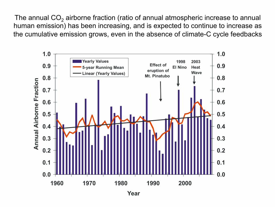
The annual CO2 airborne fraction (ratio of annual atmospheric increase to annual human emission) has been increasing, and is expected to continue to increase as the cumulative emission grows, even in the absence of climate-C cycle feedbacks
0.0
0.1
0.2
0.3
0.4
0.5
0.6
0.7
0.8
0.9
1.0
1960 1970 1980 1990 2000Year
Ann
ualA
irbor
neFr
actio
n
0.0
0.1
0.2
0.3
0.4
0.5
0.6
0.7
0.8
0.9
1.0Yearly Values5-year Running MeanLinear (Yearly Values)
Effect of eruption ofMt. Pinatubo
1998 El Nino
2003HeatWave

In-your-head climate projection, grounded in observations
• BAU cumulative fossil fuel emissions of 2000 GtC (most would say 5000 GtC is possible)
• Average airborne fraction of 0.6 • Peak atmospheric increase is thus 1200 GtC or 600 ppmv • This give a peak concentration of ~ 900 ppmv. • With irreducible increases in other GHGs, this is the equivalent of a
CO2 quadrupling compared to pre-industrial (which was 280 ppmv) • For a climate sensitivity of 1.5-4.5ºC, this gives an expected
equilibrium warming of 3-9ºC • Peak warming could be reduced by 10-20% as the CO2
concentration begins to fall, due to the lag in the full climate response
• HOWEVER – the above does not include all the potential additional CO2 from positive climate-C cycle feedbacks, nor potential feedbacks involving climate and methane
Scenarios that eliminate global fossil fuel emissions before 2100

Original Kaya Identity: Emission = Population x GDP/P x Energy Intensity (MJ/$) x C intensity (kgC/MJ)

Modified Kaya Identity: Emission = Population x Σ(Activity(GDP/P) x Energy/Activity x C intensity )

0
500
1000
1500
2000
2500
3000
2000 2020 2040 2060 2080 2100 2120Year
Popu
latio
n(m
illio
ns)
SASCPASSALAMWEUMENANAMFSUPAOEEU
UNDP Low
Low population scenarios
0
500
1000
1500
2000
2500
3000
3500
2000 2020 2040 2060 2080 2100 2120Year
Popu
latio
n(m
illio
ns) SAS
CPASSALAMWEUMENANAMFSUPAOEEU
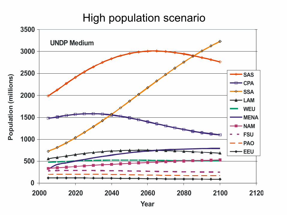
UNDP Medium
High population scenario

0
5000
10000
15000
20000
25000
30000
35000
40000
45000
2000 2020 2040 2060 2080 2100 2120Year
GDP/person(2005$)
NAMWEUPAOEEUCPAFSULAMSASMENASSA
Low
0
10000
20000
30000
40000
50000
2000 2020 2040 2060 2080 2100 2120Year
GDP/person(2005$)
NAMPAOWEUEEUCPAFSULAMSASMENASSA
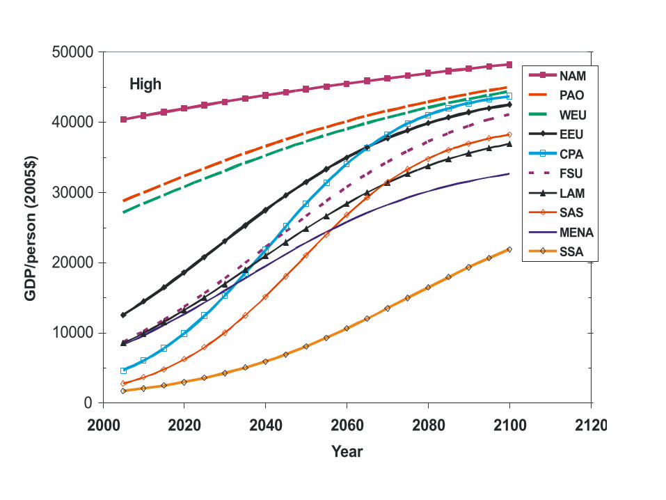
High

Global Results: Population and GDP/P
0
2
4
6
8
10
12
2000 2020 2040 2060 2080 2100Year
Population(billions)
0
8
16
24
32
40
48
AverageGDP/capita(1000s2005$)Population
GDP/capita

0
50
100
150
200
250
300
350
400
2000 2020 2040 2060 2080 2100Year
Wor
ldG
DP
(trill
ions
2005
$)
0
1
2
3
4
Rat
eof
Gro
wth
inG
DP/
P(%
/yr)
World GDP
Rate of growth inworld average GDP/capita
Global Results: GDP and rate of growth in GDP/P

Increasing income is used in a logistic function, calibrated to each socio-economic region in the
model, to drive increasing residential and commercial floor area per capita, increasing total
distance travelled per year per capita, and shifts in the proportion of total travel by light duty vehicles
(LDVs – cars and light trucks) and by air

Illustration of saturation of activity with increasing income, but at different levels in different regions

Energy Intensity Assumptions • Energy performance of new buildings improved by a factor of
~ 4 by 2020 (fast) or 2050 (slow) compared to the performance of recent new buildings
• Retrofits of existing buildings eventually achieve factor of ~ 2-3 reduction in energy use • Complete retrofit or replacement of the entire building stock by
2050 and again by 2100 • Close to maximum currently feasible improvements in
transportation vehicle efficiencies for new vehicles by 2025 or 2035 (this is a factor of 2-3 reduction for a given drive train), and slower improvements thereafter
• Change in modal split (i.e., LDVs to rail) and shift to more energy efficient vehicles in the LDV fraction
• Maximum currently known potential to reduce industrial energy intensities by 2050 + reach 90% recycling of materials by the time the economy reaches a steady state (end of century)

Net Result, Low GDP Scenario:
0
100
200
300
400
500
2000 2020 2040 2060 2080 2100Year
GlobalSecondaryEnergyUse(EJ/yr)
Fuels, slowFuels, slow+shiftFuels, fast+shiftFuels, fast+green+shiftElectricity, slowElectricity, slow+shiftElectricity, fast+shift

Net Result, High GDP Scenario:
0
100
200
300
400
500
2000 2020 2040 2060 2080 2100Year
GlobalSecondaryEnergyUse(EJ/yr)
Fuels, slowFuels, slow+shiftFuels, fast+shiftFuels, fast+green+shiftElectricity, slowElectricity, slow+shiftElectricity, fast+shift

Decomposition of the transition, BAU to zero CO2 emissions in
the transportation sector
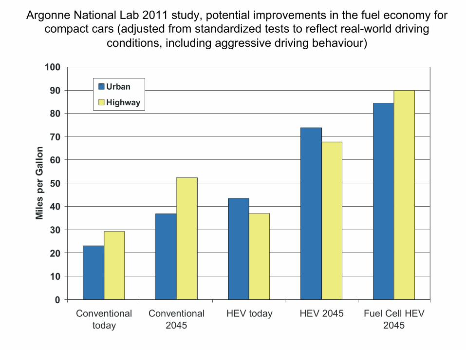
Argonne National Lab 2011 study, potential improvements in the fuel economy for compact cars (adjusted from standardized tests to reflect real-world driving
conditions, including aggressive driving behaviour)
0
10
20
30
40
50
60
70
80
90
100
Conventionaltoday
Conventional2045
HEV today HEV 2045 Fuel Cell HEV2045
MilesperGallon
Urban
Highway

0.0
0.5
1.0
1.5
2.0
2.5
3.0
3.5
4.0
ConventionalToday
HEV 2045 PHEV20 2045 PHEV40 2045 BEV 2045
Ener
gyIn
tens
ity(M
J/km
)
Fuel
Electricity
Argonne National Lab study, fuel and electricity energy intensity for compact cars

0
1
2
3
4
5
6
Compact Mid Size Small SUV Mid Size SUV Pickup truck
EnergyIntensity(MJ/km)
Gasoline ConventionaltodayGasoline HEV Future
H2 fuel cell HEV future
Argonne National Lab study, fuel energy intensity for different vehicle market segments

Technical scenario
• Transition from current to Argonne energy intensities for new vehicles between 2015-2035 or 2015-2045
• Further improvement at 0.5%/yr thereafter • Transition from conventional to PHEV40 drive
train over the same time period • Shift entirely away from pickup trucks and partly
away from SUVs to more efficient vehicles

Resulting global fleet average energy intensity:
0.0
0.2
0.4
0.6
0.8
1.0
2000 2020 2040 2060 2080 2100Year
Rel
ativ
eE
nerg
yU
sepe
rvkm
Slow, fuelsSlow, electricityFast, fuelsFast, electricity

Market shares of the rapidly declining fuel demand
0.0
0.1
0.2
0.3
0.4
0.5
0.6
0.7
0.8
0.9
1.0
2000 2010 2020 2030 2040 2050 2060 2070 2080 2090 2100Year
Mar
ketS
hare Fossil fuels
Biomass in biomass-intensiveBiomass in H2-intensiveH2 in H2-intensive

Global fossil fuel use by LDVs, Low GDP scenario
0
20
40
60
80
100
2005 2015 2025 2035 2045 2055 2065 2075 2085 2095Year
LDV
On-
Site
Foss
ilFu
elU
se(E
J/yr
)Improvement in fuel economyChange in vehicle drive trainChange in vehicle fuelsChange in segment sharesReduction in pkm travelledModal shift away from LDVsIncrease in passenger loadingLess aggressive drivingFinal result

Reductions in global biofuel use by LDVs, Low GDP scenario
0
20
40
60
80
2005 2015 2025 2035 2045 2055 2065 2075 2085 2095Year
LDV
On-
Site
Bio
-Fue
lUse
(EJ/
yr)
Improvement in fuel economyChange in vehicle drive trainChange in segment sharesReduction in pkm travelledModal shift away from LDVsIncrease in passenger loadingLess aggressive drivingExtra final resultFixed fuel share

The Brazilian cerrado, potential land for soybean and sugarcane cultivation and home to > 900 species of birds and 300 species of
mammals, many threatened with extinction
Source: (C) by Luiz Claudio Marigo/naturepl.com

Supply Options, Approach: • Postulate buildup to enough C-free energy sources to
completely displace all fossil fuels by 2100 for each demand scenario
• Consider biomass-intensive and hydrogen intensive supply scenarios
• In the hydrogen-intensive scenario, hydrogen is used in place of biofuels for transportation and industrial uses
• Hydrogen is assumed to be produced by electrolysis of water using C-free electricity sources, and so accounts for about half of the total electricity demand in the
H2-intensive scenarios • Deduce the consequences (in terms of material, energy,
and financial flows, and land area requirements), of the postulated buildup of C-free energy supply
• Evaluate feasibility of the deduced consequences

Electricity Supply Assumptions for the H2-Intensive Scenarios
• Wind – 1500 GW (low GDP) or 3000 GW (high GDP), vs ______239 GW by 2011
• Solar PV – 2000 GW or 4000 GW (vs 40 GW by 2011) • Concentrating solar thermal power – 4500 GW or 9000
___GW (vs 1.2 GW by 2010 but posed for rapid growth) • Biomass – 500 GW or 1000 GW (vs 62 GW in 2010) • Geothermal – 300 GW or 600 GW (vs 11 GW in 2010) • Hydro – increases from 1010 GW in 2010 to 1200 GW in
_______either scenario • No Carbon Capture and Storage • Phase-out of nuclear power (currently at 381 GW)

The total C-free electricity supply in 2100 is thus 11,000 GW for the Low GDP scenario, and 20,800 GW for the High GDP scenario, compared to a total global electricity generating capacity of about 4800 GW in 2010. That is, the C-free electricity capacity required by 2100 is 2-4 times total current electricity capacity

From C. Macilwain (2010, ‘Supergrid’, Nature 468, 624-625)

Figure 2.35a Parabolic Trough Thermal Electricity, Kramer Junction, California

Figure 2.35b Parabolic Trough Thermal Electricity, Kramer Junction, California

Figure 2.35c Close-up of parabolic trough

Molten salt storage tanks at Andasol-1, Spain
Source: Garvin Heath (2009, LCA of Parabolic Trough CSP….), www.nrel.gov/docs/fy09osti/46875.pdf

Figure 12.1c Minimum of CSTP and wind electricity cost (cents/kWh) (excluding transmission cost)
5 6 7 8 10
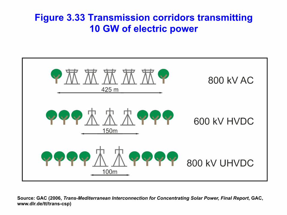
Figure 3.33 Transmission corridors transmitting 10 GW of electric power
Source: GAC (2006, Trans-Mediterranean Interconnection for Concentrating Solar Power, Final Report, GAC, www.dlr.de/tt/trans-csp)
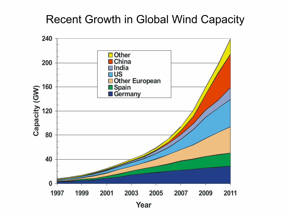
Recent Growth in Global Wind Capacity
0
40
80
120
160
200
240
1997 1999 2001 2003 2005 2007 2009 2011Year
Cap
acity
(GW
)
OtherChinaIndiaUSOther EuropeanSpainGermany

Growth in Annual Additions of Wind Capacity
0
5
10
15
20
25
30
35
40
45
1997 1999 2001 2003 2005 2007 2009 2011
Ann
ualA
dditi
on(G
W/y
r)
OtherChinaIndiaUSOther EuropeanSpainGermany

Recent Growth in Global PV Capacity
0
20
40
60
80
2002 2004 2006 2008 2010Year
Cap
acity
(GW
p-A
C)
Rest of WorldUSAChinaJapanRest of EuropeItalySpainGermany

Growth in Annual Additions of PV Capacity
0
5
10
15
20
25
30
2002 2004 2006 2008 2010Year
Inst
alla
tion
Rat
e(G
Wp-
AC
/yr)
Rest of WorldUSAChinaJapanRest of EuropeItalySpainGermany

Global wind capacity scenarios
0
1000
2000
3000
4000
5000
6000
7000
8000
9000
10000
2000 2010 2020 2030 2040 2050 2060 2070 2080 2090 2100
Year
Cap
acity
(GW
)
HistoricalLow slowLow fastHigh slowHigh fast
Wind Scenarios
Total Global Generating Capacity in 2010

0
100
200
300
400
500
600
2000 2020 2040 2060 2080 2100Year
Rat
eof
Cap
acity
Gro
wth
(GW
/yr)
HistoricalLow slowLow fastHigh slowHigh fast
Wind scenarios

0
500
1000
1500
2000
2500
3000
3500
4000
4500
2000 2020 2040 2060 2080 2100Year
Cap
acity
(GW
)
HistoricalLow slowLow fastHigh slowHigh fast
PV Scenarios

0
20
40
60
80
100
120
140
160
2000 2020 2040 2060 2080 2100Year
Rat
eof
Cap
acity
Gro
wth
(GW
/yr)
HistoricalLow slowLow fastHigh slowHigh fast
PV Scenarios

Areas of bioenergy plantation needed for the biomass-intensive scenarios
0.0
0.5
1.0
1.5
2.0
2000 2020 2040 2060 2080 2100Year
Are
aof
New
Plan
tatio
ns(G
ha)
Series5HSfHFfHSsHFsLSfLFfLSsLFsLFGf
World Cropland Area Today
Scenario

Spatial pattern of the change in NPP over the period 2000-2009 based on the linear trend of satellite-based estimates.
Source: Zhao and Running (2010, Science, Vol. 329, 940-943)

0
2
4
6
8
10
12
2000 2020 2040 2060 2080 2100Year
Foss
ilFu
elC
O2
Em
issi
on(G
tC/y
r)
HSfHFfLSfLFfLFGf
Fast renewable energy rampup
Fossil fuel CO2 emissions

Fossil fuel CO2 emissions
0
2
4
6
8
10
12
2000 2020 2040 2060 2080 2100Year
Fos
silF
uelC
O2
Em
issi
on(G
tC/y
r)
HSs
HFsLSsLFs
Slow renewable energy rampup

Cumulative Fossil Fuel CO2 Emissions
0
200
400
600
800
1000
LSf LFf LFGf HSf HFf LSs LFs HSs HFsScenario
Cum
ulat
ive
Em
issi
on(G
tC)
post-20051800-2005