arX

iv:1

306.

2311

v1 [

astr

o-ph

.SR

] 1

0 Ju

n 20

13Accepted to ApJ: June 7, 2013Preprint typeset using LATEX style emulateapj v. 5/2/11

TRANSIT OBSERVATIONS OF THE HOT JUPITER HD 189733b AT X-RAY WAVELENGTHS

K. Poppenhaeger1,2, J. H. M. M. Schmitt2, S. J. Wolk1

1Harvard-Smithsonian Center for Astrophysics, 60 Garden Street, Cambridge, MA 02138, USA2Hamburger Sternwarte, Gojenbergsweg 112, 21029 Hamburg, Germany

Accepted to ApJ: June 7, 2013

ABSTRACT

We present new X-ray observations obtained with Chandra ACIS-S of the HD 189733 system,consisting of a K-type star orbited by a transiting Hot Jupiter and an M-type stellar companion.We report a detection of the planetary transit in soft X-rays with a significantly larger transit depththan observed in the optical. The X-ray data favor a transit depth of 6-8%, versus a broadbandoptical transit depth of 2.41%. While we are able to exclude several possible stellar origins for thisdeep transit, additional observations will be necessary to fully exclude the possibility that coronalinhomogeneities influence the result. From the available data, we interpret the deep X-ray transit tobe caused by a thin outer planetary atmosphere which is transparent at optical wavelengths, but denseenough to be opaque to X-rays. The X-ray radius appears to be larger than the radius observed atfar-UV wavelengths, most likely due to high temperatures in the outer atmosphere at which hydrogenis mostly ionized. We furthermore detect the stellar companion HD 189733B in X-rays for the firsttime with an X-ray luminosity of logLX = 26.67 erg s−1. We show that the magnetic activity levelof the companion is at odds with the activity level observed for the planet-hosting primary. Thediscrepancy may be caused by tidal interaction between the Hot Jupiter and its host star.Subject headings: planetary systems — stars: activity — stars: coronae— binaries: general — X-rays:

stars — stars: individual (HD 189733)

1. INTRODUCTION

Since the first exoplanet detections almost two decadesago, the research focus of the field has widened frommerely finding exoplanets to characterizing and under-standing their physical properties. Many exoplanetsare found in very close orbits around their host stars– unlike planets in the solar system – and are there-fore subject to strong stellar irradiation. Theoreticalmodels predict that the incident stellar flux can depositenough energy in the planetary atmosphere to lift partsof it out of the planet’s gravitational well, so that theplanetary atmosphere evaporates over time. This evap-oration process is thought to be driven by X-ray andextreme-UV irradiation, and different theoretical modelsemphasize aspects such as Roche lobe effects or hydrody-namic blow-off conditions (Lecavelier des Etangs et al.2004; Lammer et al. 2003; Erkaev et al. 2007). Firstobservational evidence for extended planetary atmo-spheres and possibly evaporation was found for the HotJupiters HD 209458b and HD 189733b, some observa-tions showing temporal variations in the escape rate(Vidal-Madjar et al. 2003; Lecavelier Des Etangs et al.2010; Lecavelier des Etangs et al. 2012). The lower limitof the mass loss, inferred from absorption in H i Lyman-α during transit, was determined to be on the order of& 1010 g s−1, but escape rates may well be several ordersof magnitude larger (Lecavelier des Etangs et al. 2004).Here we investigate the HD 189733 system, located at a

distance of 19.45pc from the Sun. It consists of two stel-lar components and one known extrasolar planet: Theplanet-hosting primary HD 189733A is a main-sequencestar of spectral type K0 and is orbited by a transitingHot Jupiter, HD 189733b, with Mp = 1.138MJup in a

kpoppenhaeger@cfa.harvard.edu

2.22d orbit (see Table 1 for the properties of the star-planet system). There is a nearby M4 dwarf located at11.4′′ angular distance, which was shown to be a physicalcompanion to HD 189733A in a 3200yr orbit based onastrometry, radial velocity and common proper motion(Bakos et al. 2006).HD 189733b is one of the prime targets for plan-

etary atmosphere studies, as it is the closest knowntransiting Hot Jupiter. Different molecules and atomicspecies have been detected in its atmosphere with trans-mission spectroscopy, see for example (Tinetti et al.2007; Redfield et al. 2008). Recent transit obser-vations at UV wavelengths indicate that the tran-sit depth in the H i Lyman-α line might be largerthan in the optical (Lecavelier Des Etangs et al. 2010;Lecavelier des Etangs et al. 2012), possibly indicatingthe presence of extended planetary atmosphere layers be-yond the optical radius. To test this hypothesis, we re-peatedly observed the HD 189733 system in X-rays dur-ing planetary transits.

2. OBSERVATIONS AND DATA ANALYSIS

We observed the HD 189733 system in X-rays duringsix planetary transits with Chandra ACIS-S. One addi-tional X-ray transit observation is available from XMM-Newton EPIC. Another observation was conducted withSwift in 2011; however, this observation has much lowersignal to noise and does not cover the whole transit.The Chandra observations all lasted ≈ 20 ks, the

XMM-Newton pointing has a duration of ≈ 50 ks, andall data sets are approximately centered on the transit(see Table 2 for details of the observations). The orbitalphase coverage is therefore highest for phases near thetransit, with the transit lasting from 0.984−1.016 (first tofourth contact); the phase coverage quickly decreases for

2

stellar parameters:

spectral type K0Vmass (M⊙) 0.8radius (R⊙) 0.788distance to system (pc) 19.3

planetary parameters:

mass × sin i (MJup) 1.138optical radius (RJup) 1.138semimajor axis (AU) 0.03142orbital period (d) 2.21857312mid-transit time (BJD) 2453988.80261orbital inclination 85.51◦

TABLE 1Properties of the HD 189733 Ab system, as given in theExtrasolar Planet Encyclopedia (www.exoplanet.eu).

Instrument ObsID start time duration(ks)

XMM-Newton EPIC 0506070201 2007-04-17 14:06:57 54.5Chandra ACIS-S 12340 2011-07-05 11:56:51 19.2Chandra ACIS-S 12341 2011-07-21 00:23:17 19.8Chandra ACIS-S 12342 2011-07-23 06:18:51 19.8Chandra ACIS-S 12343 2011-07-12 03:26:19 19.8Chandra ACIS-S 12344 2011-07-16 13:45:59 18.0Chandra ACIS-S 12345 2011-07-18 19:08:58 19.8

TABLE 2X-ray observation details for the HD 189733 system.

smaller or larger phases until coverage is only provided bythe single XMM-Newton observation (see Fig. 2). Chan-dra uses a dithering mode; this does not produce signalchanges in the observations 1, 2, 3, 4, and 6. In observa-tion 5, the source was dithered near a bad pixel column,resulting in the loss of a few photons every 1000 s. Thetransit lasts ca. 6500 s and the fraction of missing pho-tons is slightly larger out of transit than during transit,so that no spurious transit signal or limb effects can beproduced by this.

2.1. Spatially resolved X-ray images of the HD 189733system

All previous obervations of the HD 189733 systemhad been performed with XMM-Newton; due to therather broad PSF of the prime instrument PN (ca. 12.5′′

FWHM), the secondary HD 189733B was not properlyresolved in those observations. Our Chandra observa-tions with a PSF of ca. 0.5′′ (FWHM) fully resolve thestellar components for the first time; a soft X-ray imageextracted from one single Chandra exposure with 20 ksduration is shown in Fig. 1. The primary HD 189733Ais shown in the center, the secondary HD 189733B tothe lower right at an angular distance of 11.4′′ to theprimary, and a background source at the bottom of theimage at an angular distance of 11.7′′. The planetary or-bit of HD 189733b is not resolved in these observations:if observed at quadrature, its angular distance to the hoststar would be ca. 1.6mas.

2.2. Individual light curves

To inspect the individual X-ray light curves ofHD 189733A, HD 189733B, and the background source,we extracted X-ray photons from an extraction region

Fig. 1.— X-ray image of the planet-hosting star HD 189733A(upper left object), its companion star HD 189733B (right object)and a background object (lower object). The image is extractedfrom a single Chandra exposure with an integration time of 20 ksin the 0.1-5 keV energy band. The companion HD 189733B is de-tected for the first time in X-rays with these observations.

centered on each source with 2.5′′ radius for the Chan-dra observations. We restricted the energy range to0.1-2.0keV for HD 189733A and HD 189733B, becausepractically no stellar flux at higher energies was present;we used an energy band of 0.1-10.0 keV for the back-ground source. For the archival XMM-Newton observa-tion, we chose an extraction radius 10′′ to collect mostof the source photons from HD 189733A while avoid-ing strong contamination from the other two sources.XMM-Newton EPIC/PN provides sensitivity down to0.2 keV, so we restricted the energy range to 0.2-2.0 keV.In all Chandra observations the background signal wasneglibigly low and constant (0.05% of the source countrate). For XMM-Newton, the background signal is weakand only slightly variable during times that are inter-esting for the transit analysis (ca. 2% of the sourcecount rate); however, in the beginning of the observationthe background is stronger, and we therefore followedthe standard procedure and extracted photons from alarge source-free area, scaled down this background sig-nal to the source extraction area and subtracted thebackground signal from the XMM-Newton source lightcurve.For the light curves, we chose time bin sizes suited to

obtain reasonable error bars; specifically, the chosen binsize is 200 s for HD 189733A, 1000 s for HD 189733B, and500 s for the background source.

2.3. Phase-folded light curve

To test if a transit signal can be detected in the X-ray data, we also constructed a phase-folded, added-upX-ray light curve. We corrected all X-ray photon arrivaltimes with respect to the solar system barycenter, usingthe ciao4.2 task axbary for the Chandra events and theSASv11.0 task barycen for the XMM-Newton events. Or-bital phases were calculated using the mid-transit timeand orbital period given in the Extrasolar Planet Ency-clopaedia and are listed in Table 1. We first extractedlight curves from the individual observations with a very

3

Fig. 2.— Cumulative phase coverage of the available X-ray datafor HD 189733A near the planetary transit. The added exposuresare normalized to unity; at this maximum value, a given phase iscovered by seven individual X-ray observations. The duration ofthe optical transit (first to fourth contact) is depicted by dashedvertical lines.

small time binning (10 s). We normalized the light curvesto an out-of-transit level of unity, chose the desired phasesegments (0.005, corresponding to roughly 16 minutes),and added up the individual observations to form thebinned phase-folded lightcurve, giving the same weightto each individual light curve. These 0.005 phase binscontain ≈ 500 X-ray photons each. The error bars ofthe individual light curves are dominated by Poissoniannoise, which is close to Gaussian noise given the num-ber of X-ray counts per 0.005 phase bin; these errorswere propagated to the added-up light curve. Because ofthe intrinsic variability of the stellar corona it is impor-tant to average over the individual transit observations.We therefore restrict our analysis to orbital phases atwhich at least six of the seven observations provide sig-nal. Specifically, this is given at orbital phases between0.9479 to 1.0470.

2.4. Spectra

We extracted CCD spectra of all three sources from theChandra ACIS-S exposures. We used a minimum binningof 15 counts per energy bin; for the secondary, we usedsmaller bins with ≥ 5 counts per bin because of the lowcount rate. We fitted the resulting six spectra of eachsource simultaneously in Xpsec v12.0, therefore ignoringspectral changes inbetween the individual observationsand focusing on the overall spectral properties of eachobject. We fit the spectra with thermal plasma modelsfor HD 189733A and HD 189733B; since we do not knowthe exact nature of the third source a priori, we test athermal plasma model and a power law model for fit-ting those spectra. We use elemental abundances fromGrevesse & Sauval (1998) for all spectral fits.A detailed analysis of HD 189773A’s spectrum ob-

served with XMM-Newton (out of transit) was performedbefore; see Pillitteri et al. (2010), Pillitteri et al. (2011).

3. RESULTS

3.1. HD 189733A: Individual light curves and spectra

Fig. 3.— Individual X-ray light curves of HD 189733A whichcover the planetary transit, with a time binning of 200 s and 1σPoissonian error bars. All light curves are extracted from an energyrange of 0.2-2 keV.

The individual X-ray light curves of HD 189733A areshown in Fig. 3. The mean count rate is at ≈ 0.07 cts s−1

for Chandra’s ACIS-S, and at ≈ 0.15 cts s−1 for XMM-Newton’s EPIC.An inspection of these light curves shows their intrinsic

variability to be quite small for an active star with max-imum count rate variations being less than a factor oftwo. Such small changes are often found to be the baselevel of variability in cool stars, and are referred to as”quasi-quienscence” (Robrade et al. 2010). Larger flarescan be superimposed on this type of variability, but thisis not the case for our observations of HD 189733A.However, small flare-shaped variations are present, for

example in the second Chandra light curve at orbitalphase 1.01. For the X-ray flares of HD 189733 whichhave been detected with XMM-Newton at other orbitalphases, Pillitteri et al. (2010, 2011) show that changes inthe hardness ratio do not always accompany the flares, sothat we focus on the light curves as a primary flare indi-cator for our observations. We show the individual lightcurves split up into a hard and soft band (0.2-0.6 keV,0.6-2 keV) together with the total band in Fig. 4, usinga bin size of 300 s to have reasonable photon statisticsfor the individual bands. We test for correlated intensitychanges in both bands in detail in section 3.5.3, find-ing that the second Chandra observation and the XMM-Newton observation likely contain small stellar flares.The source spectra of HD 189733A, extracted from the

4

Fig. 4.— The individual X-ray light curves of HD 189733A indifferent energy bands (light grey: 0.2-0.6 keV, grey: 0.6-2.0 keV,black: full energy band), with a time binning of 300 s.

object HD 189733A HD 189733BT1 (keV) 0.25± 0.01 0.32± 0.02norm1 (1.81± 0.1)× 10−4 (5.1± 0.5)× 10−6

EM1 (1050 cm−3) 7.7± 0.4 0.22± 0.02T2 (keV) 0.62± 0.03 1.25± 0.5norm2 (6.6± 0.5)× 10−5 (1.7± 0.5)× 10−6

EM2 (1050 cm−3) 2.8± 0.2 0.07± 0.02O 0.31± 0.02 (fixed at solar)Ne 0.25± 0.13 (fixed at solar)Fe 0.64± 0.05 (fixed at solar)

χ2

red(d.o.f.) 1.43 (279) 1.12 (64)

FX (0.25-2 keV) 2.63× 10−13 1.1× 10−14

logLX (0.25-2 keV) 28.1 26.67

TABLE 3Thermal plasma models for the X-ray emission of the

primary and secondary star. Flux is in units oferg s−1 cm−2, luminosity in units of erg s−1. The emissionmeasure is derived from Xspec’s fitted normalization bymultiplying it with 4π d2 × 1014, with d being the distance

to the two stars.

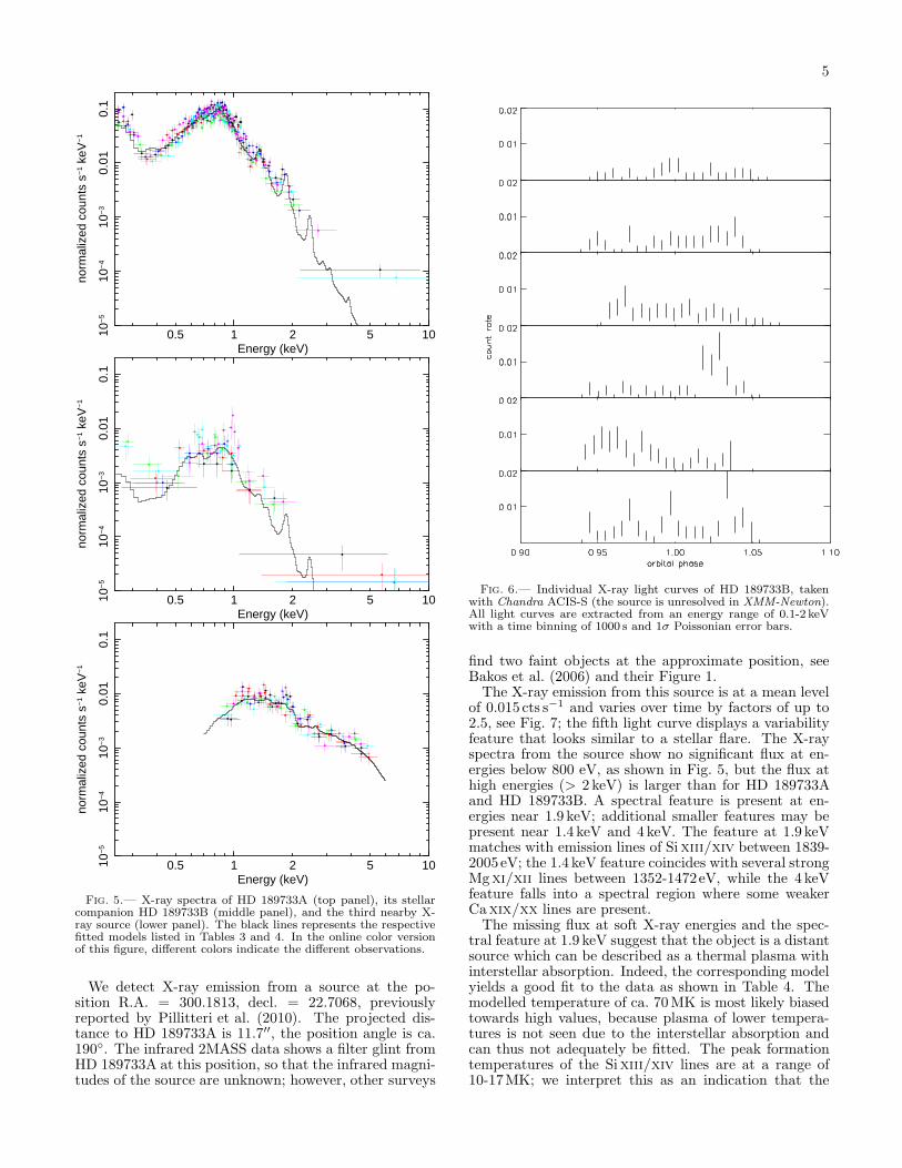
six Chandra ACIS-S pointings, are shown in Fig. 5, toppanel. The dominant part of the emission is at ener-gies below 2 keV, and all six observations display verysimilar energetic distributions and intensities. We fit-ted the spectra simultaneously with a thermal plasmamodel; two temperature components and variable abun-dances for the most prominent elements at soft X-rayenergies (oxygen, neon, and iron) are necessary for a de-

cent fit quality. We find a mean coronal temperature ofca. 4.5MK, with a dominant temperature component atca. 3MK (see Table 3). Our spectral fit yields an X-rayflux of 2.63×10−13 erg cm−2 s−1 in the 0.25-2 keV energyband, corresponding to an X-ray luminosity of LX =1.1× 1028 erg s−1. We calculate HD 189733A’s bolomet-ric luminosity, using bolometric corrections from Flower(1996), to be Lbol = 0.35 × Lbol,⊙ = 1.3 × 1033 erg s−1.The ratio of X-ray to bolometric luminosity is thereforeRX = LX/Lbol = 10−5, characterizing HD 189733A asa moderately active star; the Sun, for comparison, emitsvarying X-ray flux fractions of about 10−6− 10−7 duringits activity cycle.The coronal abundances show a FIP-bias, meaning

that the abundances of elements with a high firstionization potential (oxygen and neon) are lower thanthe abundances of low-FIP elements (iron); all abun-dances are given relative to solar photospheric values(Grevesse & Sauval 1998). This effect is observed incoronae of stars with low to moderate activity, whilehigh-activity stars show an inverse FIP-effect. Recently,a possible correlation of FIP-bias with spectral typehas been found for inactive and moderately active stars(Wood & Linsky 2010). Our measured abundances forHD 189733A fit into this pattern: The average logarith-mic abundance of neon and oxygen relative to iron is−0.41 here, and Wood & Linsky (2010) predict similarvalues around −0.35 for stars of spectral type K0.

3.2. HD 189733B

We detect the stellar companion HD 189733B in X-rays for the first time. It displays a mean count rateof ≈ 3 cts ks−1, with considerable variability by up toa factor of 5. The fourth light curve (Fig. 6) displaysa prominent flare-like variation which lasts for ca. 6 ks.Variability on shorter time scales is also implied by theother light curves, but individual small flares cannot becharacterized properly due to the low count rate.The spectra of HD 189733B are well described by a

thermal plasma with two temperature components, witha dominant temperature contribution at ca. 3.5MK(see Table 3). The collected spectral counts are notsufficient to constrain elemental abundances in thecorona, and therefore we fixed the abundances at so-lar values. The spectral fit yields an X-ray luminos-ity of logLX = 26.67 erg s−1 in an energy range of0.25 − 2 keV. This is compatible with the upper limitof logLX ≤ 27 erg s−1 derived from XMM-Newton ob-servations by Pillitteri et al. (2010). In the context oflate-type stars in the solar neighborhood, HD 189733Bis slightly less X-ray luminous than the median valueof logLX = 26.86 erg s−1 found for early M dwarfs(Schmitt et al. 1995). To calculate the bolometric lu-minosity of HD 189733B, we use the relations fromWorthey & Lee (2011): the measured H − K color of0.222 and a spectral type between M3.5V and M5V(Bakos et al. 2006) translates to a bolomeric correctionof BCV = −2.05 to a V magnitude of 14.02, yieldingLbol = 1.8× 1031 erg s−1. The X-ray fraction of the totalbolometric flux is therefore RX = LX/Lbol = 2.5×10−5,marking HD 189733B as a moderately active M star.

3.3. The background source

5

1 100.5 2 510−

510

−4

10−

30.

010.

1

norm

aliz

ed c

ount

s s−

1 ke

V−

1

Energy (keV)

1 100.5 2 510−

510

−4

10−

30.

010.

1

norm

aliz

ed c

ount

s s−

1 ke

V−

1

Energy (keV)

1 100.5 2 510−

510

−4

10−

30.

010.

1

norm

aliz

ed c

ount

s s−

1 ke

V−

1

Energy (keV)

Fig. 5.— X-ray spectra of HD 189733A (top panel), its stellarcompanion HD 189733B (middle panel), and the third nearby X-ray source (lower panel). The black lines represents the respectivefitted models listed in Tables 3 and 4. In the online color versionof this figure, different colors indicate the different observations.

We detect X-ray emission from a source at the po-sition R.A. = 300.1813, decl. = 22.7068, previouslyreported by Pillitteri et al. (2010). The projected dis-tance to HD 189733A is 11.7′′, the position angle is ca.190◦. The infrared 2MASS data shows a filter glint fromHD 189733A at this position, so that the infrared magni-tudes of the source are unknown; however, other surveys

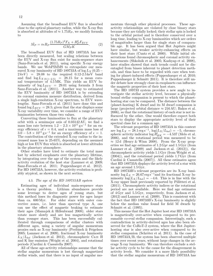
Fig. 6.— Individual X-ray light curves of HD 189733B, takenwith Chandra ACIS-S (the source is unresolved in XMM-Newton).All light curves are extracted from an energy range of 0.1-2 keVwith a time binning of 1000 s and 1σ Poissonian error bars.

find two faint objects at the approximate position, seeBakos et al. (2006) and their Figure 1.The X-ray emission from this source is at a mean level

of 0.015 cts s−1 and varies over time by factors of up to2.5, see Fig. 7; the fifth light curve displays a variabilityfeature that looks similar to a stellar flare. The X-rayspectra from the source show no significant flux at en-ergies below 800 eV, as shown in Fig. 5, but the flux athigh energies (> 2 keV) is larger than for HD 189733Aand HD 189733B. A spectral feature is present at en-ergies near 1.9 keV; additional smaller features may bepresent near 1.4 keV and 4 keV. The feature at 1.9 keVmatches with emission lines of Sixiii/xiv between 1839-2005eV; the 1.4 keV feature coincides with several strongMgxi/xii lines between 1352-1472eV, while the 4 keVfeature falls into a spectral region where some weakerCaxix/xx lines are present.The missing flux at soft X-ray energies and the spec-

tral feature at 1.9 keV suggest that the object is a distantsource which can be described as a thermal plasma withinterstellar absorption. Indeed, the corresponding modelyields a good fit to the data as shown in Table 4. Themodelled temperature of ca. 70MK is most likely biasedtowards high values, because plasma of lower tempera-tures is not seen due to the interstellar absorption andcan thus not adequately be fitted. The peak formationtemperatures of the Sixiii/xiv lines are at a range of10-17MK; we interpret this as an indication that the

6

Fig. 7.— Individual X-ray light curves of the third source, takenwith Chandra ACIS-S. All light curves are extracted from an energyrange of 0.1-10 keV with a time binning of 500 s and 1σ Poissonianerror bars.

model parameters abs. thermal plasma abs. power law

nH (4.5± 0.6)× 1021 (5.8 ± 0.7) × 1021

T (keV) 6.0± 0.9 -photon index - 1.9± 0.1norm (1.1± 0.06) × 10−4 (3.9 ± 0.5) × 10−5

χ2

red(d.o.f.) 1.12 (99) 1.11 (99)

FX (0.25-10 keV) 1.44× 10−13 1.47 × 10−13

logLabsX (0.8-10 keV) 31.2 31.2

logLunabsX

31.4 31.4

TABLE 4Spectral fits for the X-ray emission of the third source.An absorbed thermal plasma model and an absorbed powerlaw both yield good fits. The absorbed and unabsorbed

X-ray luminosities are calculated using a distanceestimate of 1000 pc.

average plasma temperature is significantly lower than70MK. We assume from the fitted hydrogen absorptionwith a column density of nH = 4.5× 1021 cm−2 that thesource is located at a distance of roughly 1000pc fromthe Sun, consistent with Pillitteri et al. (2010). Withthis distance, the measured flux converts to an intrinsic(unabsorbed) X-ray luminosity of logLX = 31.4 erg s−1.So what is the nature of this source? Its position in

galactic coordinates is l = 60.9623, b = −03.9227, mean-ing that it lies in the galactic plane in a viewing direction60◦ off the galactic center, possibly on the Orion-Cygnusarm. Together with the rough distance estimate from

hydrogen absorption, the emission feature in the spec-tra and the flare-shaped variation in the light curves,we consider it likely that the source is an RS CVn orAlgol system. Its X-ray luminosity is at the high end,but still in the range of observed values for such systems(Walter et al. 1980; White & Marshall 1983).For completeness, we note that a model with an ab-

sorbed power law formally yields an equally good fit, butdoes not explain the observed feature at 1.9 keV. Adopt-ing the power law model, we find similar values for hy-drogen absorption and X-ray luminosity (see Table 4).

3.4. The phase-folded X-ray light curve of HD 189733A

We now turn to a detailed analysis of the phase-foldedand added up X-ray transit light curve of the Hot JupiterHD 189733Ab.

3.5. Testing for autocorrelation and red noise

As a first step, we test if the scatter in the observedindividual and added-up light curves is sufficiently welldescribed by white noise. If the sequence of measuredcount rates is not randomly distributed on time scalesshorter than the transit, but is correlated in some way,this would require a more detailed treatment of the noiselevel. We have therefore tested for autocorrelation inthe individual light curves, as well as for deviations fromwhite noise in the added-up light curve, both with neg-ative results. This analysis is presented in detail in theAppendix.

3.5.1. A transit detection in X-rays

As a second step, we investigate if the transit is de-tected in the soft X-ray light curves by testing if the nullhypothesis of a constant X-ray count rate in and out oftransit can be rejected. To use as few assumptions aspossible, we use only orbital phases during which all ofthe observations provide data for this; specifically, we useorbital phases between 0.9560 and 1.0345. This makes itpossible to compare the raw (i.e. unnormalized) numberof detected soft X-ray photons in and out of transit. Forthe XMM-Newton observations we use the net numberof source photons, i.e. the source signal corrected for thelow-level background signal. We define orbital phases be-tween second and third contact as ”in transit” and phasesbefore first or after fourth contact as ”out of transit”. Wethen add up the detected X-ray photons of all seven lightcurves in and out of transit, divide by the duration of thein and out of transit times, and compute the χ2 goodnessof fit to a constant model with the overall average photonrate. We list the in and out of transit count rates, the χ2

value, and the confidence at which the null hypothesisof a constant count rate can be rejected in Table 5. Wefind that for all seven datasets combined, the null hy-pothesis can be rejected at 98.00% confidence. For othercombinations of five or six datasets (which are motivatedbelow in section 3.5.3), we find confidence levels between98.39% and 99.80%. Having shown that we have indeeddetected the transit of the exoplanet in X-rays with highconfidence, we proceed by deriving the transit depth.

3.5.2. Deriving the transit depth

We have one observation that starts relatively late(Chandra light curve 3) and one that ends early (Chan-dra light curve 5). To increase our accuracy for a transit

7

(a) all 7 data (b) 6 data sets, (c) 6 data sets, (d) 5 non-flaringsets excluding flaring excluding flaring data sets

Chandra observation XMM-Newton observation

raw count rate in transit (cts s−1) 0.4696± 0.0106 0.4122 ± 0.0099 0.3249 ± 0.0088 0.2675± 0.0080raw count rate out of transit (cts s−1) 0.4996± 0.0075 0.4467 ± 0.0071 0.3508 ± 0.0063 0.2979± 0.0058χ2 of constant model 5.41 8.08 5.79 9.58constant model rejected at confidence 98.00% 99.55% 98.39% 99.80%

TABLE 5Added-up raw count rate (i.e. without pre-normalization) in and out of transit, for the four combinations of data sets

discussed in section 3.5.3, together with the confidence level at which a constant model is rejected.

depth measurement, we therefore pre-normalized the in-dividual transit light curves to an out-of-transit level ofunity and use a larger orbital phase range between 0.9479and 1.0470, as described in section 2.3.We used three different statistical methods to deter-

mine the depth of the X-ray transit in the phase-foldedlight curve; they are explained in the following and theirresults are listed in Table 6.(1) The mean normalized X-ray count rates in and out

of transit were compared directly. We have defined datafrom orbital phases between second and third contactas ”in transit” and data from phases before first or afterfourth contact as ”out of transit”. Since the total numberof X-ray photons is large, differences between Poissonianand Gaussian errors are negligible, and we have usedGaussian error propagation to determine the error onthe transit depth as σdepth =

√

σ2in + σ2

out.(2) We have fitted the data to an analytical tran-

sit model as used for optical, limb-darkened transits(Mandel & Agol 2002). This will not be entirely correct,because coronae are limb-brightened, not limb-darkenedlike photospheres (see method 3). However, we give thefitting results to photospheric transit profiles for com-pleteness. Specifically, we fixed the planetary orbital pe-riod, semimajor axis, mid-transit time, and inclinationto the values given in the Extrasolar Planets Encyclo-pedia, used a quadratic limb darkening law with coeffi-cients u1 = 0.32 and u2 = 0.27 as used for the opticallight curve (Winn et al. 2007) depicted in Fig. 8(a), andperformed a Markov-Chain Monte Carlo fit with the ra-

tio of the planetary and stellar radius RX−rayP /R∗ as a

free parameter.(3) The stellar corona is optically thin, so that it

shows limb brightening instead of the limb darkening ob-served in the photosphere. We have taken this into ac-count by fitting the data with a limb-brightened model(Schlawin et al. 2010) under the assumption that thecorona is not significantly extended beyond the photo-spheric radius. This is a valid assumption: It is knownthat individual flaring loops in active stars may extendquite far over the photospheric radius, but the averagecorona of active stars apparently is not much extended.This was directly observed in the case of the binaryα CrB, where the X-ray dark A star eclipses the active,X-ray bright G star without significant timing differencesfrom the optical transit profile (Kuerster & Schmitt1996). We again fixed the planetary orbital period, semi-major axis, mid-transit time, and inclination, and fittedthe ratio of the planetary and stellar radius. The result-ing transit profile is shown as a dashed line in Fig. 8(a).

3.5.3. Light curve selection

The stellar corona is much less homogeneous than thestellar photosphere. X-ray emitting coronal loops aretemporally variable, and solar observations show that itscorona often displays several large, X-ray bright patches,while other parts are dimmer in X-rays. This is why itis unlikely to identify a planetary transit signal in a sin-gle X-ray light curve, even if the signal to noise is veryhigh: It is possible that, given a specific configurationof X-ray bright patches of the corona, the planet hap-pens to transit a mostly X-ray dim part. On the otherhand, the planet may occult a large X-ray bright patchin a different coronal configuration, causing an untypi-cally deep transit signal. One therefore needs to averageover as many transits as possible to determine the transitdepth with respect to the typical, average X-ray surfacebrightness of a corona.To show the importance of the coronal averaging, we

determined the observed transit depths (derived from thedirect count rate comparison) for different combinationsof the X-ray light curves. With a total of seven transitlight curves, there is one combination which includes alllight curves, and seven combinations which include six ofthe light curves. Given the relatively low overall numberof X-ray photons, we do not use combinations of fewerlight curves because the errors become quite large. Weshow the result in Fig. 9. For better visibility, we sym-bolically show the mean transit depth without depictingany limb effects. The transit depths derived from onlysix X-ray light curves show some scatter; specifically, thedepths range from 2.3% to 9.4%. Two out of seven (i.e.29%) depth measurements lie outside the nominal errorderived from all seven light curves (5.9%±2.6%). The dif-ferences we find by excluding single light curves reinforcesour notion that we are likely dealing with a patchy stel-lar corona, and individual X-ray transit light curve mayshow strongly differing transit depths. It would thereforebe desirable to average over a very large number of X-raytransits. However, we are limited to an analysis of theavailable seven light curves, in which the inhomogeneitiesof the stellar corona may not have been fully avaragedout.There are a few combinations of six light curves that

are worth investigating further. One is the combina-tions of all six Chandra light curves, excluding the XMM-Newton light curve. XMM-Newton and Chandra are verywell cross-calibrated, so one does not expect systematicdifferences here. And indeed, the transit depth derivedfrom the Chandra light curves alone is 5.7%.Another combination that we want to look at in more

detail is all light curves except the second Chandra lightcurve. From visual inspection of the light curves, it seemsthat there may be a small flare in the second Chandralight curve near phase 1.01 − 1.02. It is rather diffi-

8

0.94 0.96 0.98 1.00 1.02 1.04 1.06orbital phase

0.80

0.85

0.90

0.95

1.00

1.05

1.10

1.15

norm

alized X-ray count rate

X-ray data

optical data

transit model

(a) All seven data sets

0.94 0.96 0.98 1.00 1.02 1.04 1.06orbital phase

0.80

0.85

0.90

0.95

1.00

1.05

1.10

1.15

norm

alized X-ray count rate

X-ray data

optical data

transit model

(b) Six data sets, excluding the potentially flaring Chandra ob-servation

0.94 0.96 0.98 1.00 1.02 1.04 1.06orbital phase

0.80

0.85

0.90

0.95

1.00

1.05

1.10

1.15

norm

alized X-ray count rate

X-ray data

optical data

transit model

(c) Six data sets, excluding the potentially flaring XMM-Newton observation

0.94 0.96 0.98 1.00 1.02 1.04 1.06orbital phase

0.80

0.85

0.90

0.95

1.00

1.05

1.10

1.15

norm

alized X-ray count rate

X-ray data

optical data

transit model

(d) Five quiescent data sets, excluding both potentially flaringobservations

Fig. 8.— The X-ray transit in comparison with optical transit data from Winn et al. (2007); vertical bars denote 1σ error bars of theX-ray data, dashed lines show the best fit to a limb-brightened transit model from Schlawin et al. (2010). The X-ray data is rebinned tophase bins of 0.005. The individual figures show different data combinations.

(a) all 7 data (b) 6 data sets, excluding (c) 6 data sets, excluding (d) 5 non-flaringsets flaring Chandra observation flaring XMM-Newton observation data sets

transit depth derived from:(1) direct comparison 0.059± 0.026 0.080± 0.028 0.057 ± 0.030 0.081± 0.032(2) limb-darkened model 0.057 ± 0.028 0.082± 0.029 0.048 ± 0.030 0.077 ± 0.034(3) limb-brightened model 0.050± 0.025 0.073± 0.025 0.040 ± 0.027 0.067± 0.030

TABLE 6X-ray transit depths, derived from the added-up, prenormalized X-ray light curves. The results are given for the fourdifferent combinations of data sets discussed in section 3.5.3. The transit depths are given with 1σ errors (statistical).

cult to identify a flare unambiguously in light curvesof this signal to noise level. Further, Pillitteri et al.(2011) have observed that small flares of HD 189733Aare often not accompanied by a significant change inhardness ratio (which is often seen in larger flares oncool stars). Rather, they observed an almost simulta-neous rise in both the hard and the soft X-ray band,with only a slightly earlier increase in hard X-rays. Totest for such a behavior in our light curves, we cal-culate the Stetson index for 4 ks box car chunks foreach light curve. The Stetson index measures corre-lated changes in two light curve bands, with positivevalues indicating correlated changes, negative values in-

dicating anti-correlated changes, and values close to 0indicating random changes; see Welch & Stetson (1993).Carpenter et al. (2001) showed the 99% threshold for(anti)correlated variability is achieved near |S| = 0.55.A more conservative value of |S| > 1 is used to identifystronger variability (Rice et al. 2012).We show the result of this analysis in Fig. 10. All light

curves display al least mildly correlated changes in thesoft and hard X-ray band, and two light curves displaystrongly significant correlated variability during part ofthe observations. Those light curves are from the XMM-Newton observations, shown as dashed black line, and thesecond Chandra observation, shown as solid green line.

9

1 orbital phase

0.85

0.90

0.95

1.00

1.05

norm

alized flux

1

Fig. 9.— Symbolical transit light curves depicting the X-ray tran-sit depth derived from all seven data sets (left), and from the sevenpossible combinations which each include six data sets (right). Forbetter visibility, any limb effects are ignored.

0.90 0.95 1.00 1.05orbital phase

−0.5

0.0

0.5

1.0

1.5

2.0

2.5

3.0

Ste

tson index

Chandra 1

Chandra 2

Chandra 3

Chandra 4

Chandra 5

Chandra 6

XMM

Fig. 10.— Stetson indices of the individual light curves, using asoft (0.2-0.6 keV) and hard (0.6-2.0 keV) X-ray band for box carsof 4 ks duration. The XMM-Newton light curve and the secondChandra light curve show the strongest correlated changes in thetwo bands. The vertical lines again depict the data stretches usedfor the combined light curve (outer lines) and the first and fourthcontact of the optical transit (inner lines).

For the Chandra observation, the phase of significant cor-related variability is the same as identified by visual in-spection, namely around 1.01 − 1.02. For the XMM-Newton light curve, one of the correlated phases coin-cides with a flare-shaped part of the light curve aroundphase 0.94 (outside the phase interval considered for theadded-up light curve). No flare-like feature is seen for theother part of that light curve with correlated changes(phase 0.97 − 0.98), but a slight downward slope withsmall variability features is present. We interpret thesefindings as consistent with small flares occurring duringthe second Chandra observation and the first half of theXMM-Newton observation.We therefore identify four light curve combinations

which are of interest: (a) all data sets (total: six obser-vations from Chandra and one from XMM-Newton), (b)six data sets, excluding the Chandra observation withthe assumed flare (total: five observations from Chan-dra and one from XMM-Newton), (c) only the six Chan-dra data sets, excluding the potentially flaring XMM-

Newton observation, (d) only the five quiescent Chandradata sets, excluding the potentially flaring Chandra andXMM-Newton observations. This last combination willhave rather large errors because two out of seven observa-tions are ignored, but the flare analysis conducted abovedemonstrates the necessity to investigate this combina-tion as well.We list the transit depths derived for the three addi-

tional light curve combinations in Table 6, and show thelimb-brightened fits to the data in Fig. 8(b)-(d).These results show that excluding the XMM-Newton

data set has little consequence for the derived transitdepth, but excluding the possibly flare-contaminated sec-ond Chandra light curve changes the depth by about35%. This is still within the 1σ error range derived fromPoissonian counting statistics. Given our flare analysis ofthe individual light curves above, we think that the trueX-ray transit depth is closer to a value of 8% derivedfrom the non-flaring observations than to 5.9% derivedfrom all observations. We have therefore bold-faced twocolumns in Table 6: column one representing the tran-sit depth derived from all data sets, without selectingfor stellar quiescence, and column four, representing thetransit depth derived from only the quiescent data sets.We would like to remind the reader that our excess tran-sit depths may be influenced by inhomogeneities of thestellar corona. We will discuss the possibility of latitu-dinal inhomogeneities in section 4.1.1, which could beinduced by activity belts. However, we have no meansof testing for longitudinal inhomogeneities, i.e. testingwhether the planet has occulted a typical number of coro-nal active regions during these specific seven observa-tions. Additional X-ray observations are therefore nec-essary to confirm that the available X-ray data indeedsample a representative average of the stellar corona.

4. DISCUSSION

4.1. What causes the deep X-ray transit?

There are two possible explanations for the observedtransit depth: in scenario A, the planet’s X-ray and opti-cal radii are more or less the same, but the planet occultsparts of the stellar corona considerably brighter than thedisk-averaged X-ray emission; in scenario B, the effec-tive X-ray radius of the planet is significantly larger (by> 50%) than its optical radius, and the occulted partsof the stellar corona have the same or a smaller X-raybrightness than the disk average.

4.1.1. Scenario A: An inhomogeneous corona

This scenario requires active regions to be present inthe transit path. In cool stars, such active regions arebright in X-rays and dark in the photosphere. We canrule out at once that the planet occults the same activeregion in the observed transits, because the six observedChandra transits were spread out over 18 days, while thestellar rotation period is about 12 days (Henry & Winn2008). However, similar to the Sun, HD 189733 mightpossess an active region belt making the transit pathbrighter than average in X-rays. We do not have simul-taneous optical coverage to our X-ray data, but we canuse optical data from earlier epochs to derive a generalpicture of the active region distribution on the host star.The overall spot coverage can be inferred from long-term

10

rotational light curve modulation, if the contrast betweenthe star spots and the unspotted photosphere is known.White-light observations with the MOST space telescope(∼ 4000-7000 A) showed that HD 189733 displays anout-of-transit rotational moduation with an amplitude ofthe order of ±1.5% (Miller-Ricci et al. 2008). Spot tem-peratures of 4250K compared to a mean photospherictemperature of 5000K have been inferred from two setsof HST observations at optical and near-infrared wave-lengths at ∼ 2900-5700 A and 5500-10500 A(Pont et al.2007; Sing et al. 2011). Assuming that the observed spottemperatures are typical for the spots on this star, thesespots are 60% darker than the photosphere in the MOSTwhite light band, and 70% (50%) darker in the optical(infrared) HST band. Therefore the minimal areal spotcoverage of the stellar disk needed to induce the observedrotational modulation in MOST is ≈ 5%.The important question then is if the transit path,

which has an area of 13% of the stellar disk, containsa larger spot fraction then the average photosphere. Thespot coverage in the transit path can be inferred fromsignatures of occulted star spots during transits. Sev-eral spot occultations have been observed for HD 189733(Pont et al. 2007; Sing et al. 2011); the spot sizes canbe estimated from the amplitude and duration of thelight curve features and the contrasts in the respectivewavelength bands. Pont et al. (2007) report two starspotoccultations during two different transits, with inferredspot sizes of 80 000km× 12 000 km for the first spot anda circular shape with a radius of 9000km for the secondspot. This translates to a transit spot coverage fractionof 0.8% for the first transit and 0.2% for the second tran-sit. Miller-Ricci et al. (2008) report a nondetection ofspot signatures in MOST observations of HD 189733Abtransits; their upper limit to spot sizes is equivalent tocircles with a radius of 0.2RJup, corresponding to a tran-sit path spot coverage of . 0.5%. An occultation ofa large spot was observed by Sing et al. (2011). Thoseauthors do not give a spot size estimate, but it can bederived to be ca. 3.3%.1 Combining the information fromall those observations, we can conclude that the transitpath of HD 189733b does not have a significantly largerspot coverage fraction than the rest of the star, makingscenario A unlikely as an explanation for the observedtransit depth in X-rays.

4.1.2. Scenario B: An extended planetary atmosphere

This scenario requires that HD 189733b possessesextended atmosphere layers which are optically thinat visual wavelengths, but optically thick to soft X-rays. The stellar X-ray spectrum has a median pho-ton energy of about 800 eV. At those energies, themain X-ray absorption process is photoelectric absorp-tion (Morrison & McCammon 1983) by metals such ascarbon, nitrogen, oxygen, and iron, despite their smallnumber densities of ∼ 10−4 − 10−5 compared to hydro-gen in a solar-composition gas. Hydrogen contributes

1 The spots are 70% darker than the photosphere in the usedband; the spot causes an upward bump of ca. 0.003 compared tothe unspotted part of the transit light curve, with the out-of-transitlevel being unity. During transit, the bump is caused by the spot”appearing” and ”disappearing” on the stellar disk; thus, the spotsize is roughly 0.003/0.7 × πR2

∗ ≈ 6× 109 km2.

very little to the total X-ray opacity because the typ-ical energy of the stellar X-ray photons is much largerthan the hydrogen ionization energy of 13.6 eV. For asolar-composition plasma, column number densities of2 × 1021 cm−2 are needed to render the plasma opaque(optical depth τ = 1) to soft X-rays.We will now perform some oder-of-magnitude esti-

mates for the properties of the planetary atmosphere;we will use an X-ray transit depth of 8% for this, i.e. thevalue derived from quiescent datasets, while noting thatsmaller transit depths are also compatible with the data.An X-ray transit depth of ca. 8% and thus an effectiveplanetary X-ray radius ofRX ≈ 1.75×RP ≈ 1.4×1010 cmrequires atmospheric densities of ∼ 7×1010 cm−3 at RX .If the metallicity of the planetary atmosphere is higher- either overall or selectively at higher atmosphere lay-ers - the required densities for X-ray opaqueness decreaseroughly linearly.The overall metal content of HD 189733b is unknown,

even if some individual molecules have been detected inits lower atmosphere (Tinetti et al. 2007). In the so-lar system, Jupiter and Saturn are metal-rich comparedto the Sun; several models for those two planets agreethat the metallicity is at least three times higher thanin the Sun (Fortney & Nettelmann 2010). For the HotJupiter HD 209458b a substellar abundance of sodium(Charbonneau et al. 2002) has been found, but other ob-servations (Vidal-Madjar et al. 2004; Linsky et al. 2010)are compatible with solar abundances. However, itis important here that the X-ray flux at the orbit ofHD 209458b (Sanz-Forcada et al. 2011) is lower com-pared to HD 189733b by two orders of magnitude (<40 erg cm−2 s−1 vs. 5700 erg cm−2 s−1), so that the up-per atmospheres of these planets may be very differ-ent. For HD 189733b, its host star has solar metallicities(Torres et al. 2008), while observations of sodium in theplanetary atmosphere (Huitson et al. 2012) are compat-ible with various abundances depending on the detailsof the atmosphere. Atmospheric stratification processesmight cause deviations from the bulk metallicity in theupper atmosphere of HD 189733b; this is observed forthe Earth, which displays an enrichment of O+ in thehigher ionosphere, because the planetary magnetic fieldincreases the scale height of ions compared to neutralspecies (Cohen & Glocer 2012).Determining the atmospheric structure theoretically

would require a self-consistent model of the planetaryatmosphere which is beyond the scope of this article.However, we can test which temperatures are necessaryto provide sufficient densities at RX . The density, andtherefore temperature, needed in the outer planetary at-mosphere to be X-ray opaque depends on the assumedmetallicity at RX . In the following, we will assumea moderate metal enrichment in the planetary atmo-sphere of ten times solar metallicity,i.e. three times thebulk metallicity of Jupiter. This yields a required den-sity of 7 × 109 cm−3 at the X-ray absorbing radius ofRX ≈ 1.75×RP . The required high-altitude density canbe compared to observed densities in the lower atmo-sphere, assuming a hydrostatic density profile. Modelsshow that this assumption is valid (Murray-Clay et al.2009) with very small deviations below the sonic pointat ca. 2 to 4 RP .

11

The observational determination of densities in ex-oplanetary atmospheres is challenging. HST observa-tions suggest that the planetary radius slightly increaseswith decreasing wavelength between 300 and 1,000 nm(Sing et al. 2011; Pont et al. 2008), which is interpretedas a signature for Rayleigh scattering in the planetaryatmosphere. If molecular hydrogen is the dominantscattering species, a reference pressure on the order of≈ 150 mbar results at a temperature of ∼ 1,300 K; if,however, the scattering is dominated by dust grains, thereference pressure might be considerably smaller (on theorder of 0.1 mbar Lecavelier Des Etangs et al. 2008). Re-cently, a sudden temperature increase to 2,800 K was ob-served in HD 189733b’s lower atmosphere (Huitson et al.2012). The corresponding atmosphere layer has a pres-sure of 6.5 − 0.02 mbar (particle number densities ∼2 × 1016 − 5 × 1013 cm−3) for the Rayleigh scatteringmodel, and 4× 10−3 − 10−5 mbar (particle number den-sities ∼ 1013 − 3 × 1010 cm−3) if dust scattering domi-nates. Temperatures at higher altitudes have been mod-elled to be on the order of 10,000−30,000 K (Yelle 2004;Penz et al. 2008).We can determine which temperatures are required to

provide sufficient densities atRX , assuming a hydrostaticatmosphere below RX and using the high and low ref-erence pressures given above. For dust scattering, thepressure is too low to provide the necessary densities of7×109 cm−3 at RX with reasonable temperatures. How-ever, for the higher pressure of the Rayleigh scatteringcase, a scale height of H = 4,200 − 6,800 km providessufficient density at RX to match our observations. Therequired temperature can be extracted from the scaleheight H = kT

µg, with g being the planetary gravity and µ

the mean particle weight, which we choose to be 1.3 timesthe mass of the hydrogen atom because molecular hy-drogen dissociates at high temperatures. This estimateyields temperatures of ∼ 14,000 − 23,000 K which needto be present in the upper atmosphere, consistent withhigh-altitude temperatures found by theoretical models(Yelle 2004; Penz et al. 2008).At temperatures higher than 10, 000 K hydrogen will

be mostly ionized. In a low-density (< 1014 cm−3)plasma, which is true for HD 189733b’s outer atmospheregiven our calculations above, the ratio of H+ to H is ca. 45(5, 0.5) for temperatures of 23,000 K (18,500 K, 14,000 K;Mazzotta et al. 1998). Consequently, UV measurementsof atomic hydrogen should only be sensitive to a smallfraction of the total mass loss. In contrast, the X-rayabsorption is driven by heavier elements and thereforepractically unaffected by hydrogen ionization.

4.2. Planetary mass loss due to the extended X-rayradius

Irradiation of exoplanets in the X-ray and extremeUV regime has been identified as the main driver fortheir atmospheric escape (Lecavelier Des Etangs 2007).The altitudes at which the high-energy irradiation is ab-sorbed depends on the wavelength. Theoretical mod-els show that the broadband (E)UV flux is absorbedclose to the optical planetary surface, at RUV ≈ 1.1Ropt

(Murray-Clay et al. 2009). In the far-UV hydrogen Ly-α line, the opacity of the atmosphere is much larger,and transit depths between 2.7 and 7.6% have been in-

broadband UV

broadband

optical

Ly-Alpha

soft X-rays

Fig. 11.— Schematic representation of the absorption altitudesin HD 189733Ab’s atmosphere.

ferred from individual observations, with a typical tran-sit depth of ca. 5% (Lecavelier Des Etangs et al. 2010).2

Our X-ray observations have shown that the X-ray ab-sorbing radius of the planet is likely even larger withabout 1.75RP . This is consistent with our temperatureestimate of ca. 20,000K for the outer atmosphere, whichmeans that hydrogen is mostly ionized and will not con-tribute to the EUV opacity at those altitudes. We showa qualitative representation of the different absorptionaltitudes in Fig. 11. Note that the planetary atmosphereis likely distorted by the stellar wind, and may form acomet-like tail (Vidal-Madjar et al. 2003).Observations in the UV Ly-α line of hydrogen yielded

lower limits for mass-loss rates of the order of 1010 g s−1

for transiting Hot Jupiters (Vidal-Madjar et al. 2003;Lecavelier Des Etangs et al. 2010). However, the dy-namics of planetary mass loss are not well under-stood; the process is hydrodynamical (Tian et al. 2005;Murray-Clay et al. 2009) and therefore much more effi-cient than pure Jeans escape. Current models emphasizedifferent aspects of the problem, such as extended ab-sorption radii Roche-lobe overflow (Lammer et al. 2003;Erkaev et al. 2007). For an order-of-magnitude estimateof HD 189733b’s mass loss, we choose to use an approx-imate formula which related the mass loss rate to thestellar high-energy flux, the planetary absorption radiusand planetary mass:

MP =πǫFXUV RP R2

P (abs)

GMPK, (1)

with MP being the planetary mass of 1.138MJup

(Triaud et al. 2010), RP (abs) the relevant planetary ra-dius for high-energy absorption, K a factor for includingRoche-lobe overflow effects which we ignore here by as-suming K = 1, FXUV the incident high-energy flux atthe planetary orbit, and ǫ a factor to account for heatingefficiency of the planetary atmosphere. A choice of ǫ = 1denotes that all incident energy is converted into particleescape, but several authors chose ǫ = 0.4 (Valencia et al.2010; Jackson et al. 2010), inspired by observations ofthe evaporating Hot Jupiter HD 209458b, and we followtheir approach.

2 A very large Ly-α transit depth of 14.4% has been observedfollowing a strong stellar flare (Lecavelier des Etangs et al. 2012).

12

Assuming that the broadband EUV flux is absorbedclose to the optical planetary radius, while the X-ray fluxis absorbed at altitudes of ≈ 1.75RP , we modify formulato

MP = πǫRP

(1.75RP )2FX +R2

PFEUV

GMPK. (2)

The broadband EUV flux of HD 189733A has notbeen directly measured, but scaling relations betweenthe EUV and X-ray flux exist for main-sequence stars(Sanz-Forcada et al. 2011), using specific X-ray energybands. We use WebPIMMS to extrapolate our mea-sured X-ray luminosity of HD 189733A of logLX (0.25−2 keV ) = 28.08 to the required 0.12-2.5keV bandand find logLX (0.1−2.5) = 28.15 for a mean coro-nal temperature of 4.5MK. This yields an EUV lu-minosity of logLEUV = 29.01 using formula 3 fromSanz-Forcada et al. (2011). Another way to estimatedthe EUV luminosity of HD 189733A is by extendingits coronal emission measure distribution, derived froma single high-resolution X-ray spectrum, to EUV wave-lengths. Sanz-Forcada et al. (2011) have done this andfound logLEUV = 28.5; given that the star displays someX-ray variability over time, we consider a range of EUVluminosties between those two values.Converting these luminosities to flux at the planetary

orbit with a semimajor axis of 0.03142AU, we find amass loss rate between 1.2 − 2.3 × 1011 g s−1 for an en-ergy efficiency of ǫ = 0.4, and a maximum mass loss of3.0 − 5.8 × 1011 g s−1 for an energy efficiency of ǫ = 1.The contribution of the extended X-ray radius to the in-creased mass loss is 25-65%, depending on the assumedhigh or low EUV flux which is absorbed at lower altitudesin the planetary atmosphere.Other studies have tried to estimate the total mass

lost by selected exoplanets over the planetary lifetime,by integrating over the age of the system and the likelyactivity evolution of the host star (Lammer et al. 2009;Sanz-Forcada et al. 2011; Poppenhaeger et al. 2012).For HD 189733A, however, the activity evolution is prob-ably atypical, as shown in the next section.

4.3. The age of the HD 189733AB system

Estimating ages of individual main-sequence starsis a thorny problem. Lithium abundances providesome leverage to derive ages of young stars, butthis method loses its diagnostic power for ages largerthan ca. 600Myr. For older stars with outer con-vective zones, i.e. later than spectral type A, onecan use the effect of magnetic braking to estimatetheir ages (Mamajek & Hillenbrand 2008); older starsrotate more slowly and are less magnetically activethan younger stars. This has been successfully cal-ibrated through comparisons of stellar clusters withdifferent ages, using a variety of angular momentumproxies such as X-ray luminosity (Preibisch & Feigelson2005; Lammer et al. 2009), fractional X-ray luminosityLX/Lbol (Jackson et al. 2012), chromospheric Ca ii Hand K line emission (Wright et al. 2004), and rotationalperiods (Cardini & Cassatella 2007).All of these age-activity relationships assume that the

stellar angular momentum is lost through magnetizedstellar winds, and that there is no input of angular mo-

mentum through other physical processes. These age-activity relationships are violated by close binary starsbecause they are tidally locked; their stellar spin is lockedto the orbital period and is therefore conserved over along time, leading to X-ray luminosities which are ordersof magnitudes larger than for single stars of compara-ble age. It has been argued that Hot Jupiters mighthave similar, but weaker activity-enhancing effects ontheir host stars (Cuntz et al. 2000). While initial ob-servations found chromospheric and coronal activity en-hancements (Shkolnik et al. 2005; Kashyap et al. 2008),later studies showed that such trends could not be dis-entagled from biases inherent to planet detection meth-ods, and thus have to be regarded with care when test-ing for planet-induced effects (Poppenhaeger et al. 2010;Poppenhaeger & Schmitt 2011). It is therefore still un-der debate how strongly close-in exoplanets can influencethe magnetic properties of their host stars.The HD 189733 system provides a new angle to in-

vestigate the stellar activity level, because a physicallybound stellar companion is present to which the planet-hosting star can be compared. The distance between the(planet-hosting) K dwarf and its M dwarf companion islarge (projected orbital distance ≈ 216AU; Bakos et al.2006), so that the rotational history of each star is not in-fluenced by the other. One would therefore expect bothstars to display the appropriate activity level of theirspectral class for a common age.The relevant properties of HD 189733A in this context

are logLX = 28.1 erg s−1, log(LX/Lbol) = −5, chromo-spheric activity indicator logR′

HK = −4.537 (Melo et al.2006), and the rotational period was measured to be≈ 12d (Henry & Winn 2008). From the X-ray prop-erties we find age estimates of 1.2Gyr and 1.5Gyr (fromLammer et al. (2009) and Jackson et al. (2012)), thechromospheric activity yields 1.1Gyr (from Wright et al.(2004)), and the rotational period yields 1.7Gyr (fromCardini & Cassatella (2007)). All these estimates agreethat HD 189733A displays the activity level of a star withan age around 1.5Gyr.HD 189733B’s relevant properties are its X-ray lumi-

nosity logLX = 26.67 erg s−1and its fractional X-ray lu-minosity log(LX/Lbol) = −4.6. This is in line with theX-ray upper limit previously reported by Pillitteri et al.(2011). Chromospheric activity indices or the rotationalperiod are not available. Here we find age estimatesof 4Gyr and 5.5Gyr, respectively, from Jackson et al.(2012) and Lammer et al. (2009). This is consistent withthe fact that HD 189733B’s X-ray luminosity is slightlybelow the median value found for field M dwarfs bySchmitt et al. (1995).This means that the Hot Jupiter host star HD 189733A

is magnetically over-active when compared to its pre-sumable co-eval stellar companion. Interestingly, such acontradiction in activity-derived ages has also been ob-served for the CoRoT-2 system, where the Hot Jupiter-hosting star is also over-active when compared to itsstellar companion (Schroter et al. 2011). In the case ofHD 189733A/B, the system has been observed multipletimes over recent years, without large changes in the av-erage X-ray luminosity. We can therefore exclude a stel-lar activity cycle to be the cause for the disagreement inactivity levels. We consider it a more likely possibilitythat the stellar angular momentum of HD 189733A has

13

been tidally influenced by the Hot Jupiter, which has in-hibited the stellar spin-down enough to enable the star tomaintain the relatively high magnetic activity we observetoday.

5. CONCLUSION

We have analyzed X-ray data from the HD 189733 sys-tem, consisting of a K0V star with Hot Jupiter and astellar companion of spectral type M4. In summary,

• We have detected an exoplanetary transit in the X-rays for the first time, with a detection significanceof 99.8%, using only datasets in which the star wasquiescent, and 98.0% using all datasets;

• The X-ray data support a transit depth of 6-8%,compared to an optical transit depth of 2.41%. Weare able to exclude the presence of a stellar activitybelt as the cause for this deep X-ray transit, andalso a repeated occultation of the same active re-gion is excluded by the observational cadence. Weconsider the presence of extended atmospheric lay-ers that are transparent in the optical, but opaqueto X-rays as the most likely reason for the excess

X-ray transit depth. We note, however, that theavailable seven observations cannot fully rule outthe possibility that a non-typical part of the coronais sampled, which is why additional observationswill be necessary;

• The estimated mass loss rate of HD 189733b is ≈1−6×1011 g s−1, about 25-65% larger than it wouldbe if the planetary atmosphere was not extended;

• We detect the stellar companion in X-rays forthe first time. Its X-ray luminosity is logLX =26.67 erg s−1, which places the system at a likelyage of 4−5.5Gyr, while the primary’s activity sug-gests a younger age of 1 − 2Gyr. This apparentmismatch may be the result of planetary tidal in-fluences, and remains to be investigated further.

K.P. acknowledges funding from the German ResearchFoundation (DFG) via Graduiertenkolleg 1351. Thiswork makes use of data obtained with the Chandra X-rayObservatory and XMM-Newton.

REFERENCES

Bakos, G. A., Pal, A., Latham, D. W., Noyes, R. W., & Stefanik,R. P. 2006, ApJ, 641, L57

Cardini, D. & Cassatella, A. 2007, ApJ, 666, 393Carpenter, J. M., Hillenbrand, L. A., & Skrutskie, M. F. 2001,

AJ, 121, 3160Charbonneau, D., Brown, T. M., Noyes, R. W., & Gilliland, R. L.

2002, ApJ, 568, 377Cohen, O. & Glocer, A. 2012, ApJ, 753, L4Cuntz, M., Saar, S. H., & Musielak, Z. E. 2000, ApJ, 533, L151Erkaev, N. V., Kulikov, Y. N., Lammer, H., Selsis, F., Langmayr,

D., Jaritz, G. F., & Biernat, H. K. 2007, A&A, 472, 329Flower, P. J. 1996, ApJ, 469, 355Fortney, J. J. & Nettelmann, N. 2010, Space Sci. Rev., 152, 423Grevesse, N. & Sauval, A. J. 1998, Space Science Reviews, 85, 161Henry, G. W. & Winn, J. N. 2008, AJ, 135, 68Huitson, C. M., Sing, D. K., Vidal-Madjar, A., Ballester, G. E.,

Lecavelier des Etangs, A., Desert, J.-M., & Pont, F. 2012,MNRAS, 422, 2477

Jackson, A. P., Davis, T. A., & Wheatley, P. J. 2012, MNRAS,422, 2024

Jackson, B., Miller, N., Barnes, R., Raymond, S. N., Fortney,J. J., & Greenberg, R. 2010, MNRAS, 407, 910

Kashyap, V. L., Drake, J. J., & Saar, S. H. 2008, ApJ, 687, 1339Kuerster, M. & Schmitt, J. H. M. M. 1996, A&A, 311, 211Lammer, H., Odert, P., Leitzinger, M., Khodachenko, M. L.,

Panchenko, M., Kulikov, Y. N., Zhang, T. L., Lichtenegger,H. I. M., Erkaev, N. V., Wuchterl, G., Micela, G., Penz, T.,Biernat, H. K., Weingrill, J., Steller, M., Ottacher, H., Hasiba,J., & Hanslmeier, A. 2009, A&A, 506, 399

Lammer, H., Selsis, F., Ribas, I., Guinan, E. F., Bauer, S. J., &Weiss, W. W. 2003, ApJ, 598, L121

Lecavelier Des Etangs, A. 2007, A&A, 461, 1185Lecavelier des Etangs, A., Bourrier, V., Wheatley, P. J., Dupuy,

H., Ehrenreich, D., Vidal-Madjar, A., Hebrard, G., Ballester,G. E., Desert, J.-M., Ferlet, R., & Sing, D. K. 2012, A&A, 543,L4

Lecavelier Des Etangs, A., Ehrenreich, D., Vidal-Madjar, A.,Ballester, G. E., Desert, J.-M., Ferlet, R., Hebrard, G., Sing,D. K., Tchakoumegni, K.-O., & Udry, S. 2010, A&A, 514, A72

Lecavelier Des Etangs, A., Pont, F., Vidal-Madjar, A., & Sing, D.2008, A&A, 481, L83

Lecavelier des Etangs, A., Vidal-Madjar, A., McConnell, J. C., &Hebrard, G. 2004, A&A, 418, L1

Linsky, J. L., Yang, H., France, K., Froning, C. S., Green, J. C.,Stocke, J. T., & Osterman, S. N. 2010, ApJ, 717, 1291

Mamajek, E. E. & Hillenbrand, L. A. 2008, ApJ, 687, 1264Mandel, K. & Agol, E. 2002, ApJ, 580, L171Mazzotta, P., Mazzitelli, G., Colafrancesco, S., & Vittorio, N.

1998, A&AS, 133, 403Melo, C., Santos, N. C., Pont, F., Guillot, T., Israelian, G.,

Mayor, M., Queloz, D., & Udry, S. 2006, A&A, 460, 251Miller-Ricci, E., Rowe, J. F., Sasselov, D., Matthews, J. M.,

Kuschnig, R., Croll, B., Guenther, D. B., Moffat, A. F. J.,Rucinski, S. M., Walker, G. A. H., & Weiss, W. W. 2008, ApJ,682, 593

Morrison, R. & McCammon, D. 1983, ApJ, 270, 119Murray-Clay, R. A., Chiang, E. I., & Murray, N. 2009, ApJ, 693,

23Penz, T., Micela, G., & Lammer, H. 2008, A&A, 477, 309Pillitteri, I., Gunther, H. M., Wolk, S. J., Kashyap, V. L., &

Cohen, O. 2011, ApJ, 741, L18+Pillitteri, I., Wolk, S. J., Cohen, O., Kashyap, V., Knutson, H.,

Lisse, C. M., & Henry, G. W. 2010, ApJ, 722, 1216Pont, F., Gilliland, R. L., Moutou, C., Charbonneau, D., Bouchy,

F., Brown, T. M., Mayor, M., Queloz, D., Santos, N., & Udry,S. 2007, A&A, 476, 1347

Pont, F., Knutson, H., Gilliland, R. L., Moutou, C., &Charbonneau, D. 2008, MNRAS, 385, 109

Poppenhaeger, K., Czesla, S., Schroter, S., Lalitha, S., Kashyap,V., & Schmitt, J. H. M. M. 2012, A&A, 541, A26

Poppenhaeger, K., Robrade, J., & Schmitt, J. H. M. M. 2010,A&A, 515, A98+

Poppenhaeger, K. & Schmitt, J. H. M. M. 2011, ApJ, 735, 59Preibisch, T. & Feigelson, E. D. 2005, ApJS, 160, 390Redfield, S., Endl, M., Cochran, W. D., & Koesterke, L. 2008,

ApJ, 673, L87Rice, T. S., Wolk, S. J., & Aspin, C. 2012, ApJ, 755, 65Robrade, J., Poppenhaeger, K., & Schmitt, J. H. M. M. 2010,

A&A, 513, A12Sanz-Forcada, J., Micela, G., Ribas, I., Pollock, A. M. T., Eiroa,

C., Velasco, A., Solano, E., & Garcıa-Alvarez, D. 2011, A&A,532, A6+

Schlawin, E., Agol, E., Walkowicz, L. M., Covey, K., & Lloyd,J. P. 2010, ApJ, 722, L75

Schmitt, J. H. M. M., Fleming, T. A., & Giampapa, M. S. 1995,ApJ, 450, 392

Schroter, S., Czesla, S., Wolter, U., Muller, H. M., Huber, K. F.,& Schmitt, J. H. M. M. 2011, A&A, 532, A3+

Shkolnik, E., Walker, G. A. H., Bohlender, D. A., Gu, P., &Kurster, M. 2005, ApJ, 622, 1075

14

Sing, D. K., Pont, F., Aigrain, S., Charbonneau, D., Desert,J.-M., Gibson, N., Gilliland, R., Hayek, W., Henry, G.,Knutson, H., Lecavelier Des Etangs, A., Mazeh, T., & Shporer,A. 2011, MNRAS, 416, 1443

Tian, F., Toon, O. B., Pavlov, A. A., & De Sterck, H. 2005, ApJ,621, 1049

Tinetti, G., Vidal-Madjar, A., Liang, M.-C., Beaulieu, J.-P.,Yung, Y., Carey, S., Barber, R. J., Tennyson, J., Ribas, I.,Allard, N., Ballester, G. E., Sing, D. K., & Selsis, F. 2007,Nature, 448, 169

Torres, G., Winn, J. N., & Holman, M. J. 2008, ApJ, 677, 1324Triaud, A. H. M. J., Collier Cameron, A., Queloz, D., Anderson,

D. R., Gillon, M., Hebb, L., Hellier, C., Loeillet, B., Maxted,P. F. L., Mayor, M., Pepe, F., Pollacco, D., Segransan, D.,Smalley, B., Udry, S., West, R. G., & Wheatley, P. J. 2010,A&A, 524, A25

Valencia, D., Ikoma, M., Guillot, T., & Nettelmann, N. 2010,A&A, 516, A20

Vidal-Madjar, A., Desert, J.-M., Lecavelier des Etangs, A.,Hebrard, G., Ballester, G. E., Ehrenreich, D., Ferlet, R.,McConnell, J. C., Mayor, M., & Parkinson, C. D. 2004, ApJ,604, L69

Vidal-Madjar, A., Lecavelier des Etangs, A., Desert, J., Ballester,G. E., Ferlet, R., Hebrard, G., & Mayor, M. 2003, Nature, 422,143

Walter, F. M., Cash, W., Charles, P. A., & Bowyer, C. S. 1980,ApJ, 236, 212

Welch, D. L. & Stetson, P. B. 1993, AJ, 105, 1813White, N. E. & Marshall, F. E. 1983, ApJ, 268, L117Winn, J. N., Holman, M. J., Henry, G. W., Roussanova, A.,

Enya, K., Yoshii, Y., Shporer, A., Mazeh, T., Johnson, J. A.,Narita, N., & Suto, Y. 2007, AJ, 133, 1828

Wood, B. E. & Linsky, J. L. 2010, ApJ, 717, 1279Worthey, G. & Lee, H.-c. 2011, ApJS, 193, 1Wright, J. T., Marcy, G. W., Butler, R. P., & Vogt, S. S. 2004,

ApJS, 152, 261Yelle, R. V. 2004, Icarus, 170, 167

6. APPENDIX

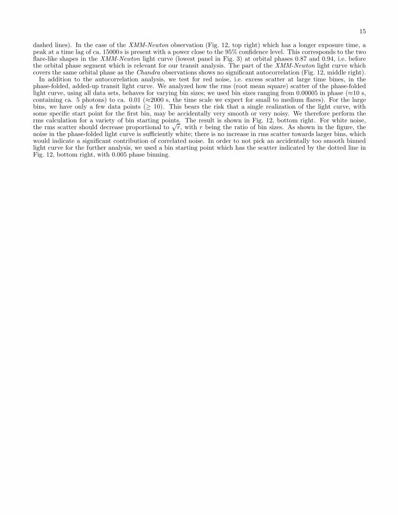
The host star HD 189733A is an active cool star, so that one may expect flares to occur in the stellar corona. Ifmajor flaring events are present, the sequence of measured X-ray photons per time bin will not be random, but willdisplay autocorrelation. If autocorrelation is present at significant levels, a more detailed treatment of the errors inthe phase-folded light curve has to be performed. We therefore compute the autocorrelation function of each X-raylight curve, using time bins of 200 s as shown in Fig. 3, left and top right.

−0.4

0.0

0.4Chandra 1

−0.4

0.0

0.4Chandra 2

−0.4

0.0

0.4Chandra 3

−0.4

0.0

0.4

auto

corr

ela

tion f

unct

ion

Chandra 4

−0.4

0.0

0.4Chandra 5

0 5000 10000 15000 20000time lag (s)

−0.4

0.0

0.4Chandra 6

Fig. 12.— Left: Autocorrelation function for the individual Chandra light curves binned by 200 s. Top right: Autocorrelation functionfor the XMM-Newton light curve binned by 200 s, for the complete length of the observation (top) and for the time interval close to thetransit (middle, dotted lines in Fig. 3). The dashed lines represent the 95% confidence levels for autocorrelation. Bottom right: The rmsscatter of the phase-folded X-ray light curve for different bin sizes. The different symbols depict different binning start points, which causea spread in scatter at larger bin sizes. The expected slope for white noise is depicted by the arrow. The dotted line depicts the rms of thelight curve in Fig. 8 at different bin sizes; the final phase binning in Fig. 8 is 0.005.

We show the result in Fig. 12 (left) for the Chandra light curves. While there is some slight modulation visiblein some of the autocorrelation plots, it does not reach a significant level (95% confidence threshold depicted by the

15

dashed lines). In the case of the XMM-Newton observation (Fig. 12, top right) which has a longer exposure time, apeak at a time lag of ca. 15000 s is present with a power close to the 95% confidence level. This corresponds to the twoflare-like shapes in the XMM-Newton light curve (lowest panel in Fig. 3) at orbital phases 0.87 and 0.94, i.e. beforethe orbital phase segment which is relevant for our transit analysis. The part of the XMM-Newton light curve whichcovers the same orbital phase as the Chandra observations shows no significant autocorrelation (Fig. 12, middle right).In addition to the autocorrelation analysis, we test for red noise, i.e. excess scatter at large time bines, in the

phase-folded, added-up transit light curve. We analyzed how the rms (root mean square) scatter of the phase-foldedlight curve, using all data sets, behaves for varying bin sizes; we used bin sizes ranging from 0.00005 in phase (≈10 s,containing ca. 5 photons) to ca. 0.01 (≈2000 s, the time scale we expect for small to medium flares). For the largebins, we have only a few data points (≥ 10). This bears the risk that a single realization of the light curve, withsome specific start point for the first bin, may be accidentally very smooth or very noisy. We therefore perform therms calculation for a variety of bin starting points. The result is shown in Fig. 12, bottom right. For white noise,the rms scatter should decrease proportional to

√r, with r being the ratio of bin sizes. As shown in the figure, the

noise in the phase-folded light curve is sufficiently white; there is no increase in rms scatter towards larger bins, whichwould indicate a significant contribution of correlated noise. In order to not pick an accidentally too smooth binnedlight curve for the further analysis, we used a bin starting point which has the scatter indicated by the dotted line inFig. 12, bottom right, with 0.005 phase binning.