transient solutions for three-dimensional lid-driven cavity …frey/papers/navier-stoke… · ·...

INTERNATIONAL JOURNAL FOR NUMERICAL METHODS r~ FLUIDS, VOL. 2 1,413432 (1995)

TRANSIENT SOLUTIONS FOR THREE-DIMENSIONAL LID-DRIVEN CAVITY FLOWS BY A LEAST-SQUARES

FINITE ELEMENT METHOD LI Q. TANG,* TIWU CHENGt AND TATE T. H. TSANGt

Department of Chemical and Materials Engineering, University of Kentucky, Lexington, KY 40506-0046, I/;S.A.

SUMMARY

A time-accurate least-squares finite element method is used to simulate three-dimensional flows in a cubic cavity with a uniform moving top. The time- accurate solutions are obtained by the Crank-Nicolson method for time integration and Newton linearization for the convective terms with extensive linearization steps. A matrix-free algorithm of the Jacobi conjugate gradient method is used to solve the symmetric, positive definite linear system of equations. To show that the least-squares finite element method with the Jacobi conjugate gradient technique has promising potential to provide implicit, fully coupled and time-accurate solutions to large-scale three-dimensional fluid flows, we present results for three-dimensional lid-driven flows in a cubic cavity for Reynolds numbers up to 3200.

KEY WORDS: least-squares finite element method; Jacobi conjugate gradient method; three-dimensional flows; time-accurate solutions; lid-driven flows

1. INTRODUCTION

The flow of an incompressible fluid in a square cavity, driven by the moving top at a uniform velocity, has served as a benchmark problem to validate various numerical techniques for two-dimensional fluid flow^.'^ The interest of the problem is due to its simple geometry and Dirichlet boundary conditions. However, numerical results for three-dimensional driven cavity flows are relatively scarce. Unlike two- dimensional lid-dnven cavity flows, flows in a cubic cavity are rich in complicated physical phenomena. Moreover, an increase in the number of unknowns drastically increases the memory requirement for the numerical solution of the resulting linear system of equations by direct methods. It also has, in general, an adverse effect on the rate of convergence of most iterative methods. Therefore difficulties, primarily due to prohibitive computing cost and limitations on computing capabilities, arise when a large number of unknowns are required for accurate numerical solutions of three- dimensional flows.

Earlier simulations of three-dimensional lid-driven flows in a cubic cavity were for low-Reynolds- number flows' and results were obtained with inadequate resolutions because of limited computing resource^.^'^ More recently, Guj and Stella' used an AD1 finite difference method for steady state flows for 400 < Re < 2000 based on the vorticity-velocity formulation of the Navier-Stokes equations with staggered grids varied from 3 1 x 31 x 16 to 101 x 101 x 41 points. Iwatsu et al.9 used a time- marching MAC method for unsteady state flows at Re = 2000 and 4000. The time step was taken as

Permanent address: Center for Computational Sciences, University of Kentucky, Lexington, KY 40506-0045, U.S.A. Permanent address: Department of Basic Sciences, China Textile University, Shanghai, People's Republic of China.

f Author to whom correspondence should be addressed.

CCC 027 1-2091/95/050413-20 0 1995 by John Wiley & Sons, Ltd.

Received 7 September 1994 Revised 4 Janualy 1995

414 L. Q. TANG, T. CHENG AND T. T. H. TSANG

At = 1 O r ' and the number of grid points was 8 1 x 8 1 x 8 1. The loss of flow symmetry was observed for Re = 4000. Direct solutions for unsteady incompressible flows using the velocity-vorticity formulation were obtained by Osswald et al." The vorticity transport equation was solved by a modified AD1 method. The direct, implicit algorithm was tested for the case of Re = 100 with a mesh system of 17 x 17 x 17 grid points.

Ku et al." employed a Chebyshev pseudospectral method for unsteady state flows for 100 < Re < 1000 based on primitive variables by using a time-splitting technique with a grid of 3 1 x 3 1 x 16 points. Time steps of At = 5 x 1 0-4 and 7 x 1 0-4 were used and it took 750&25,000 time steps to obtain the steady state solutions.

It is well known that for both steady state and time-dependent problems using an implicit solution approach, most finite element methods lead to a large sparse unsymmetric linear system which is difficult to solve numerically. The steady state lid-driven cavity flows for 100 < Re < 400 based on the vorticity-velocity formulation of the compressible Navier-Stokes equations were simulated by Guevremont et al. l2 using a weak Galerkin finite element method followed by Newton linearization. Three grid systems were used: two coarse grids of 8 x 8 x 4 and 14 x 14 x 7 elements by a direct solver and a finer grid of 30 x 30 x 15 elements by an iterative solver based on an Arnoldi method. Kato et al." proposed a GSMAC finite element method which uses mass lumping to reduce the memory requirement. The unsteady state flows based on a first-order velocity-vorticity-Bernoulli function formulation were solved for Re < 3200. The grid composed 40 x 40 x 20 elements. Fujima et al. l4 reported transient solutions for Re < 2000 by an upwind finite element method based on the choice of upwind and downwind points. The explicit Euler method in time was used for the Navier-Stokes equations and the pressure Poisson equation was solved by an incomplete Cholesky conjugate gradient method. The flow domain was divided into 20 x 20 x 10 non-uniform bricks with six tetrahedra for each brick.

More recently a least-squares finite element method (LSFEM) has been developed to solve steady state incompressible flows in a cubic cavity by Jiang et at Re = 100, 400 and 1000 for a mesh system of 50 x 52 x 25 elements. In addition, Jiang et al.l6 presented a detailed theoretical analysis of incompressible Navier- Stokes problems by the LSFEM. They proved that the three-dimensional div-curl system resulting from the LSFEM is properly determined and elliptic and established the existence and uniqueness of the least-squares finite element solution of the system.

Our goal is to develop an accurate, implicit and robust algorithm of the LSFEM to simulate three- dimensional transient flow problems. Particular attention is given to the following approaches.

1. An implicit, fully coupled and time-accurate solution is obtained in terms of a first-order velocity-pressure-vorticity formulation.

2. Temporal discretization of the Navier-Stokes equations is implemented by the Crank-Nicolson method with second-order accuracy in time.

3. The non-linear convective terms are linearized by Newton's method with extensive linearization steps.

4. Spatial discretization of the Navier-Stokes equations is based on the LSFEM to obtain a symmetric, positive definite linear system of equations.

5. The resulting symmetric, positive definite linear system of equations is solved by a matrix-free Jacobi conjugate gradient method (JCG) without forming any global matrix, not even an element matrix.

6. Trilinear hexahedral elements with equal-order interpolation functions are used for all variables. 7. Both uniform and non-uniform meshes are employed up to 60 x 61 x 30 elements.

The content of the paper is organized as follows. In Section 2 we give a brief account of the first- order velocity-pressure-vorticity formulation, compatibility constraint and initial and boundary

3D LID-DRIVEN CAVITY FLOWS 415

conditions. In Section 3 numerical results of three-dimensional lid-dnven cavity flows for Re = lo& 3200 are presented and discussed. The conclusions are given in Section 4.

2. FORMULATION

2. I . Governing equations

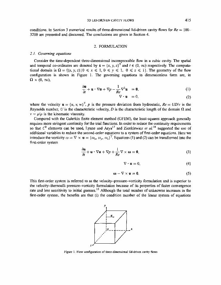
Consider the time-dependent three-dimensional incompressible flow in a cubic cavity. The spatial and temporal co-ordinates are denoted by x = {x, y, z } ~ and t E (0, 00) respectively. The computational domain is rZ = {(x, y, z) 1 0 < x < 1, 0 < y < 1, 0 < z < 1). The geometry of the flow configuration is shown in Figure 1. The governing equations in dimensionless form are, in l-2 x (0, 001,

au 1 at Re -+ u * vu + vp - -v2u = 0,

v - u = o , where the velocity u = { u , v, w } ~ , p is the pressure deviation from hydrostatic, Re = UDIv is the Reynolds number, U is the characteristic velocity, D is the characteristic length of the domain R and v = plp is the kinematic viscosity.

Compared with the Galerkin finite element method (GFEM), the least-squares approach generally requires more stringent continuity for the trial functions. In order to reduce the continuity requirements so that and Zienkiewicz et a1." suggested the use of additional variables to reduce the second-order equations to a system of first-order equations. Here we introduce the vorticity w = V x u = { w,, a,,, w , } ~ . Equations (1) and ( 2 ) can be transformed into the first-order system

elements can be used, Lynne and

au 1 at Re - + u * v u + vp + -v x w = 0, ( 3 )

w - v x u = o . (5)

This first-order system is referred to as the velocity-pressure-vorticity formulation and is superior to the velocity-Bernoulli pressure-vorticity formulation because of its properties of faster convergence rate and less sensitivity to initial guesses." Although the total number of unknowns increases in the first-order system, the benefits are that (i) the condition number of the linear system of equations

t Y

Figure 1. Flow configuration of three-dimensional lid-driven cavity flows


discretized by the LSFEM can be reduced from O(h-4)'9 to O(h-2),20 (ii) a simple piecewise linear C? element can be used, (iii) unlike the GFEM, the choice of approximating spaces is not subject to the LBB condition,2' so that equal-order interpolation functions can be employed for all variables, and (iv) the resulting matrix system is symmetric, positive definite.

For the three-dimensional problem the first-order system involves an odd number of unknowns (seven) and an odd number of equations and cannot form an elliptic system." Therefore we use a constraint (the solenoidality of vorticity)

V - o = O i n n .

The constraint (6) is a very important condition to be enforced in some way in three-dimensional problems when the vorticity is introduced as an unknown. First, it provides an optimal rate of convergence for all variables in the LSFEM.I5.l6 Second, it forces V-w(x, t) to approach zero as t goes to infinity if a non-physical initial condition, leading to V*o(x, t = 0) # 0, is used.' On the other hand, if V w = 0 initially, it will remain so throughout the computation, since a(V.o)/at = 0. Third, the constraint (6) gives an explicit relationship and sets up a physical balance between the vorticity components. Otherwise the vorticity components would implicitly be related by the rotation tensor and the solutions of vorticity may oscillate even at Gaussian points, as will be shown later. For two- dimensional problems the vorticity component exists only in the direction normal to the plane and equation (6) is automatically satisfied. It is worth mentioning that the matrix resulting from the least- squares approximation has a structure like [A] = [A]' [A]. The transpose of a non-square matrix [dl maps itself in Weq, x Ndof to a matrix [dl in W " o f Ndof, where N~~~ is the number of equations, Ndof is the number of degrees of freedom and Neqs 2 Ndof. Therefore the additional equation (6) does not increase the total number of unknowns in the system.

2.2. Time discretization and linearization

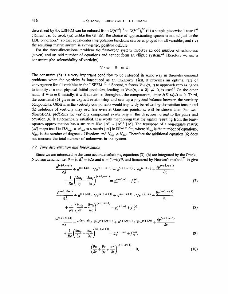
Since we are interested in the time-accurate solutions, equations (3H6) are integrated by the Cranl- Nicolson scheme, i.e. 8 = i, A? = t9At and 8 = (1--8)/0, and linearized by Newton's method23 to give

u(n+l ,m+l) m+l) + U(n+I.m) . Vu(n+l.m+l) + U(n+lm+l) . v,(n+l,m)

A i + ax

3D LID-DRIVEN CAVITY FLOWS

and

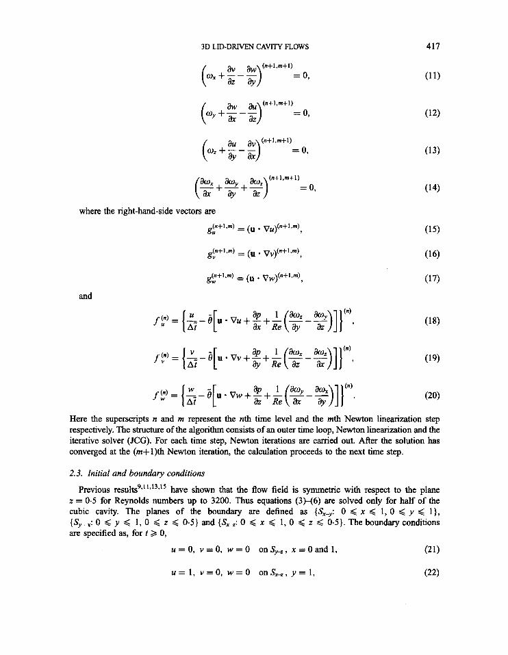
Here the superscripts n and m represent the nth time level and the mth Newton linearization step respectively. The structure of the algorithm consists of an outer time loop, Newton linearization and the iterative solver (JCG). For each time step, Newton iterations are carried out. After the solution has converged at the (m+l)th Newton iteration, the calculation proceeds to the next time step.

2.3. Initial and boundary conditions

Previous results9” 1*13~15 have shown that the flow field is symmetric with respect to the plane z = 0.5 for Reynolds numbers up to 3200. Thus equations (3H6) are solved only for half of the cubic cavity. The planes of the boundary are defined as {Sx-y: 0 < x < 1, 0 < y < l} , {S , x: 0 < y < 1, 0 < z < 0.5) and {SX-=: 0 < x < 1 , O < z < 0.5). The boundary conditions are specified as, for t 2 0,

u = O , v = O , w = O on&, x = O a n d l , (21)

u = 1 . v = O , w = O onS,,, y = 1 , (22)


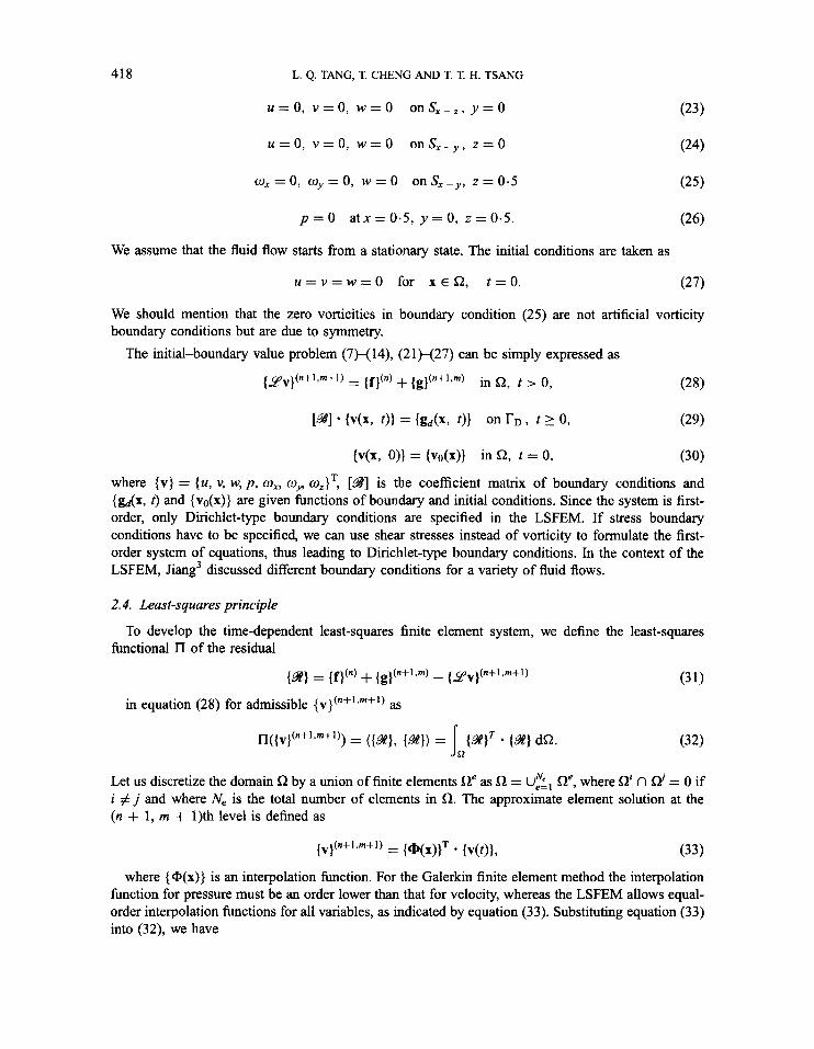
u = O , v=O, w = O onS,_., y = O (23)

u = O , v = O , w = O onS,-,, z = O (24)

o , = O , o y = O , w = O onS,-,, z=O.5 (25)

p = O atx=O.5, y = O , z = 0 . 5 . (26)

We assume that the fluid flow starts from a stationary state. The initial conditions are taken as

u = v = w = O for X E Q , t = 0 . (27)

We should mention that the zero vorticities in boundary condition (25) are not artificial vorticity boundary conditions but are due to symmetry.

The initial-boundary value problem (7H14), (21H27) can be simply expressed as

(28) { z v ) ( n + l . m + l ) - - (f)(n) + {gj(n+l.m) in 0, , 0,

{v(x, 0)) = {vo(x)} in Q, t = 0, (30)

where {v} = {u, v, w, p , ox, or u.}~, [&?I is the coefficient matrix of boundary conditions and { d x , t ) and {vo(x)} are given functions of boundary and initial conditions. Since the system is first- order, only Dirichlet-type boundary conditions are specified in the LSFEM. If stress boundary conditions have to be specified, we can use shear stresses instead of vorticity to formulate the first- order system of equations, thus leading to Dirichlet-type boundary conditions. In the context of the LSFEM, Jiang3 discussed different boundary conditions for a variety of fluid flows.

2.4. Least-squares principle

functional ll of the residual To develop the time-dependent least-squares finite element system, we define the least-squares

Let us discretize the domain R by a union of fmite elements Re as R = Uf:l Re, where Qi n N = 0 if i # j and where N, is the total number of elements in Q. The approximate element solution at the (n + 1, m + 1)th level is defined as

(33) { , ) (n+lm+l) - - * Iv(t)),

where { @(x)} is an interpolation function. For the Galerkin finite element method the interpolation function for pressure must be an order lower than that for velocity, whereas the LSFEM allows equal- order interpolation functions for all variables, as indicated by equation (33). Substituting equation (33) into (32), we have


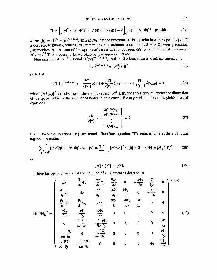
{ v } ~ - [9{@}IT * [9{@}] - {v} dC2 - 2 { v } ~ * [9{@}lT - (b} d@, (34) J* where {b} = {f}(")+{g}~"+""'. This shows that the functional l7 is a quadratic with respect to {v}. It is desirable to know whether ll is a minimum or a maximum at the point 6n = 0. Obviously equation (34) requires that the sum of the squares of the residual of equation (28) be a minimum at the correct solution.24 This process is the well-known least-squares method.

Minimization of the functional n( { ~ } ( " + l , ~ + l ) ) leads to the least-squares weak statement: find

{V}(n+l.m+l) E [&'f@)ld (35)

such that

where [&';(!2)ld is a subspace of the Sobolev space [&'.'(!2)ld, the superscript d denotes the dimension of the space and N, is the number of nodes in an element. For any variation 6{v} this yields a set of equations

fiom which the solutions {vi} are found. Therefore equation (37) reduces to a system of linear algebraic equations

or

[XI * { V } = (91, where the operator matrix at the ith node of an element is denoted as

av - ai ax

dvi

av - ai az aai ay

1 aai ~

_- Re az

0

1 aai Re ax

aai aai ax az

~ 0 --

0 ai 0

0 0 mi

0 0 0

0

0

0 0

0 0

aa1 0 - ax

aai 0 -

?Y aai ai - az

aai ?Y aai ax

~

--

420

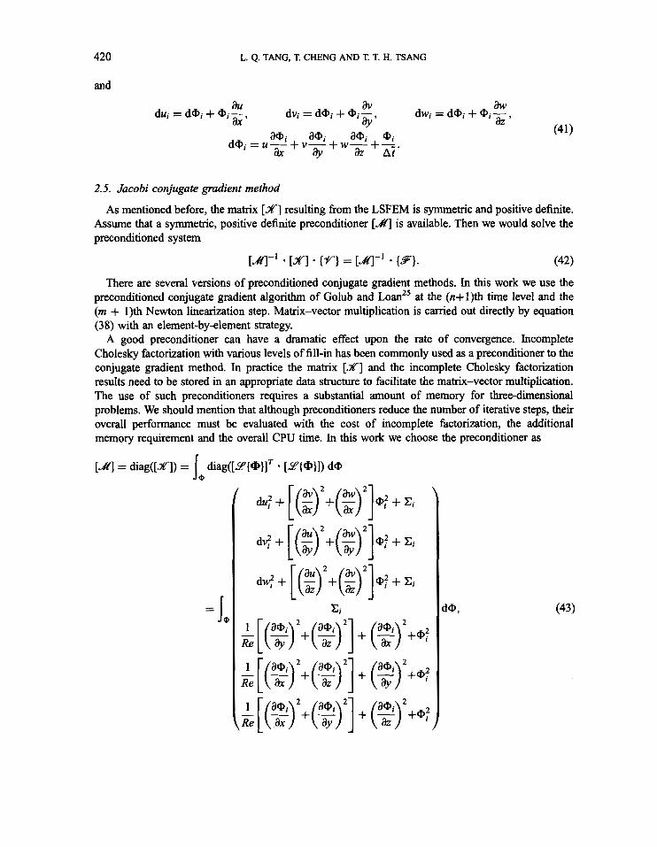
and

L. Q. TANG, T. CHENG AND T. T. H. TSANG

2.5. Jacobi conjugate gradient method

As mentioned before, the matrix [XI resulting from the LSFEM is symmetric and positive definite. Assume that a symmetric, positive definite preconditioner [MI is available. Then we would solve the preconditioned system

[MI-' * [XI (V} = [MI-* * (S}. (42)

There are several versions of preconditioned conjugate gradient methods. In this work we use the preconditioned conjugate gradient algorithm of Golub and Loanz5 at the (n+l)th time level and the (m + 1)th Newton linearization step. Matrix-vector multiplication is carried out directly by equation (38) with an element-by-element strategy.

A good preconditioner can have a dramatic effect upon the rate of convergence. Incomplete Cholesky factorization with various levels of fill-in has been commonly used as a preconditioner to the conjugate gradient method. In practice the matrix [XI and the incomplete Cholesky factorization results need to be stored in an appropriate data structure to facilitate the matrix-vector multiplication. The use of such preconditioners requires a substantial amount of memory for three-dimensional problems. We should mention that although preconditioners reduce the number of iterative steps, their overall performance must be evaluated with the cost of incomplete factorization, the additional memory requirement and the overall CPU time. In this work we choose the preconditioner as

[ d l = diag([Xl) = I diag([u{@llT * [27(@H) d@ J @

= J, & [ (EJ2+(EJ2] + (!.%)2+@:

Re L [ ("a32+(?.3)2] - + (!3)2+@; 2- [ (32+(32] + (x) aai +@;

Re

(43)

3D LID-DRTVEN CAVITY FLOWS 42 1

where

x.- I - (EJ2 + - (a;>' + - (a;j2 Therefore it is a Jacobi conjugate gradient method. Pini and Gambolati26 found that simple diagonal scaling or the Jacobi conjugate gradient method is an efficient preconditioning scheme for a variety of applications. It is necessary to emphasize that the Jacobi preconditioner is simple and easy to code. It does not require the formation of any global matrix, not even an element matrix. Such a matrix-free approach leads to tremendous savings in computer memory and computing time?'

3. RESULTS AND DISCUSSION

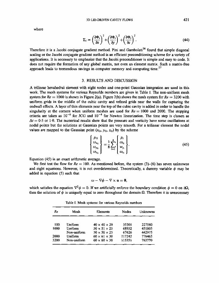
A trilinear hexahedral element with eight nodes and one-point Gaussian integration are used in this work. The mesh systems for various Reynolds numbers are given in Table I. The non-uniform mesh system for Re = 1000 is shown in Figure 2(a). Figure 2(b) shows the mesh system for Re = 3200 with uniform grids in the middle of the cubic cavity and refined grids near the walls for capturing the endwall effects. A layer of thin elements near the top of the cubic cavity is added in order to handle the singularity at the corners when uniform meshes are used for Re = 1000 and 2000. The stopping criteria are taken as for Newton linearization. The time step is chosen as At = 0.5 or 1.0. The numerical results show that the pressure and vorticity have some oscillations at nodal points but the solutions at Gaussian points are very smooth. For a trilinear element the nodal values are mapped to the Gaussian point (XG, YG, zG) by the scheme

for JCG and

' . (45)

Equation (45) is an exact arithmetic average. We first test the flow for Re = 100. As mentioned before, the system (3)-(6) has seven unknowns

and eight equations. However, it is not overdetermined. Theoretically, a dummy variable 4 may be added in equation ( 5 ) such that

w - v4 - v x u =o , which satisfies the equation V2$ = 0. If we artificially enforce the boundary condition $ = 0 on 82, then the solution of 4 is uniquely equal to zero throughout the domain a. Therefore it is unnecessary

Table I. Mesh systems for various Reynolds numbers

Re Mesh Elements Nodes Unknowns

100 Uniform 40 x 40 x 20 35301 227580 1000 Uniform 50 x 51 x 25 68952 45 1803

Non-uniform 50 x 50 x 25 67626 442975 2000 Uniform 60 x 61 x 30 117242 776463 3200 Non-uniform 60 x 60 x 30 115351 763770


Figure 2. Non-uniform mesh grids for (a) Re = 1000 and (b) Re = 3200

to add the dummy variable in system (3H6). Detailed discussion was given by Jiang et a1." Our numerical results show that 4 is not equal to zero but its maximum magnitude is quite small, about 0(10-*) near the boundary and 0(10-") inside the domain when the stopping criterion of JCG is taken to be The values of the dummy variable are so small that its existence does not affect the numerical solutions.

1.0 1.0

0.0 0.0

0.0 0.0

0.4 0.4

ol14=?&4 0.0 0.0 0.8 0.4 0.0 0.0 1.0

0.0 0.2 0.4 0.0 0.0 1.0

I"-", 0.2 0.4 0.0 0.0 1.0

1.0

0.0

0.0

0.4

0.2 X

t 0.0 0.2 0.4 0.0 0.0 1.0

1.0 1.0

0.0 0.0

0.6 0.0

0.4 0.4

0.8 0.8

0.0 b x 0.0 0.8 0.4 0.0 0.8 1.0 0.2 0.4 0.0 0.0 1.0

Z (4 (b)

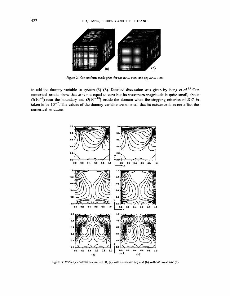
Figure 3. Vorticity contours for Re = 100, (a) with constraint (6) and (b) without constraint (6)


Table 11. Computer memory requirements and CPU times on an HP-735 workstation

Reynolds Number of Stopping Time Storage CPU time number elements time steps (Mb) 01)

100 40 x 40 x 20 8 16 21 2.5 1000 50x51 x 2 5 50 75 54 51.3 2000 60 x 61 x 30 110 160 92 128.6

To show the importance of constraint (6), we simulate the flow for Re = 100 for two cases, with and without constraint (6). The vorticity contours on the planes z = 0.5, y = 0.5, x = 0.5 are shown in Figure 3. Both results are smoothed at the Gaussian point of each element by equation (45). The solutions with constraint (6) are very smooth as shown in Figure 3(a). However, without constraint (6) the vorticity components w,, and w, on the planes y = 0.5, z = 0.5 oscillate along the walls as shown in Figure 3(b). This indicates that constraint (6) is a very important condition to be enforced in three- dimensional flow problems when vorticity is introduced as an unknown. On the other hand, numerical results also show that the values of velocity and pressure do not differ significantly between the two cases. This implies that constraint (6) hardly disturbs the velocity and pressure fields.

The CPU time for Re = 100 is about 2.5 h on an HP-735 workstation (CONVEX MetaSystem) and 8 . 5 h on an IBM 3090-6005 computer. The simulation requires 27 Mb of computer memory. The memory requirements and computing times are given in Table I1 for various Reynolds numbers.

t - 5 t = 1 0

t = 20 -x t = 30 t = 5in

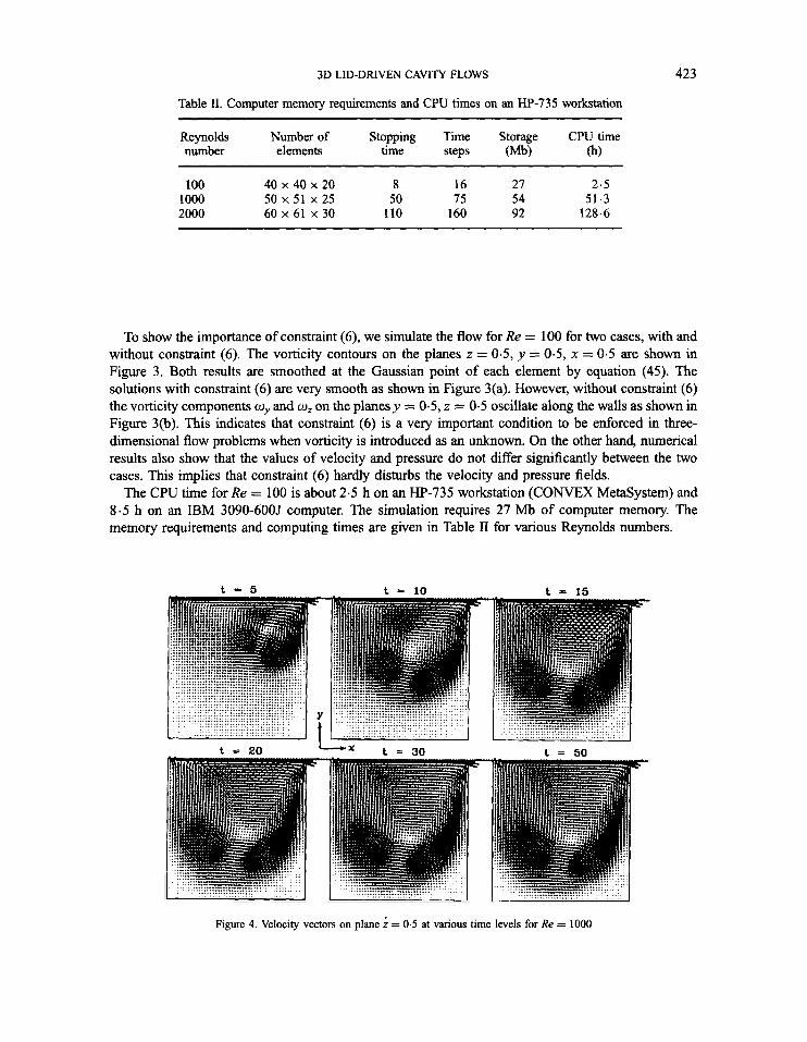
Figure 4. Velocity vectors on plane = 0.5 at various time levels for Re = 1000


3.1. Numerical results for Re = I000

The transient solutions for Re = 1000 are obtained at time levels t = 5 , 10, 15, 20, 30, 50. The velocity vectors by the uniform mesh on the planes x = 0-5, y = 0.5, z = 0.5 are presented in Figures 4-6. Figure 4 shows that a primary vortex appears near the right corner of the top wall at the beginning and moves to the location at about x = 0.60, y = 0.45, similarly to the two-dimensional flow problem.

t - 5

t = 20

t - 10 t I 16

I' t = 30 t = 50

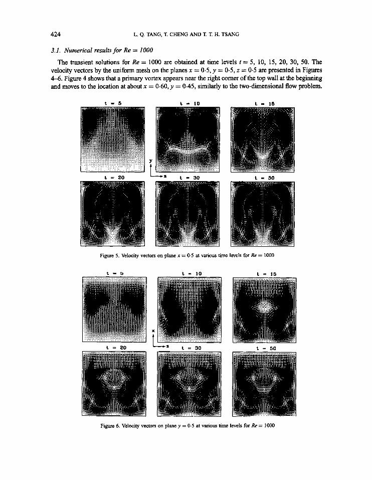
Figure 5. Velocity vectors on plane x = 0.5 at various time levels for Re = 1000

t = S

t = 20

t = 10 t = 15

X

t I' t = 30 L = 50

Figure 6. Velocity vectors on plane y = 0.5 at various time levels for Re = 1000


-1 4.8 4.6 4.4 02 0 0.2 0.4 0.8 0.8 1 wdody

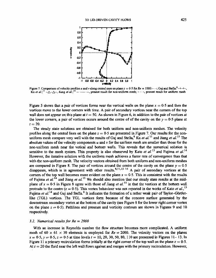
Figure 7. Comparison of velocity profiles Y and v along central axes on plane z = 0.5 for Re = IOOO:-; Guj and Stella;8-+-+-, Ku et aL;" -A-A-, Jiang et aL;" ___ , present result for non-uniform mesh; - - -, present result for uniform mesh

Figure 5 shows that a pair of vortices forms near the vertical walls on the plane x = 0.5 and then the vortices move to the lower comers with time. A pair of secondary vortices near the comers of the top wall does not appear on this plane at t = 50. As shown in Figure 6, in addition to the pair of vortices at the lower comers, a pair of vortices occurs around the centre of of the cavity on the y = 0.5 plane at t = 20.

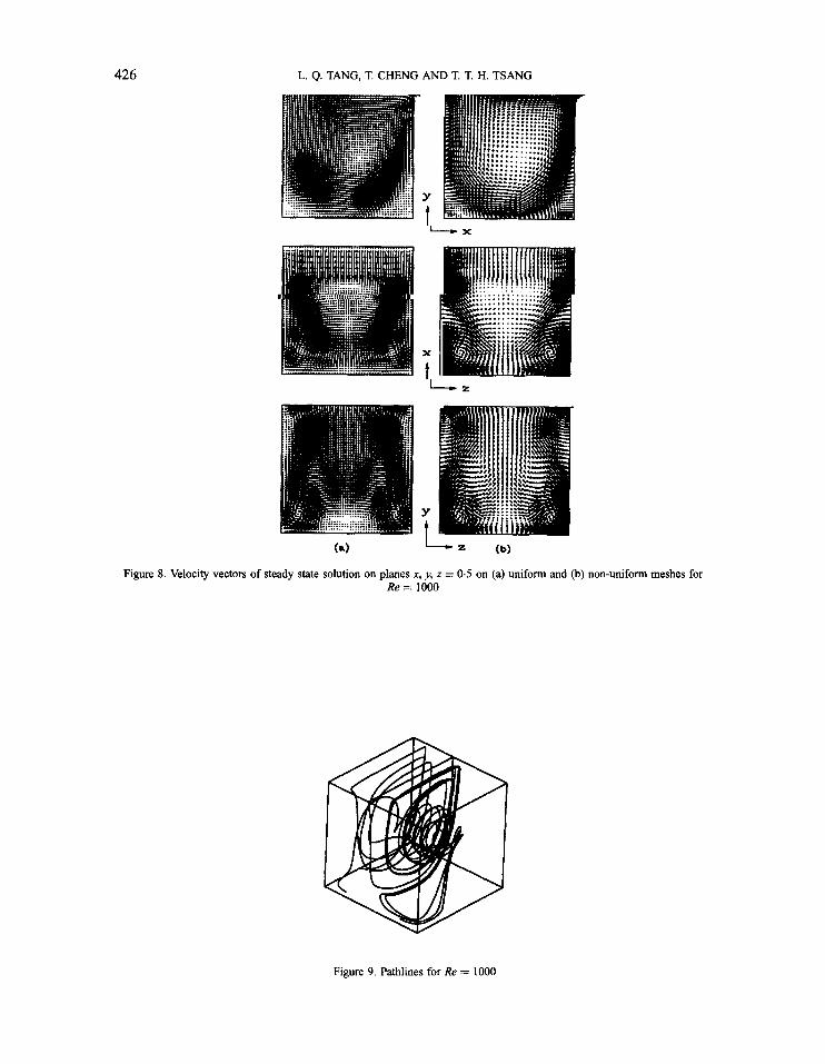
The steady state solutions are obtained for both uniform and non-uniform meshes. The velocity profiles along the central lines on the plane z = 0.5 are presented in Figure 7. Our results for the non- uniform mesh compare very well with the results of Guj and Stella,' Ku et al." and Jiang et al. l5 The absolute values of the velocity components u and v for the uniform mesh are smaller than those for the non-uniform mesh near the vetical and bottom walls. This reveals that the numerical solution is sensitive to the mesh system. This property is also obsesrved by Kato et ~ 1 . ' ~ and Fujima et However, the iterative solution with the uniform mesh achieves a faster rate of convergence than that with the non-uniform mesh. The velocity vectors obtained from both uniform and non-uniform meshes are compared in Figure 8. The pair of vortices around the centre of the cavity on the plane y = 0-5 disappears, which is in agreement with other re~ults.'"','~-'~ A pair of secondary vortices at the comers of the top wall becomes more evident on the plane x = 0.5. This is consistent with the results of Fujima et and Jiang et al." We should also mention that our steady state results at the mid- plane of x = 0.5 in Figure 8 agree with those of Jiang et ul? in that the vortices at the bottom wall protrude to the centre (z = 0-5). This vortex behaviour was not reported in the works of Kato et al.,I3 Fujima et al. l4 and Guj and Stella.' It indicates the formation of a rather weak pair of Taylor4ortler- like (TGL) vortices. The TGL vortices form because of the concave surface generated by the downstream secondary vortex at the bottom of the cavity (see Figure 8 for the lower right comer vortex on the plane z = 0-5). Pathlines and pressure and vorticity contours are shown in Figures 9 and 10 respectively.

3.2. Numerical results for Re = 2000

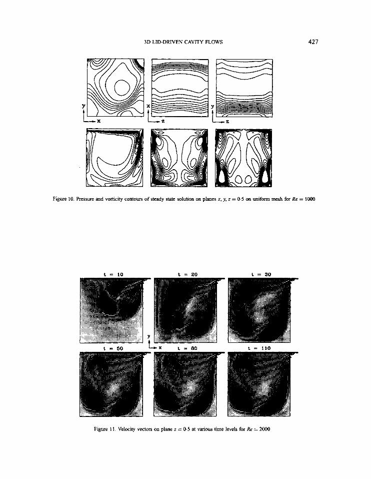
With an increase in Reynolds number the flow structure becomes more complicated. A uniform mesh of 60 x 61 x 30 elements is employed for Re = 2000. The velocity vectors on the planes x = 0-5, y = 0.5, z = 0-5 at time levels t = 10,20,30, 50,80, 110 are presented in Figures 11- 13. In Figure 1 1 a primary recirculation forms initially at the right comer of the top wall on the plane z = 0.5. At t = 20 the fluid near the left wall flows against and merges with the primary recirculation. However,


Y

t Figure 8. Velocity vectors of steady state solution on planes x , y, z = 0.5 on (a) uniform and (b) non-uniform meshes for

Re = 1000

Figure 9. Pathlines for Re = 1000

Y t I X

427 3D LID-DRIVEN CAVITY FLOWS

I

Figure 10. Pressure and vorticity contours of steady state solution on planes x, y, z = 0.5 on uniform mesh for Re = 1000

t = 10 t = 20 t = 30

t P 50 L X t = ao t = 1 1 0

Figure 1 1 . Velocity vectors on plane z = 0.5 at various time levels for Re = 2000


t = 10 t = 20 t t sn

t = 60 t = 80 t I 11n

Figure 12. Velocity vecton 011 plane y = 0.5 at Various time levels for Re = 2000

t I I 0

Y

t

t = 20 t a 30

t = 110 - D z t = 80

Figure 13. Velocity vectors on plane x = 0.5 at various time levels for Re = 2000


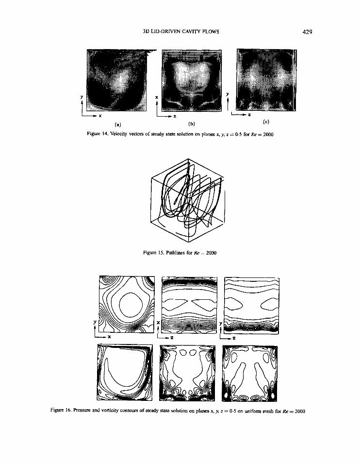
(b) ( c ) (4 Figure 14. Velocity vectors of steady state solution on planes x, y, z = 0.5 for Re = 2000

Figure 15. Pathlines for Re = 2000

Figure 16. Pressure and vorticity contours of steady state solution on planes x, y, z = 0.5 on uniform mesh for Re = 2000


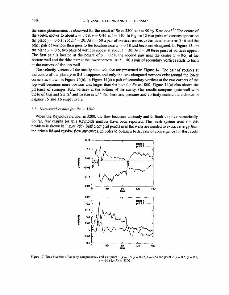
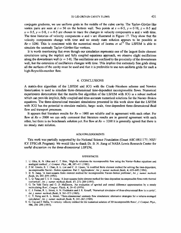
the same phenomenon is observed for the result of Re = 3200 at t = 90 by Kato et al. l 3 The centre of the vortex moves to about x = 0.58, y = 0.46 at t = 110. In Figure 12 two pairs of vortices appear on the plane y = 0.5 at about t = 20. At t = 50 a pair of vortices moves to the location at x = 0.46 and the other pair of vortices then goes to the location near x = 0- 18 and becomes elongated. In Figure 13, on the plane x = 0.5, two pairs of vortices appear at about t = 20. At t = 30 three pairs of vortices appear. The first pair is located at the height of y = 0.58, the second pair near the centre (z = 0.5) at the bottom wall and the third pair at the lower comers. At t = 80 a pair of secondary vortices starts to form at the corners of the top wall.

The velocity vectors of the steady state solution are presented in Figure 14. The pair of vortices at the centre of the plane y = 0.5 disappears and only the two elongated vortices exist around the lower comers as shown in Figure 14(b). In Figure 14(c) a pair of secondary vortices at the two comers of the top wall becomes more obvious and larger than the pair for Re = 1000. Figure 14(c) also shows the presence of stronger TGL vortices at the bottom of the cavity. Our results compare quite well with those of Guj and Stella* and Iwatsu et ~ 1 . ~ Pathlines and pressure and vorticity contours are shown in Figures 15 and 16 respectively.

3.3. Numerical results for Re = 3200

When the Reynolds number is 3200, the flow becomes unsteady and difficult to solve numerically. So far, few results for this Reynolds number have been reported. The mesh system used for this problem is shown in Figure 2(b). Sufficient grid points near the walls are needed to extract energy fiom the driven lid and resolve flow structures. In order to obtain a better rate of convergence for the Jacobi

0.18 point1 - point 2

0.1 - 9 n -, point 2

..# ..._ _.__ v. .............................. -4. ......... y I ......................... /""Y"il ............... L 'j ;I ;q\ ; \,! :: 1 '-\-.+-.

I 0 40 80 120 180

Urn0

0.25 - point1 - polnt2 -

4.05 - 4.1

0 40 80 120 160 Urn0

Figure 17. Time histories of velocity components I( and v at point 1 (x = 0.5, y = 0.1 8, z = 0.5) and point 2 (x = 0.5, y = 0.8, z = 0.5) for Re = 3200

3D LID-DRIVEN CAVITY FLOWS 43 1

conjugate gradients, we use uniform grids in the middle of the cubic cavity. The Taylor-Gortler-like vortex pairs are seen at t = 50 on the bottom wall. Two points at x = 0-5, y = 0.18, z = 0.5 and x = 0.5, y = 0.8, z = 0.5 are chosen to trace the changes in velocity components u and v with time. The time histories of velocity components u and v are illustrated in Figure 17. They show that the velocity components change with time and no steady state solution appears to be possible at Re = 3200. This is consistent with the numerical result of Iwatsu et al.9 The LSFEM is able to simulate the unsteady Taylor-Gortler-like vortices.

It is worth mentioning that even though our simulation represents one of the largest finite element simulations using the implicit and fully coupled equations approach, we observe slight oscillations along the downstream wall (x = 1 .O). The oscillations are confined to the proximity of the downstream wall, but the extension of oscillations changes with time. This implies that extremely fine grids along all the surfaces of the cavity must be used and that it is preferable to use non-uniform grids for such a high-Reynolds-number flow.

4. CONCLUSIONS

A matrix-free algorithm of the LSFEM and JCG with the Crank-Nicolson scheme and Newton linearization is used to simulate three-dimensional time-dependent incompressible flows. Numerical experiments demonstrate that the matrix-free algorithm of the LSFEM with JCG is a robust method which can provide implicit, fully coupled and time-accurate numerical solutions for the Navier-Stokes equations. The three-dimensional transient simulations presented in this work show that the LSFEM with JCG has the potential to simulate realistic, large- scale, time-dependent three-dimensional fluid flow and transport processes.

It appears that literature results for Re = 1000 are reliable and in agreement with each other. For flow at Re = 2000 we can only comment that literature results are in general agreement with each other, but there is no benchmark solution yet. For flow at Re = 3200 it is generally agreed that there is no steady state solution.

ACKNOWLEDGEMENTS

This work was partially supported by the National Science Foundation (Grant ASC-88 1 1 17 1 ; NSF/ KY EPSCoR Program). We would like to thank Dr. B. N. Jiang of NASA Lewis Research Center for useful discussion on the three-dimensional LSFEM.

REFERENCES

1. U. Ghia, K. N. Ghia and C. T. Shin, ‘High-Re solutions for incompressible flow using the Navier-Stokes equations and

2. F? M. Gresho, S. T. Chan, R. L. Lee and C. D. Upson, ‘A modified finite element method for solving the time-dependent,

3. B. N. Jiang, ‘A least-squares finite element method for incompressible Navier-Stokes problems’, Int. j . numer: methods

4. L. Q. Tang and T. T. H. Tsang, ‘A least-squares finite element method for time-dependent incompressible flows with thermal

5. G. De Vahl Davis and G. D. Mallinson, ‘An evaluation of upwind and central difference approximation by a steady

6. C. J. Freitas, R. L. Street, A. N. Findikakis and J. R. Koseff, ‘Numerical simulation of three-dimensional flow in a cavity’,

7. C. Y. Pemg and R. L. Street, ‘Three-dimensional unsteady flow simulations: alternative strategies for a volume-averaged

8. G. Guj and F. Stella, ‘A vorticity-velocity method for the numerical solution of 3D incompressible flows’, 1 Comput. Phys.,

multigrid method’, 1 Comput. Phys., 48, 38741 1 (1982).

incompressible Navier- Stokes equations. Part 2: Applications’, Int. j. numer: methodsjuids, 4, 619440 (1984).

@ids, 14, 843-859 (1992).

convection’, Int. j. numer: methodsjuids, 17,271-289 (1993).

recirculating flow’, Comput. Fluids, 4, 29-43 (1976).

Znt. j. nurner: methodspuids, 5, 561-575 (1985).

calculation’, Int. j. nurner: methodspuids, 9, 341-362 (1989).

106, 286298 (1993).


9. R. Iwatsu, K. Ishii, T. Kawamura, K. ffiwahara and J. M. Hyun, ‘Numerical simulation of three-dimensional flow structure

10. G. A. Osswald, K. N. Ghia and U. Ghia, ‘A direct algorithm for solution of incompressible three-dimensional unsteady

11. H. C. ffi, R. S. Hirsh and T. D. Taylor, ‘A pseudospectral method for solution of the three-dimensional incompressible

12. G. Guevremont, W. G. Habash, P. L. Kotiuga and M. M. Hafez, ‘Finite element solution of the 3D compressible Navier-

13. Y Kato, H. Kawai and T. Tanahashi, ‘Numerical flow analysis in a cubic cavity by the GSMAC finite-element method (in the

14. S. Fujima, M. Tabata and Y. Fukasawa, ‘Extension to three-dimensional problems of the upwind fiNte element scheme based

15. B. N. Jiang, T. L. Lin and L. A. Povinelli, ‘Large-scale computation of incompressible viscous flow by least-squares finite

16. B. N. Jiang, C. Y. Loh and L. A. Povinelli, ‘Theoretical study of incompressible Navier-Stokes equations by least-squares

17. P. I? Lynn and K. ma, ‘Use of the least-square criterion in finite element formulation’, Znt. j. numer. methods eng., 6,7548

18. 0. C. Zienkiewicz, D. R. J. Owen and K. N. Lee, ‘Least-squares finite element for elastostatic problems-use of reduced

19. A. Aziz, B. Kellogg and A. Stephens, ‘Least-squares methods for elliptic systems’, Math. Cornput., 44, 53-70 (1985). 20. D. C. Jesperson, ‘A least-squares decomposition method for solving elliptic systems’, Math. Comput., 31, 873-880 (1977). 21. M. D. Gunzburger, Finite Element Methods for yiscous Incompressible Flows, Academic, Boston, MA, 1989. 22. B. N. Jiang and L. A. Povinelli, ‘Optimal least-squares finite element method for elliptic problems’, Cornput. Methods Appl.

23. L. Q. Tang, ‘A least-squares finite element method for time-dependent fluid flows and transport phenomena’, PhD.

24. 0. C. Zienkiewicz and R. L. Taylor, The Finite Element Method, Vol. 1, McGraw-Hill, London, 1989. 25. G. H. Golub and C. F. Van Loan, Matrix Compututions, 2nd edn, Johns Hopkins University Press, Baltimore, MD, 1989. 26. G. Pini and G. Gambolati, ‘Is a simple diagonal scaling the best preconditioner for conjugate gradients on supercomputers?’,

27. L. Q. Tang and T. T. H. Tsang, ‘An efficient least-squares finite element method for incompressible flows and transport

in a driven cavity’, Fluid &n. Res., 5, 173-189 (1989).

Navier-Stokes equations’, AZAA Paper 87-1 139, 1987.

Navier-Stokes equations’, L Comput. Phys., 70,439-462 (1987).

Stokes equations by a velocity-vorticity method’, J Comput. Phys., 107, 176-187 (1993).

case when the Reynolds number are 1000 and 3200)’, JSME Znt. 1, Ser. ZI, 33, 649-658 (1990).

on the choice of up- and down-wind points’, Comput. Methods Appl. Mech. Eng., 112, 109-131 (1994).

element method‘, Comput. Methods Appl. Mech. Eng., 114, 213-231 (1994).

method’, Comput. Methods Appl. Mech. Eng, submitted.

(1973).

integration’, Int. j. numer. methods eng., 8, 341-358 (1974).

Mech. Eng., 102, 199-212 (1993).

Dissertation, University of Kentucky, Lexington, KY, 1994.

Adv. Water Resources, 13, 147-153 (1990).

processes’, Int. 1 Comput. Fluid Dyn., 4, 21-39 (1995).

transient solutions for three-dimensional lid-driven cavity …frey/papers/navier-stoke… · ·...

Documents