transient solution for the energy balance in porous media

Transp Porous Med (2017) 116:753–775DOI 10.1007/s11242-016-0799-3

Transient Solution for the Energy Balance in PorousMedia Considering Viscous Dissipation andExpansion/Compression Effects Using IntegralTransforms

Ricardo Hüntemann Deucher1 · Paulo Couto2 ·Gustavo César Rachid Bodstein3

Received: 25 May 2016 / Accepted: 18 November 2016 / Published online: 1 December 2016© Springer Science+Business Media Dordrecht 2016

Abstract Monitoring of downhole flowing temperatures in oil wells is gaining attention inthe recent years due to the possibility of exploring these data for reservoir characterizationand determination of inflow profiles along the well completions, leading to an increasedinterest in the development of solutions for the equations governing the thermal behavior ofa reservoir. In this work, it is proposed to use the generalized integral transform technique(GITT) to provide solutions for the energy balance equation, considering the thermal effectsrelated to fluid flow. A formal and general solution for the energy balance in the porousmedia is presented and validated. It is presented the application of the proposed solutionto one-dimensional and two-dimensional problems in the Cartesian coordinate system. Thetwo-dimensional problem, which considers heat transfer to the surrounding impermeable for-mations, is tackled by a single domain formulation. Themathematical approach taken in thesesolutions is rigorous, valid for all flow regimes (transient, late-transient and pseudo-steady-state/steady-state) and for any orthogonal coordinate system, presenting the possibility ofachieving differentiable and stable solutions with controlled accuracy. The solution com-prises an important contribution to support the application of temperature data to reservoirengineering problems.

Keywords Energy balance · Temperature transient · Integral transform · Porous media

B Ricardo Hüntemann [email protected]

1 Petrobras S/A, Av. Republica do Chile 330, Centro, Rio de Janeiro, Brazil

2 Program of Civil Engineering, COPPE, Federal University of Rio de Janeiro, UFRJ, Rio de Janeiro,Brazil

3 Program of Mechanical Engineering, COPPE, Federal University of Rio de Janeiro, UFRJ,Rio de Janeiro, Brazil

123

http://crossmark.crossref.org/dialog/?doi=10.1007/s11242-016-0799-3&domain=pdf

http://orcid.org/0000-0002-3847-8638

754 R. H. Deucher et al.

List of Symbols

A∗i j Expansion coefficients

a(x), b(x) Boundary condition coefficients (temperature)c(x), d(x) Boundary condition coefficients (pressure)Cp Average-specific heat capacity of rock/fluidCpr Rock-specific heat capacityCpf Fluid-specific heat capacityct Total compressibilitycr Rock compressibilityf Transformed initial condition (temperature)f (x) Initial condition (temperature)g Transformed source termk PermeabilitykT Thermal conductivityLx , Ly, Lz Reservoir dimensionsN Normalization integralsn Normal vectorp PressureQ FlowrateS Domain surfaceT TemperatureT Transformed potentialT0 Initial undisturbed reservoir temperatureT1 Parameter of Eq. (10)t TimeV Domain regionν Velocity vectorWp Source termxc Parameter of Eq. (10)xp Well positionx Position vector

Greek Symbols

β Thermal expansion coefficientη Hydraulic diffusivity constantμ ViscosityμJT Joule–Thomson coefficientΥ (x) Initial condition (pressure)φ Porosityρ Average density of rock/fluidρr Rock densityρ f Fluid densityξ(x, t) Boundary condition coefficients (pressure)ϕ(x, t) Boundary condition coefficients (temperature)ψi (x) , Ω j (z) Eigenfunctionsσi , χ j Eigenvaluesω Parameter of Eq. (10)

123

Transient Solution for the Energy Balance in... 755

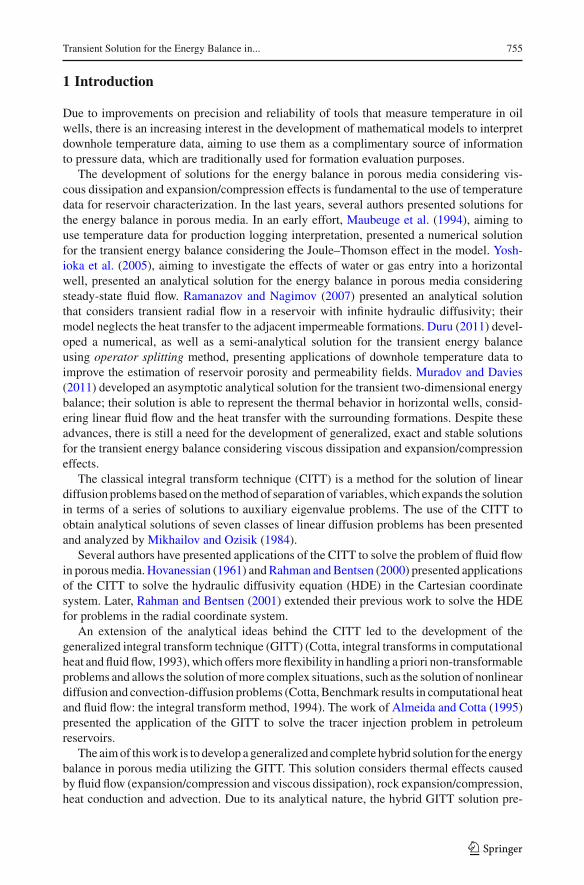
1 Introduction

Due to improvements on precision and reliability of tools that measure temperature in oilwells, there is an increasing interest in the development of mathematical models to interpretdownhole temperature data, aiming to use them as a complimentary source of informationto pressure data, which are traditionally used for formation evaluation purposes.

The development of solutions for the energy balance in porous media considering vis-cous dissipation and expansion/compression effects is fundamental to the use of temperaturedata for reservoir characterization. In the last years, several authors presented solutions forthe energy balance in porous media. In an early effort, Maubeuge et al. (1994), aiming touse temperature data for production logging interpretation, presented a numerical solutionfor the transient energy balance considering the Joule–Thomson effect in the model. Yosh-ioka et al. (2005), aiming to investigate the effects of water or gas entry into a horizontalwell, presented an analytical solution for the energy balance in porous media consideringsteady-state fluid flow. Ramanazov and Nagimov (2007) presented an analytical solutionthat considers transient radial flow in a reservoir with infinite hydraulic diffusivity; theirmodel neglects the heat transfer to the adjacent impermeable formations. Duru (2011) devel-oped a numerical, as well as a semi-analytical solution for the transient energy balanceusing operator splitting method, presenting applications of downhole temperature data toimprove the estimation of reservoir porosity and permeability fields. Muradov and Davies(2011) developed an asymptotic analytical solution for the transient two-dimensional energybalance; their solution is able to represent the thermal behavior in horizontal wells, consid-ering linear fluid flow and the heat transfer with the surrounding formations. Despite theseadvances, there is still a need for the development of generalized, exact and stable solutionsfor the transient energy balance considering viscous dissipation and expansion/compressioneffects.

The classical integral transform technique (CITT) is a method for the solution of lineardiffusion problems based on themethod of separation of variables,which expands the solutionin terms of a series of solutions to auxiliary eigenvalue problems. The use of the CITT toobtain analytical solutions of seven classes of linear diffusion problems has been presentedand analyzed by Mikhailov and Ozisik (1984).

Several authors have presented applications of the CITT to solve the problem of fluid flowin porousmedia. Hovanessian (1961) andRahman andBentsen (2000) presented applicationsof the CITT to solve the hydraulic diffusivity equation (HDE) in the Cartesian coordinatesystem. Later, Rahman and Bentsen (2001) extended their previous work to solve the HDEfor problems in the radial coordinate system.

An extension of the analytical ideas behind the CITT led to the development of thegeneralized integral transform technique (GITT) (Cotta, integral transforms in computationalheat and fluid flow, 1993), which offersmore flexibility in handling a priori non-transformableproblems and allows the solution ofmore complex situations, such as the solution of nonlineardiffusion and convection-diffusion problems (Cotta, Benchmark results in computational heatand fluid flow: the integral transform method, 1994). The work of Almeida and Cotta (1995)presented the application of the GITT to solve the tracer injection problem in petroleumreservoirs.

The aimof thiswork is to develop a generalized and complete hybrid solution for the energybalance in porous media utilizing the GITT. This solution considers thermal effects causedby fluid flow (expansion/compression and viscous dissipation), rock expansion/compression,heat conduction and advection. Due to its analytical nature, the hybrid GITT solution pre-

123


sented retains important features of analytical solutions that differentiate them from purelynumerical schemes: (a) stability; (b) controlled accuracy; (c) can be used to provide trendsand asymptotic behaviors, without requiring a complete numerical solution; (d) can providebenchmark results for the validation of numerical schemes applicable to more involved sit-uations; and (e) are more amenable to mathematical treatments for inverse problems andparameters estimation.

2 Problem Formulation

Figure 1 presents an illustrative scheme of the problem to be solved in this work, describ-ing the heat transfer mechanisms as well as the source terms affecting the transient thermalbehavior. Fig. 1 represents an advection-diffusion problem with source terms related to vis-cous dissipation and expansion/compression of rock and fluid. These source terms are relatedto changes in pressure that occur inside the reservoir, in such a way that, to solve the energybalance, it is necessary to solve the hydraulic diffusivity equation, which describes the tran-sient and spatial pressure variations that take place inside a producing reservoir. The HDEneglecting gravitational effects and considering the flow of liquids of low and constant com-pressibility with a source term representing the well production (Wp) can be expressed bythe following formulation (Deucher et al. 2016):

φ(x)ct∂p(x, t)

∂t= ∇.

(k(x)μ

∇ p(x, t))

+ Wp(x, t), x ∈ V, t > 0 (1a)

with generalized boundary conditions:

c(x)p(x, t) + d(x)k(x)μ

∂p(x, t)∂n

= ξ(x, t), x ∈ S, t > 0 (1b)

and generalized initial condition:

p(x, t) = Υ (x), x ∈ V, t = 0 (1c)

wellbore

Heat conduction to the surrounding rocks

Fluid flow towards thewellbore

AdvectionConduction

Source terms related tofluid flow and rock

expansion/compression

Surrounding rocks

Reservoir

Heat conduction to the surrounding rocks

Fig. 1 Illustrative scheme of the problem to be solved in this work

123


where ct represents the total compressibility of the reservoir, accounting for the rock (cr )and fluids present at the pore space compressibilities (oil and water).

Deucher et al. (2016) presented a generalized solution for problem (1) that is going to beconsidered throughout the applications presented in this work. A detailed explanation anddemonstration of this solution, which is based on eigenfunction expansions, can be found inDeucher et al. (2016). It is important to mention that the solution of the energy balance thatis presented does not require the use of the generalized solution of the HDE presented byDeucher et al. (2016), being it possible to use any other solutions of the HDE found in theliterature, such as the ones presented by Carslaw and Jaeger (1959).

The energy balance, as derived by Sui et al. (2008), is given by:

ρCp∂T (x, t)

∂t+ ρ f Cp f ν(x, t).∇T (x, t)

= φ(x)βT (x, t)∂p(x, t)

∂t+ (

p(x, t) + ρrCpr T (x, t))φcr

∂p(x, t)∂t

+ (βT (x, t) − 1) ν(x, t).∇ p(x, t) + ∇. (kT (x)∇T (x, t)) ,

x ∈ V, t > 0. (2)

As observed by Muradov and Davies (2011), in transient temperature analysis, the tempera-ture variations are generally small (∼ 2K) when compared to the initial reservoir temperature(T0 ∼ 350K), making it possible to consider, without significant loss of accuracy, thatφ(x)βT (x, t) ∼= φ(x)βT0, ρrCpr T (x, t) ∼= ρrCpr T0 and (βT (x, t) − 1) ∼= (βT0 − 1),allowing one to linearize Eq. 2:

ρCp∂T (x, t)

∂t+ ρ f Cp f ν(x, t).∇T (x, t)

= φ(x)βT0∂p(x, t)

∂t+ (p(x, t) + ρrCpr T0)φcr

∂p(x, t)∂t

+(βT0 − 1)ν(x, t).∇ p(x, t) + ∇.(kT (x)∇T (x, t)),

x ∈ V, t > 0 (3a)

with generalized boundary conditions:

a(x)T (x, t) + b(x)kT (x)∂T (x, t)

∂n= ϕ(x, t), x ∈ S, t > 0 (3b)

and generalized initial condition:

T (x, t) = f (x), x ∈ V, t = 0 (3c)

the velocity, ν(x, t), is given by Darcy’s Law:

ν(x, t) = −k(x)μ

∇ p(x, t) (4)

Equation (3a) states that the variations of temperature (1st term on the left-hand side) areruled by a series of energy transport and heat release phenomena:

(a) advection (2nd term on the left-hand side);(b) transient expansion/compression of the fluid (1st term on the right-hand side);(c) transient expansion/compression of the rock (2nd term on the right-hand side);(d) spatial expansion/compression of the fluid and viscous dissipation (3rd term on the right-

hand side). This term, in spite of being directly related to the Joule-Thomson coefficient

123


of the fluid, which is given by μJT = (βT0 − 1)/ρ f Cp f , is not the manifestation of theJoule–Thomson effect itself;

(e) heat conduction (4th term on the right-hand side).

3 Formal Solution

The solution of the energy balance given by Eq. (3a–c) can be obtained by the GITT. Accord-ing to Cotta (1993), the basic steps involved in the application of the GITT are: (a) choiceof an appropriate eigenvalue problem; (b) development of the integral transform pair; (c)attempt to integral transform the original partial differential equation; (d) truncate the infi-nite system of coupled ordinary differential equation and solve it to obtain the transformedpotentials; and (e) use the inverse formula to obtain the original potential.

The basic steps presented above are applied to the problem given by Eq. (3a–c) in orderto obtain a generalized and formal solution which can be applied to the interpretation oftransient downhole temperature data.

By applying separation of variables to the homogeneous version of Eq. (3a–c) without theadvective term, the following auxiliary problem is obtained:

∇.(kT (x)∇ψi (x)) + ρCpσ2i ψi (x) = 0, x ε V (5a)

with homogeneous boundary conditions given by:

a(x)ψi (x) + b(x)kT (x)∂ψi (x)

∂n= 0, x ∈ S (5b)

where ψi (x) and σi are the eigenfunctions and eigenvalues of the auxiliary problem, respec-tively. The norms of the auxiliary eigenvalue problem are given by Ni = ∫V ρCpψ

2i (x)dV .

The appropriate inverse-transform pair is obtained at the onset of the problem and is givenby:

Ti (t) = ρCp

∫V

ψi (x)T (x, t)dV (6a)

T (x, t) =∞∑i=1

ψi (x)Ti (t) (6b)

where ψi (x) is the normalized eigenfunction, given by ψi (x) = ψi (x)/N1/2i . Operating Eq.

(3a) with ∫V ψi (x)dV , one obtains:

dTi (t)

dt+ ρ f Cp f

∫V

ψi (x)[ν(x, t).∇T(x,t)

]dV = −σ 2

i Ti (t) + gi (t), t > 0,

i = 1, 2, . . . (7)

the integration of Eq. (7) can be done by substituting the inversion formula Eq. (6b) intoEq. (7):

dTi (t)

dt+ σ 2

i Ti (t) +∞∑j=1

A∗i j (t)T j (t) = gi (t), i = 1, 2, . . . (8a)

123


where

A∗i j (t) = ρ f Cp f

∫V

ψi (x)[ν(x, t).∇ψ j (x)

]dV (8b)

and:

gi (t) =∫V

φβT0∂p(x, t)

∂tψi (x)dV +

∫V

(φcr

(p(x, t) + ρrCpr T0

)) ∂p(x, t)∂t

ψi (x)dV

+∫V

(βT0 − 1) ν(x, t).∇ p(x,t)ψi (x)dV +∫S

ϕ(x, t)[ψi (x) − kT (x) ∂ψi (x)

∂n

]a(x) + b(x)

dS

(8c)

the transformed initial condition is:

Ti (t = 0) = fi = ρCp

∫V

ψi (x) f (x)dV, i = 1, 2 . . . (8d)

If analytical representation of the integrals involved in Eq. (8b–d) are not available, it willbe necessary to numerically integrate these terms. This task, which was not necessary forthe applications presented in this paper, can be performed by consolidated routines withcontrolled accuracy, such as the Gaussian quadrature.

Equation (8a–d) form an infinite system of coupled ordinary differential equations for thetransformed potentials. Computationally, the system of equations is truncated at the N th rowand column, with N large enough to obtain the desired precision. In this work, the system ofcoupled ordinary differential equations is solved using the NDSolve routine ofMathematicaWolfram (2005). Other well established routines in packages of scientific computation, suchas the IMSL Library, available in programming languages such as Fortran and Java could beused. After obtaining the transformed potentials, the inverse formula (Eq. 6b) can be used toobtain the desired potentials.

The formal solution presented in this section is a generalized and complete solution ofthe problem given by Eq. (3a–c) that can be applied to multi-dimensional problems in anyorthogonal coordinate systems, with generalized boundary conditions that can be of the first,second and third kind. The initial condition can be chosen in order to represent the geothermalgradient or any other temperature distribution considered adequate to the problem beinganalyzed, as will be shown in the following applications.

4 Applications

Applications of the formal solution in the Cartesian coordinate system are now going tobe presented. The applications consider a homogeneous reservoir, with constant porosity,permeability and rock thermal properties. It is important to note that the formal solutionpresented in “Formal Solution” section allows the incorporation of variations in rock thermalproperties as well as permoporosities, by following the ideas presented in previous works(Naveira-Cotta et al. 2009; Deucher et al. 2016).

Figure 2 represents an illustration of the problem to be solved, with its boundary conditionsand characteristic dimensions.

123


zx

xp

Lx

Lz

Ladj

Ladj

Ltot

Surrounding rocks

Reservoir

Fig. 2 Illustrative scheme of the applications

The problem in Fig. 2 consists of a two-dimensional heat transfer problem, where fluidflows toward a long horizontal well (placed at the position xp) in a thin reservoir.

The modeling of the horizontal well as a plane sink assumes that:

(a) the streamlines can all be treated as linear in the reservoir and parallel to the x-axis. Thisis a common assumption in pressure transient analysis that is also applied to the transienttemperature problem;

(b) the temperature, pressure and flow velocity fields are uniformly distributed in they-direction, allowing the exclusion of the y-dimension from the analysis. This approxi-mation holds if thewell length is equal to the reservoir dimension parallel to thewellbore.

These assumptions were already used byMuradov and Davies (2011) to present analyticalsolutions for temperature interpretation in horizontal wells. It is important to keep in mindthat these assumptions imply that the early-time radial and late-time radial flow regimes arenot modeled in the following applications.

The modeling of the horizontal well as a plane sink also implies that convective and con-ductive heat transfer between the wellbore and the formation does not occur, as mentionedby App (2010), meaning that the sandface temperature is not affected by the flow inside thewellbore, i.e., the solution represents the pure reservoir response. If necessary, wellbore mod-eling techniques can describe the wellbore flowing temperature provided the pure reservoirresponse is known (Muradov and Davies 2008).

In order to validate the GITT solution, the results are going to be compared with the onesobtained with the asymptotic analytical solution presented by Muradov and Davies (2011)that will be considered as a reference solution. Aiming to preserve the conditions underwhich the reference solution is valid, the same reservoir parameters presented by Muradovand Davies (2011) are considered, as given in Table 1.

It is important to note that the rock compressibility in Table 1 is considered null due tothe fact that the solution presented by Muradov and Davies (2011) did not consider the rockexpansion/compression effects (2nd term on the right-hand side of Eq. 3a). This limitationis overcome by the GITT solution and the impacts of rock expansion/compression on thetransient temperature behavior will be shown in “Two-dimensional Solution” section.

123


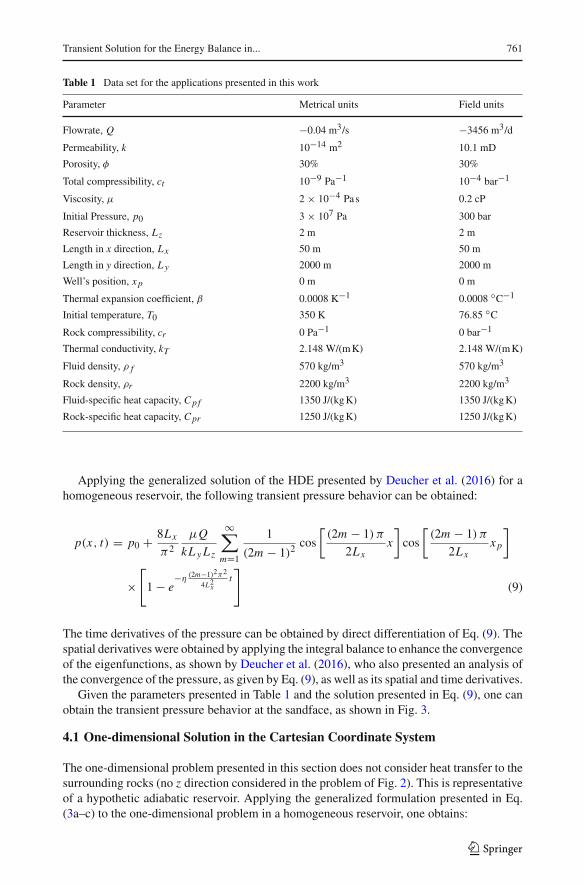
Table 1 Data set for the applications presented in this work

Parameter Metrical units Field units

Flowrate, Q −0.04 m3/s −3456 m3/d

Permeability, k 10−14 m2 10.1 mD

Porosity, φ 30% 30%

Total compressibility, ct 10−9 Pa−1 10−4 bar−1

Viscosity, μ 2 × 10−4 Pa s 0.2 cP

Initial Pressure, p0 3 × 107 Pa 300 bar

Reservoir thickness, Lz 2 m 2 m

Length in x direction, Lx 50 m 50 m

Length in y direction, Ly 2000 m 2000 m

Well’s position, xp 0 m 0 m

Thermal expansion coefficient, β 0.0008 K−1 0.0008 ◦C−1

Initial temperature, T0 350 K 76.85 ◦CRock compressibility, cr 0 Pa−1 0 bar−1

Thermal conductivity, kT 2.148 W/(mK) 2.148 W/(mK)

Fluid density, ρ f 570 kg/m3 570 kg/m3

Rock density, ρr 2200 kg/m3 2200 kg/m3

Fluid-specific heat capacity, Cpf 1350 J/(kgK) 1350 J/(kgK)

Rock-specific heat capacity, Cpr 1250 J/(kgK) 1250 J/(kgK)

Applying the generalized solution of the HDE presented by Deucher et al. (2016) for ahomogeneous reservoir, the following transient pressure behavior can be obtained:

p(x, t) = p0 + 8Lx

π2

μQ

kLyLz

∞∑m=1

1

(2m − 1)2cos

[(2m − 1) π

2Lxx

]cos

[(2m − 1) π

2Lxxp

]

×[1 − e

−η(2m−1)2π2

4L2xt]

(9)

The time derivatives of the pressure can be obtained by direct differentiation of Eq. (9). Thespatial derivatives were obtained by applying the integral balance to enhance the convergenceof the eigenfunctions, as shown by Deucher et al. (2016), who also presented an analysis ofthe convergence of the pressure, as given by Eq. (9), as well as its spatial and time derivatives.

Given the parameters presented in Table 1 and the solution presented in Eq. (9), one canobtain the transient pressure behavior at the sandface, as shown in Fig. 3.

4.1 One-dimensional Solution in the Cartesian Coordinate System

The one-dimensional problem presented in this section does not consider heat transfer to thesurrounding rocks (no z direction considered in the problem of Fig. 2). This is representativeof a hypothetic adiabatic reservoir. Applying the generalized formulation presented in Eq.(3a–c) to the one-dimensional problem in a homogeneous reservoir, one obtains:

123


180

200

220

240

260

280

300

0.0001 0.001 0.01 0.1 1

Pre

ssur

e, b

ar

Time, days

Fig. 3 Transient pressure behavior at the sandface (x = xp)

Table 2 Convergence behavior of sandface temperature for different times

Time, days �T,◦ CNumber of terms (N)

10 25 50 100 150 200

0.1 −0.29519 −0.29959 −0.30106 −0.30174 −0.30177 −0.30178

0.2 −0.34680 −0.35096 −0.35246 −0.35307 −0.35311 −0.35312

0.5 −0.34706 −0.35041 −0.35212 −0.35254 −0.35259 −0.35260

1 −0.31866 −0.32076 −0.32274 −0.32299 −0.32304 −0.32305

5 −0.08768 −0.08446 −0.08609 −0.08640 −0.08645 −0.08646

10 0.20747 0.21000 0.20913 0.20881 0.20877 0.20875

20 0.80808 0.80066 0.79957 0.79925 0.79921 0.79919

ρCp

kT

∂T (x, t)

∂t+ ρ f Cp f

kTν(x, t).∇T (x, t)

= φβT0kT

∂p(x, t)

∂t+(p(x, t) + ρrCpr T0

)φcr

kT

∂p(x, t)

∂t

+ (βT0 − 1)

kTν(x, t).∇ p(x, t) + ∇2T (x, t),

0 < x < Lx , t < 0 (10a)∂T (x, t)

∂x= 0, x = 0, t > 0 (10b)

T (x, t) = 0, x = Lx , t > 0 (10c)

T (x, t) = 0, 0 < x < Lx , t = 0 (10d)

Themathematicalmanipulations involved in the application of the formal solution to problemgiven by Eq. (10a–d) are presented in Appendix 1.

Table 2 presents the convergence behavior of the sandface temperature (x = xp). Thetemperature sensors usually employed in oilfields have a maximum resolution of 0.001 ◦C,thus, for practical purposes, the convergence of three decimal places is enough to considerthe solution converged.

123


-0.4

-0.2

0

0.2

0.4

0.6

0.8

1

1.2

1.4

1.6

0.001 0.01 0.1 1 10

ΔT,

ºC

Time, days

GITT full solutionGITT without advection

Fig. 4 Temperature variations at the sandface (x = xp) with and without the advective transport term

The analysis of Table 2 shows that convergence of three decimal places is obtained with100 terms in the eigenfunction expansion for all the times analyzed and that 25 terms areenough to obtain the convergence of two decimal places, which is already enough for theanalysis of temperature data collected by sensors of 0.01◦C resolution, such as fiber opticsensors.

The transient sandface (x = xp) temperature considering and neglecting advection ispresented in Fig. 4, converged with 200 terms in the eigenfunction expansion.

As can be observed in Fig. 4, the advective transport term has a small impact on thesandface inflow temperature, at least for the parameters presented inTable 1. The possibility ofneglecting the advective term allows one to uncouple the transformed potentials (A∗

i j (t) = 0),making it possible to solve the transformed potentials analytically (not presented in thiswork) and/or with less computational effort. It is important to remember that the possibilityof neglecting the advective term needs to be investigated case by case in order to avoidmisinterpretations of the solutions.

4.1.1 Impact of Initial Temperature Distribution

Wellbore drilling and completion operations may disturb the original reservoir temperature.According to Kutasov (1999), temperature disturbance is affected by the duration of fluidcirculation and shut-in periods, the circulating fluid temperature, the well radius and thethermal properties of the formations.

Aiming to evaluate the impact of these perturbations on the transient temperature behavior,the one-dimensional problemwill be solved by considering a disturbed formation temperaturein the near wellbore region given by:

T (x, 0) = T1 + (T0 − T1)

e−ω(x−xc), 0 < x < Lx , t = 0 (11)

Considering Eq. (11) and the parameters presented in Table 3, the initial conditions that areevaluated in the following analysis are presented in Fig. 5.

The temperature disturbances presented in Fig. 5 do not aim to represent any specificsituation. Indeed, the precise definition of temperature disturbance for a given wellbore at

123


Table 3 Parameters of Eq. 11 tocalculate different initialconditions

Initial condition (IC) T1 (K) ω(m−1

)xc (m)

IC1 – – –

IC2 −0.2 5 0.2

IC3 −0.4 5 0.5

IC4 −0.5 3 1.0

IC5 −0.5 2 2.0

-0.5

-0.4

-0.3

-0.2

-0.1

0

0.1

0 1 2 3 4 5

ΔT,

ºC

Distance, m

IC1IC2IC3IC4IC5

Fig. 5 Set of initial conditions

a given time is a difficult task because some of the factors affecting this disturbance arenot readily available, such as the circulating fluid temperature, which varies with depth,the time and the circulating flowrate. In addition to that, the occurrence of fluid losses tohigh permeability layers poses even more obstacles in obtaining estimates of temperaturedisturbances in the near wellbore region. Thus, the initial conditions presented in Fig. 5 aimto represent uncertain and small temperature perturbations that could influence temperaturetransient analysis, especially during the first start up period of a well.

Solving the energy balance with the initial conditions represented by Eq. (11) with theparameters in Table 3, one obtains the impact of different initial conditions on the transientsandface (x = xp) temperature. The results presented in Fig. 6 are converged with 200 termsin the eigenfunction expansions.

Analyzing the results in Fig. 6, one can notice that small perturbations in the initialtemperature (Fig. 5) have a significant effect on the transient thermal response, especiallybetween 0.1 and 10 days, where both the values of the temperature and the shape of thecurve (related to temperature derivatives) are affected by the initially disturbed temperature.For long times, the effects of the initial condition on the sandface temperature are verysmall, reducing to zero for sufficiently long times. The results presented in Fig. 6 show thatperturbations of the initial reservoir temperature, if not adequately considered, could leadto errors in the interpretation of transient temperature data collected during the first start upperiod of a well, showing the importance of a proper cleanup of the well before transienttemperature data interpretation. In addition to that, the analysis of transient temperature data

123


-1-0.9-0.8-0.7-0.6-0.5-0.4-0.3-0.2-0.1

00.10.20.30.40.50.60.70.80.9

1

0.001 0.01 0.1 1 10

ΔT,

ºC

Time, days

IC1IC2IC3IC4IC5

Fig. 6 Temperature variations at the sandface (x = xp) with different initial conditions

-0.8

-0.7

-0.6

-0.5

-0.4

-0.3

-0.2

-0.1

0

0.1

0.2

0.3

0.4

0 1 2 3 4 5 6 7 8 9 10

ΔT,

ºC

Time, days

IC3 full solutionIC3 without advection

Fig. 7 Temperature variations at the sandface (x = xp) for IC3 with and without advection

can provide information of whether the near wellbore region is fully clean or not, as alreadymentioned by Theuveny et al. (2013).

The advective term, which represented a minor effect in the temperature calculationspresented in Fig. 4, which considers uniform initial temperatures, has an important effectwhen the initial temperature distribution is not uniform. This can be observed in Fig. 7,which shows the transient sandface temperature with initial condition 3 (IC3) of Table 3,considering and neglecting the advective term.

It is important to remember that the results presented in this section did not consider thevariations in the thermal properties of the fluids in the near wellbore region that are causedby drilling fluid invasion. However, even with this simplification, it is possible to concludethat minor temperature perturbations in the near wellbore region, which are generally presentin the first start up period of a well, can have a significant impact on the transient thermalbehavior and consequently on the interpretation of transient temperature data for reservoircharacterization.

123


4.2 Two-dimensional Solution

The two-dimensional problem presented in this section considers the heat transfer to the sur-rounding rocks, as depicted in Figs. 1 and 2. Applying the generalized formulation presentedin Eq. (3a–c) to the two-dimensional problem in a homogeneous reservoir, one obtains:

ρCp

kT

∂T (x, z, t)

∂t+ ρ f Cp f

kTν (x, z, t) · ∇T (x, z, t)

= φβT0kT

∂p (x, z, t)

∂t+(p (x, z, t) + ρrCpr T0

)φcr

kT

∂p (x, z, t)

∂t

+ (βT0 − 1)

kTν (x, z, t) .∇ p (x, z, t) + ∇2T (x, z, t) , 0 < x < Lx ,

0 < z < L tot, t > 0 (12a)∂T (x, z, t)

∂x= 0, x = 0, t > 0 (12b)

T (x, z, t) = 0, x = Lx , t > 0 (12c)

T (x, z, t) = 0, z = 0, t > 0 (12d)

T (x, z, t) = 0, z = L tot, t > 0 (12e)

T (x, z, t) = 0, 0 < x < Lx , 0 < z < L tot, t = 0 (12f)

where

p (x, z, t) ={p(x, t), Ladj < z < Lz + Ladj

0, z ≤ Ladj and z ≥ Lz + Ladj(13)

and the velocity vector, despite of being dependent of the z-direction, is not null only in thex-component, and is given by:

ν (x, z, t) ={

ν(x, t), Ladj < z < Lz + Ladj

0, z ≤ Ladj and z ≥ Lz + Ladj(14)

It is important to mention that the initial condition (Eq. 12f) does not consider thegeothermal heat flow, as this heat flow does not affect the results, according to the superpo-sition principle, as already mentioned by Muradov (2010). The mathematical manipulationsinvolved in the application of the formal solution to the problem given by Eq. (12a–f) arepresented in Appendix 2.

Applying the same parameters presented in Table 1 and considering Ladj = 9m, which islong enough to guarantee the validity of boundary conditions 12d–e throughout thewhole timedomain for which the solution is desired (Deucher 2014), one obtains the results presentedin Table 4, which represent the sandface temperature (x = xp) in a vertical (z) positionequivalent to the center of the reservoir. These results were obtained neglecting the advectiveterm, due to its small impact on the solution, as shown in Fig. 4.

The analysis of Table 4 shows that 150 terms in each direction are sufficient to obtainthe convergence of three decimal places. The computational time to solve the system ofordinary differential equations given by Eqs. (35–38) with 200 terms in each direction is

123


Table 4 Convergence behavior of sandface temperature in the two-dimensional problem

Time, days �T,◦CNumber of terms in each direction (N)

10 25 50 100 150 200

0.1 −0.25698 −0.33065 −0.29779 −0.30517 −0.30195 −0.30153

0.2 −0.30016 −0.38438 −0.34858 −0.35389 −0.35291 −0.35281

0.5 −0.29580 −0.37466 −0.35147 −0.35299 −0.35305 −0.35306

1 −0.26362 −0.32592 −0.31995 −0.31969 −0.31976 −0.31976

5 −0.04113 −0.01885 −0.02628 −0.02556 −0.02562 −0.02563

10 0.17250 0.22470 0.21687 0.21760 0.21754 0.21753

20 0.48541 0.55046 0.54246 0.54319 0.54313 0.54312

40 0.91795 0.98859 0.98058 0.98130 0.98124 0.98123

-0.6-0.4-0.2

00.20.40.60.8

11.21.41.61.8

2

0.001 0.01 0.1 1 10 100

ΔT,

ºC

Time, days

GITTReference solution

Fig. 8 Temperature variations at the wellbore (x = xp) given by the GITT and reference solution

3953 seconds, using an Intel� CoreTM i7-2960XM processor with 32MB RAM memoryinstalled.Althoughnot presented in thiswork, the convergenceof the eigenfunction expansionfor the two-dimensional problem can be accelerated, by properly reordering the terms in theeigenfunction expansions, as presented by Mikhailov and Cotta (1996).

Figure 8 shows the sandface temperature as obtained by the GITT with 200 terms in eachdirection of the eigenfunction expansion, as well as the results obtained by the asymptoticanalytical solution presented by Muradov and Davies (2011), that is here considered as areference solution for purposes of validation.

The analysis of Fig. 8 shows that the GITT and reference solutions are in good agreement.The deviations found between 0.1 and 0.2 days can be explained by the viscous dissipationeffect that is not considered in the reference solution for short times. The reference solutionis presented only for t < 40 days, as it is not valid for longer times. The results presented inFig. 8 validate the solution of the energy balance by the GITT presented in this work.

The GITT solution validated in Fig. 8 is obtained at a higher computational cost than thereference solution, but it brings important advances when compared to previous solutions:

123


(a) It rigorously solves the energy balance using a single formulation valid for the wholespace and time domains;

(b) It is continuous and differentiable;(c) The association of the generalized solution of the energy balance with the generalized

solution of the HDE presented by Deucher et al. (2016) allows one to solve the energybalance for the whole time domain, since the pressure solution considers all flow regimes(transient, late-transient and steady-state/pseudo-steady-state) in a single formulation;

(d) It is general and applicable to problems with variable flowrates and/or different boundaryconditions, allowing, for example, to obtain the solution for bounded-reservoirs, wherea steady-state flow behavior would not be achieved. These applications were not shownin this paper but can be found in Deucher (2014);

(e) It allows the consideration of several producing and thermally interacting layers, as shownahead;

(f) It incorporates the effects of rock compressibility (2nd term on the right-hand side of Eq.3a), as discussed next.

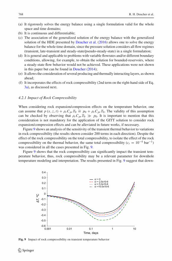
4.2.1 Impact of Rock Compressibility

When considering rock expansion/compression effects on the temperature behavior, onecan assume that p (x, z, t) + ρrCpr T0 ∼= p0 + ρrCpr T0. The validity of this assumptioncan be checked by observing that ρrCpr T0 � p0. It is important to mention that thisconsideration is not mandatory for the application of the GITT solution to consider rockexpansion/compression effects and can be alleviated in future works, if necessary.

Figure 9 shows an analysis of the sensitivity of the transient thermal behavior to variationsin rock compressibility (the results shown consider 200 terms in each direction). Despite theeffect of the rock compressibility on the total compressibility, to isolate the effect of the rockcompressibility on the thermal behavior, the same total compressibility (ct = 10−4 bar−1)

was considered in all the cases presented in Fig. 9.Figure 9 shows that the rock compressibility can significantly impact the transient tem-

perature behavior, thus, rock compressibility may be a relevant parameter for downholetemperature modeling and interpretation. The results presented in Fig. 9 suggest that down-

-0.6

-0.5

-0.4

-0.3

-0.2

-0.1

0

0.1

0.2

0.3

0.4

0.001 0.01 0.1 1 10

ΔT,

ºC

Time, days

cr = 0cr = 2.5x10-6cr = 5.0x10-6cr =10.0x10-6

Fig. 9 Impact of rock compressibility on transient temperature behavior

123


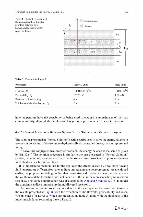
Fig. 10 Illustrative scheme ofthe conjugated heat transferproblem between twohydraulically disconnectedreservoir layers z

x

xp

Lz1

Ladj

Ladj

Lx

Layer 1

Layer 2 Lz2

Lb

Surrounding rocks

Reservoir

Ltot

Table 5 Data set for Layer 2

Parameter Metrical units Field units

Flowrate, Q2 −0.011574 m3/s −1000 m3/d

Permeability, k2 10−15 m2 1.01 mD

Reservoir thickness, Lz2 4 m 4 m

Thickness of the flow barrier, Lb 2 m 2 m

hole temperature have the possibility of being used to obtain in-situ estimates of the rockcompressibility, although this application has yet to be proven in field data interpretation.

4.2.2 Thermal Interaction Between Hydraulically Disconnected Reservoir Layers

The solution presented in “Formal Solution” section can be used to solve the energy balance ina reservoir consisting of two (or more) hydraulically disconnected layers, such as representedin Fig. 10.

To solve this conjugated heat transfer problem, the energy balance is the same as givenby Eq. 12a–f. The solution procedure is similar to the one presented in “Formal Solution”section, being it only necessary to calculate the source terms associated to pressure changesindividually in each reservoir layer.

It is important to mention that for the top layer, the effects caused by a wellbore flowingfluid temperature different from the sandface temperature are not represented. As mentionedearlier, the proposed modeling implies that convective and conductive heat transfer betweenthe wellbore and the formation does not occur, i.e., the solution represents the pure reservoirresponse. This same simplification was also applied by App and Yoshioka (2013) to modelthe transient sandface temperature in multilayered reservoirs.

The flow and reservoir properties considered in this example are the same used to obtainthe results presented in Fig. 8, with the exception of the flowrate, permeability and reser-voir thickness for Layer 2, which are presented in Table 5, along with the thickness of theimpermeable layer separating Layers 1 and 2.

123


100

120

140

160

180

200

220

240

260

280

300

-0.5

-0.4

-0.3

-0.2

-0.1

0

0.1

0.2

0 1 2 3 4 5 6 7 8 9 10

Pre

ssur

e, b

ar

ΔT,

ºC

Time, days

Temperature, Layer 1Temperature, Layer 2Pressure, Layer 1Pressure, Layer 2

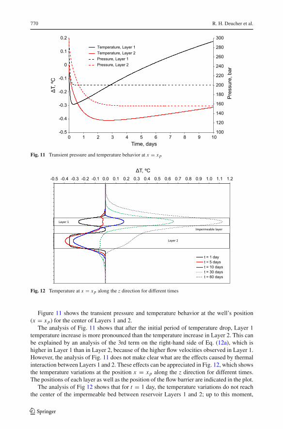
Fig. 11 Transient pressure and temperature behavior at x = xp

-0.5 -0.4 -0.3 -0.2 -0.1 0.0 0.1 0.2 0.3 0.4 0.5 0.6 0.7 0.8 0.9 1.0 1.1 1.2

ΔT, ºC

t = 1 dayt = 5 dayst = 10 dayst = 30 dayst = 60 days

Layer 2

Layer 1

Impermeable layer

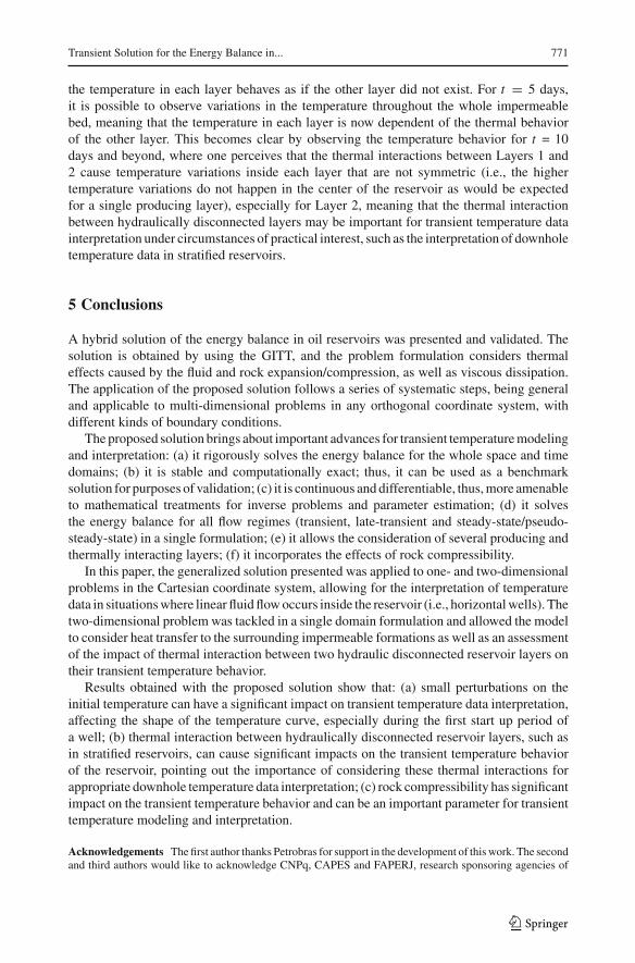
Fig. 12 Temperature at x = xp along the z direction for different times

Figure 11 shows the transient pressure and temperature behavior at the well’s position(x = xp) for the center of Layers 1 and 2.

The analysis of Fig. 11 shows that after the initial period of temperature drop, Layer 1temperature increase is more pronounced than the temperature increase in Layer 2. This canbe explained by an analysis of the 3rd term on the right-hand side of Eq. (12a), which ishigher in Layer 1 than in Layer 2, because of the higher flow velocities observed in Layer 1.However, the analysis of Fig. 11 does not make clear what are the effects caused by thermalinteraction between Layers 1 and 2. These effects can be appreciated in Fig. 12, which showsthe temperature variations at the position x = xp along the z direction for different times.The positions of each layer as well as the position of the flow barrier are indicated in the plot.

The analysis of Fig 12 shows that for t = 1 day, the temperature variations do not reachthe center of the impermeable bed between reservoir Layers 1 and 2; up to this moment,

123


the temperature in each layer behaves as if the other layer did not exist. For t = 5 days,it is possible to observe variations in the temperature throughout the whole impermeablebed, meaning that the temperature in each layer is now dependent of the thermal behaviorof the other layer. This becomes clear by observing the temperature behavior for t = 10days and beyond, where one perceives that the thermal interactions between Layers 1 and2 cause temperature variations inside each layer that are not symmetric (i.e., the highertemperature variations do not happen in the center of the reservoir as would be expectedfor a single producing layer), especially for Layer 2, meaning that the thermal interactionbetween hydraulically disconnected layers may be important for transient temperature datainterpretation under circumstances of practical interest, such as the interpretation of downholetemperature data in stratified reservoirs.

5 Conclusions

A hybrid solution of the energy balance in oil reservoirs was presented and validated. Thesolution is obtained by using the GITT, and the problem formulation considers thermaleffects caused by the fluid and rock expansion/compression, as well as viscous dissipation.The application of the proposed solution follows a series of systematic steps, being generaland applicable to multi-dimensional problems in any orthogonal coordinate system, withdifferent kinds of boundary conditions.

The proposed solution brings about important advances for transient temperaturemodelingand interpretation: (a) it rigorously solves the energy balance for the whole space and timedomains; (b) it is stable and computationally exact; thus, it can be used as a benchmarksolution for purposes of validation; (c) it is continuous and differentiable, thus,more amenableto mathematical treatments for inverse problems and parameter estimation; (d) it solvesthe energy balance for all flow regimes (transient, late-transient and steady-state/pseudo-steady-state) in a single formulation; (e) it allows the consideration of several producing andthermally interacting layers; (f) it incorporates the effects of rock compressibility.

In this paper, the generalized solution presented was applied to one- and two-dimensionalproblems in the Cartesian coordinate system, allowing for the interpretation of temperaturedata in situationswhere linear fluidflowoccurs inside the reservoir (i.e., horizontalwells). Thetwo-dimensional problem was tackled in a single domain formulation and allowed the modelto consider heat transfer to the surrounding impermeable formations as well as an assessmentof the impact of thermal interaction between two hydraulic disconnected reservoir layers ontheir transient temperature behavior.

Results obtained with the proposed solution show that: (a) small perturbations on theinitial temperature can have a significant impact on transient temperature data interpretation,affecting the shape of the temperature curve, especially during the first start up period ofa well; (b) thermal interaction between hydraulically disconnected reservoir layers, such asin stratified reservoirs, can cause significant impacts on the transient temperature behaviorof the reservoir, pointing out the importance of considering these thermal interactions forappropriate downhole temperature data interpretation; (c) rock compressibility has significantimpact on the transient temperature behavior and can be an important parameter for transienttemperature modeling and interpretation.

Acknowledgements The first author thanks Petrobras for support in the development of thiswork. The secondand third authors would like to acknowledge CNPq, CAPES and FAPERJ, research sponsoring agencies of

123


the Brazilian and Rio de Janeiro State governments, for the continuous support of all their research activitiesover the years.

6 Appendix 1

Applying the method of separation of variables to the problem given by Eq. (10a–c), one canobtain the chosen eigenvalue problem:

∂2ψi (x)

∂x2+ ρCp

kTσ 2i ψi (x) = 0, 0 < x < Lx (15)

∂ψi (x)

∂x= 0, at x = 0 (16)

ψi (x) = 0, at x = Lx (17)

consulting the tabulated solutions in the textbook by Ozisik (1993), one can find the eigen-functions, eigenvalues and norms of the eigenvalue problem:

ψi (x) = cos

⎛⎝√

ρCp

kTσi x

⎞⎠ (18)

σi = (2i − 1) π

2Lx

√kT

ρCp(19)

Nx,i = Lx

2

ρCp

kT(20)

using the generalized solution of “Formal Solution” section, the inverse-transform pair canbe written as:

Ti (t) = ρCp

kT

Lx∫0

1

N 1/2x,i

cos

[(2i − 1) π

2Lxx

]T (x, t)dx (21)

T (x, t) =∞∑i=1

1

N 1/2x,i

cos

[(2i − 1) π

2Lxx

]Ti (t) (22)

performing the operations indicated in “Formal Solution” section, one obtains the coupledsystem of ordinary differential equations to be solved in order to obtain the transformedpotentials.

dTi (t)

dt+[

(2i − 1) π

2Lx

√kT

ρCp

]2Ti (t) +

∞∑j=1

A∗im (t) Tm (t) = gi (t) , i = 1, 2, . . .

(23)

where

A∗im (t) = ρ f Cp f

kT N1/2x,i N

1/2x,m

Lx∫0

cos

[(2i − 1) π

2Lxx

]

× d

dx

{cos

[(2m − 1) π

2Lxx

]}(− k

μ

∂p(x, t)

∂x

)dx (24)

123


gi (t) = 1

kT N12x,i

⎧⎨⎩φβT0

Lx∫0

cos

[(2i − 1) π

2Lxx

]∂p(x, t)

∂tdx

+φcr

Lx∫0

(p(x, t) + ρrCpr T0

)cos

[(2i − 1) π

2Lxx

]∂p(x, t)

∂tdx

+ (βT0 − 1)

Lx∫0

cos

[(2i − 1) π

2Lxx

][− k

μ

(∂p(x, t)

∂x

)2]dx

⎫⎬⎭ (25)

The transformed initial condition is given by:

Ti (0) = fi = 0, i = 1, 2 . . . (26)

The calculation of the integrals in Eqs. 24 and 25 was performed using the platformMathe-matica (Wolfram2005), by substituting the expressions for p (x, t) obtained from the solutionof the HDE. It was possible to obtain all the integrals analytically for the cases presentedin this paper, reducing the numerical task associated with the solution without any loss ofaccuracy.

7 Appendix 2

Applying the method of separation of variables to the problem given by Eq. (12a–f), onecan obtain the chosen eigenvalue problems. The eigenvalue problem in the x-direction, aswell as the eigenfunction and eigenvalues are the same given in Appendix 1; the x-direction

norms in the two-dimensional problem are now given by Nx,i = Lx/2(ρCp/kT

)1/2. For

the z-direction, we have:

∂2Ω j (z)

∂z2+ ρCp

kTχ2j Ω j (z) = 0, 0 < z < L tot (27)

Ω j (z) = 0, at z = 0 (28)

Ω j (z) = 0, at z = L tot (29)

Consulting the tabulated solutions in the textbook by Ozisik (1993), one can find the eigen-functions, eigenvalues and norms of the eigenvalue problem in the z-direction:

Ω j (z) = sin

⎛⎝√

ρCp

kTχ j z

⎞⎠ (30)

χ j = jπ

L tot

√kT

ρCp(31)

Nz, j = L tot

2

(ρCp/kT

)1/2(32)

123


Using the generalized solution of “Formal Solution” section, the inverse-transform pair canbe written as:

Ti j (t) = ρCp

kT

Lx∫0

L tot∫0

1

N 1/2x,i N

1/2z, j

cos

[(2i − 1) π

2Lxx

]sin

(jπ

L totz

)T (x, z, t) dxdz (33)

T (x, z, t) =∞∑i=1

∞∑j=1

1

N 1/2x,i N

1/2z, j

cos

[(2i − 1) π

2Lxx

]sin

(jπ

L totz

)Ti j (t) (34)

Performing the operations indicated in “Formal Solution” section, one obtains the coupledsystem of ordinary differential equations to be solved in order to obtain the transformedpotentials.

dTi j (t)

dt+⎧⎨⎩[

(2i − 1) π

2Lx

√kT

ρCp

]2+[

jπ

L tot

√kT

ρCp

]2⎫⎬⎭ Ti j (t)

+∞∑

m=1

∞∑n=1

A∗im jn (t) Tmn (t)

= gi j (t) , i = 1, 2, . . . , j = 1, 2, ... (35)

where

A∗im jn (t) = ρ f Cp f

kT

1

N12x,i N

12z, j N

12x,mN

12z,n

∫ Lx

0

∫ L tot

0cos

[(2i − 1) π

2Lxx

]

× d

dx

{cos

[(2m − 1) π

2Lxx

]}sin

(jπ

L totz

)d

dz

[sin

(nπ

L totz

)]

×(

− k

μ

∂p (x, z, t)

∂x

)dxdz (36)

gi j (t) = 1

kT N1/2x,i N1/2

z, j

{φβT0

∫ Lx

0

∫ L tot

0cos

[(2i − 1) π

2Lxx

]sin

(jπ

L totz

)∂p (x, z, t)

∂tdxdz

+φcr

∫ Lx

0

∫ L tot

0

(p (x, z, t) + ρrCpr T0

)cos

[(2i − 1) π

2Lxx

]sin

(jπ

L totz

)∂p (x, z, t)

∂tdxdz

+ (βT0 − 1)∫ Lx

0

∫ L tot

0cos

[(2i − 1) π

2Lxx

]sin

(jπ

L totz

)[− k

μ

(∂p (x, z, t)

∂x

)2]dxdz

}

(37)

The transformed initial condition is given by:

Ti j (0) = fi j = 0, i = 1, 2 . . . , j = 1, 2 . . . (38)

The solution of the problem given by Eqs. (35–38), which represent a specific case of gen-eralized Eq. (8a–d), was obtained by substituting the expressions for the eigenfunction,eigenvalues and initial conditions into the generalized forms given in Eq. (8a–d). Furtherdetails on the procedure to derive Eq. (35) can be found in Cotta (1993).

The calculationof the integrals in equationsB10andB11wasperformedusing the platformMathematica (Wolfram 2005), by substituting the expressions for p (x, z, t) obtained fromthe solution of the HDE. It was possible to obtain all the integrals analytically for the casespresented in this paper, reducing the numerical task associated with the solution without anyloss of accuracy.

123


References

Almeida, A., Cotta, R.: Integral transformmethodology for convection-diffusion problems in petroleum reser-voir engineering. Int. J. Heat Mass Transf. 38, 3359–3367 (1995)

App, J.F.: Nonisothermal and productivity behavior of high-pressure reservoirs. SPE Journal 15, 50–63 (2010)App, J.F., Yoshioka, K.: Impact of reservoir permeability on flowing sandface temperature: dimensionless

analysis. SPE Journal 18, 685–694 (2013)Carslaw, H., Jaeger, J.: Conduction of Heat in Solids. Clarendon Press, Oxford (1959)Cotta, R.: Integral Transforms in Computational Heat and Fluid Flow. CRC Press, Boca Raton (1993)Cotta, R.: Benchmark results in computational heat and fluid flow: the integral transform method. Int. J. Heat

Mass Transf. 37, 381–393 (1994)Deucher, R.H.: Solution of the energy balance in petroleum reservoirs by the generalized integral transform

technique (in Portuguese) M.Sc. Thesis. Mechanical Engineering Program/COPPE, Federal Universityof Rio de Janeiro (2014)

Deucher, R.H., Couto, P., Bodstein,G.C.R.: Comprehensive solution for transient flow in heterogeneous porousmedia. Transp. Porous Media. 113(3), 549–566 (2016)

Duru, O.: Reservoir analysis and parameter estimation constrained to pressure, temperature and flowratehistories. Ph.D. Thesis, Dept. of Energy Resources Engineering, Stanford University (2011)

Hovanessian, S.: Pressure studies in bounded reservoirs. SPE J. 1, 223–228 (1961)Kutasov, I.M.: Applied Geothermics for Petroleum Engineers. Elsevier, Amsterdam (1999)Maubeuge, F., Didek, M.P., Deardsell, M.B., Caltagirone, J.P.: Temperature model for flow in porous media

andwellbore. Presented at the SPWLA35thAnnual Logging Symposium, Tulsa, Oklahoma,USA, 19–22June (1994)

Mikhailov, M., Cotta, R.: Ordering rules for double and triple eigenseries in the solution of multidimensionalheat and fluid flow problems. Int Commun. Heat Mass Transf 23, 299–303 (1996)

Mikhailov, M., Ozisik, M.: Unified Analysis and Solutions of Heat and Mass Diffusion. Wiley, New York(1984)

Muradov, K.M.: Temperature modelling and real-time flow rate allocation in wells with advanced completion.Ph.D. Thesis, Institute of Petroleum Engineering, Heriot-Watt University (2010)

Muradov, K.M., Davies, D.R.: Prediction of temperature distribution in intelligent wells. Presented at the SPERussian Oil and Gas Technical Conference and Exhibition, Moscow, Russia, 28–30 October (2008)

Muradov, K.M., Davies, D.R.: Novel analytical methods of temperature interpretation in horizontal wells. SPEJ. 16(03), 637–647 (2011)

Naveira-Cotta, C.P., Cotta, R.M.,Orlande,H.R.B., Fudym,O.: Eigenfunction expansions for transient diffusionin heterogeneous media. Int J Heat Mass Transf 52(21–22), 5029–5039 (2009)

Ozisik, M.: Heat Conduction. Wiley, New York (1993)Rahman, N., Bentsen, R.: Use of an integral transform technique for comprehensive solutions to transient flow

problems in homogeneous domains. s.l., s.n (2000)Rahman, N., Bentsen, R.: Comprehensive Solutions for Transient-Flow Problems in 3D Homogeneous

Domains. s.l., s.n (2001)Ramanazov, A., Nagimov, V.: Analytical model for the calculation of temperature distribution in the oil

reservoir during unsteady fluid flow. Oil Gas Bus. 1 (2007). (http://ogbus.ru/eng/authors/Ramazanov/Ramazanov_2e.pdf)

Sui, W., Zhu, D., Hill, A.D., Ehlig-Economides, C.: Model for transient temperature and pressure behaviorin commingled vertical wells. SPE Paper no. 115200-MS. Presented at the SPE Russian Oil and GasTechnical Conference and Exhibition, Moscow (2008)

Theuveny, B.C.,Mikhailov,D., Spesivtsev, P., Starostin,A., Osiptsov,A.A., Sidorova,M., Shako,V.: Integratedapproach to simulation of near-wellbore and wellbore cleanup. SPE Paper no. 166509-MS. Presented atthe SPE Annual Technical Conference and Exhibition, New Orleans, Lousiana, USA (2013)

Wolfram, S.: The Mathematica Book, Version 5.2. Wolfram Media, Cambridge (2005)Yoshioka, K., Hill, A.D., Dawkrajai, P., Lake, L.W.: A comprehensive model of temperature behavior in

a horizontal well. SPE Paper no. 95656-MS. Presented at the SPE Annual Technical Conference andExhibition, Dallas, Texas, USA, 9–12 October (2005)

123

http://ogbus.ru/eng/authors/Ramazanov/Ramazanov_2e.pdf

http://ogbus.ru/eng/authors/Ramazanov/Ramazanov_2e.pdf

transient solution for the energy balance in porous media

Documents