transformations angel: chapter 3 ppt from angel, aw, harvard and mit open courseware, etc. csci 6360...
TRANSCRIPT
TransformationsAngel: Chapter 3
ppt from Angel, AW, Harvard and MIT Open Courseware, etc.
CSCI 6360
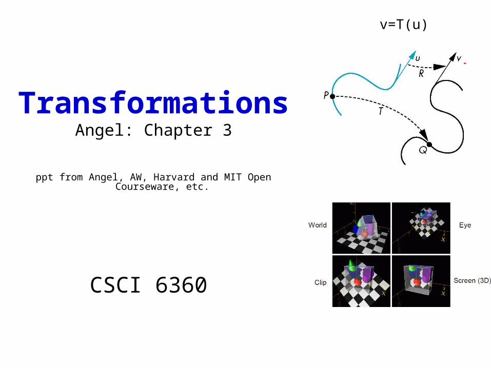
v=T(u)
Overview• Think about “math, transformations, …” in both intuitive/practical-
graphics way and mathematical way
• Transformations– Scaling, translation, rotation– OpenGL state of “viewing” matrix
• Geometry – Elements of geometry: Scalars, Vectors, Points– Introduce concepts such as dimension and basis– Introduce coordinate systems from geometry and cg perspectives
• Used to represent vectors spaces and frames for represent affine spaces• Discuss change of frames and bases• Introduce homogeneous coordinates• Develop mathematical operations among elements in a coordinate-free
manner– Important because of cg implementation
• Show OGL use … probably next time
About
• Relation of mathematic description and computer graphic application
• Presents an explication of coordinate free approach to geometry of interest in cg
– That’s coordinate free – surely not for cg– Purely abstract, the “robust mathematical foundation”– Consider change in frames
• As implementation change in axes orientations
– Consider homogenous coordinates• Mathematic view that leads to efficient implementation
• We’ll look at computer graphics applications first
Recall, Polygon Mesh Representation… now, points through a geometry pipeline
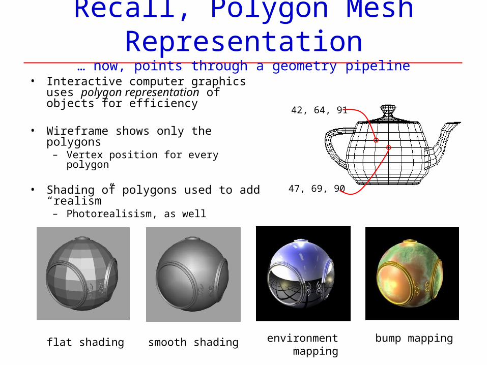
• Interactive computer graphics uses polygon representation of objects for efficiency
• Wireframe shows only the polygons– Vertex position for every polygon
• Shading of polygons used to add “realism”
– Photorealisism, as well
smooth shading environment mapping
bump mappingflat shading
42, 64, 91
47, 69, 90
Polygon Mesh Representation… now, points through a geometry pipeline
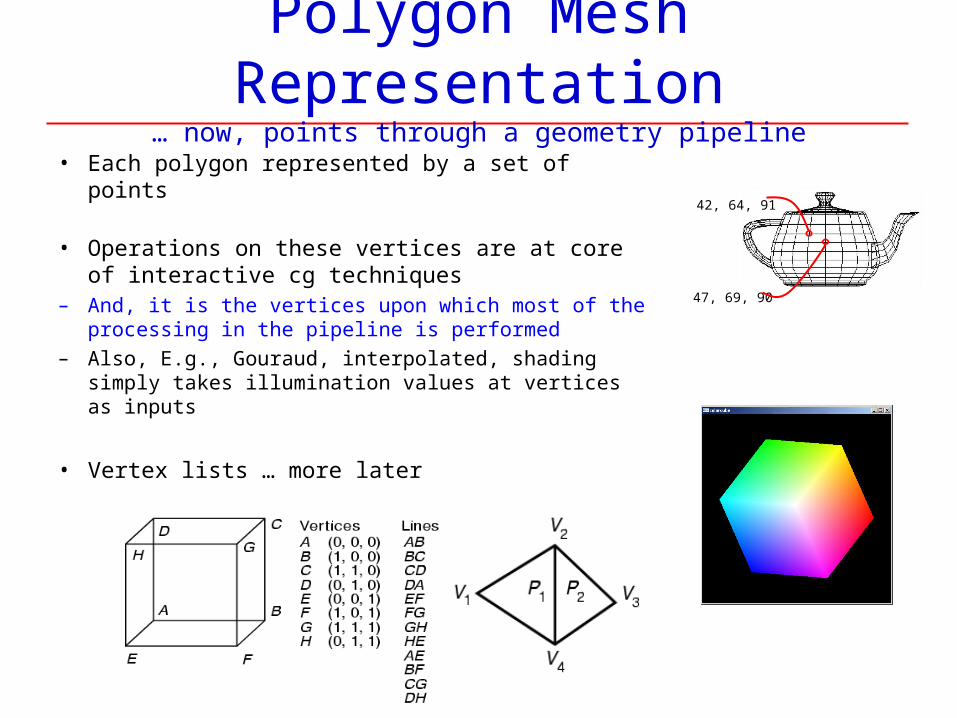
• Each polygon represented by a set of points
• Operations on these vertices are at core of interactive cg techniques
– And, it is the vertices upon which most of the processing in the pipeline is performed
– Also, E.g., Gouraud, interpolated, shading simply takes illumination values at vertices as inputs
• Vertex lists … more later
42, 64, 91
47, 69, 90
Recall, Coordinate Systems in ViewingTransformations of these coordinate systems at core of graphics pipeline!
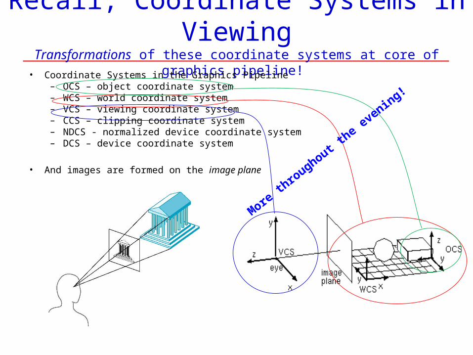
• Coordinate Systems in the Graphics Pipeline – OCS – object coordinate system – WCS – world coordinate system – VCS – viewing coordinate system – CCS – clipping coordinate system – NDCS - normalized device coordinate system – DCS – device coordinate system
• And images are formed on the image plane
More th
roughout t
he evening!
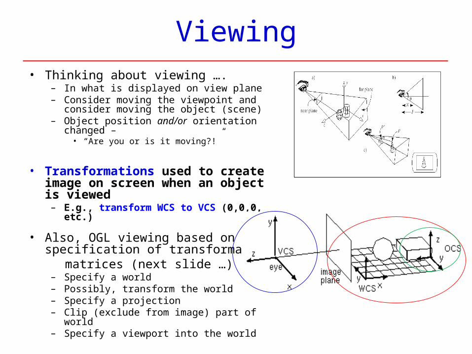
Viewing• Thinking about viewing ….
– In what is displayed on view plane– Consider moving the viewpoint and consider
moving the object (scene)– Object position and/or orientation changed –
• “Are you or is it moving?!”
• Transformations used to create image on screen when an object is viewed
– E.g., transform WCS to VCS (0,0,0, etc.)
• Also, OGL viewing based on specification of transformation
matrices (next slide …)– Specify a world– Possibly, transform the world– Specify a projection– Clip (exclude from image) part of world– Specify a viewport into the world
OpenGLFocus on trans. & matrices
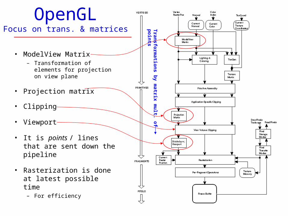
• ModelView Matrix– Transformation of elements
for projection on view plane
• Projection matrix
• Clipping
• Viewport
• It is points / lines that are sent down the pipeline
• Rasterization is done at latest possible time
– For efficiency
Tra
ns
form
atio
ns
by
ma
trix m
ult. o
f po
ints
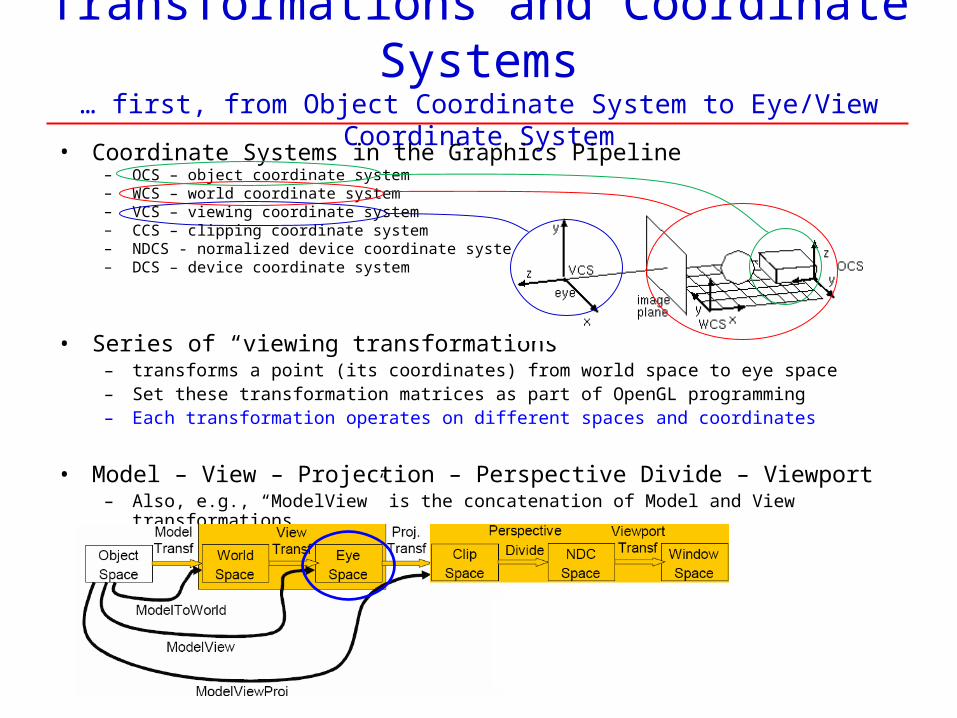
Transformations and Coordinate Systems… first, from Object Coordinate System to Eye/View Coordinate System
• Coordinate Systems in the Graphics Pipeline – OCS – object coordinate system – WCS – world coordinate system – VCS – viewing coordinate system – CCS – clipping coordinate system – NDCS - normalized device coordinate system – DCS – device coordinate system
• Series of “viewing transformations”– transforms a point (its coordinates) from world space to eye space– Set these transformation matrices as part of OpenGL programming– Each transformation operates on different spaces and coordinates
• Model – View – Projection – Perspective Divide – Viewport– Also, e.g., “ModelView” is the concatenation of Model and View transformations
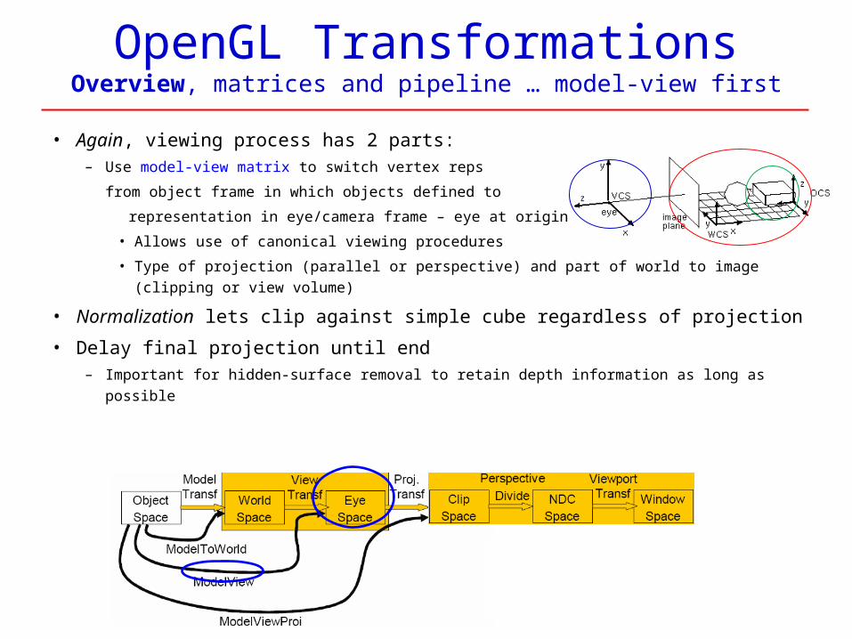
OpenGL TransformationsOverview, matrices and pipeline … model-view first
• Again, viewing process has 2 parts:– Use model-view matrix to switch vertex reps
from object frame in which objects defined to
representation in eye/camera frame – eye at origin
• Allows use of canonical viewing procedures
• Type of projection (parallel or perspective) and part of world to image (clipping or view
volume)
• Normalization lets clip against simple cube regardless of projection
• Delay final projection until end– Important for hidden-surface removal to retain depth information as long as possible
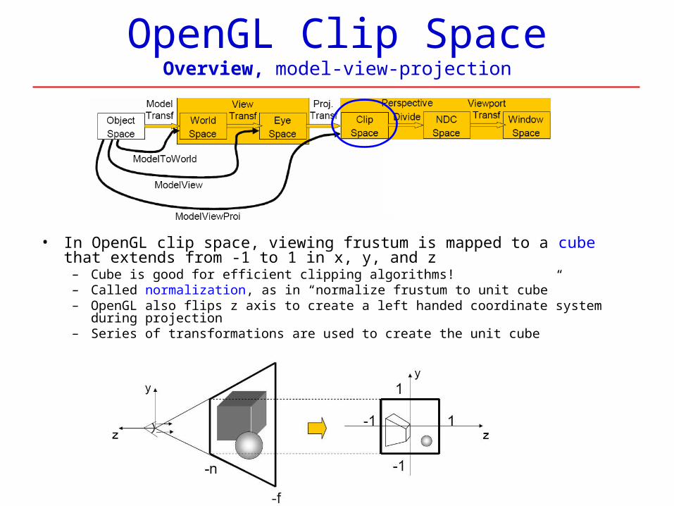
OpenGL Clip SpaceOverview, model-view-projection
• In OpenGL clip space, viewing frustum is mapped to a cube that extends from -1 to 1 in x, y, and z
– Cube is good for efficient clipping algorithms!– Called normalization, as in “normalize frustum to unit cube”– OpenGL also flips z axis to create a left handed coordinate system during projection– Series of transformations are used to create the unit cube
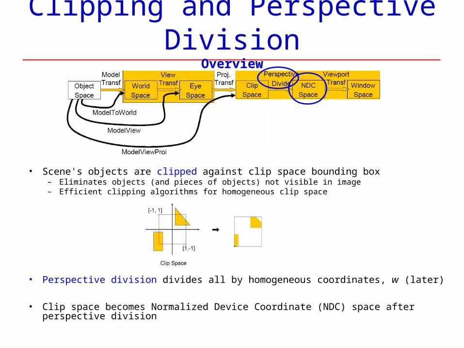
Clipping and Perspective DivisionOverview
• Scene's objects are clipped against clip space bounding box– Eliminates objects (and pieces of objects) not visible in image– Efficient clipping algorithms for homogeneous clip space
• Perspective division divides all by homogeneous coordinates, w (later)
• Clip space becomes Normalized Device Coordinate (NDC) space after perspective division

Viewport TransformationOverview
• OpenGL provides function to set up viewport transformation:
– glViewport(x, y, width, height)– Maps NDC space to window (screen)
space– And we’re done!!!!!!!!!
• Straightforward:– Though need attend to aspect ratio
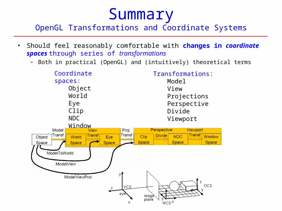
SummaryOpenGL Transformations and Coordinate Systems
• Should feel reasonably comfortable with changes in coordinate spaces through series of transformations
– Both in practical (OpenGL) and (intuitively) theoretical terms
Coordinate spaces:ObjectWorldEyeClipNDCWindow
Transformations:ModelViewProjectionsPerspective DivideViewport
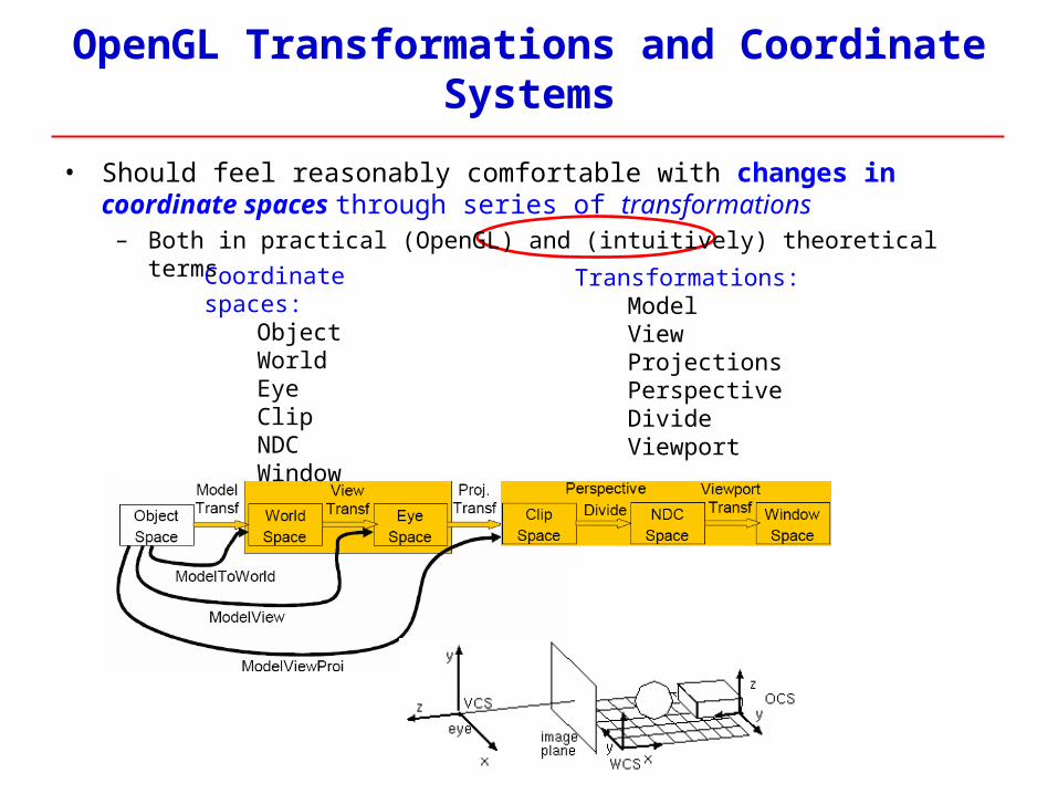
OpenGL Transformations and Coordinate Systems
Coordinate spaces:ObjectWorldEyeClipNDCWindow
Transformations:ModelViewProjectionsPerspective DivideViewport
• Should feel reasonably comfortable with changes in coordinate spaces through series of transformations
– Both in practical (OpenGL) and (intuitively) theoretical terms
Transformations
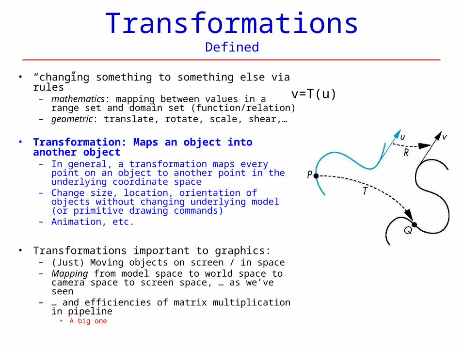
TransformationsDefined
• “changing something to something else via rules”– mathematics: mapping between values in a range
set and domain set (function/relation)– geometric: translate, rotate, scale, shear,…
• Transformation: Maps an object into another object
– In general, a transformation maps every point on an object to another point in the underlying coordinate space
– Change size, location, orientation of objects without changing underlying model (or primitive drawing commands)
– Animation, etc.
• Transformations important to graphics:– (Just) Moving objects on screen / in space– Mapping from model space to world space to
camera space to screen space, … as we’ve seen– … and efficiencies of matrix multiplication in pipeline
• A big one
v=T(u)
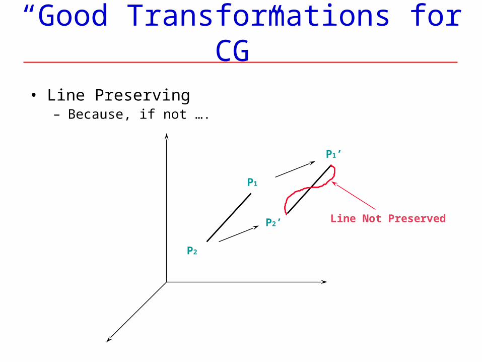
“Good Transformations for CG”
• Line Preserving– Because, if not ….
P1’
P2’
P1
P2
Line Not Preserved
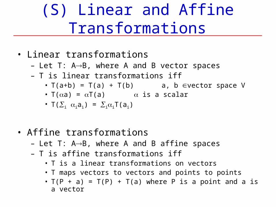
(S) Linear and Affine Transformations
• Linear transformations– Let T: AB, where A and B vector spaces– T is linear transformations iff
• T(a+b) = T(a) + T(b) a, b vector space V• T(a) = T(a) is a scalar• T(i iai) = iiT(ai)
• Affine transformations– Let T: AB, where A and B affine spaces– T is affine transformations iff
• T is a linear transformations on vectors• T maps vectors to vectors and points to points• T(P + a) = T(P) + T(a) where P is a point and a is a vector
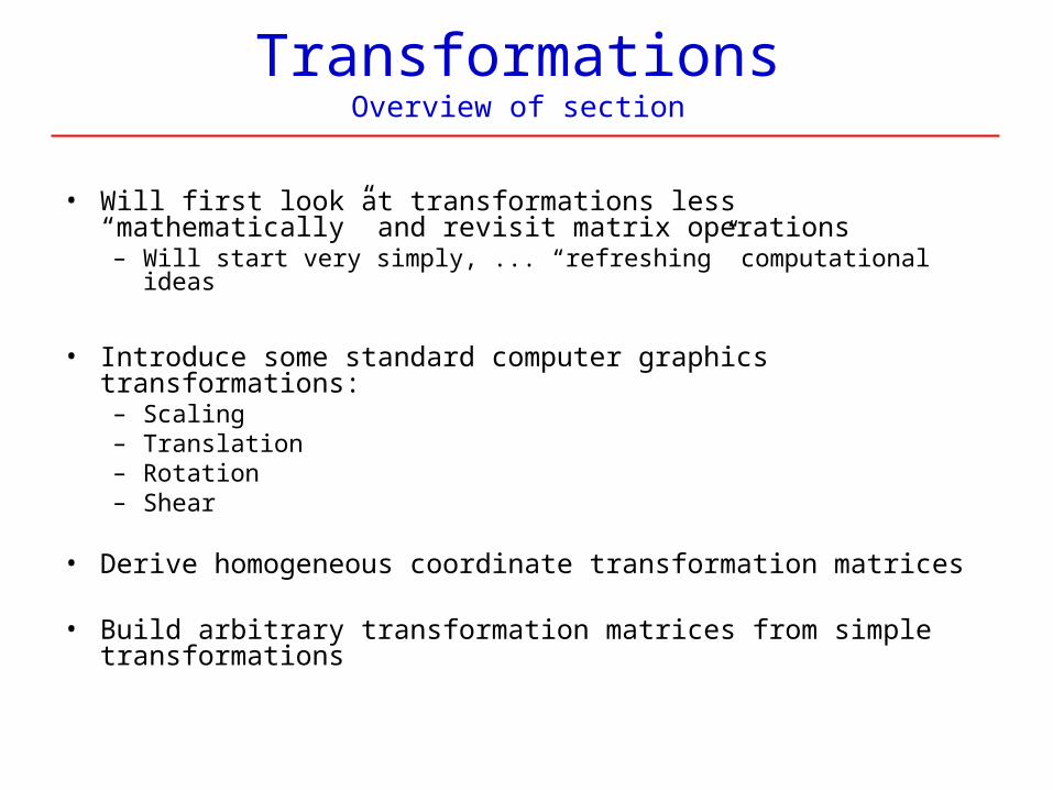
TransformationsOverview of section
• Will first look at transformations less “mathematically” and revisit matrix operations– Will start very simply, ... “refreshing” computational ideas
• Introduce some standard computer graphics transformations:– Scaling– Translation– Rotation– Shear
• Derive homogeneous coordinate transformation matrices
• Build arbitrary transformation matrices from simple transformations
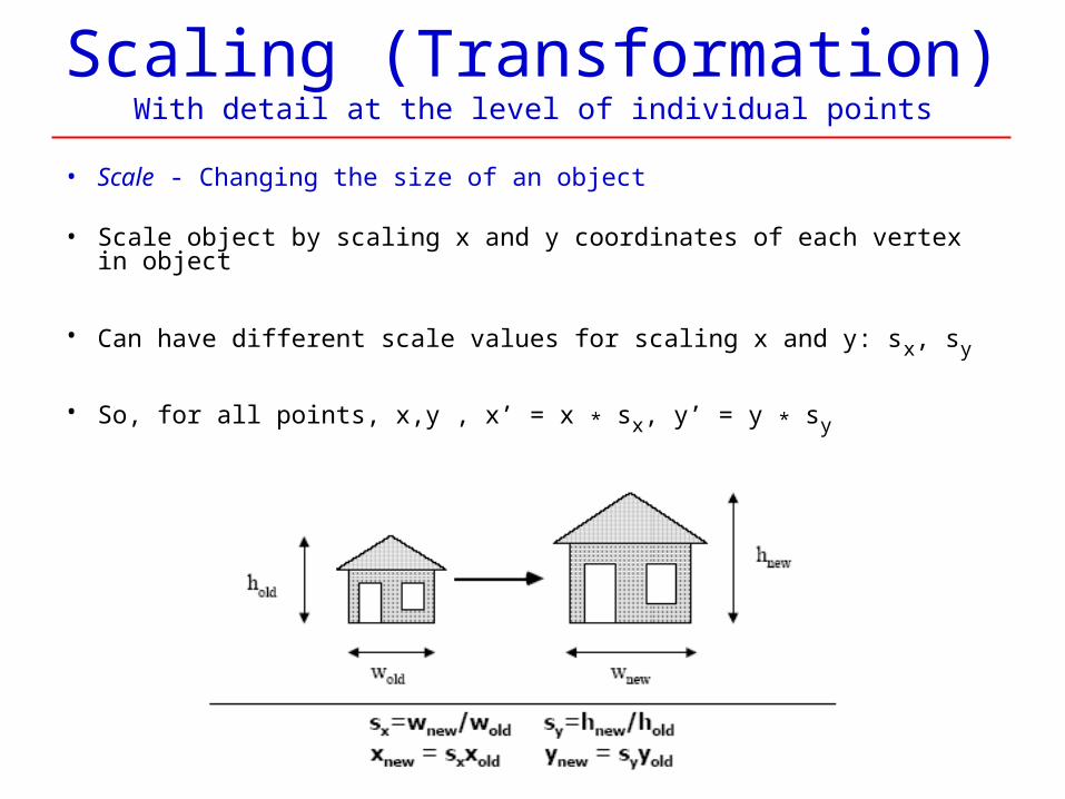
Scaling (Transformation)With detail at the level of individual points
• Scale - Changing the size of an object • Scale object by scaling x and y coordinates of each vertex in object
• Can have different scale values for scaling x and y: sx, sy
• So, for all points, x,y , x’ = x * sx, y’ = y * sy
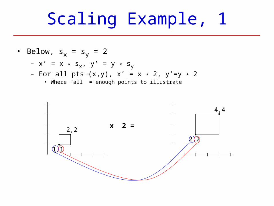
Scaling Example, 1
• Below, sx = sy = 2
– x’ = x * sx, y’ = y * sy
– For all pts (x,y), x’ = x * 2, y’=y * 2• Where “all” = enough points to illustrate
1,1
2,2
2,2
4,4
x 2 =
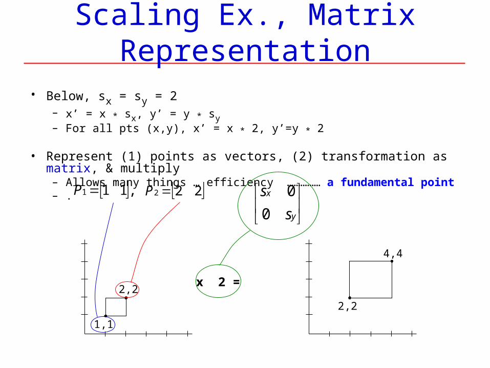
Scaling Ex., Matrix Representation
• Below, sx = sy = 2– x’ = x * sx, y’ = y * sy– For all pts (x,y), x’ = x * 2, y’=y * 2
• Represent (1) points as vectors, (2) transformation as matrix, & multiply– Allows many things … efficiency …………… a fundamental point– . 222 P
1,1
2,2
2,2
4,4
x 2 =
,111 P
y
x
s
s
0
0
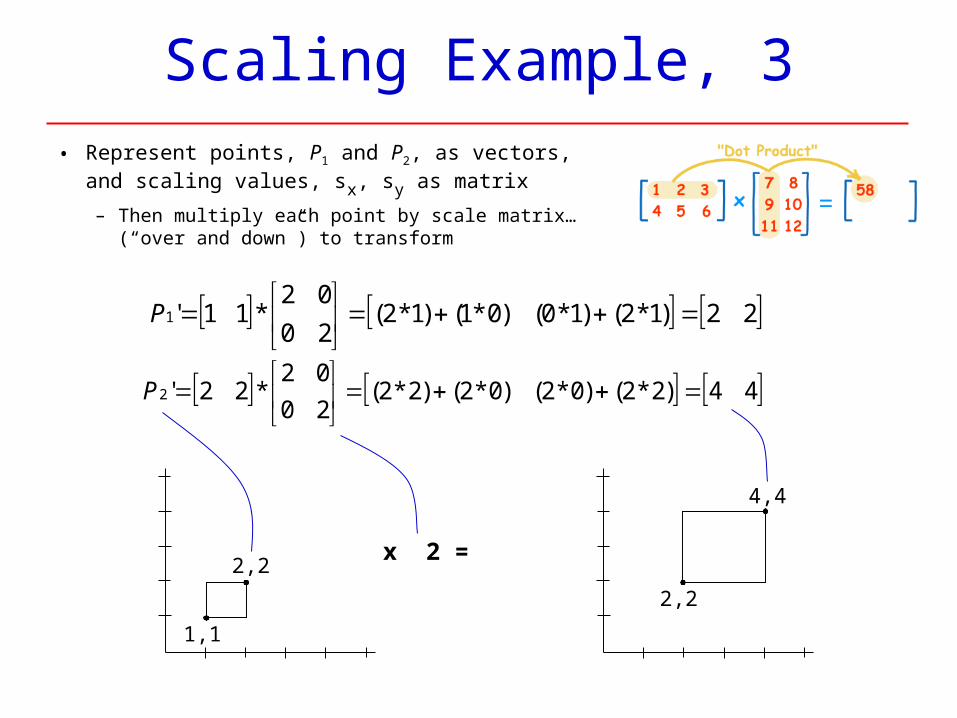
Scaling Example, 3
• Represent points, P1 and P2, as vectors, and scaling values, sx, sy as matrix
– Then multiply each point by scale matrix… (“over and down”) to transform
1,1
2,2
2,2
4,4
x 2 =
22)1*2()1*0()0*1()1*2(20
02*11'1
P
44)2*2()0*2()0*2()2*2(20
02*22'2
P
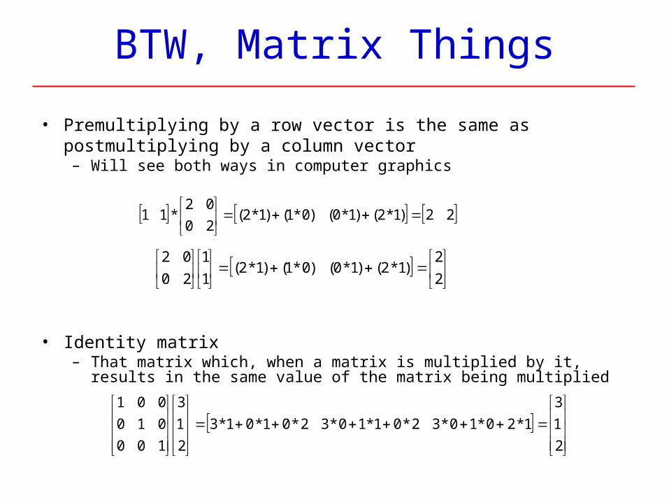
BTW, Matrix Things
• Premultiplying by a row vector is the same as postmultiplying by a column vector– Will see both ways in computer graphics
• Identity matrix– That matrix which, when a matrix is multiplied by it, results in the
same value of the matrix being multiplied
22)1*2()1*0()0*1()1*2(20
02*11
2
2)1*2()1*0()0*1()1*2(
1
1
20
02
2
1
3
1*20*10*32*01*10*32*01*01*3
2
1
3
100
010
001
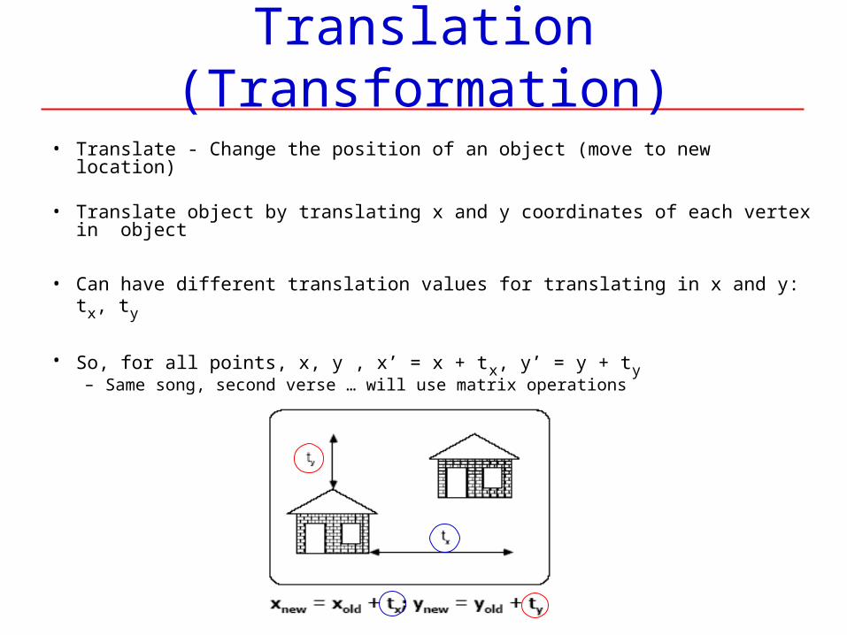
Translation (Transformation)
• Translate - Change the position of an object (move to new location) • Translate object by translating x and y coordinates of each vertex in
object
• Can have different translation values for translating in x and y: tx, ty
• So, for all points, x, y , x’ = x + tx, y’ = y + ty – Same song, second verse … will use matrix operations
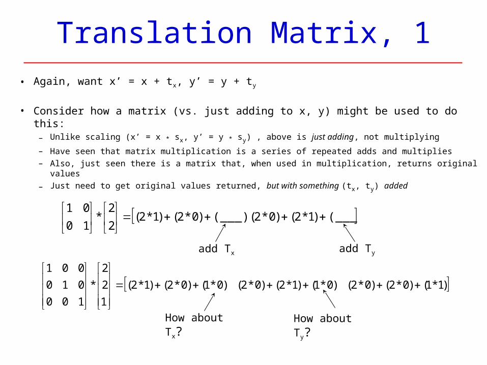
Translation Matrix, 1
• Again, want x’ = x + tx, y’ = y + ty
• Consider how a matrix (vs. just adding to x, y) might be used to do this:– Unlike scaling (x’ = x * sx, y’ = y * sy) , above is just adding, not multiplying
– Have seen that matrix multiplication is a series of repeated adds and multiplies– Also, just seen there is a matrix that, when used in multiplication, returns original values
– Just need to get original values returned, but with something (tx, ty) added
(___))1*2()0*2((___))0*2()1*2(2
2*
10
01
)1*1()0*2()0*2()0*1()1*2()0*2()0*1()0*2()1*2(
1
2
2
*
100
010
001
add Tx add Ty
How about Tx? How about Ty?
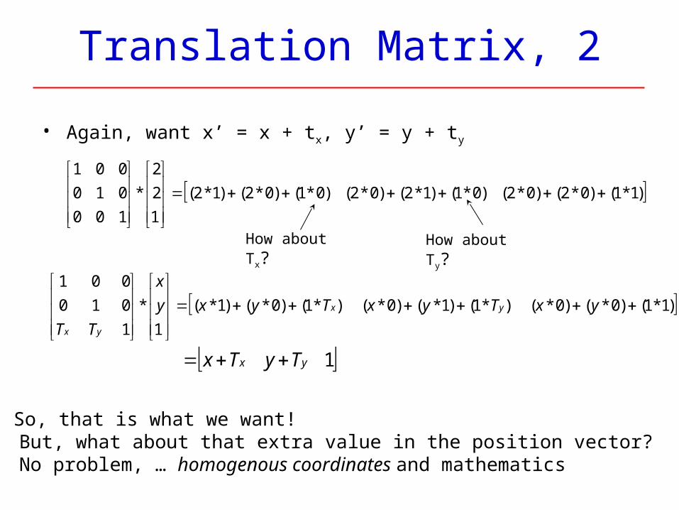
Translation Matrix, 2
• Again, want x’ = x + tx, y’ = y + ty
)1*1()0*2()0*2()0*1()1*2()0*2()0*1()0*2()1*2(
1
2
2
*
100
010
001
How about Tx? How about Ty?
)1*1()0*()0*()*1()1*()0*()*1()0*()1*(
1
*
1
010
001
yxTyxTyxy
x
TT
yx
yx
1yx TyTx
• So, that is what we want!• But, what about that extra value in the position vector?• No problem, … homogenous coordinates and mathematics
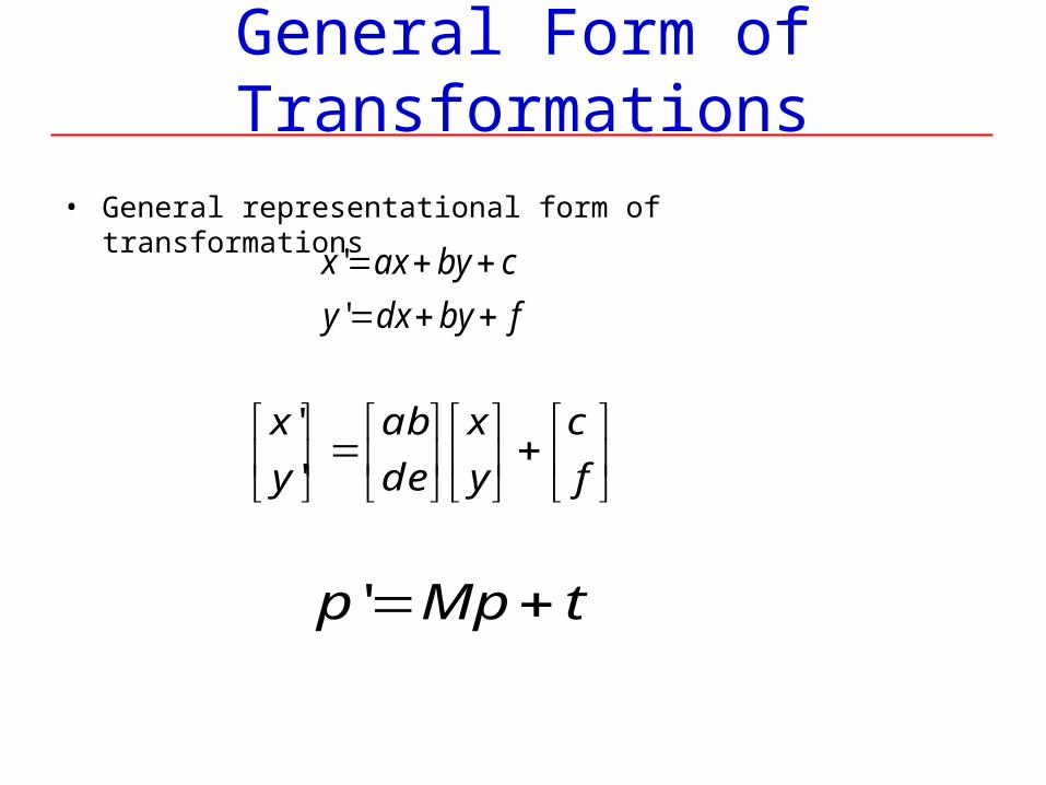
General Form of Transformations
• General representational form of transformations
fbydxy
cbyaxx
'
'
f
c
y
x
e
b
d
a
y
x
'
'
tMpp '
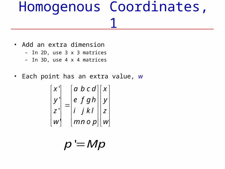
Homogenous Coordinates, 1
• Add an extra dimension– In 2D, use 3 x 3 matrices– In 3D, use 4 x 4 matrices
• Each point has an extra value, w
w
z
y
x
p
l
h
d
o
k
g
c
n
j
f
b
m
i
e
a
w
z
y
x
'
'
'
'
Mpp '
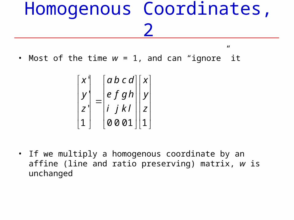
Homogenous Coordinates, 2
• Most of the time w = 1, and can “ignore” it
• If we multiply a homogenous coordinate by an affine (line and ratio preserving) matrix, w is unchanged
110001
'
'
'
z
y
x
l
h
d
k
g
c
j
f
b
i
e
a
z
y
x
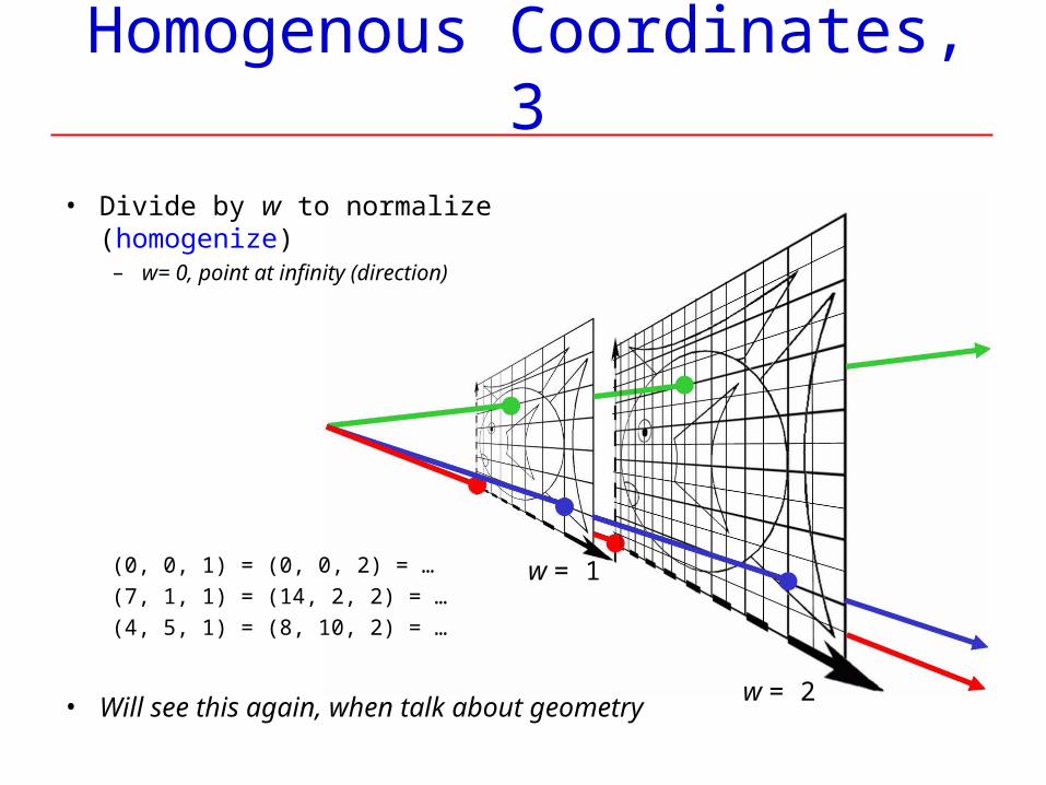
Homogenous Coordinates, 3
• Divide by w to normalize (homogenize)– w= 0, point at infinity (direction)
(0, 0, 1) = (0, 0, 2) = …
(7, 1, 1) = (14, 2, 2) = …
(4, 5, 1) = (8, 10, 2) = …
• Will see this again, when talk about geometry
w = 1
w = 2
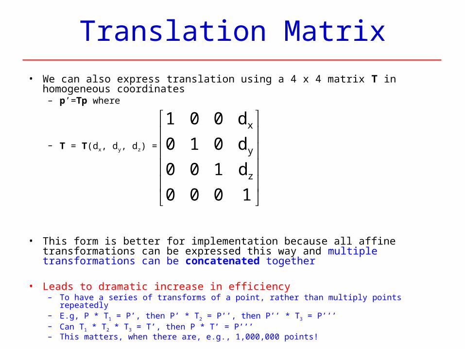
Translation Matrix
• We can also express translation using a 4 x 4 matrix T in homogeneous coordinates
– p’=Tp where
– T = T(dx, dy, dz) =
• This form is better for implementation because all affine transformations can be expressed this way and multiple transformations can be concatenated together
• Leads to dramatic increase in efficiency– To have a series of transforms of a point, rather than multiply points repeatedly– E.g, P * T1 = P’, then P’ * T2 = P’’, then P’’ * T3 = P’’’– Can T1 * T2 * T3 = T’, then P * T’ = P’’’ – This matters, when there are, e.g., 1,000,000 points!
1000
d100
d010
d001
z
y
x
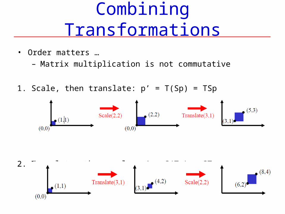
Combining Transformations
• Order matters …– Matrix multiplication is not commutative
1. Scale, then translate: p’ = T(Sp) = TSp
2. Translate, then scale: p’ = S(Tp) = STp
Order of Transformations
• Note that matrix on the right is the first applied
• Mathematically, the following are equivalent p’ = ABCp = A(B(Cp))
• Note - many references use column matrices to represent points. In terms of column matrices
p’T = pTCTBTAT
Affine TransformationsSome formality now
• Line preserving
• Characteristic of many physically important transformations– Rigid body transformations: rotation, translation– Scaling, shear
• Importance in graphics is that we need only transform endpoints of line segments and let implementation draw line segment between the transformed endpoints
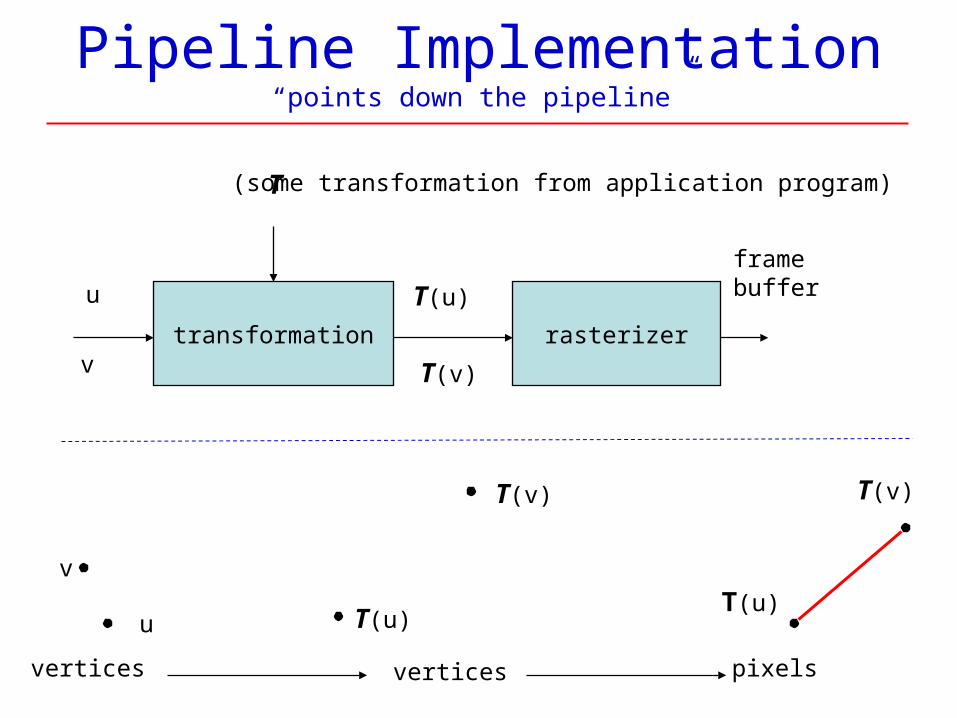
Pipeline Implementation“points down the pipeline”
transformation rasterizer
u
v
u
v
T
T(u)
T(v)
T(u)T(u)
T(v) T(v)
vertices vertices pixels
framebuffer
(some transformation from application program)
Notation (again)
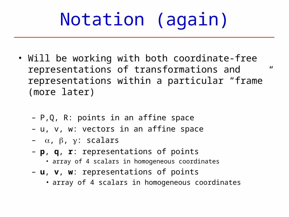
• Will be working with both coordinate-free representations of transformations and representations within a particular “frame” (more later)
– P,Q, R: points in an affine space– u, v, w: vectors in an affine space– , , : scalars– p, q, r: representations of points
• array of 4 scalars in homogeneous coordinates
– u, v, w: representations of points• array of 4 scalars in homogeneous coordinates
Translation
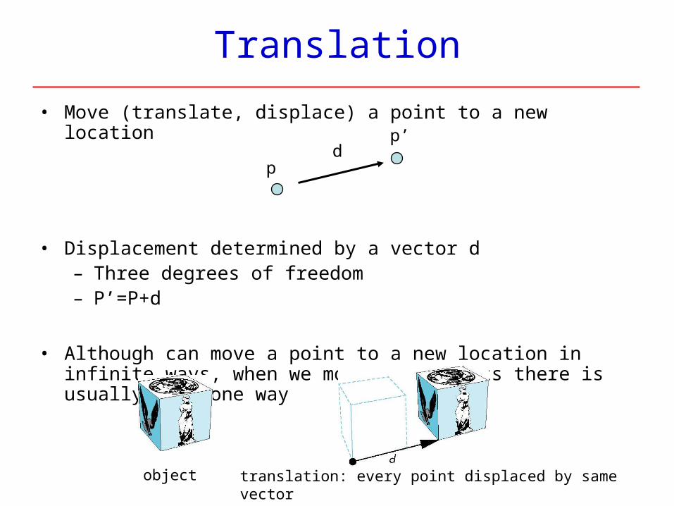
• Move (translate, displace) a point to a new location
• Displacement determined by a vector d– Three degrees of freedom– P’=P+d
• Although can move a point to a new location in infinite ways, when we move many points there is usually only one way
p
p’d
object translation: every point displaced by same vector
Rotation (2D) TransformationBriefly
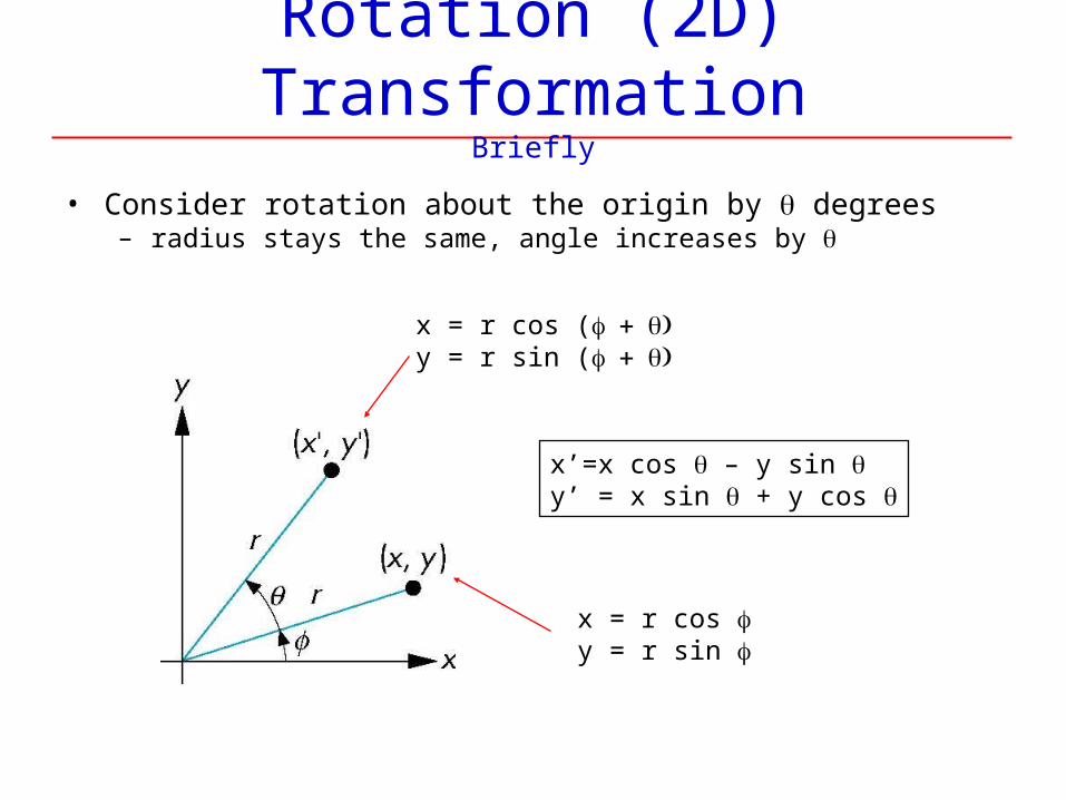
• Consider rotation about the origin by degrees– radius stays the same, angle increases by
x’=x cos – y sin y’ = x sin + y cos
x = r cos y = r sin
x = r cos (y = r sin (
Rotation about the z Axis3d homogenous coordinate representation
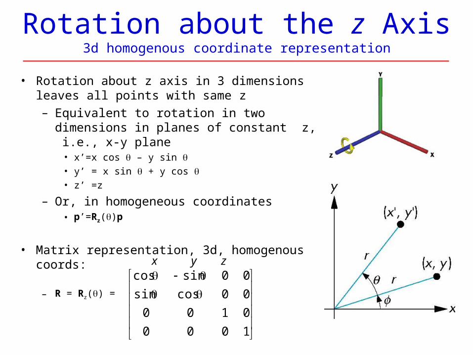
• Rotation about z axis in 3 dimensions leaves all points with same z– Equivalent to rotation in two dimensions in
planes of constant z, i.e., x-y plane• x’=x cos – y sin • y’ = x sin + y cos • z’ =z
– Or, in homogeneous coordinates• p’=Rz()p
• Matrix representation, 3d, homogenous coords:
– R = Rz() =
1000
0100
00 cossin
00sin cos x y z
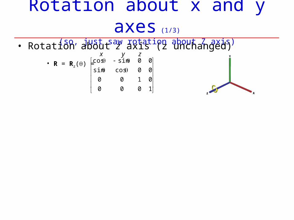
Rotation about x and y axes (1/3)
(so, just saw rotation about Z axis)
• Rotation about z axis (z unchanged)
• R = Rz() =
1000
0100
00 cossin
00sin cos x y z
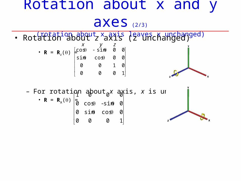
Rotation about x and y axes (2/3)
(rotation about x axis leaves x unchanged)
• Rotation about z axis (z unchanged)
• R = Rz() =
– For rotation about x axis, x is unchanged• R = Rx() =
1000
0 cos sin0
0 sin- cos0
0001
1000
0100
00 cossin
00sin cos x y z
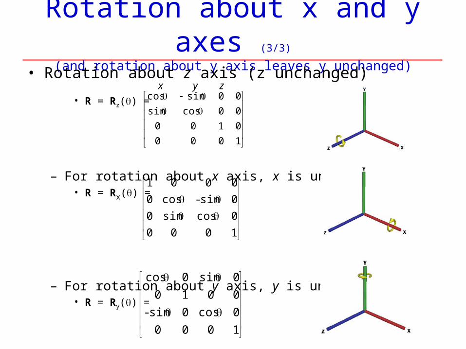
Rotation about x and y axes (3/3)
(and rotation about y axis leaves y unchanged)
• Rotation about z axis (z unchanged)
• R = Rz() =
– For rotation about x axis, x is unchanged• R = Rx() =
– For rotation about y axis, y is unchanged• R = Ry() =
1000
0 cos sin0
0 sin- cos0
0001
1000
0 cos0 sin-
0010
0 sin0 cos
1000
0100
00 cossin
00sin cos x y z
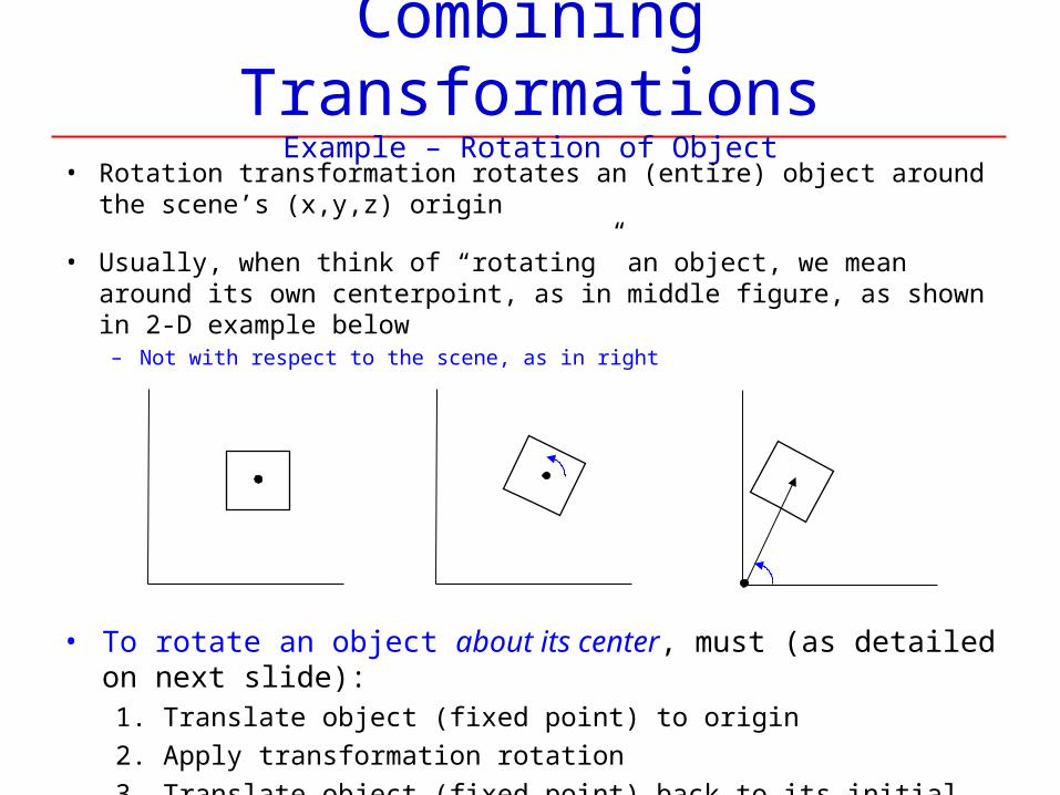
Combining TransformationsExample – Rotation of Object
• Rotation transformation rotates an (entire) object around the scene’s (x,y,z) origin
• Usually, when think of “rotating” an object, we mean around its own centerpoint, as in middle figure, as shown in 2-D example below
– Not with respect to the scene, as in right
• To rotate an object about its center, must (as detailed on next slide):1. Translate object (fixed point) to origin
2. Apply transformation rotation
3. Translate object (fixed point) back to its initial position
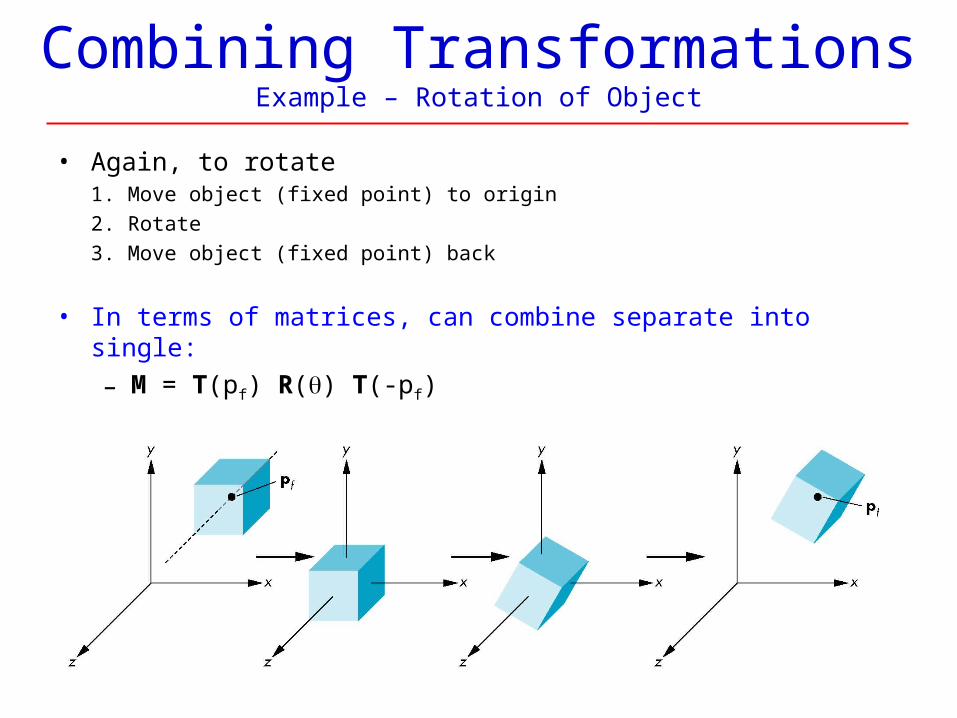
Combining TransformationsExample – Rotation of Object
• Again, to rotate1. Move object (fixed point) to origin
2. Rotate
3. Move object (fixed point) back
• In terms of matrices, can combine separate into single:
– M = T(pf) R() T(-pf)
OpenGL Example of using Transformation “Directly”
Maybe, or quickly, or “have a look at”, or later
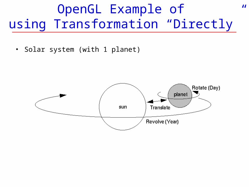
OpenGL Example of using Transformation “Directly”
• Solar system (with 1 planet)
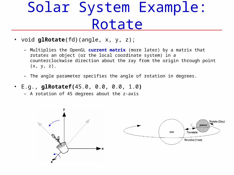
Solar System Example: Rotate
• void glRotate{fd}(angle, x, y, z);
– Multiplies the OpenGL current matrix (more later) by a matrix that rotates an object (or the local coordinate system) in a counterclockwise direction about the ray from the origin through point (x, y, z).
– The angle parameter specifies the angle of rotation in degrees.
• E.g., glRotatef(45.0, 0.0, 0.0, 1.0)– A rotation of 45 degrees about the z-axis
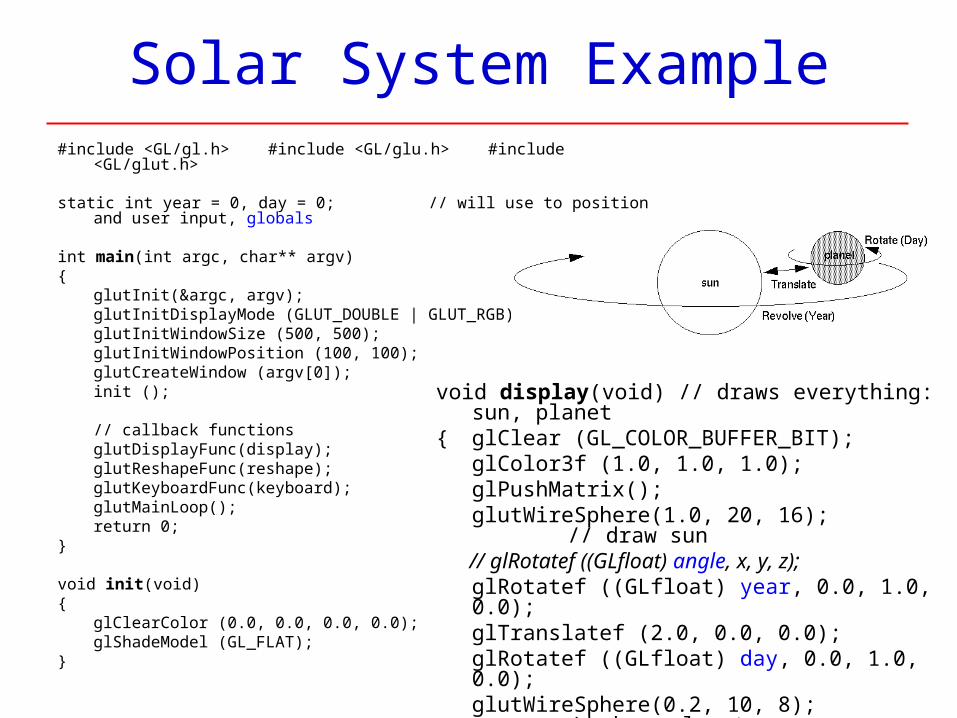
Solar System Example#include <GL/gl.h> #include <GL/glu.h> #include <GL/glut.h>
static int year = 0, day = 0; // will use to position and user input, globals
int main(int argc, char** argv){
glutInit(&argc, argv);glutInitDisplayMode (GLUT_DOUBLE | GLUT_RGB);glutInitWindowSize (500, 500);glutInitWindowPosition (100, 100); glutCreateWindow (argv[0]);init ();
// callback functionsglutDisplayFunc(display);glutReshapeFunc(reshape); glutKeyboardFunc(keyboard); glutMainLoop(); return 0;
}
void init(void){
glClearColor (0.0, 0.0, 0.0, 0.0); glShadeModel (GL_FLAT);
}
void display(void) // draws everything: sun, planet{ glClear (GL_COLOR_BUFFER_BIT);
glColor3f (1.0, 1.0, 1.0); glPushMatrix();glutWireSphere(1.0, 20, 16); // draw sun
// glRotatef ((GLfloat) angle, x, y, z); glRotatef ((GLfloat) year, 0.0, 1.0, 0.0); glTranslatef (2.0, 0.0, 0.0);glRotatef ((GLfloat) day, 0.0, 1.0, 0.0);glutWireSphere(0.2, 10, 8); // draw planetglutSwapBuffers();
}
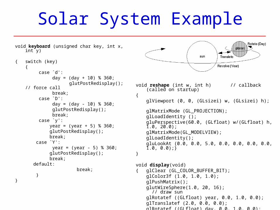
Solar System Examplevoid keyboard (unsigned char key, int x, int y)
{ switch (key) { case `d': day = (day + 10) % 360;
glutPostRedisplay(); // force call break; case `D': day = (day - 10) % 360; glutPostRedisplay(); break; case `y': year = (year + 5) % 360; glutPostRedisplay(); break; case `Y': year = (year - 5) % 360; glutPostRedisplay(); break; default:
break; }
}
void reshape (int w, int h) // callback (called on startup){
glViewport (0, 0, (GLsizei) w, (GLsizei) h); glMatrixMode (GL_PROJECTION); glLoadIdentity ();gluPerspective(60.0, (GLfloat) w/(GLfloat) h, 1.0, 20.0);glMatrixMode(GL_MODELVIEW);glLoadIdentity();gluLookAt (0.0, 0.0, 5.0, 0.0, 0.0, 0.0, 0.0, 1.0, 0.0);}
}
void display(void){ glClear (GL_COLOR_BUFFER_BIT);
glColor3f (1.0, 1.0, 1.0); glPushMatrix();glutWireSphere(1.0, 20, 16); // draw sun glRotatef ((GLfloat) year, 0.0, 1.0, 0.0); glTranslatef (2.0, 0.0, 0.0);glRotatef ((GLfloat) day, 0.0, 1.0, 0.0);glutWireSphere(0.2, 10, 8); // draw smaller planetglutSwapBuffers();
}
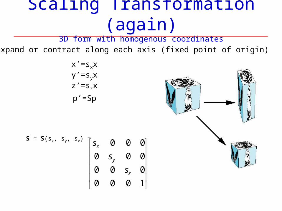
Scaling Transformation (again)3D form with homogenous coordinates
1000
000
000
000
z
y
x
s
s
sS = S(sx, sy, sz) =
x’=sxxy’=syxz’=szx
p’=Sp
• Expand or contract along each axis (fixed point of origin)
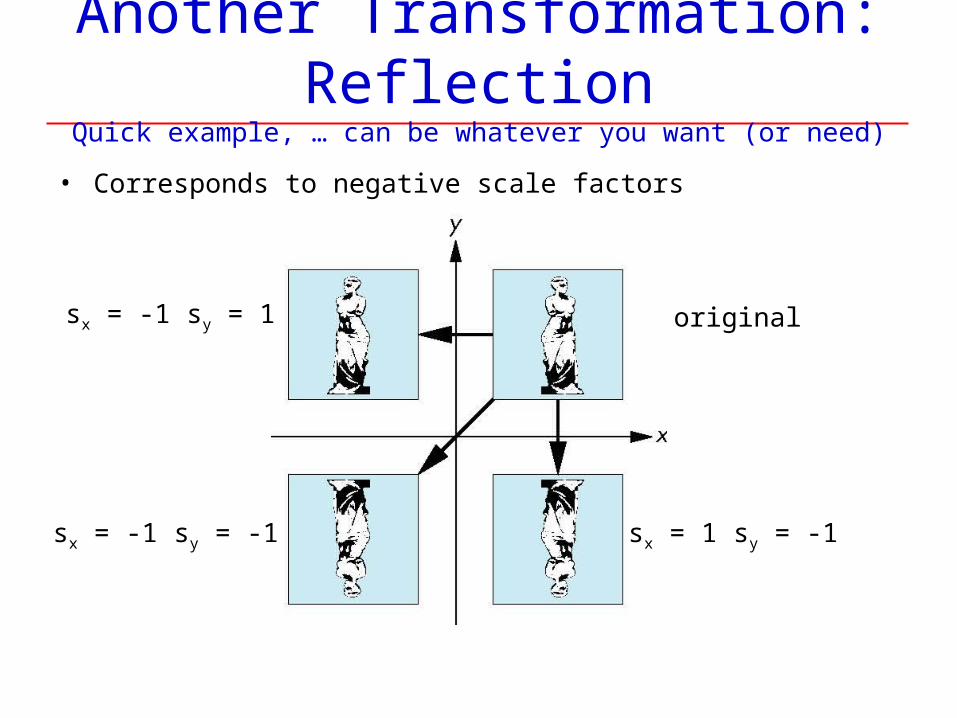
Another Transformation: ReflectionQuick example, … can be whatever you want (or need)
• Corresponds to negative scale factors
originalsx = -1 sy = 1
sx = -1 sy = -1 sx = 1 sy = -1
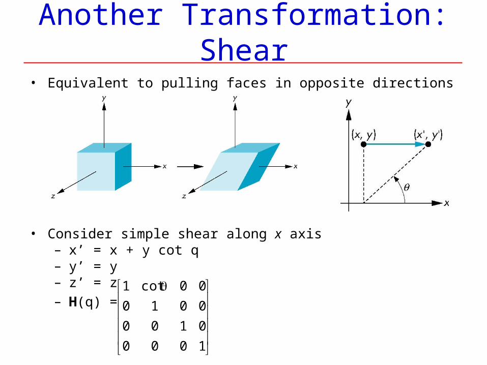
Another Transformation: Shear
• Equivalent to pulling faces in opposite directions
• Consider simple shear along x axis– x’ = x + y cot q– y’ = y– z’ = z– H(q) =
1000
0100
0010
00cot 1
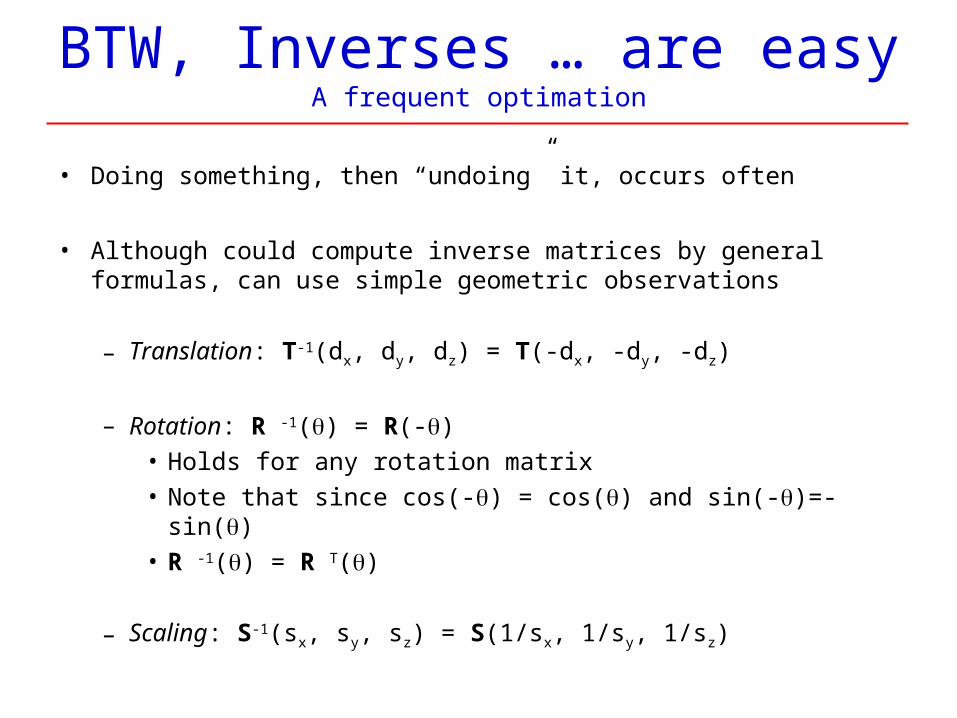
BTW, Inverses … are easyA frequent optimation
• Doing something, then “undoing” it, occurs often
• Although could compute inverse matrices by general formulas, can use simple geometric observations
– Translation: T-1(dx, dy, dz) = T(-dx, -dy, -dz)
– Rotation: R -1() = R(-)• Holds for any rotation matrix• Note that since cos(-) = cos() and sin(-)=-sin()• R -1() = R T()
– Scaling: S-1(sx, sy, sz) = S(1/sx, 1/sy, 1/sz)
Concatenation and Efficiency
• This is a big idea! …
Concatenation and Efficiency
• This is a big idea! …
• Recall, example of rotation of an object
• We can form arbitrary affine transformation matrices by multiplying together rotation, translation, and scaling matrices
• Because the same transformation is applied to many vertices, – cost of forming a matrix M=ABCD is not significant compared to
the cost of computing Mp for many vertices p• Computing comparative costs is frequent text exercise
• The difficult part is how to form a desired transformation from the specifications in the application
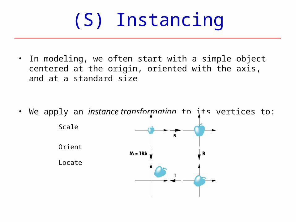
(S) Instancing
• In modeling, we often start with a simple object centered at the origin, oriented with the axis, and at a standard size
• We apply an instance transformation to its vertices to:
Scale
Orient
Locate
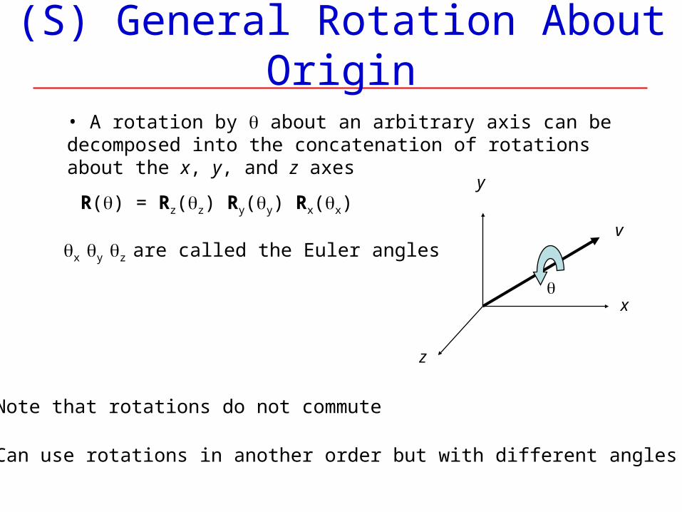
(S) General Rotation About Origin
x
z
y
v
• A rotation by about an arbitrary axis can be decomposed into the concatenation of rotations about the x, y, and z axes
R() = Rz(z) Ry(y) Rx(x)
x y z are called the Euler angles
• Note that rotations do not commute
• Can use rotations in another order but with different angles
OpenGL Geometry Transformation
• Finally, … we have the details of the several transformations in OpenGL viewing
• To summarize … (and introduce one more analogy …)
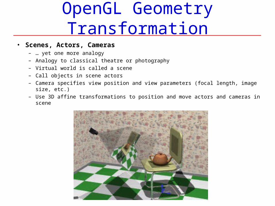
OpenGL Geometry Transformation
• Scenes, Actors, Cameras– … yet one more analogy – Analogy to classical theatre or photography– Virtual world is called a scene– Call objects in scene actors– Camera specifies view position and view parameters (focal length, image size, etc.)– Use 3D affine transformations to position and move actors and cameras in scene
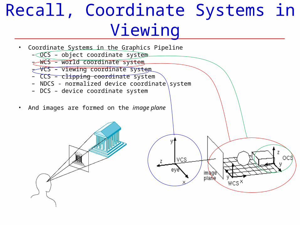
Recall, Coordinate Systems in Viewing
• Coordinate Systems in the Graphics Pipeline – OCS – object coordinate system – WCS – world coordinate system – VCS – viewing coordinate system – CCS – clipping coordinate system – NDCS - normalized device coordinate system – DCS – device coordinate system
• And images are formed on the image plane
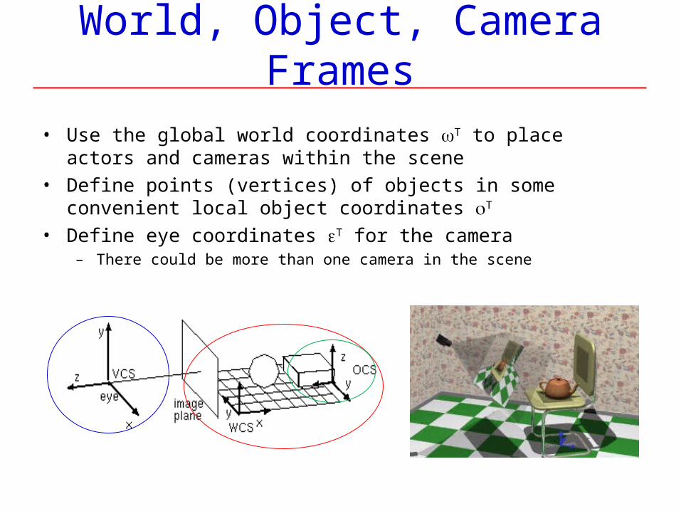
World, Object, Camera Frames
• Use the global world coordinates T to place actors and cameras within the scene
• Define points (vertices) of objects in some convenient local object coordinates T
• Define eye coordinates T for the camera– There could be more than one camera in the scene
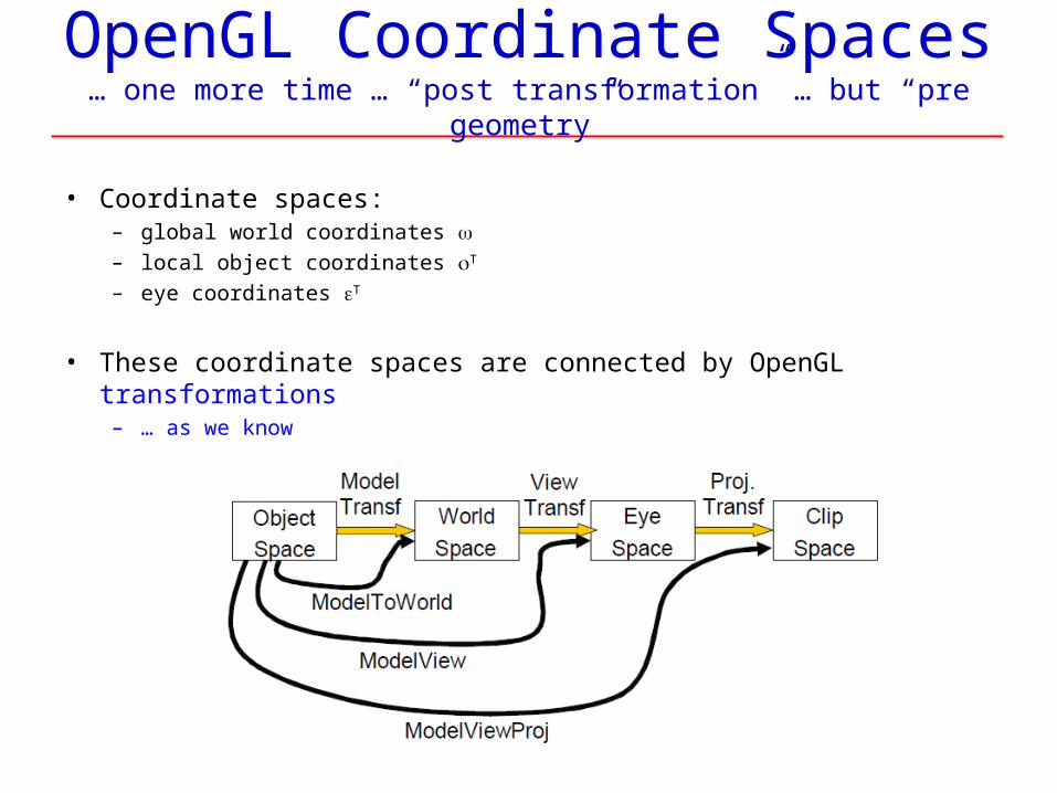
OpenGL Coordinate Spaces… one more time … “post transformation” … but “pre geometry”
• Coordinate spaces:– global world coordinates – local object coordinates T
– eye coordinates T
• These coordinate spaces are connected by OpenGL transformations– … as we know
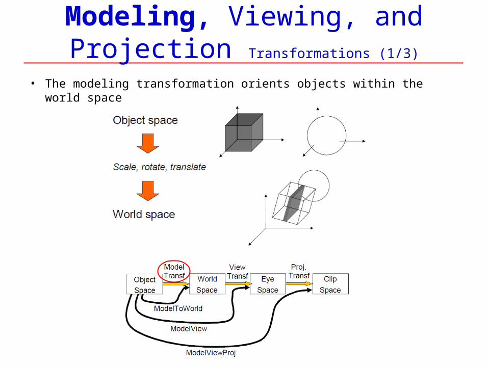
Modeling, Viewing, and Projection Transformations (1/3)
• The modeling transformation orients objects within the world space
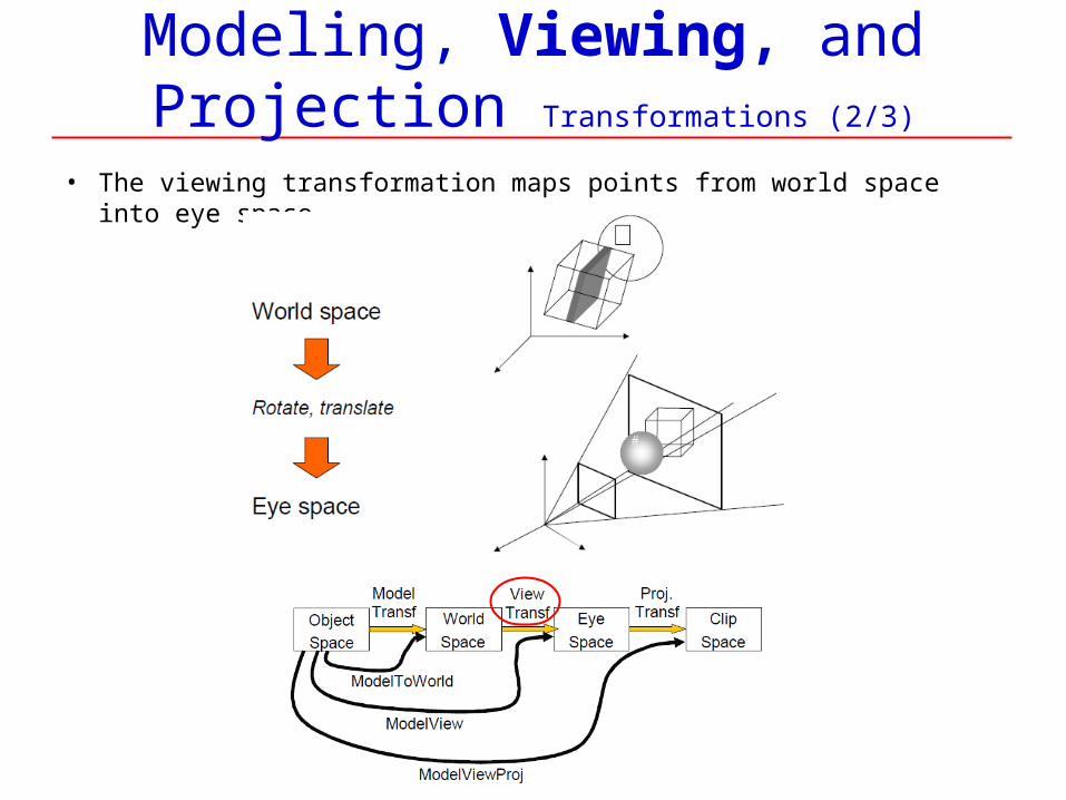
Modeling, Viewing, and Projection Transformations (2/3)
• The viewing transformation maps points from world space into eye space
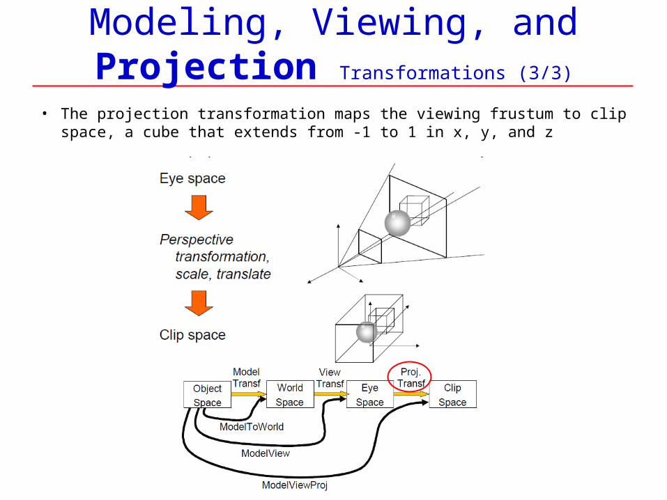
Modeling, Viewing, and Projection Transformations (3/3)
• The projection transformation maps the viewing frustum to clip space, a cube that extends from -1 to 1 in x, y, and z
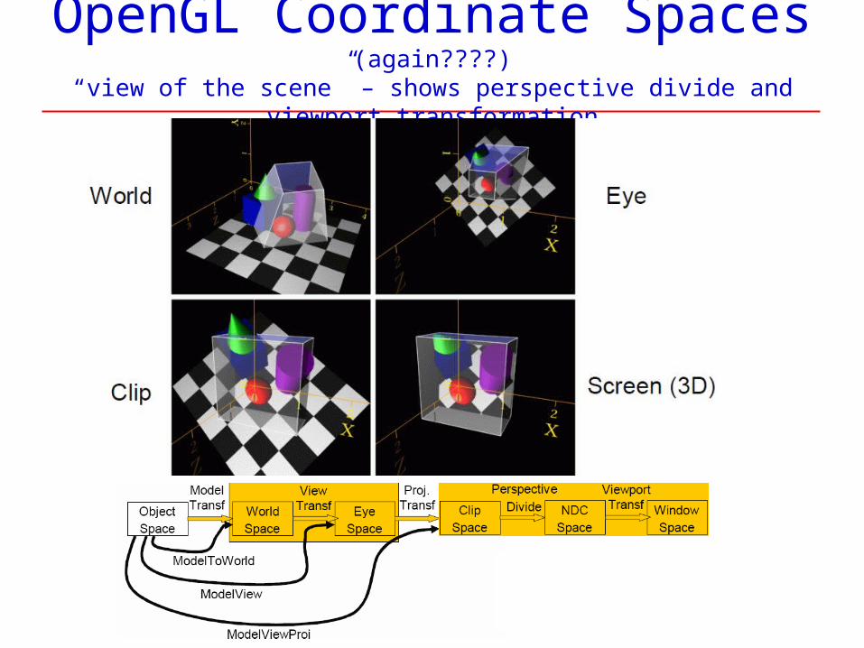
OpenGL Coordinate Spaces (again????)
“view of the scene” – shows perspective divide and viewport transformation
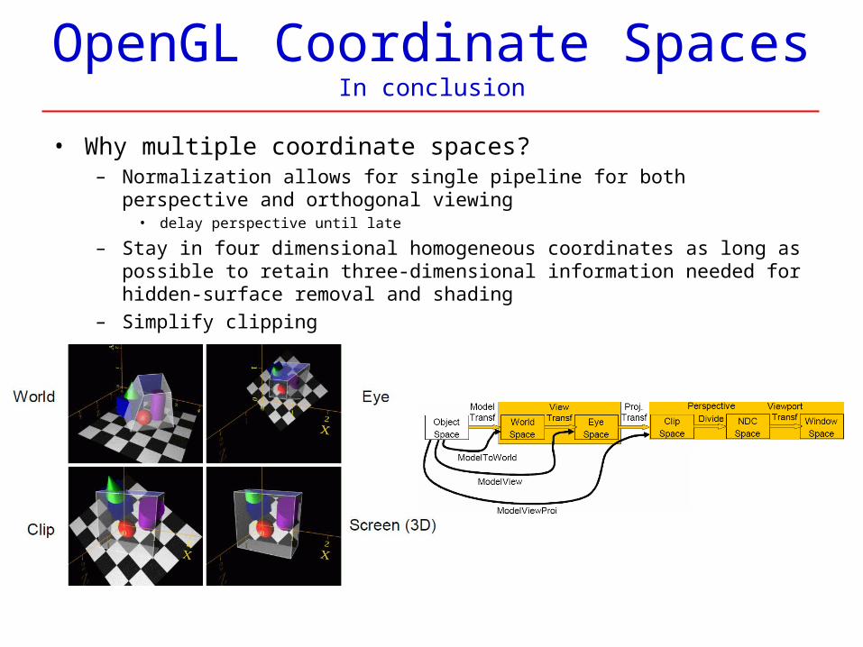
OpenGL Coordinate SpacesIn conclusion
• Why multiple coordinate spaces?– Normalization allows for single pipeline for both perspective and orthogonal
viewing • delay perspective until late
– Stay in four dimensional homogeneous coordinates as long as possible to retain three-dimensional information needed for hidden-surface removal and shading
– Simplify clipping

Geometry
Geometry: Basic ElementsWe’ll “just do it”
• Geometry is the study of relationships among objects in an n-dimensional space
– In cg, interested in objects that exist in three dimensions
• Want minimum set of primitives from which can build more sophisticated objects
• Will need three basic elements:– Scalars, Vectors, Points
• Coordinate-Free Geometry – important for cg
– “Simple geometry” - Cartesian approach• Points were at locations in space p=(x,y,z)• Derived results by algebraic manipulations involving these coordinates
– This approach was nonphysical• Physically, points exist regardless of location of an arbitrary coordinate system• Most geometric results are independent of the coordinate system• Example from Euclidean geometry: two triangles are identical if two
corresponding sides and the angle between them are identical
Vector, Affine, and Euclidean Spaces
• Different “spaces”
• Vector space– Contains 2 distinct entities: vectors and scalars– Supports 2 operations: addition and multiplication– Scalar-vector multiplication and vector-vector addition
• Affine space– Extension of vector space– Supports
• Vector-point addition that produces a new point• Point-point subtraction that produces a vector
• Euclidean space– Extension of vector space that adds a measure of size or distance
(Review)Geometry 1: Basic Geometric Elements
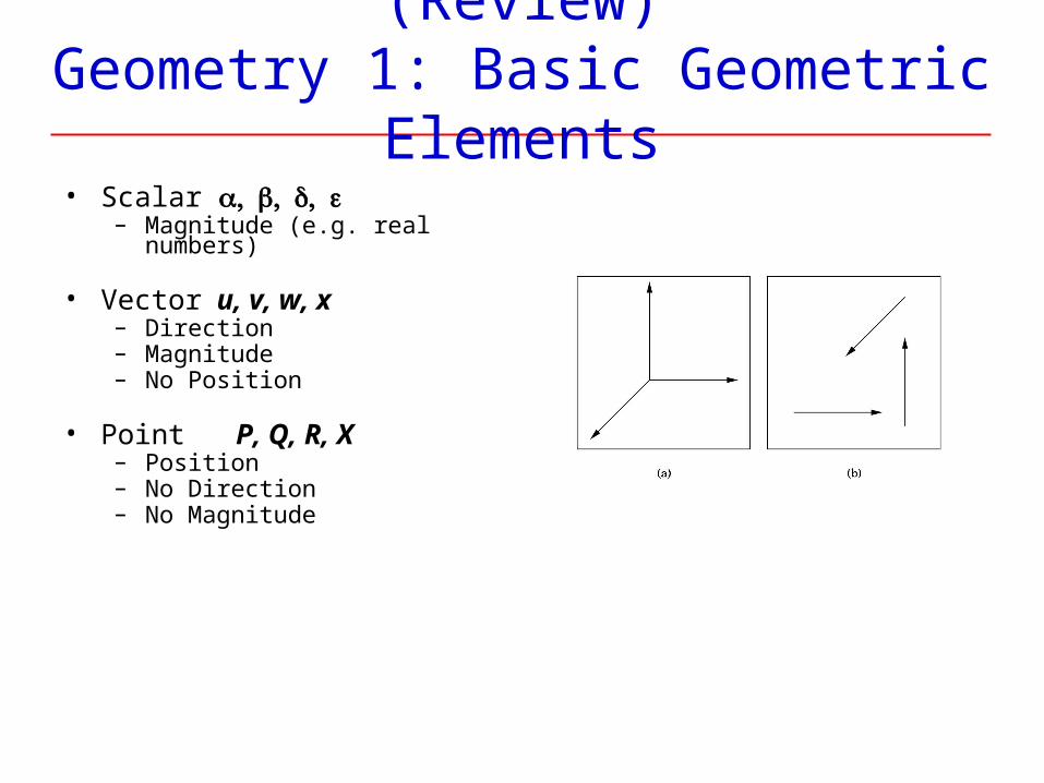
• Scalar – Magnitude (e.g. real numbers)
• Vector u, v, w, x– Direction– Magnitude– No Position
• Point P, Q, R, X– Position– No Direction– No Magnitude
(Review)Geometry 1: Scalars
• Scalars can be defined as members of sets which can be combined by two operations (addition and multiplication) obeying some fundamental axioms (associativity, commutivity, inverses)
• Examples include the real and complex number systems under the ordinary rules with which we are familiar
• Scalars alone have no geometric properties
• Operations (what you’d expect):– Addition:
• Additive identity: zero• Additive inverse: - • Subtraction defined in terms of additive inverse
– Multiplication: • Multiplicative identity: 1• Multiplicative inverse: 1/ • Division defined in terms of multiplicative inverse
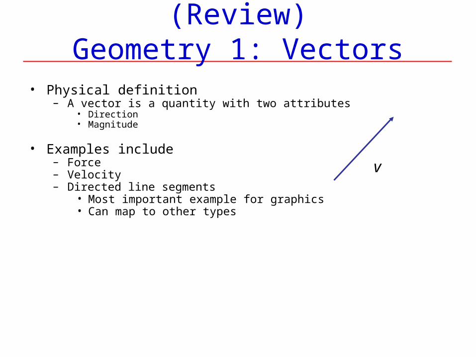
(Review)Geometry 1: Vectors
• Physical definition– A vector is a quantity with two attributes
• Direction• Magnitude
• Examples include– Force– Velocity– Directed line segments
• Most important example for graphics• Can map to other types
v
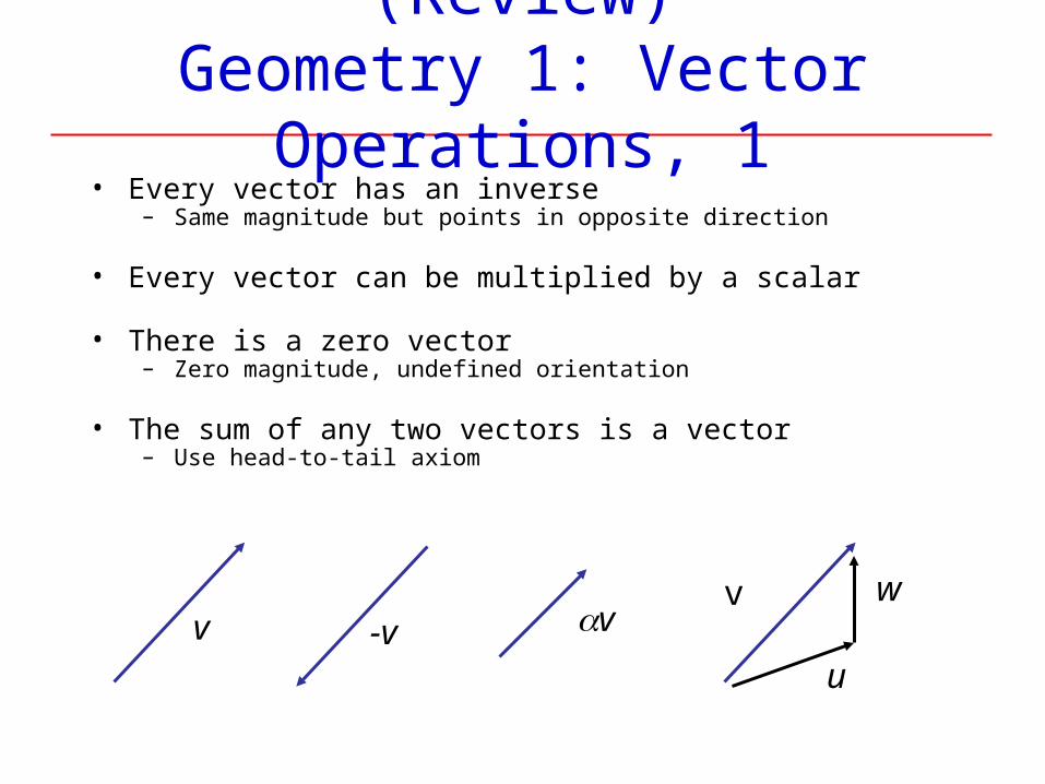
(Review)Geometry 1: Vector Operations, 1
• Every vector has an inverse– Same magnitude but points in opposite direction
• Every vector can be multiplied by a scalar
• There is a zero vector– Zero magnitude, undefined orientation
• The sum of any two vectors is a vector– Use head-to-tail axiom
v -v vv
u
w
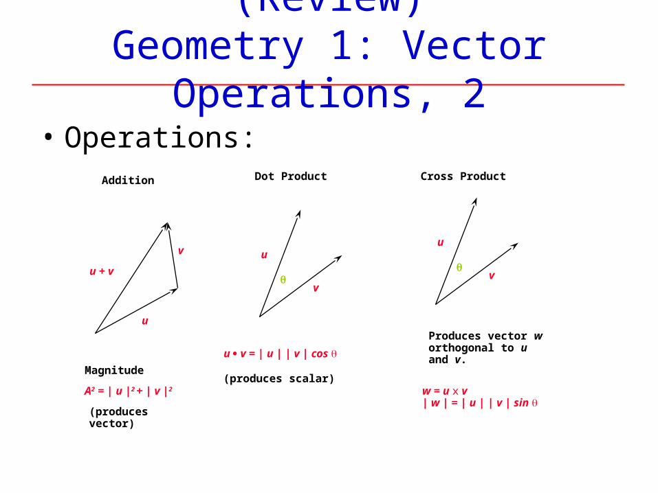
(Review)Geometry 1: Vector Operations, 2
• Operations:Addition
u
v
u + v
A2 = | u |2 + | v |2
Magnitude
(producesvector)
Dot Product
u
v
u v = | u | | v | cos
(produces scalar)
Cross Product
u
v
w = u x v| w | = | u | | v | sin
Produces vector worthogonal to u and v.
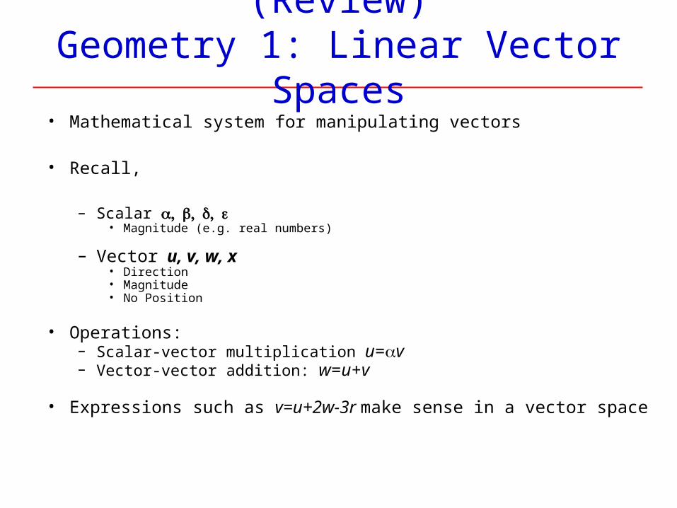
(Review)Geometry 1: Linear Vector Spaces• Mathematical system for manipulating vectors
• Recall,
– Scalar • Magnitude (e.g. real numbers)
– Vector u, v, w, x• Direction• Magnitude• No Position
• Operations:– Scalar-vector multiplication u=v– Vector-vector addition: w=u+v
• Expressions such as v=u+2w-3r make sense in a vector space
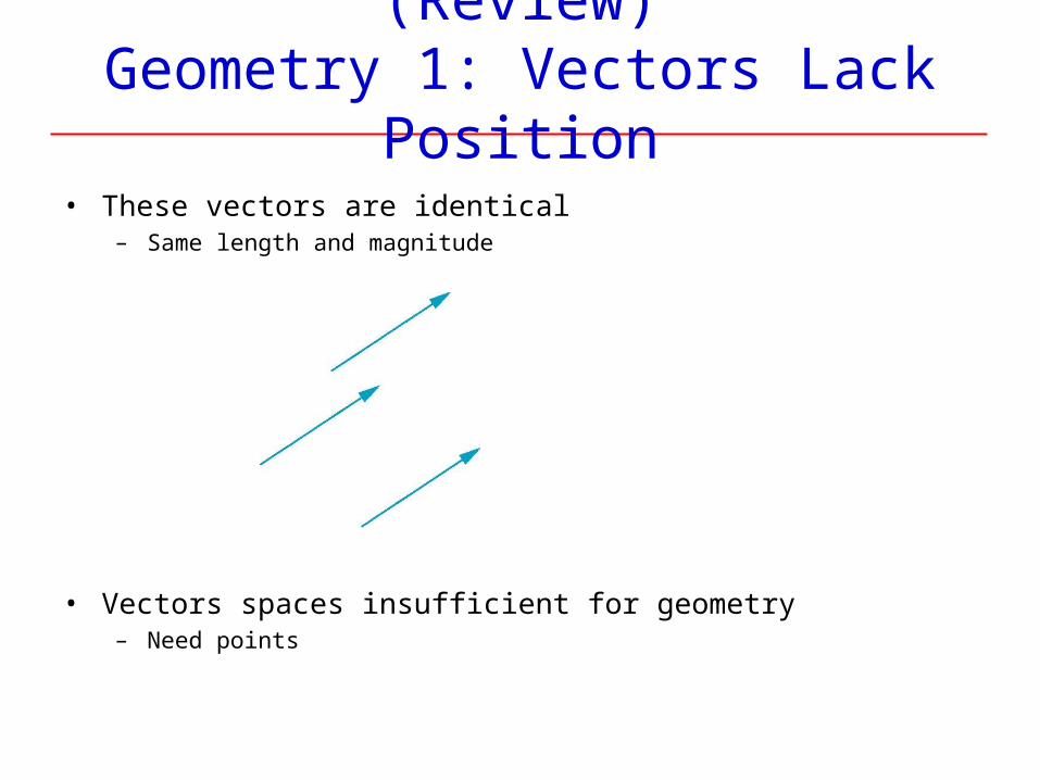
(Review)Geometry 1: Vectors Lack Position
• These vectors are identical– Same length and magnitude
• Vectors spaces insufficient for geometry– Need points
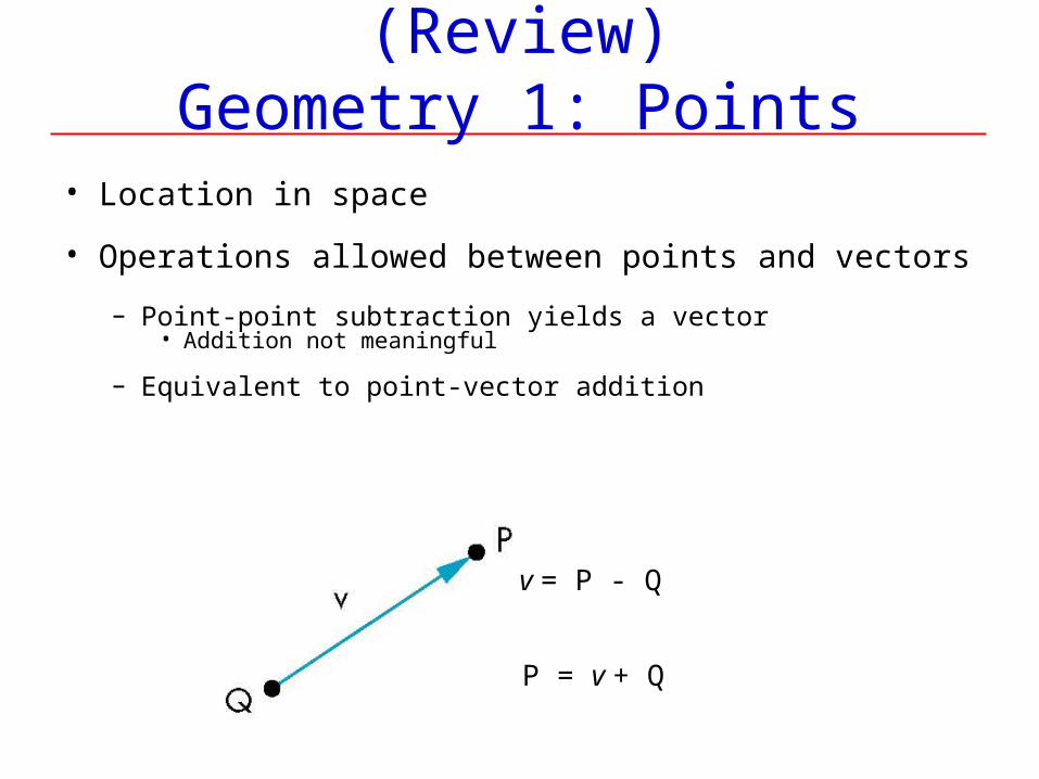
(Review)Geometry 1: Points
• Location in space
• Operations allowed between points and vectors
– Point-point subtraction yields a vector• Addition not meaningful
– Equivalent to point-vector addition
P = v + Q
v = P - Q
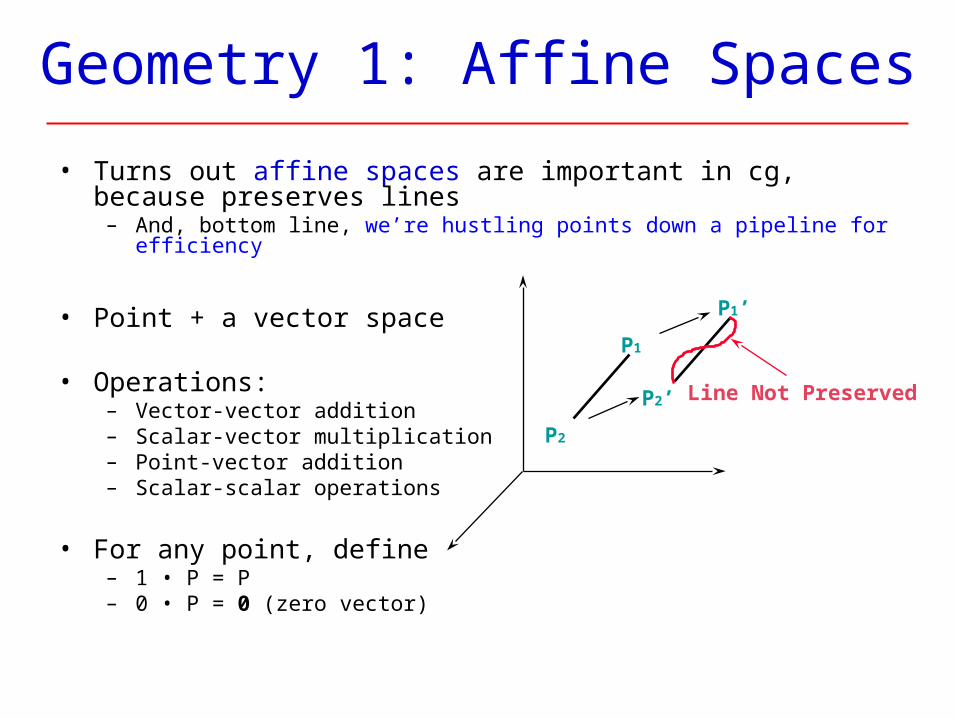
Geometry 1: Affine Spaces
• Turns out affine spaces are important in cg, because preserves lines
– And, bottom line, we’re hustling points down a pipeline for efficiency
• Point + a vector space
• Operations:– Vector-vector addition– Scalar-vector multiplication– Point-vector addition– Scalar-scalar operations
• For any point, define– 1 • P = P– 0 • P = 0 (zero vector)
P1’
P2’
P1
P2
Line Not Preserved
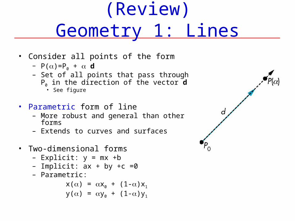
(Review)Geometry 1: Lines
• Consider all points of the form– P()=P0 + d– Set of all points that pass through P0 in the
direction of the vector d • See figure
• Parametric form of line– More robust and general than other forms– Extends to curves and surfaces
• Two-dimensional forms– Explicit: y = mx +b– Implicit: ax + by +c =0– Parametric: x() = x0 + (1-)x1
y() = y0 + (1-)y1
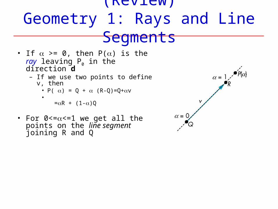
(Review)Geometry 1: Rays and Line Segments
• If >= 0, then P() is the ray leaving P0 in the direction d– If we use two points to define v,
then• P( ) = Q + (R-Q)=Q+v• =R + (1-)Q
• For 0<=<=1 we get all the points on the line segment joining R and Q
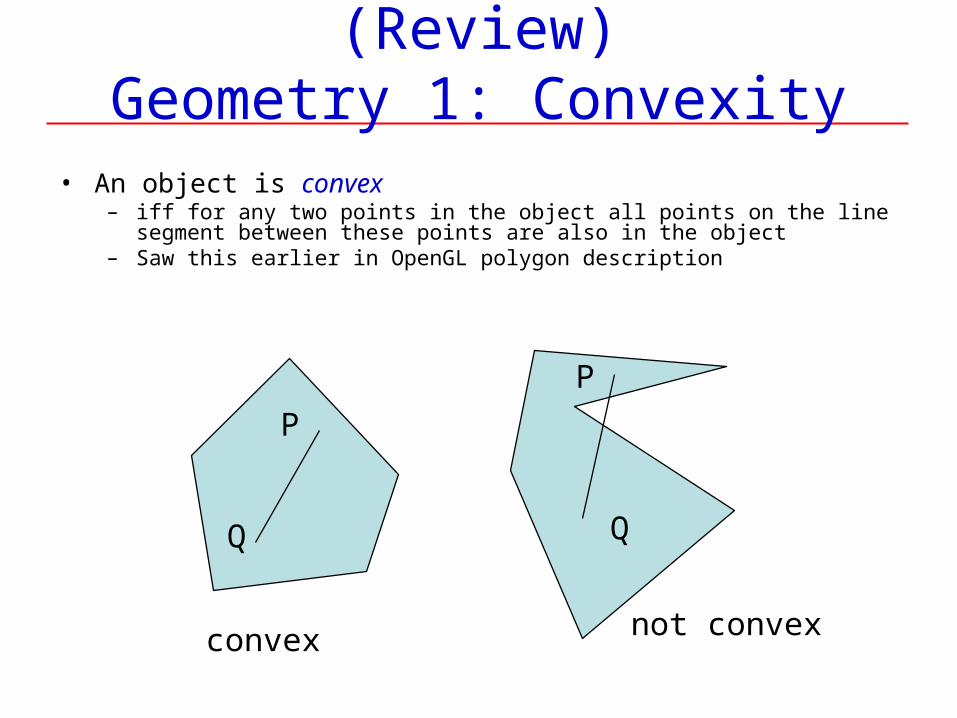
(Review)Geometry 1: Convexity
• An object is convex – iff for any two points in the object all points on the line segment between these
points are also in the object– Saw this earlier in OpenGL polygon description
P
Q Q
P
convex not convex
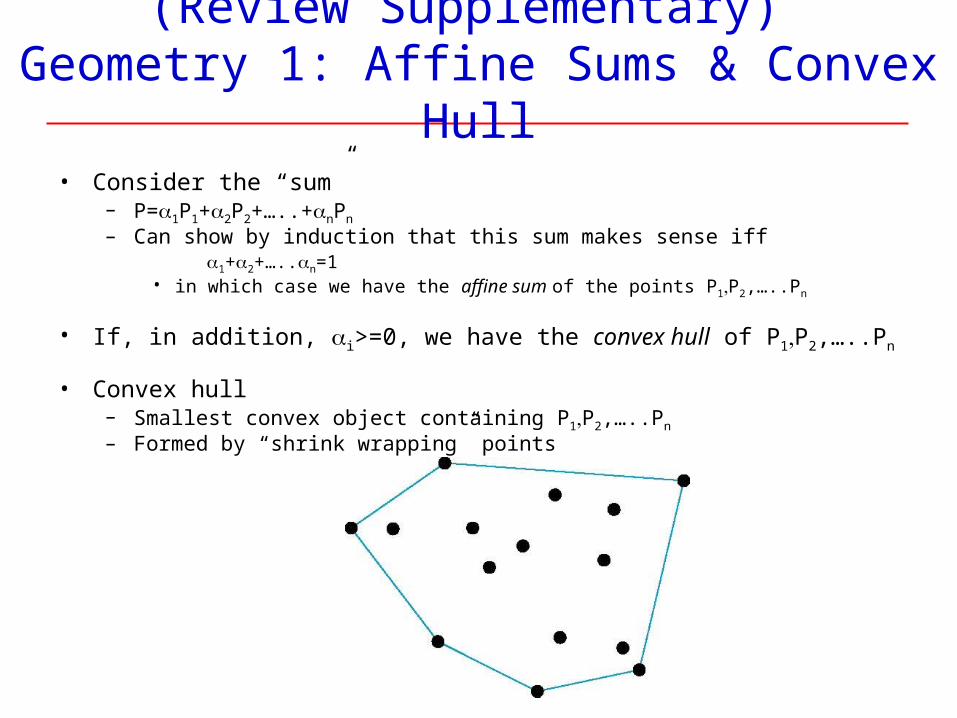
(Review Supplementary) Geometry 1: Affine Sums & Convex Hull
• Consider the “sum”– P=1P1+2P2+…..+nPn
– Can show by induction that this sum makes sense iff1+2+…..n=1• in which case we have the affine sum of the points P1P2,…..Pn
• If, in addition, i>=0, we have the convex hull of P1P2,…..Pn
• Convex hull– Smallest convex object containing P1P2,…..Pn
– Formed by “shrink wrapping” points
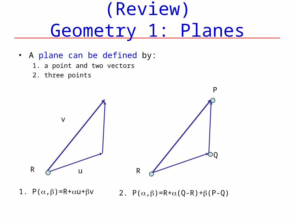
(Review)Geometry 1: Planes
• A plane can be defined by: 1. a point and two vectors
2. three points
1. P(,)=R+u+v 2. P(,)=R+(Q-R)+(P-Q)
u
v
R
P
R
Q
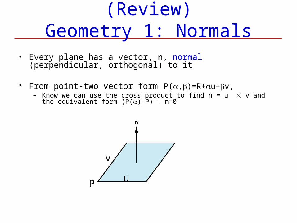
(Review)Geometry 1: Normals
• Every plane has a vector, n, normal (perpendicular, orthogonal) to it
• From point-two vector form P(,)=R+u+v, – Know we can use the cross product to find n = u v and the equivalent form
(P()-P) n=0
u
v
P
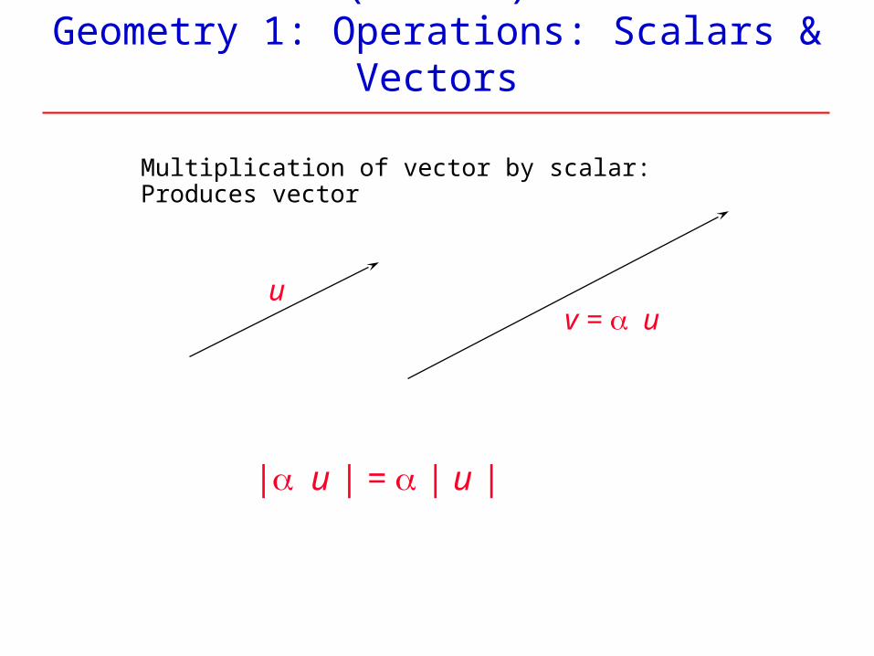
(Review)Geometry 1: Operations: Scalars & Vectors
Multiplication of vector by scalar:Produces vector
uv = u
|u | = | u |
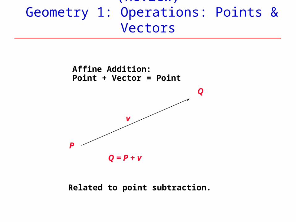
(Review) Geometry 1: Operations: Points & Vectors
Affine Addition:Point + Vector = Point
P
Q
v
Q = P + v
Related to point subtraction.
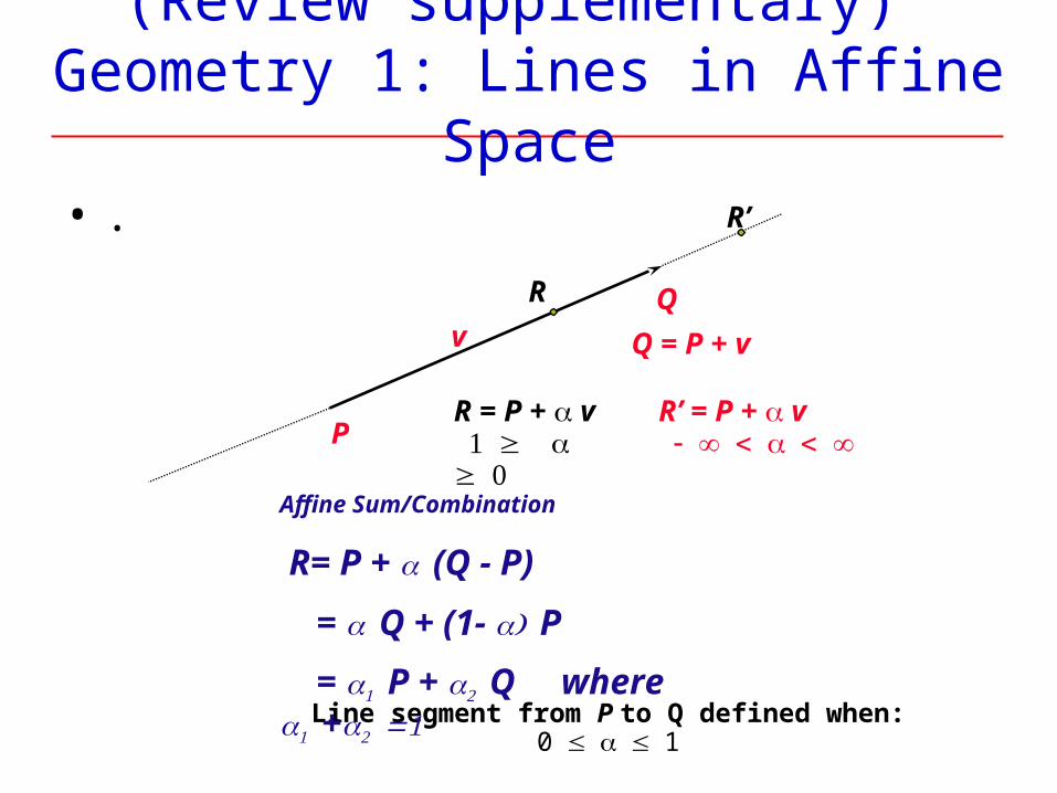
(Review supplementary) Geometry 1: Lines in Affine Space
• .
P
Qv Q = P + v
R
R = P + v
R’
Line segment from P to Q defined when: 01
R’ = P + v
Affine Sum/Combination
R= P + (Q - P)
= Q + (1- P
= P + Q where +
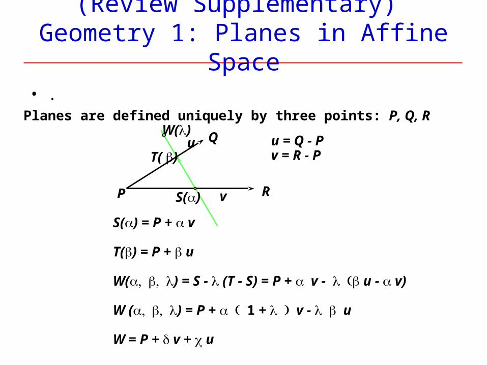
(Review Supplementary) Geometry 1: Planes in Affine Space
• .Planes are defined uniquely by three points: P, Q, R
P
Q
R
u
v
T( )
S()
S() = P + v
T() = P + u
W() = S - (T - S) = P + v - u - v)
W () = P + 1 + v - u
W = P + v + u
W()u = Q - Pv = R - P
Geometry 2: Basis, Coordinate Systems
Geometry 2: Basis, Coordinate Systems
• Will look at things such as dimension and basis– Concepts familiar, mathematic treatment
• Also, – coordinate systems for representing vectors spaces and – frames for representing affine spaces
• Discuss change of frames and bases– Mathematical elements of “transformations” we just saw in some detail
• Introduce homogeneous coordinates from another perspective– Important both for mathematical foundation and practical application, e.g.,
concatenation of matrices for transformation
Geometry 2: Linear Independence and Dimension
• A set of vectors v1, v2, …, vn is linearly independent if
– If a set of vectors is linearly independent, cannot represent one in terms of others– If a set of vectors is linearly dependent, at least one can be written in terms of
others• 1v1+2v2+.. nvn=0 iff 1=2=…=0
• In a vector space, the maximum number of linearly independent vectors is fixed and is called the dimension of the space
– And it can be any number, not just 2 or 3 or 4 or … n
• In an n-dimensional space, any set of n linearly independent vectors form a basis for the space
– Again, no need to correspond to anything physical … purely abstract
• Given a basis v1, v2,…., vn, any vector v can be written as v=1v1+ 2v2 +….+nvn
where the {i} are unique
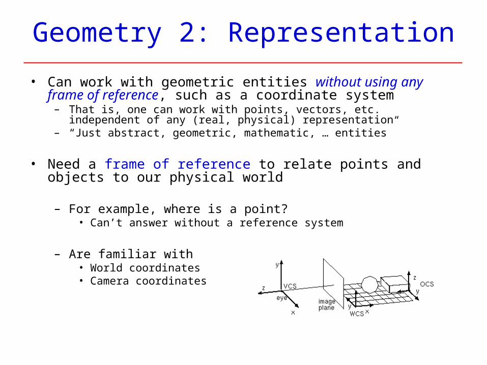
Geometry 2: Representation
• Can work with geometric entities without using any frame of reference, such as a coordinate system
– That is, one can work with points, vectors, etc. independent of any (real, physical) representation
– “Just abstract, geometric, mathematic, … entities”
• Need a frame of reference to relate points and objects to our physical world
– For example, where is a point? • Can’t answer without a reference system
– Are familiar with• World coordinates• Camera coordinates
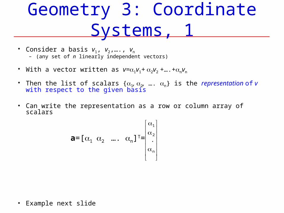
Geometry 3: Coordinate Systems, 1
• Consider a basis v1, v2,…., vn – (any set of n linearly independent vectors)
• With a vector written as v=1v1+ 2v2 +….+nvn
• Then the list of scalars {1, 2, …. n} is the representation of v with respect to the given basis
• Can write the representation as a row or column array of scalars
• Example next slide
a=[1 2 …. n]T=
n
2
1
.
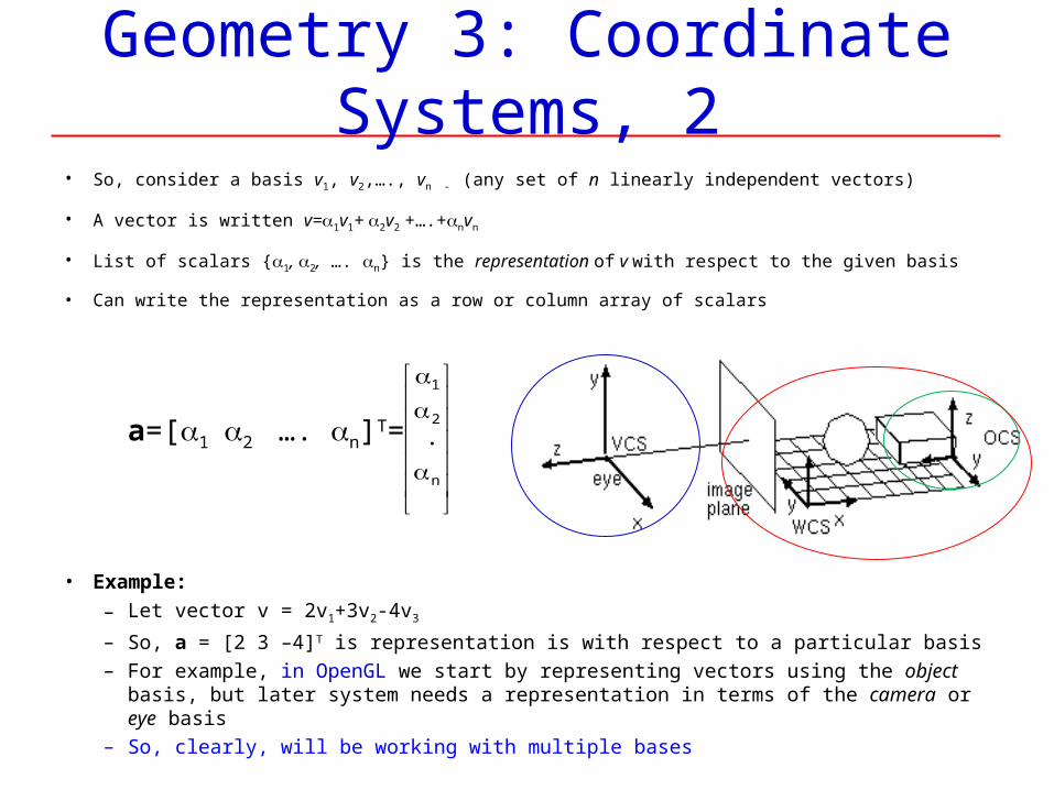
Geometry 3: Coordinate Systems, 2
• So, consider a basis v1, v2,…., vn - (any set of n linearly independent vectors)
• A vector is written v=1v1+ 2v2 +….+nvn
• List of scalars {1, 2, …. n} is the representation of v with respect to the given basis
• Can write the representation as a row or column array of scalars
• Example:
– Let vector v = 2v1+3v2-4v3
– So, a = [2 3 –4]T is representation is with respect to a particular basis– For example, in OpenGL we start by representing vectors using the object basis,
but later system needs a representation in terms of the camera or eye basis– So, clearly, will be working with multiple bases
a=[1 2 …. n]T=
n
2
1
.
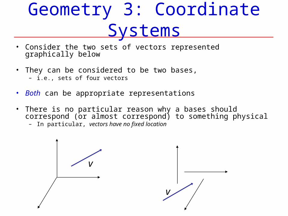
Geometry 3: Coordinate Systems• Consider the two sets of vectors represented graphically below
• They can be considered to be two bases, – i.e., sets of four vectors
• Both can be appropriate representations
• There is no particular reason why a bases should correspond (or almost correspond) to something physical
– In particular, vectors have no fixed location
v
v
Geometry 3: FramesNow, we slow down
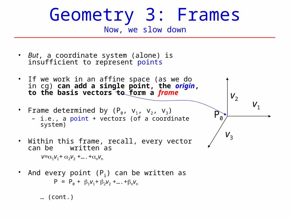
• But, a coordinate system (alone) is insufficient to represent points
• If we work in an affine space (as we do in cg) can add a single point, the origin, to the basis vectors to form a frame
• Frame determined by (P0, v1, v2, v3)– i.e., a point + vectors (of a coordinate system)
• Within this frame, recall, every vector can be written as
v=1v1+ 2v2 +….+nvn
• And every point (Pi) can be written as P = P0 + 1v1+ 2v2 +….+nvn
… (cont.)
P0
v1
v2
v3
Geometry 3: Frames & Homogeneous Coordinates
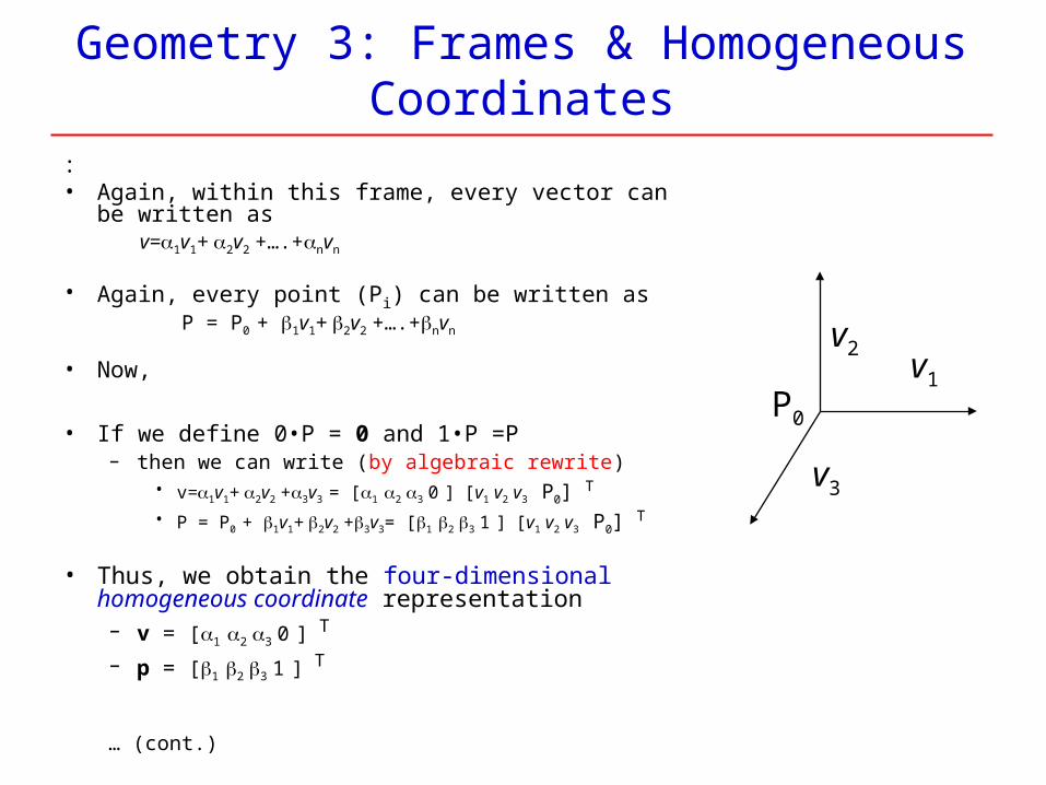
:• Again, within this frame, every vector can be written
as v=1v1+ 2v2 +….+nvn
• Again, every point (Pi) can be written as P = P0 + 1v1+ 2v2 +….+nvn
• Now,
• If we define 0•P = 0 and 1•P =P – then we can write (by algebraic rewrite)
• v=1v1+ 2v2 +3v3 = [1 2 3 0 ] [v1 v2 v3 P0]
T
• P = P0 + 1v1+ 2v2 +3v3= [1 2 3 1 ] [v1 v2 v3 P0]
T
• Thus, we obtain the four-dimensional homogeneous coordinate representation
– v = [1 2 3 0 ] T
– p = [1 2 3 1 ] T
… (cont.)
P0
v1
v2
v3
Geometry 3: Homogeneous Coordinates
:.• Again, thus we obtain the four-dimensional homogeneous coordinate
representation– v = [1 2 3 0 ]
T
– p = [1 2 3 1 ] T
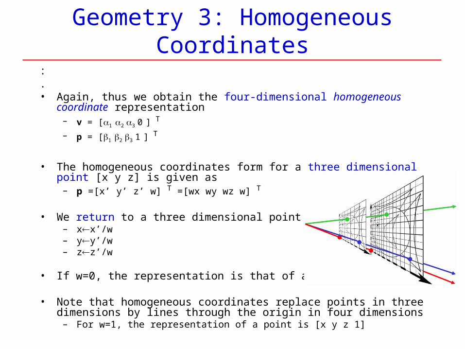
• The homogeneous coordinates form for a three dimensional point [x y z] is given as
– p =[x’ y’ z’ w] T =[wx wy wz w] T
• We return to a three dimensional point (for w0) by– xx’/w– yy’/w– zz’/w
• If w=0, the representation is that of a vector
• Note that homogeneous coordinates replace points in three dimensions by lines through the origin in four dimensions
– For w=1, the representation of a point is [x y z 1]
Geometry 3: Homogeneous Coordinates and CG
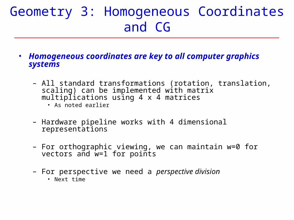
• Homogeneous coordinates are key to all computer graphics systems
– All standard transformations (rotation, translation, scaling) can be implemented with matrix multiplications using 4 x 4 matrices
• As noted earlier
– Hardware pipeline works with 4 dimensional representations
– For orthographic viewing, we can maintain w=0 for vectors and w=1 for points
– For perspective we need a perspective division• Next time
Geometry 3: Change of Coordinate SystemsGrand Finale
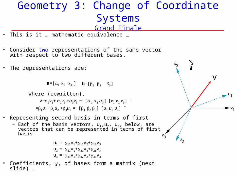
• This is it … mathematic equivalence …
• Consider two representations of the same vector with respect to two different bases.
• The representations are:
• Representing second basis in terms of first – Each of the basis vectors, u1,u2, u3, below, are vectors
that can be represented in terms of first basis
• Coefficients, , of bases form a matrix (next slide) …
u1 = 11v1+12v2+13v3
u2 = 21v1+22v2+23v3
u3 = 31v1+32v2+33v3
va=[1 2 3 ] b=[1 2 3]
Where (rewritten), v=1v1+ 2v2 +3v3 = [1 2 3] [v1 v2 v3] T
=1u1+ 2u2 +3u3 = [1 2 3] [u1 u2 u3] T
G 3: Change of Coord. System - Matrix Form
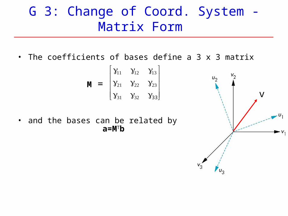
• The coefficients of bases define a 3 x 3 matrix
• and the bases can be related by
a=MTb
33
M =v
Geometry 3: Change of Frames
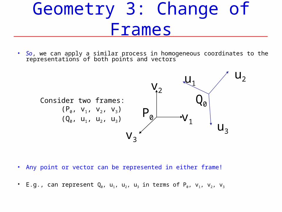
• So, we can apply a similar process in homogeneous coordinates to the representations of both points and vectors
• Any point or vector can be represented in either frame!
• E.g., can represent Q0, u1, u2, u3 in terms of P0, v1, v2, v3
Consider two frames: (P0, v1, v2, v3) (Q0, u1, u2, u3)
P0 v1
v2
v3
Q0
u1u2
u3
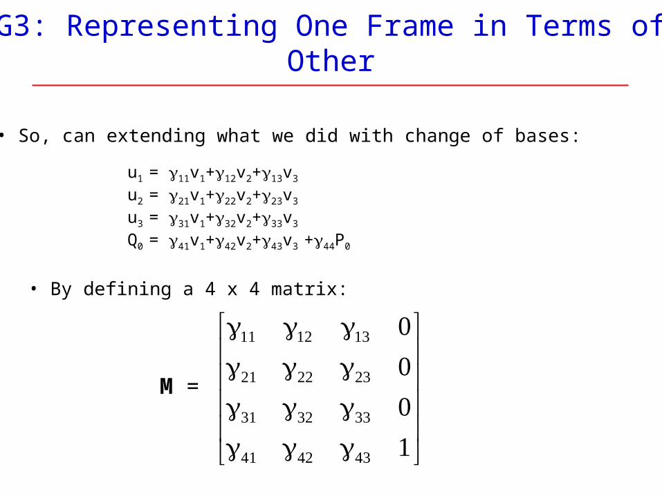
G3: Representing One Frame in Terms of Other
u1 = 11v1+12v2+13v3
u2 = 21v1+22v2+23v3
u3 = 31v1+32v2+33v3
Q0 = 41v1+42v2+43v3 +44P0
• So, can extending what we did with change of bases:
• By defining a 4 x 4 matrix:
M =
G 3: Working with Representations
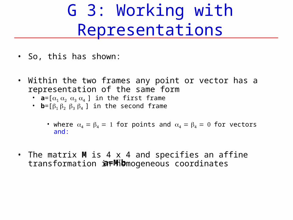
• So, this has shown:
• Within the two frames any point or vector has a representation of the same form
• a=[1 2 3 4 ] in the first frame• b=[1 2 3 4 ] in the second frame
• where 4 4 for points and 4 4 for vectors and:
• The matrix M is 4 x 4 and specifies an affine transformation in homogeneous coordinates
a=MTb
Geometry 3: Affine TransformationsConclusion
• Every linear transformation is equivalent to a change in frames
• Every affine transformation preserves lines
• However, an affine transformation has only 12 degrees of freedom because 4 of the elements in the matrix are fixed and are a subset of all possible 4 x 4 linear transformations
OGL: World and Camera Frames
OGL: World and Camera Frames
• When we work with representations, we work with n-tuples or arrays of scalars
• Changes in frame are then defined by 4 x 4 matrices– And this is what we saw coming to this the other way around
• In OpenGL, base frame that we start with is the world frame
• Eventually, we represent entities in the camera frame by changing the world representation using the model-view matrix
• Initially, these frames are the same (M=I)
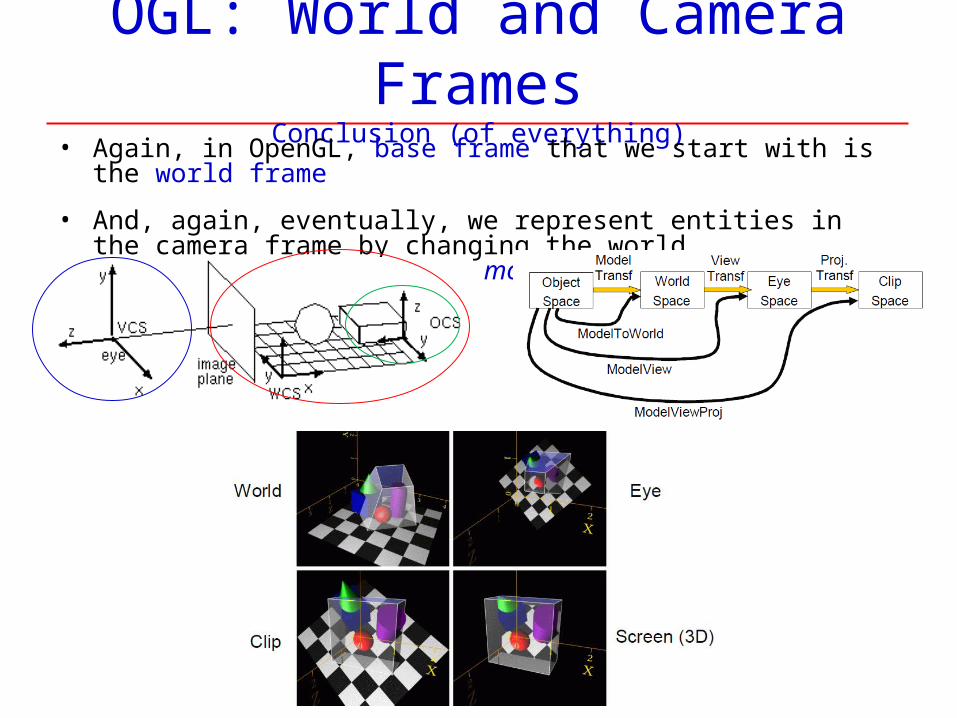
OGL: World and Camera FramesConclusion (of everything)
• Again, in OpenGL, base frame that we start with is the world frame
• And, again, eventually, we represent entities in the camera frame by changing the world representation using the model-view matrix
End
• .
Homework 4Animating Object Display and User Directed Camera Movement
• Have a look at Angel programs at web site
Homework 4Animating Object Display and User Directed Camera Movement
• Create a program to allow users to animate display and “fly around” the objects created.
– This program builds on the functionality of your third program. Hopefully, no significant change to data structures and program structure will be necessary.
• This program should: – 1) Animate the initial display of objects, when a file is read– 2) Allow the user to position the camera so that the view on the display is like a
“fly around” of the objects.
• For extra credit, implement the two items from the last assignment
Homework 4Animating Object Display and User Directed Camera Movement
• 1) Animate the initial display of objects, when a file is read. – 3a) Allow the user to select a “fast” or “slow” animation and – 3b) whether objects are animated simultaneously or individually (see below).
• The animation should begin by drawing all objects at the center of the screen, when a file is read.
– Then, each figure should move to its former (saved) location. • Recall, y = mx + b. Use double buffering.
• The user can select at start up whether the movement of objects will be one at a time or simultaneously, i.e.,
– b1) each figure in turn might move from the center of the screen to its location, or– b2) all figures might move simultaneously toward their locations. – In the latter case there are a host of decisions to be made about how exactly to
do that, and, rather than specify all here, just make decisions and document them.
Homework 4Animating Object Display and User Directed Camera Movement
• 2) Allow the user to position the camera so that the view on the display is like a “fly around” of the objects.
– That is, the camera remains pointed at the origin (or some point), and its position is moved through user input.
– Using the elementary keyboard input scheme discussed in class and presented in Angel’s programming example is fine.
• • For extra credit, implement the two items from the last assignment,
if you haven’t done so already: – a) Allow the user to specify that all the polygons spin. Like Angel’s example. – b) Implement rubber banding, using xor as discussed, when the cursor is moved
to pick an object. The fixed point of the rubber band should be the center of the screen and the user should be able to turn on and off rubber banding by a menu.
– (more extra credit)
Homework 4Animating Object Display and User Directed Camera Movement
• Also for extra credit, allow the user more options for positioning and aiming the camera in addition to the functionality of 2) above,
– e.g., aim the camera at other positions than the origin, allow “tilting” of the camera by changing the up vector, etc.
– Having the camera “fly” by itself through some course would be interesting, as well.
– Of course, in essentially all applications mouse movement, often with button presses is used to position and aim the camera, and implementing this sort of interaction would also be an extra credit activity interesting to pursue.
• When complete, please upload to the class Blackboard site: – 1) a description (200-400 words … really, more) of what the program does – 2) a screen capture showing the display when three objects have been created,
3) source code and • This time, must be able to execute – will follow up, as needed
– 4) executable.
• Due two weeks – 3/10

Term Project 25% of Course Grade
Term Project25% of Course Grade
• The term programming project will consist of the design, implementation, documentation, and demonstration of a moderately complex computer graphics software system and will account for 25% of the final grade.
• The purpose of the project is to provide the student with an opportunity to explore the application of computer graphics in a domain of his or her choosing.
• It is genuinely intended to provide a platform for creativity, as well as workman like execution.
• The domain of the project can be in any area: from implementation of a computer graphics algorithm (or its extension) to games to visualization to ….
• There are many computer graphics student project titles available via the web, so look around, have a go at something that interests you, be creative, and enjoy. The project consists of the elements below.
Term Project Components
• Proposal / design, 10%
• Milestones, 5%
• Implementation, 50%
• Report / documentation, 10%
• Demonstration, 25%
Proposal / design, 10%
• A two page proposal (12 pt. font, single space, 1” margins) will outline the project and its motivation.
• Proposals must be approved by the instructor. • After submitting the proposal (2/26 12:00 noon or before),
preliminary feedback will be given within one day. • The feedback will be of the form: ok, ok with revisions/suggestions
delineated in the initial feedback, or “we should talk”, in which case arrangements for a conversation will be made such that the revisions can be completed by week’s end.
• Getting the proposal in early makes a lot of sense. Just talking about ideas over the first couple of weeks makes a lot of sense, too.
• Remember, the range of possibilities is large, and iteration with the instructor can facilitate development of a proposal that is both within the scope of the class and can be completed in the semester’s time frame.
Milestones, 5%
• Notwithstanding the difficulty in estimating software project time (made an order of magnitude harder by programming in an unfamiliar system), the proposal should include milestones for 4/2 that will include an executable be delivered to the instructor, as detailed in the next section.
• The milestones must be clear and stated as measureable elements.• This will likely require a design and implementation strategy that
creates a system that can be developed in stages in which there is some subset of final functionality available at each stage.
Implementation, 50%
• The system must make use of OpenGL for its computer graphics capabilities, and whatever else you would like for any window system and other functionality, e.g., Qt.
• In class, we will note the wide availability of code examples. By all means make use of them, but by no means take any credit, i.e., carefully document in the code the source of any code you have not written. Failure to do so will result in a grade reduced as a function of the amount of code not cited.
• The code itself should be reasonably well documented with respect to algorithms, structure, etc., sufficient that the instructor can make sense of it.
Implementation, 50% (cont.)
• At milestone date code and executable will be submitted in the same manner as homework and, as with homework, the assignment will not be accepted after the date on which it is due.
• Of course, it is possible and reasonable that the functionality described at the milestone will not be achieved. If that is the case, and appropriate effort can be documented, e.g., “tried this that and the other and here is the 1000 lines of code that did not work”, then no deduction in score will be made.
• This is a tricky one – my hope is that you would propose an ambitious project and we can manage risk appropriately. More in class.

Report / documentation, 10%
• On the night of the first demonstration (4/23) a five page summary of the project is to be turned in.
• The report should document your efforts and accomplishment in light of the proposal, as well as any difficulties, lessons learned, etc.

End