transfer lines paper studies -...
TRANSCRIPT

TRANSFER LINES – PAPER STUDIES
Wolfgang Bartmann
CAS, Erice, March 2017
Outline
• Introduction• What is a transfer line?
• Paper studies• Geometry – estimate of bend angles• Optics – estimate of quadrupole gradients and apertures• Error estimates and tolerances on fields
• Examples of using MADX for• Optics and survey matching• Achromats• Final focus matching• Error and correction studies
• Special cases in transfer lines• Particle tracking• Plane exchange• Tilt on a slope• Gantry matching• Dilution• Stray fields
1st hour
2nd hour
3rd hour

General beam transport
''''21'
2
2
x
x
SC
SC
x
x
x
xM
x
x
y
y
ss
1
2
n
i
n
1
21 MM
…moving from s1 to s2 through n elements, each with transfer matrix Mi
sincossin1cos1
sinsincos
22
12121
21
2111
2
21MTwiss parameterisation

Circular Machine
Circumference = L
• The solution is periodic
• Periodicity condition for one turn (closed ring) imposes 1=2, 1=2, D1=D2
• This condition uniquely determines (s), (s), (s), D(s) around the whole ring
QQQ
QQQ
L
2sin2cos2sin11
2sin2sin2cos2021 MMOne turn

Circular Machine
• Periodicity of the structure leads to regular motion
– Map single particle coordinates on each turn at any location
– Describes an ellipse in phase space, defined by one set of a and b values Matched Ellipse (for this location)
x
x’
2
max
1'
ax
ax max
Area = a
2
22
1
''2
xxxxa

Circular Machine
• For a location with matched ellipse (a, b), an injected beam of emittance e, characterised by a different ellipse (a*, b*) generates (via filamentation) a large
ellipse with the original a, b, but larger e
x
x’
After filamentation
,
, ,
, ,
x
x’
After filamentation
,
, ,
, ,
Matched ellipse determines beam shape
Turn 1 Turn 2
Turn 3 Turn n>>1
See V. Kain’slecture

Transfer line
sincossin1cos1
sinsincos
22
12121
21
2111
2
21M
'21'
2
2
x
x
x
xM
'
1
1
x
x
• No periodic condition exists
• The Twiss parameters are simply propagated from beginning to end of line
• At any point in line, (s) (s) are functions of 1 1
Single pass:
'
2
2
x
x

Transfer line
L0M
• On a single pass there is no regular motion
– Map single particle coordinates at entrance and exit.
– Infinite number of equally valid possible starting ellipses for single particle……transported to infinite number of final ellipses…
x
x’
x
x’
1, 1
1, 1
Transfer Line
2, 2
2, 2
'
2
2
x
x
'
1
1
x
x
Entry Exit
1500 2000 2500 30000
50
100
150
200
250
300
350
S [m]
Beta
X [
m]
Horizontal optics
Transfer Line
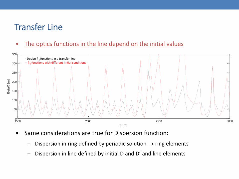
• The optics functions in the line depend on the initial values
• Same considerations are true for Dispersion function:
– Dispersion in ring defined by periodic solution ring elements
– Dispersion in line defined by initial D and D’ and line elements
- Design x functions in a transfer line x functions with different initial conditions
Transfer Line
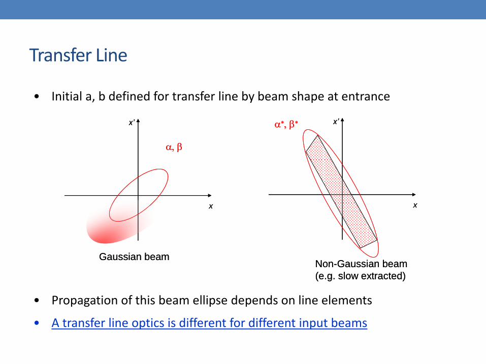
• Initial a, b defined for transfer line by beam shape at entrance
• Propagation of this beam ellipse depends on line elements
• A transfer line optics is different for different input beams
x
x’
,
x
x’,
Gaussian beamNon-Gaussian beam
(e.g. slow extracted)
x
x’
,
x
x’,
Gaussian beamNon-Gaussian beam
(e.g. slow extracted)
1500 2000 2500 30000
50
100
150
200
250
300
350
S [m]
Beta
X [
m]
Horizontal optics
Transfer Line
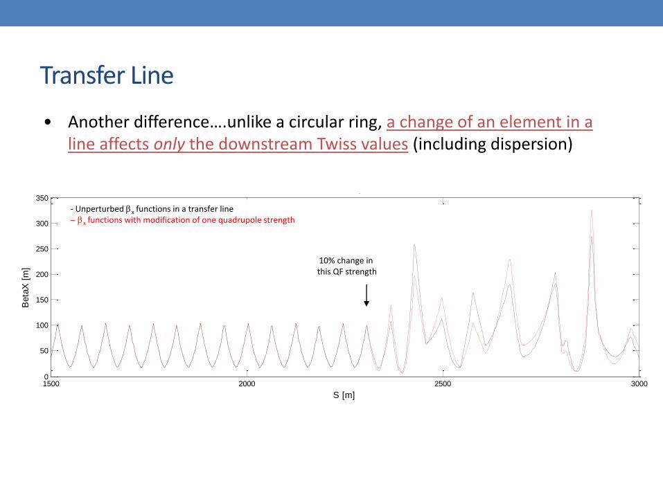
• Another difference….unlike a circular ring, a change of an element in a line affects only the downstream Twiss values (including dispersion)
10% change in this QF strength
- Unperturbed x functions in a transfer line x functions with modification of one quadrupole strength

Linking Machines
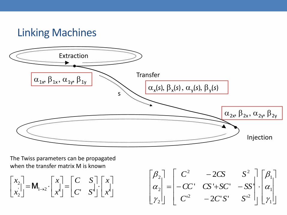
• Beams have to be transported from extraction of one machine to injection of next machine
– Trajectories must be matched, ideally in all 6 geometric degrees of freedom (x,y,z,theta,phi,psi)
• Other important constraints can include
– Minimum bend radius, maximum quadrupole gradient, magnet aperture, cost, geology
Linking Machines
1
1
1
22
22
2
2
2
'''2'
''''
2
SSCC
SSSCCSCC
SCSC
Extraction
Transfer
Injection
1x, 1x , 1y, 1yx(s), x(s) , y(s), y(s)
s
The Twiss parameters can be propagated when the transfer matrix M is known
''''21'
2
2
x
x
SC
SC
x
x
x
xM
2x, 2x , 2y, 2y
Linking Machines
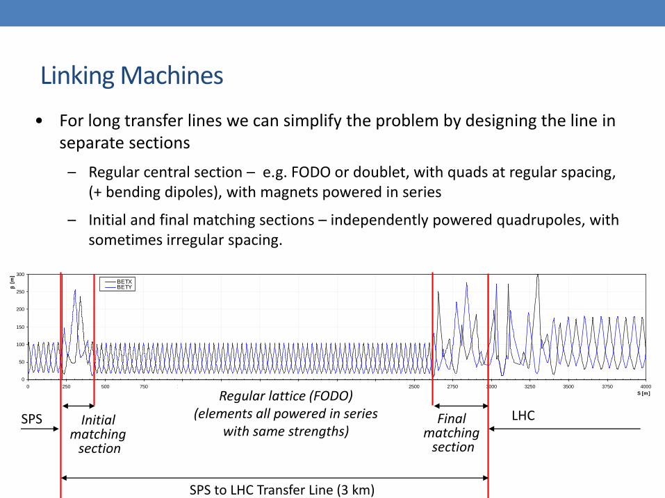
• For long transfer lines we can simplify the problem by designing the line in separate sections
– Regular central section – e.g. FODO or doublet, with quads at regular spacing, (+ bending dipoles), with magnets powered in series
– Initial and final matching sections – independently powered quadrupoles, with sometimes irregular spacing.
0
50
100
150
200
250
300
0 250 500 750 1000 1250 1500 1750 2000 2250 2500 2750 3000 3250 3500 3750 4000
S [m]
[
m]
BETXBETY
SPS LHC
Regular lattice (FODO)(elements all powered in series
with same strengths)Final
matching section
SPS to LHC Transfer Line (3 km)
Initial matching
section

Outline
• Introduction• What is a transfer line?
• Paper studies• Geometry – estimate of bend angles• Optics – estimate of quadrupole gradients and apertures• Error estimates and tolerances on fields
• Examples of using MADX for• Optics and survey matching• Achromats• Final focus matching• Error and correction studies
• Special cases in transfer lines• Particle tracking• Plane exchange• Tilt on a slope• Dilution• Stray fields
1st hour
2nd hour
3rd hour
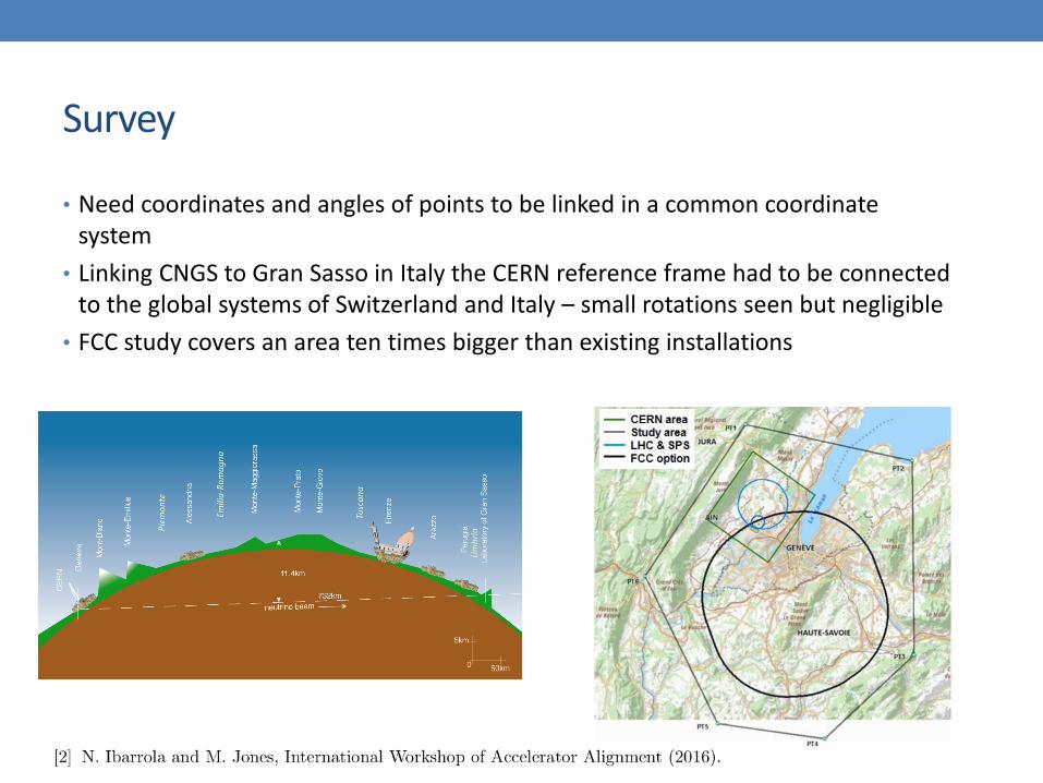
Survey
• Need coordinates and angles of points to be linked in a common coordinate system
• Linking CNGS to Gran Sasso in Italy the CERN reference frame had to be connected to the global systems of Switzerland and Italy – small rotations seen but negligible
• FCC study covers an area ten times bigger than existing installations
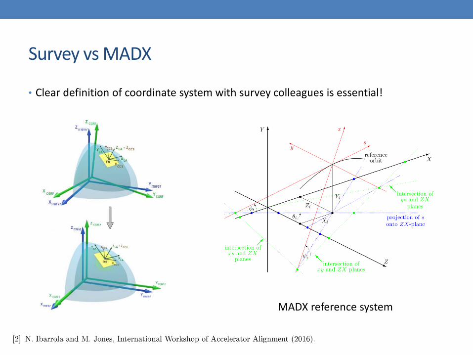
Survey vs MADX
• Clear definition of coordinate system with survey colleagues is essential!
MADX reference system

Bending fields
• Magnetic and electric rigidity:
• Deflection angle:
A … atomic mass numbern … charge statep … average momentum per nucleon
T … average kinetic energy per nucleon

Where is the limit between electric and magnetic?
• Electric devices are limited by the applied voltage – one can assume several 10s of kV as limit for reasonable accelerator apertures
• Magnets are limited by the field quality at low fields• Strong dependence on material properties
• Remnant fields become important
• Measuring the field becomes a challenge
• Example• 100 keV antiprotons
• Electrostatic quadrupoles with 60 mm diameter require applied voltages of below 10 kV
• Electrostatic bends of up to 30 kV

If you are in the energy grey zone…how to choose between magnetic and electric?
• Cheap element production
• Cheap power supplies and cabling
• Mass-independent
• No hysteresis effects (easy operation)
• No power consumption – no cooling
• Transverse field shape easy to optimize
• Difficult to measure field shape –effective length
• Diagnosis of bad connections
• Inside vacuum• Large outgassing surface area
• Vulnerable to dirt inside vacuum
• Requires vacuum interlock for sparking and safety
• Repair requires opening the vacuum
• Limited choice of vacuum and bake-out compatible insulators
Pros and cons of electrostatic beam lines:
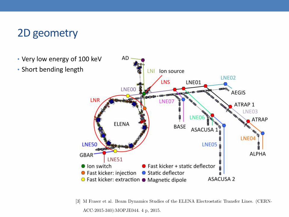
2D geometry
• Very low energy of 100 keV
• Short bending length

2D geometry
• 36 cm vertical height difference over several m
• 1-2 GeV

More complex 3D geometry
Bending over the full TL length - assume reasonable dipole filling factor ~70%
Linda Stoel
Several 100 m vertical, several km length, 3.3 TeV…distributed bending

Bending field limits
• So far we considered the bending fields in transfer lines limited solely by hardware
• A few 10 kV on electrostatic devices to avoid sparking
• 2 T for normal conducting magnets
• Something like existing LHC dipole reach 9-9.5 T for superconducting magnets
• But is there anything else which might limit the bending field?

Lorentz Stripping
• Transfer of H- ions
• Extra electron binding energy is 0.755 eV
• A moving ion sees the magnetic field in its rest frame – Lorentz transform gives electric field as
𝐸𝑀𝑉
𝑐𝑚= 3.197 ∙ 𝑝[
𝐺𝑒𝑉
𝑐] ∙ 𝐵[𝑇]
• Lifetime
𝜏 =𝐴
𝐸𝑒(
𝐶
𝐸) 𝐴 = 7.96 ∙ 10−14 s MV/cm, 𝐶 = 42.56 MV/cm

Example of PS2
• 4 GeV injection
• Fractional loss below 1e-4 limits magnetic field to 0.13 T

Example of Fermilab Project-X
• Was considered as proton source with 8 GeV H- into recycler ring for neutrino program
• Usual power loss limit in lines of ~1W/m
• Activation was found to be not acceptable for 8 GeV ions
• Reduction to 0.05 W/m power loss to meet radioprotection requirements
• In this regime also other loss processes become relevant…

Black body radiation

Black body radiation

Rest gas stripping
• Power loss due to stripping on rest gas per length l
Beam energyand intensity
Gas density …fct of T, p
Example Fermilab Project X
• Loss rate from black body radiation at 300 K not acceptable
• Installing a cool beam screen (77 K)
• Reduces black body radiation by factor ~16
• Improves vacuum pumping (better than 1e-8 Torr)
• Lorentz stripping limits dipole fields to 0.05 T

Focussing structure
• Cell length optimised for dipole filling at extraction energy
• Can assume this as a good starting point for our transfer line
• For transfer lines often a 90 deg FODO structure is chosen • Good ratio of max/min in beta function
• Same aperture properties
• Provides good locations for trajectory correctors and instrumentation
• Good phase advance for injection/extraction and protection equipment
0
50
100
150
200
250
300
0 250 500 750 1000 1250 1500 1750 2000 2250 2500 2750 3000 3250 3500 3750 4000
S [m]
[
m]
BETXBETY
SPS LHCFinal matching
section
SPS to LHC Transfer Line (3 km)
Initial matching
section
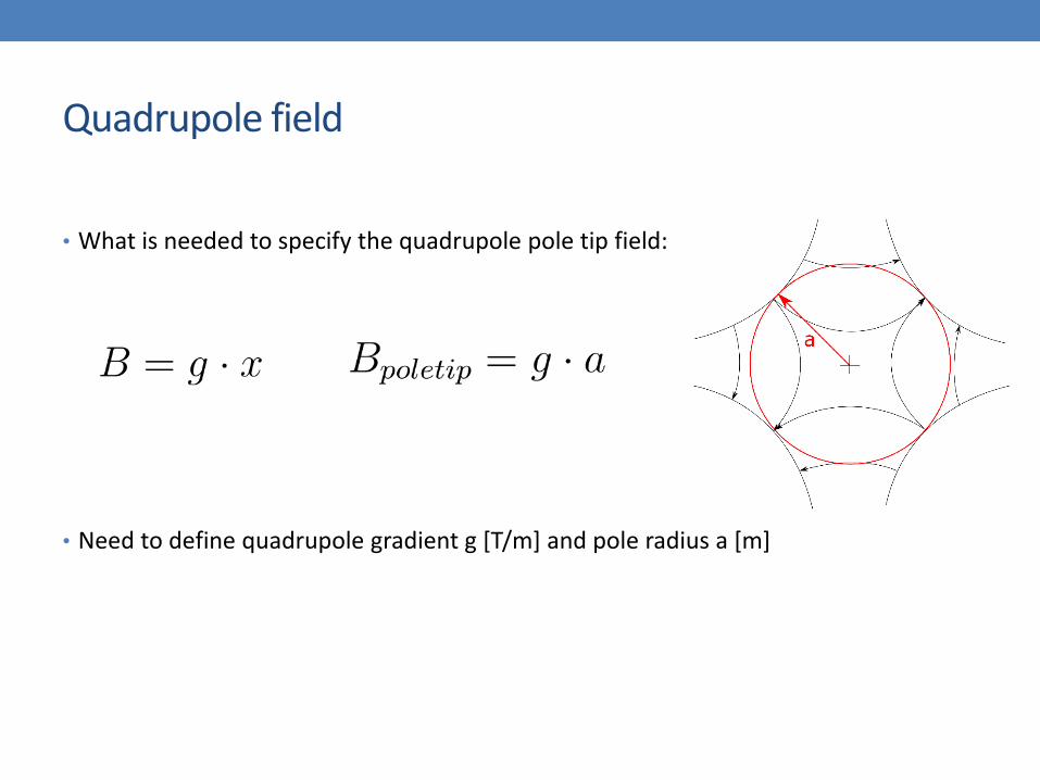
Quadrupole field
• What is needed to specify the quadrupole pole tip field:
• Need to define quadrupole gradient g [T/m] and pole radius a [m]

FODO cell
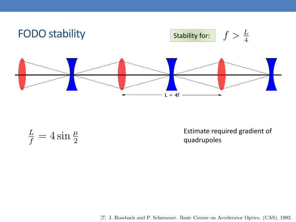
FODO stability
Estimate required gradient of quadrupoles
Stability for:
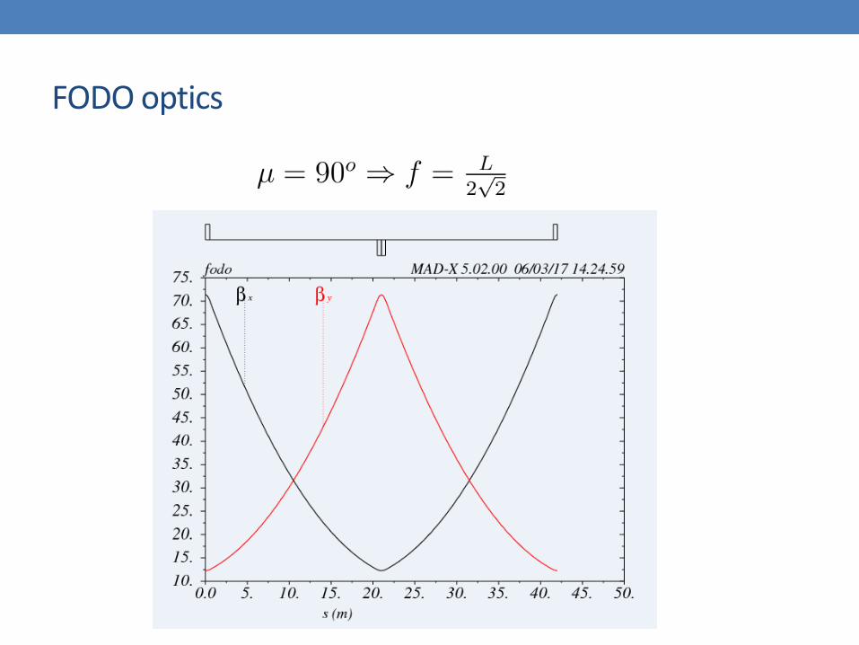
FODO optics

FODO stability
Estimate required gradient of quadrupoles
Use maximum betatron function to estimate beam size and pole tip field of quadrupoles
Apertures
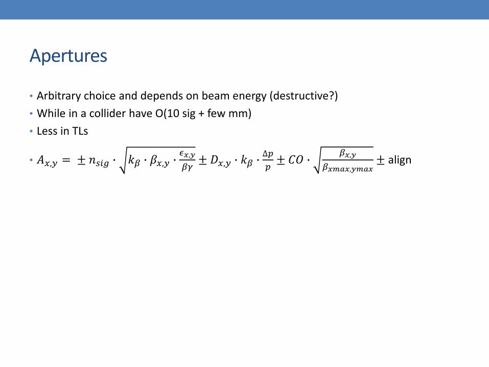
• Arbitrary choice and depends on beam energy (destructive?)
• While in a collider have O(10 sig + few mm)
• Less in TLs
• 𝐴𝑥,𝑦 = ± 𝑛𝑠𝑖𝑔 ∙ 𝑘𝛽 ∙ 𝛽𝑥,𝑦 ∙𝜖𝑥,𝑦
𝛽𝛾± 𝐷𝑥,𝑦 ∙ 𝑘𝛽 ∙
∆𝑝
𝑝± 𝐶𝑂 ∙
𝛽𝑥,𝑦
𝛽𝑥𝑚𝑎𝑥,𝑦𝑚𝑎𝑥± align
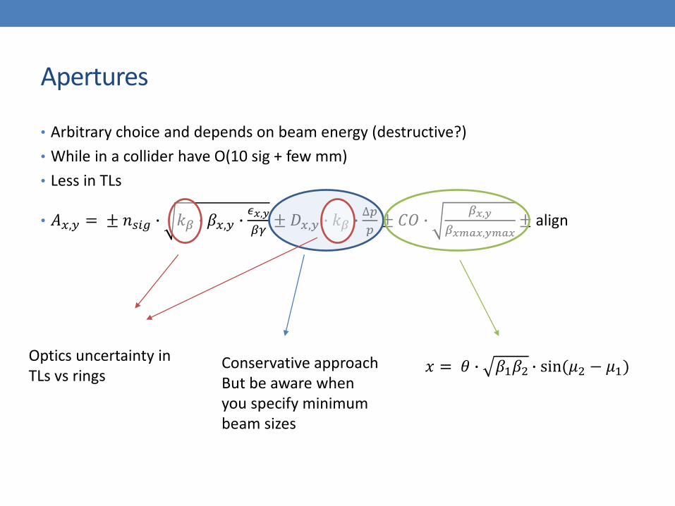
Apertures
• Arbitrary choice and depends on beam energy (destructive?)
• While in a collider have O(10 sig + few mm)
• Less in TLs
• 𝐴𝑥,𝑦 = ± 𝑛𝑠𝑖𝑔 ∙ 𝑘𝛽 ∙ 𝛽𝑥,𝑦 ∙𝜖𝑥,𝑦
𝛽𝛾± 𝐷𝑥,𝑦 ∙ 𝑘𝛽 ∙
∆𝑝
𝑝± 𝐶𝑂 ∙
𝛽𝑥,𝑦
𝛽𝑥𝑚𝑎𝑥,𝑦𝑚𝑎𝑥± align
Conservative approachBut be aware when you specify minimum beam sizes
𝑥 = 𝜃 ∙ 𝛽1𝛽2 ∙ sin(𝜇2 − 𝜇1)Optics uncertainty in TLs vs rings

Apertures
• Arbitrary choice and depends on beam energy (destructive?)
• While in a collider have O(10 sig + few mm)
• Less in TLs
• 𝐴𝑥,𝑦 = ± 𝑛𝑠𝑖𝑔 ∙ 𝑘𝛽 ∙ 𝛽𝑥,𝑦 ∙𝜖𝑥,𝑦
𝛽𝛾± 𝐷𝑥,𝑦 ∙ 𝑘𝛽 ∙
∆𝑝
𝑝± 𝐶𝑂 ∙
𝛽𝑥,𝑦
𝛽𝑥𝑚𝑎𝑥,𝑦𝑚𝑎𝑥± align
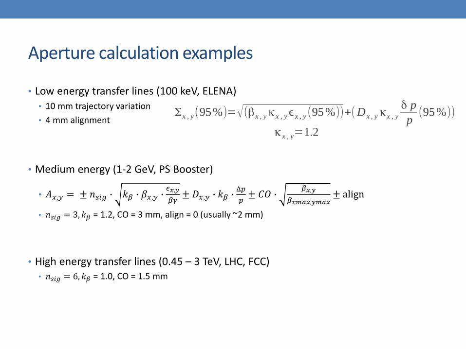
Aperture calculation examples
• Low energy transfer lines (100 keV, ELENA)• 10 mm trajectory variation
• 4 mm alignment
• Medium energy (1-2 GeV, PS Booster)
• 𝐴𝑥,𝑦 = ± 𝑛𝑠𝑖𝑔 ∙ 𝑘𝛽 ∙ 𝛽𝑥,𝑦 ∙𝜖𝑥,𝑦
𝛽𝛾± 𝐷𝑥,𝑦 ∙ 𝑘𝛽 ∙
∆𝑝
𝑝± 𝐶𝑂 ∙
𝛽𝑥,𝑦
𝛽𝑥𝑚𝑎𝑥,𝑦𝑚𝑎𝑥± align
• 𝑛𝑠𝑖𝑔 = 3, 𝑘𝛽 = 1.2, CO = 3 mm, align = 0 (usually ~2 mm)
• High energy transfer lines (0.45 – 3 TeV, LHC, FCC)• 𝑛𝑠𝑖𝑔 = 6, 𝑘𝛽 = 1.0, CO = 1.5 mm

First estimate of field error specification
• Impact of field errors on aperture requirements should be negligible
• Beam quality is the constraint – emittance growth
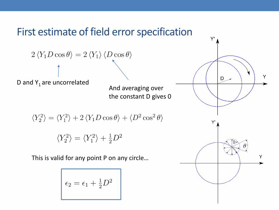
First estimate of field error specification
D and Y1 are uncorrelatedAnd averaging over the constant D gives 0
This is valid for any point P on any circle…

First estimate of field error specification
Magnet misalignment
Dipole field error
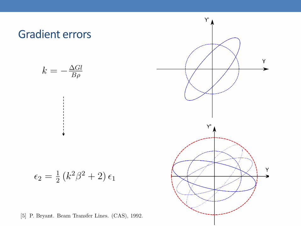
Gradient errors
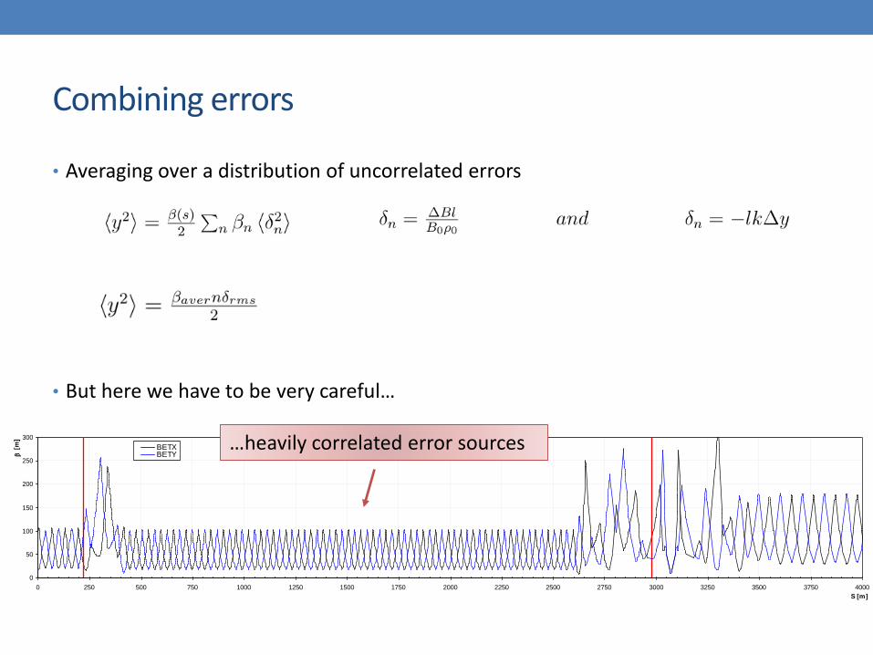
• Averaging over a distribution of uncorrelated errors
• But here we have to be very careful…
Combining errors
0
50
100
150
200
250
300
0 250 500 750 1000 1250 1500 1750 2000 2250 2500 2750 3000 3250 3500 3750 4000
S [m]
[
m]
BETXBETY
…heavily correlated error sources
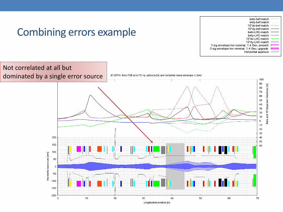
Combining errors example
Not correlated at all but dominated by a single error source
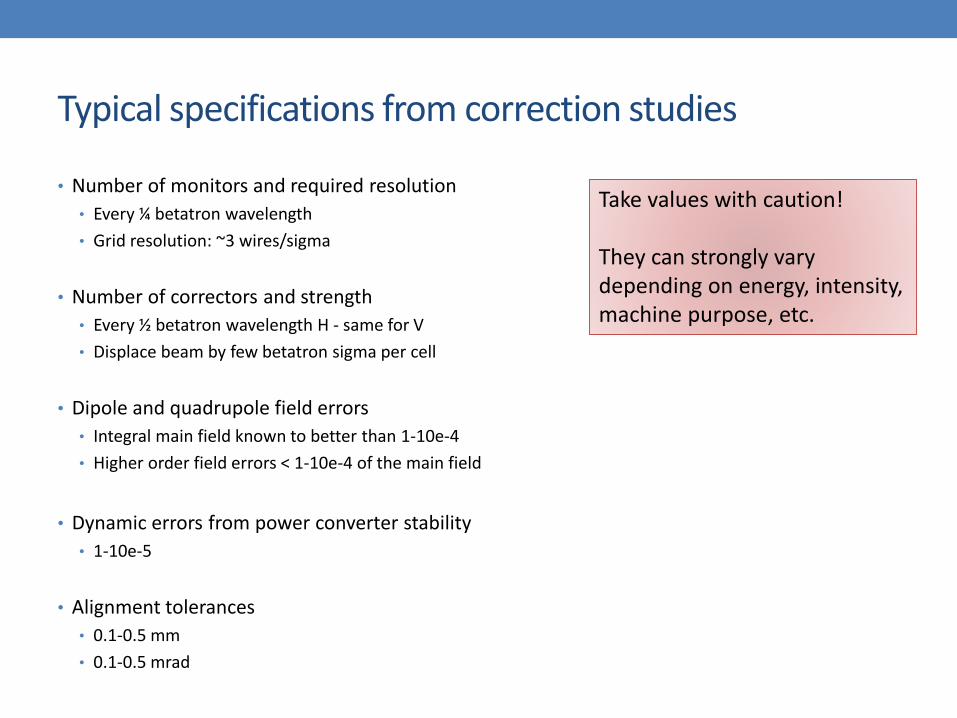
Typical specifications from correction studies
• Number of monitors and required resolution
• Every ¼ betatron wavelength
• Grid resolution: ~3 wires/sigma
• Number of correctors and strength
• Every ½ betatron wavelength H - same for V
• Displace beam by few betatron sigma per cell
• Dipole and quadrupole field errors
• Integral main field known to better than 1-10e-4
• Higher order field errors < 1-10e-4 of the main field
• Dynamic errors from power converter stability
• 1-10e-5
• Alignment tolerances
• 0.1-0.5 mm
• 0.1-0.5 mrad
Take values with caution!
They can strongly vary depending on energy, intensity, machine purpose, etc.
Summary
Before switching on a computer we can define for a transfer line:
• Number of dipoles and quadrupoles, correctors and monitors
• Dipole field and quadrupole pole tip field
• Aperture of magnets and beam instrumentation
• Rough estimate of required field quality and alignment accuracy

Wrap up
• Optics in a ring is defined by ring elements and periodicity – optics in a transfer line is dependent line elements and initial conditions
• Changes of the strength of a transfer line magnet affect only downstream optics
1500 2000 2500 30000
50
100
150
200
250
300
350
S [m]
Beta
X [
m]
Horizontal optics
L0M
x
x’
x
x’
1, 11, 1
Transfer Line
2, 2
2, 2
'
2
2
x
x
'
1
1
x
x
Entry Exit

Wrap up
• Geometry calculations require a set of coordinates in a common reference frame
• Bending fields are defined by geometry and the magnetic or electric rigidity:
• The choice between magnetic and electric depends mainly on the beam energy
• If you are in the grey zone, consider: field design and measurement, power consumption, vacuum, interlocking
• For the estimates of bending radii in lines remember to take into account the filling factor (~70%) and Lorentz-Stripping in case of H- ions

• Quadrupole gradients and apertures can be estimated in case of simple focussing structure like FODO cells
• Aperture specifications require safety factors for the optics and constant contributions for trajectory variations and alignment errors
• 𝐴𝑥,𝑦 = ± 𝑛𝑠𝑖𝑔 ∙ 𝑘𝛽 ∙ 𝛽𝑥,𝑦 ∙𝜖𝑥,𝑦
𝛽𝛾± 𝐷𝑥,𝑦 ∙ 𝑘𝛽 ∙
∆𝑝
𝑝± 𝐶𝑂 ∙
𝛽𝑥,𝑦
𝛽𝑥𝑚𝑎𝑥,𝑦𝑚𝑎𝑥± alignment
Wrap up
Stability
Defines beam size and quadrupole pole tip field

Magnet misalignment
Dipole field error
Wrap up
• Estimating tolerances from emittance growth:
• Dipole field and alignment:
• Gradient errors:
And many thanks to my colleagues for helpful input:
R. Baartman, D. Barna, M. Barnes, C. Bracco, P. Bryant, F. Burkart, V. Forte, M. Fraser, B. Goddard, C. Hessler, D. Johnson, V. Kain, T. Kramer, A. Lechner, J. Mertens, R. Ostojic, J. Schmidt, L. Stoel, C. Wiesner
Thank you for your attention