transcript 8-30-21 for iepr commissioner workshop on

DOCKETED Docket Number: 21-IEPR-05

Project Title: Natural Gas Outlook and Assessments

TN #: 240009

Document Title:

TRANSCRIPT 8-30-21 for IEPR COMMISSIONER

WORKSHOP ON NATURAL GAS MARKET AND DEMAND

FORECASTS

Description:

TRANSCRIPT 8.30.21 for IEPR COMMISSIONER

WORKSHOP ON NATURAL GAS MARKET AND DEMAND

FORECASTS

Filer: Raquel Kravitz

Organization: California Energy Commission

Submitter Role: Commission Staff

Submission Date: 10/7/2021 4:56:34 PM

Docketed Date: 10/7/2021

1

CALIFORNIA REPORTING, LLC

229 Napa Street, Rodeo, California 94572 (510) 224-4476

STATE of CALIFORNIA

CALIFORNIA ENERGY COMMISSION

STAFF WORKSHOP

In the Matter of: ) Docket No. 21-IEPR-05

)

)

2021 Integrated Energy Policy )

Report (2021 IEPR) )

) Re: Natural Gas Market

) and Demand Forecasts

______________________________ )

IEPR COMMISSIONER WORKSHOP

ON NATURAL GAS MARKET AND DEMAND FORECASTS

REMOTE-ACCESS ONLY

MONDAY, AUGUST 30, 2021

1:00 P.M.

Reported by: Elise Hicks

2



APPEARANCES

COMMISSIONERS PRESENT:

Commissioner J. Andrew McAllister, California Energy

Commission (CEC)

Commissioner Siva Gunda

Commissioner Karen Douglas

Commissioner Patty Monahan

Commissioner Houck, CPUC Commissioner

CEC STAFF PRESENT:

Heather Raitt, CEC

GAS FORECASTS AND LONG-TERM PLANNING OVERVIEW

Melissa Jones, Senior Energy Policy Specialist, CEC

NATURAL GAS MARKET PRESENTATIONS

Anthony Dixon, Lead Natural Gas Market Modeler, CEC

Ryan Ong, Natural Gas Market Modeler, CEC

UTILITY GAS DEMAND FORECAST/METHODOLOGIES PRESENTATIONS

Andrew Klingler, Senior Manager of Rate Architecture and Load

Forecast, PG&E

Todd Peterson, Principal, Energy Analysis and Insights, PG&E

Kurtis Kolnowski, Expert, Energy Analysis and Insights, PG&E

Amy Kouch, Analyst, Resource Forecasting, PG&E

Sharim Chaudhury, Manager, Cost Allocation and Rate Design, SoCalGas

Jeff Huang, Senior Resource Planner, SoCalGas

PUBLIC COMMENT

Mike Florio

1

3



INDEX

Page

1. Call to Order 4

2. Gas Forecasts and Long-Term Planning Overview 9

(Melissa Jones)

3. Natural Gas Market Presentations 22

(Anthony Dixon, Ryan Ong)

4. Utility Gas Demand Forecast/Methodologies 45

(Andrew Klingler, Todd Peterson,

Kurtis Kolnowski, Amy Kouch,

Sharim Chaudhury, Jeff Huang)

7. Public Comment 86

8. Adjournment 89

Reporter’s Certificate 90

Transcriber’s Certificate 91

1

4



P R O C E E D I N G S 1

August 30, 2021 1:01 P.M. 2

3

MS. RAITT: All right. Well, good afternoon, 4

everybody. Welcome to today’s IEPR 2021 Commissioner 5

Workshop on Natural Gas Market and Demand Forecasts. I’m 6

Heather Raitt, the Program Manager for Integrated Energy 7

Policy Reports. 8

This workshop is being held remotely consistent with 9

the Directive Order N08-21 to continue to help California 10

respond to, recover from, and mitigate the impacts of the 11

COVID-19 pandemic. The public can participate in the 12

workshop consistent with the direction in the Executive 13

Order. To follow along, the schedule and slide decks have 14

been docketed and are posted on the CEC’s website. Just go 15

to the 2020 -- 2021 IEPR webpage to find them. 16

All IEPR workshops are recorded and recording will be 17

linked to the Energy Commission’s website shortly following 18

the workshop and a written transcript will be available in 19

about a month. 20

Attendees have an opportunity to participate today in 21

a few different ways. For those joining through the Zoom 22

online platform, the Q&A feature is available for you to 23

submit questions. You may also upvote a question submitted 24

by someone else. Just click on the thumbs up icon to upvote. 25

5



Questions with the most upvote are moved to the top of the 1

queue. 2

There will be a few minutes near the end of the panel 3

to take questions, but likely will not have time to direct 4

all of the questions submitted. Alternatively, attendees may 5

make comments during the public comment period at the end of 6

the session. Written comments are also welcome and 7

instructions for doing so are in the workshop notice. 8

Written comments are due September 13. 9

And with that, I turn over to Commissioner Andrew 10

McAllister, the lead for 2021 IEPR. 11

Thank you. 12

COMMISSIONER MCALLISTER: Thank you, Heather. 13

Want to just again thank you. We had just a series 14

of very substantive workshops, rapid succession over the last 15

couple of weeks and I just want to express appreciation to 16

you and your staff for just keeping lots of plates spinning 17

and doing such an amazing job keeping the trains running down 18

the tracks because there are lots of them right now. 19

And no more important than this topic which is part 20

of our forecasting track and Commissioner Gunda leads this 21

effort. So I will only speak briefly here and leave the lion 22

share of the time for opening comments to him. But just, you 23

know, I have overseen this in the past, the forecasting, and 24

worked with Mr. Gunda on this for a number of years now. And 25

6



it is really just -- and before that with Chair Weisenmiller. 1

And it’s just the bread and butter of the Commission. It’s 2

one of the reasons the Commission was formed and it is no -- 3

in all the history of the Energy Commission, I think probably 4

we’re at a point where the forecasts are both more important 5

than they’ve even been and more intertwined between electric 6

and gas than they’ve ever been. 7

And this is a function of the time we’re living in 8

and the goals that we have. And really making sure that 9

we’re, I think, being situationally aware and that we’re 10

really looking at these issues from all the analytical 11

perspectives that might apply and with historical perspective 12

and with the sort of real time learning that we’re doing as a 13

state. And certainly trying to respond to the imperative of 14

reliability and health and safety and equity and just any 15

number, and decarbonization obviously. 16

So with so many -- not competing, so many 17

complementary goals here. We have to get them all right. So 18

the stakes are high on this and I know that we have a really 19

robust staff and very deep bench, really quality 20

professionals, the best there are, doing those analyses and 21

collecting all the information they need to underpin it. So 22

I’m just glad to be here today doing this and taking sort of 23

the next step in the gas demand forecasts. 24

So I would like to just wrap it up there and express 25

7



my appreciation to all the staff that’s been working on this, 1

and EID and then the IEPR team. 2

So over to you, Commissioner Gunda. 3

COMMISSIONER GUNDA: Thank you, Commissioner 4

McAllister. I mean, I would yield all my time to you, as you 5

know. You set the stage always so thoughtfully and then the 6

experience that you carry in these areas. Again, I always 7

like to say this, know it’s a pleasure to share the dais with 8

you now, this has been my mentor for several years, and now 9

as a colleague. 10

So with that, I really want to start with thanking 11

Heather and her incredible IEPR team. As usual, I’m really 12

looking forward to the meeting today, to the workshop today. 13

In interest of time, given that we have, you know, 14

some of the panelists need -- have tight deadlines here, are 15

hard stops. I do want to keep my comments brief. Just want 16

to invoke one specific thing that Commissioner McAllister 17

just mentioned which is that forecasting is a core 18

responsibility of the Energy Commission. And, you know, for 19

the last several years, we spend a lot more time as a 20

Commission going through the vetting of our electricity 21

demand forecasts given its importance in the IEPR, 22

transmission funding, and such. And for a long time, the 23

natural gas forecasts has been on kind of an equal of being 24

kind of a study -- study state. 25

8



But given the importance of the rapid climate goals 1

that we have in terms of electrification, it is important to 2

update and objectives analysis out there that provides, you 3

know, the forecast for natural gas. That could be another 4

data point as the industry double up their own forecast. So 5

I’m incredibly thankful for our natural gas team to 6

reinvigorating the process of the natural gas forecast, both 7

in the short term but also the broader long-term planning 8

scenarios. So it really helps the state with some critical 9

policy decisions and similar to how we do it on the Energy 10

Electricity Demand Forecast, I hope will create a robust 11

stakeholder process where we collectively generate a demand 12

forecast that we all feel comfortable as we pursue the long-13

term transition to a carbon neutrality and a zero carbon 14

California that is clean and reliable and affordable. 15

So with that, I am, you know, incredibly proud of the 16

work that our gas team is doing, Melissa Jones, Jennifer 17

Compagna, and A.J., Jason, everybody who’s going to speak 18

today. Thank you all for your incredible work. 19

With that, I’ll pass it on to Heather to commence the 20

very first presentation here unless we have any other 21

commissioners. 22

MS. RAITT: I don’t think we’ve had any commissioners 23

join yet, but. So thank you, Commissioner. 24

This is Heather. I’ll go ahead and get it started. 25

9



So our first presentation is from Melissa Jones, who is the 1

Senior Energy Policy Specialist in the Energy Commission’s 2

Assessment Division. And she’s going to give us an overview 3

of the day. 4

So thank you, Melissa. Go ahead. 5

MS. JONES: Thanks. Good afternoon, everyone. I am 6

Melissa Jones and I am first been a principal for both 7

electricity and natural gas issues with the Energy 8

Commission’s Assessment Division. 9

The goal of today’s workshop in the scoping order for 10

the 2021 IEPR, we identified the two primary issues for the 11

gas track. The situational awareness as a merging topic for 12

natural gas system planning. And then refinement and 13

development of critical analytical product that will be 14

necessary for gas planning in the state. 15

Today’s workshop is going to focus on gas market and 16

demand forecast topics. I will present an overview of 17

historic gas prices, rates, demands, and talk about forecast 18

improvements that we’re planning to make. Anthony Dixon, AJ, 19

will be providing an overview of our natural gas price and 20

rates forecast. And Ryan Ong, who is our newest member, will 21

be talking about the burner tip price forecast and electric 22

generation in the west. And then to cap off the afternoon, 23

the two gas utilities will be presenting their gas demand 24

forecasts and we’re looking forward to that. 25

10



I should also mention that the -- that we’ve had a 1

number of workshops on natural gas. We have three more topics 2

that are going to be viewed in workshop. Tomorrow we’re 3

having a workshop on renewable natural gas, and then later in 4

the process, December timeframe, we will be talking about 5

long-term demand scenarios and the gas demand forecast. 6

So the CEC presents forecasts. We do forecasting 7

assessments under the Warren Alquist Act which directs us to 8

forecast natural gas demands, supply, transportation, price, 9

rates, reliability, and efficiency. And we do this to 10

identify impacts on public health and safety, the economy, 11

energy diversity, resources, and the environment. And the 12

other thing the Energy Commission is charged with is to 13

identify emerging trends and impending or potential problems 14

or uncertainties in the electricity and natural gas markets 15

and in the industry as well. 16

Next slide, please. 17

So the Energy Commission’s forecast is used -- our 18

numerous forecasts are used in a number of different areas. 19

The forecasts feed into the California Energy Demand 20

Forecast, our natural gas price fits into that. Our natural 21

gas prices and demand also are inputs into the CEC’s PLEXOS 22

modeling for production cost modeling of the electricity 23

system. The CPUC uses price -- our prices in integrated 24

resource planning. The CAISO uses some of forecast in 25

11



transmission planning. WECC uses some of our forecast in 1

production cost modeling and in their policy and planning. 2

The Northwest Power and Conservation Council uses our 3

forecasting in policy and planning. And then the California 4

Gas Report, some of the utilities use our price forecasts as 5

an input to their forecasting activity. 6


This year we have focused on a number of improvements 8

in the gas forecasts. This is to follow up on 9

recommendations made in the 2019 IEPR for us to expand our 10

analytical capabilities. The CEC develops its commodity 11

price, gas price, using a North American Gas Market model 12

called NAMGas which captures the entire North American gas 13

market which is a continent-wide market. The CEC made a 14

major effort this time to expand the model from an annual 15

model to a monthly forecast. This allows us to better 16

capture seasonality and demand changes. 17

The CEC is using a new model that was developed by 18

Aspen. Katie Elder developed a model to forecast rates so we 19

can better incorporate revenue requirements and other factors 20

in our rate forecasts. 21

We’ve also made a number of improvements to the 22

Burner Tip Price forecast. And the Burner Tip Price is the 23

price that is used in PLEXOS as a proxy for natural gas costs 24

or natural gas prices. We developed a model that better 25

12



reflects price formation in the gas market. We realigned the 1

transportation rate from what used to be called proxy hubs 2

which were places that were near where power plants were 3

located. But they weren’t actual market hubs, meaning that 4

they weren’t liquid training points so we’ve reoriented that 5

model to now reflect actual market hubs. 6

And then we have gone through a process of 7

identifying improvements that will be needed to gas demand 8

forecasts to facilitate long-term planning. I’ll also be 9

talking about that. 10

I should say that in the IEPR, electricity issues are 11

usually front and center. We’re trying to put more emphasis 12

on natural gas and so part of what we’re doing in these 13

overview presentations is trying to familiarize people with 14

natural gas issues, those who aren’t familiar with it. 15


So in terms of gas supply trends, California gets 17

about 90 percent of its gas from out of state from supplies 18

that is 1,000 miles or more away from the state. Of that 90 19

percent, about 20 percent of it comes from Alberta, Canada 20

and it comes into California via Gas Transmission Northwest 21

pipeline. We get about 30 percent of our supplies from 22

southern Wyoming via the Ruby pipeline and the Kern River 23

pipeline. We get 40 percent of our gas from the San Juan 24

Basin, that’s the northwest New Mexico area and that is 25

13



transported via El Paso Natural Gas and Transwestern 1

pipeline. And then we get about 10 percent from the Permian 2

Basin which is both west Texas and southeast New Mexico 3

areas. And that also comes in via El Paso and Transwestern 4

pipeline. The other 10 percent of our supplies comes from 5

in-state production and that production has been slowly 6

declining since the 1980s and it’s anticipated to continue to 7

decline. 8


Oh, I should say one more thing. So PG&E generally 10

is more reliant on Canadian gas and SoCalGas relies more on 11

Rockies and San Juan gas. 12

Next slide, please. Gas prices. 13

So this graph shows volume weight rated Citygate 14

prices, average annual prices. And what you can see from 15

this is that California’s prices have tracked of the U.S. and 16

it’s actually been lower except during the 2001 -- 2000-2001 17

energy crisis. They’re fairly close to the U.S. I think 18

there’s an impression that California pays more for gas but 19

this is the situation. And what you can see here is that 20

since -- from the 1980s to about 2000, we had low fairly 21

stable gas prices in the state. 22

Starting in 2000 with the energy crisis, we had a big 23

peak in gas prices. FERC [Federal Energy Regulatory 24

Commission] investigated the market at that time and 25

14



discovered that there had been widespread market manipulation 1

which was the source of most of the price increases. And 2

California did recover about a billion dollars from gas 3

companies for this market manipulation. So gas prices 4

settled down a little bit after the crises and then in 2004, 5

they started to rapidly increase again. And by 2006, they 6

are very high. The peak was actually in 2010. And the reason 7

for this large increase in prices was basically competition 8

for what were declining production from traditional supply 9

basins. 10

At the time, we were looking at gas prices in the 14 11

to $20 range and so LNG imports became the focus of the 12

natural gas market in the United States. Numerous facilities 13

were constructed on the Gulf Coast and on the East Coast. 14

There were some that were purposed to be built up the 15

California coast, however, none of those moved forward. But 16

Sempra did develop its Costal Azul an LNG facility in Mexico. 17

And then starting in about 2000, shale gas began 18

production. So there were very rapid increases in technology 19

development combining hydraulic factoring with horizontal 20

drilling which produced a lot of gas. Starting in 2000, 21

about one percent of the gas produced in the United States 22

was from fracking. By 2010, it was over 20 percent and the 23

Energy Information Administration [EIA] predicts that by 24

2035, shale gas will constitute about 46 percent of all gas 25

15



produced in the United States. And since 1984 when we were 1

on that importer, we have now have moved to an exporter of 2

gas. 3

And then we saw that Citygate prices, you know, were 4

quite a bit lower, but we have seen some spikes in supply and 5

I can talk about those more as we move through. 6

And then, next slide, please. 7

So this slide shows a Henry Hub prices versus 8

California Border prices. And Henry Hub is a national 9

benchmark for pricing in the North American market. And what 10

you see here is there’s a very tight correlation between 11

Henry Hub and the Border prices in California. There was a 12

slight divergence starting in 2016. And at that point there 13

was excess Permian gas production which caused prices in the 14

San Juan basis to also drop which led to PG&E southern border 15

prices to fall. And then the SoCal Border prices did not 16

fall as much. And during that period we had the Aliso Canyon 17

leak and then we had pipeline outages which did contribute to 18

gas spikes in the state. 19


In terms of recent Citygate prices and rates in 21

California, the Citygate prices we also see a divergence 22

between Southern California and Northern California PG&E 23

Citygate. Largely this was due to pipeline outages. You can 24

see there’s a divergence in 2016 but the price didn’t really 25

16



diverge until -- and that was right when the leak had begun. 1

The prices didn’t really begin to diverge until about 2018 2

when we did have major pipeline outages on the SoCalGas 3

system. 4

In terms of rates, residential rates are the highest 5

rates and they have increased the most at about 4 percent per 6

year. And the reason was the prices or the rates are higher 7

for residential is because residential heating demand drive 8

the need for infrastructure and as such much more of the 9

costs of the natural gas system is allocated to residential 10

and commercial customers. You can see here that commercial 11

rates increased at about 2 percent. Industrial rates 12

increased at about 1.4 percent. And electric generation 13

rates actually decreased over that period, a little bit below 14

2 percent per year, except during that period when we had the 15

spike in Citygate prices in 2018. 16

We do think that with increasing electric generation 17

demand, at least daily draws on the natural gas systems that 18

due to the daily ramping to meet renewable integration needs 19

that that’s going to change the use of the gas system and it 20

may change the allocation of costs amongst these different 21

ratepayer classes. 22


So in terms of total gas by total energy consumption 24

in the state, natural gas actually counts for 28 percent of 25

17



our energy consumption. And in Btu equivalent, that’s more 1

gas -- that’s more gas that’s used in the state than gasoline 2

in the transportation sector. And I just pulled this slide 3

up a couple of days ago and kind of shocked to see that we 4

use as much natural gas as we do. And natural gas is a 5

dominant source for building, space, and water heating and 6

for industrial feedstock and fuel. And then it is the 7

dominant source on the electricity system. 8


So in terms of recent California gas demands, gas 10

demands have been declining since 2012, ’13. You’ll see 11

that there’s a lot of variation from year to year in gas 12

demands. Weather plays a big role in both residential and 13

commercial demands because it is for heating and it also 14

plays a big part in electric generation. And in addition to 15

weather during drought conditions, natural gas has been the 16

swing supply on the electricity system in California. We 17

have seen renewable integration needs increasing for electric 18

generation demands. Overall annual consumption of gas has 19

decreased, but these daily spikes are something that we’re 20

looking about -- looking towards and trying to plan around as 21

we move forward. 22

So I’m now going to shift, next slide, to the gas 23

demand forecast. 24

So this Energy Commission has long produced a gas 25

18



demand forecast as part of its California Energy Demand. 1

This is done every odd year. With the increased focus on 2

long-term gas planning, the Energy Commission does recognize 3

the need for new and different uses of our forecast and so we 4

have been looking at what kinds of improvements we can make. 5

In the 2021 IEPR, this is the first time that the Energy 6

Commission collected what are called forms and instructions 7

that contain the detailed inputs and assumptions for the 8

utilities’ demand forecasts, and they detailed the cost 9

information that is used to calculate the rate. We have done 10

this for a number of years on the electricity side and just 11

initiated this process on the gas side. 12

And then earlier this spring, we did engage our 13

expert panel which is composed of recognized experts in the 14

fields of energy forecasting and modeling to review our 15

forecast and make some recommendations about improvements. 16

Our expert panel is made up of these experts. We had James 17

McMann who’s the former head of Energy Analysis in LBNL 18

[Lawrence Berkeley National Laboratory] and he’s an energy 19

forecasting expert. 20

We have Hill Huntington who’s the Executive Director 21

of the Energy Modeling Forum from Stanford. And then we also 22

have Alan Sanstad who’s formerly with LBNL and currently with 23

the National Science Foundation Center for Robust Decision 24

Making, Modeling, and Climate. 25

19




So the expert panel gave us the Good Housekeeping 2

seal of approval for our forecast. They found the forecast 3

methodology is reasonable. They noted that the natural gas 4

demand forecast uses the same methodology as for electricity, 5

and they have previously reviewed our electricity forecast. 6

In addition, they have reviewed our transportation forecast. 7

They did note that the forecast should continue its 8

formal tie to the electricity forecast. They believed that 9

this is increasingly important especially with the 10

anticipated acceleration of electrification in residential 11

and commercial buildings in California. And then the other 12

major recommendation is that we needed to improve the 13

transparency of our forecast through stakeholder engagement. 14

We should do better model documentation and we should make 15

the model code more accessible and replicable so others 16

understand our forecast. 17


So they identified a number of near-term 19

improvements. The vetting and making the forecast results 20

transparent. We use what’s called the Demand Analysis 21

Working Group for our electricity forecast as well as the 22

transportation forecast. They recommended that we begin to 23

do that for our gas forecast. 24

They also recommended that we translate the 25

20



residential and commercial end-use models to modern platform. 1

They want us to incorporate the most recent surveys, the 2

Residential Appliance Survey and the Commercial End-Use 3

Survey into the forecast. And they suggest we re-examine the 4

econometric specifications as a natural gas model and re-5

estimate the equation that are routinely updated with new 6

data. They have recommended that we break out into separate 7

planning area. The gas deliveries by interstate, they go 8

directly to end-use customers in California in addition to 9

the two major gas utilities, PG&E and SoCalGas. 10

And then they have recommended greater collaboration 11

within our own assessment division so that we can discover 12

and correct data errors or misinterpretations, excuse me, and 13

be able to identify industry changes. 14


In terms of midterm improvements, they have 16

recommended that we develop approaches for forecasting under 17

different weather conditions. We do average conditions now 18

and we do an average annual demand forecast. 19

In the gas planning world, 1 in 10 condition, 1 in 20

35, and 1 in 90 are conditions that are used for basing 21

reliability standards so it’s important for us to have a 22

forecast that can be used in that arena. They’ve asked us to 23

craft usable, simple models to calculate natural gas 24

transportation rates that logically escalate and that with 25

21



expand over time and I mentioned earlier and will be talked 1

about more this afternoon. We do have our natural gas 2

transportation rate model and we have developed it so it can 3

expand in the future. 4

They have recommended that we continue to issue and 5

expand our forms and instructions to collect forecast 6

information in future years. They have recommend -- 7

COMMISSIONER GUNDA: Melissa. 8

MS. JONES: Yes. 9

COMMISSIONER GUNDA: Excuse me. I apologize to 10

interrupt you there. I think we are one slide behind. I 11

think we should move forward another slide. Yeah, thank you. 12

MS. JONES: Oh, sorry. I have my type in front of me 13

so I can’t see who is on the screen there. Thank you. 14

So in terms of midterm improvements, I mentioned that 15

forecasting under different weather conditions. We have 16

already started with the natural gas rates model. We’re 17

continually to do forms and instructions in the IEPRs. And 18

then they had suggested that we enhance our understanding of 19

industrial end uses, especially those that cannot be 20

electrified. 21

And then finally in terms of long-term gas 22

improvements, forecast improvements, they suggested that we 23

develop a forecast for hot, dry summer conditions. And on 24

our July 9th workshop, we represented some initial thoughts 25

22



about how to go about looking at summer demands. They’re 1

suggesting we develop more granular disaggregation in our 2

forecast so they can be used in hydraulic modeling of a gas 3

system, both geographically and hourly. This is especially 4

important to reflect to the electric generation burn on the 5

system. 6

We’ll need to capture climate change impact, 7

temperature, and occurrence of extreme events, both hot and 8

cold. They heat dome and polar vortex type event. Ensure 9

time in the process to iterate back and forth between price 10

and quantity. They suggest that we get daily and hourly gas 11

send out from utilities by customer class. And they 12

recommend that we continue corroboration with utilities in 13

developing more sophisticated forecasting methods 14

corresponding to the new and changing circumstances in the 15

gas market. 16

Next slide. 17

And with that, I think I’m done with my presentation. 18

Thank you for listening this afternoon. 19

MS. RAITT: Thank you so much, Melissa. 20

For our next speaker is Anthony Dixon, or A.J., and 21

he is the lead gas price modeler in the state through the 22

Energy Assessment Division. So Anthony will be covering the 23

CEC preliminary natural gas market results. 24

Go ahead. 25

23



MR. DIXON: Thank you. 1

MS. RAITT: Thank you. 2

MR. DIXON: All right. So, good afternoon, everyone 3

and Commissioners. I am Anthony Dixon or A.J. I am the lead 4

natural gas market forecaster, and I will be going over our 5

preliminary results for both the NAMGas [North American Gas-6

Trade Model] model and the new end-use rates and deliver 7

price modeling that we are working on. 8


So the NAMGas model we’ve been using for many years. 10

It’s a well vetted model using the MarketBuilder platform as 11

a general equilibrium model. Some of the updates to this 12

year’s model, of course, we always do North America demands 13

to reflect the current market conditions. We updated the 14

pipeline capacity throughout all of North America including 15

LNG infrastructure and a lot of new information on the 16

natural gas reserves and the costs. And we always vet these 17

out to the public and also internally and with Aspen 18

Environmental. 19


So the kind of the flow of what goes on with our 21

modeling efforts. The NAMGas model has three major inputs 22

that we work on. Those three are our resource model which 23

works with the capacities and costs associated with 24

production of natural gas throughout North America. We have 25

24



a small M model which is our demands throughout North 1

America. And there’s a caveat with that where we do not use 2

small m model to forecast demand in California and for power 3

gen and the WECC. There’s two other inside the Energy 4

Commission that does that modeling that we use their 5

information. And we do infrastructure research. 6

Off from the NAMGas model go directly to the PLEXOS, 7

or they go through a burner tip model and gas rates models 8

and then they get put into the production cost modeling. The 9

rates also go to a delivered rate model which go to our 10

demand forecast and then those go back to us. It’s kind of 11

an iterative process that we work out. 12


NAMGas model in a simplified version, it’s supply 14

basins that are connected to interstate and intrastate 15

pipelines which are connected to demand centers. And the 16

model basically calculates equilibrium across all time points 17

across all supply and demand at the same time. And it gives 18

us supply, it gives us production, it gives us flows, and it 19

gives us prices. 20


So some of the improvements and changes that we did 22

this year, we changed it from an annual model to a monthly 23

model. That gives us a model seasonal demand patterns that 24

we did not have before and also gives us the ability to 25

25



account for storage, which we never had before. And with so 1

many things dealing with storage, especially here in 2

California, that is a great addition that we’ll be able to 3

look into and see the effects on crisis. 4

We have a new resource allocation model. That’s our 5

supplies. Usually before we were given just the numbers by 6

consultants and that was what we took so now we actually 7

develop them ourselves. And we did a lot of streamlining 8

with the nodes inside the model to make it more real worldish 9

and also to streamline it and just make the model run a lot a 10

better. 11


With the corporation with IEPR, we do three common 13

cases, the high demand, mid-demand which is a business as 14

usual kind of case, and a low demand case. We will 15

hopefully, depending on time, be able to do some more 16

sensitivity analysis for the final run so we’ll be able to 17

look at a few more things throughout North America. 18

Next slide please. 19

So some of the key assumptions to start the model. 20

These are all kind of references to the model. The model 21

just takes these and when it does its balancing, it will 22

change demands, it’ll change prices, depending. Basically 23

for renewables, we make sure that we assume that in all cases 24

that California and all other states have met their RPS 25

26



targets that they have set. 1

We do a lot of research into these RPS targets for 2

all the states and including Canada and Mexico, if they have 3

any. We use a lot of EIA data, so their update are able to 4

pull North America data. We also, when it comes to data, we 5

also look at things like Canada. We deal their energy 6

information and also Mexico’s. 7

Next slide please. 8

And then this slide will show us the demand inputs 9

that we use for California. This is California specific. We 10

do not change these. Basically the numbers are a combination 11

of both the PLEXOS modeling and the California Energy demand 12

forecasts. We just take these numbers, we put them into the 13

model, we turn elasticities off so whatever they give us is 14

what the model will spit out as well. The only thing that 15

changes is the price. We don’t model these, we don’t change 16

them, we don’t do anything, we just take them from the other 17

forecasters. 18

We do do some extra work with the PLEXOS team where 19

we model a few times. Starting this year, this is the first 20

year we have been able to do this. We actually iterated 21

between each other five times, get our results to get a 22

little better equilibrium. 23


Then to continue on with some resources and their 25

27



costs, how we change them for each case. One of the big 1

things to kind of notice is the proved and potential 2

resources even in the mid-demand case and this kind of goes 3

into our results later on, is the fact that proved resources 4

keep growing even through we’re pulling record production. 5

Last year wasn’t record production, but we’ve been pulling 6

record production every year, usually, and proved in 7

potential resources keep going up. Our technology and what 8

gas we can get to keeps going up an they’re able not only to 9

produce more of it, but to produce more of it at lower and 10

lower costs. 11


So these are our U.S. demand projections that -- from 13

our modeling efforts by customer class and also overall. And 14

they do track very well with EIA’s latest annual energy 15

outlook. 16


So count some preliminary results directly from the 18

model. Henry Hub is one important that we really look at 19

because that is the national benchmark. And as Henry Hub 20

goes, so does the Country and even LNG, that’s how they price 21

LNG exports and costs. It’s a very important hub, it always 22

has been. It used to be -- before actually, it used to be 23

even more important because so much gas used to flow through 24

that point. 25

28



We see prices increasing over the timeframe, not a 1

lot. Once again that’s because supplies being so high. The 2

one thing we do notice is more seasonality as we go further 3

along into the forecast. And that’s as demand kind of 4

increases, puts pressure on pipelines aren’t being as 5

expanded as fast, but demand is growing. The pipelines won’t 6

run out of capacity, they’re just more -- losing more of 7

their slack capacity. And this will cause times of high 8

demands in stresses, especially during the winter to increase 9

prices. 10


Our supply basins. Melissa talked about our supply 12

basins here in California, from Canada, the Rocky Mountains, 13

the Four Corner regions, and also western Texas through New 14

Mexico, the Permian Basin. Once again, prices will remain 15

relatively low due to low cost of fracking, associated gas 16

production, just once again lots of gas to be produced. 17

To note, you see the higher peaks in the later 18

seasons. It’s once again, as demand increases, the winter 19

demand, how the model works, increases more than other 20

seasons so you’re going to see those higher spikes later on 21

unless more pipeline, more capacity, more storage, something 22

to mitigate those issues is built. 23

Next slide. 24

So the California border crisis. These are all the 25

29



major points coming into California compared to the Henry Hub 1

price and they all track right along with Henry Hub. We see 2

Malin being lower that’s because they can pull both Rocky and 3

Canadian natural gas, which is lower costs -- low costs and 4

steady supply. PG&E Topock is right along with Henry Hub. 5

SoCal border is above and that’s because there are issues 6

along the system. Even though they’re after the border, they 7

still affect the prices at the border. 8


So our prices for the PG&E Citygate, you see them 10

climbing and getting more and more high peaks during the 11

winter. One thing is the high demand case, even though it’s 12

a low-cost case, the fact that demand increases so much that 13

the winter spikes cause the annual average to actually 14

increase above the mid-demand case. And this is, once again, 15

barring things like drastic productions, demand or more 16

pipelines or more storage or something to mitigate these 17

issues. 18


We also see the same phenomenon happening at SoCal 20

Citygate where the high demand case actually reaches the mid-21

demand case. One thing of note that we noticed in the 22

monthly prices is the fact that we actually start seeing a 23

summer peak for SoCal Citygate prices. And this is actually 24

starting to be seen currently, but more pronounced as the 25

30



years get later on. 1


So now we’re going to move on to our new model. This 3

is the transportation rates for California. 4

Next slide. 5

So this model is trying to capture is the 6

transportation rate from the border into the Citygate for the 7

different customer classes within California, the 8

residential, commercial, industrial, and including the 9

backbone and local transmission power generators that are 10

connected to these pipelines. That would pay at cost at the 11

border, but they can still pay a transportation rate. 12

Gas utilities only purchase the gas for their core 13

customers. And noncore buy their own gas and then pay either 14

the backbone or local transmission rates or combination to 15

get it to their end use. 16

There’s also another component which is delivered 17

price which would take these transportation rates and add 18

them to a commodity price which is produced by NAMGas at the 19

border or at the Citygate hubs. And this is also the same 20

kind of concept that we use in the burner tip model as it’s 21

called the burner tip price. That’s for the electric gas. 22


So we use these in our demand forecast, our gas price 24

forecast, the production cost modeling. (Audio cuts out), 25

31



they’re used in the IEPR process, they’re used in the PUC. 1

WECC uses these prices, they’re really used a lot. 2

Some of the old methodology were just kind of an 3

average way, an average class. We didn’t do any separate 4

calculations. We also didn’t do any escalation rates. So 5

some of these improvements are to kind of look at those 6

things and to improve upon them. 7


So this is kind of just a quick breakdown of how 9

these rates come apart. You know, we have our transportation 10

only revenue requirements, separated out by the class revenue 11

requirements for each class to get a spread between the 12

different classes which would be residential, commercial, 13

industrial, and power gen. We escalated the revenue 14

requirements each year and then you basically multiple by 15

those escalation factors and then divide by the forecast and 16

annual demand which is from the 2019 IEPR forecast. And then 17

you end up with a final average rate. That rate has been 18

added on to the burner tip price or the end-use price so we 19

can get a delivered price. 20


So some of the major factors that drive these rates, 22

of course the revenue requirement and its annual escalator, 23

how much we’re changing these prices each year, the class 24

revenue allocation factors and the forecast and demand. So 25

32



basically kind of think about it if the revenue requirement 1

is held consistent but demand climbs, then rates will 2

increase. If demand -- if demand is held constant but the 3

revenue requirements go up, then prices would increase. What 4

we’re kind of looking at here in California that might happen 5

is the fact that the revenue requirement might go up and 6

demand increasing so we will -- should see rates increase. 7


So this is what we saw with the rates and with our 9

current modeling, our current escalation factors which the 10

escalation factor is 2.3 percent. That’s something in the 11

next slide I’ll talk a little bit more about. 12

You can see the residential rate increasing the most, 13

especially down in San Diego Gas and Electric, with the 14

industrial, PG&E, kind of holding constant in commercial in 15

between. 16


So to speak more about the escalation rate, this is 18

one of our things that we really like input from the public 19

and really be able to come to consensus. Currently in the 20

model is 2.3 percent, we can change it to whatever is seen as 21

the best rate. You know, E3 and their work, they have a 6.5 22

percent increase for the state, but theirs is also only 23

residential and across the state as a whole. 24

On average, the last 12 years you see PG&E was 25

33



increasing about 6 percent, SoCalGas four and a half, San 1

Diego seven and a -- or six and a half. But in the last six 2

years, it’s definitely changed, especially for PG&E as a lot 3

of their increasing rates, there’s a lot of the San Bruno 4

work and the reliability and safety work that they had done. 5

And now that’s going away so it’s a big question about what 6

rate we should use and that it’s one of the most important 7

factors in the output. It’s where we really use some input. 8


So we kind of go off talking about those revenue 10

rates. We are 2.3 percent. Should we use the 12-year 11

average, should we use a less average? Just something that 12

makes sense and is very -- has some sound logic behind. So 13

how to -- should we change how things change for the 14

allocations between the customer classes. Should residential 15

percentages change, you know, should those change over time 16

and if they do, what would the basis for that be. 17


Just to kind of go over again about priority, had 19

iterated this, about the delivered price which is the 20

commodity price plus the transportation rate for the 21

different customer classes. 22

And next slide. 23

This kind of -- this will show the results of that 24

for the three utilities. This is the mid-demand case only on 25

34



annual average. It’s key to note that the rates increase 1

about 2 percent per year which is really close to the revenue 2

requirement escalation factor that we had of 2.3 percent. 3

Just kind of reiterates that fact that that’s a very 4

important factor in how we change the rates. 5


And that is all. So thank you very much and I’ll 7

turn it back over to Heather. 8

MS. RAITT: Great. Thank you, Anthony. 9

So our next speaker is Ryan Ong. And he is the 10

Natural Gas Market Modeler in the CEC Energy Assessment 11

Division. 12

So go ahead, Ryan. 13

MR. ONG: Good afternoon, everyone. I’m Ryan Ong and 14

I’m the Natural Gas Market Modeler with Supply Analysis 15

Office. 16

Today I’ll be giving an overview of the burner tip 17

gas model, discuss changes made to it, and talk about 18

observed results. 19


So what is the burner tip model? The model estimates 21

delivered natural gas prices for use in electricity 22

production cost modeling, like the PLEXOS model. The burner 23

tip yields prices for PLEXOS’s fuel groups through the 24

Western Electricity Coordinating Council region depending on 25

35



location. 1

To determine the price, the burner tip is in excel 2

workbook that aggregates commodity prices and transportation 3

rates together for hubs. It should be noted that the burner 4

tip only forecasts prices within the WECC. Commodity prices 5

are pulled from NAMGas’s monthly price model that covers 6

three IEPR common cases, mid-demand, low demand, and high 7

demand. 8

Commodity priced is simply the natural gas price at 9

any market trading location. Transportation rates involve 10

interstate and intrastate pipelines. Interstate pipelines 11

cross multiple states while intrastate only involves 12

California pipelines. Interstate pipeline rates are 13

determined by pulling a pipeline and utility company’s 14

published tariff rates. For California rates, a new 15

transportation rates model was developed for intrastate 16

pipelines. The burner tip uses select rates from this model 17

for hubs linked to PG&E, SoCalGas, and SDG&E. 18


In taking a deeper dive in the commodity prices and 20

transportation rates within the burner tip, rates are in 21

nominal 2020 dollars per one million British thermal units. 22

Interstate transportation rates are set over a long period of 23

time and no escalation is factored. In addition, the 24

interstate rates is -- are FERC approved rates. 25

36



California utility transportation of PG&E, SoCalGas, 1

and SDG&E were pulled from the sectorial transportation rate 2

model developed by ASPEN Environmental. Unlike the 3

interstate transportation rates, the California 4

transportation rates vary over the forecast horizon. And as 5

A.J. mentioned, this is because the transportation model 6

accounts for each entity’s revenue requirement, CPUC adopted 7

cost allocation, and assumed escalation factor which as A.J. 8

said was 2.3 right now. 9


In examining the previous burner tip methodology, it 11

was determined that improvements can be made to better 12

reflect the natural gas market. Notable improvements include 13

incorporating NAMGas’s new monthly price forecast compared to 14

the previous annual forecast method. Revising market hubs 15

that link to PLEXOS’s fuel groups by updating proxy hubs to 16

market hubs in proximity to power plants. 17

The revisions that are identified to liquid trading 18

points where power plants would logically purchase fuel. 19

Resources used include looking at several maps like Energy 20

Information Administration, facility map, and applying 21

logical judgment to define which prices should be applied 22

within the burner tip. 23

We also assessed natural gas delivery flow rates to 24

develop a weighted hub price average to reflects supply 25

37



options for some location with the use of PointLogic. The 1

transportation rates reflect natural gas flowing through 2

pipelines to electric generators. In some instances, 3

generators receive delivery for more than one market hub. 4

And as mentioned, we update interstate pipeline 5

transportation rates in using newly developed California 6

utility transportation rates model. With these changes, the 7

model better represents price formation in the gas market 8

with the use of market hubs and existing transportation 9

conditions. 10

The burner tip price also captures seasonality within 11

the new monthly NAMGas price forecast compared to a manual 12

static adjustment made within the previous burner tip 13

version. Changes were vetted internally and through ASPEN 14

Environmental. 15


This table highlights a few changes that were made 17

within the burner tip that better represent market conditions 18

and gas prices that electric generators pay. Changes are 19

broken down by fuel groups, which are groupings of power 20

plants available in the PLEXOS model. One change included 21

going from a Seattle proxy hub and Northwest transportation 22

to a Kingsgate market hub and a gas transmission northwest 23

transportation rate. 24

Other changes involved switching from the Mexico Baja 25

38



proxy hub to the Ehrenberg market hub, using Sumas hub West 1

Coast Transportation and northwest pipeline instead of a 2

Portland proxy hub and Gas Transmission Northwest, Oregon 3

fuel groups. Or switching from a Las Vegas proxy hub in Opal 4

market hub. 5

A complete list of the changes will be documented, 6

updated in the burner tips website after this workshop. And 7

changes also been noted at the end of this presentation as 8

well. 9


So what happened when prices -- what happened when we 11

changed methodology for prices? A low -- lower delivery 12

price consisting of commodity prices and transportation rates 13

to electricity generates occurred for all burner tip price 14

locations where revisions were made. This graph shows the 15

difference between the Seattle and Northwest Transportation 16

hub compared to the Kingsgate and Gas Transmission Northwest 17

Transportation market hub. 18

You’ll notice the new method’s burner tip price, the 19

solid blue line, is lower than the old burner tip method, the 20

dotted orange line. The tables below reflect the commodity 21

price and transportation rate changes that occurred for this 22

hub. The price decrease is largely driven by a lower 23

commodity price that mimics actual market conditions. By 24

changing to the market hub method, most hub prices are 25

39



lowered when compared in using a proxy hub. It’s also 1

important to note, a double counting of transportation rates 2

likely occurred with the proxy method. The updated burner 3

tip eliminated this and caused prices to be lower as well. 4


So this graph represents an average of all 31 monthly 6

burner tip hub prices throughout the forecast by common cases 7

from 2020 to 2030. So I added up all burner tip monthly 8

prices and divided by 31 hubs to come up with an overall 9

average. You’ll notice seasonality is captured with the 10

monthly analysis with demand peaking in the winter and 11

declining in the spring. Prices also steadily increased over 12

the forecast for all common cases. The lower commodity price 13

under the new methodology also resulted in lower starting and 14

ending prices compared to the proxy methodology. 15


The California’s market hubs were matched with the 17

utility transportation rates model based on existing market 18

conditions. Changes include a hub location from Malin and 19

Topock from the PG&E backbone and linking SDG&E to SoCalGas 20

instead of using the proxy hub. For Kern and Mojave and 21

Southern California fuel groups, transportation is included 22

in the market hub price. Kern, Mojave, and SoCal oil 23

production are also now linked to Wheeler Ridge instead of 24

Daggett/Kramer. Southern California oil and gas production 25

40



also includes PLEXOS’s TERO group. 1


So rates for California also primary decreased 3

because of lower commodity prices. This table just 4

highlights the mid-demand case, but prices moved in the same 5

direction for each burner tip location price, both low and 6

high demand cases as well. Exception, the Central Valley 7

burner tip price increased because it was switched from 8

Daggett/Kramer to Wheeler Ridge. 9


To summarize, changes in the model resulted in a 11

lower burner tip prices compared to the previous methodology 12

primarily due to lower commodity prices and cleaning up with 13

double counting of transportation rates. Seasonality is also 14

captured within the monthly NAMGas price forecast compared to 15

the manual static adjustment that was made within the 16

previous burner tip. And with these changes, the model 17

better reflects existing market conditions than in the past. 18


And, again, a list of the changes made to the burner 20

tip can be reviewed at the end of the slide deck. Also the 21

slides will be docketed as well. And thank you for your 22

time. 23

MS. RAITT: This is Heather. Thank you, Anthony and 24

Ryan. 25

41



Commissioners, we have some time if you have any 1

questions or comments you’d like to make. 2

COMMISSIONER GUNDA: Yeah, thank you, Heather. I 3

just have, I mean I have a few questions, but I think maybe 4

we can just tackle one question from the broader, you know, 5

stakeholders’ awareness here. 6

So, Anthony, you kind of talked about the 7

transportation rates and then specifically invited public 8

comment on there that 2.3 percent, I believe, is what you 9

showed us what’s what’s baked into the forecast right now. 10

I think it’s a two-part question. One, how does that 11

impact Ryan’s modeling when Ryan talks about the 12

transportation side, is that the same -- same number that 13

we’re talking about? 14

MR. DIXON: No. So this 2.3 percent is the revenue 15

escalation to the utilities within California only. We don’t 16

escalate any of the rates outside of California for the 17

interstate pipelines. As we’ve looked into the history and 18

we looked at it, they don’t change very much over time. 19

Their system is done differently as they don’t do a rate case 20

every two years. Pipelines when they even get built 21

basically commission for 15 to 20 years on fixed prices from 22

suppliers and transportations across their pipelines. And 23

the only time they really change rates is if they’re losing a 24

bunch of those contracts at the same time or if they decide 25

42



to expand the pipeline’s capacity or build new lines. So we 1

couldn’t find any justifications for changing rates outside 2

of California. And that’s all for FERC approved groups. 3

COMMISSIONER GUNDA: That’s great. So that’s one. 4

So in the second question, thanks for clarifying 5

that. The second question in terms of the 2.3 percent 6

escalation rate that we’re using here as a starting point, I 7

believe, as team members where you showed the escalation 8

grade and PG&E being close to 6 percent. So why do we -- 9

where is that kind of difference coming from gentlemen. And 10

it looks like the other numbers were kind of from the higher 11

end too. So do we have kind of reasons that we start off at 12

a lower level? 13

MR. DIXON: The 2.3 percent was just the rate of 14

inflation and, like we said, we just kind of developed this 15

model. We got it working, made sure things look realistic 16

and match what’s been out there. The 6, little over 6 17

percent that we saw where PG&E was their average in the last 18

12 years, but once again if you only look at the last 6 19

years, they actually had a negative, you know, rate. So 20

that’s where we’re kind of like justification what should we 21

use? 22

We know in the E3, they used a six and a half 23

percent. Once again, that’s only for residential and also 24

the fact that how they kind of computed it with just using 25

43



the EIA data, that was an average of the border price versus 1

Citygate price so that price includes things like effects of 2

the Aliso or effects of seasonality, doesn’t really show the 3

true transportation rate changes. And that’s kind of where 4

we wanted to get the input was to really get this more robust 5

and find a good rate that would work. 6

COMMISSIONER GUNDA: Great. So just the high level, 7

who others do the price forecast in California? I mean, you 8

said the, you know, just now for the residential side, and 9

what are any other numbers we might -- that might be used out 10

there? Transportation rates currently. 11

MR. DIXON: Using our rates? 12

COMMISSIONER GUNDA: No, no, no. Just in development 13

of the obvious kind of analysis. Are we seeing any other 14

escalation rates that are currently being used? 15

MR. DIXON: No. 16

COMMISSIONER GUNDA: Okay. Got it. I’m glad that 17

you put that on kind of the table for public comment, so I 18

look forward to getting more information on that. 19

So, Melissa, looks like you wanted to add something? 20

MS. JONES: Oh, I was just going to say, I think 21

we’re the only ones that do a rate forecast. So the one that 22

was used for the CPUC in the en banc was just an escalated 23

rate, I think it was exactly the same. But, yeah, there is 24

this question about how much do you escalate because how many 25

44



additional costs are being added into the rate base. There’s 1

a lot of safety work that’s already been done in the PG&E 2

system whereas as much hasn’t been done on the SoCal system 3

so there might be a justification for a higher escalation in 4

SoCal versus PG&E. And so those are the kinds of factors 5

we’re trying to look at and get a better sense of as we move 6

forward. 7

MR. DIXON: And to kind of further that, that’s one 8

of the nice things about how this model was developed whereas 9

the previous model, the en banc one, was just one rate for 10

the whole state. We actually have it broken out by PG&E, 11

SoCal, and San Diego. We can have a different rate for each 12

one. We can change the rate from year to year. We have that 13

capability. We need that kind of sensitivity even this for 14

sensitivity analysis, we can change things around. 15

COMMISSIONER GUNDA: Great. Anthony, thank you so 16

much. I appreciate all the work that the team’s doing. 17

I also want to recognize that Commissioner Monahan 18

joined us on the dais. So unless the other Commissioners 19

McAllister and Monahan have any questions, I’ll just look for 20

a queue. 21

COMMISSIONER MONAHAN: I don’t have any questions. I 22

actually just joined a few minutes ago so I unfortunately 23

missed the presentation. I’m late to the dais. 24

COMMISSIONER GUNDA: Thank you, Commissioner. 25

45



COMMISSIONER MONAHAN: Sorry about that. 1

COMMISSIONER GUNDA: Thank you. Thank you for 2

joining. 3

Yeah, with that, I will pass it back to Heather for 4

the next segment. 5

MS. RAITT: Okay, great. Thank you. 6

So I don’t see any questions from attendees within 7

Q&A. So we’ll move on and so to utility presentations. 8

And just a reminder, if the folks have a questions 9

for utilities during their presentation, you can submit it by 10

writing a question in that Q&A feature in the Zoom. 11

So moving on. First, we’re going to have a 12

presentation from PG&E and Andrew Klingler is, excuse me, I’m 13

sorry I just mispronounced your name. He’s the Senior 14

Manager of Rate Architecture and Cost, the Pacific Gas and 15

Electric Utility. And he’s joined by Todd Peterson, Kurtis 16

Kolnowski, and Amy Kouch. 17

So go ahead, Andrew. 18

MR. KLINGLER: Okay. Can you hear me? 19

MS. RAITT: Yes, great. 20

MR. KLINGLER: Great, great. All right. So we’re 21

going to talk a little bit about our -- about our internal 22

gas forecast and it will be specifically focused on the -- in 23

the Integrated Energy Policy Report presentation that we did 24

earlier in the year. 25

46



PG&E does not have an approved internal forecast 1

subsequent to that and it is also, that is drawn directly 2

from the California Gas Report (CGR) as a fairly standardized 3

view. 4

Can we go to the first -- there we are. Thank you. 5

All right, thanks. Next slide. 6

So just to situate us, this is an overview of the 7

2020 California Gas Report forecast and the 2021 IEPR gas 8

filing is based on that forecast. The CalGas report, as many 9

people will know, is filed every two years according to the 10

CPUC decision. And this decision tells the IOUs to work 11

cooperatively to prepare an annual report. And so this is 12

done with a certain degree of overlap and coordination on 13

timing and vintage of information. 14

And so we aim for a consistent forecast, although 15

there are sections in the CalGas report that address 16

different regions within the state. The major input 17

assumptions include electric demand, the natural gas and GHG 18

prices, includes hydro assumptions, and future resource 19

assumptions on the electric generation side. 20

Thanks. Next slide. 21

The CGR presents the outlook for natural gas supply 22

and demand over a long-term planning horizon. So the 23

projections are intended for a long-term planning purpose and 24

there are two different forecasts. There’s an average 25

47



temperature year and there’s a cold and dry hydroelectric 1

condition year. And the -- so average temperature year is 2

also sometimes referred to as 1 and 2 forecast. The cold and 3

dry year for the CalGas report is a 1 in 10 scenario. There 4

are other forecasts and other situations where a different 5

percentile is used for those. So that’s something to watch 6

out for. 7

Now the methodologies and presentations there for the 8

CalGas report used as backup information as needed here. So 9

the forecast components include -- this slide sort of lays 10

out the basic structure of PG&E’s approach. There are 11

basically, there are two large subsections of the forecast, 12

and one is what you might want to call the base forecast 13

which is driven by historical information and weather and 14

economic development. And the other is the more forward-15

looking market and policy driven kind of forecast. And 16

that’s where you see on the top the energy efficiency 17

forecast, the building electrification forecast, and the 18

electric generation forecast. And so those two pieces 19

operate somewhat independently and then are integrated to 20

produce the final forecast. 21

The historical and data driven regression models, 22

they -- we have regression models for each of the major 23

customer classes as well as non-regression models for the 24

smaller NGV and interdepartmental classes. And those produce 25

48



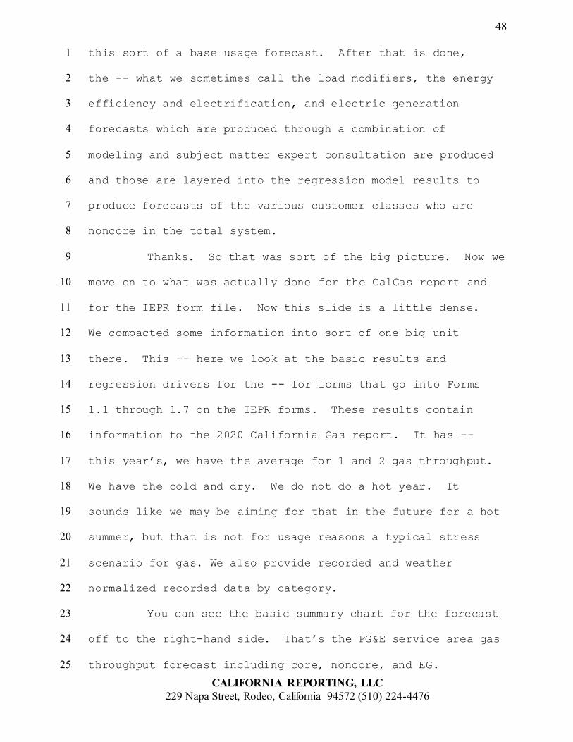
this sort of a base usage forecast. After that is done, 1

the -- what we sometimes call the load modifiers, the energy 2

efficiency and electrification, and electric generation 3

forecasts which are produced through a combination of 4

modeling and subject matter expert consultation are produced 5

and those are layered into the regression model results to 6

produce forecasts of the various customer classes who are 7

noncore in the total system. 8

Thanks. So that was sort of the big picture. Now we 9

move on to what was actually done for the CalGas report and 10

for the IEPR form file. Now this slide is a little dense. 11

We compacted some information into sort of one big unit 12

there. This -- here we look at the basic results and 13

regression drivers for the -- for forms that go into Forms 14

1.1 through 1.7 on the IEPR forms. These results contain 15

information to the 2020 California Gas report. It has -- 16

this year’s, we have the average for 1 and 2 gas throughput. 17

We have the cold and dry. We do not do a hot year. It 18

sounds like we may be aiming for that in the future for a hot 19

summer, but that is not for usage reasons a typical stress 20

scenario for gas. We also provide recorded and weather 21

normalized recorded data by category. 22

You can see the basic summary chart for the forecast 23

off to the right-hand side. That’s the PG&E service area gas 24

throughput forecast including core, noncore, and EG. 25

49



Now the drivers for this forecast are the components 1

from diagram we were looking at on the last slide. We 2

include the recorded sales from PG&E internal data. We 3

include temperature history from PG&E weather database. We 4

include internal rates forecast and economic assumptions from 5

the appropriately vintage Moody’s update which we are a 6

subscriber to. Those are the inputs to what the regression 7

models that we talked about before. 8

Apart from this, we have the load modifiers. Those 9

are the electric generation and the building electrification 10

and energy efficiency and those are going to be described in 11

a little more detail in following slides. 12

So to return to those regression inputs, a lot of 13

them are weather and economic drivers apart from just our 14

internal usage data. 15

Oh, can we back up a slide? Yeah. 16

So that includes our historical age heating degree 17

day data and so our forecast includes that expected heating 18

degree day and a simple climate trend added on top of that. 19

The cold scenario is just a percentile calculated assuming a 20

bell curve distribution for the monthly heating degree days. 21

So that’s our 1 in 10 that we talked about a moment ago. 22

As we said, there’s no cooling degree days because 23

we’re doing a heat stress scenario. One thing that people 24

have asked about that we have not historically done and may 25

50



be valuable, but we have not done this in the past so it’s a 1

significant data exercise, is to break out HDD data by 2

location and map the load forecast to that. 3

For economics, we subscribe to Moody’s service. The 4

residential forecast is driven by population count and 5

households. And the commercial forecast is driven by gross 6

state product localized to the PG&E service area and 7

employment type so that means you checked or service industry 8

or manufacturing, how it breaks out that way because that 9

will drive different components of the throughput. 10

All right, thanks. Next slide. 11

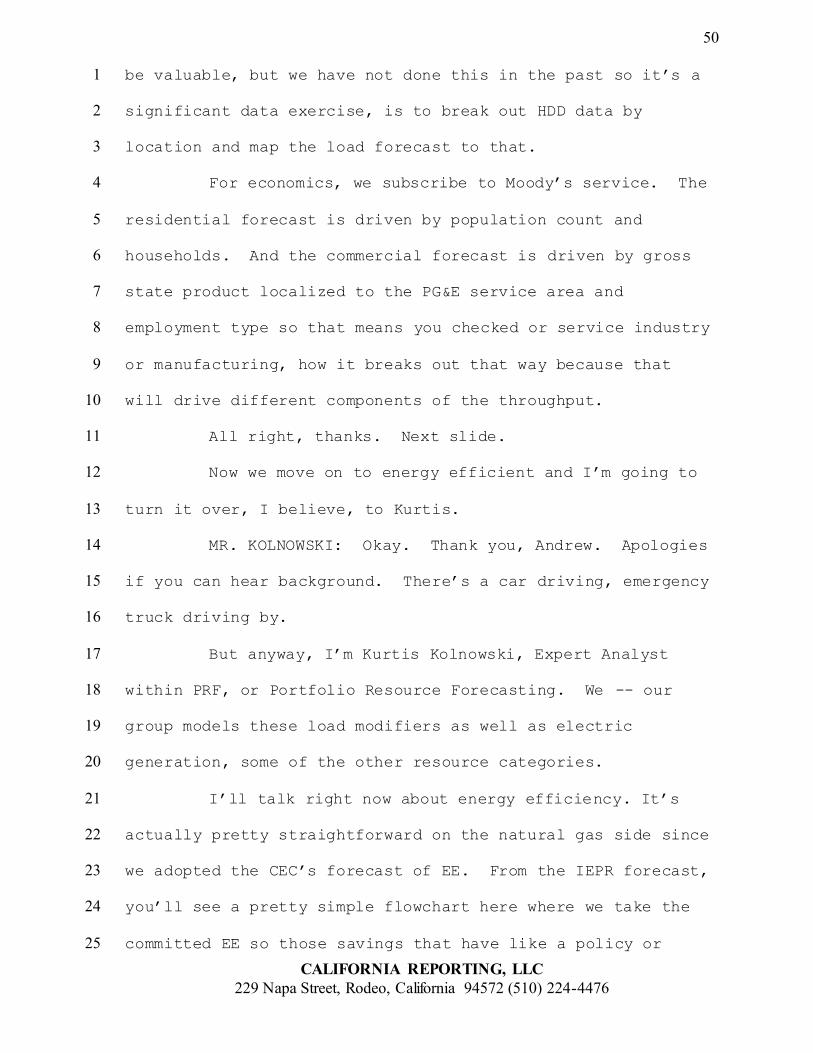
Now we move on to energy efficient and I’m going to 12

turn it over, I believe, to Kurtis. 13

MR. KOLNOWSKI: Okay. Thank you, Andrew. Apologies 14

if you can hear background. There’s a car driving, emergency 15

truck driving by. 16

But anyway, I’m Kurtis Kolnowski, Expert Analyst 17

within PRF, or Portfolio Resource Forecasting. We -- our 18

group models these load modifiers as well as electric 19

generation, some of the other resource categories. 20

I’ll talk right now about energy efficiency. It’s 21

actually pretty straightforward on the natural gas side since 22

we adopted the CEC’s forecast of EE. From the IEPR forecast, 23

you’ll see a pretty simple flowchart here where we take the 24

committed EE so those savings that have like a policy or 25

51



program or code of standard, actually, enacted on the books. 1

And looking at all the different customer clients, 2

residential, commercial as well as AAEE or Additional 3

Achievable Energy Efficiency which comes from several of 4

CPUC’s potential and goals models. And those are where we 5

get future E programs and codes of standards for I believe 6

the CEC also uses or merges a couple of other sources such as 7

beyond codes of standards study which looks a little bit 8

further down the line. But essentially we’re looking to take 9

that data for the PG&E service area and adapt it to our 10

models and use it going forward. 11

So not a whole lot on this one. I will turn over to 12

Amy to talk a little bit about building electrification. 13

MS. KOUCH: Awesome. Can we move to the next slide? 14

All right. Hi everyone, my name is Amy Kouch, and 15

I’m the forecaster who leads the building electrification 16

forecast at PG&E. 17

And so we’ve fill Form 1.10 of the gas IEPR with the 18

building electrification forecast results. And so I’ll be 19

walking you through the high-level methodology of this 20

forecast. 21

So for our forecast, we consider both the residential 22

and commercial sectors and within those sectors we have two 23

building types. We have new construction which are new homes 24

or buildings that are constructed to be all electric. And 25

52



then we have retrofits which are existing gas appliances that 1

are switched to electric at the end of their device lifetime. 2

We then create policy scenarios regarding electrification and 3

then subject matter experts within PG&E will weight the 4

likelihood of these scenarios to occur in order to get a 5

final point forecast. And then our ultimate outputs are the 6

electrical impact, the gas load impact, and peak. These 7

outputs all come from the same model so within the same 8

policy assumptions in order to come up with these different 9

results. 10

And so you might be wondering what our scenarios are 11

actually formed by. You can see that for new construction, 12

it’s really driven by policy. These are our Title 24 13

building codes and Title 20 appliance standards which are 14

updated on a three-year code cycle basis. They also consider 15

reach codes that are passed by local entities. For example, 16

if a city passes a natural gas ban. We work closely with our 17

internal codes and standards team in order to keep updated 18

not just on what current policy is occurring but where we 19

expect future policy to go or could happen until we end up 20

with a summary, like metric of what percent of buildings are 21

considered to be all electric. 22

For retrofits, on the other hand, it’s driven by 23

economics as well as policy and so we create scenarios based 24

on consumer adoption of electrified appliances. So we 25

53



primarily look at space heaters and water heaters, but we 1

also consider cooking stoves, process equipment, and dryers 2

as well. And so the metric we get is percent of existing gas 3

yield appliances that are electrified. 4

And I’m happy to answer any questions in the Q&A. 5

I’ll now pass it back to Kurtis to discuss electric 6

generation. 7

MR. KOLNOWSKI: All right. So the final couple of 8

slides we have are on electric generation forecasting. So 9

this gas, fire, electric generation, climate cycles, gas 10

turbines, reciprocating engines, the various co-gens. The 11

power plants would take the gas off our backbone or local 12

transmission system, convert that to energy, and either use 13

that to serve load on site or sell into an energy market such 14

as the CAISO. 15

So what you’re seeing here is results from the 16

California gas report for PG&E service area. Results are in 17

million cubic feet per day and that’s -- that would be an 18

average over the 365 to 66 days in a year. There’s a couple 19

of things here. The first is since this is a CGR, 2020 was a 20

forecasted year, that’s when the forecast was still being 21

developed. And you’ll see lower Southern California gas 22

prices decrease. EG firms in North Cal, really in that 2021 23

period onward decreasing renewable portfolio standard 24

requirements while reduce EG throughput as well. Since those 25

54



are typically cheaper, they end up generating intermittent 1

resources generate first and EG follows more on the margin. 2

And then finally, in this 2030 to ‘35 period, you see 3

a slight uptick and that’s driven mainly by building 4

electrification or additional electric load on this system. 5

There’s -- once you’re getting out that far, there’s a little 6

bit more uncertainty in what’s actually going to happen. 7

Different resource acquisition exists where de-8

electrification, actually, things like that could result in a 9

pretty wide range in that timeframe, anywhere from really 10

know that increase if there’s electrification load is survive 11

renewables to something like you’re seeing here. And PG&E 12

forecasts, both in average and in CCR 1-in-10 Cold Year, and 13

you’ll see that we both backbone and local transmission plans 14

on here. 15

So going to Slide 9. 16

Okay. So a little bit about the methodology that we 17

used to forecast electric generation. We’re using production 18

cost models. For the CGR, we used MarketBuilder which is a 19

legacy gas generation model. And recently we’ve been working 20

on adapting actually the CEC’s IEPER PLEXOS model for use in 21

EG forecasting. So similar concept, more details. And 22

essentially, we model all the power plants within the WECC 23

loads for those various regions, interconnections, and go 24

step hour by hour and optimize the least cost solution for 25

55



what resources to use to generate to meet the load. 1

I noted a couple of major assumptions that we use for 2

electric generation forecasting on this slide. One of the 3

big ones is electric load. So CEC’s IPER report is used plus 4

we add our own building electrification forecasts within a 5

short-term timeframe. Electrification isn’t the biggest 6

driver but you saw the ’30, ’35 that starts to increase a 7

little bit more. Gas prices are a big driver. For this one, 8

we use prices develop within the CGR. Renewable portfolio 9

standards it’s 50 percent by 2030, consistent with SB100. 10

Also a lot of additional battery storage, a little bit of 11

pumped hydro. Hydroelectric assumptions so how plants within 12

California and then across the WECC. 13

For generate using hydroelectricity, it’s a 14

combination of run of river type systems, mostly out of state 15

that generate as the water’s available. And then in 16

California we have a little bit more control over that. So 17

you can optimize the water levels a little bit more. Once 18

their cooling plant retirements, so the repowers, the 19

retirements coming up, Diablo Canyon in ’25. CO2 prices from 20

the forecast. And then finally on transmission capacity from 21

WECC-wide data. 22

But there’s a lot of assumptions. We work in the CGR 23

and elsewhere with other entities and marketing groups to 24

develop consistency around these. 25

56



And if we can go into Slide 10, I just want to talk a 1

little bit more about assumptions. 2

So this is a little more forward looking here. Up to 3

now, we’ve been talking about how we forecasted to date. I 4

just wanted to call attention to a couple electric generation 5

forecast assumptions that we’ve identified as pretty critical 6

for the future. There’s interest in these, there are 7

substantial drivers, and the environment might be changing 8

(audio lost) in the future. 9

So we talked about this meeting on July 29th, I 10

talked about gas system interdependencies here and we’re 11

currently engaging in statewide studies and working groups 12

such as the IRP, IEPR forecast here. California Gas Report 13

helped address these at a statewide level, but I just wanted 14

to take a quick second to talk about a couple of these that 15

we’re looking at. 16

Hydroelectric generation, as you know, we’re in a 17

drought right now. Over the past 20 years, we’ve observed 18

that there is a trend in declining hydroelectric generation. 19

I want to note, this resource class is highly variable. If 20

you were to draw a line as to what an average looks like, 21

many years would be above or below that line. In fact, in a 22

need for thermal generation so looking into that, assessing a 23

wide range of conditions and seeing what could happen in the 24

future is pretty important given where we are right now. 25

57



Demand forecast is the next one. And there’s 1

impacts, two impacts to call out here, electrification and 2

climate change, potentially. And these can impact both the 3

magnitude of the load needed to be served which would require 4

additional resources and also in climate changes is the 5

variability on this system. So a couple hot days or week, 6

cold winter, those can have a pretty big impact on how 7

electric load is required for -- or electric generation’s 8

required on a specific periods of time. 9

Imports next. So looking at what WECC-wide 10

independencies here. I guess I could call it high -- periods 11

of high overall demand within the WECC, such as some of the 12

heatwaves that we saw earlier this year can constrain imports 13

or resources of the state willing to be -- or available to be 14

imported into California. So really looking at that. I know 15

that’s part of some of the recent preferred system plan work. 16

The CPUC has looked at what our import constraint should be 17

in a peak condition. 18

The next one, future resource additions or 19

retirements. So these impact the resource mix as far as the 20

state’s goals. Just wanted to note that. In this case, 21

there’s a lot of ongoing work on this one. New orders and 22

procurement orders, system plans, things like that. Keeping 23

up to date on those, making sure as those come out, we model 24

those changes, understand where the future’s going, and as we 25

58



transition towards the decarbonization path. We really need 1

to just make sure we stay on top of those as they come out. 2

Finally, this last one, fuel prices. This one 3

doesn’t necessarily affect generation at like CAISO or 4

statewide, but differences between Citygate prices you saw in 5

previous slide decks from the CEC that differences, there’s 6

differences in PG&E and SoCalGas Citygate prices. These can 7

reflect -- these can cause favorable conditions for 8

generators and one region of the state over the other. And 9

understand those price (indiscernible) can help recognize 10

variation of gas to put on utility gas systems. 11

So a lot of these things that we’re looking at 12

working -- want to just, yeah, just draw attention that as 13

things that could have an impact in the future. 14

And that’s actually the end of our slides. So thank 15

you everyone. 16

MS. RAITT: Great. Thank you so much to A.J. Andrew, 17

Todd, Kurtis, and Amy. Appreciate that. 18

So next we will turn to Southern California Gas 19

Company’s presentation on their gas demand forecast. And the 20

two presenters, Sharim Chaudhury who’s the Manager for Cost 21

Allocation and Rate Design and also Jeff Huang, who is the 22

Senior Resource Planner. 23

So go ahead, Sharim. 24

MR. CHAUDHURY: Hi. My name is Sharim Chaudhury. I 25

59



manage the rate design and demand forecasting group for 1

SoCalGas and San Diego on the gas side. And along with me, 2

we have Jeff Huang who’s going to talk about the gas demand 3

for gas fired electrification. 4


So we’re going to talk about a long-term demand for 6

custom models and basically major assumptions underlying sort 7

of each of those models. So we have models for our core 8

market segments and we have separate models for noncore 9

customers including electric generation customers. And we’ll 10

talk a little bit about the weather design because it’s an 11

important element of long-term demand forecast for our 12

customer segment whose gas demand is weather sensitive. 13

Then we’re going to talk about cold year demand. As 14

PG&E talked about in the California Gas report, we provide 15

two scenarios. One is sort of average year demand and other 16

is cold air, dry hyrdo demand. These two scenarios. In 17

addition, we also will briefly talk about the peak day demand 18

for our system. And then at the end, we’ll share a few 19

slides about our forecasting results from the 2020 California 20

Gas Report. 21

Next slide. 22

This is an exhaustive list of the long-term demand 23

forecasting model we have by core and noncore customers and 24

also by wholesale customers. So as you can see in this 25

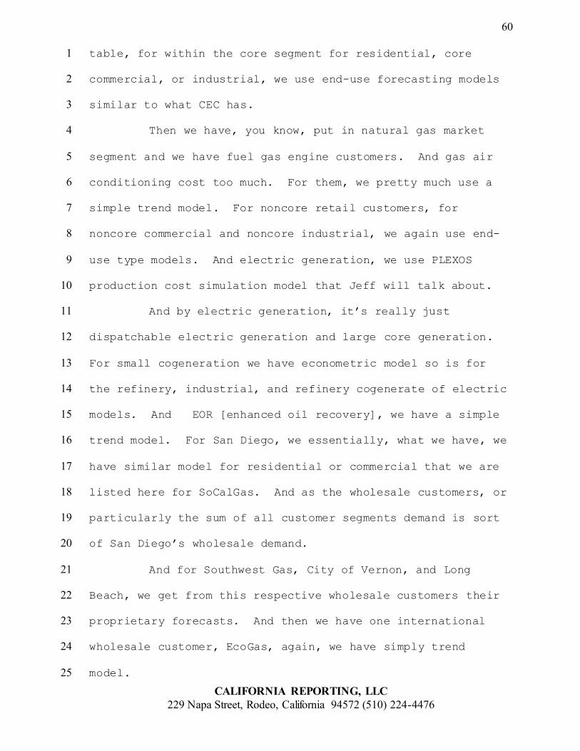
60



table, for within the core segment for residential, core 1

commercial, or industrial, we use end-use forecasting models 2

similar to what CEC has. 3

Then we have, you know, put in natural gas market 4

segment and we have fuel gas engine customers. And gas air 5

conditioning cost too much. For them, we pretty much use a 6

simple trend model. For noncore retail customers, for 7

noncore commercial and noncore industrial, we again use end-8

use type models. And electric generation, we use PLEXOS 9

production cost simulation model that Jeff will talk about. 10

And by electric generation, it’s really just 11

dispatchable electric generation and large core generation. 12

For small cogeneration we have econometric model so is for 13

the refinery, industrial, and refinery cogenerate of electric 14

models. And EOR [enhanced oil recovery], we have a simple 15

trend model. For San Diego, we essentially, what we have, we 16

have similar model for residential or commercial that we are 17

listed here for SoCalGas. And as the wholesale customers, or 18

particularly the sum of all customer segments demand is sort 19

of San Diego’s wholesale demand. 20

And for Southwest Gas, City of Vernon, and Long 21

Beach, we get from this respective wholesale customers their 22

proprietary forecasts. And then we have one international 23

wholesale customer, EcoGas, again, we have simply trend 24

model. 25

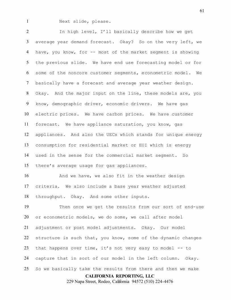
61




In high level, I’ll basically describe how we get 2

average year demand forecast. Okay? So on the very left, we 3

have, you know, for -- most of the market segment is showing 4

the previous slide. We have end use forecasting model or for 5

some of the noncore customer segments, econometric model. We 6

basically have a forecast and average year weather design. 7

Okay. And the major input on the line, these models are, you 8

know, demographic driver, economic drivers. We have gas 9

electric prices. We have carbon prices. We have customer 10

forecast. We have appliance saturation, you know, gas 11

appliances. And also the UECs which stands for unique energy 12

consumption for residential market or EUI which is energy 13

used in the sense for the commercial market segment. So 14

there’s average usage for gas appliances. 15

And we have, we also fit in the weather design 16

criteria. We also include a base year weather adjusted 17

throughput. Okay. And some other inputs. 18

Then once we get the results from our sort of end-use 19

or econometric models, we do some, we call after model 20

adjustment or post model adjustments. Okay. Our model 21

structure is such that, you know, some of the dynamic changes 22

that happens over time, it’s not very easy to model -- to 23

capture that in sort of our model in the left column. Okay. 24

So we basically take the results from there and then we make 25

62



some adjustment for that. So like PG&E described that for EE 1

savings, you know, we do after model adjustments. And the 2

EE, energy efficiency elements that we capture is exactly 3

like PG&E described. It’s committed and also additional 4

achievable energy efficiency. You know, the goal that the 5

Commission decides on. 6

Then we also model climate change. Global warming, 7

in fact, that’s also up to the model or post model 8

adjustment. Then we have some customer migration from 9

noncore or vice versa, we do that. 10

So then we come up in the final forecast which is 11

essentially repeating the sort of average year weather design 12

so what we get is the average year demand. And on a very 13

high level, you know, for the forecast of residential 14

customers in demand growth is the new housing starts is the 15

main driver for the residential market segment. And for the 16

commercial industrial market forecast is really the projected 17

employment groups over time. 18


This -- end-use models are extremely data-intensive 20

model. And it’s partly sort of for like a inventory tracking 21

model. It basically figures out for customers what household 22

or commercial industrial customers energy used essentially is 23

through the different gas appliances they have and the use of 24

it. And two quick key steps particularly at a point in time 25

63



would be in appliance stock they have and also it charts in 1

the collection of this appliance stock whether it’s space 2

heating, water heating, clothes dryer, or cooking, for 3

example, and whether they choose a gas or electric appliance. 4

And also once they choose it, they’re in charge of the 5

efficiency level and they can purchase, you know, high 6

efficiency or standard efficiency. 7

As the simulation steps forward from one year to 8

next, we keep track of -- the models keep track of each year 9

between new load added due to new meters or new customers. 10

In addition to for existing customers, you, for example, some 11

of their appliances become worn out and then they make a 12

decision of new appliances for their new place, gas 13

appliances, gas appliance or electric appliance and the 14

associated energy efficiency for those appliances. 15

Now base year forecast is calibrated to base year 16

historical weather normalized consumption. Now as you know 17

for the long-term demand forecast, you know, weather is very 18

hard to predict so the long-term demand forecast we basically 19

forecast gas demand under normal weather condition. And the 20

way we define normal is sort of an average of historical 20-21

year average. 22

And so one of the salient feature of the annual 23

forecasting model is the calibration approach. So for the 24

2020 CGR, 2019 we call it the base year. So when we 25

64



developed a forecast, 2020 forecast, we had historical data 1

from 2019 and we also used the end use forecast model to 2

develop up the forecast of 2019. And the calibration really 3

means that we come up with the forecast for 2019, the base 4

year, and compare that with the actual consumption. 5

Actually, not actual consumption, take actual consumption and 6

weather normalize it. Okay. And to the extent that weather 7

normalized, historical consumption was higher and lower than 8

the forecast. We basically calibrate or adjust the forecast 9

up and down so it matches. 10

Okay. Next slide, please. 11

So for the noncore customers, as I mentioned, every 12

year we have econometric model, models for SoCalGas refinery 13

industrial and refinery cogent customers. The sort of 14

exploratory variables of the econometric model of the gas and 15

the propane prices. You can think of to get propane prices 16

are competing input in the gas prices lower, the refinery’s 17

going to use gas and vice versa. The propane prices lower 18

than they are going to use propane instead of gas. 19

For SoCalGas small cogeneration is again, well, it’s 20

driven by the gas price and the electricity price. You can 21

think of it as the input price and the output price. So if 22

the electricity price is very high compared to the cost of 23

producing electricity, then they’re going to use the gas. 24

For enhanced oil recovery, we use a simple historical 25

65



trend. It could be average of last three years or five 1

years. 2


So here we’re talking with the post model 4

adjustments. We talked a little a bit about the energy 5

efficient savings and that’s really PG&E described in great 6

detail what those savings are so I’ll just quickly go and 7

move to the next one. 8

Weather designed to account for -- sorry, sorry, if 9

you could go back to the previous slide. Yeah. 10

So I want to point out weather designed to account 11

for global warming. In the 2020 CGR, for the first time, 12

we’ve basically incorporating the fact that on average, 13

winters are getting warmer so we have fewer and fewer HDD on 14

average. Okay. So for the forecast period, we projected an 15

annual HDD reduction of about four heating degree days each 16

year for SoCalGas. 17


So we essentially talked about a previously, you 19

know, our average year demand forecast. And then the second 20

scenario or for the weather sensitive load, we have come up 21

with a 1-in-35-year cold year demand forecast. And if you -- 22

you can see the process as in a cold year demand, gas demand 23

will be higher than the average year gas demand. And the 24

incremental gas demand really depends on average year, 25

66



weather design, and 1-in-35 cold year weather design and 1

basically what the -- the average demand was associated with 2

the average year is to HDD design and basically we have 3

historical relationship between sensitive and between how 4

much gas demand changes if heating degree days change by one 5

and then for each market segment. 6

Okay. So this incremental cold year demand is 7

derived by this element that we -- the bullet points we have 8

highlighted in one, two, three, and four. And the average of 9

demand average year is to be designed 1-in-35 cold years to 10

be designed and demand sensitivity per HDD. 11

Now the, for us, the weather sensitive market 12

segments are residential or commercial or industrial. 13

SoCalGas’s noncore commercial, these are the customers 14

segments which we consider HDD sensitive market segments. 15

For non-HDD sensitive market segments, cold year demands are 16

basically the same as the average year demand. 17


So we also calculate peak day demand and we have 19

basically two scenarios. One is 1-in-10 year peak day at 20

temperature design which is 42.2 degrees Fahrenheit. And for 21

1-in-35 peak days in temperature design is 40.5 degrees 22

Fahrenheit. And both of these sort of these degree 23

Fahrenheit are based on we look at annual coldest day HDDs 24

over the last 70 years starting in 1950 and going through 25

67



2019. Okay. 1

And the way I described how we come up with sort of 2

incremental gas demand in 1-in-35 peak year. So the 3

analogy’s similar. What we do is that we look at sort of 4

average cold day demand which would be an average day in 5

December and we basically look at what is the incremental gas 6

demand for peak day in December. And the way we come up with 7

is when the in core peak day temperature design which we 8

talked about in bullet one and two, then we look at average 9

year demand 1-in-35 cold year demand and then we come up with 10

the sensitivity, you know, to peak day -- to daily demands to 11

HDD. 12

Next slide, please. Next slide. 13

So Jeff will talk about the next couple of slides. 14

MR. HUANG: Okay. My name is Jeff Huang. I do the 15

EG gas demand forecast for SoCalGas. And in late 2019, we 16

licensed PLEXOS production cost simulation model from energy 17

exemplar. And because CEC has a very comprehensive database, 18

we basically download the CEC’s spring 2020 database as our 19

reference case. And then we make changes on top of that as 20

needed. 21

And for 2020 CGR, we selected and met demand case 22

with mid-AAEE case. That’s our electricity demand for our 23

simulation. And then we made additional changes such as we 24

inputted the updated compliance schedules per State Water 25

68



Board and we extended the retirement date of Alamitos, 1

Huntington Beach, Ormond Beach, and Redondo Beach. 2

Next slide. 3

And I think this is a major deviation from the CEC’s 4

forecast. For the natural gas price forecast, we did not use 5

the CEC’s forecast. We used the market price reference 6

methodology. It is a combination of the NYMEX Futures and 7

other long-term gas price forecasts. And at the same time, 8

we updated where as needed and we make sure that renewable 9

resources is 60 percent RPS goal by 2030, and we kept it at 10

60 percent for 2035. 11

And so for most of the database, we followed CEC’s 12

database and we want to be in sync with their database so 13

that we are on the same page. And our general methodology is 14

when we get the new database, we do a sanity check, and then 15

we provide feedback back to CEC for any corrections so that 16

as we move forward, all databases will be in sync. 17

And so another -- for CGR 2020, we do two scenarios; 18

average year hydro scenario, and the 1-in-10 dry hydro 19

scenario. I believe the average year hydro scenario is in 20

the CEC database, it’s based on a 15-year average. And then 21

we select a year that meets the 1 in 10 dry hydro conditions. 22

And for the CGR 2020, we selected hydro year 2015. 23

And for the next CGR, for the CGR 2022, we hope to 24

use CEC’s most recent database as of spring 2022. And again 25

69



we will follow the same methodology and provide any feedback 1

back to CEC on the data in our service territory. 2

And now back to Sharim for the results. 3

MR. CHAUDHURY: Next slide, please. Next slide. 4

As we mentioned earlier, for the residential market 5

segment, new housing starts basically a significant driver 6

for the long-term demand forecast. So this chart is from the 7

2020 CGR report. So in southern California, what we are 8

observing is that new building is slowing down but their 9

record low interest rates are expected to bring strong 10

recovery. 11

And if you look at this slide, you know, it says 12

historical sort of housing starts from 1990 on ward and it 13

goes up to the forecast period of 2035. And as you see that 14

in the great recession of 2008 and ’9, the housing started to 15

decline significantly and it has picked up and with this low 16

interest rate, we think it’s going to pick up even more. 17

And one of the observation is since the last 2008, 18

2009 if you will observe the proportion of multi-family 19

housing starts -- is sort of proportionately more since 2010 20

compared to the time period before 2010. Just interesting to 21

note. So we had a low of 20,000 2009 and for 2019, we have 22

seen sort of 51,000, you know, it’s forecasted to be 70,000 23

in 2023 and 61,000 in 2035. 24


70



Here we are looking at sort of our active number of 1

meters and meter growth. So the orange bars basically shows 2

the meter growth and the black line basically shows number of 3

active meters in millions on the right-hand side scale. 4

Whereas that meter growth is on the left-hand side scale. So 5

actual 2019 active meters for us was 5.8 million and we are 6

seeing sort of an average annual growth. We are expecting 7

over the forecast period of 0.6 percent. 8


Major legislations affecting the forecasts in the 10

2020 CGR. For Senate Bill 100 is for that eligible renewable 11

energy and zero carbon resources supply 100 percent of retail 12

sales in electricity in California by 2045. It also calls 13

for renewable energy to supply 50 percent of the state retail 14

electricity by 2026 and 60 percent by 2030. And Jeff has 15

incorporated sort of these assumptions in his EG gas demand 16

forecast. 17

For energy efficiency Senate Bill 350, the goal is 18

double the cumulative energy efficiency savings by 2030. And 19

these state energy efficiency projections we have included in 20

our 2020 CGR forecasts. 21

For Assembly Bill 3232, you know, calls on state 22

agencies by 2021 to develop plans and projections to reduce 23

greenhouse gas emissions in California’s residential and 24

commercial buildings to 40 percent below 1990 level by 2030. 25

71



So we have not included sort of the gas demand reduction 1

associated with greenhouse gas reduction in the 2020 CGR. 2

Going forward we are -- in the 2022 year we are thinking 3

about including some scenarios. PG&E had some scenarios in 4

the 2020 CGR and they talked about it briefly and we’ll have 5

some scenarios most likely in the 2020 CGR. We have not 6

defined these scenarios yet. 7

Next slide. Next slide, please. 8

So this is sort of the summary from the 2020 CGR gas 9

demand forecast sort of overall in the high level by 10

residential, core nonresidential, noncore non-EG, and 11

electric generation, and wholesale customer group. So the 12

total order expected to fall between 2019 and 2035 declining 13

an average of 0.9 percent per year. And for comprehensive 14

purposes, they sort of -- the rate of decline is higher if we 15

compare it with the 2018 CGR and also with the prior 2016 16

CGR. And primarily, the reduction is from energy efficiency 17

program savings offsetting, you know, the meter growth and 18

the employment growth. 19


And here basically we talk about what are the change 21

in demand by customer segments. For residential, gas demand 22

declines about 1 percent between 2020 and 2035. And again 23

declining use for meter more than offsets the meter growth. 24

And since 2021m weather-normalized residential use 25

72



for active meter has been dropping by 0.6 percent per year. 1

Commercial gas demand is expected to fall by an average of 2

1.1 percent per year. Industrial load is expected to decline 3

by 0.6 percent from 2020 to 2035. 4


Wholesale, excluding SDG&E is expected to shrink 6

slightly between these forecast periods. San Diego’s gas 7

demand is forecasted to decrease an average of 0.6 percent 8

per year. NGV load are expected to grow by 1.4 percent per 9

year and it’s largely due to low carbon government incentives 10

and low natural gas prices relative to gasoline and diesel. 11

And carbon offsetting renewable natural gas already fuels 12

about 80 percent of our territory natural gas vehicle load. 13

Enhanced oil recovery steaming demand is forecasted to remain 14

steady, you know, throughout the forecast period. 15


You’re not talking about it, Jeff? In the EG demand 17

forecast? Are you in it? 18

MR. HUANG: The EG demand forecast is expected to 19

decrease over time. And, I mean, it’s largely due to the 20

increase in renewables. And it’s -- the renewable is mostly 21

displacing the natural gas. And then for the dry hyrdro 22

scenario, we notice that the dry hyrdo has lesser impact than 23

prior CGRs and we think that’s largely due to the increase in 24

renewables. We have RPS reaching 60 percent by 2030 so 25

73



there’s a significant amount of renewable generation to 1

displace the hyrdo. 2

Okay. Back to you, Sharim. 3

MR. CHAUDHURY: Next slide, please. 4

I guess we are done. 5

MS. RAITT: Thank you, Sharim. 6

Commissioners, we have a little time for discussion 7

if you have some questions or comments for Jeff and Sharim. 8

COMMISSIONER GUNDA: Yeah. So thank you, Jeff and 9

Sharim and the PG&E team for all the presentations. I think 10

it’s really, really helpful to see how you’re considering 11

various aspects moving forward. 12

I know there’s a bunch of questions that came through 13

Q&A so I’m going to ask one question and then see if 14

Commissioner McAllister has any and then go to Q&A and then 15

we can come back if there is time. 16

So the high level, Sharim, I think specifically you 17

mentioned about climate change impacts being talked through 18

in terms of adjustments to the heating degree days. 19

MR. CHAUDHURY: Uh-huh. 20

COMMISSIONER GUNDA: Just wanted to ask what the PG&E 21

team and you, maybe Andrew might want to comment on this, one 22

is kind of rationale behind decreasing by 4 heating degree 23

days, reducing by 4 heating degree days. And what are PG&E 24

doing similar to capture climate change impacts? 25

74



MR. CHAUDHURY: Okay. So this is Sharim, let me just 1

try to explain what is the rationale for decreasing heating 2

degree days by 4. So our average heating degree days per 3

average year, we basically calculate over a 20-year period. 4

And we have an actual historical data, so we have calculated 5

sort of 20 numbers of 20-year average heating degree days 6

based on going into the future. Okay. 7

So we have this 20 data elements and basically based 8

on that, we basically looked at the trend, okay, how the 9

heating degree days over this 20-year average heating degree 10

days has changed over this 20 of the observation points 11

through regression analysis, and we found out that it’s about 12

4 degrees -- 4 heating degree days. 13

COMMISSIONER GUNDA: Thank you, Sharim. 14

Maybe Andrew or Kurtis has -- wants to share anything 15

from PG&E and I just have a quick follow up. 16

Andrew, you’re muted if you’re speaking. 17

MR. KLINGLER: There we go. Yes, on the regression 18

side, we have looked at the California climate adaptation 19

forecast and so we’ve done a very simple linear interpolation 20

of that going out to about 2040. And so we have a 21

coefficient that increases the number of -- excuse me, 22

decreases the number of HDD over time. And I would have to 23

look up the exact amount, but it’s about .6 per -- .6 HDD per 24

year. 25

75



COMMISSIONER GUNDA: Right. So I think just a follow 1

up to both of you. So one of the thing on the electricity 2

demand side, at least given the level of the concerns we’ve 3

had the last couple of years, it has been this consideration 4

that, you know, history’s not a good indicator of the future 5

in terms of the uncertainty and the volatility that we might 6

see in the fluctuations. 7

Has there been thinking about how to capture future 8

uncertainties and volatility around temperature, drought, and 9

so on? Just your high-level talks on how that would helpful. 10

MR. KLINGLER: I’ll go first, if that’s okay. What 11

we have really started moving toward internally and probably 12

would prefer to do externally also is to move towards a 13

scenario analysis based approach where we instead of trying 14

to estimate something like statistical variation or we would 15

specify actual possible scenarios that might play out. And 16

that would include both climate scenarios and policy 17

scenarios because obviously as we move forward, that’s a big 18

driver. 19

MR. CHAUDHURY: Commissioner, you brought up a good 20

point. So what happened is that for -- due to climate 21

change, the average heating degree day per year is declining. 22

But as you pointed out, the volatility, okay, it could be 23

become more intense. So what we are finding out from some 24

work we have done is that even though the average year 25

76



throughput is going down, peak day demand not naturally is 1

coming down as much. 2

COMMISSIONER GUNDA: Got it. 3

MR. CHAUDHURY: Okay. 4

COMMISSIONER GUNDA: Thank you, Sharim. Thank you so 5

much. 6

I’ll pass it on to Commissioner McAllister and then 7

we’ll go to Q&A. 8

COMMISSIONER MCALLISTER: Thank you, Commissioner 9

Gunda. So you read my mind kind of on that, you know, 10

future, you know, sort of expanding envelope of possibilities 11

going out and how we’re going to capture that is, you know, 12

the past is not a good predictor. So that’s an interesting 13

ongoing discussion. 14

My question just has to do with the 3232 world, both 15

PG&E and SoCal. I was happy to see you mention the 3232 16

report and those scenarios are pretty stark in terms of what 17

we told the legislature would need to take place in order to 18

get the building sector to 40 percent below 1990 level. And 19

there’s, you know, in order to do that the takeaway is pretty 20

much massive fuel substitution from gas end uses to electric, 21

certainly in a residential sector where it’s most prevalent. 22

And I guess I’m wondering a couple of things about 23

that. You know, one did you do true, I think SoCalGas did 24

not, I had to step away a little bit so I didn’t hear fully 25

77



what PG&E is doing on that. But, you know, I guess I would 1

just ask if you have done and encourage you to do, if not, 2

some full sort of 3232 scenarios just to see where that 3

leads. You know, maybe it’s a bookend, maybe it’s not, but I 4

think that would be helpful how have you contemplated those 5

scenarios in each of your respective forecasts? 6

MR. CHAUDHURY: Andrew, do you want to go first? Or 7

I can go. 8

MR. KLINGLER: You can go ahead, if you like. 9

MR. CHAUDHURY: Okay. 10

MR. KLINGLER: I have a few people on the team. 11

Yeah. 12

MR. CHAUDHURY: Yeah. Commissioner McAllister, we 13

are looking into the scenarios. Okay. I mean, the way we 14

particularly, we do it is that as we discussed, you know, in 15

the California Gas Report, we pretty much had in terms of 16

truthful forecast we put for, you know, two scenarios. One 17

is the average year and one is a cold year dry hydro. And it 18

seems like when this decarbonization goes, we probably need 19

to have additional scenarios including maybe some bookends 20

like you mentioned. Okay. 21

The reason is that, you know, our demand forecast, 22

like 1-in-10 year, 1-in-10 cold year demand forecast and the 23

peak day demand forecast that used for our transmission 24

planning purposes, right. So we have started talking 25

78



internally, we’re not in a position to basically say much. 1

But I feel like we probably need to have additional scenarios 2

in the California Gas Report. 3

And why I said that is that sometimes we are ask to 4

pick a point estimate, what do you think is the best 5

forecast, right. And that point estimate gets very 6

difficult, you know, in the future, right, when this 7

decarbonization scenario what is likely versus goal. Because 8

as you know for our cost allocation and rate design, we use 9

sort of, we come up with the rate is revenue to curve and 10

divided by average year throughput. And average year too 11

could be significantly different depending on the level of 12

decarbonization. 13

And likewise, you know, we are supposed to have a 14

reliable transmission system, okay. And for slack capacity 15

on our transmission system, we look at 1-in-10 cold year 16

average day throughput. And this issue has come up in the 17

gas OIR sort of track one issue. 18

So, I mean, we probably need to put forth more 19

scenarios but the end of the day we need to figure out if 20

somebody asks us to give a point estimate, what do we point 21

to. 22

COMMISSIONER MCALLISTER: Thank you for that. I 23

would agree, some additional scenario work and also the 24

crosswalk over with the electric side, right, just because 25

79



SB100. Not every, you know, sort of unit of energy 1

consumption that migrates from a gas end use to an electric 2

end use is going to actually imply the same amount of carbon 3

on the electric side, right, depending on the scenario. 4

So I think there’s a pretty nuance sort of co-5

scenario development maybe that ought to take place here to 6

capture fuel substitution. And, I’m sorry, I got in front of 7

you, Andrew, so go ahead. 8

MR. KLINGLER: No, that’s fine. I’m -- yeah, we 9

similarly we have, we’re in a world where we’re working with 10

point forecasts and not have done a lot of super 11

sophisticated work beyond that. We do have the 12

electrification forecast that you see here and that we update 13

regularly. That is actually set up in a way that’s 14

consistent between the gas and electric side. So there is an 15

estimation exactly of how that energy is being traded off. 16

The accuracy of that kind of thing, of course, 17

depends heavily on, I mean, it’s not going to be super 18

precise and it also depends itself on assumptions about 19

policies that are behind the way things play out. 20

COMMISSIONER MCALLISTER: Okay, yeah, great. Thanks 21

very much. I appreciate those answers. 22

We have some really good questions in the Q&A so I 23

want to ask to pass to the moderator for Q&A. So I think 24

that’s Jennifer Campagna? 25

80



MS. CAMPAGNA: Yes, it is. Thank you, Commissioner. 1

Okay, so to start off, Tom Beach has a two-part 2

question and this is for PG&E. 3

Is the PG&E electric generation throughput forecast 4

consistent with the adopted CPUC 2030 GHG emissions of 46 MMP 5

in the IEPR reference system portfolio? 6

Part two, if the 2030 GHG goal is reduced to 38 MMP, 7

how much would the EG forecast decrease? 8

And I’ll turn it over to anyone in PG&E who would 9

like to answer. 10

MS. RAITT: Andrew, I think you’re muted. 11

MR. KOLNOWSKI: I think Todd Peterson has a response 12

to these. That’s probably double muted. I can respond to 13

this myself. 14

So two-part question. The first is what assumption 15

was used in the CGR? And the second, how would EG change 16

using that more stringent GHG reduction target? 17

So the first one, CGR does use the preferred -- or 18

the reference system plan 46 million tons. I believe that 19

was a compilation of February of 2020 that’s cited in the 20

CGR. 21

The second one, that GHG target -- or using the more 22

stringent GHG goal, that’s a place where we’re definitely 23

looking to conduct additional analysis particularly around 24

updated portfolios that may target that. I know that the 25

81



CPUC is proposing a preferred system plan looking at 38 MMT. 1

So I would expect this to be a source of frequent discussion 2

in the upcoming months. 3

MS. CAMPAGNA: Thank you. Is there anyone else from 4

PG&E? Okay, great. 5

The next question is for both PG&E and SoCalGas and 6

it is from Mike Florio. If overall residential and 7

commercial average gas demand are trending downward, is there 8

any reason to expect peak demand for these customers to 9

follow a different trend? 10

And we can start with if PG&E would like to do the 11

first response followed by SoCalGas. 12

MR. PETERSON: Hi, this is Todd Peterson with PG&E. 13

The way to think about what’s happening on the demand 14

side as observed demand over long-term declining, I think a 15

good way to take a look at this is that the forecast that we 16

have in the 2020 CalGas Report. There was one perspective of 17

looking at the abnormal peak day demand which are -- is an 18

extreme condition forecast. And that is that they 1-in-90 19

cold temperature event to ensure that our PG&E system can 20

meet that peak demand for core customers. 21

So that’s in the CalGas Report, you can see that. 22

There is over the three-year period that we are forecasting 23

for abnormal peak day, or APD, there is a slight uptick in 24

core demand. 25

82



Secondly, there is also a summer and winter peak day 1

forecast. And in general, those demands are flat to 2

declining in both those periods of winter and summer. 3

I think that’s a good area to start with and I think 4

that there’s an area to do more study in how demand would be 5

changing as the system changes with more renewables on 6

system. We see electrification growing. There is still a 7

lot of uncertainty around this, an unknowing. So the 8

scenario analysis should help us understand that better. 9

MR. CHAUDHURY: Okay. Think about -- I think if the 10

ever reached for residential market segment toward the 11

average usage to go down, peak demand might not change much, 12

you know. Think about for residential market segment, gas 13

big demand happens either in December or January. 14

Think of what -- we can think of a situation that 15

they could be cloudy or rainy where we may not have, you 16

know, solar providing sort of the electricity so we may have 17

to meet the residential sort of heating demand. We may have 18

to fire up the gas, you know, stand by peaker unit, for 19

example. So it’s not a one-to-one reduction, you know, for 20

if the average demand goes down, peak demand might not 21

necessarily go down. 22

MS. CAMPAGNA: Okay. Thank you. Appreciate it. 23

Okay, so the -- looks like the last open question we 24

have is from Katie Elder. And the question is for Sharim. 25

83



Sharim, are you seeing the 42.5 degree increase as 1

your 70 years rolls forward? 2

MR. CHAUDHURY: You know, for peak days, you know, 3

weather design, we basically have not rolled in 70 years, we 4

just, you know, the oldest data we captured in 1950 and 5

basically additional cold days the year progress, we 6

basically add to it. 7

Now what happens that we are picking up the coldest 8

day for each of those 70 years. And if we add one or two 9

more years, it’s really is not impacted the tail end of the 10

distribution as much, as I recall from last year. So I think 11

it’s not changing much. That would be my answer now but I 12

can look into that. 13

MS. CAMPAGNA: Okay. Thank you, Sharim. 14

So we actually have another -- one more question, a 15

follow-up question from Mike Florio. I understand that 16

average and peak may decline at different rates, but is there 17

any logical reason why peak would increase when the average 18

is declining? 19

MR. CHAUDHURY: Yeah. For SoCalGas, we have not 20

looked at the essential peak demand in particular. Maybe we 21

should look at that. We basically look at sort of system 22

peak. I couldn’t answer the question now, okay, but the idea 23

is that if -- because of, if in the future, for example, 24

someone is heating demand is transferred to, based on say 25

84



electric heat pump and things like that. And if we do have, 1

for example, a cloudy day, I don’t know if the peak demand 2

could go up or not. But it’s, my first guess is Mike is 3

unlikely. 4

MS. CAMPAGNA: Okay. Thank you. Is there any follow 5

up from Todd or anyone at PG&E on this question? 6

MR. PETERSON: Hi, it’s Todd Peterson from PG&E. We 7

don’t have the right experts here to really uncover this a 8

little bit more. It’s something that we would need to get 9

back to you. 10

MS. CAMPAGNA: Okay. Thank you, everyone. 11

That is it on our open Q&A on our Zoom session. 12

Heather, I will turn it back to you. Thank you. 13

MS. RAITT: Great, thank you. And so, thank you, 14

Jennifer, for leading us through that. 15

Commissioners, if you didn’t any have -- or if you 16

have any final comments or questions for the utilities; 17

otherwise, we will move on to public comment. 18

COMMISSIONER MCALLISTER: Thank you. Thank you very 19

much. 20

MR. RAITT: Commissioner Gunda, we can’t hear you. 21

COMMISSIONER GUNDA: Thank you, double mute. 22

Thank you so much again, Andrew, Amy, Todd, and 23

Kurtis, Sharim, and Jeff for being here. I mean, I know the 24

forecasting in the modeling part is such a grueling task. So 25

85



it’s definitely something that is self-selected by people who 1

like to do those things. So I really appreciate all the work 2

and time to be here. 3

And I think my way of comment is, you know, as we 4

move forward, I think what Andrew noted this and Sharim, the 5

importance of looking through scenarios and then having 6

adequate participation of possible futures to guide policy. 7

It is important. 8

I think it kind of goes through both, you know, 9

electrification and the end use policy scenarios, the weather 10

scenarios. But also looking at it from a temporal and 11

geographical distribution as well. So I look to your 12

continued efforts in improving the forecast and working at 13

CEC to improve analytics as well. Perhaps as a state, we can 14

have a good set of forecast data to make decisions. So thank 15

you all so much for being here and helping us through this 16

conversation. 17

MS. RAITT: Super. All right, Commissioner, we’ll go 18

on to public comment and thank you again. 19

Right now we have RoseMary Avalos to lead us to 20

public comment. Go ahead, RoseMary. 21

MS. AVALOS: Thank you, Heather. 22

Commenters, please allow one person per organization 23

make a comment and comments are limited to three persons -- 24

three minutes per speaker. 25

86



And I’ll move on to those on Zoom. I see that Frank 1

Seres has his hand raised. 2

Frank, your line is open. You may need to open on 3

your end. Frank, you may need to open on your end. 4

Okay. I’ll move on to Mike Florio. Please state 5

your first and last name and spell that, as well as if you 6

have an affiliation, please state your affiliation. 7

Go ahead and speak. You may need to unmute on your 8

end. Go ahead and speak, Mike. 9

MR. FLORIO: Okay, I’m trying to. 10

MS. AVALOS: We can hear you. We can hear you. 11

MR. FLORIO: Okay. Yes, Mike Florio, F-L-O-R-I-O. 12

I’m an independent consultant. And I just wanted to raise a 13

question about the rate escalation assumption for 14

transportation rates for gas. A 2.3 percent seems 15

remarkably low to me. PG&E’s current rate base is looking at 16

a 18 percent increase in the gas revenue requirement with 17

further attrition issue that increases every year to follow. 18

So that’s not rounding error from 2.3 percent. 19

That’s quite substantial and I think SoCalGas’s last rate 20

increase is well more than that small percentage as well. So 21

I think you would want to take a close look at those 22

assumptions because it certainly seems like that rate of 23

increase, if anything, is accelerating. 24

That’s all I have. 25

87



MS. AVALOS: Okay. Thank you, Mike. 1

And I think Frank Seres, your mic is open. 2

Okay. Seeing that there are no hands raised on Zoom, 3

now I’ll move on to the phone lines. And a reminder for 4

those on the phone to dial star 9 to raise your hand and star 5

6 to unmute. Okay. So let’s give a second for those on the 6

phone to if you want to raise your hand. 7

Okay. Seeing that there are no raised hands, that 8

completes public comment. 9

I turn now to Commissioner McAllister. 10

COMMISSIONER MCALLISTER: Thank you, RoseMary. 11

So, Heather, correct me if I’m wrong, that’s it for 12

the day if we have no more questions from the dais or and 13

there are no more panels. So. 14

MS. RAITT: That’s right, you’re done. 15

COMMISSIONER MCALLISTER: Great. Okay. I guess I 16

would just say thank you to Commissioner Gunda for your 17

stewardship of this and your leadership and just, you know, 18

your deep knowledge of this really helps the conversation 19

keep grounded and bring in new information in a really, 20

really good way. So I really appreciate all your guidance on 21

this. 22

And I would just say, you know, okay, with the caveat 23

that, yes, it’s a bunch of gas nerds in the room here. This 24

is big stuff, actually. The way we’re really modernizing the 25

88



gas side of the house to match up with the electric side and 1

in all the ways that Commissioner Gunda mentioned. And so I 2

think that increased regularity and temporal appreciation, 3

and the interlinkages, you know, that we put in place across 4

the electric and gas forecast increasingly, and work with the 5

utilities to do that as well on their side. And then really 6

match those up and work through all these issues in an open 7

way is real critical. 8

It’s just, it’s -- that process can really make some 9

better product and it’s essential to getting it right and 10

rolling with reality over time, so I’m really appreciative of 11

this process and the presentations here today both from staff 12

and from utilities. 13

With that, I think we’re in a good place and building 14

those communication bridges to really be continually drilling 15

on the issues as they come up and then move forward to 16

constructive forecasts itself. 17

So I pop back to you, Commissioner Gunda. 18

COMMISSIONER GUNDA: Yeah, thank you, Commissioner 19

McAllister. I couldn’t say that better. I know I just want 20

to thank the staff. You know, we’ve been going so many 21

different directions over the last especially 18 months. 22

Some heavy lifts from SB 100, AB3232, the building code and 23

all of that has direct implications on the future of gas and 24

how we think about the infrastructure and what we evolved the 25

89



infrastructure for. 1

So I think this was an important conversation, as you 2

stated, and I just want to thank Melissa, Jennifer, A.J., 3

Ryan today as well as Jason, Peter, all the intent gas team. 4

Thank you so much for all the incredible work that you’re 5

trying to do in envisioning the gas analysis at CEC. 6

With that, I just -- I want to thank all the 7

stakeholders for being here and helping us, keep this 8

conversation grounded and offering perspective to challenges 9

us, but also agree on elements. This is, as Commissioner 10

McAllister said, process is key to see these work. Thank you 11

for being here in helping us move the conversation forward. 12

Thank you so much and with that I will pass to 13

Heather to have the last word. 14

MS. RAITT: All right. And our last word is to say 15

written comments are welcome and they’re due on September 13. 16

And we have another workshop tomorrow so come join us for a 17

workshop on renewable natural gas. And that’s it. Thank 18

you. 19

COMMISSIONER MCALLISTER: Thank you everyone. Thank 20

you, Heather. 21

(Thereupon, the Hearing was adjourned at 2:25 p.m. 22

--oOo-- 23

24

25

90



CERTIFICATE OF REPORTER

I do hereby certify that the

testimony in the foregoing hearing was taken at the

time and place therein stated; that the testimony

of said witnesses were reported by me, a certified

electronic court reporter and a disinterested

person, and was under my supervision thereafter

transcribed into typewriting.

And I further certify that I am not of counsel

or attorney for either or any of the parties to

said hearing nor in any way interested in the

outcome of the cause named in said caption.

IN WITNESS WHEREOF, I have hereunto set my

hand this 7th day of October, 2021.

ELISE HICKS, IAPRT CERT**2176

91



TRANSCRIBER'S CERTIFICATE

I do hereby certify that the testimony in the

foregoing hearing was taken at the time and place

therein stated; that the testimony of said

witnesses were transcribed by me, a certified

transcriber.

And I further certify that I am not of

counsel or attorney for either or any of the

parties to said hearing nor in any way

interested in the outcome of the cause named

in said caption.

IN WITNESS WHEREOF, I have hereunto set my

hand this 7th day of October, 2021.

Jill Jacoby

Certified Transcriber

AAERT No. CERT**D-633

transcript 8-30-21 for iepr commissioner workshop on

Documents