Resource and Energy Economics 36 (2014) 601–619

Contents lists available at ScienceDirect

Resource and Energy Economics

j ournal homepage: www.elsev ier .com/ locate / ree

Transboundary pollution and cleantechnologies�

Hassan Benchekrouna,1, Amrita Ray Chaudhurib,c,∗

a Department of Economics, CIREQ, McGill University, 855 Sherbrooke Ouest, Montreal, QC,Canada H3A-2T7b Department of Economics, University of Winnipeg, 515 Portage Avenue, Winnipeg, Manitoba,Canada R3B 2E9c CentER & TILEC, Tilburg University, The Netherlands

a r t i c l e i n f o

Article history:Received 20 October 2012Received in revised form 27 September2013Accepted 30 September 2013Available online 16 October 2013

JEL classification:Q20Q54Q55Q58C73

Keywords:Transboundary pollutionRenewable resourceClimate changeClean technologiesDifferential games

a b s t r a c t

Within a non-cooperative transboundary pollution game, we inves-tigate the impact of the adoption of a cleaner technology (i.e., adecrease in the emission to output ratio). We show that countriesmay respond by increasing their emissions resulting in an increasein the stock of pollution that may be detrimental to welfare. It iswhen the damage and/or the initial stock of pollution are relativelylarge and when the natural rate of decay of pollution is relativelysmall that this rebound effect of clean technologies is strongest.Moreover, these results are shown to arise for a significant andempirically relevant range of parameters for the case of green-house gas emissions. Developing clean technologies make a globalagreement over the control of emissions all the more urgent.© 2014 The Authors. Published by Elsevier B.V. All rights reserved.

� This is an open-access article distributed under the terms of the Creative Commons Attribution-NonCommercial-No Deriva-tive Works License, which permits non-commercial use, distribution, and reproduction in any medium, provided the originalauthor and source are credited.

∗ Corresponding author at: Department of Economics, University of Winnipeg, 515 Portage Avenue, Winnipeg, Manitoba,Canada R3B 2E9. Tel.: +1 204 2582940; fax: +1 204 772 4183.

E-mail addresses: hassan.benchekroun@mcgill.ca (H. Benchekroun), a.raychaudhuri@uwinnipeg.ca (A. Ray Chaudhuri).1 Tel.: +1 514 398 2776; fax: +1 514 398 4938.

0928-7655/$ – see front matter © 2014 The Authors. Published by Elsevier B.V. All rights reserved.http://dx.doi.org/10.1016/j.reseneeco.2013.09.004

602 H. Benchekroun, A. Ray Chaudhuri / Resource and Energy Economics 36 (2014) 601–619

1. Introduction

This paper investigates the impact of clean technologies on levels of emission and welfare in thepresence of an accumulative transboundary pollutant.

In recent years, increasing attention is being paid by governments, international organizations andacademics to the creation and sharing of clean technologies. In the United States (US), this has taken theform of new legislation. The “Investments for Manufacturing Progress and Clean Technology” (IMPACT)Act of 2009, has been introduced to facilitate the development of domestic clean energy manufactur-ing and production.2 International organizations, such as the United Nations (UN), are also activelyencouraging countries to fund the development of clean technologies. In 2009, the UN EnvironmentalProgram urged countries to allocate one-third of the $2.5 trillion planned stimulus package (spent bythe developed world to boost the economy under the financial crisis) for investing on ‘greening’ theworld economy. The G8 summit held in July 2009 included a commitment by the members to dou-ble public investment in the research and development of climate-friendly technologies by 2015. Theagreement at the COP16 meeting held in Cancun in December 2010 includes a “Green Climate Fund,”proposed to be worth $100 billion a year by 2020, to assist poorer countries in mitigating emissions,partially by financing investments in clean technologies (UNFCCC Press Release, 11 December 2010).

We investigate, analytically and through a numerical example using empirical evidence on green-house gas (GHG) emissions, the impact of adopting cleaner technologies within a framework thatconsiders transboundary pollution emissions and where pollution emissions accumulate into a stockand therefore have lasting repercussions on the environment,3 two essential features of the GHG emis-sions’ problem. Considering a world made of n countries or regions, we determine the non-cooperativeemissions policies of each region and determine the impact of having all countries simultaneouslyadopt a cleaner technology (captured by a decrease in their emission to output ratio).

The adoption of a cleaner technology reduces the marginal cost of production (measured in termsof pollution damages), thereby giving an incentive to each country to increase its production. We showthat the increase in emissions associated with the increase in production can outweigh the positiveenvironmental impact of adopting a ‘cleaner’ technology. This is similar to the “rebound effect” found inthe literature on energy efficiency whereby energy savings are mitigated when efficiency is improved(see, for example, Greening et al., 2000; Sorrell and Dimitropoulos, 2008). The benefit of the extraconsumption from the adoption of the ‘clean’ technology can be outweighed by the loss in welfaredue to the increase in pollution. The positive shock of implementing a cleaner technology results ina more ‘aggressive’ and ‘selfish’ behavior of countries that exacerbates the efficiency loss due to thepresence of the pollution externality.

We use the seminal transboundary pollution game model in Dockner and Long (1993) and Van derPloeg and de Zeeuw (1992). In contrast with Van der Ploeg and de Zeeuw (1992) and Jørgensen andZaccour (2001), we have taken the ratio of emissions to output as exogenously given. This capturessituations where a cleaner technology is readily available in the more advanced country. Van der Ploegand de Zeeuw (1992) (Section 8) and Jørgensen and Zaccour (2001) consider the case where the ratioof emissions to output is endogenous and is a decreasing function of the level of the stock of cleantechnology. While Van der Ploeg and de Zeeuw (1992) assume that the stock of clean technology ispublic knowledge, Jørgensen and Zaccour (2001) consider the case where the stock of clean technology,also referred to as the stock of abatement capital, is country specific. Each country can invest in theabatement capital in addition to its control of emissions.4 We have opted to consider exogenously

2 The IMPACT Act will set up a two-year, $30 billion manufacturing revolving loan fund for small- and medium-sized man-ufacturers to expand production of clean energy products. It was integrated into the Waxman–Markey Act (also known as theAmerican Clean Energy and Security Act) passed by the US House of Representatives in June 2009.

3 See Jørgensen et al. (2010) for a survey of dynamic game models used to analyze environmental problems.4 Van der Ploeg and de Zeeuw (1992) compare the outcome under international policy coordination and the open loop

equilibrium when there is no coordination. They show that the level of production and the stock of clean technology are bothhigher under the non-cooperative equilibrium.

Jørgensen and Zaccour (2001) consider an asymmetric game where there exist two regions facing a pure downstream prob-lem. They design a transfer scheme that induces the cooperative levels of abatement and satisfies overall individual rationalityfor both regions.

H. Benchekroun, A. Ray Chaudhuri / Resource and Energy Economics 36 (2014) 601–619 603

given levels of ratios of emissions to output to focus on the existence and implementation of a newtechnology only and abstract from the game of investment in technologies. While we present the caseof exogenous changes in technology, the game we consider can be viewed as a second stage of a twostage game where in an initial phase countries invest in their technologies. The cleaner technology canbe interpreted as an exogenous perturbation of the equilibrium technology choice from the initial stagein investment in technologies. The fact that implementing a technology may have counterintuitiveeffects is even more striking in our setting, where the new technology is readily available and free.5

Our conclusions definitely suggest that incentives to invest in abatement technologies need to bereevaluated in the face of non-cooperative emission strategies being implemented by countries.6

The main policy recommendation that can be taken from this analysis is that developing cleanertechnologies cannot be a substitute for the difficult task of agreeing on and enforcing emissionrestraints internationally.

Section 2 presents the model. Section 3 defines the Markov perfect equilibrium of the model thatwe use. We study analytically the impact of the adoption of a cleaner technology in Section 4 andoffer a numerical analysis based on empirical evidence of the model parameters in Section 5. Section6 discusses the case where countries are asymmetric in terms of their technologies. Section 7 offersconcluding remarks.

2. The model

Consider n countries indexed by i = 1, . . ., n. Each country produces a single consumption good, �i.Production generates pollution emissions.

Let εi denote country i’s emissions of pollution. We have:

εi = �i�i (1)

where �i is an exogenous parameter that represents country i’s ratio of emissions to output.7 Theimplementation of a cleaner technology in country i is represented by a fall in �i.

Emissions of pollution accumulate into a stock, P(t), according to the following transition equation:

P(t) = �ni=1εi(t) − kP(t) (2)

with

P(0) = P0 (3)

where k > 0 represents the rate at which the stock of pollution decays naturally.For notational convenience, the time argument, t, is generally omitted throughout the paper

although it is understood that all variables may be time dependent.The instantaneous net benefits of country i = 1, . . ., n are given by

Ui(�i) − Di(P) (4)

with

Ui(�i) = A�i − B

2�2

i , A, B > 0

5 Another paper to allow for exogenous technology changes within the context of a dynamic model of global warming isDutta and Radner (2006). Their model differs from ours in the following ways. They model pollution damage as being linear inthe stock of pollution whereas we have a damage function that is strictly convex in the pollution stock. They model a cleanertechnology as a reduction in the ratio of emission to input of energy into the production process whereas we model a cleanertechnology as a reduction in the ratio of emission to output. They find that a cleaner technology always increases equilibriumwelfare, in contrast to our main result.

6 We note that there exists a related literature on the “green paradox”, where green policies are shown to possibly result inan overshooting of the stock of pollution (see, for example, Gerlagh, 2011; Hoel, 2011; Quentin Grafton et al., 2012; Van derPloeg and Withagen, 2012; Sinn, 2012). In the “green paradox” literature, this result arises due to the impact of such policieson the timing of extraction of a polluting exhaustible resource. The intuition driving the main result in this paper is differentsince it analyzes a renewable resource.

7 For n = 2 and �1 = �2 = 1, our model is equivalent to Dockner and Long (1993).

604 H. Benchekroun, A. Ray Chaudhuri / Resource and Energy Economics 36 (2014) 601–619

and

Di(P) = s

2P2, s > 0. (5)

The objective of country i’s government is to choose a production strategy, Qi(t) (or equivalently apollution control strategy), that maximizes the discounted stream of net benefits from consumption:

maxQi

∫ ∞

0

e−rt(Ui(�i(t)) − Di(P(t)))dt (6)

subject to the accumulation Eq. (2) and the initial condition (3). The discount rate, r, is assumed to beconstant and identical for all countries. We define below a subgame perfect Nash equilibrium of thisn-player differential game.

3. The Markov perfect equilibrium

Countries use Markovian strategies: �i(.) = Qi(P, .) with i = 1, . . ., n. The n-tuple (Q ∗1 , . . ., Q ∗

n ) is aMarkov Perfect Nash equilibrium, MPNE, if for each i ∈ {1, . . ., n}, {�i(t)} = {Q ∗

i(P(t), t)} is an optimal

control path of the problem (6) given that �j(.) = Q ∗j

(P, .) for j ∈ {1, . . ., n}, j /= i.In the following section, we analyze the case where countries are identical, that is �1 = · · · = �n = �.

In this case, such a game admits a unique linear equilibrium and a continuum of equilibria with non-linear strategies (Dockner and Long, 1993). The linear equilibrium is globally defined and, therefore,qualifies as a Markov perfect equilibrium. The non-linear equilibria are typically locally defined, i.e.over a subset of the state space. We focus in this analysis on the linear strategies equilibrium. Sinceour contribution is to highlight an a priori unintended outcome from the adoption of a “cleaner”technology, we wish to make sure that our result is not driven by the fact that countries are usinghighly “sophisticated” strategies.

Proposition 1. For P < P(�) ≡ (1/�˛)(A − �ˇ), the vector (Q, . . ., Q)

Q ∗i (P; �) = Q (P; �) ≡ 1

B(A − ˇ� − ˛�P), i = 1, . . ., n (7)

constitutes a Markov perfect linear equilibrium and discounted net welfare is given by

Wi(P; �) = −12

˛P2 − ˇP − �, i = 1, . . ., n (8)

where

=√

B(B(2k + r)2 + (2n − 1)4s�2) − (2k + r)B2(2n − 1)�2

= An˛�

B(k + r) + (2n − 1)˛�2

� = − (A − ˇ�)(A − (2n − 1)ˇ�)2Br

The steady state level of pollution

PSS(�) = n�(A − �ˇ)Bk + n˛�2

> 0 (9)

is globally asymptotically stable.

Proof. See appendix.

We note that Qi > 0 iff P < P(�). It is straightforward to show that P(�) > PSS(�) for all � ≥ 0.

H. Benchekroun, A. Ray Chaudhuri / Resource and Energy Economics 36 (2014) 601–619 605

4. Adoption of a cleaner technology

We consider the case where �1 = · · · = �n = �. The implementation of a cleaner technology is capturedby a decrease in the emissions to output ratio, �, and affects all countries. Throughout this section,without loss of generality, we normalize B to 1.

The impact of a cleaner technology on equilibrium steady state pollution stock and equilibriumemissions turns out to be ambiguous. More precisely:

Proposition 2. For any � > 0, there exists s > 0, k > 0, r > 0 and n≥1 such that we have

dPSS

d�< 0

if either s > s, k > k, r > r or n > n. That is, a decrease in the emissions to output ratio results in a largerstock of pollution at the steady state.

Proof. See appendix.

Note that this result may hold for the case of n = 1 (i.e. the globally optimal solution) as well as forthe case where n > 1. The stock of pollution increases because countries’ emissions increase due to acleaner technology. This is because the cleaner technology reduces the damage from pollution at themargin, providing countries with an incentive to emit more. Since this holds for all n ≥ 1, it followsthat a cleaner technology may result in a larger pollution stock for all n ≥ 1.

Moreover, the greater the damage parameter, s, the greater the impact on countries’ emissionsthrough this channel. The greater is k or r, the less important the link between current emissions andthe stock of pollution. Hence countries emit more when k > k or r > r under the cleaner technology.

The greater the number of countries, the greater the free-riding incentive of each country withinthis transboundary pollution game. Therefore, when faced with the cleaner technology, each countryincreases its emissions more the larger is n.

Let E(P ; �) ≡ �Q(P ; �), i.e. E(P ; �) denotes the emissions that are associated with the equilibriumproduction strategy Q(P ; �). Proposition 2 establishes that the adoption of a cleaner technology resultsin an increase of the long-run (the steady state) level of emissions. Indeed the impact of a decrease in� on the steady state level of emissions can be obtained from the fact that nE(PSS(�) ; �) = kPSS(�) andtherefore, (dE(PSS(�) ; �))/d� and (dPSS(�))/d� have the same sign. The term (dE(PSS(�) ; �)/d� capturesthe impact of a change in � on the steady state value of emissions and does not a priori inform us aboutthe impact of a change in � on the equilibrium path of emissions during the transition phase to thesteady state. We now show that a decrease in � can result in an increase of the emissions throughoutthe transition phase.

Proposition 3. There exists P such that

E�(P; �) ≤ (>)0 for all P≥(<)P

Moreover P < P and P > 0.

Proof. See appendix.

The adoption of a cleaner technology results in a decrease of emissions in the short-run only whenthe stock of pollution is below a certain level P. The results of Propositions 2 and 3 are illustrated inFig. 1 for a discrete change of � from �′ to �′′ < �′: there exists P�′

such that for P > P�′, the adoption of

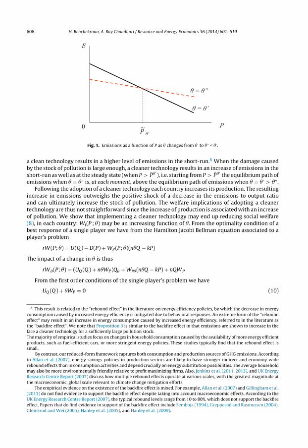
606 H. Benchekroun, A. Ray Chaudhuri / Resource and Energy Economics 36 (2014) 601–619

θ = θ”

P0

E

θ = θ’

P θ’~

Fig. 1. Emissions as a function of P as � changes from �′ to �′′ < �′ .

a clean technology results in a higher level of emissions in the short-run.8 When the damage causedby the stock of pollution is large enough, a cleaner technology results in an increase of emissions in theshort-run as well as at the steady state (when P > P�′

), i.e. starting from P > P�′the equilibrium path of

emissions when � = �′′ is, at each moment, above the equilibrium path of emissions when � = �′ > �′′.Following the adoption of a cleaner technology each country increases its production. The resulting

increase in emissions outweighs the positive shock of a decrease in the emissions to output ratioand can ultimately increase the stock of pollution. The welfare implications of adopting a cleanertechnology are thus not straightforward since the increase of production is associated with an increaseof pollution. We show that implementing a cleaner technology may end up reducing social welfare(8), in each country: Wi(P ; �) may be an increasing function of �. From the optimality condition of abest response of a single player we have from the Hamilton Jacobi Bellman equation associated to aplayer’s problem

rW(P; �) = U(Q ) − D(P) + WP(P; �)(n�Q − kP)

The impact of a change in � is thus

rW�(P; �) = (UQ (Q ) + n�WP)Q� + WP�(n�Q − kP) + nQWP

From the first order conditions of the single player’s problem we have

UQ (Q ) + �WP = 0 (10)

8 This result is related to the “rebound effect” in the literature on energy efficiency policies, by which the decrease in energyconsumption caused by increased energy efficiency is mitigated due to behavioral responses. An extreme form of the “reboundeffect” may result in an increase in energy consumption caused by increased energy efficiency, referred to in the literature asthe “backfire effect”. We note that Proposition 3 is similar to the backfire effect in that emissions are shown to increase in theface a cleaner technology for a sufficiently large pollution stock.The majority of empirical studies focus on changes in household consumption caused by the availability of more energy efficientproducts, such as fuel-efficient cars, or more stringent energy policies. These studies typically find that the rebound effect issmall.

By contrast, our reduced-form framework captures both consumption and production sources of GHG emissions. Accordingto Allan et al. (2007), energy savings policies in production sectors are likely to have stronger indirect and economy-widerebound effects than in consumption activities and depend crucially on energy substitution possibilities. The average householdmay also be more environmentally friendly relative to profit maximizing firms. Also, Jenkins et al. (2011, 2013), and UK EnergyResearch Centre Report (2007) discuss how multiple rebound effects operate at various scales, with the greatest magnitude atthe macroeconomic, global scale relevant to climate change mitigation efforts.

The empirical evidence on the existence of the backfire effect is mixed. For example, Allan et al. (2007) and Gillingham et al.(2013) do not find evidence to support the backfire effect despite taking into account macroeconomic effects. According to theUK Energy Research Centre Report (2007), the typical rebound levels range from 10 to 80%, which does not support the backfireeffect. Papers that do find evidence in support of the backfire effect include Semboja (1994), Grepperud and Rasmussen (2004),Glomsrod and Wei (2005), Hanley et al. (2005), and Hanley et al. (2009).

H. Benchekroun, A. Ray Chaudhuri / Resource and Energy Economics 36 (2014) 601–619 607

and thus

rW�(P; �) = (n − 1)�WPQ� + WP�(n�Q − kP) + nQWP (11)

We evaluate W� at P = PSS(�)

rW� |P=PSS(�) = (n − 1)�WPQ� + nQWP

which gives

rW� |P=PSS(�) = (n − 1)(�Q� + Q )WP + QWP

or

rW� |P=PSS(�) = (n − 1)E�WP + QWP (12)

When production remains unchanged, for an infinitesimal decrease in � there is a decrease ofemissions by Q which results in an increase of welfare since WP < 0. Thus, the second term of theright hand side of rW� |P=PSS(�) is negative and reflects the positive impact of a decrease in � due thereduction of the country’s own emissions if production is left unchanged. The first term of the righthand side reflects the impact on a country of the reaction of the other n − 1 countries to the change in�. If the decrease in � results in a decrease of emissions then the first term is negative and the impactof a clean technology on welfare is unambiguously positive. However, if E� < 0, then the sign of W�

can be positive or negative depending on the parameter values. We show below that W� may wellbe positive. The expression of W� is too cumbersome to allow a determination of the sign of W� forall parameter values. In this section, we show analytically, in a limit case (i.e. when the damage frompollution is large enough), that W� is positive: a decrease of the emissions per output ratio reduceswelfare. In the next section, we investigate the sign of W� numerically using plausible values of theparameters and show that there exist a range of realistic values of the parameters under which W� ispositive. We would like to note that the sign of W�(P) allows us to determine the impact of a (small)change of � on welfare at a given stock of pollution. It incorporates the change in welfare throughoutthe transition phase from an initial stock P to the steady state.

Proposition 4. (Main Proposition) For any n > 1, there exists s > 0 such that W� |P=PSS(�) > 0 for all s > s.

Proof. See appendix.

The positive shock of a cleaner technology results in a more “aggressive” or “voracious” behavior ofcountries that exacerbates the efficiency loss due to the presence of the pollution externality. Theintuition behind this result is similar to the one behind the ‘voracity effect’ in Tornell and Lane (1999)and Long and Sorger (2006), obtained in the context of growth under weak or absent property rights.The main feature of the equilibrium that drives this ‘voracity’ effect is the fact that the non-cooperativeemissions strategies are downward sloping functions of the stock of pollution.9 Unlike static gamesor dynamic games where countries would choose emissions paths, when Markovian strategies areconsidered to construct a Nash equilibrium, a country can still influence its rival’s action path eventhough it is taking its rival’s strategy as given. When the rival’s emission strategy is a downward slopingfunction of the stock of pollution, the action of increasing one’s emissions bears an additional benefit:increase in one’s emissions would result ceteris paribus in a larger level of the stock of pollutionwhich would in turn induce one’s rival to reduce her emissions. This possibility to influence rival’semissions’ path results in an overall more polluted world than would prevail if each country takesthe rival’s actions as given. The response of each country to a positive shock such as a reduction ofthe emissions to output ratio can be to expand its output. In this ‘aggressive’ setup, the extent of

9 This feature is related to the notion of intertemporal strategic substitutability at the steady state of the MPNE, used in Junand Vives (2004) which provides a taxonomy for possible strategic interactions in continuous-time dynamic duopoly models.Unlike the duopoly games covered in Jun and Vives (2004), in our model there is one state variable. Intertemporal strategicsubstitutability at the steady state of the MPNE, corresponds to a situation where an increase in the state variable of one firmdecreases the action of its rival.

608 H. Benchekroun, A. Ray Chaudhuri / Resource and Energy Economics 36 (2014) 601–619

the increase in output is such that the increase in pollution that follows and the damage it createsoutweigh the benefits from the additional consumption.

Remark 1. The Main Proposition’s content mirrors the comparative static result in oligopoly theorythat an increase in firms’ costs may end-up increasing firms’ profits (see Seade, 1983; Dixit, 1986).In our framework, countries’ instantaneous payoffs do not depend on each other’s flows of emissionsdirectly; they are interrelated through the damage from the stock of pollution, a stock to which theyall contribute. A decrease of the emissions per output ratio is analogous to a decrease in the damagefrom the production of a unit of output. However in our context, the dynamic dimension, an essentialfeature of a climate change model, brings an additional level of interaction between players, comparedto a static or repeated game, that contributes to our result. Indeed, if one considers the simple caseof two countries and where the damage arises from the flow of the sum of pollution (i.e., if the costof pollution were (1/2)s(E1 + E2)2 instead of (1/2)sP2), it can easily be shown that a decrease of theemissions to output ratio is always welfare improving, for any arbitrarily large value of the damageparameter s, in sharp contrast with the Main Proposition. One can possibly retrieve the perverse effectof implementing a cleaner technology, present in the MPNE, in a static framework using a conjecturalvariations approach. Dockner (1992) considered a dynamic oligopoly in the presence of adjustmentcosts and has shown that any steady state subgame-perfect equilibrium of the dynamic game canbe viewed as a conjectural variations equilibrium of a corresponding static game.10 However, theanalysis of the full fledged differential game allows us to first capture the intertemporal nature of thepollution game under consideration, and second, to take into account the transition dynamics whendetermining the impact of a decrease in the emissions per output ratio.

Remark 2. We note that the sign of W� |P=PSS(�) is not, a priori, the same as the sign of dW(PSS(�))/d�which captures the impact of a change in � on the level of welfare at the steady state. For a smalldiscrete change of �, the sign of dW(PSS(�))/d� gives an indication of the comparison of two welfarelevels evaluated at two different (steady state) stocks of pollution. When (dPSS(�)/d�) < 0, we have thatW� |P=PSS(�) > 0 implies dW(PSS(�))/d� = W� |P=PSS(�) + W ′(PSS(�))(dPSS(�)/d�) > 0 since W′(PSS(�)) < 0.

Remark 3. We would like to emphasize that our Main Proposition is obtained when we have asimultaneous decrease in all countries’ �′s. If, within this context, we considered a decrease in �i onlywhile �j, j /= i remain unchanged, then country i’s welfare would increase in response.11

5. Numerical example: climate change

The results derived in the previous sections gain relevance in the current context of climate change.Can the development of clean technologies alleviate the consequences of failing to reach a global inter-national agreement over GHG emissions?12 There is increasing support in the academic literature forthe view that innovative technology will play a central role to resolve the climate change predica-ment. Barrett (2009) argues that to stabilize carbon concentration at levels that are compatible witha long-run goal of an increase of the earth’s temperature by 2 ◦C with respect to the pre-industrialera will require a ‘technological revolution’. Galiana and Green (2009) similarly predict that reducingcarbon emissions will require an energy-technology revolution and a global technology race.13

10 Dockner (1992) shows that, in the case of a differential game with linear demand and quadratic costs, that the dynamicconjectures consistent with closed-loop steady state equilibria are negative, constant and symmetric.

11 Although not the focus of this paper, if we were to analyze the scenario where individual countries endogenously decidewhether to unilaterally invest in cleaner technology, taking the technology of the other countries as given, a given countrywould undertake the investment as long as its benefits of a decrease in �i outweighed its private cost of reducing �i . Within thiscontext, it is indeed possible that countries have an incentive to invest in a decrease in �i if, for example, the cost of a reductionin �i is a quadratic increasing function of the decrease in �i and as long as country i’s marginal benefit from a marginal decreasein �i is positive. Papers that study investment in clean technologies with a stock pollutant include Fischer et al. (2004), Gerlaghet al. (2009), and Toman and Withagen (2000).

12 Large polluters, such as the US, remained outside the Kyoto Protocol. Efforts to reach a post-Kyoto agreement have beendisappointing thus far, as is evident from the outcomes of the UN Climate Conferences (for example, at recent UNFCCC COPMeetings at Copenhagen (2009), Cancun (2010) and Doha (2012)).

13 Barrett (2006) argues that even treaties on the development of breakthrough technologies will typically share the same fateas treaties on emissions control since, unless technological breakthroughs exhibit increasing returns to scale. These treaties will

H. Benchekroun, A. Ray Chaudhuri / Resource and Energy Economics 36 (2014) 601–619 609

In this section, we investigate the sign of W� numerically, using ‘plausible’ values of the parametersbased on empirical evidence. We also present the effect of non-marginal changes in the emissions peroutput parameter on equilibrium welfare.

We would like to emphasize the absence of consensus in the literature about precise values ofthe parameters of the model. This is partly due to the large uncertainty surrounding the economicrepercussions of climate change. After a brief description of the ranges within which each parametermay fall, we start by presenting the impact of a change in the emissions per output ratio in a benchmarkcase and then conduct sensitivity analysis with respect to parameter values.

The value of the discount rate is the subject of important debates: The Stern Review uses 1.4%,Nordhaus uses 3–4%, others view discounting as unethical and argue that the rate of discount should benil (Heal, 2009). Most Integrated Assessment Models (IAMs) (for example, the DICE model (Nordhaus,1994), the RICE model (Nordhaus and Yang, 1996), the ENTICE model (Popp, 2003)) could have up to20 regions but usually consider between 8 and 15 regions. Following Nordhaus (1994), Hoel and Karp(2001) among others, we use the natural rate of decay k = 0.005.

As for the damage function, it is assumed that the damage is caused by the increase in CO2 con-centration with respect to its the pre-industrial era: P measures the difference between the currentstock of CO2 and the pre-industrial level of stock of CO2, assumed to be 590GtC (see e.g., Athanassoglouand Xepapadeas, 2012). The damage parameter is derived from estimates of the damage caused bya doubling of the stock of GHG: P = 590GtC. Let x denote the percentage of world GDP lost due to achange in temperature if the stock of pollution doubles relative to the current level. We have

x(WorldGDP) = nD(P)

Substituting for D(P), as given by (5), allows us to obtain s = 2(x(World GDP)/nP2).14 The value of x isundoubtedly the subject of heated debates on the political and academic arena and is crucial to definethe extent and the pace at which climate change related policies need to be implemented. In a recentstudy, Tol (2009) conducts the difficult task of aggregating the results of 14 studies on climate change’seconomic repercussions and gives a relationship between the increase of temperature and the damageusing different scenarios. The upper bound of the 95% confidence interval of x is approximately 10%under the assumption that temperature would rise by 2.5 ◦C and 12.5% if the temperature increases by3 ◦C.15 Based on experts’ opinions reported in Nordhaus (1994), Karp and Zhang (2012) use 21% as themaximum value for x. As Tol (2009) points out, most of the studies do not give any estimation of x forchanges in temperature that exceed 3 ◦C, do not look at a time horizon beyond 2100 and their estimatestypically ignore important non-market impacts such as extreme climate scenarios, biodiversity lossor political violence due to the increasing scarcity of resources induced by climate change. Taking intoaccount market and non-market impacts, Heal (2009) estimates that the cost could be 10% of worldincome. Taking into account the risk of catastrophe, the Stern Review estimates the 95th percentileto be 35.2% loss in global per-capita GDP by 2200. Thus, although for example the Stern Review uses5% as an estimate of x, it considers it as a conservative estimate. We will use 2.5% in the benchmarkcase, and conduct a sensitivity analysis with respect to x, using x = 5% and x = 10%.

We start by describing the benchmark case with the following parameter values, as summarizedby Table 1.

We also present the results for x = 0.05 and x = 0.1, holding the other parameter values constantat the benchmark levels. We also allow k to vary from 0 to ∞, holding the other parameter valuesconstant at the benchmark levels, and allow r to vary from 0 to ∞, holding the other parameter valuesconstant at the benchmark levels.16

fail because of the incentive of countries to free ride. However Hoel and de Zeeuw (2010) show that this pessimistic outcomecan be overturned if one takes into account that the adoption costs of a breakthough technology vary with the level of R&D.They show that a large coalition can be both stable and result in a significant welfare improvement.

14 List and Mason (2001) and Karp and Zhang (2012) have used the same approach to derive the numerical value of thepollution damage parameter. We note that this numerical simulation determines the impact of a reduction in � on the presentvalue of GDP net of damages.

15 In Nordhaus (1994) the 95% confidence interval of x is (− 30.0, 0) under the assumption that temperature rises by 3 ◦C.16 Note that r refers to the social discount rate which includes the rate of time preference.

610 H. Benchekroun, A. Ray Chaudhuri / Resource and Energy Economics 36 (2014) 601–619

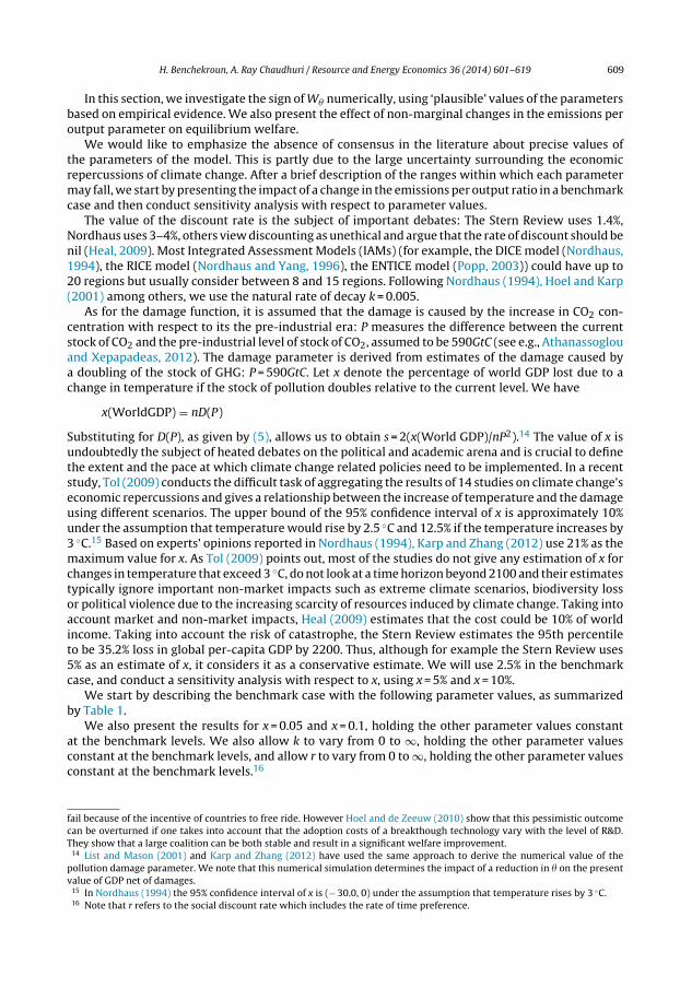
Table 1Parameter values.

Parameter Benchmark case

x 0.025n 10k 0.005r 0.025

0

G

θ3. 8315x10⁻⁴1.722x10⁻⁴

x = 2.5%

x = 10 %

x = 5%

Fig. 2. G at P = PSS(�0) as a function of �.

We define the function

G(P, �, �0) = W(P; �)|� − W(P; �)|�=�0

W(P; �)|�=�0

which represents the relative change in welfare as � changes from �0 to � and the stock of pollution isP.

In order to determine the value of �0 we use the following 2008 data. We use $60,689.812 billionas the value of the world GDP in 2008, as reported by the World Economic Outlook (2009) of theInternational Monetary Fund. We use 9.9 ± 0.9GtC as the value of total CO2 emission from fossil fuelcombustion and land use change in 2008, as reported by Le Quéré et al. (2009). We use a short-termdecay rate of emissions of 36% (i.e. 64% of emissions adds to the stock in any given year), as reportedby Newell and Pizer (2003). Also, 3.67 represents the conversion rate from units of carbon to units ofCO2. Using these values, we obtain

�0 = (9900 × 109)(3.67)(0.64)

60689 × 109= 3.831 5 × 10−4tCO2/$

We plot in Fig. 2, G(PSS(�0), �, �0) where �0 is set to 0.38315 kg of CO2/$ of GDP.17

We set B = �20 so that when � = �0 we retrieve the same specification of the linear quadratic models

of transboundary pollution where instantaneous utility U is expressed in terms of emissions (e.g.,Dockner and Long, 1993; Van der Ploeg and de Zeeuw, 1992; List and Mason, 2001; Hoel and Karp,2001).

We can observe that a decrease of the emissions per output from �0 can result in a loss in wel-fare: the welfare loss from the increase in pollution emissions outweighs the welfare gains from an

17 We note that there is ongoing debate about the value of the short term decay rate. The value of �0 may be higher, corre-sponding to a lower short term decay rate in line with Archer (2005) and Le Quéré et al. (2009) who discuss that carbon sinksare shrinking.

H. Benchekroun, A. Ray Chaudhuri / Resource and Energy Economics 36 (2014) 601–619 611

increase in consumption. Note that in Fig. 2, W(P; �)|�=�0< 0 and therefore when G(P, �, �0) > 0 we

have W(P; �)|� − W(P; �)|�=�0< 0.

The benchmark case represents a relatively optimistic scenario in terms of the damage of pollution.The sensitivity analysis that follows demonstrates that the consideration of less optimistic parametervalues strengthens the perverse effect that follows a reduction in the emissions per output ratio.

The emissions per output ratio has to decrease below �0 = 1.722 × 10−4tCO2/$ (i.e., a decrease of54. 33%) for the decrease to be welfare enhancing. The threshold �0 falls to 1.0155× 10−4tCO2/$ (i.e.,a decrease of 73.5%) when we use x = 5% and to 6.251×10−5tCO2/$ (i.e., a decrease of 83.68%) whenx = 10%.

We plot W� |P=PSS(�0) as a function of x (Fig. 3).

x0

W θ |P = P (θ )

0.5

0SS

0.001

Fig. 3. W� |P=PSS (�0) as a function of x.

For the benchmark case, for all x> 0.1 % we have W� |P=PSS(�0) > 0. A marginal decrease in emissionsper output ratio reduces welfare. The relationship of W� |P=PSS(�0) with respect to x (which is a proxyfor s) mirrors the result obtained analytically for the behavior of W� |P=PSS(�) in the limit case wheres→ ∞. The larger the damage parameter, the more likely a decrease of the emissions per output ratiowill be welfare reducing.

Let Z ≡ P0/PSS(�0). That is, Z is a parameter that sets the initial level of the stock of pollution relativeto the steady state stock of pollution. Fig. 4 shows that the graph of W� |P=Z∗PSS(�0) is a strictly increasingfunction of Z.

W θ |P = Z * P (θ )SS

Z0 0.263

0

0.231

x = 2.5 %

x = 10 %

Fig. 4. W� |P=Z∗PSS (�0) as a function of Z.

612 H. Benchekroun, A. Ray Chaudhuri / Resource and Energy Economics 36 (2014) 601–619

Fig. 4 shows that W� |P=Z∗PSS(�0) is positive for Z > Z = 0.263. The larger the stock of pollution atwhich we introduce a cleaner technology the more likely this will result in a welfare loss. The valueof Z decreases to 0.237 when x = 5% and to 0.231 when x = 10%.

Similarly, one can show that W� |P=PSS(�0) is a strictly decreasing function of k and is positive for

k < k = 0.025. The smaller the rate of decay, the more likely the implementation of a clean technologycan reduce all players’ welfare. The threshold k increases to 0.033 when x = 5% and to 0.039 whenx = 10%.

These results represent rather pessimistic conclusions about the ability of technology to alleviatethe tragedy of the commons, since it is when the damage is important and/or the stock of pollution islarge enough, and nature is least able to absorb pollution, that a decrease of the emissions per outputratio is mitigated by the increase in pollution emissions of each player to the point where welfarediminishes.

Moreover, it can be shown that W� |P=PSS(�0) > 0 for r > 0.00284. This is because the less forward-looking each country, the more aggressive the behavior of each player in terms of their emissionstrategies. Therefore, the higher is r, the greater the incentive of each country to increase emissionswhen faced with a cleaner technology.18

This numerical example has demonstrated that the perverse effect of implementing a cleaner tech-nology is not a mere theoretical possibility within the context of climate change. It is shown to be strongfor a significant and empirically relevant range of parameters. It is when the damage is relatively largeand/or the initial stock of pollution are relatively large and when the natural rate of decay of pollutionis relatively ‘small’, i.e. precisely the situations where the tragedy of the commons is at its worse, thatthe perverse effect prevails.

Moreover, a direct implication of the example is that a more rigorous pricing of carbon will notonly give the proper incentives to initiate a R&D race and the technology ‘revolution’ necessary tocontrol green house gas emissions, as argued, for instance, in Barrett (2009) and Galiana and Green(2009), but it is also necessary to prevent the implementation of the innovations from exacerbatingthe climate change problem.

6. Transfer of clean technologies

Consider now the case of an asymmetric pollution game where countries differ with respect totheir emissions per output ratios: we no longer assume that �i = �j for i, j = 1, . . ., n. The analysis ofthe previous sections can be reproduced. However, since the intuition of these results obtained in thesections above carry over to this case, we refrain from doing so and just give the description of theresults.

For simplicity consider the case of two groups of countries: �i = �l with i = 1, . . ., nC and �i = �h > �lwith i = nC + 1, . . ., n. Countries are identical in all respects except for the emissions per output ratios.Clearly, if nC/n is small enough then, any transfer of clean technologies from the group of clean countriesto the group of dirty countries, captured by a decrease in �h can lead to an increase of the dirty countries’emissions and a smaller welfare worldwide.

This possibility can also be shown to arise by considering the limit case where: �l = 0. In that case,the group of clean countries cannot condition their action on the stock of pollution even though theyare impacted by it. Each clean country chooses to produce at a rate A. The objective of each of the‘dirty’ countries’ governments is to choose a production strategy, Qi(t) (or equivalently a pollutioncontrol strategy), that maximizes the discounted stream of net benefits from consumption subject tothe accumulation equation

P(t) = �ni=nC +1εi(t) − kP(t) (13)

and the initial condition (3).

18 We note the role played by r depends on the value of �0. If, for example, we use 4.7× 10−4tCO2/$, instead of3.831 5×10−4tCO2/$, then it is possible that a marginally cleaner technology reduces equilibrium welfare only if r is sufficientlylow. This is because the role of r is complex when Markovian strategies are considered.

H. Benchekroun, A. Ray Chaudhuri / Resource and Energy Economics 36 (2014) 601–619 613

Clearly, if technology were fully transferable we would have a decrease of the dirty countries’emissions per output ratio from �h to 0 and therefore a transfer of technology results in a decrease ofemissions and an increase in all countries’ welfare. However, technologies are typically only partiallytransferable and the case �l = 0 is considered here only for an illustration.

Even though this is an asymmetric differential game, it is still analytically tractable and one canfollow identical steps used in the sections above to show that a decrease in �h may result in an increasein emissions of pollution, therefore reducing the clean countries’ welfare. Moreover, if the increasein emissions is large enough, this may result in all countries’ welfare diminishing following a ‘partial’transfer of clean technologies to the dirty countries.

7. Concluding remarks

This paper shows that the failure of coordination over emissions of transboundary pollutants mayprevent the international community from reaping any benefit from the creation and adoption of acleaner technology and may even result in exacerbating the tragedy of the commons.

The decrease of the emissions per output ratio has two components, the direct effect which is adecrease of emissions if the quantity produced by each player remains unchanged, and the indirecteffect since quantity produced changes and so do the emissions. Emissions may increase following theadoption of a cleaner technology, and the resulting increase in pollution damages can be substantialenough to annihilate the positive impact of the direct effect on welfare. We have shown that this mayarise for a wide range of ‘realistic’ values of the parameters of the model. Moreover, the possibilitythat emissions per output ratio and world emissions can evolve in opposite directions is supportedby recent anecdotal evidence within the context of climate change. While the world’s emissions peroutput ratio decreased from 0.54 (kilograms of CO2 per 1$ of GDP (PPP)) in 1990, to 0.50 in 2000and 0.47 in 2007, world’s emissions of CO2 increased from 21,899 millions of metric tons in 1990to 24,043 in 2000 and 29,595 in 2007 (see The Millennium Development Goals Report 2010 (UnitedNations)).

The results of this paper should not be interpreted as supporting the use of dirtier technologies.The main policy recommendation is that the efforts of discovering and using clean technologiesshould not be viewed as a substitute for the need to succeed in a multilateral coordination ofemissions.

The effort of creating clean technologies and the effort of coordinating the control over emissionsshould be pursued jointly. Intuition would suggest that the potential negative impact of clean tech-nologies would not take place if the adoption of a clean technology were accompanied with a welldesigned limit over emissions. Although this is intuitive, this idea deserves to be carefully studied sincethe impact of quotas in dynamic games are far from trivial (see, e.g., Dockner and Haug, 1990, 1991),as is the impact of cleaner technologies on the size of stable international environmental agreementsand the level of emissions control that can be self-enforced in such agreements (see Benchekroun andRay Chaudhuri, 2013).

Our analysis shows that the international cooperation over emissions control is not only neededas an incentive to induce R&D and innovation, but is also necessary to ensure that the development ofcleaner technologies does not exacerbate the free riding behavior that is at the origin of the climatechange problem. We have considered the impact of an exogenous change in the emissions per outputratio. The results of this paper suggest that the analysis of a model that embeds this framework andwhere investment in R&D to reduce emissions per output is taken into account, can be a promisingline of future research.

Acknowledgements

We are very grateful to Pablo Andrés Domenech, Isabel Galiana, Gérard Gaudet, Ngo Van Long andtwo anonymous referees for helpful comments and discussions. Usual disclaimers apply. We thankSSHRC, Hassan Benchekroun thanks FQRSC, and Amrita Ray Chaudhuri thanks the Board of Regents ofthe University of Winnipeg for financial support.

614 H. Benchekroun, A. Ray Chaudhuri / Resource and Energy Economics 36 (2014) 601–619

Appendix A. Proof of Proposition 1

We use the undetermined coefficient technique (see Dockner et al. (2000), Chapter 4) to derive thelinear Markov perfect equilibrium. The details are omitted. (See Proposition 1 of Dockner and Long(1993) for the case where � = 1) �

Appendix B. Derivation of (14)

In order to prove Proposition 2, it will be useful to rewrite the equilibrium production strategy as

Q (P; �) = 12n − 1

((n − 1 + 2n

k + r

� + r

)A − 1

�

� − 2k − r

2P

)(14)

where

� ≡√

(2k + r)2 + (2n − 1)4s�2.

The equilibrium production strategy is

Q = A − An˛�2

k + r + (2n − 1)˛�2− ˛�2

�P (15)

where

�2 = −2k − r +

√(2k + r)2 + (2n − 1)4s�2

2(2n − 1)

Thus,

˛�2 = � − 2k − r

2(2n − 1). (16)

Substituting (16) into the equilibrium production strategy and simplifying gives (14).

Appendix C. Proof of Proposition 2

We now evaluate dPSS/d�. The steady state is determined as the solution to

An − 1

2n − 1+ 2A

n

(2n − 1)k + r

� + r=

(k

n�+ 1

�

� − 2k − r

2(2n − 1)

)P (17)

which after simplification yields

A(

n − 1 + 2nk + r

� + r

)� =

(n� − nr + 2k(n − 1)

2n

)P (18)

Taking the derivative with respect to � and multiplying each side by (n� − nr + 2k(n − 1))/2n and using(18) gives

A(

n − 1 + 2nk + r

� + r

)(n� − nr + 2k(n − 1)

2n

)

+A

(−2n

k + r

(� + r)2

) (n� − nr + 2k(n − 1)

2n

)���

= 12

A(

n − 1 + 2nk + r

� + r

)��� +

(n� − nr + 2k(n − 1)

2n

)2

P�

(19)

where P� ≡ dPSS/d�.

H. Benchekroun, A. Ray Chaudhuri / Resource and Energy Economics 36 (2014) 601–619 615

Using the fact that

��� = �2 − (2k + r)2

�= � − (2k + r)2

�(20)

gives (n� − nr + 2k(n − 1)

2n

)2

P�

= A(

n − 1 + 2nk + r

� + r

)(n� − nr + 2k(n − 1)

2n

)+

A

(−2n

k + r

(� + r)2

n� − nr + 2k(n − 1)2n

− 12

(n − 1 + 2n

k + r

� + r

))�2 − (2k + r)2

�

When �→ ∞, we have

lim�→∞

⎛⎜⎝

A

(n − 1 + 2n

k + r

� + r

)(n� − nr + 2k(n − 1)

2n

)

+A

(−2n

k + r

(� + r)2

n� − nr + 2k(n − 1)2n

− 12

(n − 1 + 2n

k + r

� + r

))�2 − (2k + r)2

�

⎞⎟⎠

= − 12

A2k(2n − 1) + (3n − 1)nr

n< 0

(21)

Given the definition of �, we have the following:

lims→∞

dPSS

d�< 0, lim

k→∞dPSS

d�< 0, lim

r→∞dPSS

d�< 0, lim

n→∞dPSS

d�< 0�

Appendix D. Proof of Proposition 3

We have

E�(P; �) = 12n − 1

(n − 1 + 2n

k + r

� + r− 2n

k + r

(� + r)2���

)A − 1

2n − 1��

2P

From (20), we have that

E�(P; �) = E�(0; �) − 12n − 1

12�

(� − (2k + r)2

�

)P

with

E�(0; �) = 12n − 1

(n − 1 + 2n

k + r

� + r− 2n

k + r

(� + r)2

(� − (2k + r)2

�

))A.

Thus, we have

E�(P; �) < 0

iff

2(2n − 1)�E�(0; �)

� − ((2k + r)2/�)= P < P.

After simplification of E�(0 ; �) we have

E�(0; �) = 12n − 1

(n − 1 + 2nr

(k + r)

(� + r)2

(1 + (2k + r)2

�r

))A > 0 (22)

It follows that P > 0.

616 H. Benchekroun, A. Ray Chaudhuri / Resource and Energy Economics 36 (2014) 601–619

We now compare P to P. We have

P = 2�(n − 1 + 2n((k + r)/(� + r)))A� − 2k − r

and thus

P

P= 2(2n − 1)�E�(0; �)

� − ((2k + r)2/�)

� − 2k − r

2�(n − 1 + 2n((k + r)/(� + r)))A

or

P

P= �

(� + 2k + r)(2n − 1)E�(0; �)

(n − 1 + 2n((k + r)/(� + r)))A.

After simplification and substitution of E�(0 ; �) we have

(2n − 1)E�(0; �)(n − 1 + 2n((k + r)/(� + r))A

= (n − 1 + 2n((k + r)/(� + r)) − 2n((k + r)/((� + r)2))(� − ((2k + r)2)/�)n − 1 + 2n((k + r)/(� + r))

or

(2n − 1)E�(0; �)(n − 1 + 2n((k + r)/(� + r))A

= 1 − 2n(k + r)/(� + r)2(� − ((2k + r)2/�))n − 1 + 2n((k + r)/(� + r))

< 1

implying

P

P< 1�

Appendix E. Proof of Proposition 4: Main Proposition

For an analytical analysis of the sign of W� |P=PSS(�) rewrite

rW� |P=PSS(�) = (n − 1)�WPQ� + nQWP

as

rW� |P=PSS(�) =(

�Q�

Q+ n

n − 1

)(n − 1)QWP (23)

Recall that the equilibrium production strategy is given by

Q = 12n − 1

((n − 1 + 2n

k + r

� + r

)A − 1

�

� − 2k − r

2P

)(24)

Taking the derivative of Q with respect to � gives

Q� = −2An

(2n − 1)k + r

(� + r)2�� + 1

�2

� − 2k − r

2(2n − 1)P − 1

�

��

2(2n − 1)P (25)

Evaluating Q�Q at the steady state (that is, at P = PSS), where Q = kPSS/n�, gives

Q�

Q= −2A

n

(2n − 1)k + r

(� + r)2��

n�

kPSS+ 1

�

n

2(2n − 1)k(� − 2k − r − ���) (26)

which after using (20) and the fact that

lims→∞

� = ∞ (27)

H. Benchekroun, A. Ray Chaudhuri / Resource and Energy Economics 36 (2014) 601–619 617

gives

lims→∞

(1�

n

2(2n − 1)k(� − 2k − r − ���)

)= 1

�

n

2(2n − 1)k(−2k − r)

and, therefore,

lims→∞

(�Q�

Q

)= lim

s→∞

(−2A

n

(2n − 1)k + r

(� + r)2��

n�2

kPSS

)− n

2(2n − 1)k(2k + r) (28)

To determine the above limit it is convenient to write the steady state stock of pollution as a function� instead of s. The steady state stock of pollution is the solution to (18), which can be rewritten as

A(

n − 1 + 2nk + r

� + r

)� =

(12

− nr − 2k(n − 1)2n�

)�P (29)

or,

�P = A(n − 1 + 2n((k + r)/(� + r)))�(1/2) − (nr − 2k(n − 1))/2n�

(30)

Therefore, we have

lim�→∞

�P = 2A(n − 1)�.

From (27), we have the following:

lims→∞

�PSS = 2�(n − 1)A (31)

Rewriting (28) as

lims→∞

(�Q�

Q

)= lim

s→∞

(−2A

n

(2n − 1)(k + r)

n�

k

�2

(� + r)2

���

�

1�PSS

)− n

2(2n − 1)k(2k + r)

and using (27), (31) and (20) gives

lims→∞

(�Q�

Q

)= −2A

n

(2n − 1)(k + r)

n�

k

12�(n − 1)A

− n

2(2n − 1)k(2k + r)

or,

lims→∞

(�Q�

Q

)= 1

2k

n(2k + r − 4kn − 3nr)2n2 − 3n + 1

This implies that

lims→∞

(�Q�

Q+ n

n − 1

)= − nr

2k

3n − 1(n − 1)(2n − 1)

< 0� (32)

References

Allan, G., Hanley, N., McGregor, P., Swales, K., Turner, K., 2007. The impact of increased efficiency in the industrial use of energy:a computable general equilibrium analysis for the United Kingdom. Energy Economics 29, 779–798.

Archer, D., 2005. Fate of fossil fuel CO2 in geologic time. Journal of Geophysical Research 110, C09S05.Athanassoglou, S., Xepapadeas, A., 2012. Pollution control with uncertain stock dynamics: when, and how, to be precautious.

Journal of Environmental Economics and Management 63 (3), 304–320.Barrett, S., 2009. The coming global climate-technology revolution. Journal of Economic Perspectives 23, 53–75.Barrett, S., 2006. Climate treaties and “breakthrough” technologies. American Economic Review 96 (2), 22–25.Benchekroun, H., Ray Chaudhuri, A., 2013. Cleaner technologies and the stability of international environ-

mental agreements. Journal of Public Economic Theory http://www.accessecon.com/pubs/JPET/tempPDF/JPET-12-00115 0 0 1732599 temp.pdf (forthcoming).

Dixit, A., 1986. Comparative statics for oligopoly. International Economic Review 27, 107–122.Dockner, E.J., 1992. A dynamic theory of conjectural variations. Journal of Industrial Economics 40, 377–395.Dockner, E., Haug, A.A., 1990. Tariffs and quotas under dynamic duopolistic competition. Journal of International Economics 29,

147–159.

618 H. Benchekroun, A. Ray Chaudhuri / Resource and Energy Economics 36 (2014) 601–619

Dockner, E., Haug, A.A., 1991. Closed-loop motive for voluntary export restraints. Canadian Journal of Economics 24,679–685.

Dockner, E.J., Jorgensen, S., Long, N.V., Sorger, G., 2000. Differential Games in Economics and Management Science. CambridgeUniversity Press, UK.

Dockner, E.J., Long, N.V., 1993. International pollution control: cooperative versus noncooperative strategies. Journal of Envi-ronmental Economics and Management 24, 13–29.

Dutta, P.K., Radner, R., 2006. Population growth and technological change in a global warming model. Economic Theory 29,251–270.

Fischer, C., Withagen, C., Toman, M., 2004. Optimal investment in clean production capacity. Environmental and ResourceEconomics 28, 325–345.

Galiana, I., Green, C., 2009. Let the technology race begin. Nature 462, 570–571.Gerlagh, R., 2011. Too much oil. CESifo Economic Studies 57, 79–102.Gerlagh, R., Kverndokk, S., Rosendahl, K.E., 2009. Optimal timing of climate change policy: interaction between carbon taxes

and innovation externalities. Environmental and Resource Economics 43, 369–390.Gillingham, K., Kotchen, M.J., Rapson, D.S., Wagner, G., 2013. Energy policy: the rebound effect is overplayed. Nature 493,

475–476.Glomsrod, S., Wei, T., 2005. Coal cleaning: a viable strategy for reduced carbon emissions and improved environment in China.

Energy Policy 33, 525–542.Greening, L.A., Greene, D.L., Difiglioc, C., 2000. Energy efficiency and consumption – the rebound effect – a survey. Energy Policy

28, 389–401.Grepperud, S., Rasmussen, I., 2004. A general equilibrium assessment of rebound effects. Energy Economics 26, 261–282.Hanley, N., McGregor, P., Swales, K., Turner, K., 2005. Do increases in resource productivity improve environmental quality?

Theory and evidence on rebound and backfire effects from an energy-economy-environment regional computable generalequilibrium model of Scotland. Working Paper. Department of Economics, University of Strathclyde.

Hanley, N., McGregor, P., Swales, K., Turner, K., 2009. Do increases in energy efficiency improve environmental quality andsustainability? Energy Economics 31, 648–666.

Heal, G., 2009. Climate economics: a meta-review and some suggestions for future research. Review of Environmental Economicsand Policy 3, 4–21.

Hoel, M., 2011. The green paradox and greenhouse gas reducing investments. International Review of Environmental andResource Economics 5, 353–379.

Hoel, M., de Zeeuw, A., 2010. Can a focus on breakthrough technologies improve the performance of international environmentalagreements? Environmental and Resource Economics 47, 395–406.

Hoel, M., Karp, L., 2001. Taxes and quotas for a stock pollutant with multiplicative uncertainty. Journal of Public Economics 82,91–114.

Jenkins, J., Nordhaus, T., Shellenberger, M., 2011. Energy emergence: rebound and backfire as emergent phenomena (Break-through Institute Report, 2011), Accessed at: http://thebreakthrough.org/archive/new report how efficiency can

Jenkins, J., Nordhaus, T., Shellenberger, M., 2013. Energy efficiency: beware of overpromises (Breakthrough Institute Report,2013), Accessed at: http://thebreakthrough.org/index.php/programs/energy-and-climate/the-limits-of-efficiency/

Jørgensen, S., Zaccour, G., 2001. Time consistent side payments in a dynamic game of downstream pollution. Journal of EconomicDynamics and Control 25 (12), 1973–1987.

Jørgensen, S., Martin-Herran, G., Zaccour, G., 2010. Dynamic games in the economics and management of pollution. Environ-mental Modeling and Assessment 15, 433–467.

Jun, B., Vives, X., 2004. Strategic incentives in dynamic duopoly. Journal of Economic Theory 116 (2), 249–281.Karp, L., Zhang, J., 2012. Taxes versus quantities for a stock pollutant with endogenous abatement costs and asymmetric

information. Economic Theory 49, 371–409.List, J., Mason, C., 2001. Optimal institutional arrangements for transboundary pollutants in a second-best world: evidence from

a differential game with asymmetric players. Journal of Environmental Economics and Management 42, 277–296.Long, N.V., Sorger, G., 2006. Insecure property rights and growth: the role of appropriation costs, wealth effects, and hetero-

geneity. Economic Theory 28, 513–529.Newell, R.G., Pizer, W.A., 2003. Regulating stock externalities under uncertainty. Journal of Environmental Economics and

Management 45, 416–432.Nordhaus, W., 1994. Managing the Global Commons: The Economics of the Greenhouse Effect. MIT Press, Cambridge, MA.Nordhaus, W.D., Yang, Z., 1996. A regional dynamic general-equilibrium model of alternative climate-change strategies. Amer-

ican Economic Review 86, 741–765.Van der Ploeg, F., Withagen, C., 2012. Is there really a green paradox? Journal of Environmental Economics and Management

64, 342–363.Van der Ploeg, F., de Zeeuw, A., 1992. International aspects of pollution control. Environmental and Resource Economics 2,

117–139.Popp, D., 2003. ENTICE: endogenous technological change in the DICE model of global warming. NBER Working Papers 9762.Quentin Grafton, R., Kompas, T., Long, N.V., 2012. Substitution between biofuels and fossil fuels: is there a green paradox?

Journal of Environmental Economics and Management 64, 328–341.Le Quéré, C., Raupach, M.R., Canadell, J.G., Marland, G., Bopp, L., Ciais, P., Conway, T.J., Doney, S.C., Feely, R.A., Foster, P., Friedling-

stein, P., Gurney, K., Houghton, R.A., House, J.I., Huntingford, C., Levy, P.E., Lomas, M.R., Majkut, J., Metzl, N., Ometto, J.P.,Peters, G.P., Prentice, I.C., Randerson, J.T., Running, S.W., Sarmiento, J.L., Schuster, U., Sitch, S., Takahashi, T., Viovy, N., Vander Werf, G.R., Woodward, F.I., 2009. Trends in the sources and sinks of carbon dioxide. Nature Geoscience 2, 831–836.

Seade, J.K., 1983. Price, profits and taxes in oligopoly. Working paper. University of Warwick.Semboja, H., 1994. The effects of an increase in energy efficiency on the Kenyan economy. Energy Policy 22, 217–225.Sinn, H.W., 2012. The Green Paradox: A Supply-side Approach to Global Warming. MIT Press, Cambridge.Sorrell, S., Dimitropoulos, J., 2008. The rebound effect: microeconomic definitions, limitations and extensions. Ecological Eco-

nomics 65, 636–649.

H. Benchekroun, A. Ray Chaudhuri / Resource and Energy Economics 36 (2014) 601–619 619

Tol, R.S.J., 2009. The economic effects of climate change. Journal of Economic Perspectives 23, 29–51.Toman, M.A., Withagen, C., 2000. Accumulative pollution, ‘clean technology’ and policy design. Resource and Energy Economics

22, 367–384.Tornell, A., Lane, P.R., 1999. The voracity effect. The American Economic Review 89 (1), 22–46.UK Energy Research Centre Report, 2007. The rebound effect: an assessment of the evidence for economy-wide energy savings

from improved energy efficiency.