trajectory planning for robot manipulators part 4 · the kinematic model is x= l 1c 1 +l 2c 12 y =...
TRANSCRIPT
Trajectory Planning for Robot Manipulators
Part 4
Claudio Melchiorri
Dipartimento di Elettronica, Informatica e Sistemistica (DEIS)
Universita di Bologna
email: [email protected]
C. Melchiorri (DEIS) Trajectory Planning 1 / 21
Workspace trajectories
Workspace trajectories
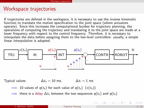
If trajectories are defined in the workspace, it is necessary to use the inverse kinematicfunction to translate the motion specification to the joint space (where actuatorsoperate). Since this increases the computational burden for trajectory planning, theoperations of computing the trajectory and translating it to the joint space are made at alower frequency with respect to the control frequency. Therefore, it is necessary tointerpolate the data before assigning them to the low-level controllers: usually, a simplelinear interpolation is adopted.
TRJ IK i CONTR ROBOT -- -
6
x(tn) q(tn) qr
-
INT- --q(tk)
Typical values: ∆tn = 10 ms, ∆tl = 1 ms
=⇒ 10 values of q(tk) for each value of q(tn) (x(tn))
=⇒ there is a delay ∆tn between the two sequences q(tk) and q(tn)
C. Melchiorri (DEIS) Trajectory Planning 2 / 21
Workspace trajectories
Workspace trajectories
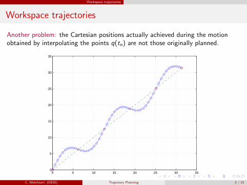
Another problem: the Cartesian positions actually achieved during the motionobtained by interpolating the points q(tn) are not those originally planned.
0 5 10 15 20 25 30 350
5
10
15
20
25
30
35
C. Melchiorri (DEIS) Trajectory Planning 3 / 21

Workspace trajectories
Workspace trajectories
For the computation of the workspace trajectories, it is possible to adopt one ofthe techniques used for the joint space (substituting the joint variable q(t) withx(t), i.e. a position or an orientation in the Cartesian space) or to defineanalytically the geometric path (e.g. an ellipse) as a function of time (i.e.p = p(t)) or, better, in a parametric form p = p(s), being s = s(t) a properparameterization defining the motion law.
C. Melchiorri (DEIS) Trajectory Planning 4 / 21
Workspace trajectories
Example: planar 2 dof manipulator
-1.5
-1
-0.5
0
0.5
1
1.5
-1.5 -1 -0.5 0 0.5 1 1.5
o
o
Traiettoria di manipolatore planare
o
o
o
o
o
o
o
o
o
o
o
o
o
o
o
o
o
o
o
o
o
o
o
o
o
o
o
o
o
o
o
o
o
o
o
o
o
o
o
o
o
o
o
o
o
o
o
o
o
o
o
o
o
o
o
o
o
o
o
o
o
o
o
o
o
o
o
o
o
o
o
o
o
o
o
o
o
o
o
o
o
o
o
o
o
o
o
o
o
o
o
o
o
o
o
o
o
o
o
o
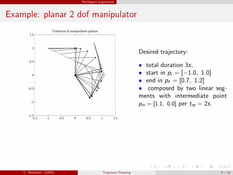
Desired trajectory:
• total duration 3s,• start in pi = [−1.0, 1.0]• end in pf = [0.7, 1.2]• composed by two linear seg-ments with intermediate pointpm = [1.1, 0.0] per tm = 2s.
C. Melchiorri (DEIS) Trajectory Planning 5 / 21

Workspace trajectories
Example: planar 2 dof manipulator
Consider the parametric form
x(t) = x0 +x1 − x0
∆Tτ
y(t) = y0 +y1 − y0
∆Tτ
where ∆T = t1 − t0, and τ ∈ [0,∆T ] is defined so that desired position/velocityprofiles are obtained, for example linear segments with parabolic blends (positionin the workspace). The kinematic model is
x = l1C1 + l2C12 y = l1S1 + l2S12
while the inverse kinematic equations are
C2 =x2 + y2 − a22 − a23
2a2a3S2 =
√
1− C 22
θ2 = atan2 (S2, C2) θ1 = atan2 (y , x)− atan2 (a2S2, a1 + a2C2)
C. Melchiorri (DEIS) Trajectory Planning 6 / 21
Workspace trajectories
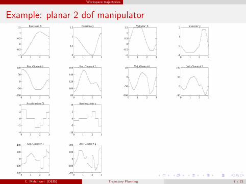
Example: planar 2 dof manipulator
-1
-0.5
0
0.5
1
1.5
0 1 2 3
Posizione X
0
0.5
1
1.5
0 1 2 3
Posizione y
-100
-50
0
50
100
0 1 2 3
Pos. Giunto # 1
80
100
120
140
160
0 1 2 3
Pos. Giunto # 2
-1
-0.5
0
0.5
1
1.5
0 1 2 3
Velocita‘ X
-1
0
1
2
0 1 2 3
Velocita‘ y
-100
-50
0
50
0 1 2 3
Vel. Giunto # 1
-50
0
50
100
0 1 2 3
Vel. Giunto # 2
-4
-2
0
2
4
0 1 2 3
Accelerazione X
-10
-5
0
5
10
0 1 2 3
Accelerazione y
-400
-200
0
200
400
0 1 2 3
Acc. Giunto # 1
-200
-100
0
100
200
0 1 2 3
Acc. Giunto # 2
C. Melchiorri (DEIS) Trajectory Planning 7 / 21

Workspace trajectories
Position trajectories
To plan a trajectory in the workspace, usually the geometric path p (line, circle,ellipse, . . . ) is defined as a function of a parameter s(t): p = p(s).
The parameter s = s(t) is computed by using one of the techniques discussed forjoint space trajectories. A classical approach is to plan s(t) as a linear functionwith parabolic blends, in order to have in the work space acceleration/decelerationtracts (low stress for the mechanical and actuation system).
Notice that for parameterized trajectories the following conditions hold:
p =d p
dss, p =
d p
dss +
d2 p
ds2s2
C. Melchiorri (DEIS) Trajectory Planning 8 / 21

Workspace trajectories
Position trajectories
Curvature of a geometric path
Consider a path Γ in the workspace IR3, expressed in parametric form
p = p(r) =
x(r)y(r)z(r)
, r ∈ [ra, rb]
Assume that the curve is regular, i.e.
p =d p
dr6= 0, ∀r ∈ [ra, rb]
Given a point pa of Γ, and a motion direction on the path, the arc lenght of ageneric point p(r) is defined as
s =
∫ p(r)
pa
||p(ρ)||dρ
C. Melchiorri (DEIS) Trajectory Planning 9 / 21
Workspace trajectories
Position trajectories
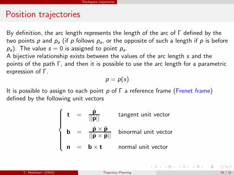
By definition, the arc length represents the length of the arc of Γ defined by thetwo points p and pa (if p follows pa, or the opposite of such a length if p is beforepa). The value s = 0 is assigned to point pa.A bijective relationship exists between the values of the arc length s and thepoints of the path Γ, and then it is possible to use the arc length for a parametricexpression of Γ.
p = p(s)
It is possible to assign to each point p of Γ a reference frame (Frenet frame)defined by the following unit vectors
t = p||p||
tangent unit vector
b =p× p
||p× p||binormal unit vector
n = b× t normal unit vector
C. Melchiorri (DEIS) Trajectory Planning 10 / 21

Workspace trajectories
Position trajectories
The unit vector t lies along the direction tangent to Γ in p, and is directedalong the positive s direction
The unit vector n defines, with t, the osculating plane O, defined as theplane containing point p and a point p′ ∈ Γ when p′ → p.
The unit vector b (binormal) is defined so that the frame (t, n, b) isright-handed. Notice that it is not always possible to define uniquely theFrenet frame.
C. Melchiorri (DEIS) Trajectory Planning 11 / 21

Workspace trajectories
Position trajectories
Segment of a line
The linear geometric path between points pi and pf has a parametricrepresentation expressed by
p(s) = pi +s
||pf − pi ||(pf − pi), s ∈ [0, ||pf − pi ||]
Moreover, by deriving p with respect to s, one obtains
d p
ds=
pf − pi
||pf − pi ||,
d2 p
ds2= 0
It is possible to plan a trajectory through a sequence of points with the samemodalities seen in the joint space. If it is required to pass exactly through theintermediate points, then it is possible to compute the parameter s using one ofthe motion laws defined in the joint space (e.g. cubic, trapezoidal, . . . ).In case it is not required for the manipulator to pass through the intermediatepoints, the geometric path can be defined for example by linear segments withpolynomial blends (position error, but non null velocity in the via points).
C. Melchiorri (DEIS) Trajectory Planning 12 / 21
Workspace trajectories
Position trajectories
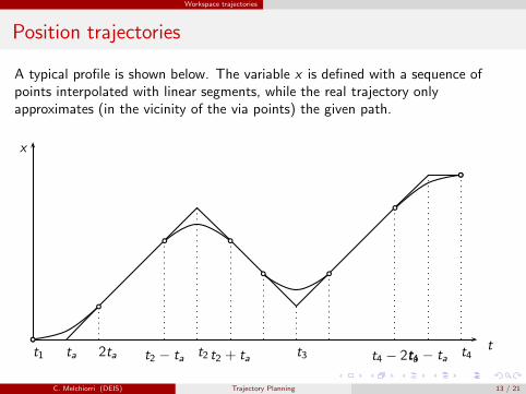
A typical profile is shown below. The variable x is defined with a sequence ofpoints interpolated with linear segments, while the real trajectory onlyapproximates (in the vicinity of the via points) the given path.
x
tt1 t2 t3 t4ta 2ta t2 − ta t2 + ta t4 − 2tat4 − ta
C. Melchiorri (DEIS) Trajectory Planning 13 / 21
Workspace trajectories
Position trajectories
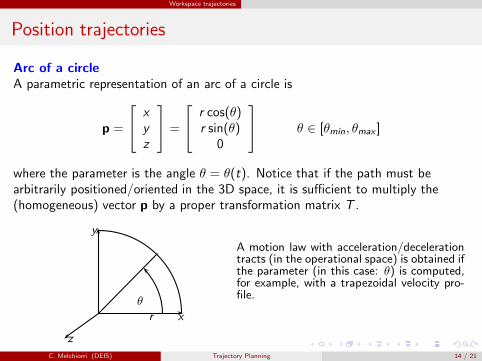
Arc of a circle
A parametric representation of an arc of a circle is
p =
x
y
z
=
r cos(θ)r sin(θ)
0
θ ∈ [θmin, θmax ]
where the parameter is the angle θ = θ(t). Notice that if the path must bearbitrarily positioned/oriented in the 3D space, it is sufficient to multiply the(homogeneous) vector p by a proper transformation matrix T .
y
x
z
θ
r
A motion law with acceleration/decelerationtracts (in the operational space) is obtained ifthe parameter (in this case: θ) is computed,for example, with a trapezoidal velocity pro-file.
C. Melchiorri (DEIS) Trajectory Planning 14 / 21

Workspace trajectories
Position trajectories - Example
Planar 2 dof manipulator with links’ lenght: a1 = a2 = 1. The desired circularmotion is defined by
center = [0.5, 0.5], radius r = 0.7θi = −60, θf = 90, T = 1 s
−1 −0.5 0 0.5 1 1.5 2−1
−0.5
0
0.5
1
1.5
2Traiettoria di manipolatore planare
0 0.1 0.2 0.3 0.4 0.5 0.6 0.7 0.8 0.9 1−0.2
0
0.2
0.4
0.6
0.8
1
1.2Traiettoria cartesiana x(t), y(t)
C. Melchiorri (DEIS) Trajectory Planning 15 / 21

Workspace trajectories
Position trajectories
0 0.1 0.2 0.3 0.4 0.5 0.6 0.7 0.8 0.9 1−0.2
0
0.2
0.4
0.6
0.8
1
1.2Traiettoria cartesiana x(t), y(t)
0 0.1 0.2 0.3 0.4 0.5 0.6 0.7 0.8 0.9 1−150
−100
−50
0
50
100
150Traiettorie di posizione giunto
C. Melchiorri (DEIS) Trajectory Planning 16 / 21

Workspace trajectories
Rotational trajectories
Planning trajectories in terms of changes in orientation is somehow more complexthan planning in position only. While it is quite simple to plan a motion betweenpoints pi and pf , the same is not true for interpolating the orientation betweentwo rotational matrices Ri and Rf : for example if the elements rij are changedlinearly from the initial (in Ri ) to the final (in Rf ) value, there is not guaranteethat the intermediate matrices are real rotation matrices (orthogonal columns withunit norm).
Usually, the Euler or RPY angles are employed or, alternatively, the angle/axisrepresentation.
With the Euler or RPY angles, two triples φi , φf are defined, and an interpolationbased on one of the presented techniques can be adopted (advisable in any casecontinuity at least of the in rotational velocity).
C. Melchiorri (DEIS) Trajectory Planning 17 / 21

Workspace trajectories
Rotational trajectories
With the angle/axis representation, if Ri and Rf are the initial and final rotationmatrices, then a matrix Ri ,f exists such that
Ri Ri ,f = Rf
or
Ri ,f = RTi Rf =
r11 r12 r13r21 r22 r23r31 r32 r33
Then, the unit vector w and the rotational angle θ are
θr = acosr11 + r22 + r33 − 1
2(1)
w =1
2 sin θr
r32 − r23r13 − r31r21 − r12
(2)
C. Melchiorri (DEIS) Trajectory Planning 18 / 21
Workspace trajectories
Rotational trajectories
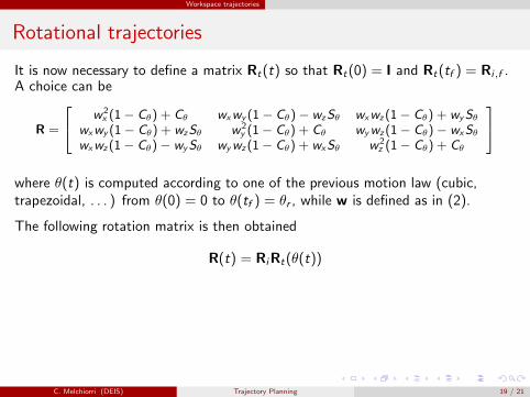
It is now necessary to define a matrix Rt(t) so that Rt(0) = I and Rt(tf ) = Ri ,f .A choice can be
R =
w2x (1− Cθ) + Cθ wxwy (1− Cθ)− wzSθ wxwz (1− Cθ) + wySθ
wxwy (1− Cθ) + wzSθ w2y (1− Cθ) + Cθ wywz (1− Cθ)− wxSθ
wxwz (1− Cθ)− wySθ wywz (1− Cθ) + wxSθ w2z (1− Cθ) + Cθ
where θ(t) is computed according to one of the previous motion law (cubic,trapezoidal, . . . ) from θ(0) = 0 to θ(tf ) = θr , while w is defined as in (2).
The following rotation matrix is then obtained
R(t) = RiRt(θ(t))
C. Melchiorri (DEIS) Trajectory Planning 19 / 21

Workspace trajectories
Workspace trajectories
Final considerations
Some techniques for planning trajectories in the joint and in the work space havebeen illustrated.
If the trajectory is planned in the work space, the end-effector moves along welldefined paths, a very important aspect in many industrial applications.
On the other hand, the computational burden is higher in case of work-spacetrajectories. For this reason, the frequency at which the trajectory in computed inlower than the control frequency, and an interpolation is then necessary.
Moreover, since the velocity/acceleration/torque limits required in the work-spacemay result non physically achievable in the joint space (i.e. in the actuationspace) a re-computation of the trajectory might be necessary.
C. Melchiorri (DEIS) Trajectory Planning 20 / 21

Workspace trajectories
Workspace trajectories
Final considerations
Finally, singular configurations may generate problems if the trajectory is plannedin the work space.
As a matter of fact, if a motion defined in the work space reaches points close tosingular configuration, it should be avoided. Therefore, the trajectory should bechecked in advance and, in case, not actuated or modified.
Clearly all these problems are not present if the trajectory is planned in the jointspace.
C. Melchiorri (DEIS) Trajectory Planning 21 / 21