train driver scheduling - university of leeds · air crew rostering. precise timing for drivers...
TRANSCRIPT
Train Drive r Scheduling
by
Ann Sau King Kwan
Submitted in accordance with the requirementsfor the degree of Doctor of Philosophy
The University of LeedsSchool of Computer Studies
August 1999
The candidate confirms that the work submitted is her own and that appropriate credithas been given where reference has been made to the work of others.

Acknowledgements
I would like to thank my supervisor, Professor A. Wren for his help, guidance and
encouragement. Most importantly, he gave me the opportunity to get re-started on
scheduling. I would like to thank Margaret Parker for her help and support throughout
these years. I would also like to thank the scheduling staff of GNER, Thameslink,
Northern Spirit and WAGN for providing us with the test data. Thanks are to the
Engineering and Physical Sciences Research Council for providing the research grants.
Finally, my thanks go to Raymond for his support and patience.

ii
Abstract
This thesis describes research into solving the U.K. train driver scheduling problems,
which are very complex compared to the bus or other public transport driver scheduling
problems. A set covering approach comprising a shift generation stage followed by a
shift selection stage is proposed. A review of existing computerised systems for solving
train driver scheduling and bus driver scheduling is presented, with a brief description of
air crew rostering.
Precise timing for drivers travelling as passengers in the train driver scheduling problem
is one of the crucial and complicated issues in producing operable driver schedules. This
problem has been resolved satisfactorily by a simplified search method specially
designed for a timetabled service network. The shift generation stage uses various
techniques and heuristics to generate legal shifts satisfying nearly all the constraints
present in the train problem. The shift generation process is combined with an integer
linear programme (ILP) solver originally used for bus driver scheduling. The new
system, TRACS II has been demonstrated to be successful for a wide variety of train
problems. Since the bus driver scheduling problem is a special case of the train problem,
TRACS II has also been used to solve some bus problems successfully.
There are some computational limitations in using an ILP method. A new approach
using a Genetic Algorithm is proposed for the shift selection stage. It aims to replace the
branch and bound process which sometimes fail to produce an integer solution. The
Genetic Algorithm approach involves identifying important combinatorial traits present
in the relaxed LP solution and makes use of them to limit the search space for the GA. It
involves using the information provided by the relaxed LP solution for the choice of
genes in the chromosome, and inheritance. The performance of the new GA process is
reported and the results compare favourably to those produced by the ILP in terms of
speed and ability to solve large problems.

iii
Contents
1 The Train Driver Scheduling Problem 1
1.1 Introduction ............................................................................................... 1
1.2 Train work ................................................................................................. 2
1.3 Problem description ................................................................................... 3
1.3.1 Non-wheel turning work ............................................................... 5
1.3.2 Train graphs ................................................................................... 6
1.3.3 Forming a train driver schedule .................................................... 7
1.4 Features of the train driver scheduling problem ........................................ 8
1.4.1 Route and traction knowledge ....................................................... 8
1.4.2 Multi-depots .................................................................................. 9
1.4.3 Driver travelling as passenger ....................................................... 9
1.4.4 Shifts containing work on many different units .......................... 11
1.4.5 Round the clock operation ........................................................... 11
1.4.6 Windows of relief opportunities .................................................. 12
1.5 Union agreements .................................................................................... 12
1.6 Bus driver scheduling problems – a special case of train driver scheduling
...................................................................................................... 14
1.6.1 Solving the bus driver scheduling problems using IMPACS ...... 14
1.6.2 Differences between train driver scheduling and bus driver
scheduling problems .................................................................... 14
1.7 Background of research ........................................................................... 15
1.8 Research approach ................................................................................... 17
1.8.1 GENERATION ........................................................................... 19
1.8.2 SELECTION ............................................................................... 20
1.9 Benefits of scheduling train drivers by computer ................................... 22
2 Literature review 25
2.1 Introduction ............................................................................................. 25
2.2 Computerised train driver scheduling systems ........................................ 26
2.2.1 British Rail .................................................................................. 26
2.2.2 The New Jersey Railway System ................................................ 26
iv
2.2.3 The Italian State Railways ........................................................... 28
2.2.4 The Dutch Railways .................................................................... 29
2.3 Bus crew scheduling systems .................................................................. 31
2.3.1 Heuristic Approaches ...................................................................32
2.3.1.1 The TRACS System .......................................................32
2.3.1.2 The COMPACS System .................................................33
2.3.1.3 The RUCUS-II System................................................... 34
2.3.1.4 The HASTUS System.................................................... 35
2.3.1.5 The HOT II System ....................................................... 37
2.3.1.6 The BDS System ............................................................38
2.3.1.7 A Lagrangean relaxation based heuristic ...................... 38
2.3.1.8 The MICROBUS System .............................................. 39
2.3.1.9 The Ravenna System ..................................................... 40
2.3.1.10 A Tabu Search approach ................................................40
2.3.1.11 Overview of the heuristic approach .............................. 42
2.3.2 Mathematical programming approach ........................................ 43
2.3.2.1 The IMPACS System .................................................... 43
2.3.2.2 The Crew-Opt method of HASTUS .............................. 45
2.3.2.3 The CRU-SCHED System .............................................47
2.3.2.4 The EXPRESS System .................................................. 47
2.3.2.5 Overview of the mathematical approach ....................... 49
2.4 Review of other approaches in solving driver scheduling problems ...... 50
2.5 Air crew rostering or pairing systems ..................................................... 52
3 The TRACS II driver scheduling system 54
3.1 Introduction ............................................................................................. 54
3.2 Outline of TRACS II ............................................................................... 55
3.2.1 TRACS II modules ...................................................................... 56
3.2.2 Input data files for TRACS II ...................................................... 57
3.2.3 The results from TRACS II ......................................................... 58
4 Drivers travelling as passengers 60
4.1 Introduction ............................................................................................. 60
4.2 Simple approaches for tackling passenger travel .................................... 63
4.2.1 Using estimated average travel time ........................................... 63
v
4.2.2 Adding artificial trips ...................................................................63
4.2.3 Using ‘nominated travel’ as in IMPACS .................................... 64
4.2.4 ‘Overlapping work’ as passenger travel ...................................... 65
4.3 Solving the passenger travel problem ..................................................... 67
4.3.1 Related work ............................................................................... 68
4.3.2 Earliest arrival times and latest departure times ......................... 69*
4.3.3 Information required and improving search efficiency .............. 71∗
4.3.4 Walking allowance and leeway .................................................. 73∗
4.3.5 Algorithms for computing passenger travel journeys ................ 74∗
4.3.5.1 Algorithm for finding feasible connections by trains ... 74∗
4.3.5.2 Making additional connections by walking ................. 78∗
4.4 Travel information produced from TRAVEL ......................................... 79
4.5 Running time of TRAVEL ...................................................................... 81
4.6 Comparison of results with early case studies ........................................ 82
4.7 Conclusion ............................................................................................... 83
5 Build ing potential shifts 85
5.1 Introduction ............................................................................................. 85
5.2 Outline of the shift generation process in IMPACS ................................ 86
5.2.1 An illustration of GEN forming two part shifts .......................... 87
5.2.2 Five types of shifts formed by GEN ............................................ 88
5.3 Difficulties of using GEN in the train situation ...................................... 89
5.4 New approach used in the shift generation process ............................... 91∗
5.4.1 Formation of spells ..................................................................... 92∗
5.4.2 Formation of stretches ................................................................ 93∗
5.4.2.1 Sieving process for stretches ........................................ 94∗
5.4.2.2 An illustration of forming stretches ............................. 96∗
5.4.3 Formation of shifts with at least one mealbreak ........................ 96∗
5.4.3.1 Sieving process one ...................................................... 98∗
5.4.3.2 Sieving process two .................................................... 100∗
5.4.4 Formation of shifts with no mealbreak in between the driving
work .......................................................................................... 101∗
5.4.5 Formation of split shifts .......................................................... 101∗ *
* These sections are withheld due to Intellectual Property Rights
vi
5.4.6 Specific requirements in train driver scheduling ...................... 102∗
5.4.6.1 Passenger travel .......................................................... 102∗
5.4.6.2 Route knowledge ........................................................ 102∗
5.4.6.3 Traction knowledge ..................................................... 104∗
5.4.6.4 Overnight work ........................................................... 105∗
5.4.6.5 Mealbreak (PNB) rules ................................................ 106∗
5.4.6.6 Other non-wheel turning work .................................... 108∗
5.4.6.7 Classifying shifts by spreadover range or signing on time
.................................................................................................... 109
5.5 Running time of the shift generation process ........................................ 110
5.6 Uncovered work .................................................................................... 110
5.7 Parallel building of shifts ...................................................................... 111
5.8 Refinement of the sets of potential shifts created by BUILD ............... 111
5.8.1 Reduction of the shift set – Program SIEVE ............................. 111
5.8.2 Combining different potential shift sets – Program MERGE ... 112
5.9 Shift selection using Integer Linear Programming – Process SCHEDULE
.................................................................................................... 113
5.10 Conclusions ........................................................................................... 113
6 Applications and implementation of TRACS II 114
6.1 Introduction ........................................................................................... 114
6.2 Application of TRACS II in the train situation ..................................... 115
6.2.1 Great North Eastern Railway (formerly InterCity East Coast) . 115
6.2.2 Thameslink ................................................................................ 117
6.2.3 London Underground ................................................................ 120
6.2.4 Northern Spirit (formerly Regional Railway North East) ......... 123
6.2.5 West Anglia and Great Northern (WAGN) ............................... 126
6.2.6 South Wales and West .............................................................. 128
6.2.7 Virgin CrossCountry Trains ...................................................... 130
6.2.8 ScotRail ..................................................................................... 132
6.2.9 Other train exercises .................................................................. 134
6.3 Application of TRACS II in the bus situation ....................................... 135
6.3.1 Reading Buses ........................................................................... 135
6.3.2 First Eastern Counties ............................................................... 137
* These sections are withheld due to Intellectual Property Rights
vii
6.3.3 Other bus exercises by TRACS II ............................................. 141
6.3.4 Conclusions ............................................................................... 142
7 The ILP method for shift selection and its computational difficulties 144
7.1 Introduction ........................................................................................... 144
7.2 The Integer Linear Programming Model for shift selection ................. 144
7.2.1 Soltuion strategy used in TRACS II .......................................... 146
7.2.1.1 Integer relaxation phase .............................................. 146
7.2.1.2 Branch and bound phase ............................................. 148
7.2.1.3 ‘Reduce’ heuristic ....................................................... 149
7.2.2 Recent improvement to the ILP method ................................... 150
7.2.2.1 Sherali weighted objective function ............................ 150
7.2.2.2 A column generation approach ................................... 151
7.3 Computational difficulties of the ILP method ....................................... 152
7.3.1 Failure to find an integer solution in TRACS II ........................ 152
7.3.2 Difficulties arising in the multi-depot train problems ............... 153
7.3.3 Size of problems ........................................................................ 154
7.3.4 Robustness of the core routines in the ILP process ................... 155
7.3.5 Examples of the computational difficulties in case studies ....... 155
7.3.5.1 First Eastern Counties ................................................. 155
7.3.5.2 ScotRail ....................................................................... 156
7.4 Conclusions ........................................................................................... 156
8 A Genetic Algorith m framework for shift selection 158
8.1 Introduction ........................................................................................... 158
8.2 Basic GA concepts ................................................................................ 158
8.3 Motivation for using the GA approach ................................................. 160
8.4 Related work ......................................................................................... 161
8.4.1 GA for solving driver scheduling problems .............................. 162
8.4.1.1 Wren and Wren ........................................................... 162
8.4.1.2 Clement and Wren ....................................................... 163
8.4.1.3 Hernandez and Corne .................................................. 164
8.4.1.4 Beasley and Chu .......................................................... 165
8.4.2 A parallel GA for the set partitioning problem ......................... 165
8.4.3 Using GA for relief opportunities selection .............................. 166
viii
8.4.4 A new approach relating to GA ................................................. 167
8.5 Identifying important combinatorial traits ............................................ 167
8.5.1 Preferred shifts .......................................................................... 168
8.5.1.1 The relaxed LP solution .............................................. 168
8.5.1.2 Preferred shifts identified in the relaxed solution ....... 169
8.5.2 Relief chain ............................................................................... 171
8.6 Summary ............................................................................................... 173
9 A GA with embedded combinatorial traits 175
9.1 Introduction ........................................................................................... 175
9.2 GA with embedded combinatorial traits ............................................... 175
9.2.1 Using an LP solver for identifying the preferred shifts ............. 175
9.2.2 Chromosome representation using the preferred shifts ............. 176
9.2.3 Random creation of a chromosome ........................................... 179
9.2.4 Reducing the number of potential shifts to reduce problem size 180
9.2.5 Finding the relief chain in a schedule ........................................ 181
9.2.6 The GA....................................................................................... 183
9.2.7 The construction operator .......................................................... 185
9.2.8 Measurement of fitness ............................................................. 187
9.2.9 Crossover with inheritance ........................................................ 188
9.2.10 Mutation .................................................................................... 189
9.2.11 Selection of parents and population replacement ...................... 191
9.2.12 Eliminating duplicates and population replacement ................. 192
9.2.13 Termination criteria ................................................................... 193
9.3 System parameters ................................................................................. 193
9.4 Computational results ............................................................................ 195
9.4.1 Combinatorial traits in the GA solutions .................................. 200
9.4.2 Using an alternative method to obtain a list of preferred shifts 201
9.5 Conclusions ........................................................................................... 203
9.6 Future work ........................................................................................... 205
9.6.1 Escaping from a local optimum ................................................ 206
9.6.2 Other possible traits ................................................................... 207
9.6.3 Other areas ................................................................................. 208

ix
10 Conclusions 210
10.1 Summary ............................................................................................... 210
10.2 Future work on train driver scheduling ................................................. 212
10.3 Achievements in this research ............................................................... 214
Bibliography 216
x
List of Tables
4.1 Activities of a shift .............................................................................................. 62
4.2 Schedules produced by using and not using passenger travel trips ..................... 83
5.1 Route knowledge restriction on drivers of Manchester and York depots ......... 103
5.2 Binary representation of route knowledge ........................................................ 104
5.3 Mealbreak rules of the RRNE problem ............................................................. 106
6.1 Summary of results for Great North Eastern Railway ...................................... 117
6.2 Summary of results for Thameslink .................................................................. 119
6.3 Comparison of results with and without passenger travel ................................. 120
6.4 Summary of results for London Underground .................................................. 122
6.5 Summary of results for Regional Railways North East .................................... 126
6.6 Summary of results for West Anglia Great Northern ....................................... 128
6.7 Summary of results for South Wales and West ................................................. 129
6.8 Summary of results for ScotRail ....................................................................... 134
6.9 Summary of results for First Eastern Counties ................................................. 141
6.10 Summary of results for the exercises carried out by using TRACS II .............. 143
8.1 Relationship of shifts in an integer solution and those in the relaxed solution
.................................................................................................... 170
9.1 Number of preferred shifts with fractional values higher than 0.2 and how many
of them are present in an integer solution ......................................................... 178
9.2 Distribution of preferred shifts with respect to their fractional values ............. 179
9.3 Use of shift reduction heuristic to reduce the search space ............................... 180
9.4 Number of mutations for different M values ..................................................... 190
9.5 Number of mutations for different g values ...................................................... 191
9.6 Size of the test problems ................................................................................... 196
9.7 Results of individual RRNE sub-problem using TRACS II ............................. 197
9.8 Computational results of the ILP method ......................................................... 197
9.9 The GA results .................................................................................................. 197
9.10 Parameters used for the fifteen GA runs ........................................................... 199
9.11 Comparing the combinatorial traits between the GA and the ILP solutions ..... 200
9.12 Results of using shifts found by three versions of SIEVE ................................ 202
xi
List of Figur es
1.1 An example of a unit diagram ............................................................................... 2
1.2 An example of a driver diagram ............................................................................ 4
1.3 A train graph ........................................................................................................ 6
1.4 An example of route and traction knowledge ....................................................... 9
1.5 Example of passenger travel within a shift ......................................................... 10
1.6 Round the clock operation ................................................................................... 11
1.7 IMPACS framework ........................................................................................... 18
3.1 Outline of TRACS II ........................................................................................... 55
3.2 An example of driver shifts produced by TRACS II .......................................... 58
3.3 An example of train graphs with driver shifts produced by TRACS II .............. 59
4.1 A shift that contains extensive passenger travel .................................................. 61
4.2 Artificial piece added to transport driver 1 after 2318 to D ................................ 64
4.3 Overcover ...................................................................................................... 65
4.4 Driver of shift 1 travels to D after 1145 .............................................................. 66
4.5 Earliest arrival times and Latest departure times for r with respect to point P ... 70
4.6 An example of a one-leg arrival journey ............................................................. 71
4.7 An example of a multi-leg arrival journey .......................................................... 71
4.8 Illustration of Step 2 of algorithm A-1 ................................................................ 75
4.9 Illustration of Step 2-3 of sub-algorithm A-1-1 .................................................. 77
4.10 Adding a walking trip to Ar P to form a new link from r to Z via P .................... 79
4.11 Passenger travel times produced by TRAVEL ................................................... 80
4.12 An extract of the passenger journey file .............................................................. 81
5.1 Sample train graph .............................................................................................. 87
5.2 Train graph for illustrating the BUILD process .................................................. 93
5.3 Representation of route knowledge ................................................................... 103
5.4 Dual representation of vehicle work ................................................................. 106
5.5 A sample shift that violates the mealbreak rules ............................................... 107
5.6 Adding non-wheel turning work to vehicle work ..............................................109
6.1 The Great North Eastern Railway network (portion) ........................................ 116
6.2 The Thameslink network ................................................................................... 117
xii
6.3 The Piccadilly Line ........................................................................................... 120
6.4 The Northern Spirit network ............................................................................. 123
6.5 The WAGN network ......................................................................................... 126
6.6 The South Wales and West network ................................................................. 128
6.7 The Virgin CrossCountry network .................................................................... 130
6.8 The ScotRail network ........................................................................................ 132
8.1 A simple GA ................................................................................................... 159
8.2 A relief chain R1-R2-R3 ................................................................................... 172
8.3 Relief chains of similar patterns ........................................................................ 173
9.1 Interface between TRACS II and GA ............................................................... 176
9.2 A chromosome of preferred shifts ..................................................................... 177
9.3 Relief chain of a schedule ................................................................................. 181
9.4 Single point crossover ....................................................................................... 188
Chapter One
The train driver scheduling problem
1.1 Introduction
Considerable research has been carried out in scheduling public transport drivers since
the late 1960’s. However, until the early 1990’s it has been confined to bus or similar
(such as urban light rail) operations. Apart from some preliminary investigations there
was no automatic driver scheduling system in use by the U.K. rail industry when this
research started. A major reason is that scheduling problems in the rail industry are
generally far more complex than those in the other public transport industries in terms of
driver work rules, and constraints on the network as well as the rolling stock. The
complexity arises from :
1. The many operational rules and constraints that the train driver schedules must obey
including restrictions in route and traction knowledge (Section 1.4.1).
2. The detailed information to be incorporated, such as route information, trips that
provide for drivers to travel as passengers, details of all the wheel turning and non-
wheel turning work.
3. The large number of possible combinations for assigning train drivers to specific sets
of train work, especially when the work could be done from a number of different
train driver depots.
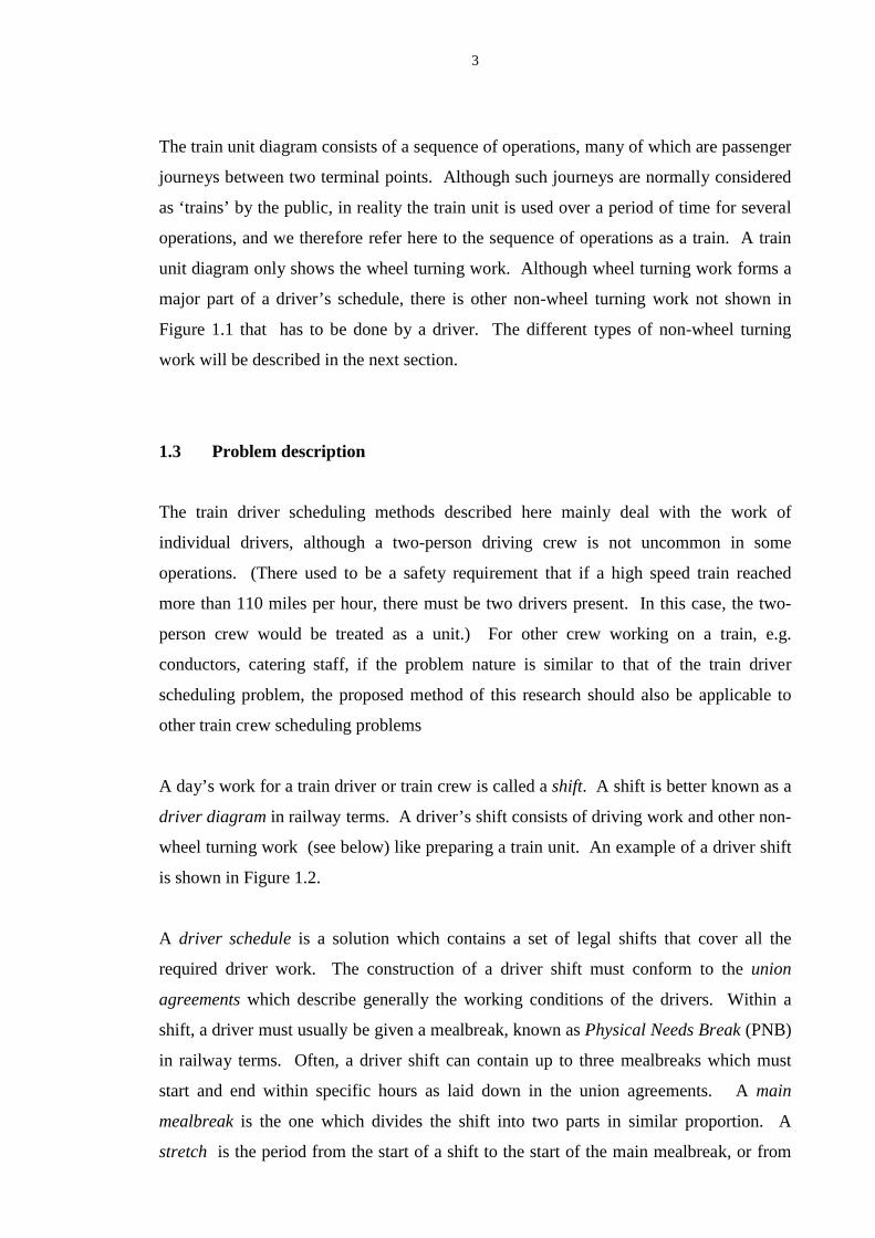
2
This chapter first describes the problem of train driver scheduling and its complexity. It
then compares the train driver scheduling problem with the bus driver scheduling
problem since the latter has some similarities to the train driver problem. The last part
of the chapter discusses the background and the approach used in this research.
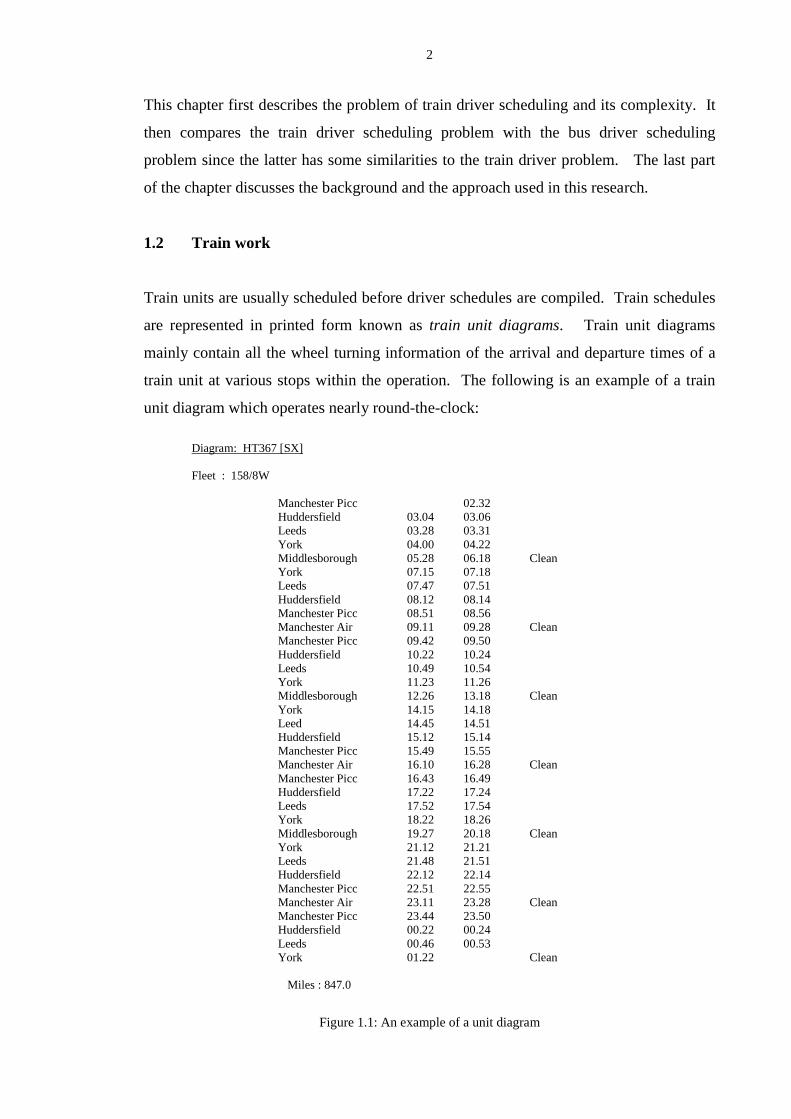
1.2 Train work
Train units are usually scheduled before driver schedules are compiled. Train schedules
are represented in printed form known as train unit diagrams. Train unit diagrams
mainly contain all the wheel turning information of the arrival and departure times of a
train unit at various stops within the operation. The following is an example of a train
unit diagram which operates nearly round-the-clock:
Diagram: HT367 [SX]
Fleet : 158/8W
Manchester Picc 02.32Huddersfield 03.04 03.06Leeds 03.28 03.31York 04.00 04.22Middlesborough 05.28 06.18 CleanYork 07.15 07.18Leeds 07.47 07.51Huddersfield 08.12 08.14Manchester Picc 08.51 08.56Manchester Air 09.11 09.28 CleanManchester Picc 09.42 09.50Huddersfield 10.22 10.24Leeds 10.49 10.54York 11.23 11.26Middlesborough 12.26 13.18 CleanYork 14.15 14.18Leed 14.45 14.51Huddersfield 15.12 15.14Manchester Picc 15.49 15.55Manchester Air 16.10 16.28 CleanManchester Picc 16.43 16.49Huddersfield 17.22 17.24Leeds 17.52 17.54York 18.22 18.26Middlesborough 19.27 20.18 CleanYork 21.12 21.21Leeds 21.48 21.51Huddersfield 22.12 22.14Manchester Picc 22.51 22.55Manchester Air 23.11 23.28 CleanManchester Picc 23.44 23.50Huddersfield 00.22 00.24Leeds 00.46 00.53York 01.22 Clean
Miles : 847.0
Figure 1.1: An example of a unit diagram
3
The train unit diagram consists of a sequence of operations, many of which are passenger
journeys between two terminal points. Although such journeys are normally considered
as ‘trains’ by the public, in reality the train unit is used over a period of time for several
operations, and we therefore refer here to the sequence of operations as a train. A train
unit diagram only shows the wheel turning work. Although wheel turning work forms a
major part of a driver’s schedule, there is other non-wheel turning work not shown in
Figure 1.1 that has to be done by a driver. The different types of non-wheel turning
work will be described in the next section.
1.3 Problem description
The train driver scheduling methods described here mainly deal with the work of
individual drivers, although a two-person driving crew is not uncommon in some
operations. (There used to be a safety requirement that if a high speed train reached
more than 110 miles per hour, there must be two drivers present. In this case, the two-
person crew would be treated as a unit.) For other crew working on a train, e.g.
conductors, catering staff, if the problem nature is similar to that of the train driver
scheduling problem, the proposed method of this research should also be applicable to
other train crew scheduling problems
A day’s work for a train driver or train crew is called a shift. A shift is better known as a
driver diagram in railway terms. A driver’s shift consists of driving work and other non-
wheel turning work (see below) like preparing a train unit. An example of a driver shift
is shown in Figure 1.2.
A driver schedule is a solution which contains a set of legal shifts that cover all the
required driver work. The construction of a driver shift must conform to the union
agreements which describe generally the working conditions of the drivers. Within a
shift, a driver must usually be given a mealbreak, known as Physical Needs Break (PNB)
in railway terms. Often, a driver shift can contain up to three mealbreaks which must
start and end within specific hours as laid down in the union agreements. A main
mealbreak is the one which divides the shift into two parts in similar proportion. A
stretch is the period from the start of a shift to the start of the main mealbreak, or from
4
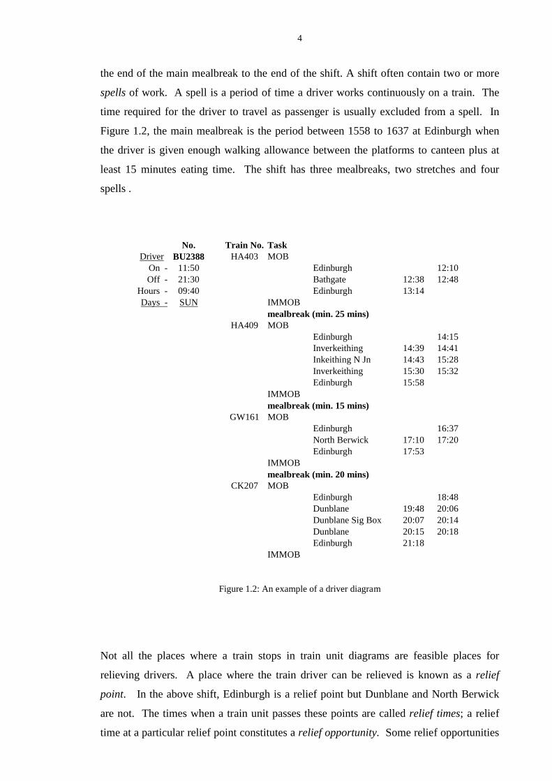
the end of the main mealbreak to the end of the shift. A shift often contain two or more
spells of work. A spell is a period of time a driver works continuously on a train. The
time required for the driver to travel as passenger is usually excluded from a spell. In
Figure 1.2, the main mealbreak is the period between 1558 to 1637 at Edinburgh when
the driver is given enough walking allowance between the platforms to canteen plus at
least 15 minutes eating time. The shift has three mealbreaks, two stretches and four
spells .
No. Train No. TaskDriver BU2388 HA403 MOB
On - 11:50 Edinburgh 12:10Off - 21:30 Bathgate 12:38 12:48
Hours - 09:40 Edinburgh 13:14Days - SUN IMMOB
mealbreak (min. 25 mins)HA409 MOB
Edinburgh 14:15Inverkeithing 14:39 14:41Inkeithing N Jn 14:43 15:28Inverkeithing 15:30 15:32Edinburgh 15:58
IMMOBmealbreak (min. 15 mins)
GW161 MOBEdinburgh 16:37North Berwick 17:10 17:20Edinburgh 17:53
IMMOBmealbreak (min. 20 mins)
CK207 MOBEdinburgh 18:48Dunblane 19:48 20:06Dunblane Sig Box 20:07 20:14Dunblane 20:15 20:18Edinburgh 21:18
IMMOB
Figure 1.2: An example of a driver diagram
Not all the places where a train stops in train unit diagrams are feasible places for
relieving drivers. A place where the train driver can be relieved is known as a relief
point. In the above shift, Edinburgh is a relief point but Dunblane and North Berwick
are not. The times when a train unit passes these points are called relief times; a relief
time at a particular relief point constitutes a relief opportunity. Some relief opportunities

5
are not shown in the driver shifts. For example, train CK207 in Figure 1.2 passes
through Stirling at 1937 and 2026, and relief opportunities exist then. The shift shown
does not use these opportunities, but they might be used in other possible solutions.
When a relief opportunity is chosen for driver relief, one driver will leave the train, to
take a mealbreak, finish their shift or join another train, and another driver can take over
the operation of the train having just started their shift or having finished a mealbreak.
Usually, when a train arrives at a point, there is a time gap before it departs. This creates
a complication as there are two relief times at one location. The arrival and departure
times may or may not be close together. In this case, the relief opportunity contains two
different relief times. A driver can effectively relieve another driver at any time which
falls within the time gap, and this leads to a window of relief opportunities.
1.3.1 Non-wheel turning work
An engine must be started and warmed up at the train depot or elsewhere before the
driver can move it, and the task is known as ‘unit preparation’. Similarly, a train must
be shut down and checked properly at the train depot for the night and the process is
called ‘unit disposal’. At other times when a train unit is temporarily left stationed at a
platform, the train unit has to be turned off first and then later started up again before it is
due to leave the platform. These tasks, known as ‘immobilisation’ and ‘mobilisation’ ,
are usually very short pieces of work. If a unit has been immobilised, a driver has to
‘mobilise’ it before he/she can drive it.
Preparation, disposal, mobilisation and immobilisation form some of the tasks that a train
driver must perform in the course of their duty, and each takes a specific amount of time.
These tasks are also known as ‘soft tasks’ or ‘floating tasks’ because they are not
scheduled to be done at a specific time. In practice, some operators may prefer to
prepare several train units in sequence early in the morning before they are due to start
service. The time required for each of these tasks depends on the type of engine unit.
For example, an HST (High Speed Train) requires 45 minutes for preparation, 20
minutes for disposal, 10 minutes for mobilisation and 5 minutes for immobilisation
whereas a Class 158 (Diesel Multiple Unit) requires 20, 5, 10 and 5 minutes for the
separate tasks respectively. Unfortunately, these types of work are not shown in the unit
diagrams, so they must be identified and marked accordingly in the unit diagrams. Some

6
train work is timetabled for the night, e.g. shunting, preparing trains for early departures.
Hence it is a common feature that a train is in operation round the clock or even in
excess of 24 hours.
1.3.2 Train graphs
For train driver scheduling purposes, it is necessary to gather a set of train diagrams
showing the driving work to be covered. A set of relief opportunities can be identified in
the train diagrams. (There are cases when a train passes a relief point which is not
shown in the train diagrams, in this case, the scheduler must insert such relief
opportunities in the train diagrams.) Any non-wheel turning work like ‘preparation’ or
‘ immobilisation’ can also be marked in the train diagrams.
Throughout this research, the vehicle work for each individual train unit is referred to as
a train graph which can be represented in a graphical format showing all the wheel
turning and non-wheel turning work. The following train graph shows the work of a
train, vehicle 38, in a day from start to end:
Vehicle 38 :
0600 0615 0732 0843 1017 1145 1150 1540 1550 1718 1920 2031 2144 2301 2316
+--+----+----+-----+-----+-+ ..........+--+-----+-------+----+----+-----+---+
G G A A B C C C C C A A D G G
Figure 1.3: A train graph
The horizontal line ‘---- ‘ represents the times that the vehicle needs a driver and each ‘+’
represents a relief opportunity which contains a time and a location point. The dotted line
‘....’ between 1150 and 1540 shows that the train is stationed at a platform and a driver is
usually not required to cover this period. The work between two consecutive relief
opportunities is called a piece of work. Here, the first and the last piece of work, 0600 –
0615, 2301 – 2316 are in fact unit preparation and unit disposal; the pieces of work 1145
– 1150, 1540 – 1550 are immobilisation and mobilisation respectively.
Preparation Immobilisation Mobilisation Disposal

7
1.3.3 Forming a train driver schedule
A shift consists of a number of pieces of work usually drawn from one or more vehicles.
The set of relief opportunities with the associated times and points form the basic
information for driver scheduling. In addition, information on route and traction is also
required. In between two relief opportunities, the section of route the train unit travels is
given a route identifier. Train units in operation can have one of several different engine
units which are known as traction types and a traction type is therefore specific to the
whole train. This information is highly relevant because in train operation, there are
restrictions on the drivers belonging to a particular depot relating to which portion of
routes and which types of traction they can work on.
Train driver scheduling involves distributing the whole train graph into a set of
driver shifts such that:
• every piece of work is assigned to a shift ;
• the shifts which are assigned to a particular depot must conform with the depot’s
route and traction restriction;
• the shifts must also conform to a set of agreed rules laid down in the union
agreement;
• the total number of shifts required is minimised such that individual depot constraints
on the number of shifts are satisfied;
• the total paid cost is minimised.
The construction of a set of shifts satisfying all the constraints and covering all the train
work makes train driver scheduling a difficult and highly constrained combinatorial
problem.
8
1.4 Features of the train driver scheduling problem
The types of operations in train services vary from one extreme which is mainly rural to
the other extreme like the very intensive commuter services. Generally, there are four
main types of service: inter-city, provincial, commuting and rural. The numbers and
distributions of potential points for changing drivers vary greatly, e.g. there are big
differences between commuting and inter-city train services. Commuting train services
in cities have the characteristic of having many and frequent potential opportunities for
changing drivers. Rural and some long distance inter-city services have the opposite
characteristic of having few and infrequent potential points. For very intensive
commuter services, the train driver scheduling problem has a lot of similarities with the
bus driver scheduling problem. Features that exist in the bus driver scheduling problem
can also be found in the train situation but the converse is not always true.
1.4.1 Route and traction knowledge
Route and traction knowledge are major constraints in compiling rail driver schedules,
which do not normally apply to buses. For route knowledge, train drivers may only be
assigned to operate on routes of which they have knowledge. Also they have to maintain
that knowledge by being assigned frequently to work every route within their operating
domain. For this reason, drivers are generally restricted to certain sections of the total
operating area dependent on their home depots. These sections usually overlap, so that it
is not possible to subdivide the problem into areas of specific knowledge. For traction
knowledge, the situation is similar where drivers of some depots may have the operating
knowledge of some power units, if not all of the traction types.
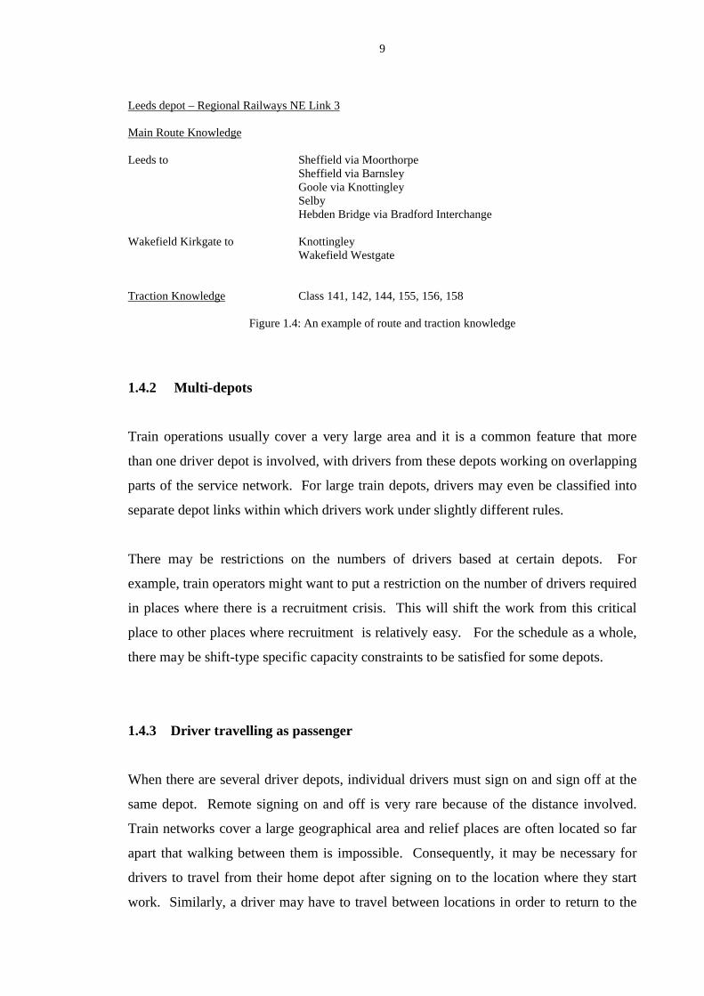
The following is an example of route and traction knowledge referring to a particular
group of drivers within a depot group:
9
Leeds depot – Regional Railways NE Link 3
Main Route Knowledge
Leeds to Sheffield via MoorthorpeSheffield via BarnsleyGoole via KnottingleySelbyHebden Bridge via Bradford Interchange
Wakefield Kirkgate to KnottingleyWakefield Westgate
Traction Knowledge Class 141, 142, 144, 155, 156, 158
Figure 1.4: An example of route and traction knowledge
1.4.2 Multi-depots
Train operations usually cover a very large area and it is a common feature that more
than one driver depot is involved, with drivers from these depots working on overlapping
parts of the service network. For large train depots, drivers may even be classified into
separate depot links within which drivers work under slightly different rules.
There may be restrictions on the numbers of drivers based at certain depots. For
example, train operators might want to put a restriction on the number of drivers required
in places where there is a recruitment crisis. This will shift the work from this critical
place to other places where recruitment is relatively easy. For the schedule as a whole,
there may be shift-type specific capacity constraints to be satisfied for some depots.
1.4.3 Driver t ravelling as passenger
When there are several driver depots, individual drivers must sign on and sign off at the
same depot. Remote signing on and off is very rare because of the distance involved.
Train networks cover a large geographical area and relief places are often located so far
apart that walking between them is impossible. Consequently, it may be necessary for
drivers to travel from their home depot after signing on to the location where they start
work. Similarly, a driver may have to travel between locations in order to return to the

10
home depot to sign off; or to resume duty after a mealbreak; or after a short break to
relieve another colleague.
The following shift shows the level of passenger travel required by a particular driver:
Shift PL09 - Plymouth
DriverOn - 05.40 PAO Plymouth 05.55Off - 12.40 Par 06.50Hrs - 07.00Days - SX MOB Par 07.15
Plymouth 08.15 08.18Newton Abbot 09.00
RELD by PL123
Mealbreak 09.05 - 09.35
PAO Newton Abbot 09.41Plymouth 10.23
Work to be arranged with Supervisor
PAO – passenger travel; MOB – mobilising unit; RELD – to be relieved
Figure 1.5: Example of passenger travel within a shift
The above shift shows that the driver travels as passenger from home depot Plymouth to
Par to start work. At Par he/she mobilises a train and takes it to Newton Abbot. After a
mealbreak, the driver travels as passenger from Newton Abbot back to the home depot to
work as directed by his/her supervisor and then signs off. The above is an example taken
from a manual schedule and it seems a rather inefficient shift as the driver does very
little driving work.
In order to transport drivers between locations and to optimise overall efficiency, drivers
may travel on the trains which are the subject of the current schedule, or on trains run by
other operators. But at times when train service is infrequent, drivers may have to travel
by other forms of transportation, of which the most common types are by taxis or
underground. When this is practically impossible, lodging might be used whereby a
driver would rest for a specified number of hours.
11
1.4.4 Shifts containing work on many different units
As already described in section 1.3.1., there are many types of auxiliary work associated
with the actual wheel-turning work that a driver does in rail operations. These tasks,
together with other non-revenue earning work such as shunting or re-platforming, are
very short pieces of work and fragmented. For optimal efficiency, a schedule may
contain shifts with short pieces of work on many different train units and hence this gives
rise to an enormous number of combinations.
In the bus situation, bus work is less fragmented and does not contain many short pieces.
As a result, bus driver schedules rarely contain shifts with work on more than three
different buses.
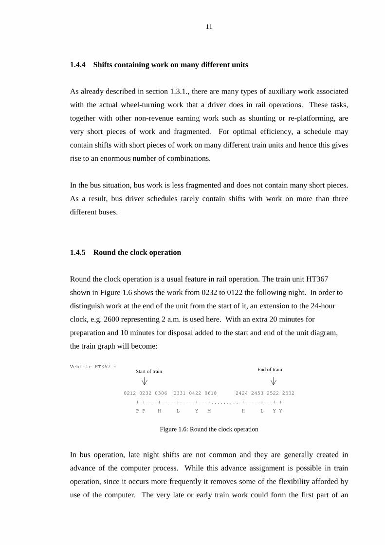
1.4.5 Round the clock operation
Round the clock operation is a usual feature in rail operation. The train unit HT367
shown in Figure 1.6 shows the work from 0232 to 0122 the following night. In order to
distinguish work at the end of the unit from the start of it, an extension to the 24-hour
clock, e.g. 2600 representing 2 a.m. is used here. With an extra 20 minutes for
preparation and 10 minutes for disposal added to the start and end of the unit diagram,
the train graph will become:
Vehicle HT367 :
0212 0232 0306 0331 0422 0618 2424 2453 2522 2532
+-+----+-----+-----+---+ .........-+-----+---+-+
P P H L Y M H L Y Y
Figure 1.6: Round the clock operation
In bus operation, late night shifts are not common and they are generally created in
advance of the computer process. While this advance assignment is possible in train
operation, since it occurs more frequently it removes some of the flexibility afforded by
use of the computer. The very late or early train work could form the first part of an
Start of train End of train

12
early shift or the last part of a night shift from the previous day depending on how it best
contributes to overall efficiency.
1.4.6 Windows of relief opportunities
It is usual that a train is stationed for a period of time at a platform. This gives rise to the
problem of a ‘window of relief opportunities’, i.e. the time of relief being any time
between the arrival and departure of a unit at a relief point which may or may not involve
disposal/preparation allowances. In almost all automatic computer scheduling packages,
shifts are constructed in isolation, so that the selection of one relief time rather than
another is made without considering the whole duty set, provided that the shift is valid.
If every possible discrete minute is used as a separate relief opportunity, the problem size
will increase enormously.
1.5 Union agreements
Although there are many train operating companies, their union agreements are quite
similar in many ways. This may be attributed to the fact that there was only one big
organisation prior to privatisation. The following is a list of conditions which are
commonly used by different operators:
• There may be one, two or three mealbreaks in a shift. There are complicated rules
governing when the mealbreak should occur and how long it should be. The time
range when a mealbreak can occur and its length usually depend on the length of a
shift, e.g. a thirty minutes mealbreak must occur between the third and fifth hour
relative to the start of the shift if its length is less than eight hours; a different set of
rules applies if the length of shift is more than eight hours. These mealbreak rules
sometimes become so restrictive in terms of optimising the schedule that the
scheduler may have to manipulate the starting or finishing times of a shift in order to
ensure that the mealbreak falls into the desirable time range.
• There are restrictions on the length of night shifts whose sign on times are between
midnight and the early hours of the morning which are usually known as ‘unsocial
13
hours’. Sometimes, there may even be a ban on shifts that sign on within these
unsocial hours.
• Length of shifts is usually limited. The shift length is usually no more than twelve
hours maximum.
• Shifts are paid throughout, i.e. from sign-on to sign-off including all the travelling
incurred; allowances for travelling to and from the canteens and the lengths of
mealbreaks.
• There is a restriction on the length of ‘continuous driving’. Continuous driving time
is the time when a driver drives a train unit until he or she is relieved by another
driver. The time always excludes any non-wheel turning work such as unit
preparation and disposal. There are times when a train arrives at a platform in one
direction. The driver then walks from one end to the other end of the train and drives
it away in the opposite direction when the train is due to leave. The time incurred is
called ‘turn round time’ and the driver may be able to take a short break. A driver
may work on a train which has several turn rounds. Diff erent operating companies
may define ‘continuous driving’ according to different length of turn round time.
Usually, any turn round of 10 minutes or less is disregarded and the driving is
considered as ‘continuous’. The maximum continuous driving without a stop is
never longer than those with a stop.
• Similarly, there is a restriction on the total continuous driving time in a shift and the
total is called aggregate driving time.
• There used to be rules governing how many ‘long’ shifts there were in the schedule.
‘Long’ shifts usually refer to shifts whose length is longer than a certain duration.
The most common constraint concerns the proportions of shifts of different lengths.
For example, one constraint was that in a driver schedule, not more than half of the
shifts should have a length greater than eight hours and not more than 20% should
exceed eight hours 30 minutes. Nowadays, with the operating companies trying to
increase efficiency in schedules, these restrictions on shifts of different lengths are
becoming obsolete.
14
• For some companies which operate on long distance services, there are rules
restricting the total mileage that a driver drives in a shift.
1.6 Bus driver scheduling problems – a special case of train driver scheduling
Bus driver scheduling relates more closely to train driver scheduling than any other types
of crew scheduling problems. Both problems are concerned with the allocation of work
to shifts which are very similar in structure, both have similar hours of work with at least
one mealbreak. Both have similar rules in their union agreements. In comparison, all
the features that are in bus operation can be found in the train operation but not vice
versa. Hence, the bus driver scheduling problem can be considered as a special case of
train driver scheduling.
1.6.1 Solving the bus driver scheduling problems using IMPACS
Research into solving the bus driver scheduling problems started at Leeds in the late
1960’s and resulted in the fi rst bus driver scheduling system, TRACS (Techniques for
Running Automatic Crew Scheduling) which was based on heuristics to build up and
then improve a bus driver schedule [1]. A review of TRACS is in Section 2.3.1.1.
Unfortunately, it was not sufficiently flexible for adaptation to wide variations in
circumstances. TRACS was replaced by IMPACS [2, 3, 4, 5] in the early 1980’s. The
first IMPACS system was installed for London Transport Buses in 1984, and is still in
use by their successors. IMPACS consists of a suite of programs performing separate
functions. The system will be described in detail in Chapter Two.
1.6.2 Differences between train driver scheduling and bus driver scheduling
problems
Attempts were made to apply the IMPACS model directly to train driver scheduling with
limited success (Section 1.6.2). The main reason is that there are very significant
differences in conditions between the bus and rail situations. Compared to bus driver
15
scheduling, rail driver scheduling is a far more complex problem. The following is a list
of the differences between them:
• Bus drivers are usually restricted to vehicles from their home depots, so that where
several depots are involved there are effectively a number of separate scheduling
problems. Hence most of the bus driver scheduling problems can be modelled as a
single-depot problem, which is not as complicated as multi-depot ones.
• Although bus drivers do travel on buses as passengers from one place to another
place, the distance travelled is usually small and services are frequent, so that a
constant allowance for the travelling is usually very adequate for scheduling purposes.
Unlike the train situation, there is no need to find out the exact departure and arrival
time for a driver to travel from one place to another place.
• Bus driver shifts usually contain work on no more than three different buses. In fact,
most shifts involve work on two vehicles. This is because bus work is less
fragmented compared to train work and there is no equivalent of the types of non-
wheel turning work like unit preparation and disposal in bus situation.
• There is no equivalent of route and traction knowledge restriction present in bus
driver scheduling problems.
• Mealbreak rules in the bus situation are less complicated than in the train situation,
and the maximum number of mealbreaks very rarely exceeds two.
• Windows of relief opportunities in the bus situation are usually much shorter and
they do not occur as often as in the train situation.
1.7 Background of research
The author is one of the team members of the interdisciplinary research Group,
Scheduling and Constraint Management (SACM) which has evolved out of the
Operational Research Unit at the University of Leeds. Our first insight into the
complexity of scheduling train drivers was gained from a project during 1990-91 in
16
collaboration with the Operational Research Unit of British Rail. It was this project that
laid the foundation of this research.
Before privatisation in the early 90s, the driver scheduling process within British Rail
(BR) was mainly a manual process which was highly dependent on the experience and
skills of the schedulers. There was some computer software (e.g. there was a system
called DIADs) available to assist the manual compilation process. The software mainly
served as a tool to validate drivers’ shifts once they have been created and to print the
schedules in standard ‘driver diagram’ format. The software used had virtually no
optimisation capability in terms of creating complete driver schedules.
When privatisation was imminent, BR started to restructure their operations to look for
higher efficiency in terms of human resources. In order to achieve high productivity,
they needed to find out what could be achieved if the work practices for the drivers were
changed in different ways.
During the summer of 1990 BR commissioned the SACM Group a six-month project to
develop a software tool for accurately estimating the consequences of possible changes
to their current driver scheduling strategy and to determine whether desirable schedules
could be produced under these proposed changes.
The SACM group quickly produced a model which would allow BR to assess the effects
of as many of the proposed operational changes as possible. The model was based on the
IMPACS system developed in the early 1980’s. Since the IMPACS model was
originally based on bus operation, modifications had to be made quickly in order to cope
with the rail operations. The new model provided a good estimate of the numbers of
drivers needed under different work conditions. It was validated by an exercise to
produce the full schedules for a very small operation and to compare the schedules with
the estimates. However, the model was incapable of producing operable driver
schedules in general. This project successfull y helped BR in an exercise to appraise
alternative working practices and to predict the costs of schedules under different
working conditions. Parker et al [6] gives a detailed account of the work carried out in
this project.
17
British Rail was then privatised forming, among others, twenty-five individual passenger
train operating companies for providing train services in Britain. The work practices
under the newly privatised companies underwent changes from a very rigid mode to a
more flexible mode in which better and more efficient schedules could be produced.
Under private ownership, the operating companies started to restructure their operations
and there was a need for a much higher degree of automation in schedule production.
In the course of the 1990-91 project the SACM group gained a good knowledge of the
requirements for a scheduling system for British Rail[7]. However, with rail
privatisation looming, the uncertain future of British Rail prevented it from financing
the research and development of such a system. Funding was therefore sought from the
EPSRC, who funded a two-year project on research into the scheduling of rail driver
shifts. This was followed by another three-year grant from the EPSRC to develop
generic methods for public transport driver scheduling with the aim to produce a more
robust methodology for both bus and rail industries.
1.8 Research approach
At the conclusion of the 1990-91 project, it followed that any system developed for
scheduling British train drivers must either be developed from scratch or must be adapted
from systems designed for other transport modes, of which bus was by far the closest to
rail operation. Although there were substantial differences between the bus mode and
the train mode which made it impossible to use a bus-related system directly for rail
operation, it was still possible for IMPACS to produce reasonably realistic rail schedules
in some simplified test cases during the 1990-91 work. This gave us the confidence that
an approach similar to that used in IMPACS could be used for the rail situation.
One important consideration in choosing a method for solving train driver scheduling
problems is that the method should be flexible enough, and should not be affected by
changes in the scheduling conditions. One main reason for flexibilit y is the drastic
change in the structure of the rail industry. Before rail privatisation, there was one big
organisation overseeing all the operations through a traditional vertical management.
There was generally one common set of rules and practices for driver scheduling. After
privatisation, although most individual operating companies still retain this legacy of

18
work practices, there is a demand for individual companies to change the work practices
gradually in order to improve productivity and to compete with other train operating
companies. After privatisation, some of the scheduling rules become more flexible than
before whereas new rules are being introduced into the union agreements from time to
time. The complexity of the problem is therefore remain more or less the same as
before. Hence a scheduling method that is flexible enough to cope with various
scheduling conditions is essential.
One main factor in deciding whether the IMPACS model should be adopted is its two-
stage approach which is flexible enough to cater for different working conditions. The
first stage of the method is called the GENERATION stage which builds a large set of
feasible shifts and is the only process which might be affected by different working
conditions. The second stage which is called the SELECTION stage is relatively domain
independent. The following diagram summarises the approach used by IMPACS :
Stage one: Stage two:
GENERATION SELECTI ON
Figure 1.7: IMPACS framework
The GENERATION stage forms a large set of feasible shifts and the SELECTION stage
uses a mathematical programming method using a set covering formulation to select
from a large set of possible candidate shifts a subset to form a final schedule. Changes in
the working conditions or other external factors will only affect the type of shifts to be
input to the selection process and hence the mathematical part will not be affected.
Build a large set offeasible shifts
Solve a setcovering problemwith LP
Branch and Boundto find integersolution
19
Hence, in this research it is considered worthwhile to follow the set covering model and
the mathematical technique used in IMPACS. The GENERATION in IMPACS system,
however, is based on bus operation and cannot be adapted for train driver scheduling
because of the complexity of the rail problem. An entirely different method is needed in
the shifts formation stage so that valid and operable shifts can be produced. When the
method is developed, the mathematical process in SELECTION can be used as a tool for
producing schedules. However, the size of the rail problems sometimes makes the
SELECTION process less robust in terms of yielding a final schedule than the bus
situation.
Following the above framework, the areas of research in each stage are identified and
prioritised.
1.8.1 GENERATION
The first priority is to devise methods in GENERATION which create legal shifts for the
SELECTION stage. This priority is often overlooked by researchers because of the
practical and applied nature of research. It is important to have legal shifts because the
ultimate goal of solving the train driver scheduling problem is to produce results which
are operable.
The paramount objective of the shift creation process is to ensure that all the generated
shifts must be legal, i.e. satisfaction of all constraints and rules. In order to produce legal
shifts, the process must possess much problem specific knowledge in train driver
scheduling. This can be achieved by using heuristics in order to express such
knowledge. Using heuristics would also make it easier to incorporate domain specific
constraints and rules incrementally. The research required here is identification of
conditions and requirements in which the train driver scheduling domain differs from bus
driver scheduling. New or enhanced heuristics will be developed to meet the
requirements.
Once the components in the GENERATION stage had been tested vigorously and most
of the domain specific requirements are correctly interpreted and catered for, the next
20
step of this research is to enhance system performance and robustness in the
SELECTION stage.
1.8.2 SELECTI ON
The second priority is to improve the computational efficiency of the SELECTION
process. This involves identifying and improving upon a specific component of the
scheduling process that is computationally intensive.
The SELECTION process used by IMPACS is an ILP algorithm [2] solving the set
covering problem and allowing users to specify simple side constraints. As described in
Figure 1.7, the ILP method in IMPACS involves two components. First it solves the set
covering problem as an LP by relaxing the integer requirement and finds an optimal
solution with a total number of shifts which is often non-integer. This is called a relaxed
solution. Then a target is set using the sum of the shift variables involved (rounded-up if
it is non-integer). A branch and bound process will follow which aims to solve a zero-
one ILP model.
The ILP process has over the years been shown to be successful in producing quality
schedules. However, owing to the nature of branch and bound, sometimes it might fail
to produce an integer solution. This usually happens when the process automatically
stops the tree search because a stipulated number of nodes have been explored and the
search tree is getting too large to handle practically. Some failures can be attributed to
problems becoming bigger and more complex to solve than before. There are three
things that need to be improved:
• ability to guarantee yielding an optimal or near optimal integer solution
• speed - even with today’s computing power, the LP and then the Branch and Bound
process can be time consuming
• size of problems – like all standard ILP process, there is a limit in the size of the
problem it can handle
21
In recent years, two completed Ph.D. theses have been directed at the method used to
find the relaxed solution [8, 9]. Their work will be described in Chapter Seven. Their
work has significantly enhanced the speed and the capability of the LP process. Fores’s
work also enhanced the capability of the process so that a much larger set of candidate
shifts can be input to the LP. However, little work has been done on improving or
replacing the branch and bound process, which can be time consuming and difficult.
In this research, it is considered worthwhile to attempt to improve the robustness of the
SELECTION process in terms of yielding a final solution by investigating possible
methods to replace the branch and bound process. Since the SELECTION process is not
specific to the problem domain, the use of metaheuristics (e.g. genetic algorithms, tabu
search) as an alternative to produce the final solution through the exploration of the
search space seems attractive. One reason is that there has been a large community of
research in metaheuristics in recent years and this will benefit the current investigation.
Amongst different metaheuristics, Genetic Algorithms (GAs) are chosen to be used to
further our investigation. GAs simulate natural evolution by developing populations of
solutions to a problem and allowing new solutions to be formed by mating processes and
mutations. These have a particular advantage that the concept is not only interesting but
also easily understood and they are more acceptable to the end-users than other
metaheuristics. Also, there has been an enormous amount of research into GAs. Other
members of our group have been doing research into GAs on bus driver scheduling
problems and the results of their research are encouraging [86, 91]. Details of the
research by other members of our group are in Section 8.4. In this research, the use of
Genetic Algorithms to replace the branch and bound component in the ILP process will
be investigated, tried and critically assessed.
In summary, this research has the following tasks :
1. The first and the most important task is to develop solution strategies and a generic
method for train driver scheduling meeting all the major operational constraints and
requirements for rail operation in the U.K. This should be an evolving process
because the method is to be applied to different sets of real life data from a number of
train operating companies and is then refined in the light of test results. It should,
therefore, incrementally enrich the capability of the method to cope with more
complex issues.

22
2. The second task is to attempt to tackle some of the computational diffi culties and to
explore the use of GA’s as an alternative to the mathematical approach.
1.9 Benefits of scheduling train drivers by computer
One significant cost for a train operating company, apart from the rolling stock, is that of
its drivers. It is therefore essential to keep these costs to a minimum. A scheduling
system that can produce operable schedules and save even a small proportion of these
would clearly be very useful. There are also other benefits that an automatic train driver
scheduling system can provide, for example, it can help the management to assess the
likely impact on costs should some of the working conditions change.
The scheduled train service is revised and published every six months and hence driver
schedules are also revised half-yearly. Although most of the changes are usuall y small,
schedulers still have to make some adjustment to the driver schedules to ensure that the
changes are incorporated into the driver schedules. This makes the compilation of
schedules a very tight process. (Individual operators, before they can finalise their
operating schedules, must submit their schedules or ‘bids’ to RailTrack for evaluation.
After evaluation, RailTrack, who may revise the schedules, pass the schedules back to
the operators as an ‘offer’ and the operators may accept or re-bid to Railtrack in the
subsequent cycle.) In addition to the usual planned summer or winter timetable that
may be required, there may be changes in timetabled service, or planned and unplanned
engineering works for a specific set of days. These will also result in revision of the
driver schedules.
The compilation of schedules is usually done by specialist ex-BR staff, who (once
trained in the skill) often remained within that position, and the driver schedules they
produce are usually very efficient. There are many tedious arithmetic checks to be done
to ensure that shifts are valid and conform to the route and traction restrictions and union
agreements. As a result, the usual practice is to rely heavily on precedent. The use of
computers in train driver scheduling can assist the scheduler in many ways. Good
computer software for train driver scheduling can produce good schedules much more
quickly than manual processes. This factor is becoming more important, since train
23
operating companies are coming under increasing pressure for a variety of reasons to
revise services more frequently (e.g. pressure from the Office of Rail Regulator).
Service revisions cannot be put into operation until the corresponding train and train
crew schedules have been compiled, and in order to get the maximum benefit from the
changes, it is essential that the schedules should be as efficient as possible. This puts a
heavy workload on the schedulers, and a computer system which can produce a good
schedule quickly can be very helpful.
From the management point of view, a computer driver scheduling system can be used
as a planning tool that can help to assess the effect on driver schedules if there is a
change in operation. For example, it can be used to predict the distribution of work
amongst depots, as well as to construct potential new schedules under a range of
different working conditions. Once basic data is established, it is very easy to adjust the
data to cater for different scenarios. This can help the management to evaluate the costs
of alternative operating scenarios by producing full schedules as a guarantee for a range
of strategies; e.g :
• to consider a depot closure or to create a depot, canteen, or a relief point
• to alter route and traction knowledge
• to change working conditions for higher productivity
• to move drivers’ work between depots for whatever reason, e.g. to cope with
recruitment problems
• to effect changes in different types of allowances, e.g. signing on, signing off,
walking
In today’s computer technology, computer scheduling systems are no longer expensive
to set up. Most personal computers have the processing power and storage capability
which far exceed many mainframe computers in the 1980’s. However, there have so far
been very few implementations of train driver scheduling systems in this country. This
is partly because the problem is difficult to solve and partly because some schedulers
have the suspicion that computer scheduling systems pose a threat to their job security

24
and therefore feel reluctant to use them. On the issue of job security, a computer
scheduling system needs skilful and experienced schedulers who are familiar with how
schedules are constructed to get the best use out of it. They are the ones with the
expertise and knowledge to rectify the problem when the answer the system produced is
not what they expected. This research concentrates on tackling this complex problem
and creates a system that can be used by experienced schedulers who know the effects of
changing system parameters.
25
Chapter Two
Literatur e review
2.1 Introduction
An exhaustive literature search has revealed very little practical driver scheduling work
for the U.K. train industry in the academia. Although some train companies in the U.K.
and in some European countries are known to be using some computerised driver
scheduling systems (Sections 2.2.3, 2.2.4), there are few publications on these systems.
However, the bus driver scheduling (or urban transit driver scheduling) problem, which
shares some similarities with the train problem, was first tackled in the early 1960's and
the subject has been well researched since then. There have been seven International
Workshops on computer-aided scheduling of public transport [10, 11, 12, 13, 14, 15, 16].
This chapter will concentrate on the review of a range of solution methods in both train
driver and bus driver scheduling as evidenced by published papers. Publications on train
driver (or crew) scheduling will be reviewed first and then followed by a review on the
well-researched bus driver scheduling problems. Lastly, the problem of air crew
rostering will be reviewed briefl y.
26
2.2 Computerised train driver scheduling systems
2.2.1 British Rail
Among the earliest publications in train driver scheduling, Ellis and Savin [17]
described the computer scheduling systems developed by British Rail. Their systems are
based on interactive techniques. There are three types of schedules involved: long
distance, local services and ancillary work. For long distance schedules, users use a set
of scheduling commands to specify certain relief points. The system will then retrieve
the timetables of trains between these points and derive a solution using an assignment
technique. For the ancillary work schedules, owing to its small size compared with the
others, a conventional batch processing approach is used. The ancillary work pieces or
‘mini-items’ are matched with the spare capacity on the driver’s schedule where this is
possible. If necessary, extra drivers are scheduled to work on the mini-items only. The
local service schedule is the most complex in which the trains work much shorter
distances within a small area. The local service schedules involve a core area and a
periphery. The core area contains all the crew depots and relief points whereas the
periphery contains no crew relief point except that meal breaks may be taken in the
periphery if facilities are available. The system for scheduling local services uses colour
graphics to represent trains on a VDU. Shifts are built up one at a time and are checked
by the system, and the work covered is removed from the display.
An attempt had been made to use mathematical programming methods by British Rail
for the train driver scheduling problem, but this approach was later abandoned. By the
time when British Rail was privatised in the early 1990’s, there was still no known
automatic driver scheduling system being used by British Rail.
2.2.2 The New Jersey Railway System
Tykulsker et al [18] describe a train driver scheduling system developed for the New
Jersey Railway System in the early 1980’s. The objective of developing such a system is
to enable the management to analyse quickly the implication of work rule changes on
27
labour costs for union negotiations. The type of service involved is mainly commuter
train type with a typical two peaks situation. There is no mention of the size of the
problem or the number of crew depots involved. However, the requirement that shifts
must start and end at the same location suggests that there could be more than one crew
depot. The nature of the problem is very similar to that of a bus driver scheduling
problem except that there are some additional features which are specific to train
problems. For instance, crews occasionally perform ‘deadheading’ trips (passenger
travelling) while travelling on service trains. Similar to route knowledge restriction,
crew members can only be assigned to a single line or group of lines according to the
crew’s depots. Passenger travel is dealt with by means of overlapping. Overlapping is
the situation when a train is covered more than once in the solution, only one shift will
be in service and the others will travel as passengers at the same time. This gives the
driver few alternatives for passenger travelling because the driver will be restricted to
travel on trains which only run on the group of routes to which the driver can be
assigned. The drawback of using overlapping for passenger travelling will be discussed
in Chapter Four.
The problem is solved in three steps. Crew shifts are first generated. Next the shifts are
costed and the last step is to determine the schedule by solving a set covering problem
using a mathematical programming method. Tykulsker et al adopt a special structure
suggested by Ryan and Foster [19] in the shift generation stage. Ryan and Foster argue
that by linking a given train to its first available connection in building up an assignment,
the relaxed LP solution is often integer and therefore branch and bound search will not
be needed.
Tykulsker et al report that the relaxed LP solution often has a high percentage of
overlapping. In some occasions, there may be loops in the solution for the drivers to
travel as passenger and these are called ‘deadheading’ loops. A deadheading loop refers
to the situation when a particular shift is assigned to a set of consecutive trains so that
each train on the loop is also covered by another shift (or shifts) and the departure point
of the first train and the arrival point of the last train on the same loop are the same. In
such cases, the loop is eliminated from that particular shift to form a new shift provided
it is still valid.
28
If the relaxed LP solution is non-integer and all the deadhead loops are removed, a new
integer set covering problem is solved using the incumbent solution plus the new
loopless shifts. Tykulsker found that the solutions to the new relaxed problems were
either integer, or very nearly integer. Even if branch and bound is employed, the value
of the objective function is very close to that of the non-integer objective function.
The fact that there is a high percentage of deadhead loops suggests that the shift
generation process seems to be very restrictive and very few alternatives are available for
the mathematical programming stage.
2.2.3 The Italian State Railways
Caprara et al [20] is one of the most recent publications on train crew scheduling.
Caprara et al give an account of the development of a new crew planning system for the
Italian State Railways. The Italian State Railways operates a vast network with a crew
workforce of about 25,000 drivers and 15,000 conductors located in about 50 depots.
The system described is a planning system for locomotive scheduling (not mentioned in
the publication), crew scheduling and rostering. For crew scheduling, Caprara et al use
a traditional approach which involves two phases based on a set covering model. The
first phase is to generate a very large number of feasible shifts while the second phase
selects the best subset of all the generated shifts so as to cover all the 'trips' at minimum
cost.
The shift generation phase sequences a number of ‘trips’ to form a shift which must start
and end at the same depot. A ‘trip ’ is defined as segments of train journey which must
be serviced by the same crew without rest. However, it is not mentioned whether there
are any more relief opportunities on each trip. It is likely that a trip may simply be the
train journey between two major crew relief points without any intermediate relief points
allowed. This would then greatly reduce the size of the problem instance. Caprara et al
describe how the trips are sequenced into a shift according to some sequencing rules, one
of which is that a crew can only change between trains at the same location. This
implies that drivers travelling between two different places is not allowed. This will
restrict the number of shifts being formed to a great extent.
29
When drivers are required to passenger travel between places after signing on and before
signing off, this will be shown up as overlapping in the solution. As has already been
discussed above, this way of resolving passenger travel is too simplistic because the crew
will be restricted to travel on the same train that the crew’s shift has been assigned to.
There is no mention of any route or traction restriction in the problem. It is likely that
these restrictions have been ignored in order to simplify the problem further.
Caprara et al use a set covering model for the shift selection phase. The approach used is
based on a Lagrangian relaxation method and the information provided by the
Lagrangian cost cj(u) is used for finding the solution. The approach consists of three
main steps. The first step finds a near-optimal Largrangian multiplier vector. The
second step uses the information provided from the vector and ranks the shifts of the
incumbent best solution. The final step is to select a subset of shifts with a high
probability of being in an optimal solution. The three-step procedure is iterated. After
each application of the three-step procedure, a ‘refining procedure’ is used to improve
the solution. The paper does not mention how the ‘refining procedure’ works.
The results are based on problem instances with up to 5000 trips (rows) and just over a
million of shifts variables (columns) and the number of shifts in the schedule is just over
one thousand. The simplifications on the problem would have prevented some crucial
shifts from being generated. It is likely that the shifts generated are very restrictive in
order to reduce the possible number of combinations and as a result the schedules
produced would not be very near the optimum if some of the crucial shifts are missing.
In most of the train driver scheduling problems in the U.K, the simplifications on the
shifts generation phase may be unacceptable because they result in shifts that are
inoperable.
2.2.4 The Dutch Railways
Morgado et al [21] describe the CREW_NS system developed for the Dutch Railways
for the scheduling of drivers and guards. The CREW_NS is developed by the
Portuguese company SYSCOG and is based on an earlier scheduling system, CREWS,
which was originally developed for the Portuguese Railways. Dutch Railways have
about 5000 train drivers and guards. The features of the driver scheduling problem
30
described in the paper include some major features found in the British train driver
scheduling problems, for instance, passenger travel, route and traction knowledge.
CREWS can be used in one of three modes: (i) the manual mode in which the system
provides no active support; (ii) the semi-automatic mode in which the system gives
suggestions to the scheduler on the appropriate next steps in the planning process; (iii)
the automatic mode in which the system tries to create a schedule automatically.
Personnel ‘tasks’ are fi rst generated according to rules that specify the number of
personnel resources required for each type of activity. A ‘task’ is the association of an
activity with the personnel resources. The tasks are sequenced according to some criteria
and are distributed among partitions (sub-division of the problem). The scheduling
process creates a schedule by grouping in sequence the tasks of the sub-problem into
shifts according to the labour agreement rules.
The algorithm of building up a schedule automatically is based on a modified version of
Beam Search (Bisiani [22]). Beam search is an AI search technique which is based on
heuristic rules to discard non-promising alternatives in order to keep the size of the
alternatives as small as possible. The method for constructing a schedule is to build a
large search tree starting from an initial state when tasks are ready to be scheduled, to a
goal state when all the tasks have been scheduled. Each node represents a partially built
shift or the start of a new shift and each arc represents a heuristic operator to generate all
the possible alternatives. Heuristics are used in order to eliminate unpromising
alternatives. A schedule is formed by finding a path through the tree while at the same
time minimising the cost of the schedule. The algorithm, to some extent, tries to mimic
the planning methods used by the scheduler and it has some similarity to those used in
the TRACS system (see Section 2.3.1.1). However, there are not enough details in the
publication for a comparison with the TRACS system.
The paper does not report any direct comparison on the quality of the schedules
produced by the system with that produced by any other techniques or with any manual
schedules. The system is dependent on rather crude heuristics for constructing the
schedule. Since the scheduling rules and constraints are embedded into the scheduling
process, the system might be difficult to adapt to new scheduling conditions. Also,
implementing different what-if situations may be difficult if these what-if situations
31
require changes to the heuristics. It is doubtful if this heuristic based technique would
yield a near optimal solution.
2.3 Bus crew scheduling systems
Compared to train driver scheduling, bus driver scheduling is a well-researched area.
There are many papers detailing the approaches and their applications. The most
important findings are compiled in the seven volumes of papers on Computer-aided
Scheduling of Public Transport edited by Bodin and Bergman[10], Wren[11],
Rousseau[12], Daduna and Wren[13], Desrochers and Rousseau[14], Daduna et al[15]
and Wilson[16].
The most widely used computerised crew scheduling systems in the public transport
sector are probably: IMPACS (called CREWPLAN in BUSMAN) [3, 4], HOT II from
Germany [23, 24, 25], and HASTUS[26, 27, 28, 29, 30, 31] from Canada. There are
other systems known to be used in the public transport sector such as Teleride-Sage,
UMA and Austrics. Details on Teleride, UMA and Austrics have not been published and
so they will be omitted from this review.
The approaches reported for the bus crew scheduling problem can be roughly divided
into two groups:
• A heuristic approach which includes constructive and improvement techniques or a
mixture of heuristics and other algorithms such as the matching algorithm or the
assignment algorithm. Some of the matching or assignment approaches may involve
the use of a mathematical programming formulation (for example, the HASTUS
system);
• A mathematical Programming approach which formulates the problem as a set
covering or set partitioning model which is solved by using mathematical
programming methods

32
The classifications are not distinctive because, as Willers[8] comments, it is usual to find
that some Mathematical Programming approaches may involve heuristic techniques to
some extent or vice versa.
2.3.1 Heuristic Approaches
This section reviews systems that use heuristic approaches for solving bus driver
scheduling problems. In recent years, the use of metaheuristics is becoming popular.
Metaheuristics are modern heuristic techniques that use a more general approach [32]
than the traditional problem specific heuristics for solving large combinatorial
optimisation problems. Examples of metaheuristics being used for driver scheduling
problems include Tabu Search, Simulated Annealing and Genetic Algorithms. Since the
use of Genetic Algorithms will be discussed in Chapter Eight and a review of using
Genetic Algorithm in driver scheduling problems will be presented there, a review of
that method is omitted from this section.
2.3.1.1 The TRACS System
Research into bus driver scheduling at the University of Leeds started in 1967 and
originally employed a number of different heuristics as experience developed. This
work was consolidated into the TRACS (Techniques for Running Automatic Crew
Scheduling) system in the 1970’s.
The system first constructs a schedule whose shifts satisfy all the constraints, leaving
some stretches of work uncovered if necessary. Then the process will refine the schedule
by reducing the number of such stretches, and at the same time, improve the quality of
the final schedule. Parker and Smith [1] give a detailed account of the system.
TRACS uses a list of parameters together with some special routines written for the
specific scheduling conditions of individual bus companies. The heuristics used for
building the initial solution are sophisticated and aim to produce a good initial solution.
This is because the refinement heuristics were unlikely to perform well with a poor
initial solution. The shifts TRACS produced can have two or three spells. The

33
construction of the initial solution starts by forming early shifts. This is achieved by first
marking the latest time by which the first driver of each early bus must be relieved for a
mealbreak. At each stage the bus with the earliest remaining marked time will be
considered for forming a new shift. Some pieces of early shifts are deliberately left
unallocated to provide for the creation of split shifts (shift with a long mealbreak) later.
Late and middle shifts are constructed similarly, except that the heuristics work
backward from the end of the day. Split shifts are then formed by pairing up the
unallocated work pieces. After that, any unallocated work is attached to existing shifts if
possible, otherwise, extra shifts are formed to accommodate the uncovered pieces.
The refinement heuristics contain two sets of routines. One set attempts to reduce the
number of shifts. Each shift is analysed to determine whether the work in it can be
accommodated in other shifts. The routine redistributes work between shifts so that
shifts having long spreadovers are allocated more work. This will make short shifts
shorter so that they might be eventually absorbed into other shifts. Another set of
routines is for cost reduction. There are several routines to achieve this. One routine is
to break up the shifts into two halves and then re-combine them by solving an
assignment problem. Other routines involve swapping work pieces between shifts and
switching changeovers of a shift to another relief time so that a reduction in cost can be
achieved.
The system produced good results for several bus companies usually after two or three
months of research to adapt the initial heuristics to new conditions. The main
disadvantage of the system is that it always takes a considerable time, usually several
months, to adapt the heuristics to new requirements.
2.3.1.2 The COMPACS System
COMPACS (COMPuter Assisted Crew Scheduling) was developed in the early 1980’s
(Wren et al [33]). It was later incorporated into the BUSMAN scheduling package (see
Wren and Chamberlain [34]). COMPACS is an interactive system combining the
heuristics of TRACS and the interactive features of an early interactive system known as
TRICS (Techniques for Running Interactive Crew Schedules). TRICS was developed by
the Operational Research Unit at the University of Leeds in the late 1970's.
34
COMPACS can be used as an interactive tool for the scheduler to construct the entire
schedule himself/herself, and each duty constructed is validated by the system. One
useful feature is that it can give an estimate on the likely number of shifts of each type.
The estimate can be useful because it guides the scheduler as he/she builds up the
schedule interactively. COMPACS can also produce an entire schedule automatically by
means of a simplified version of the heuristics of TRACS for constructing the initial
solution. However, the refinement heuristics of TRACS are not incorporated into the
system and hence the quality of the schedule produced may be poor.
2.3.1.3 The RUCUS-II System
RUCUS-II (RUn CUtting and Scheduling)[35, 36] is a bus and crew scheduling system
which originated from the RUCUS systems [37] in the 1970’s. The system was
developed by the Urban Mass Transportation Administration and was installed in several
bus companies.
The original RUCUS system used refinement techniques similar to those of TRACS, but
a much cruder initial heuristic; it was moderately successful because many American bus
operators had much slacker scheduling rules than were prevalent in the UK. Work on
the original RUCUS system was reported at the Chicago Workshop in 1975 [10].
The system uses heuristics to form one-piece shifts in which the driver stays on the same
bus throughout without a mealbreak. Then two-piece early and late shifts are formed in
stages. Finally, any unallocated work pieces are added to the schedule as ‘trippers’, i.e.
over-time pieces. After an initial schedule is formed, some improvement algorithms are
used to improve the schedule. Since ‘trippers’ are expensive and undesirable, the
algorithm tries to eliminate them by incorporating them into any two-piece shifts. The
algorithms also reduce the costs of the schedule. There are two ways to do this: first, by
possibly swapping work pieces between pairs of shifts; second, by switching the relief
times which are the end of a piece of one shift and at the start of a piece of another shift
to the previous or subsequent relief time.
35
Later, RUCUS was substantially revised [35] and was reported in the Montreal
Workshop in 1983. The heuristics for forming the initial solution and for subsequent
refinement are very similar to those used by its predecessor. The main differences
between the two systems are that the parameters specification of the new system is
simpler and these can be modified as the schedule is being formed; and the running of
the process is interactive rather than in batch mode. This gives the users more control
over the formation of the schedule. The RUCUS-II system only forms shifts with up to
two spells. This will limi t the system’s ability in getting good solutions since, in many
of the problem instances, shifts with more than two pieces are often crucial in forming
the near optimal solution.
Ball et al [36] propose enhancement heuristics to the RUCUS-II heuristic based on the
switching and shifting algorithms. The switching algorithm involves swapping the work
pieces using a graph-matching algorithm which minimises the cost. The shifting
algorithm involves taking one vehicle graph at a time and finding the best relief
opportunities on that graph by solving an assignment problem. The relief opportunities
on the other vehicle graphs remained unchanged during this process. Then the same
procedure subsequently applies to all vehicle graphs. Ball et al report that good results
are achieved using the enhancement algorithms.
The RUCUS-II system was installed in many organisations, apparently successfull y,
probably owing to the slackness of the constraints. However, it proves very
cumbersome, and has now probably been completely abandoned.
2.3.1.4 The HASTUS System
Work on the HASTUS system started in the 1970's and was reported in several of the
International Workshops [26, 27, 28, 29, 30, 31]. The HASTUS system is believed to be
the most widely used public transport scheduling system in the world today. The system
was originally developed by the University of Montreal and later jointly with Giro Inc.,
Canada. After many years of development and having the backing of many North
American organisations, the software is very sophisticated and user-fri endly and
provides a lot of facilities and different versions in several languages. There are three
36
installations in the U.K.: Lothian Regional Transport, Busways (Tyne and Wear) and
First Main Line (South Yorkshire).
The crew scheduling part of HASTUS contains two components, HASTUS-macro and
HASTUS-micro. A new driver scheduling method called Crew-Opt [38, 39, 40] with a
column generation approach has been developed since the late 1980's and will be
described in Section 2.3.2.2.
The crew scheduling part of HASTUS first cuts the bus work into spells or stretches of
work. The approach used is to relax the crew scheduling problem first and then solve the
relaxed problem by using a mathematical model. Users first define periods between 15
and 60 minutes, and relief opportunities are approximated to occur only at the beginning
of a period. All feasible shifts with two or three spells of work are generated. A linear
programme (LP) then selects a set of shifts with minimum cost that will provide the
number of drivers required in each period. HASTUS-macro provides an estimate of the
likely number of shifts required and hence it can also be used as a planning tool. The
next step involves cutting the actual bus work as closely as possible according to the
information provided by the relaxed solution. The process cuts the bus work into work
pieces by solving a shortest path problem. A matching algorithm is then used to generate
shifts from the work pieces [41] and a schedule is formed. Several heuristics are used to
improve the solution.
HASTUS has been originally developed for the North American market where
constraints are usually quite slack. However, it may not work as well when the
constraints are very tight, as in most UK situations. That may explain why there are
relatively few U.K. installations.
37
2.3.1.5The HOT II System
HOT (Hamburger Optimierungs Technik) [24] was developed and has been used by the
schedulers at the Hamburger Hochbahn AG (HHA) since the 1970's. Völker and
Schütze [25] gave an account of the recent developments of HOT II at the Sixth
Workshop in 1993. HOT II consists of five modules: basic data management, sensitivity
analysis, vehicle scheduling, duty scheduling and duty rostering. Here, only their driver
scheduling algorithm is described.
HOT II employs a multi-stage process. The work of each bus is scanned to determine
possible driver relief opportunities that could be included in an early shift. Bus work is
split into pieces at these relief opportunities. The pieces are sorted by starting time and
form a list which will be used for forming shifts. Each piece will be considered in
chronological order. Valid shifts are formed by linking this particular piece with other
pieces in the list and are given a weight which is a combination of the cost and the
quality of the shift. The shift with the lowest weight is chosen. Based on the shift just
chosen, a mealbreak chain is formed by building further shifts containing the work
before the pick-up time (end of mealbreak). After the first shift is formed as above, other
shifts are formed starting with the next available early piece, until all pieces up to a pre-
determined time have been allocated. The remaining early shifts are formed in a similar
way except that in any iteration all pieces which are suitable and not yet assigned are
considered as possible starting pieces of a shift, and the best shift out of all these is
chosen. This will allow the computer a wide choice although the process is rather time
consuming. Some starting pieces may not be used and will be picked up later when split
shifts are formed. Late shifts are formed backwards from the end of the day using a
mirror image of the above process.
The unused pieces are now grouped into vehicle blocks and each block is processed from
the beginning and cut into pieces of maximum length for half shifts. The half shifts are
then combined using a variant of the Hungarian algorithm. Split shifts are formed in a
similar way except that any short pieces are linked in pairs if possible to form longer half
shifts. So some of the split shifts may ultimately contain work on up to four buses.
After that, any uncovered pieces will be accepted as unscheduled pieces.
38
In recent years, there is no new publication on the research and development of the HOT
II system.
2.3.1.6The BDS System
Carraresi et al [42] use a network flow approach to solve the bus driver scheduling
problem. Their system, BDS, described by them in the paper published in 1988, is
installed at ATAF, the public transit company of Florence. The system includes an
algorithm for solving network models and a user interface built around the query
language, SQL. Feasible pieces of work are represented as nodes, and the arc connecting
two nodes is part of a shift. A single piece of work is represented as a self-loop. A
schedule is derived from finding a subset of arcs such that each node is falling upon
exactly one arc in the subset.
The process first cuts the vehicle work into work pieces by solving a minimum cost
network flow model. The is based on a Lagrangean relaxation approach, which yields a
lower bound and a feasible solution which indicates how the vehicle work is to be
partitioned. The next phase consists of three steps: first, work pieces are matched by
solving a maximum cardinality minimum cost matching problem; then any remaining
unmatched pieces are combined to form three spell shifts; lastly, all the remaining
unmatched work pieces are matched to form new but longer single piece work. The last
step may be executed again if the last step results in new pieces being formed.
The BDS system was tested on a very large problem and produced a schedule with 809
shifts. The users can then interactively change the solution in order to satisfy particular
union constraints not included in the mathematical model. The fact that users have to be
involved in the scheduling process may perhaps undermine the quality of the solution
produced by the automatic process.
2.3.1.7 A Lagrangean relaxation based heuristic
The approach used by Ball and Benoit-Thompson [43] (also published in 1988) in
solving the bus driver scheduling problem bears some similarities with the approach used
39
by Carraresi et al [42] as described above. Ball and Benoit-Thompson modelled the
problem into a shortest path problem solved by a matching algorithm. This approach is
validated on sample problems from the Washington Metropolitan Area Transit Authority
(WMATA).
A graph is formed for each block where each node represents a relief point or the garage
and a possible piece of work is represented by an arc. The vehicle work is partitioned by
solving a shortest path problem. They used a Lagrangean relaxation approach to solve
the network flow model. The solutions produced achieved a reduction in pay hours and
are comparatively better than those created by the system used by WMATA.
2.3.1.8 The MICROBUS System
The MICROBUS system is a planning and schedule tool and covers all the planning
steps from the drafting of timetable to the production of rosters for the drivers. An
account of the system is given by Bertram et al [44] in their 1988 published paper.
The crew scheduling part uses heuristics to construct an initial schedule. The process
first forms shifts according to different categories of vehicle blocks. Some vehicle routes
are short and therefore unsuitable for single shifts. First a vehicle block is cut into one,
two or three shifts exactly without a mealbreak. Then the remaining vehicle work is cut
into one or two shifts and any remaining uncovered piece is allowed. The shifts formed
up to this stage still have no mealbreak. Any unallocated work pieces are to be absorbed
by extending the work pieces of the already formed shifts as far as possible. Then shifts
with mealbreaks are formed to cover any uncovered pieces.
The subsequent improvement routine uses an assignment algorithm. The aim is to
minimise the total ‘unproductive periods’ in the schedule just created. ‘Unproductive
periods’ are the time when breaks are required. There were no results reported and
hence it is difficult to evaluate the crew scheduling method used. However, the method
would be unsuitable where mealbreaks are compulsory, as in most U.K. situations.
40
2.3.1.9The Ravenna System
The system, described by Martello and Toth [45] , was developed for a bus company in
the Italian town of Ravenna in the 1980’s. The crew scheduling problem is complicated
by the fact that there exist three peak periods within a day, a midday peak during lunch
time, the morning and the evening peaks. Every driver whose shift covers the midday
peak has to have a mealbreak immediately before or after the peak. The method of
forming a schedule follows the traditional way: it determines an initial crew schedule and
then uses improvement techniques to improve it. The initial schedule is constructed in
two steps. The first step constructs shifts covering the midday peak period and the other
step determines shifts for the rest of the day.
Since each vehicle which spans the lunch peak has to be covered by at least two drivers,
the strategy used here is to reduce the number of drivers by using three drivers to cover
two vehicles’ work over the lunch peak. The routine therefore identifies pairs of such
lunchtime buses that can be assigned to three drivers. The algorithm for forming shifts
for the rest of the day uses a greedy heuristic. There is no description of the
improvement techniques used in the system.
As the system is specially tailored for the Ravenna’s midday peak situation, it is highly
unlikely that it is applicable to other problems.
2.3.1.10 A Tabu Search approach
A recent publication by Cavique et al [46] describes the use of heuristics combined with
Tabu Search. The approach used here contains two stages. The fi rst stage uses a
constructive heuristic similar to TRACS to provide an initial feasible solution that cover
all the ‘trips’ in the problem. A ‘trip ’ is a piece of work on a vehicle such that the relief
points concerned must be the terminus points. This is followed by two alternative
improvement algorithms to reduce the number of shifts in the initial solution based on
Tabu Search. Tabu Search is a metaheuristic which has an iterative search procedure
whereby the algorithm moves from one solution to another in a defined neighbourhood
under certain deterministic conditions in order to avoid being trapped in local optima.
Tabu Search relies on the use of flexible memory structures which ‘ remember’ recent
41
moves and put them on a Tabu list. Glover [47, 48, 49, 103] gives a comprehensive
introduction on Tabu Search.
One of the two improvement routines iteratively removes some inefficient shifts as well
as their adjacent shifts from the current solution and then re-constructs new shifts so that
all the pieces are covered. The algorithm uses an evaluation function to make sure that
‘difficult trips’ will be combined with others at an early stage of the algorithm, avoiding
inefficient shifts. The algorithm is very efficient in improving the initial solution after a
few iterations but then takes a significant amount of time to find a better solution.
The other improvement routine seems to be quite complicated. The algorithm first
divides the vehicle work into blocks of feasible work pieces. Then it uses a matching
graph algorithm to form a schedule. The schedule contains shifts with a maximum of
two pieces and some shifts may have only one piece of work. The process contains three
elementary operations: ‘shift operation’ which shifts the relief time of a work piece to
another relief time; ‘cut operation’ which cuts one piece into two pieces; ‘merge
operation’ which merges two pieces into a single piece. For each block divided as
above, one of the above operations is selected randomly. A revised matching graph is
then formed and the ‘moves’ involved are ‘ tabued’ for a number of iterations. The
process stops after it reaches the maximum number of iterations without any
improvement. At each iteration, a feasible solution will be obtained and stored.
Cavique et al evaluated the above refinement algorithms using data provided by Lisbon
Underground and comparisons were made between the results obtained by the algorithm
and the manual procedures. The results represent a reduction of up to 3.6% on the
manual solutions. However, Lisbon Underground considers that any schedule with an
average of 4.5 driving hours per duty is of very good quality. This suggests that the
initial manual solutions may not be very efficient. The problem could have been
simplified because all the relief opportunities are at the start or the end of a trip (i.e. the
termini), and never happen during the trip. Another unusual feature is that all shifts have
an identical cost. Also, the lack of three and four spell shifts in the solution method may
indicate that the solution could still be further improved had three or four spell shifts
been allowed. Like other heuristic methods, the approach presented here may not be
easily adaptable to a different company using a different set of rules.

42
2.3.1.11 Overview of the heuristic approach
In the early years when automatic bus crew scheduling systems were being developed,
heuristic systems had had their successes. Systems which are specifically designed for a
particular company can be full y tailored to suit the company’s need and these systems
tend to produce satisfactory results, e.g. the TRACS system [1], the HOT system [24, 25]
and the RUCUS system [10, 35, 36, 37].
One major problem with a heuristic system is that the heuristics themselves had to be
adapted to deal with new situations, and that such adaptation might take a considerable
time, usually over several person-months of research. Another problem is that the
heuristics developed for these systems are often based on the skill and expertise of the
schedulers. Although the system can work much faster than humans, the quality of the
schedule produced may not be significantly better than the manual schedule. This is
because heuristics build a schedule by constructing shifts one by one, unless the system
has the ability to backtrack, the shifts built at a later stage may have very few
combinations to choose from. Although these heuristic systems usually have a
refinement routine similar to a local search to improve the initial solution, the ways most
refinement heuristics work indicate that the best schedule they achieve would likely be a
local optimum. Cavique et al [46] used the Tabu Search technique to escape from local
optima. However, the techniques they used are complicated and the problem may have
to be simplified to a certain extent.
Another popular approach is the ‘cut and match’ method. Each vehicle work is cut into
work pieces and a schedule is formed by matching these work pieces, resulting in shifts.
Some of the methods reviewed formulate the problem as a network flow model which is
solved as a shortest path problem. However, most of the systems which use the ‘cut and
match’ approach would result in leaving some work pieces uncovered. These uncovered
work pieces may have to be represented as ‘trippers’ or ‘overtime’ shifts. Another
observation of methods using this approach is that the shifts produced mainly are two-
spell. Although BDS [42] produces three spell shifts, these shifts are formed after the
two spell shifts have been formed and the remaining uncovered pieces are then attached
to these two spell shifts to form three spell shifts. As a result, some efficient three spell
shifts may never be formed.

43
The systems reviewed are specially designed for bus crew scheduling or similar
problems so they are not applicable to the U.K. train driver scheduling problems. In
order to apply any of the above systems to the train problem, substantial changes have to
be made to the heuristics in order to accommodate the many different features of the
train problem.
2.3.2 Mathematical programming approach
The most successful bus driver scheduling systems are based on a mathematical
programming approach. Shepardson [50] gave a concise formulation of the basic
problem. Wren and Rousseau [51] presented a summary of the Mathematical
programming based systems and gave detailed accounts of some of the successful
systems. Briefly, the problem is tackled by first generating a set of all possible legal
shifts and selecting a subset of shifts (solution) which can between them be assigned to
all the work pieces of the problem with the objective that the total cost of the selected
shifts is minimised or the number of shifts is minimised, or both.
The approaches commonly used are either set partitioning in which each piece of work
has to be covered by exactly one shift; or set covering in which any piece of work can be
covered by more than one shift. Since in real life problems, the number of possible legal
shifts can be enormous, there is usually some restriction or relaxation to the full problem
so that the problem can be reduced to a manageable size.
2.3.2.1 The IMPACS System
The IMPACS system provided the author with a starting point for the current research.
It has been briefly introduced in Chapter One. Its mathematical formulation is based on
a set covering model and the ILP process will be discussed in detail in Chapter Seven
and will not be introduced here. Wren and Smith [4] give a full description of the
system. Work on IMPACS started in late 1970’s and by the early 1980’s, a prototype
was successfully demonstrated to London Transport who then commissioned further
development of the system [52]. The project was completed by the end of 1984 and the
IMPACS system was installed in London Transport at the end of 1984. IMPACS was

44
installed for Greater Manchester Buses in 1985. The system was later included into the
BUSMAN scheduling system [34] which has since then been installed for a number of
bus and light rail operators in the U.K. and some overseas countries.
The IMPACS system uses various heuristics to reduce the problem size and contains a
number of routines which are to be run in sequence. The routines are described as
follows:
1. EST estimates whether any potential driver relief opportunity is likely to be critical in
forming a good schedule, and makes a list of such critical opportunities. It also
sensibly decomposes particularly large problems.
2. SELECT examines the total bus work and reduces the number of pieces of work to
be covered by rejecting some of the relief opportunities as unlikely to be necessary to
the formation of a good schedule.
3. GEN generates a large set of possible shifts satisfying all the legal requirements in
the union agreements. This process will be described in Chapter Five.
4. COMPARE and EVEN are for eliminating any shifts which are considered to be less
crucial towards forming a good schedule compared with the others.
5. ZIP is a mathematical process which fi rst relaxes the integrality constraints and
solves the relaxed LP. Unless the relaxed LP solution is integer, it then looks for an
integer solution using branch and bound. Search stops as soon as a sufficiently good
solution is found. A full discussion of the Integer Linear Programme (ILP) process is
presented in Chapter Seven
6. SPRINT translates the integer solution into a list of shifts and applies heuristic
improvement to the solution and finally prints the schedule
7. OVER is used when a large problem has earlier been decomposed into sub-problems.
It analyses the schedule produced by ZIP and identifies shifts that are less efficient,
for example, shifts that contain overlaps or shifts that have a low work content.
45
Users can then specify the percentage of work and certain types of shifts to be carried
forward to another sub-problem
8. COMBINE is used in decomposed problems to combine the results of all sub-
problems into a workable schedule. After the sub-problems have been combined,
SPRINT is called to improve and print the final schedule
As already mentioned in Chapter One, in 1990, the Operational Research Unit of the
British Railway Board commissioned the Leeds team to provide a system which could
give accurate estimates for evaluating the likely changes to the train driver schedules
under different operating scenarios. Within a short space of time, IMPACS was adapted
slightly to cope with a few of the important train driver scheduling requirements. This
work is described by Parker et al [6]. Owing to the generally large size of the train
problem instances, the amended system has been used to run only up to the relaxed phase
of the LP process which will then give a total of the values of the shift variables as the
estimate. The system has been useful in providing good estimates. In some of the
simpler problems, the estimates are validated by completing the ILP process to obtain an
integer solution.
Since IMPACS was originally designed for the bus driver scheduling problem, it is
difficult to apply the system directly to the complicated train driver scheduling problem.
Also, like most of the mathematical based systems, it has an inherent problem of not
being able to tackle large problem instances, and often train driver scheduling problem
instances are very large. Sometimes the branch and bound search may fail to find any
integer solution.
2.3.2.2 The Crew-Opt method of HASTUS
Crew-Opt was described by Desrochers and Soumis [38, 41] and Desrochers et al [39].
It became part of the HASTUS system and has been used in a number of experiments
and trials for a wide range of problems including a train company (East Japan Railway).
It uses a set-covering method that is based on column generation techniques.
46
The approach used involves several steps. It first generates a set of feasible shifts. A
subset of shifts is then selected and, based on this subset, a linear programming solution
is obtained by relaxing the integrality of the shift variables. After an LP solution is
obtained, more feasible shifts with negative reduced costs are created in order to improve
the current LP solution. The problem of generating new feasible shifts is formulated as a
shortest path problem with constraints. The process of finding the relaxed LP and the
generation of shifts with negative reduced costs is repeated until the LP optimum is
reached. Then the process enters a branch and bound phase which also uses a column
generation method to solve the LP at each node of the branch and bound tree.
Theoretically, this column generation approach could achieve optimal or near optimal
solutions. However, in practice, the process has to generate a large number of shifts and
solve a number of the LP problems at the same time and it will be computationally
expensive. Rousseau and Desrosier [40] reported solving several crew scheduling
problems using Crew-Opt, one of which is the East Japan railway problem. Three of the
problems are solved on a line-by-line basis and the line with the largest problem has 38
shifts. For the East Japan problem, there is no report of whether the typical features of
the train problem are present, for instance, multi-depot, passenger travel, route
knowledge or traction knowledge. However, the drivers may have to ‘lodge’ at the depot
for at least 6 hours and hence a shift may span over two workdays.
The East Japan case consisted of two different problems. One of them involved around
77 shifts and the other had around 160 shifts. The larger problem had to be decomposed
into three subsets. A slightly changed heuristic was used to obtain an integer solution
from the LP solution. At each step of the branch and bound process, one variable was
selected and fixed to a value of 1 before the problem was re-optimised with column
generation. There is no report on the precise computer running time for solving all the
problems. However, the computer time required to solve the large train problems was
reported in the order of 24 hours on a Sun Sparc 10/31 machine.
47
2.3.2.3 The CRU-SCHED System
Mitra and Darby-Dowman [53] describe the crew scheduling system CRU-SCHED
which was tested by the Dublin City Services bus company in the early 1980’s. There is
an earlier crew scheduling system call NUCRU reported by Mitra and Welsh [54].
The approach used by CRU-SCHED involved generating a large set of valid two spell
shifts and then, based on a generalised set partitioning model, using mathematical
programming to select a subset of shifts to form the schedule. In a generalised set
partitioning model, both ‘overcover’ and ‘undercover’ were allowed. Schedulers had to
specify the number of shifts of each type to be used by the system in the schedule. In
addition, an extra constraint which is the limit on the average work times of the shifts of
each type was also specified. The system only created two spell shifts and extension to
three spell shifts was planned but not reported. The system was reported to be used by
the Rome Transport Company (ATAC) [55] for scheduling bus and crew simultaneously.
However, there has been no new publication on the latest system in recent years. The
inability of the system to create shifts with more than two spells means that it will
produce poor schedules if it is applied to train problems.
2.3.2.4 The EXPRESS System
Falkner and Ryan [56] describe a bus crew scheduling system based on a set partitioning
model specially developed for Christchurch Transport, New Zealand. An earlier version
of EXPRESS and a study of the use of set partitioning are presented in [57]. The
approach used is to decompose the problem into three sub-problems, not according to the
size but according to the type of shifts formed. The package for solving the Integer
Linear Programming model is a version of ZIP similar to those being used by IMPACS
and TRACS II . The scheduling conditions in Christchurch seem very similar to those in
the U.K. with two peak periods. Shifts are classified as early, middle, late and split. A
mealbreak has to be included in each shift. Mealbreaks for early shifts occur after the
morning peak whereas mealbreaks for middle and late shifts can occur any time when
appropriate.
48
The system uses the method of ‘Next-Availables’ reported in publications [58, 19]. This
method uses a generalisation of the petal route concept to restrict the total number of
combinations. Ryan and Falkner suggested that if each trip has a unique next-available
(i.e. a unique subsequent trip) then the solution to the set partitioning problem will be
naturally integer. However, this is too restrictive and may result in a poor solution. The
compromised way is to have several next-availables for each piece of work.
EXPRESS consists of three stages:
1. Only middle and late shifts are selected. All bus work finishing too late to be
included in any of the split shifts must be included but there is no need to cover any
earlier bus work. Shifts are then generated, and a minimum number of middle and
late shifts are found by the ILP process. In order to limit the number of shifts,
mealbreak constraints are used to ensure that the number of drivers having meals at
certain times is less than or equal to the maximum number of concurrent meals
allowed. These constraints can be violated in cases when it is not possible both to
use the minimum number of middle and late shifts and to satisfy the mealbreak
constraints. The work covered by the solution is removed from the data.
2. Most of the early shifts are selected in the second stage. All bus work left after stage
one but excluding the bus work which is too late to appear in an early shift is
considered here. All the work that could be part of a split shift is removed. Shifts
are generated and a minimum number of shifts are selected by solving the ILP of the
subproblem. Work covered by the solution is removed from the data.
3. Extra early shifts and the half split shifts are formed in the final stage. A solution is
obtained by solving the ILP of the subproblem. The half shifts are then combined
together to form full split shifts.
Falkner and Ryan acknowledge that the disadvantage of decomposition of the problem
into three separate stages is the loss of interaction among the subproblems. Although
very efficient schedules may be obtained in each subproblem, the sub-division may have
already prevented some good combinations of work between subproblems from being
generated. Another drawback of the approach is that half shifts are formed before they
are combined to form split shifts. In order to ensure that all the half shifts can be linked
49
together to form split shifts, extra side constraints are introduced for this purpose. The
decomposition was based on early, middle, late and split types of shifts and this shift
type classification is not relevant to the train driver scheduling problem. The system is
not applicable to train problems unless substantial changes are made. Also, the system
was tested on small problem instances with fewer than 50 shifts.
2.3.2.5 Overview of the mathematical approach
Compared to systems using heuristic approaches, systems that use a mathematical
approach based on a set partitioning or set covering model seem to be more successful in
producing good schedules. Mathematical programming based systems are relatively
easy to be adapted to different scheduling conditions. This is because the formation of
legal shifts is often not integrated into the mathematical process. If scheduling
conditions are changed, at worst, only the process of shift generation needs to be
changed.
However, using a mathematical approach has its limitations. In many real life problems,
the number of rows may be several thousands and the number of columns may be well
over a million. It may need a great amount of computer time to solve large problem
instances. Also the use of branch and bound for obtaining an integer solution may
involve searching a very large tree and often it is the most time consuming and difficult
part of the whole ILP process. Therefore certain techniques have to be employed to
reduce the problem to a computationally manageable size. This may involve using
decomposition techniques or some heuristics for problem reduction such as eliminating
shifts that are thought to be inefficient. Schedulers usually do not like decomposition as
they perceive it as creating sub-optimal solutions. However, Wren and Smith[4],
suggested using a decomposition strategy which could have minimal effect on the quality
of the solutions.

50
2.4 Review of other approaches in solving driver scheduling problems
In recent years, new approaches have been attempted in different directions in solving
the driver scheduling problem, mostly in the bus problems. The use of Genetic
Algorithms will be reviewed separately in Chapter Eight.
Layfield et al [59] developed a constraint programming based pre-processor which
reduces the number of relief opportunities. The work was primarily developed for the
bus driver scheduling problem. Reducing the number of relief opportunities will
effectively reduce the number of rows, and the problem size is reduced. The approach
used is based on forming good mealbreak chains throughout the morning period.
Layfield et al suggested that if reasonable mealbreak chains are found, potentially useful
relief opportunities will be contained within these chains. The problem is formulated as
a constraint satisfaction problem which is solved by using a constraint programming tool
called ILOG Solver[60].
Variables are based on the relief opportunities. Each relief opportunity is represented by
two variables: one defining the work covered by a shift up to this relief opportunity; one
defining the work covered by a shift after the relief opportunity. The domains of the
variables are subsets of relief opportunities available that can form either the start or the
end of a mealbreak. Legal shifts are dynamically formed during the process so that
efficient mealbreak chains can be ascertained. Although at present, only mealbreak
chains covering the morning period are considered, the process is capable of forming
mealbreak chains for the evening period by simply ‘inverting’ the evening bus work to
resemble morning work.
Curtis et al [61] reported the use of constraint programming for forming bus driver
schedules. They tackle the scheduling problem as a set partitioning problem in which
every piece of work must be covered by exactly one shift. Shifts are first generated by
using TRACS II which will be used as an input set to the constraint programming
process. The constraint programming model is formulated such that pieces of work
become variables and the domain of each variable is the set of indices of the shifts that
cover the piece of work in question. The problem is constrained by the set covering
property where if a piece of work is assigned to a shift, Si, all the other pieces of work
51
covered by that shift will also be assigned to Si. Conversely, if a shift is not used by one
of the pieces of work it covers, it cannot be used by any of the others.
In order to enhance the quality of the solutions produced by the process, Curtis et al
made use of the information provided by the relaxed LP solution as a value and 'variable
ordering' guide. The relaxed LP solution gives the coverage of the pieces of work which
are usually fractional values. Details of how to incorporate the relaxed LP solution into
the process are described in the paper. The formulated problem is solved by using ILOG
Solver’s standard backtracking algorithm. The process was tested on relatively small
problems and the results produced have the same number of shifts as produced by the
ILP process of TRACS II .
Forsyth [62] describes a new approach using a stochastic combinatorial optimisation
method called an Ant System for constructing driver schedules. An Ant System, created
by Dorigo et al [63], is a new Evolutionary Algorithm that has been used in recent years.
The idea of an Ant System comes from studying the behaviour of ants searching for a
food source. Each ant leaves behind a pheromone trail that can be detected by other ants.
When ants look for food, ants move at random and lay down trails of pheromone; the
ants which find the shortest path are likely to return soonest and their trails are therefore
strongest. Subsequent ants are most likely to follow the shortest trail which becomes the
dominant trail. A large set of shifts was first generated and used inside the ant
environment. The environment is defined as a network of nodes connected by links and
the ants traverse the network making choices at each node about which link to follow
next. A trail left by an ant is defined as a solution and its quality is measured by a
combination of the number of shifts, work uncovered and the cost. A pheromone level is
assigned to a trail according to the quality of the solution. The movement of ants within
the environment is probabilistic depending on the pheromone intensities and the
closeness levels in the environment. As the process progresses, pheromones left by an
old trail will fade and eventually disappear unless the trail is visited by more ants. The
system cycles for a specified length of time and eventually a dominant trail will emerge
which represent the best solution. The system is still under development and no results
have been reported.

52
2.5 Air crew rostering or pairing systems
The crew scheduling problems for the airline companies are quite different from train
and bus driver scheduling problems. The ‘crew pairing’ problem is to determine a set of
flight legs that can feasibly be flown by an airline crew. A crew pairing is composed of
one or more legal duties which is a single workday for a crew, separated by rest periods.
A duty is composed of activities such as fli ght legs and ground time whereas a pairing is
a round trip originating and terminating at the same crew home base and varies between
one and up to three weeks for long haul fli ghts. The formation of crew duties is heavily
constrained by the maximum continuous working time and the minimum rest period in
the union agreement. In addition, relief opportunities are few and far between and meals
can be taken whilst the crew are at work. The air crew scheduling problem is to find a
set of pairings which covers flight legs at a minimum cost.
The traditional approach used to solve the air crew scheduling problem is based on a set
partitioning model which is solved by mathematical programming based methods. The
model is further constrained by the crew base restriction such as maximum number of
hours or limited number of crew available. Marsten and Shepardson’s [64] approach is
to find an optimal solution to the relaxed LP and then, using a branch and bound
algorithm, to find an integer solution. The branching strategy used is to decide which set
of variables should be responsible for covering a particular row instead of simply
branching on an individual variable. Hoffman and Padberg [65] used a branch and cut
approach to solve the set partitioning model with home base restrictions. They employed
a constraint generator that cuts off parts of the LP feasible region that do not contain
integer solutions. Ryan [66] used a set of improved linear algebra routines used by the
ILP process of IMPACS and TRACS II to solve very large air crew rostering problems.
Instead of shifts, patterns of work over several days are generated and a feasible schedule
is selected by using the ILP process to solve a set partitioning model. Ryan's system is in
use by Air New Zealand.
For large size problems, more recent methods have used a column generation approach.
Fores [9] gives an account of the various approaches that involves column generation for
air crew scheduling.

53
Owing to the substantial differences between train driver scheduling and air crew
pairings problems, it is unlikely that successful solution methods for air crew pairings
can be transferable to train driver scheduling or vice versa.

54
Chapter Three
The TRACS II driver scheduling system
3.1 Introduction
As already described in Chapter One, the first task of the research started in September,
1994 is to develop solution strategies and a generic method for train driver scheduling
meeting nearly all of the operational constraints and requirement for rail operation in the
U.K. Within a few months of the start of this research, a new method for generating train
driver shifts was developed by the author. The new method coupled with an enhanced
mathematical programming process developed for shift selection at Leeds over many
years led to the development of a system for train driver scheduling. By the end of 1994,
a prototype system was ready for testing. Since then, the capabilities of the system have
been extended throughout this research. Driver schedules were produced on a test basis
for a number of train operating companies, and the developing system was given the
name TRACS II (Techniques for Running Automatic Crew Schedules Mark II ). This
chapter outlines the components of TRACS II ; its input data files and results. Chapters
Four and Five will discuss the new method for generating operable train driver shifts in
detail.
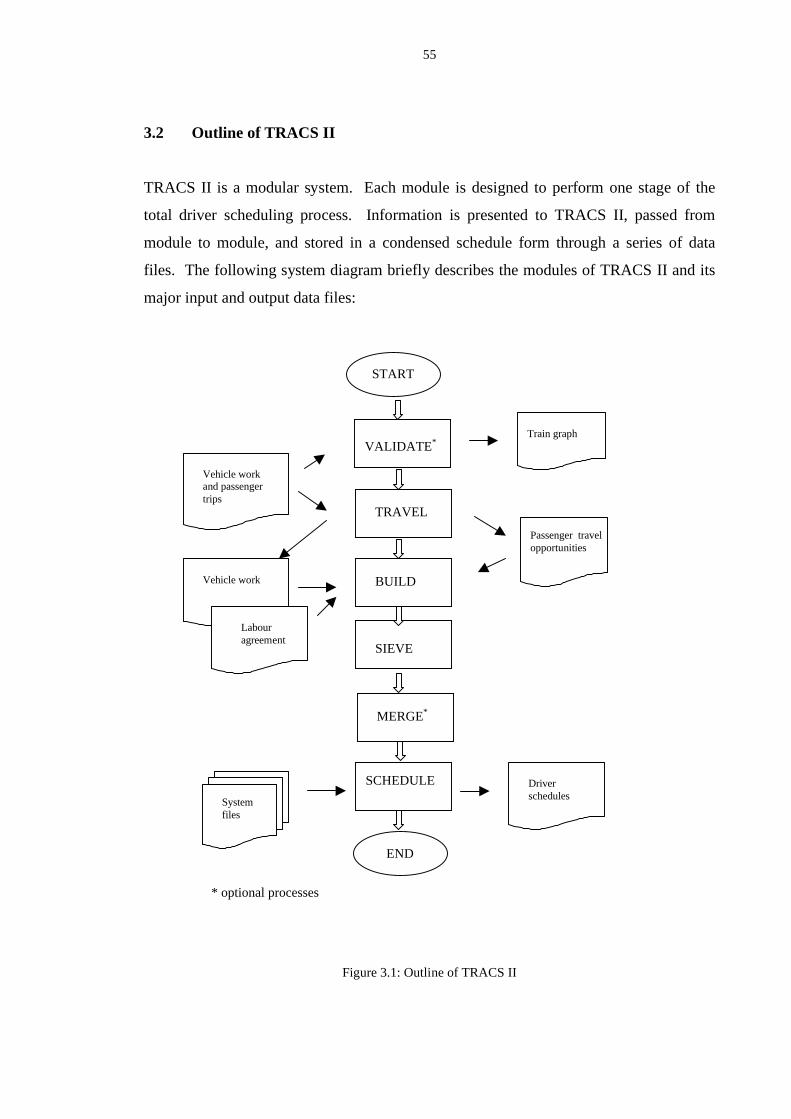
55
3.2 Outline of TRACS II
TRACS II is a modular system. Each module is designed to perform one stage of the
total driver scheduling process. Information is presented to TRACS II , passed from
module to module, and stored in a condensed schedule form through a series of data
files. The following system diagram briefly describes the modules of TRACS II and its
major input and output data files:
Figure 3.1: Outline of TRACS II
TRAVEL
BUILD
SIEVE
START
Vehicle workand passengertrips
Vehicle work
Labouragreement
VALIDATE*
SCHEDULE
Systemfiles
Driverschedules
END
MERGE*
* optional processes
Train graph
Passenger travelopportunities
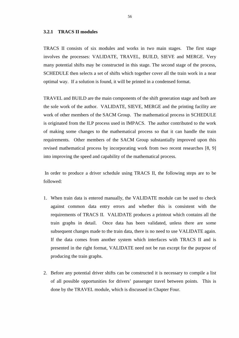
56
3.2.1 TRACS II modules
TRACS II consists of six modules and works in two main stages. The fi rst stage
involves the processes: VALIDATE, TRAVEL, BUILD, SIEVE and MERGE. Very
many potential shifts may be constructed in this stage. The second stage of the process,
SCHEDULE then selects a set of shifts which together cover all the train work in a near
optimal way. If a solution is found, it will be printed in a condensed format.
TRAVEL and BUILD are the main components of the shift generation stage and both are
the sole work of the author. VALIDATE, SIEVE, MERGE and the printing facility are
work of other members of the SACM Group. The mathematical process in SCHEDULE
is originated from the ILP process used in IMPACS. The author contributed to the work
of making some changes to the mathematical process so that it can handle the train
requirements. Other members of the SACM Group substantially improved upon this
revised mathematical process by incorporating work from two recent researches [8, 9]
into improving the speed and capability of the mathematical process.
In order to produce a driver schedule using TRACS II , the following steps are to be
followed:
1. When train data is entered manually, the VALIDATE module can be used to check
against common data entry errors and whether this is consistent with the
requirements of TRACS II . VALIDATE produces a printout which contains all the
train graphs in detail. Once data has been validated, unless there are some
subsequent changes made to the train data, there is no need to use VALIDATE again.
If the data comes from another system which interfaces with TRACS II and is
presented in the right format, VALIDATE need not be run except for the purpose of
producing the train graphs.
2. Before any potential driver shifts can be constructed it is necessary to compile a list
of all possible opportunities for drivers’ passenger travel between points. This is
done by the TRAVEL module, which is discussed in Chapter Four.

57
3. The BUILD module next forms a very large number of potential driver shifts based
on the train data and a set of parameters describing the scheduling rules to be
followed. The method used in BUILD will be discussed in Chapter Five.
4. If the set of potential shifts produced by BUILD is too large, this can be refined by
the SIEVE module until a reasonable number of potential shifts remain for
submission to the following mathematical process. SIEVE incorporates a range of
possible filtering techniques, producing refined lists of potential shifts for input to
MERGE or SCHEDULE. The optional MERGE module is used when potential
shifts have been generated according to more than one set of parameters used by
different BUILD runs. The resulting sets of shifts produced may be merged after the
SIEVE process. SIEVE and MERGE will be discussed briefly in Chapter Five.
5. The remaining potential shifts will be input to SCHEDULE, the mathematical
process which selects from the potential shifts set, a subset of shifts as the final
schedule. SCHEDULE minimises the number of actual shifts used and total cost.
The SCHEDULE process includes the production of a summary schedule file for
printing. If a solution is found, it will be printed. The mathematical process will be
described in Chapter Seven.
3.2.2 Input data files for TRACS II
The system is driven by three main sets of input data. The first set Vehicle work and
passenger trips contains the train work (represented as a set of relief opportunities) to be
covered by drivers and other train trips to be used for drivers to travel as passengers.
The file also lists the relief points to be used, including driver depots, and gives details
of, or pointers to, travelling times between every pair of relief points, signing on and off
allowances for all the depots and the mealbreak details. It is the principal input file of
train work for which drivers are to be provided, and specifies geographic data, such as
when and how drivers can travel between points in the network. All the route and
traction restrictions per depot are also specified here. This file is used by TRAVEL
which determines paths for drivers travelling as passengers. TRAVEL outputs a data fil e
which contains only the vehicle work required for driver scheduling. It also produces a
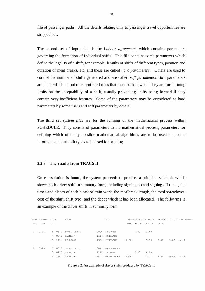
58
file of passenger paths. All the details relating only to passenger travel opportunities are
stripped out.
The second set of input data is the Labour agreement, which contains parameters
governing the formation of individual shifts. This file contains some parameters which
define the legality of a shift, for example, lengths of shifts of different types, position and
duration of meal breaks, etc, and these are called hard parameters. Others are used to
control the number of shifts generated and are called soft parameters. Soft parameters
are those which do not represent hard rules that must be followed. They are for defining
limits on the acceptability of a shift, usually preventing shifts being formed if they
contain very inefficient features. Some of the parameters may be considered as hard
parameters by some users and soft parameters by others.
The third set system files are for the running of the mathematical process within
SCHEDULE. They consist of parameters to the mathematical process; parameters for
defining which of many possible mathematical algorithms are to be used and some
information about shift types to be used for printing.
3.2.3 The results from TRACS II
Once a solution is found, the system proceeds to produce a printable schedule which
shows each driver shift in summary form, including signing on and signing off times, the
times and places of each block of train work, the mealbreak length, the total spreadover,
cost of the shift, shift type, and the depot which it has been allocated. The following is
an example of the driver shifts in summary form:
TURN SIGN- UNIT FROM TO SIGN- MEAL STRETCH SPREAD COST TYPE DEPOT
NO. ON NO. OFF BREAK LENGTH OVER
1 0515 5 0530 YOKER DEPOT 0800 DALMUIR 0.38 2.50
4 0848 DALMUIR 1114 HYNDLAND
13 1131 HYNDLAND 1336 HYNDLAND 1422 5.39 9.07 9.07 A 1
2 0520 9 0535 YOKER DEPOT 0812 GARSCADDEN
7 0830 DALMUIR 1115 DALMUIR 0.35 6.00
9 1200 DALMUIR 1451 GARSCADDEN 1506 3.11 9.46 9.46 A 1
Figure 3.2: An example of driver shifts produced by TRACS II

59
Following the summary of driver diagrams, the printed file shows a summary train graph
showing the number of the diagram assigned to each piece of work, with the identifiers
of the other vehicles involved in the diagram:
0653 0836 1216 1514 1556 1852
1 V----------H---------------------H----------------S----H----------------W
+ + 51(19) + 61(23,19) + 29(14,6) +
24(5,18,12)
0705 0954 1334 1416 1524 1606 1714 1902
2 W---------------S---------------------S----H-----S----H-----S----------W
+ 27(20,14) + 16(5,17) +58(9,6,8) + +
26(21,7,44)+ +
66(50,48)
Figure 3.3: An example of train graphs with driver shifts produced by TRACS II
Figure 3.3 shows how vehicles 1 and 2 are covered by the driver shifts. The ‘+’ symbols
indicate how the work of a vehicle is divided into portions. Each portion is labelled by
the number of the shift. The numbers inside the brackets next to a shift number are the
vehicle numbers of the portions of work that are also covered by this particular shift. For
example, shift 24 (the first shift that covers vehicle 1) covers the piece of work on
vehicle 1 between 0653 at point V and 0836 at point H. Shift 24 also covers three other
pieces of work and they belong to vehicle numbers 5, 18 and 12.

60
Chapter Four
Driver s travelling as passengers
4.1 Introduction
Most train driver scheduling problems cover a large geographic area and have many
driver depots, and it is very often necessary for the driver to travel as a passenger
between driving activities. Except when travelling is between places within walking
distances, e.g. between a driver depot and a siding that are close together, drivers most
often will need some means of transport. The modes of transport used may be:
service car or taxi; travelling as a passenger on some train, other types of public
transport such as underground, or a combination of these. When a driver is using a
mode of transport to travel from one place to another, this is called ‘passenger travel’.
Passenger travel is a common feature in train driver scheduling.
Figure 4.1 is an example of a driver shift showing the extent of passenger travel
required in train driver scheduling.

61
Train Work ingDriver Activity Location Arr Dep Comments
On - 14.26 WALK Yoker CSDOff - 21.40 PASS Garscadden 14.46 PASS on train 144Hours - 07.14 Dalmuir 14.53Days - xx REL Driver W at 15.04 work on train 99
Dalmuir 15.05(driving work)Dalmuir 15.59
RELD by Driver XPASS Dalmuir 16.00 PASS on train 99*
Hyndland 16.14PNB (20 mins.)REL Driver Y at 17.05 work on train 88
Hyndland 17.06(driving work)Dalmuir 20.41
RELD by Driver ZPNB (20 mins)PASS Dalmuir 21.18 PASS on train 102WALK Garscadden 21.25
Yoker CSD
where WALK - walkingPASS – passenger travel
REL - to relieve a driverRELD – relieved by another driverPNB - physical needs break
*note : the driver stays on the same train as passenger rather than as a driver
Figure 4.1: A shift that contains extensive passenger travel
It shows that the driver belongs to the Yoker depot, signs on at 14.26 and then walks
from Yoker Siding to Garscadden where he/she travels on train 144, departing at
14.46 arriving Dalmuir at 14.53. In Dalmuir, he/she will relieve another driver at
15.04 and drive train 99 (actually from Dalmuir to Balloch and back to Dalmuir) until
15.59 when he/she will be relieved by another driver. The driver will stay on the
same train 99 and travel from Dalmuir to Hyndland where he/she will take the first
PNB with a minimum of 20 minutes duration. The rest of the shift can be interpreted
similarly. There are three legs of passenger train rides plus two legs of walking in the
example shift.
There are many situations when a driver is required to be at different locations
between the end of one activity and the start of the next activity when passenger travel
may be necessary. They are listed in the following table:
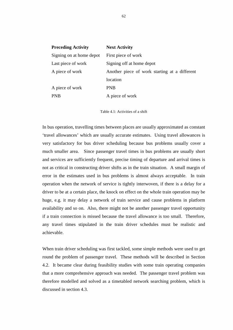
62
Preceding Activity Next Activity
Signing on at home depot First piece of work
Last piece of work Signing off at home depot
A piece of work Another piece of work starting at a different
location
A piece of work PNB
PNB A piece of work
Table 4.1: Activities of a shift
In bus operation, travelling times between places are usually approximated as constant
‘travel allowances’ which are usually accurate estimates. Using travel allowances is
very satisfactory for bus driver scheduling because bus problems usually cover a
much smaller area. Since passenger travel times in bus problems are usually short
and services are sufficiently frequent, precise timing of departure and arrival times is
not as critical in constructing driver shifts as in the train situation. A small margin of
error in the estimates used in bus problems is almost always acceptable. In train
operation when the network of service is tightly interwoven, if there is a delay for a
driver to be at a certain place, the knock on effect on the whole train operation may be
huge, e.g. it may delay a network of train service and cause problems in platform
availability and so on. Also, there might not be another passenger travel opportunity
if a train connection is missed because the travel allowance is too small. Therefore,
any travel times stipulated in the train driver schedules must be realistic and
achievable.
When train driver scheduling was first tackled, some simple methods were used to get
round the problem of passenger travel. These methods will be described in Section
4.2. It became clear during feasibility studies with some train operating companies
that a more comprehensive approach was needed. The passenger travel problem was
therefore modelled and solved as a timetabled network searching problem, which is
discussed in section 4.3.

63
4.2 Simple approaches for tackling passenger travel
4.2.1 Using estimated average travel time
If the service of transport provided is frequent enough (e.g. underground), or if
walking is achievable, like the bus situation, using estimated travel times between
places would seem to be realistic enough for the purpose. This is what IMPACS
usually does when solving bus driver scheduling problems. The main drawback in
using estimates in train problems is that some of the shifts produced may not be
operable. The constant times are applied to the whole day and therefore lack
flexibili ty. During rush hours when the transport service is at the peak, the estimates
may be too slack and result in inefficiency in the shifts. During off peak hours, the
estimates may be too tight or even unachievable because transport service is not
sufficiently frequent. Even if dif ferent constants were to be used according to
different periods of time of the day, it would be difficult to cater for the different
levels of service realistically.
Using estimates is inappropriate for problems which have a non-commuting type
service, e.g. rural, because the service level of these types of service varies greatly
during the day.
4.2.2 Adding artif icial trips
Another way to deal with the problem is to identify any crucial passenger travel trips
and add them to the data as artificial work pieces to be covered. This was used very
often when there were difficulties in covering some of the work because there was no
possible means for essential passenger travel. For example, in Figure 4.2, if a
necessary journey is identified for a driver to travel from C at 2318 arriving D at
2405, this will be added as an extra piece of work:
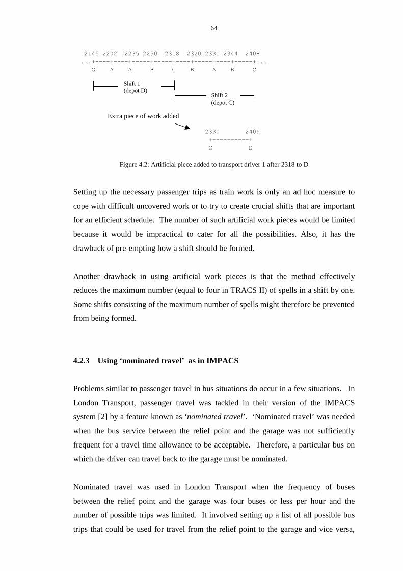
64
2145 2202 2235 2250 2318 2320 2331 2344 2408
...+----+----+-----+-----+----+-----+----+-----+...
G A A B C B A B C
2330 2405
+----------+
C D
Figure 4.2: Artificial piece added to transport driver 1 after 2318 to D
Setting up the necessary passenger trips as train work is only an ad hoc measure to
cope with difficult uncovered work or to try to create crucial shifts that are important
for an efficient schedule. The number of such artificial work pieces would be limited
because it would be impractical to cater for all the possibilities. Also, it has the
drawback of pre-empting how a shift should be formed.
Another drawback in using artificial work pieces is that the method effectively
reduces the maximum number (equal to four in TRACS II) of spells in a shift by one.
Some shifts consisting of the maximum number of spells might therefore be prevented
from being formed.
4.2.3 Using ‘nominated travel’ as in IMPACS
Problems similar to passenger travel in bus situations do occur in a few situations. In
London Transport, passenger travel was tackled in their version of the IMPACS
system [2] by a feature known as ‘nominated travel’. ‘Nominated travel’ was needed
when the bus service between the relief point and the garage was not sufficiently
frequent for a travel time allowance to be acceptable. Therefore, a particular bus on
which the driver can travel back to the garage must be nominated.
Nominated travel was used in London Transport when the frequency of buses
between the relief point and the garage was four buses or less per hour and the
number of possible trips was limited. It involved setting up a list of all possible bus
trips that could be used for travel from the relief point to the garage and vice versa,
Shift 2(depot C)
Extra piece of work added
Shift 1(depot D)

65
together with the walking time required at each end. Whenever the travel time
between the two points was required, for example, to calculate the signing on
allowance at the relief point at a particular time of day, the list was searched to find
the best bus trip.
Nominated travel is an improved and extended way of specifying essential passenger
trips compared to the other two methods described above. It is different from
inserting artificial trips because there is no extra work added to the data. There are a
number of travel possibilities provided instead of just one trip. However, the task of
setting up the list of possible trips is tedious and will be impracticable to extend to all
the relief opportunities.
4.2.4 ‘Overlapping work’ as passenger travel
It is a general property of the set covering problem that schedules produced by the
mathematical process sometimes contain small amounts of work covered by more
than one driver, which is known as ‘overcover’. Overcover occurs when a piece of
work is assigned both to the shift covering the previous piece of work, and to the shift
covering the following piece. In Figure 4.3, from 1145 to 1302 is a piece of over-
covered work. In the bus situation, overcover is more likely to occur when the
scheduler restricts the shift creation process to produce shifts which are individually
efficient but which cannot easily be fitted together without overlapping. Usually, the
scheduler can edit the schedule to remove the overcover piece from one of the shifts
provided the modified shift is still valid.
0615 0732 0843 1017 1145 1302 1435 1550 1718 1920 2031 2144 2301
+----+----+-----+-----+----+-----+----+-----+-------+----+----+----+
G A A B C B C B C A A D G
Figure 4.3: Overcover
Shift 1(depot B)
Shift 2(depot C)
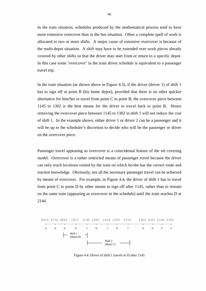
66
In the train situation, schedules produced by the mathematical process tend to have
more extensive overcover than in the bus situation. Often a complete spell of work is
allocated to two or more shifts. A major cause of extensive overcover is because of
the multi-depot situation. A shift may have to be extended over work pieces already
covered by other shifts so that the driver may start from or return to a specific depot.
In this case some ‘overcover’ in the train driver schedule is equivalent to a passenger
travel trip.
In the train situation (as shown above in Figure 4.3), if the driver (driver 1) of shift 1
has to sign off at point B (his home depot), provided that there is no other quicker
alternative for him/her to travel from point C to point B, the overcover piece between
1145 to 1302 is the best means for the driver to travel back to point B. Hence
removing the overcover piece between 1145 to 1302 in shift 1 will not reduce the cost
of shift 1. In the example shown, either driver 1 or driver 2 can be a passenger and it
will be up to the scheduler’s discretion to decide who will be the passenger or driver
on the overcover piece.
Passenger travel appearing as overcover is a coincidental feature of the set covering
model. Overcover is a rather restricted means of passenger travel because the driver
can only reach locations visited by the train on which he/she has the correct route and
traction knowledge. Obviously, not all the necessary passenger travel can be achieved
by means of overcover. For example, in Figure 4.4, the driver of shift 1 has to travel
from point C to point D by other means to sign off after 1145, rather than to remain
on the same train (appearing as overcover in the schedule) until the train reaches D at
2144.
0615 0732 0843 1017 1145 1302 1435 1550 1718 1920 2031 2144 2301
+----+----+-----+-----+----+-----+----+-----+-------+----+----+----+
G A A B C B C B C A A D G
Figure 4.4: Driver of shift 1 travels to D after 1145
Shift 1(depot D)
Shift 2(depot C)
67
4.3 Solving the passenger travel problem
Finding the passenger travel trips from point s to point t involves two similar but
separate problems : a forward search problem and a backward search problem.
Forward search involves finding the earliest arrival time at t and the journey details
leaving at or after a specified start time at location s. Backward search involves
finding the latest departure time from s and the journey details to arrive at t at or
before a specified end time at location t. In both searches, the exact times of train
departure and arrival as in the timetable must be used and enough walking time must
be allowed to change trains.
Passenger travel is a variant of the shortest path problem because it involves working
out the duration of the trip and an itinerary for going from a starting point to a
destination in the quickest way. However the classical shortest path algorithms, e.g.
Dijkstra’s [67], are not directly applicable to the passenger travel problem. These
algorithms deal with finding the shortest distances between two points through a
network. One of the characteristics of the classical shortest path problem is that the
distances between points are always constants although travelling from t to s may be
different from s to t, and may vary depending on the available modes of transport.
In our passenger travel problem, travel times depend on means of transportation
whose availability changes. For example, there may be a connection from s to t, say
departing s at 8 a.m. but the connection between s and t may not exist at 9 a.m. There
may be cases when some travel times can still be represented as constants, for
instance, when the types of travelling involved are predictable, such as walking, or
there is a constant supply of service cars for transportation. When the travel times
vary from time to time, the duration of the trip will depend on the availability of any
transport at the time the trip starts or ends.
From our experience on various train problems, the majority of the drivers’ passenger
travel is by train or service car or regular taxis rides provided by their own operating
company. There are occasions when the driver may travel on vehicles operated by
other public transport operating companies. In order to construct the required
68
passenger travel trips, not only all the arrival and departure times of the trains in the
existing problem must be present, but any additional trips that are not in the problem
may be used as means for transportation have to be provided in the data. It is
important that possible passenger trips should not be mixed with the train work to be
scheduled, because the latter work must be allocated to a driver, while passenger trips
are simply available if required. A new algorithm is developed in this research that is
designed mainly for finding passenger travel trips for train problems. The resulting
software also acts as a pre-processor which separates train work to be scheduled from
trips that are purely for passenger travel. The algorithm will be described in Section
4.3.5. The next section will describe some related work on this type of problem. In
order to present a clear illustration of the problem, it is necessary to devise some
terminology and notations and they are introduced in Section 4.3.2.
4.3.1 Related work
There are many published works on the classical Shortest Path problems, and for an
overview of these algorithms, see for instance: Deo and Pang [68], Golden[69] van
Vliet[70]. However none of these algorithms could be used for searching the shortest
path in a timetabled network. The most recent publications directly relevant to the
passenger travel problem is described by Tulp and Siklossy [71, 72].
Tulp and Siklossy describe the DYNET search algorithm for finding optimal paths in
a timetabled network. DYNET is implemented in a system called TRAINS which
searches the entire Dutch railway services network. The system is being used by the
general public at the information centres of the Dutch railway company to answer a
user’s query.
Tulp et al propose a discrete dynamic network to represent a timetabled service
network. In this discrete dynamic network, there are only finite, discrete and
predetermined possibilities for moving from one node to another. The discrete
dynamic network contains two parts. The first part is a finite directed graph of
vertices and a set of directed edges joining two vertices. The second part contains the
minimum connection times (directional) when changing trains at the vertices. The
search algorithm DYNET is based on the Dijkstra’s algorithm, Dijk, with substantial

69
modifications to cater for the discrete nature and the variable connection times at
vertices. The algorithm contains a forward search which finds the earliest arrival
time at t from s and a backward search which uses the results of the forward search, to
find the latest departure time from s to arrive at t.
4
DYNET can search a comprehensive network and finds a journey with many different
journey legs. The search algorithm is made more efficient by using several
techniques, e.g. avoiding needless edges, eliminating small stations, introducing lower
bounds and using an abstraction space to narrow down the search area. However, the
model used here does not cater for possible walking between places which can be
added at the beginning, in between or at the end of the train journey. The search is on
the train service and there is no mention of integrating other public transport services
into the problem. In our passenger travel problem, walking between places and using
other means of transport have to be taken into account when searching for the
quickest path. Hence the DYNET algorithm cannot be directly applicable to our
situation without some modifications.
(Sections 4.3.2 to 4.3.5.2 inclusive are withheld due to Intellectual Property
Rights)

79
4.4 Travel information produced from TRAVEL
The algorithm described in the previous section has been implemented in C++ and the
program is called ‘TRAVEL’. Since the shift creation process is complex, it will
simplify the shift creation algorithm if the passenger travel process is separated from
the shift creation process. Hence all the possible passenger travel information has to
be available before the shift creation process starts. TRAVEL produces three files:
1. a data file of the problem with all the travel opportunities which are not relief
opportunities removed;
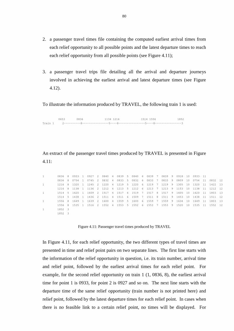
80
2. a passenger travel times file containing the computed earliest arrival times from
each relief opportunity to all possible points and the latest departure times to reach
each relief opportunity from all possible points (see Figure 4.11);
3. a passenger travel trips file detailing all the arrival and departure journeys
involved in achieving the earliest arrival and latest departure times (see Figure
4.12).
To illustrate the information produced by TRAVEL, the following train 1 is used:
0653 0836 1134 1216 1514 1556 1852
Train 1 2----------8----------------5----8----------------5----8----------------3
An extract of the passenger travel times produced by TRAVEL is presented in Figure
4.11:
1 0836 8 0933 1 0927 2 0840 4 0839 5 0840 6 0839 7 0839 9 0918 10 0933 11
0836 8 0754 1 0745 2 0832 4 0833 5 0832 6 0833 7 0833 9 0809 10 0754 11 0832 12
1 1216 8 1320 1 1245 2 1220 4 1219 5 1220 6 1219 7 1219 9 1305 10 1320 11 1422 13
1216 8 1138 1 1136 2 1212 4 1213 5 1212 6 1213 7 1213 9 1153 10 1138 11 1212 12
1 1514 5 1620 1 1609 2 1517 4 1517 6 1519 7 1517 8 1517 9 1605 10 1620 11 1803 13
1514 5 1438 1 1436 2 1511 4 1511 6 1509 7 1511 8 1511 9 1453 10 1438 11 1511 12
1 1556 8 1649 1 1639 2 1600 4 1559 5 1600 6 1559 7 1559 9 1634 10 1649 11 1803 13
1556 8 1535 1 1516 2 1552 4 1553 5 1552 6 1553 7 1553 9 1520 10 1535 11 1552 12
1 1852 3
1852 3
Figure 4.11: Passenger travel times produced by TRAVEL
In Figure 4.11, for each relief opportunity, the two different types of travel times are
presented in time and relief point pairs on two separate lines. The first line starts with
the information of the relief opportunity in question, i.e. its train number, arrival time
and relief point, followed by the earliest arrival times for each relief point. For
example, for the second relief opportunity on train 1 (1, 0836, 8), the earliest arrival
time for point 1 is 0933, for point 2 is 0927 and so on. The next line starts with the
departure time of the same relief opportunity (train number is not printed here) and
relief point, followed by the latest departure times for each relief point. In cases when
there is no feasible link to a certain relief point, no times will be displayed. For
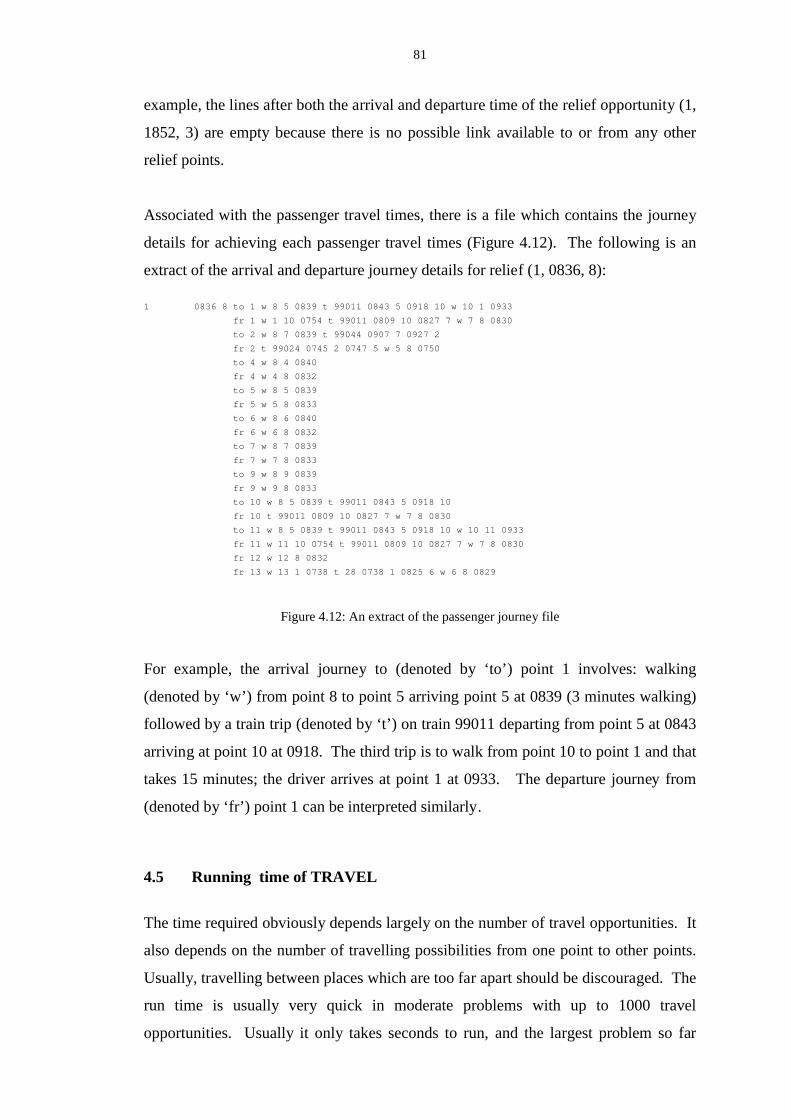
81
example, the lines after both the arrival and departure time of the relief opportunity (1,
1852, 3) are empty because there is no possible link available to or from any other
relief points.
Associated with the passenger travel times, there is a file which contains the journey
details for achieving each passenger travel times (Figure 4.12). The following is an
extract of the arrival and departure journey details for relief (1, 0836, 8):
1 0836 8 to 1 w 8 5 0839 t 99011 0843 5 0918 10 w 10 1 0933
fr 1 w 1 10 0754 t 99011 0809 10 0827 7 w 7 8 0830
to 2 w 8 7 0839 t 99044 0907 7 0927 2
fr 2 t 99024 0745 2 0747 5 w 5 8 0750
to 4 w 8 4 0840
fr 4 w 4 8 0832
to 5 w 8 5 0839
fr 5 w 5 8 0833
to 6 w 8 6 0840
fr 6 w 6 8 0832
to 7 w 8 7 0839
fr 7 w 7 8 0833
to 9 w 8 9 0839
fr 9 w 9 8 0833
to 10 w 8 5 0839 t 99011 0843 5 0918 10
fr 10 t 99011 0809 10 0827 7 w 7 8 0830
to 11 w 8 5 0839 t 99011 0843 5 0918 10 w 10 11 0933
fr 11 w 11 10 0754 t 99011 0809 10 0827 7 w 7 8 0830
fr 12 w 12 8 0832
fr 13 w 13 1 0738 t 28 0738 1 0825 6 w 6 8 0829
Figure 4.12: An extract of the passenger journey file
For example, the arrival journey to (denoted by ‘to’ ) point 1 involves: walking
(denoted by ‘w ’) f rom point 8 to point 5 arriving point 5 at 0839 (3 minutes walking)
followed by a train trip (denoted by ‘t’ ) on train 99011 departing from point 5 at 0843
arriving at point 10 at 0918. The third trip is to walk from point 10 to point 1 and that
takes 15 minutes; the driver arrives at point 1 at 0933. The departure journey from
(denoted by ‘f r’) point 1 can be interpreted similarly.
4.5 Running time of TRAVEL
The time required obviously depends largely on the number of travel opportunities. It
also depends on the number of travelling possibilities from one point to other points.
Usually, travelling between places which are too far apart should be discouraged. The
run time is usually very quick in moderate problems with up to 1000 travel
opportunities. Usually it only takes seconds to run, and the largest problem so far
82
with more than 3,000 travel opportunities took less than fifteen minutes on a 333MHz
Pentium II personal computer.
It is envisaged that if there is a requirement to increase the number of train trips to
more than two, the run time will be expected go to up by at least half of original run
time.
4.6 Comparison of results with early case studies
In the case studies conducted in the early stage of the research, TRAVEL was not
available. Passenger travel in these case studies was dealt with by using estimated
travel times and some artificial work pieces as the stipulated travelling. These case
studies are: East Coast Main Line (EC), Thameslink (TL), and Regional Railways
North East (Heaton). There are two separate exercises for Thameslink, one is TL95
which is based on the company’s conditions at the time of the exercise; the other is
TL96. TL96 involves investigating some ‘what-if’ scenarios in one of which a
location at the centre of London is not to be used as a driver relief point. The data of
TL96 is largely different from TL95 because it is based on different train schedules.
The case studies will be described more fully in Chapter Six.
Estimated travel times and artificial work pieces as passenger travel were used in the
EC, TL96 and Heaton problems whereas only estimated travel times were used in the
TL95 problem.
The problems in these case studies were re-run making use of the TRAVEL program
to achieve precise passenger travel. Table 4.2 compares the best schedules produced
by using the passenger travel method against schedules produced not using this
method. For fair comparison, the same conditions applied in each case, i.e. same set
of parameters and programs.
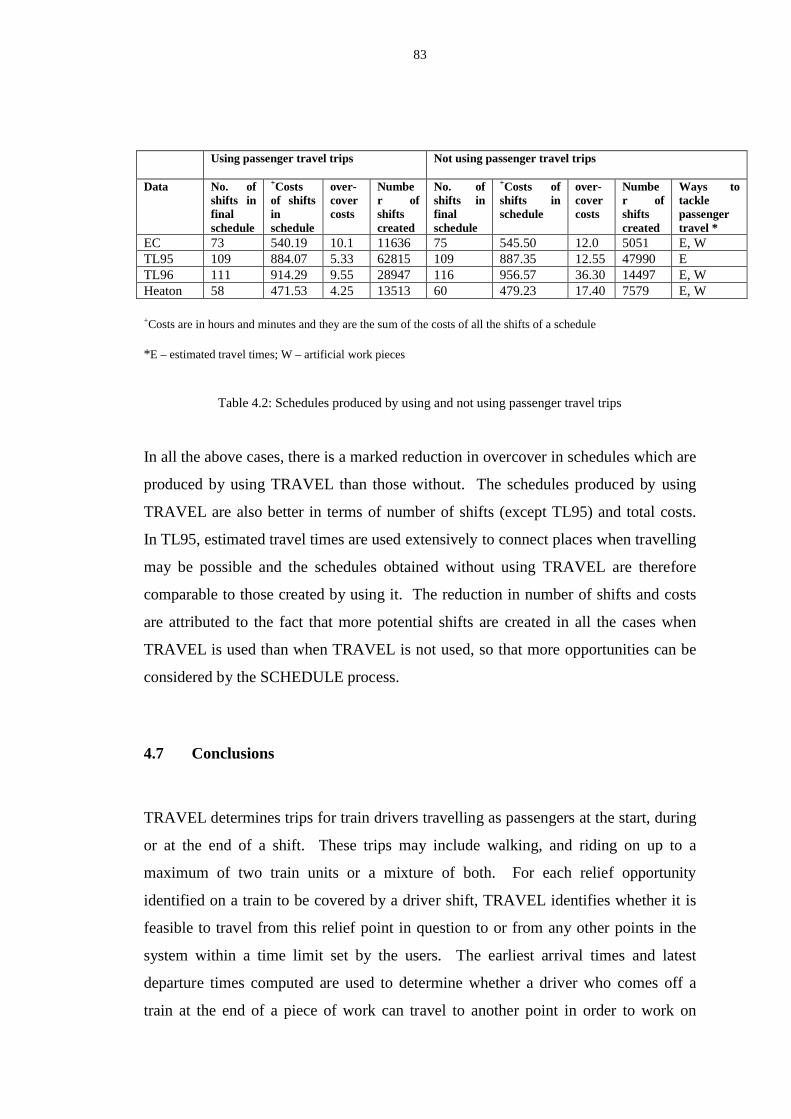
83
Using passenger travel tri ps Not using passenger travel tri ps
Data No. ofshifts infinalschedule
+Costsof shiftsinschedule
over-covercosts
Number ofshiftscreated
No. ofshifts infinalschedule
+Costs ofshifts inschedule
over-covercosts
Number ofshiftscreated
Ways totacklepassengertravel *
EC 73 540.19 10.1 11636 75 545.50 12.0 5051 E, WTL95 109 884.07 5.33 62815 109 887.35 12.55 47990 ETL96 111 914.29 9.55 28947 116 956.57 36.30 14497 E, WHeaton 58 471.53 4.25 13513 60 479.23 17.40 7579 E, W
+Costs are in hours and minutes and they are the sum of the costs of all the shifts of a schedule
*E – estimated travel times; W – artificial work pieces
Table 4.2: Schedules produced by using and not using passenger travel trips
In all the above cases, there is a marked reduction in overcover in schedules which are
produced by using TRAVEL than those without. The schedules produced by using
TRAVEL are also better in terms of number of shifts (except TL95) and total costs.
In TL95, estimated travel times are used extensively to connect places when travelling
may be possible and the schedules obtained without using TRAVEL are therefore
comparable to those created by using it. The reduction in number of shifts and costs
are attributed to the fact that more potential shifts are created in all the cases when
TRAVEL is used than when TRAVEL is not used, so that more opportunities can be
considered by the SCHEDULE process.
4.7 Conclusions
TRAVEL determines trips for train drivers travelling as passengers at the start, during
or at the end of a shift. These trips may include walking, and riding on up to a
maximum of two train units or a mixture of both. For each relief opportunity
identified on a train to be covered by a driver shift, TRAVEL identifies whether it is
feasible to travel from this relief point in question to or from any other points in the
system within a time limit set by the users. The earliest arrival times and latest
departure times computed are used to determine whether a driver who comes off a
train at the end of a piece of work can travel to another point in order to work on

84
another train, or to sign off, or to have a mealbreak. It is also possible to specify a
‘leeway’ figure to allow the user to adjust a global late running.
TRAVEL has been tested and used extensively in all the case studies carried out in
this research. Before TRAVEL was available, it was difficult to ascertain that the
schedules produced were all operable in real life in terms of travelling. TRAVEL has
contributed a major improvement towards solving train driver scheduling problems
and the resulting driver schedules are much more realistic and operable than those
produced by previous efforts.
85
Chapter Five
Building potential shifts
5.1 Introduction
The first phase of TRACS II generates a set of valid potential good shifts which must
satisfy conditions in the union agreements, and within such constraints aims at
covering all the train work. While the number of shifts constructed must not be
excessive, it is important to ensure that no shifts vital to an efficient schedule are
omitted. At the early stage of this research, a slightly modified IMPACS was used in
several short studies of train problems. The shift generation process of IMPACS,
known as GEN, used some heuristics specifically designed for the bus driver
scheduling problems. Since bus driver scheduling problems are generally simpler
than train problems, some fundamental changes to the GEN process were needed to
cope with the more complex train situation. A brief description of the shift generation
process in IMPACS will be outlined in this chapter, which is followed by a list of
difficulties identified when applying GEN for train problems. The shift generation
process was therefore designed afresh for the train situation. The new approach will
be discussed in detail. Finally, this chapter will give a brief account of the other
processes in TRACS II .
86
5.2 Outline of the shift generation process in IMPACS
GEN first sorts all work pieces in ascending order of start times. It then forms two-
spell shifts with a mealbreak in between the spells, followed by forming three-spell
shifts.
The first spell of a two spell shift is formed by selecting a pair of relief opportunities
in a bus graph (or known as running board), such that the work in between the pair of
relief opportunities forms a valid spell according to the parameters governing its
legality. The mealbreak will start at the end of the first spell. In choosing the next
spell after a mealbreak, the process will first choose the spell that gives rise to the
shortest valid mealbreak. The second spell will end at the earliest relief time which
will give a second stretch at least as long as it is allowed by the parameters. This will
form a potential shift.
The shift is then validated by checking against any parameters for this shift type
which cannot be checked earlier. There is also a special routine used for checking the
validity of the shift according to some specific rules of individual companies. If the
shift is not valid, then either the second stretch is extended to the next relief time, or
other second stretches with later starting times are considered. If the shift is valid, the
next step depends on whether the company in question has a ‘minimum paid time’
policy. Many agreements specify a minimum paid time of say 8:30 hours for a day’s
work; any shift which would otherwise cost less than this is paid the minimum paid
time. If such a condition exists and the shift in question costs less than the minimum
paid day, the process will try to extend the end of the second stretch to the next relief
time without becoming invalid or exceeding the minimum paid day. The shift with a
shorter length but costing the same as the longer shift will be discarded. After a valid
shift has been found, the process will try to extend the finishing times on the second
stretch to form other valid shifts until no further valid shifts can be formed. The
process then chooses the next available spell (later starting times for the second
stretch) to combine with the same first spell to form the next valid shift and so on.
Since the potential number of combinations can be enormous, the process will only
consider a certain number of second spells with different starting times to match with
the same first spell. This is also controlled by parameter. When all possible second
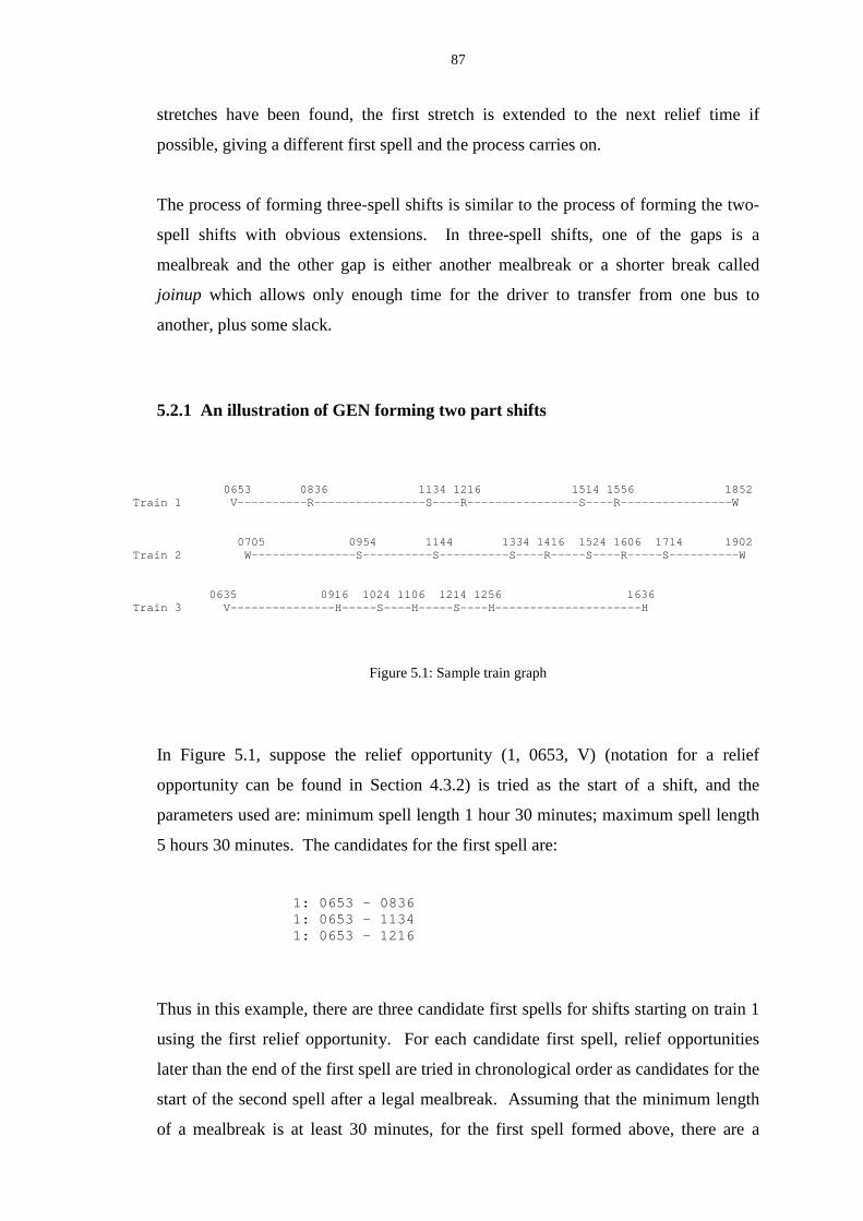
87
stretches have been found, the first stretch is extended to the next relief time if
possible, giving a different first spell and the process carries on.
The process of forming three-spell shifts is similar to the process of forming the two-
spell shifts with obvious extensions. In three-spell shifts, one of the gaps is a
mealbreak and the other gap is either another mealbreak or a shorter break called
joinup which allows only enough time for the driver to transfer from one bus to
another, plus some slack.
5.2.1 An illustration of GEN forming two part shifts
0653 0836 1134 1216 1514 1556 1852 Train 1 V----------R----------------S----R----------------S----R----------------W
0705 0954 1144 1334 1416 1524 1606 1714 1902 Train 2 W---------------S----------S----------S----R-----S----R-----S----------W
0635 0916 1024 1106 1214 1256 1636 Train 3 V---------------H-----S----H-----S----H---------------------H
Figure 5.1: Sample train graph
In Figure 5.1, suppose the relief opportunity (1, 0653, V) (notation for a relief
opportunity can be found in Section 4.3.2) is tried as the start of a shift, and the
parameters used are: minimum spell length 1 hour 30 minutes; maximum spell length
5 hours 30 minutes. The candidates for the first spell are:
1: 0653 - 08361: 0653 - 11341: 0653 - 1216
Thus in this example, there are three candidate first spells for shifts starting on train 1
using the first relief opportunity. For each candidate first spell, relief opportunities
later than the end of the first spell are tried in chronological order as candidates for the
start of the second spell after a legal mealbreak. Assuming that the minimum length
of a mealbreak is at least 30 minutes, for the first spell formed above, there are a
88
number of second spells that can be combined with the first spell to form a potential
shift:
1:0653 – 0836 -> 3:0916 - 1106 -> 3:0916 - 1214 -> 3:0916 - 1256 -> 2:0954 - 1144 -> 2:0954 - 1334
and so on
The process does not store information on any spells that have been formed before or
used in a valid shift and the same spell of work may be validated against the same set
of parameters over and over again.
5.2.2 Five types of shifts formed by GEN
GEN first forms all the possible two-spell shifts according to each of the following
shift types and in the following order and then forms all the possible three-spell shifts
in a similar way:
1. EARLY shifts are shifts taking buses out of the garage before the morning peak;
2. LATE shifts are shifts working on late evening buses returning to the garage;
3. SPLIT shifts are basically shifts with a long spreadover and a long mealbreak;
4. DAY shifts are shifts which either take over early buses on the road from another
crew, or occasionally take a later-starting bus out of the garage;
5. MIDDLE shifts are shifts which either finish at the garage shortly after the
evening peak, or hand over to late duties on the road.
Except early shifts, the other types of shifts can start at any time as specified in the
parameters, and not just at the start of a bus graph. Day and middle shifts, however,

89
must start at a relief time which has been used as a finishing time for a spell of work
in a shift already formed, unless they start at the beginning of a bus graph.
The shift generation process in IMPACS was modified, in the following ways among
others to cope temporarily with the train problems:
1. Valid shifts are sub-classified according to their length of spreadover in addition
to the five different types;
2. Shifts starting at one depot must finish at the same depot in order to cater for
multi-depot situations.
Since the aim of the 1990 BR project was to create a model which could predict the
number of shifts required, the above modifications were adequate to achieve this goal.
5.3 Diff iculties of using GEN in the train situation
The heuristics built in GEN were very specific to the bus problems. Some of the
heuristics were designed to cut down the number of potential shifts generated sensibly
because the computers’ memory and processing power in the early 80’s were
expensive and much less powerful than they are now. Other heuristics were to
simulate the methods manual schedulers used for constructing a schedule. When
GEN was used in the train situations, some of the heuristics which are not designed
for the train situation had prevented some crucial shifts from being formed. The
following are a list of difficulties identified:
1. GEN classifies shifts into five different types as above and then generates shifts
according to the characteristics of each type. In train operations, such
classifications are less relevant because their daily operations are usually longer
than those in bus situations. For instance, they may start very early in the morning
or finish very late at night or operate round-the-clock. Instead, the classification
of shifts according to their spreadover is more useful. This is because there used
90
to be rules in the union agreement governing the proportion of shifts with long
spreadover in the schedules.
2. The heuristic which guides the process to form Middle and Day shifts may
prohibit some crucial shifts from being generated in the train situation. GEN
creates two spell shifts first and then follows by three spell shifts. In each stage,
similar heuristics are used to form shifts. Some criteria used in these processes
only consider the shifts that have been formed by that time. For example, Day
and Middle shifts must start at a relief time which has already been used as a
finishing time by a portion of a shift already formed unless they start at depots.
Since three spell shifts are generated later, GEN prevents some critical two spell
Middle or Day shifts from being formed because they use a relief time which has
not yet been used as a finishing time by a yet to be formed three-spell shift.
3. When ‘minimum paid time’ policy is in operation, shorter shifts that cost the same
as the longer ones and are contained within them are discarded regardless of their
home depots. However, in a multi-depot situation, these shorter shifts cannot be
discarded if they do not belong to the same depot as the longer ones.
4. After a first spell is formed, the process will only consider a certain number of
second spells with different starting times to match with the same first spell. The
number is controlled by a parameter and the consequence is that no matter how
slack the other parameters are they are ineffective in allowing more shifts to be
formed. This coupled with situations when there are many relief times close
together, e.g. in an intensive urban situation, could lead to problems in forming
enough shifts of the certain desired characteristics.
5. The GEN process generates shifts that can contain up to three spells of work (also
known as three part shifts). In train operation, some of the work pieces are very
fragmented (e.g. shunting or re-platforming) and hence there is a need to create
shifts with more than three spells of work.
6. There are a lot of repeated checks on the same spell of work during the shift
generation process because any valid spells that have been validated before are not

91
stored. The same applied when the process is forming valid stretches to match
with a first spell.
In addition to the above list, there are many new requirements specific to the train
situation that GEN could not meet without a major change in the approach, it was
decided that a completely new approach was needed.
(Section 5.4 and its sub-sections are withheld due to Intellectual Property Rights)
110
5.5 Running time of the shift generation process
The new method described here has been implemented in C++ and the program is
called ‘BUILD’. The running time of BUILD depends largely on the number of
spells and stretches that can be formed, which in turn depends on the number of relief
opportunities in the problem and the slackness of the parameters. The processes of
forming spells and stretches are very quick compared to the process of shift
formation. The process may take a significant amount of computer time for problems
with more than 700 relief opportunities. It may take up to two hours to run such a
problem on a 333 MHz Pentium II personal computer. For smaller problems with less
than 500 relief opportunities, the process usually takes less than 30 minutes. The
number of depots present in the problem will also affect the run time of the process.
This is because if the work of the shift can be done by more than one depot, the
version of the shift for each valid depot has to be formed beforehand in order to
determine which depot gives the lowest cost.
The run time depends also on how soon invalid shifts can be rejected. The presence
of route and traction knowledge can help to cut down the run time since they limit the
choices of depot and also the combinations of pieces of work to form spells, stretches
or shifts.
5.6 Uncovered work
Sometimes BUILD may leave some work uncovered. This may be due to errors in
the data, or it may be possible that parameters used were deliberately chosen which
have sensibly prevented too many inefficient shifts from having been created, but
have prevented some necessary shifts. BUILD allows for a re-run aiming to cover
this uncovered work based on a revised parameter file which has been slackened and
it will only create shifts which cover the previously uncovered work.
111
5.7 Parallel building of shifts
When there is a wide variability in the type of shift to be used, sometimes it is best to
use the shift generating process several times with different parameter ranges
appropriate to the types of shifts being generated. For example, when exercises are
being carried out with shift lengths ranging from four to eleven hours. In this case, it
is sensible to run the process once on each of a set of smaller ranges, using different
soft parameters to restrict the generation of inappropriate shifts. For example, in
generating shifts between nine and eleven hours one might sensibly rule out any shifts
with less than five hours driving; shifts between four and six hours might be restricted
from having less than 2.5 hours driving.
4
Another example is to encourage the creation of as many two spell shifts as possible
while tightening the parameters for forming three and four spells shifts. This can be
done by using very slack parameters for generating two spell shifts only and using
very tight parameters to create three and four spells shifts. The reason for creating
more two spells shifts than any other type is that two spells shifts are usually more
efficient than three and four spells. Also, two spell shifts can help to simplify the ILP
in the shift selection process because more two spell shifts will result in fewer work
piece constraints (rows).
5.8 Refinement of the sets of potential shifts created by BUILD
The two processes described here are for refining the sets of potential shifts created by
one or several BUILD runs before they are presented to the shift selection process.
The processes are the work of another member of the SACM group but are briefly
introduced here for completeness.
5.8.1 Reduction of the shift set - Program SIEVE
After the shift generation process, a process, SIEVE can be used to eliminate in a
logical manner some of the less efficient shifts formed. SIEVE discards shifts in one
or a combination of the following ways:

112
(i) Eliminate duplicated copies of the same shifts.
(ii) Compare a shift with all other shifts to form a pair and eliminate the ‘redundant’
shift regardless of whether the cost of the eliminated shift is cheaper than the
other. A ‘r edundant’ shift is one which is entirely contained in another shift or
shifts.
(iii) Compare a shift with all other shifts to form a pair and only eliminate the
‘redundant’ shift if the eliminated shift is cheaper than the other.
(iv) Eliminate relatively inefficient shifts which only contain work which is covered
by many other possible shifts.
The above ways of discarding shifts are presented in a menu format for the users to
choose. Users can choose one or more ways to remove some potential shifts.
Except (i), all the other three ways discard shifts regardless of the depots to which
they belong. Therefore, there is a risk of getting rid of shifts belonging to one depot,
say depot A, because the work may have already been covered by more efficient
shifts which belong to a different depot. Hence there is a potential risk that crucial
shifts in forming efficient schedules may be discarded. The problem is worsened
when there is a limit on the number of shifts of a particular depot, a shift discarded
might become an essential shift in order to satisfy the constraint.
5.8.2 Combining dif ferent potential shift sets – program MERGE
This module is required only if BUILD has been used several times, e.g. there is a
need for a second run to cover work that had previously been left. It is designed to
combine the results of several (up to nine) separately generated sets of shifts, after
they have passed through the SIEVE process. MERGE can merge up to a total of
120,000 shifts and 9 different problems. The resultant combined set of shifts is
examined to remove any duplication, whether this occurred by merging sets, or was
present in one of the individual sets.

113
5.9 Shift selection using Integer Linear Programming – Process SCHEDULE
This phase employs the set covering integer linear programming model [3, 4] to select
from a large shift set the most economical subset (the schedule) that covers all the
work and satisfies any other constraints present. It was originally developed in the
1970s [73], but has since undergone several phases of significant revision and
enhancement. Since the development of TRACS II , the program has been
restructured and brought up-to-date. The author contributed in tailoring it to handle
train driver scheduling problems in 1994. Since then, Willers[8] and Fores[9] have
improved the mathematical process using new methods, and their recent
improvements to the algorithm will be briefl y described in Chapter Seven.
If a solution is found, a print program will be used to format the solution in a readable
format.
5.10 Conclusions
The two processes TRAVEL and BUILD described in the last and present chapters
fulfil the objective of producing schedules of good quality acceptable to train
operating companies (see Chapter for the results of various applications). The results
are reflected in:
1. A new driver shift generation process.
2. A new pre-processor for computing precise travelling possibilities for train
drivers.
3. Enriched data input now accurately describing scheduling conditions.
These achievements encompass many requirements in train driver scheduling that had
not been encountered before in bus driver scheduling.
114
Chapter Six
Applications and implementation of
TRACS II
6.1 Introduction
TRACS II has been used on behalf of about a dozen train operators (Section 6.2) and
on a number of bus operators (Section 6.3) since the start of this research. The
processes TRAVEL and BUILD evolved over this period of time when new and more
complex requirements arose in different problem instances. Table 6.10 shows when
the new features are gradually added to the two processes over the years. The
complexity of the problems has varied considerably reflecting the wide range of
conditions of the train operating companies. The file defining the labour scheduling
rules now contains a wide range of parameters so that most features which are likely
to vary between organisations can readily be defined. However, some organisations
have rules which cannot easily be defined by generic parameters and have to be
handled by specially written code. In general, the amount of such tailoring for
individual companies is limited and can be coded very easily. There are two
publications [74, 75] by the author and colleagues describing the applications of
TRACS II in the context of train driver scheduling.
TRACS II has also been applied in bus driver scheduling problems. The bus
problems are almost always simpler than the train situation, hence the application of
TRACS II to bus problems is more straightforward than to train problems. This
chapter describes the applications of TRACS II to both train and bus operating
companies.
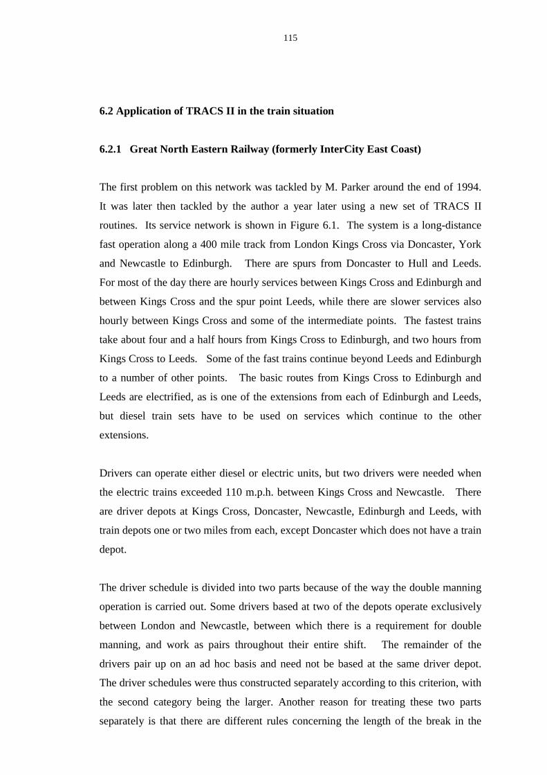
115
6.2 Application of TRACS II in the train situatio n
6.2.1 Great North Eastern Railway (formerly Inter City East Coast)
The first problem on this network was tackled by M. Parker around the end of 1994.
It was later then tackled by the author a year later using a new set of TRACS II
routines. Its service network is shown in Figure 6.1. The system is a long-distance
fast operation along a 400 mile track from London Kings Cross via Doncaster, York
and Newcastle to Edinburgh. There are spurs from Doncaster to Hull and Leeds.
For most of the day there are hourly services between Kings Cross and Edinburgh and
between Kings Cross and the spur point Leeds, while there are slower services also
hourly between Kings Cross and some of the intermediate points. The fastest trains
take about four and a half hours from Kings Cross to Edinburgh, and two hours from
Kings Cross to Leeds. Some of the fast trains continue beyond Leeds and Edinburgh
to a number of other points. The basic routes from Kings Cross to Edinburgh and
Leeds are electrified, as is one of the extensions from each of Edinburgh and Leeds,
but diesel train sets have to be used on services which continue to the other
extensions.
Drivers can operate either diesel or electric units, but two drivers were needed when
the electric trains exceeded 110 m.p.h. between Kings Cross and Newcastle. There
are driver depots at Kings Cross, Doncaster, Newcastle, Edinburgh and Leeds, with
train depots one or two miles from each, except Doncaster which does not have a train
depot.
The driver schedule is divided into two parts because of the way the double manning
operation is carried out. Some drivers based at two of the depots operate exclusively
between London and Newcastle, between which there is a requirement for double
manning, and work as pairs throughout their entire shift. The remainder of the
drivers pair up on an ad hoc basis and need not be based at the same driver depot.
The driver schedules were thus constructed separately according to this criterion, with
the second category being the larger. Another reason for treating these two parts
separately is that there are different rules concerning the length of the break in the

116
middle of the shift when there are two drivers compared with just one. These two
parts are tackled separately and independently.
KingsCross
Doncaster
Leeds
York Newcastle
Edinburgh
Hull
Glasgow
Aberdeen
Figure 6.1: The Great North Eastern Railway network (portion)
In order to produce a schedule where drivers team up on an arbitrary basis it is
necessary to specify all the train work requiring double manning twice and to regard
the shifts produced as totally independent of each other. Double manning is only
required for the wheel turning part of the shift; two drivers are not required for
preparing the train unit before the journey or for ensuring that the unit is left in a safe
manner at the conclusion of the journey.
This problem involves a large geographic area with the opportunities to relieve drivers
remotely spaced both in time and distance. As a result, the problem is small in terms
of number of relief opportunities present in the data. There is no traction restriction in
the problem. Route knowledge is very simple and route restriction applies to a very
small local section of the routes around some depots. This can be ignored for the
purpose of this exercise.
Since this was the first exercise tackled in this research, a lot of the features specific
to the rail problem had not been implemented. Fortunately, some of these features are
not present in the GNER problem, for example, traction knowledge. Passenger travel
is tackled by means of shifts overcover. The shift formation process is
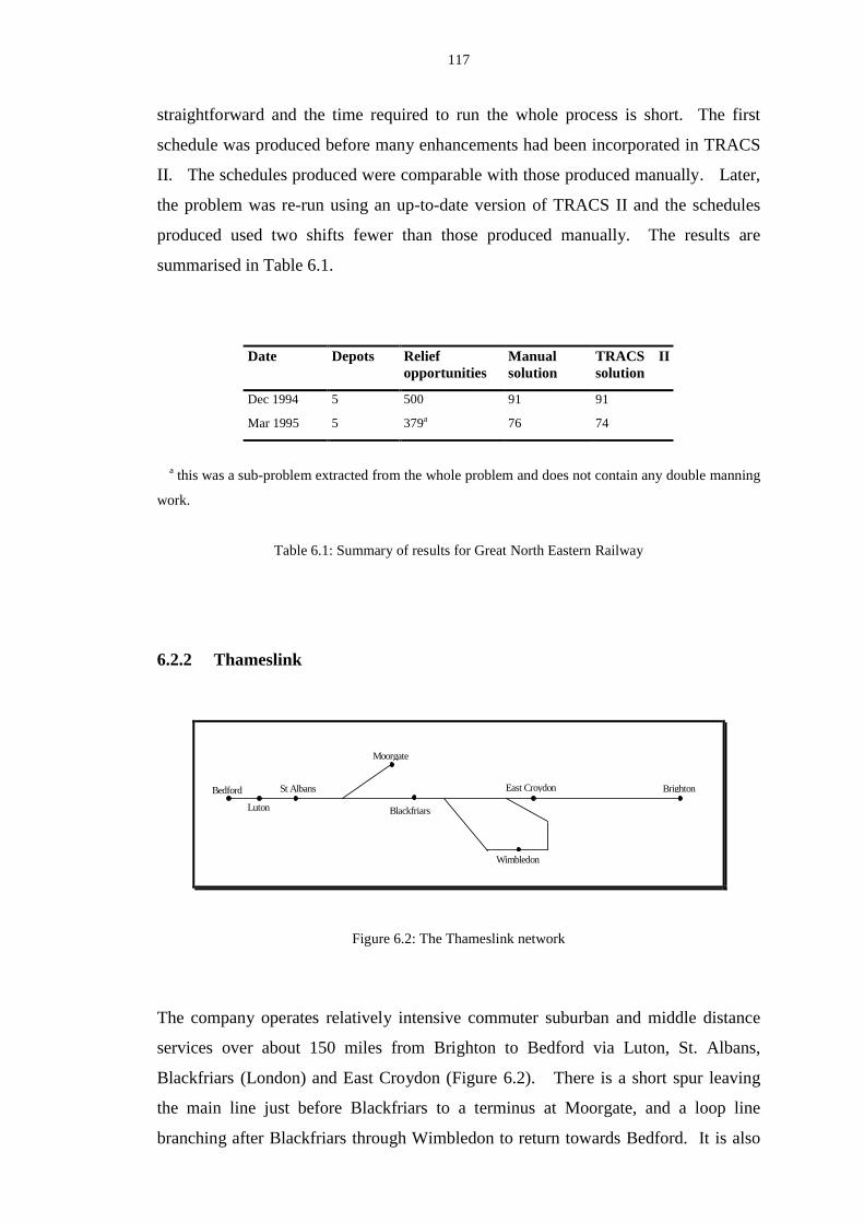
117
straightforward and the time required to run the whole process is short. The first
schedule was produced before many enhancements had been incorporated in TRACS
II. The schedules produced were comparable with those produced manually. Later,
the problem was re-run using an up-to-date version of TRACS II and the schedules
produced used two shifts fewer than those produced manually. The results are
summarised in Table 6.1.
Date Depots Reliefopportunities
Manualsolution
TRACS IIsolution
Dec 1994 5 500 91 91
Mar 1995 5 379a 76 74
a this was a sub-problem extracted from the whole problem and does not contain any double manning
work.
Table 6.1: Summary of results for Great North Eastern Railway
6.2.2 Thameslink
Blackfriars
East Croydon
Wimbledon
Brighton
Moorgate
St Albans
Luton
Bedford
Figure 6.2: The Thameslink network
The company operates relatively intensive commuter suburban and middle distance
services over about 150 miles from Brighton to Bedford via Luton, St. Albans,
Blackfriars (London) and East Croydon (Figure 6.2). There is a short spur leaving
the main line just before Blackfriars to a terminus at Moorgate, and a loop line
branching after Blackfriars through Wimbledon to return towards Bedford. It is also

118
the only surface train operator with a direct link between north and south London
through the commercial heart of the City. The running time from end to end is about
140 minutes, and there are trains about every 15 minutes over the central section.
There are three driver and train depots at Bedford and Brighton, and also at Selhurst
which is near to East Croydon. Selhurst depot is not directly on their service
network. To get to or from Selhurst, drivers have to travel as passengers on trains of
another company unless they are driving to or from the Selhurst depot. Drivers from
Brighton cannot drive between St Albans and Bedford, while drivers from Selhurst
cannot drive between East Croydon and Brighton.
Similar to the GNER exercise, this exercise was tackled before the passenger
travelling, route and traction knowledge features were incorporated. Drivers’ travel
times between relief points were estimated and put into a table of ‘standard’
allowances. While these allowances may be realistic during usual commuting hours
they may become impracticable during late night or early morning hours when the
train service is infrequent. Route knowledge was simple and was coded into the shift
generation process as hard rules. This is a larger problem than the GNER in terms of
number of relief opportunities and number of shifts.
Data received in autumn, 1994 was based on a draft train schedule in 1994. A
schedule was first produced in November, 1994. There were a few amendments to
the data subsequently, which were mostly related to the travel time allowances. By
March, 1995, TRACS II produced a solution with 109 shifts. There was no manual
solution available for direct comparison because the draft train schedule had been
changed significantly by the time the results appeared. The manual solution was
therefore based on a very different set of data. However, the company viewed
TRACS II as a powerful tool for assessing ‘what-if’ scenarios. In Spring 1995
Thameslink supplied us with their latest May 1995 train schedule and requested our
assistance in assessing a few ‘what-if’ scenarios based on the new set of data. The
base data was run fi rst for calibrating purposes with the manual schedule which had
115 shifts. Thameslink wanted to assess the impact on the driver schedule if one or
more or their present crew depots were closed. TRACS II was able to produce a
range of solutions involving ‘no change’, greater or lesser use of individual depots, or
total withdrawal from non-Thameslink depots. On the base scenario where there was
no change in conditions, TRACS II initiall y produced a solution with one shift fewer
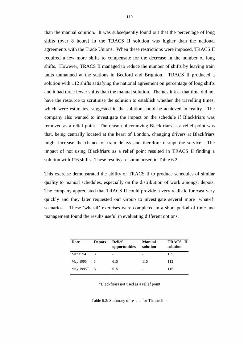
119
than the manual solution. It was subsequently found out that the percentage of long
shifts (over 8 hours) in the TRACS II solution was higher than the national
agreements with the Trade Unions. When these restrictions were imposed, TRACS II
required a few more shifts to compensate for the decrease in the number of long
shifts. However, TRACS II managed to reduce the number of shifts by leaving train
units unmanned at the stations in Bedford and Brighton. TRACS II produced a
solution with 112 shifts satisfying the national agreement on percentage of long shifts
and it had three fewer shifts than the manual solution. Thameslink at that time did not
have the resource to scrutinise the solution to establish whether the travelling times,
which were estimates, suggested in the solution could be achieved in reality. The
company also wanted to investigate the impact on the schedule if Blackfriars was
removed as a relief point. The reason of removing Blackfriars as a relief point was
that, being centrally located at the heart of London, changing drivers at Blackfriars
might increase the chance of train delays and therefore disrupt the service. The
impact of not using Blackfriars as a relief point resulted in TRACS II finding a
solution with 116 shifts. These results are summarised in Table 6.2.
This exercise demonstrated the ability of TRACS II to produce schedules of similar
quality to manual schedules, especially on the distribution of work amongst depots.
The company appreciated that TRACS II could provide a very realistic forecast very
quickly and they later requested our Group to investigate several more ‘what-if’
scenarios. These ‘what-if’ exercises were completed in a short period of time and
management found the results useful in evaluating different options.
Date Depots Reliefopportunities
Manualsolution
TRACS IIsolution
Mar 1994 3 - - 109
May 1995 3 615 115 112
May 1995 * 3 615 - 116
*Blackfriars not used as a relief point
Table 6.2: Summary of results for Thameslink
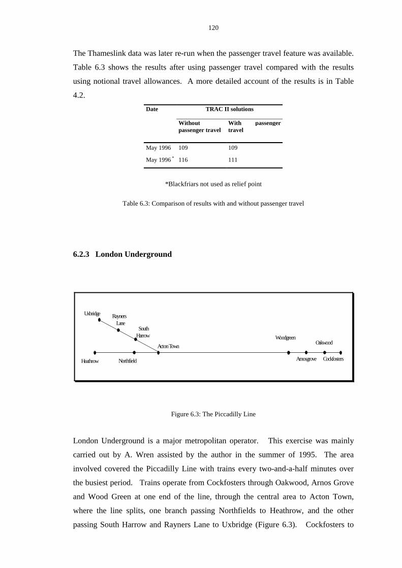
120
The Thameslink data was later re-run when the passenger travel feature was available.
Table 6.3 shows the results after using passenger travel compared with the results
using notional travel allowances. A more detailed account of the results is in Table
4.2.
TRAC II sol utionsDate
Wit houtpassenger travel
Wit h passengertravel
May 1996 109 109
May 1996 * 116 111
*Blackfriars not used as relief point
Table 6.3: Comparison of results with and without passenger travel
6.2.3 London Underground
Acton Town
SouthHarrow
RaynersLane
Uxbridge
NorthfieldHeathrow
Woodgreen
Arnosgrove
Oakwood
Cockfosters
Figure 6.3: The Piccadilly Line
London Underground is a major metropolitan operator. This exercise was mainly
carried out by A. Wren assisted by the author in the summer of 1995. The area
involved covered the Piccadilly Line with trains every two-and-a-half minutes over
the busiest period. Trains operate from Cockfosters through Oakwood, Arnos Grove
and Wood Green at one end of the line, through the central area to Acton Town,
where the line splits, one branch passing Northfields to Heathrow, and the other
passing South Harrow and Rayners Lane to Uxbridge (Figure 6.3). Cockfosters to
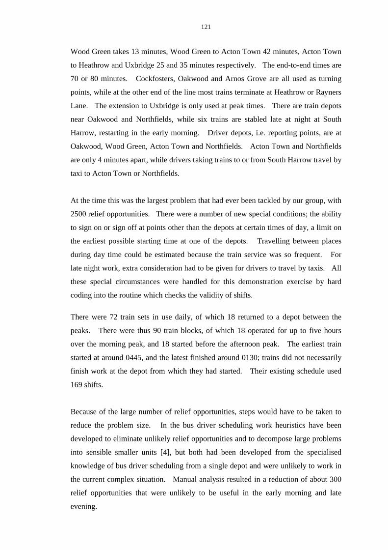
121
Wood Green takes 13 minutes, Wood Green to Acton Town 42 minutes, Acton Town
to Heathrow and Uxbridge 25 and 35 minutes respectively. The end-to-end times are
70 or 80 minutes. Cockfosters, Oakwood and Arnos Grove are all used as turning
points, while at the other end of the line most trains terminate at Heathrow or Rayners
Lane. The extension to Uxbridge is only used at peak times. There are train depots
near Oakwood and Northfields, while six trains are stabled late at night at South
Harrow, restarting in the early morning. Driver depots, i.e. reporting points, are at
Oakwood, Wood Green, Acton Town and Northfields. Acton Town and Northfields
are only 4 minutes apart, while drivers taking trains to or from South Harrow travel by
taxi to Acton Town or Northfields.
At the time this was the largest problem that had ever been tackled by our group, with
2500 relief opportunities. There were a number of new special conditions; the ability
to sign on or sign off at points other than the depots at certain times of day, a limit on
the earliest possible starting time at one of the depots. Travelling between places
during day time could be estimated because the train service was so frequent. For
late night work, extra consideration had to be given for drivers to travel by taxis. All
these special circumstances were handled for this demonstration exercise by hard
coding into the routine which checks the validity of shifts.
There were 72 train sets in use daily, of which 18 returned to a depot between the
peaks. There were thus 90 train blocks, of which 18 operated for up to five hours
over the morning peak, and 18 started before the afternoon peak. The earliest train
started at around 0445, and the latest finished around 0130; trains did not necessarily
finish work at the depot from which they had started. Their existing schedule used
169 shifts.
Because of the large number of relief opportunities, steps would have to be taken to
reduce the problem size. In the bus driver scheduling work heuristics have been
developed to eliminate unlikely relief opportunities and to decompose large problems
into sensible smaller units [4], but both had been developed from the specialised
knowledge of bus driver scheduling from a single depot and were unlikely to work in
the current complex situation. Manual analysis resulted in a reduction of about 300
relief opportunities that were unlikely to be useful in the early morning and late
evening.
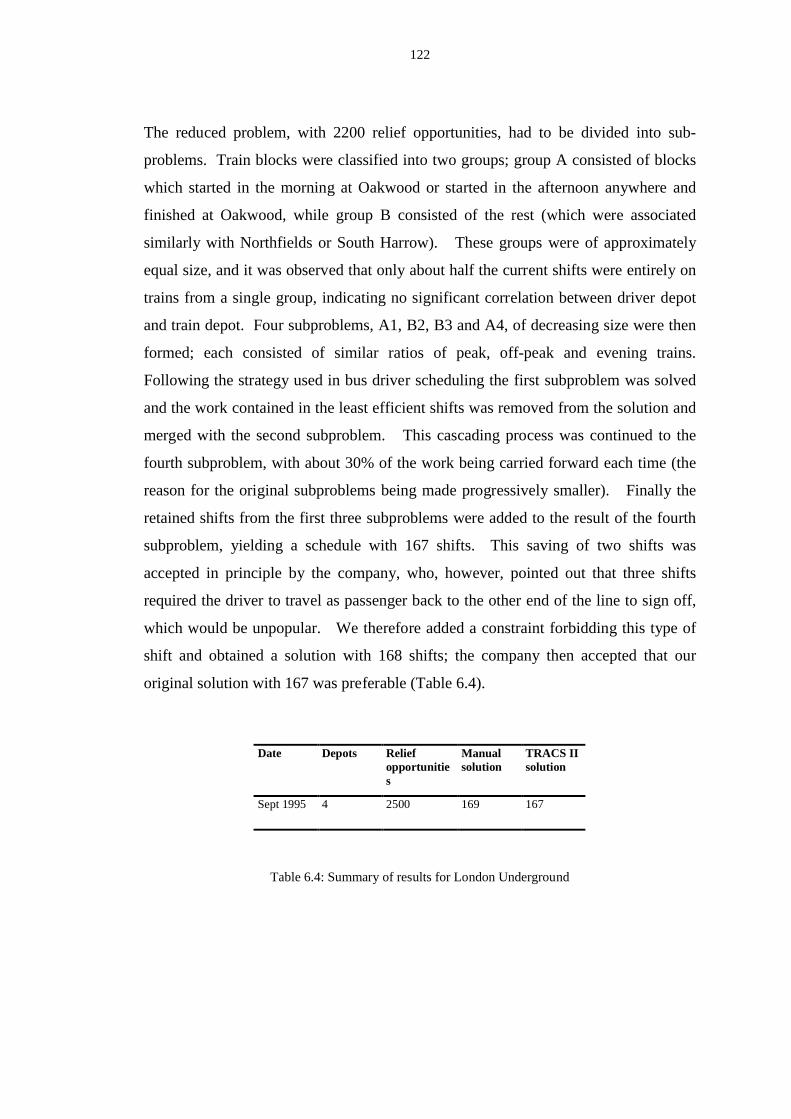
122
The reduced problem, with 2200 relief opportunities, had to be divided into sub-
problems. Train blocks were classified into two groups; group A consisted of blocks
which started in the morning at Oakwood or started in the afternoon anywhere and
finished at Oakwood, while group B consisted of the rest (which were associated
similarly with Northfields or South Harrow). These groups were of approximately
equal size, and it was observed that only about half the current shifts were entirely on
trains from a single group, indicating no significant correlation between driver depot
and train depot. Four subproblems, A1, B2, B3 and A4, of decreasing size were then
formed; each consisted of similar ratios of peak, off-peak and evening trains.
Following the strategy used in bus driver scheduling the first subproblem was solved
and the work contained in the least efficient shifts was removed from the solution and
merged with the second subproblem. This cascading process was continued to the
fourth subproblem, with about 30% of the work being carried forward each time (the
reason for the original subproblems being made progressively smaller). Finally the
retained shifts from the first three subproblems were added to the result of the fourth
subproblem, yielding a schedule with 167 shifts. This saving of two shifts was
accepted in principle by the company, who, however, pointed out that three shifts
required the driver to travel as passenger back to the other end of the line to sign off,
which would be unpopular. We therefore added a constraint forbidding this type of
shift and obtained a solution with 168 shifts; the company then accepted that our
original solution with 167 was preferable (Table 6.4).
Date Depots Reliefopportu nities
Manualsolution
TRACS IIsolution
Sept 1995 4 2500 169 167
Table 6.4: Summary of results for London Underground
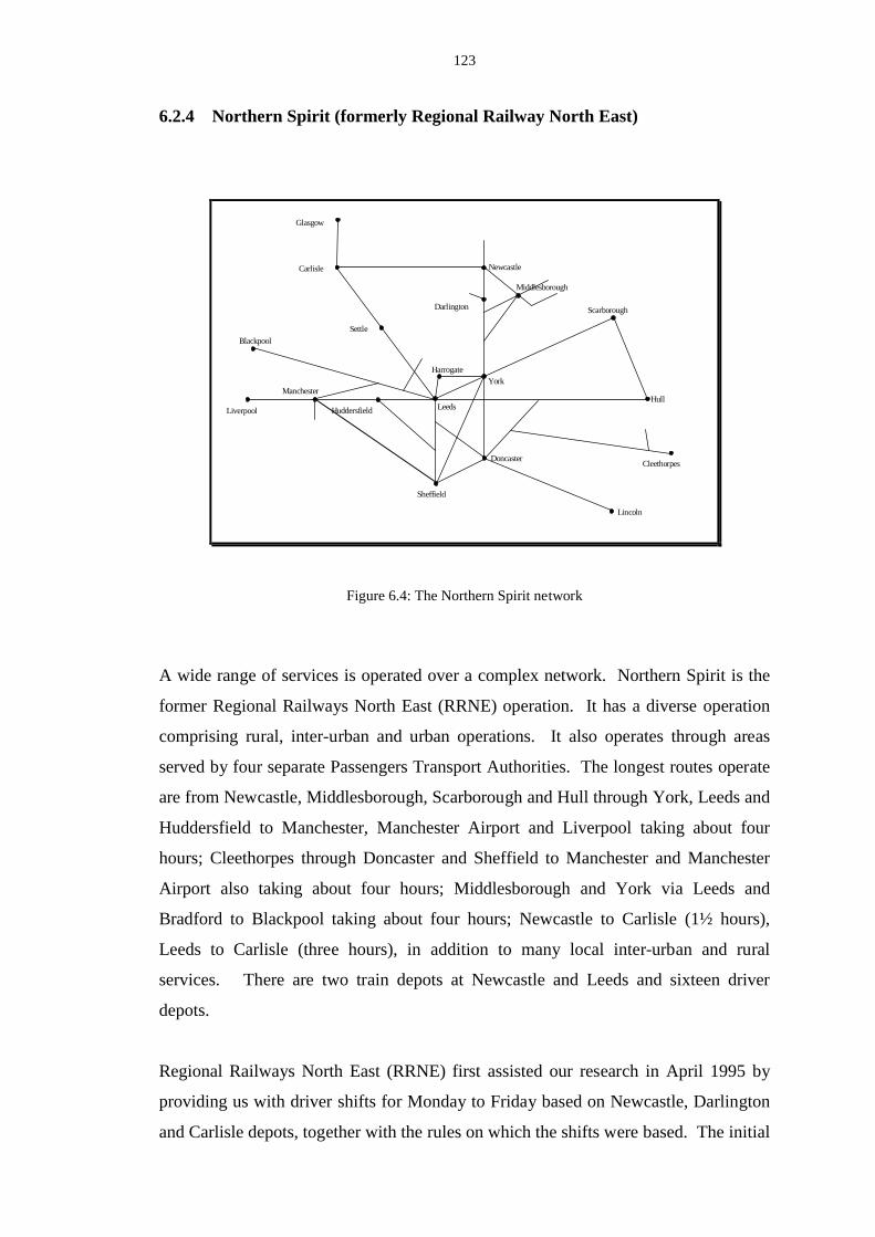
123
6.2.4 Northern Spirit (for merly Regional Railway North East)
Carlisle
Glasgow
Newcastle
Darl ington
Middlesborough
YorkHarrogate
Leeds
Manchester
Blackpool
Liverpool
Scarborough
Hull
Cleethorpes
Sheffield
Huddersfield
Doncaster
Lincoln
Settle
Figure 6.4: The Northern Spirit network
A wide range of services is operated over a complex network. Northern Spirit is the
former Regional Railways North East (RRNE) operation. It has a diverse operation
comprising rural, inter-urban and urban operations. It also operates through areas
served by four separate Passengers Transport Authorities. The longest routes operate
are from Newcastle, Middlesborough, Scarborough and Hull through York, Leeds and
Huddersfield to Manchester, Manchester Airport and Liverpool taking about four
hours; Cleethorpes through Doncaster and Sheffield to Manchester and Manchester
Airport also taking about four hours; Middlesborough and York via Leeds and
Bradford to Blackpool taking about four hours; Newcastle to Carlisle (1½ hours),
Leeds to Carlisle (three hours), in addition to many local inter-urban and rural
services. There are two train depots at Newcastle and Leeds and sixteen driver
depots.
Regional Railways North East (RRNE) first assisted our research in April 1995 by
providing us with driver shifts for Monday to Friday based on Newcastle, Darlington
and Carlisle depots, together with the rules on which the shifts were based. The initial
124
study combined an urban commuting area with a rural area and there were more
opportunities to relieve drivers compared to those for GNER but not as many as for
London Underground. Relief points were close together both in time and distance.
However an extra constraint placed upon the scheduling process was that not all the
drivers could drive on all parts of the network. Certain assumptions had to be made
about times allowed to travel as passenger between points on the system, as TRACS
II could not at that stage deal with passenger travelling. Also the feature of forming
shifts of more than three spells was not available at that time. Despite these
limitations, the schedules produced were satisfactory after minor adjustments, and
actually used four fewer shifts than the existing operation.
RRNE approached us in October 1995, asking our Group to repeat the exercise that
we had already carried out, but using a range of different operating scenarios. This
work was undertaken in the period up to March 1996, and assisted the company to
narrow the choice of scenario to a single set of rules affecting such matters as signing
on and off, preparation and disposal allowances and meal breaks, with three options
for other rules.
By the spring of 1996, TRACS II had been extended to allow the formation of shifts
involving more than three spells, and to incorporate provision for passenger travel on
trains of any appropriate company or indeed by taxis, provided that these had all been
included in the data. The following work was undertaken based on this new version.
In April, 1996 the SACM Group were commissioned by RRNE to apply alternative
scenarios to their whole Monday to Friday operation. This was by far the largest and
most complicated problem that had ever been tackled, with around twenty depots or
groups of drivers, and over 400 daily driver shifts. There were restrictions on route
and traction knowledge for each depot, so that any individual portion of train work
between relief opportunities could only be driven from a small number of depots.
The route knowledge of neighbouring depots did however overlap considerably, so
that the whole operation was a single interacting process rather than a set of individual
depot-based problems. The numbers of shifts to be assigned to certain depots were
also limited.

125
Ideally, if more time had had been given in this exercise, a solution strategy based on
subdividing a large problem as in the London Underground exercise should have been
developed. However, RRNE required us to obtain schedules as quickly as possible, it
was not possible to implement the strategy used in London Underground on carrying
work over between sub-problems. The problem was then subdivided into five
subproblems based on suitable combinations of depots, route and traction knowledge.
These subproblems were then solved in parallel and independently. For each
subproblem many tens of thousands of possible shifts were generated according to the
most restrictive of the possible scenarios. The shift generation program provides
information on any train work which cannot be covered according to the rules being
followed. This work was examined carefully, and dealt with by a number of actions.
Sometimes work was uncovered due to data errors or to inconsistencies in allocation
of work to subproblems. In other cases, work which was in theory suitable for one
subproblem could not be fitted together with other work in that subproblem to make
an efficient shift according to the parameters being followed. Our next task was
therefore to correct the errors and to exchange problematic work between
subproblems.
However, in some cases the problems had arisen because of real difficulties at certain
points. For example, to prevent the generation of too many shifts, TRACS II imposes
maximum lengths on the amount of idle time between components of a shift. At
certain places it was not possible to find matches for some incoming trains according
to these rules. We therefore had to allow the rules to be bent in certain
circumstances. In other cases, examination of the problem situation revealed that
there was no way of covering certain work according to the given operating scenario,
and some of the parameters originally stipulated had to be altered by agreement with
RRNE.
The first sets of shifts covering two scenarios were sent to RRNE about six weeks
after the start of the exercise. Following examination by RRNE some errors in the
data were corrected. There was also a new requirement for the system to allow for a
specified leeway whenever a driver has to change train either to carry on their duty or
to travel as passenger. This leeway feature was used as a safety measure for possible
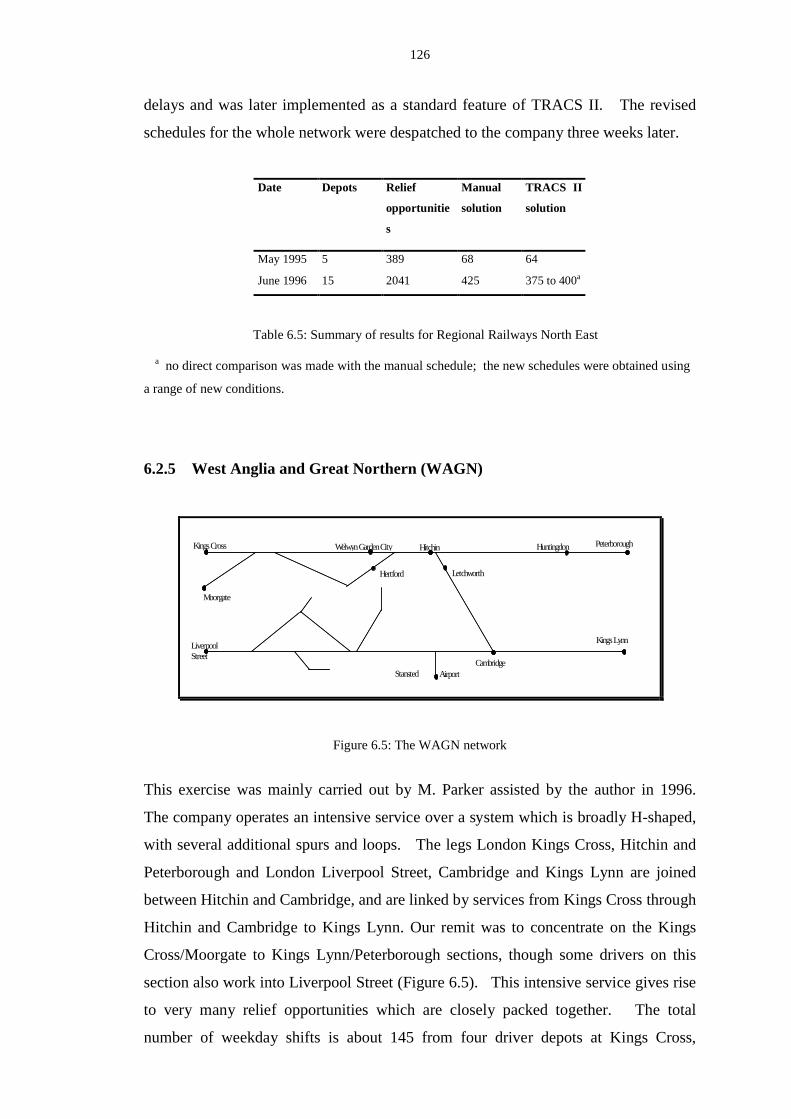
126
delays and was later implemented as a standard feature of TRACS II . The revised
schedules for the whole network were despatched to the company three weeks later.
Date Depots Relief
opportu nitie
s
Manual
solution
TRACS II
solution
May 1995 5 389 68 64
June 1996 15 2041 425 375 to 400a
Table 6.5: Summary of results for Regional Railways North East
a no direct comparison was made with the manual schedule; the new schedules were obtained using
a range of new conditions.
6.2.5 West Anglia and Great Northern (W AGN)
Peterborough
Kings Lynn
Hitchin
CambridgeStansted Airport
Hertford
Kings Cross
Moorgate
LiverpoolStreet
Welwyn Garden City
Letchworth
Huntingdon
Figure 6.5: The WAGN network
This exercise was mainly carried out by M. Parker assisted by the author in 1996.
The company operates an intensive service over a system which is broadly H-shaped,
with several additional spurs and loops. The legs London Kings Cross, Hitchin and
Peterborough and London Liverpool Street, Cambridge and Kings Lynn are joined
between Hitchin and Cambridge, and are linked by services from Kings Cross through
Hitchin and Cambridge to Kings Lynn. Our remit was to concentrate on the Kings
Cross/Moorgate to Kings Lynn/Peterborough sections, though some drivers on this
section also work into Liverpool Street (Figure 6.5). This intensive service gives rise
to very many relief opportunities which are closely packed together. The total
number of weekday shifts is about 145 from four driver depots at Kings Cross,
127
Hitchin, Peterborough and Kings Lynn. The journey times between Kings Cross and
Peterborough, Cambridge, and Kings Lynn are about 90 minutes, 70 minutes and 100
minutes respectively. The journey times between London Moorgate and Welwyn
Garden City and Hertford are about 45 minutes each. There is a combination of nine
express and stopping trains each hour resulting in three trains for Cambridge, one
train for Peterborough, one train for Huntingdon, and one train for Kings Lynn on the
Kings Cross to Kings Lynn and Peterborough sections, and from Moorgate, two trains
to Welwyn Garden City and one to Hertford. Peterborough drivers do not have route
knowledge from Hitchin to Cambridge and Kings Lynn, and Cambridge and Kings
Lynn drivers do not have the route knowledge from Hitchin to Peterborough.
The train work was presented in two parts: that covering work from Kings Cross and
Moorgate to Welwyn Garden City, Letchworth and Hertford and that covering Kings
Cross to Peterborough and Kings Lynn. The traction types were different for each
part. It was observed that there were few drivers who drove trains from both parts
and this seemed a reasonable way to subdivide the problem. Although dividing the
train work in this way would lose some of the flexibilit y afforded by a computerised
approach, it was felt to be worth pursuing. Two traction types are used but there are
no traction type restrictions. The first subproblem was solved and the work of the
least efficient shifts was carried forward to the second subproblem. This resulted in a
schedule with 141 drivers, four fewer than actually used.
One main feature of the manual schedule is the extensive use of passenger travelling.
A few of the passenger journeys involved travelling on three different trains together
with a walk. Currently, TRACS II only searches for passenger links involving a
maximum of two different vehicles plus further walking to or from points. Hence,
some of the passenger journey times have to be adjusted manually.
Another feature was that it was preferable for shifts to sign on and off outside the
‘unsocial hours’ period of 0000 - 0459 inclusive, otherwise penalty payments would
be incurred. The results of this exercise are summarised in Table 6.6.
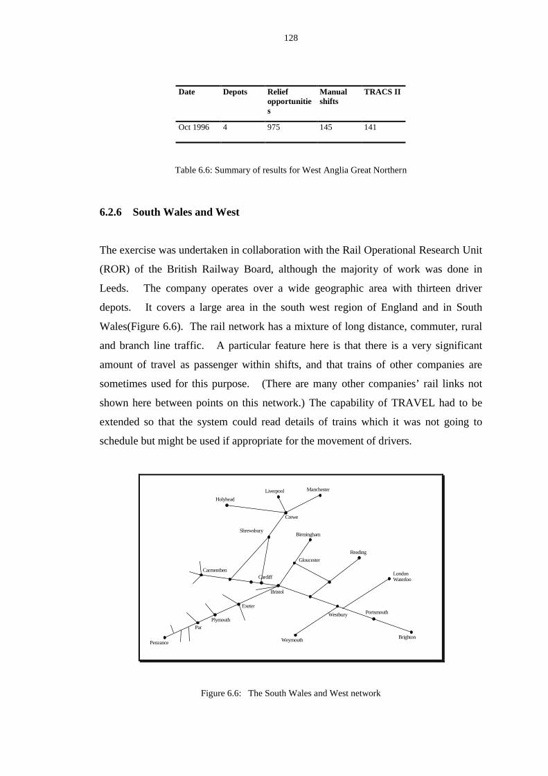
128
Date Depots Reliefopportu nities
Manualshifts
TRACS II
Oct 1996 4 975 145 141
Table 6.6: Summary of results for West Anglia Great Northern
6.2.6 South Wales and West
The exercise was undertaken in collaboration with the Rail Operational Research Unit
(ROR) of the British Railway Board, although the majority of work was done in
Leeds. The company operates over a wide geographic area with thirteen driver
depots. It covers a large area in the south west region of England and in South
Wales(Figure 6.6). The rail network has a mixture of long distance, commuter, rural
and branch line traffic. A particular feature here is that there is a very significant
amount of travel as passenger within shifts, and that trains of other companies are
sometimes used for this purpose. (There are many other companies’ rail links not
shown here between points on this network.) The capability of TRAVEL had to be
extended so that the system could read details of trains which it was not going to
schedule but might be used if appropriate for the movement of drivers.
Carmenthen
Bristol
Cardiff
Exeter
Westbury
Weymouth
Portsmouth
Brighton
LondonWaterloo
Reading
Birmingham
Gloucester
Shrewsbury
Crewe
Holyhead
Liverpool Manchester
Plymouth
Par
Penzance
Figure 6.6: The South Wales and West network
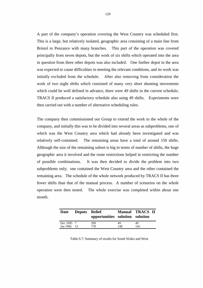
129
A part of the company’s operation covering the West Country was scheduled first.
This is a large, but relatively isolated, geographic area consisting of a main line from
Bristol to Penzance with many branches. This part of the operation was covered
principally from seven depots, but the work of six shifts which operated into the area
in question from three other depots was also included. One further depot in the area
was expected to cause difficulties in meeting the relevant conditions, and its work was
initiall y excluded from the schedule. After also removing from consideration the
work of two night shifts which consisted of many very short shunting movements
which could be well defined in advance, there were 49 shifts in the current schedule;
TRACS II produced a satisfactory schedule also using 49 shifts. Experiments were
then carried out with a number of alternative scheduling rules.
The company then commissioned our Group to extend the work to the whole of the
company, and initially this was to be divided into several areas as subproblems, one of
which was the West Country area which had already been investigated and was
relatively self-contained. The remaining areas have a total of around 150 shifts.
Although the size of the remaining subset is big in terms of number of shifts, the huge
geographic area it involved and the route restrictions helped in restricting the number
of possible combinations. It was then decided to divide the problem into two
subproblems only; one contained the West Country area and the other contained the
remaining area. The schedule of the whole network produced by TRACS II has three
fewer shifts than that of the manual process. A number of scenarios on the whole
operation were then tested. The whole exercise was completed within about one
month.
Date Depots Reliefopportunities
Manualsolution
TRACS IIsolution
Dec 1995 7 399 49 49Jan 1996 13 778 148 145
Table 6.7: Summary of results for South Wales and West
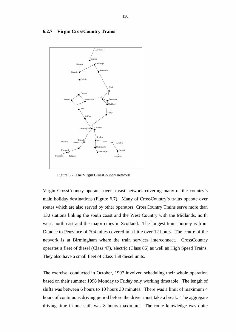
130
6.2.7 Virgin CrossCountry Trains
Figure 6.7: The Virgin CrossCountry network
Virgin CrossCountry operates over a vast network covering many of the country’s
main holiday destinations (Figure 6.7). Many of CrossCountry’s trains operate over
routes which are also served by other operators. CrossCountry Trains serve more than
130 stations linking the south coast and the West Country with the Midlands, north
west, north east and the major cities in Scotland. The longest train journey is from
Dundee to Penzance of 704 miles covered in a little over 12 hours. The centre of the
network is at Birmingham where the train services interconnect. CrossCountry
operates a fleet of diesel (Class 47), electric (Class 86) as well as High Speed Trains.
They also have a small fleet of Class 158 diesel units.
The exercise, conducted in October, 1997 involved scheduling their whole operation
based on their summer 1998 Monday to Friday only working timetable. The length of
shifts was between 6 hours to 10 hours 30 minutes. There was a limit of maximum 4
hours of continuous driving period before the driver must take a break. The aggregate
driving time in one shift was 8 hours maximum. The route knowledge was quite
Aberdeen
Dundee
Edinburgh
NewcastleCarstairs
Glasgow
Carlisle
Preston
Liverpool Manchester
Crew
York
LeedsDoncaster
Sheffield
Stafford
Derby
Birmingham Coventry
BristolSwansea
Penzance
Plymouth
Paignton
Reading
Basingstoke
Southampton
Brighton
London
Gatwick
131
complex especially around the Birmingham area. Traction knowledge was based on
four different types of locomotive. There were 11 driver depots spread all over the
country.
Originally, CrossCountry indicated that only crew depots and a few more points were
used for relieving crew. However, we identified 54 relief points in existing schedules
and it turned out to be a bigger exercise than was first anticipated.
At the early stage of the exercise, there had been problems in covering all the train
work. This was caused by some possible passenger travel trips not being available in
the data. This was solved by identifying these passenger trips and further possibilities
for driver travel to and from relevant points. Another issue was that the exercise was
based on a future (at that time) timetable when there was no manual schedule
available for comparison. Therefore there were difficulties in determining possible
relief points and drivers’ travel patterns. Also, the drivers travel on trains run by other
train operating companies as well as their own. Given the vast network of the
problem, it would be impossible for us to determine all the possible passenger
travelling trips for the driver without the detailed knowledge of the company’s
system. Theoretically, in order to find all the possible passenger travel times, we
would have to input most of the train times from the Great Britain Timetable into the
system and this was clearly impracticable. However, some passenger travelling
possibilities using the East Coast and West Coast timetables were manually input to
the system. Computationally, there were some occasions that the branch and bound
process of the ILP failed to get an integer solution.
Despite the above difficulties, a schedule of 153 shifts was produced. The company
then indicated that the average shift length of 9 hours 10 minutes was too high. A re-
run was therefore performed in order to bring the average shift length down to 8 hours
30 minutes. This was achieved by running the ILP a number of times and each time
with a different target number of shifts. The schedule which had the target average
and the lowest cost was chosen and this contained 162 shifts. Schedules with higher
numbers of shifts did not produce any improvement in average shift length, merely a
higher total cost. This was probably owing to the fact that the system was not making
use of all the feasible travelling arrangements because not all of this information was
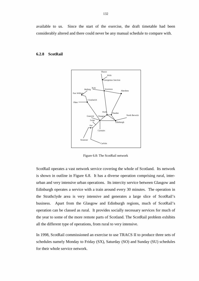
132
available to us. Since the start of the exercise, the draft timetable had been
considerably altered and there could never be any manual schedule to compare with.
6.2.8 ScotRail
Kyle
Thurso
Wick
Georgemas Junction
Mallaig
Fort Wil liam
CrianlarichOban
Aberdeen
DundeeNorth Berwick
Edinburgh
Glasgow
Perth
Carstairs
Gourock
Largs
Ayr
Carli sle
Stranraer
Inverness
Figure 6.8: The ScotRail network
ScotRail operates a vast network service covering the whole of Scotland. Its network
is shown in outline in Figure 6.8. It has a diverse operation comprising rural, inter-
urban and very intensive urban operations. Its intercity service between Glasgow and
Edinburgh operates a service with a train around every 30 minutes. The operation in
the Strathclyde area is very intensive and generates a large slice of ScotRail’s
business. Apart from the Glasgow and Edinburgh regions, much of ScotRail’s
operation can be classed as rural. It provides socially necessary services for much of
the year to some of the more remote parts of Scotland. The ScotRail problem exhibits
all the different type of operations, from rural to very intensive.
In 1998, ScotRail commissioned an exercise to use TRACS II to produce three sets of
schedules namely Monday to Friday (SX), Saturday (SO) and Sunday (SU) schedules
for their whole service network.
133
The data was based on the winter timetable of 1998. There were 19 driver depots
throughout Scotland. The scheduling conditions of ScotRail are very similar to other
train operating companies. Shift lengths can vary from 6 hours to 10 hours. There is
a limit of 4 hours 30 minutes on continuous driving constraint. Any turn round time
which is less than 10 minutes is counted towards the continuous driving. There can
be up to three mealbreaks in a shift. The lengths of mealbreak vary depending on the
shift length. For shifts whose spreadover was longer than 9 hours and with three
mealbreaks, their mealbreak lengths can be of different lengths, e.g. two 15 minutes
mealbreaks plus one 30 minutes mealbreak. This causes a problem to BUILD which
does not cater for different mealbreak lengths in a shift. However, after inspecting
ScotRail’s existing schedule, only four shifts out of the about 400 shifts have three
mealbreaks and most of these four shifts violated the precise combinations of break
lengths permitted according to the conditions specified to us. Because of lack of
resource, it was decided that no special arrangement for different mealbreak lengths
was to be implemented in this exercise.
The SX data is biggest amongst the three sets and is the first one to be tackled. There
are over three thousand relief opportunities and 25 traction types. The data is divided
into four sub-problems based on different regions:
1. South and West region of Glasgow;
2. North and East of Edinburgh;
3. Glasgow North Clyde;
4. Central, West Highland and Stirling
After results were produced from TRACS II , some re-grouping of work between the
sub-problems was needed in order to achieve the same distribution of shifts amongst
the depots as in the manual schedule. For example, the TRACS II results produced a
total of 29 shifts assigned to Perth depot whereas the manual schedule had 26 shifts at
Perth and there were 36 Glasgow Queen Street shifts in the TRACS II solutions
compared to 47 in the manual schedules. Hence work originally falling in the North
and East of Edinburgh (sub-problem 1) had to be re-assigned to the Central sub-
problem (sub-problem 4). There were some other similar re-distribution of work in
the other depots.

134
There were many problems encountered in this exercise. Many of them were
attributed to data errors. In addition, there were some computational difficulties. The
ILP process had difficulties in finding any solution for the North Clyde SO data.
Several ILP runs were tried with different target number of shifts but each time there
was no solution found in the branch and bound process. This was eventually solved
by running the BUILD process several times using different parameters in the labour
agreement file. The Edinburgh data demonstrates very similar difficulties.
The project started in late October, 1998, and after overcoming many problems, the
first satisfactory SX schedule was finalised in late November. Work was started
immediately on the SO data followed by the SU data. The SO schedule was produced
in December and the SU schedule was produced in early January, 1999. Table 6.8
shows the results of the exercise compared with the manual schedule.
Date Problems Depots Reliefopportunities
Manualsolution
TRACSIIsolution
Savings%
Nov 1998 SX 19 3445 365 350 4.1Dec 1998 SO 19 3079 334 314 6.0Jan 1999 SU 19 1264 156 141 9.6
Table 6.8: Summary of results for ScotRail
6.2.9 Other rail exercises
During this research, the SACM group has collaborated with three organisations to
exploit TRACS II commercially, two of which directly conducted scheduling
exercises using TRACS II on behalf of a number of operating companies. These
exercises are:
InterCity West Coast (on catering staff)
Mersey Rail
North London Railways
GNER
Great Western

135
Cardiff Valleys
Heathrow Express
English, Welsh and Scottish Railway
In these exercises, our commercial partners were responsible mainly for liaising with
the clients and to undertake the computer scheduling runs. We were responsible for
enhancing TRACS II whenever it was necessary to overcome any difficult y arising
during these exercises. In the case of the larger exercises like ScotRail and South
Wales and West most of the scheduling work was undertaken by our group.
6.3 Application of TRACS II in the bus situation
In Section 1.6, a comparison between the bus driver scheduling problem and the train
driver scheduling problem is made. It is concluded that the bus problem can be
considered as a special case of train driver scheduling. Hence TRACS II has been
used to solve bus problems and this section describes some of the exercises carried
out by our group.
6.3.1 Reading Buses
Wren and Kwan [76] report the installation of a bus and driver scheduling system of
which TRACS II is the driver scheduling component. This was the first commercial
implementation of TRACS II for a bus company.
By the middle of 1997, Reading Buses was running a total of 215 vehicles in seven
main scheduled groups. There were about 375 drivers employed with around 270
shifts on rotating rotas on a normal weekday. At that time, the company was planning
to relocate their existing driver depot, which was due to be redeveloped as part of a
shopping complex, to a new depot which was elsewhere in the town. The move was
planned to take place in February 1998. Since the new depot was less suitably placed
compared with the centrally located old depot, such a move was expected to lead to
higher operating costs, with most driver reliefs taking place at the station, or when
136
buses returned to the depot. The company forecast that such a move would result in
about 15 minutes less productive time per shift, or an increase of about 255 hours
weekly. This was based on the assumption that the resulting shifts were all legal. The
objective of the company to purchase a new driver scheduling system was to facilitate
the construction of schedules for the new depot as well as to investigate the likely
impact on schedules under alternative forms of labour agreement.
Although TRACS II had already had an extensive parameter list which could cater for
most of the operating conditions of any rail and bus organisation, there were some
conditions that are specific to Reading Buses that had to be catered for. Reading
Buses did not have a uniform maximum driving time a driver could be on duty
without a break. This maximum time varied according to the principal route being
followed by the bus. The company did not have any route knowledge similar to the
train situation. However, they had a ‘route diversity’ restriction. Bus routes are
grouped into different groups called ‘f amily route groups’. ‘Route diversity
restriction’ means that the first part of a shift before the mealbreak must belong to a
different family route group from the second part of the shift. In the situation where a
shift contains three or four spells, the route groups of each spell must be different
from the others. Split shifts were required in the Reading schedules. Unlike other
shifts, the mealbreaks of split shifts were not paid. Drivers of split shifts are paid for
a signing off allowance before the long mealbreak and a signing on allowance after
the mealbreak. These special requirements were incorporated into the system for the
company.
A computer schedule was produced for the old depot which strictly followed all the
conditions. The schedule used 136 shifts at a cost of 67786 minutes of paid time,
compared to 141 shifts and 69714 minutes in the manual schedule. This saving in
number of shifts and cost was judged sufficient on its own to justify the system costs.
Schedules were subsequently produced for the new Reading depot on 12 data sets,
namely urban and rural big bus and midi-bus for each of weekday, Saturday and
Sunday. All the data sets contain only one depot. The total weekly cost of the
schedules produced by TRACS II based on the new depot was 8479 hours compared
with 8366 hours for the manual schedules based on the old depot with 113 hours
increase. However, it was originally estimated that the increase would be about 255

137
hours by the company, TRACS II managed to lessen the increase in cost by more than
half. The saving was estimated by the company to be approximately £135,000 per
annum.
6.3.2 First Eastern Counties
In the spring of 1999, First Bus (the bus side of FirstGroup) set a test exercise to
potential suppliers of a scheduling system. This was based on four possible scenarios
derived from the Group’s Norwich operations. First Eastern Counties is one of 26
FirstGroup Bus subsidiaries providing bus services in East Anglia with depots in all
significant towns. The data of this exercise is based on the Monday to Friday bus
network provided within the city of Norwich in 1998. The network consists of six
main route groups which can be further sub-divided into 14 route variants. The
network of service is operated by three different types of vehicles, namely, Super Low
Floor Buses (SLF), Scania Buses and Leyland Olympian Buses. The last two types
are generally referred to as ‘Conventional Buses’.
There are three depots located outside Central Norwich: Roundtree Way, Vulcan
Road and Woodcock Road which is a sub-depot of Vulcan Road. All vehicles
returning to Woodcock Road at the end of service run via Vulcan Road depot to be
refuelled and cleaned. Drivers signing on at these three depots must also sign off at
the same depot. A bus station at Surrey Street in Central Norwich is also being used
as a driver signing on and off point. Hence there are effectively four driver depots.
Shifts are classified into two types: ‘five day week’ shifts which have a maximum
length of 8 hours 30 minutes; ‘four day week’ shifts whose length are between 9
hours 45 minutes and 12 hours 59 minutes.
The exercise involved producing schedules according to four different scenarios and
each of these scenarios was treated as an independent problem. Scenario one aims to
replicate their present operating conditions and the schedule produced would provide
a comparison with the current manual schedule; scenarios two, three and four are to
evaluate the cost implications of potential changes to the operating agreements.
138
Scenario one:
Scenario one allows both types of shifts to be present in the schedules. However, in
order to replicate their present conditions, the distribution of 4 day week and 5 day
week shifts per depot as in their existing schedules are to be followed. Also, drivers
of each depot are only allowed to drive a certain type of vehicle. One of the
scheduling conditions of scenario one is that there is a limit of ‘4 hours 8 minutes in
one period of driving, excluding starting and finishing allowance’. ‘One period’ of
driving means that only ‘wheel turning’ time is counted towards the 4:08 maximum.
Joinup time, travel time and signing on/off is not counted as worked time.
Another feature of this scenario is that the length of the mealbreak in the 4 day week
shifts can be variable. For instance, shifts that are over 11 hours long can either have
two 40 minutes minimum mealbreak or two mealbreaks with a total of 80 minutes
minimum of which two mealbreaks must be at least 30 minutes long. Since a good
number of shifts in the manual schedule have variable mealbreak lengths, in order to
have a fair comparison, this feature has been implemented in the shift generation
process. Shifts are paid through for their entire duration.
Scenario two:
The bus work of this scenario (also in scenario three and four) is based solely on those
in scenario one with the exclusion of a small amount of work related to one vehicle
being garaged overnight at a location away from Norwich. One main difference from
scenario one is that there is no limitation placed on each depot as to which types of
shift are allowed. There are some restrictions on the types of vehicle a driver of a
particular depot can drive but to a lesser extent compared with scenario one. Another
difference is that the maximum length in one period of driving is extended to 5:30.
This is in accordance with the national law. One major difference is that ‘a period of
driving’ in this scenario (also in scenario three and four) means wheel turning time
plus joinup. Both 4 day week and 5 day week shifts are allowed in this scenario and
shifts are paid from sign on to sign off.
139
Scenario three:
Scenario three is based upon scenario two but there is a maximum work content of 9
hours in each shift and there is a desired average work content of less than 8 hours at
each location. One difference from the above two scenarios is that the drivers will be
able to sign on and off at either their home depot or at the Surrey Street Bus Station in
the city centre. Another difference is that there is no restriction on the type of vehicle
the driver of different depots can drive. The maximum length of a shift is 12 hours
and there is no distinction as to 4 day week and 5 day week type of shifts. Shifts are
paid for their entire duration except that the first two hours of their combined
mealbreak duration are unpaid.
Scenario four:
Scenario four is based upon scenario three but it restricts the maximum period of
driving before a break is needed to 4:30, after which a break of 45 minutes must be
taken. The break can be replaced by two breaks of which one must be at least 30
minutes and the other 15 minutes. The maximum length of a shift is 13 hours. Shifts
are paid from sign on to sign off except the first 45 minutes of the combined
mealbreak duration. These conditions are the requirement laid out in EC law.
The Norwich data is fairly complex because a lot of the features which are for train
driver scheduling are being used here. They are summarised as follows:
• There are four depots in this exercise and drivers must sign on and sign off at the
same depot (except in scenario three and four)
• Passenger travel is required for the drivers, after signing on at one of the depots, to
travel to a location in the city centre to start the first piece of work. Similarly,
passenger travel is needed for the driver to travel from city centre locations to sign
off at the home depot. However, passenger travel during joinup and mealbreaks is
not required as the locations are situated in the city centre and they are within
walking distance.
140
• There are different activities in addition to the driving work that have to be
allowed for in addition to driving. These activities, e.g. 5 minutes for re-fueling, 5
minutes to ‘cash in’, are similar to the non-driving work in the train situation.
These allowances have to be modelled as if they are the vehicle preparation,
disposal time as in the train situation.
• There is restriction on the type of vehicle which a driver of a particular depot can
drive. This is being modelled as traction knowledge in train problems.
There are many relief opportunities in the data (e.g. 887 in the base scenario) for a
problem of around 70 shifts. Also, in the first scenario, the maximum continuous
driving before a driver must take a break is 4 hours 8 minutes and the spreadover
allowed is a very wide range (up to 13 hours). As a result, there are a large number of
possible four spell shifts formed by the shift generation. Very tight parameters were
therefore used to restrict the number of potential shifts. Unfortunately, the shift
selection process failed to find any integer solution even although the target number
of shifts was raised ten times from 68 to 78 for the base scenario.
Eventually, the problem was solved by manually deselecting about half of the relief
opportunities. The problem size was therefore substantially reduced and TRACS II
was able to produce good solutions.
The only comparison that can be made against any existing schedule is Scenario One.
The schedule for the base scenario produced by TRACS II has 69 duties with a total
cost of 756.25, which is cheaper than the manual schedule which has 70 shifts costing
764:49.
In examining the existing manual schedule, there are a number of instances in which
the existing conditions of Scenario One are violated. Had the violation of the
conditions as in the existing schedule been allowed, TRACS II could probably have
been able to produce even more efficient schedules. Another observation of the
manual schedule is that there are a number of shifts with five spells of work. The
shifts that TRACS II produced have a maximum of four spells.
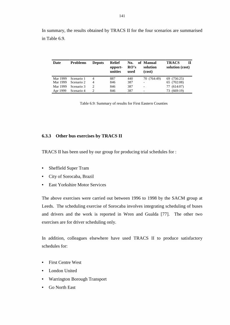
141
In summary, the results obtained by TRACS II for the four scenarios are summarised
in Table 6.9.
Date Problems Depots Reliefopport-unities
No. ofRO’sused
Manualsolution(cost)
TRACS IIsolution (cost)
Mar 1999 Scenario 1 4 887 440 70 (764:49) 69 (756:25)Mar 1999 Scenario 2 4 846 387 - 65 (702:08)Mar 1999 Scenario 3 2 846 387 - 77 (614:07)Apr 1999 Scenario 4 2 846 387 - 73 (669:19)
Table 6.9: Summary of results for First Eastern Counties
6.3.3 Other bus exercises by TRACS II
TRACS II has been used by our group for producing trial schedules for :
• Sheffield Super Tram
• City of Sorocaba, Brazil
• East Yorkshire Motor Services
The above exercises were carried out between 1996 to 1998 by the SACM group at
Leeds. The scheduling exercise of Sorocaba involves integrating scheduling of buses
and drivers and the work is reported in Wren and Gualda [77]. The other two
exercises are for driver scheduling only.
In addition, colleagues elsewhere have used TRACS II to produce satisfactory
schedules for:
• First Centre West
• London United
• Warrington Borough Transport
• Go North East
142
6.3.4 Conclusions
The exercises have been carried out over the years of this research and they provide
better insight into the train problem than before. During this time, a method of
constructing operable driver shifts has evolved from a very crude prototype to a
sophisticated process which can handle most of the operating conditions of the train
problems of the U.K. Table 6.10 summaries the results of these exercises and shows
how the software evolves over the duration of this research. It shows the dates of the
exercises, the size of the problems in terms of number of relief opportunities, the
manual solutions, the TRACS II solutions and the new features added to BUILD as
the system gradually evolved over the years. Through these exercises, we have
demonstrated that the two stage approach proposed in Chapter One is capable of
tackling the train problems and producing efficient train driver schedules according to
widely differing and complex circumstances. In almost all cases the schedules
produced have been acceptable to management and usually contain fewer shifts and
are cheaper than existing schedules. The system can be used to compile production
schedules as well as to investigate alternative operating scenarios, such as closing
down a depot, or adopting different working rules.
In the bus situation, the most complicated problem encountered is the First Eastern
Counties which is more complex than other bus problems we have encountered
before. Other bus problems described here are comparatively more straightforward.
The bus exercises have also demonstrated that TRACS II can solve bus driver
scheduling problems and can produce very good production schedules.
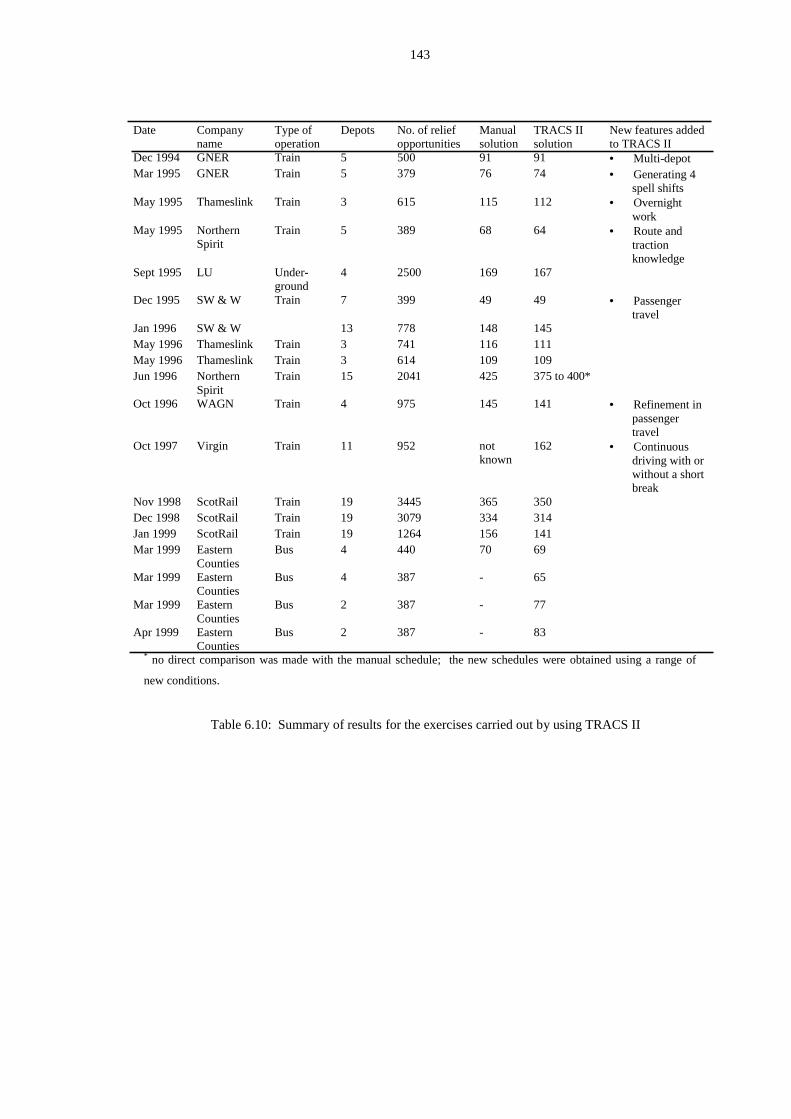
143
Date Companyname
Type ofoperation
Depots No. of reliefopportunities
Manualsolution
TRACS IIsolution
New features addedto TRACS II
Dec 1994 GNER Train 5 500 91 91 • Multi-depotMar 1995 GNER Train 5 379 76 74 • Generating 4
spell shiftsMay 1995 Thameslink Train 3 615 115 112 • Overnight
workMay 1995 Northern
SpiritTrain 5 389 68 64 • Route and
tractionknowledge
Sept 1995 LU Under-ground
4 2500 169 167
Dec 1995 SW & W Train 7 399 49 49 • Passengertravel
Jan 1996 SW & W 13 778 148 145May 1996 Thameslink Train 3 741 116 111May 1996 Thameslink Train 3 614 109 109Jun 1996 Northern
SpiritTrain 15 2041 425 375 to 400*
Oct 1996 WAGN Train 4 975 145 141 • Refinement inpassengertravel
Oct 1997 Virgin Train 11 952 notknown
162 • Continuousdriving with orwithout a shortbreak
Nov 1998 ScotRail Train 19 3445 365 350Dec 1998 ScotRail Train 19 3079 334 314Jan 1999 ScotRail Train 19 1264 156 141Mar 1999 Eastern
CountiesBus 4 440 70 69
Mar 1999 EasternCounties
Bus 4 387 - 65
Mar 1999 EasternCounties
Bus 2 387 - 77
Apr 1999 EasternCounties
Bus 2 387 - 83
* no direct comparison was made with the manual schedule; the new schedules were obtained using a range of
new conditions.
Table 6.10: Summary of results for the exercises carried out by using TRACS II
144
Chapter Seven
The ILP method for shift selection and its
computational difficulties
7.1 Introduction
This chapter gives an overview of the Integer Linear Programming (ILP) method used
for shift selection in TRACS II . Smith[2] and Wil lers[8] gave more detailed accounts
of the solution method. The ILP method used in TRACS II can produce a near
optimal solution in many cases but it also has its limitations. In addition to a
limitation in problem size that it can tackle, the process may sometimes fail to
produce any integer solution in the branch and bound process. The computational
difficulties of the ILP will be discussed in this chapter.
7.2 The Integer Linear Programming Model for shift selection
The shift selection stage of TRACS II involves solving a set covering model which
ensures that each piece of work is covered by at least one driver and the total cost is
minimised.
If there exist n different valid shift variables (xj) that could be used to cover a given
vehicle schedule and m work piece constraints, the problem may be formulated as
follows:

145
Minimise j
n
1jj xc∑
= (7.1)
subject to the constraints:
j
n
1jji xa∑
=
≥ 1, for i = 1, 2, ..., m (7.2)
where xj are 0-1 variables, for j = 1, 2,..., n ;
aij are constants whose values are either 0 or 1 ;
cj are positive constants reflecting the shift costs.
The variable xj represents whether a shift j is selected, and each constraint is
associated with a work piece to be covered; aij is 1 if shift j covers work piece i and is
0 otherwise. The cost of shift j is cj. This is a set covering problem in which every
work piece (i) must have at least one shift variable (j) assigned to it:
The objective function (7.1) is to minimise the overall cost of the solution. In TRACS
II the objective function takes into account a number of requirements to produce an
efficient driver schedule. The requirements are listed as follows:
• Minimising uncovered work pieces. If the process cannot remove all the
uncovered work pieces eventually, the process will be terminated.
• Minimising the number of shifts used in the schedule.
• Avoiding shifts which contain undesirable features.
• Minimising wage costs.
• Minimising the total amount of overcovered pieces of work.
The objective function of the ILP of TRACS II takes the form:
Minimise j
n
1jjxc∑
=
+ i
m
1ii ud∑
=
+ i
m
1iioe∑
= (7.3)
146
While the constraints take the form :
j
n
1jji xa∑
=
+ ui – oi = 1 for i = 1, 2, ..., m (7.4)
Plus any user-defined side constraints such as restricting the number of shifts
of some depots.
where ui is 1 if workpiece i is uncovered, 0 otherwise ;
oi is the number of times that workpiece i is overcovered ;
di is a large constant for reducing the number of uncovered pieces;
ei is a constant for reducing the amount of overcovered pieces;
cj is the cost of shift j, plus a large constant.
7.2.1 Solution strategy used in TRACS II
The solution strategy for the ILP method of TRACS II originated from the ILP
algorithms used in IMPACS. The ILP mathematical programming solver of IMPACS
is a package of Fortran subroutines called ZIP originally supplied by Ryan [73] in
1980. The user routines which tailor the package for use in driver scheduling have
been extensively modified over the years [2]. The solution strategy used in the ILP
algorithm in IMPACS comprises of two stages: the integer relaxation phase and the
branch and bound phase.
7.2.1.1Integer relaxation phase
Step 1
Shifts are ranked when they are constructed according to a simple formula which
measures their efficiency. All three and four spell shifts and shifts with a low ranking
are temporarily excluded. The integrality constraints on the shift variables are
relaxed so that fractional values are allowed. The relaxed model is solved over the
selected shifts using a primal steepest edge[78] variant of the Revised Simplex
Method with a starting initial solution formed by a heuristic.

147
Step 2
The shifts that were excluded before are restored and the LP relaxation is re-optimised
over the whole set of shifts, again, using the primal steepest edge algorithm until a
solution is found. The sum of the shift variables in the solution, T, will be used as the
target number of shifts in the final schedule. T will be rounded up to the next integer
if it is fractional.
Step 3
Penalty costs which are used to discourage shifts with some undesirable
characteristics, e.g. late night shifts, are added to the appropriate shifts in the whole
set. Two extra constraints are added:
i
m
1i
u∑=
≤ 0 (7.5)
j
n
1j
x∑=
≤ T (7.6)
(7.5) disallows uncovered pieces and (7.6) ensures that subsequent re-optimisation
will not result in a solution which exceeds T. The new model is re-optimised using
the primal steepest edge algorithm. The new re-optimisation process is to minimise a
cost function, incorporating penalty costs, with the above added constraints that the
total number of shifts does not exceed the number found in Step 2. The revised
objective function is as follows:
Minimise jj2
n
1jj1 x)cc( +∑
=
+ i
m
1ii ud∑
=
+ i
m
1iioe∑
= (7.7)
where c1j includes the shift costs and a large constant for minimising shifts
c2j is the penalty cost for discouraging unpopular features in shifts.
Step 4
If the sum of the shift variables in the solution found is non-integral, integrality will
be imposed on the total number of shifts as an extra constraint. The new model is re-
optimised using a Dual Simplex algorithm.

148
Step 5
If the solution is integral, the process stops. Otherwise, a branch-and-bound process
will follow.
7.2.1.2Branch and bound phase
The branch and bound process is based on the non-integer relaxed LP solution found
above and consists of the following steps:
Step 1
Reduce the size of the shift set entering the branch and bound phase by a technique
called Reduce which will be discussed in Section 7.2.1.3.
Step 2
Using the current relaxed LP solution, for each relief opportunity within any non-
overcovered workpieces, calculate the sum of the xj variables which have work pieces
starting at this relief opportunity. Select a relief opportunity that has a fractional
value. Based on this relief opportunity, create a node with two branches, one
requiring the selected relief opportunity not to be used and the other requiring that
relief opportunity to be used. This branching strategy is called Relief time Branching.
There are two other less frequently used branching strategies: Constraint Branching
and Variable Branching. Constraint branching, originally introduced by Ryan [73],
involves taking a pair of work pieces such that the sum of the shift variables which
cover both constraints is strictly fractional. Two branches are formed such that some
shift variables are banned on each branch: those covering both work pieces are
banned on the zero branch and those covering one piece but not the other are banned
on the one branch. Variable branching involves branching on a variable which has a
fractional values. If a relief time branch cannot be formed, TRACS II will try to form
a constraint branch and failing that, TRACS II will form a variable branch.
Step 3
If one of the stopping criteria (as explained below) is met, stop the process. The last
integer solution, if found, is the best integer solution.

149
Select a node having at least one unsolved branch and select one of this node’s
unsolved branches.
Step 4
Solve the selected branch using Dual Simplex algorithm. If the branch is fathomed,
return to Step 3. If a non-integer solution is found, return to Step 2, otherwise, an
integer solution is found, go to Step 5.
Step 5
Calculate a cut-off value of the integer solution. Any node having an objective value
greater than this cut-off value is not selected, and the solution of any branch is
discarded if its objective value is greater than this value. Go to Step 3.
Stopping criteria
1. No nodes can be selected.
2. The number of nodes created exceeds the maximum limi t imposed (500 at
present).
3. The number of nodes having one or more unsolved branches exceeds the
maximum limi t imposed (currently it is 400).
Generally, the branch and bound stage of finding an integer solution is usually the
most time-consuming and difficult. For practical reasons, the search for integer
solution in the search tree cannot be allowed to go on forever. Hence a limit on the
total number of nodes and how many of them are active at any one time has to be set
(as in Stopping criteria 2 and 3).
7.2.1.3‘Reduce’ heuristic
Wren and Smith [4] used this heuristic to reduce the number of variables to be
considered during the brand and bound search. It is based on the belief that there are
at least some good integer solutions which are similar to the relaxed solution.
150
Therefore the fractional shifts would give an indication of how the schedule might be
covered in an integer solution.
The reduction technique assumes that an acceptable integer solution can be found by
restricting the choice of relief opportunities to only those used by the set of shifts in
the relaxed solution, shifts using any other relief times are banned. The reduction
technique has the danger of banning shifts which might be crucial in forming the only
integer solutions with the required number of shifts, but usually there are many
different possible integer solutions with the required number of shifts and the
reduction technique is unlikely to exclude them all.
Willers [79] improved the reduction technique further by eliminating any unused
relief opportunities which in turn eliminated the workpiece constraints surrounding it.
The revised reduction technique is a standard feature of TRACS II which has been
successful in reducing the problem size and producing good integer solutions.
7.2.2 Recent improvements to the ILP method
The above solution strategy was implemented in the IMPACS system in the early
1980’s and was adopted in the original version of TRACS II . Two recent researches
into ways to improve the method and alternative strategies to the ILP were completed
at Leeds. They have been briefly mentioned in Chapter Five. These improved ILP
methods were implemented and incorporated into the TRACS II system for train
driver scheduling. The improved mathematical programming solver is called
SLPZIP. The improvements are briefly outlined in the following sections. Willers
[8] and Fores [9] describe these improvements in greater detail.
7.2.2.1Sherali weighted objective function
Willers[8] adopted the Sherali[80] weighted objective function approach. This
combines the objectives of minimising the number of shifts (Section 7.3) and the total
shift cost with any penalty cost added (Section 7.6), while maintaining their
preference ordering. Willers replaced these two objective functions by a single
151
weighted objective function known as Sherali weighted objective function. The new
relaxed LP model using this Sherali weighted objective function is then solved using a
primal steepest edge approach. Willers used a steepest edge Dual Simplex algorithm
for subsequent re-optimisation of the relaxed LP and the branch and bound process.
Willers used an improved ‘Reduce’ (Section 7.2.1.2) to enable many constraints to be
deleted immediately before the branch and bound process. The reduction in the
number of constraints leads to reduction in solution time of the branch and bound
phase.
On a sample of 20 bus driver scheduling problems, Willers reported the new model
produced an average reduction in execution time of approximately 50%.
7.2.2.2 A column generation approach
The mathematical process in ZIP requires all the shifts to be available for the LP
process. Fores [81, 82, 83] uses a column generation approach which only requires a
subset of the columns (shifts) to be available at the beginning. A revised simplex
method is used to find the solution which is optimal over the subset. Then new
columns with favourable reduced costs are added to the subset which is then re-
optimised over the new set. When no more columns which would improve the
objective can be added to the subset, the solution of the relaxed LP is the overall
optimal solution of the LP relaxation.
Fores implemented the column generation approach using the Sherali weighted
objective function into the TRACS II mathematical programming solver. This
method decreases the search space tremendously. The result of using this approach is
that many more shift variables are being considered and hence sometimes better
schedules can be produced with fewer shifts than before. Fores reported an
improvement in the number of shifts in 5 out of 7 of the test sets and an improvement
in execution time of 41%.
152
7.3 Computational diff iculties of the ILP method
The aforesaid improvement methods on the ILP process are centred on the
improvement of the processing time and the ability to input a larger set of potential
shifts. Although Willers has made some changes to the branch and bound method,
they are for improving the solution time only. The branching strategies used in the
branch and bound process are very similar to those used in ZIP.
7.3.1 Failure to find an integer solution in TRACS II
One inherent problem in the ILP approach is that the branch and bound algorithm
does not always find an integer solution. Referring to the stopping criteria in Section
7.2.1.2, two different situations can occur:
1. The search terminates because all nodes of the search tree have been fathomed.
2. The search terminates because one of the limits of the number of created nodes or
active nodes has been reached.
In the first situation, because of the side constraints operating during the branch and
bound process, e.g. the target number of shifts derived from the relaxed LP solution,
the solution is likely to need an extra shift. However, termination might also be due
to the reduction heuristic described in Section 7.2.1.3 which has excluded some vital
shifts before entering the branch and bound process.
In the second situation, there may be some integer solutions further down the branch
and bound tree and the search terminates before reaching it. This usually implies that
their objective values may be much higher than the relaxed optimum, and the node
selection strategy which is based on objective values makes them hard to find.
Situation 2 is the most common situation and accounts for over 90% of the situations
when TRACS II fails to find an integer solution. When no integer solution can be
found the course of action to be taken may involve one or a combination of the
following:

153
1. Re-iterate from the potential shift generation stage at the very beginning in order
to derive a different shift set for the ILP, e.g. by changing some control
parameters; or modifying the relief opportunities.
2. Reduce the size of the shift set input to the ILP by getting rid of shifts that are
considered to be less useful towards an integer solution than the others. Process
SIEVE (Section 5.8.1) in TRACS II can be used for reducing the size of the input
shift set.
3. Increase the target of total number of shifts, T, and re-run the ILP process only.
4. Impose side constraints, e.g. restriction on numbers of shifts of certain types, and
re-run the ILP. This has the effect of restricting the search space in branch and
bound.
Any of the above requires the ILP to be re-run. For some train driver scheduling
problems, there may be many iterations involved before an integer solution is found.
This can be extremely time-consuming.
7.3.2 Diff iculties arising in the multi-depot train problems
In bus driver scheduling problems, an integer solution has almost always been found
at the target level, T, ascertained in the revised relaxed solution of the integer
relaxation phase (Section 7.2.1.1). In the train situation, it is usually very difficult to
achieve T for which there might be an integer solution. When branch and bound fails
to find an integer solution, the normal course of action is to revise T and re-run the
ILP process. There is, again, no guarantee that an integer solution can be found with
the revised target. In some cases (some examples are described in Section 7.3.5), a lot
of time is wasted in runs which terminate inconclusively after the maximum number
of nodes (500) explored has been exceeded.
One difficult y identified is that there is no way to determine speedily whether it is
worth looking for a solution at a certain target. The diffi culty in ascertaining a target
arises, perhaps partly, from the fact that there is often more than one depot in the train

154
problems. In multi-depot problems, the minimum number of shifts suggested by the
revised relaxed solutions may contain non-integer values of shifts for each depot.
When integrality is imposed on the solution, it may be necessary for the shift totals of
these depots to be rounded up to the next nearest integer. As a result, the total number
of shifts increased is greater than one. For example, if the relaxed solution on a three-
depot problem is:
Depot 1 : 22.3 rounded up to 23 shifts
Depot 2 : 33.4 rounded up to 34 shifts
Depot 3 : 44.2 rounded up to 45 shifts
Total = 99.9 (non-integer) 102 (rounded up)
The target, T, imposed by the ILP on the above example is 100 whereas the solution
may require at least 102 shifts. However, even if a revised target exists which takes
into account of rounding each depot up separately from the relaxed solution, there is
usually difficult y in finding it and many experimental runs will be undertaken in
which 500 nodes are explored unsuccessfully. One possible explanation is that the
constraints imposed by route and traction knowledge have similar effects on the
relaxed solution as the depot constraints and make it even harder to determine the
target number of shift required.
7.3.3 Size of problems
Although the BUILD process can create a virtually unlimited number of potential
shifts, there is a limit on the size of the problem to be handled by the ILP process of
TRACS II . The current limit is 1,500 on the work piece and side constraints (m
rows). Although the ILP process can accept more than 100,000 shifts as input, the
column generation method only keeps up to a maximum of 30,000 shifts as sub-set in
memory. Whenever this maximum is reached, the column generation will halt the
ILP process. Although these limits can be extended, there will also be limits imposed
on the problem size that the ILP can handle.

155
These current limits are very adequate for bus driver scheduling problems and
medium-sized train problems. However, some of the train problems are very large
(e.g. Northern Spirit and ScotRail) and these problems have to be sub-divided. Sub-
dividing a problem may risk losing optimality. Research in the decomposition of
large problems have been focused on bus operations. There is yet no researched
method for decomposing train problems.
7.3.4 Robustness of the core routines in the ILP process
The core routines of the ZIP package are still in use in the TRACS II mathematical
programming solver. The core routines consist of a set of subroutines for handling
sparse linear programming bases which are part of the Harwell Subroutine Library;
these are described by Reid [84]. These routines, which were developed in the
1970’s, sometimes cause the ILP process to crash. The cause of the failure is usually
very difficult to trace because these routines are impossible to maintain. The usual
action is to perturb the input potential shift set to the ILP process by reducing the
number of shifts slightly or re-creating a new set.
7.3.5 Examples of the computational dif ficulties in case studies
There are a number of occasions when the ILP solver of TRACS II has difficulties in
finding integer solutions. The following are just two examples showing the
difficulties and how these are eventually resolved.
7.3.5.1First Eastern Counties
The Eastern counties exercise has four scenarios which are based on more or less the
same amount of vehicle work. The frequency of service is quite intensive and,
although the problem size is small in terms of working hours, there are 887 relief
opportunities in the problem. Because of the wide range of spreadovers allowed (up
to 13 hours), and because of the large number of possible four spell shifts, fairly tight
parameters were used for BUILD. In the base scenario, initiall y, there were around
156
100,000 shifts created by BUILD. The optimal solution suggested a target of 66 shifts
in the relaxed LP but the branch and bound process failed to find an integer solution.
Different target numbers of shifts were therefore used for ten ILP runs and each time
the branch and bound process failed to find any integer solution even when the target
was raised to 76. Subsequently, even the whole TRACS II process was re-run using
different parameters to create smaller sets of shifts and still no integer solution was
found. Eventually a substantial proportion of the relief opportunities (440 out of 887)
was de-selected to reduce the problem size. The relaxed solution for the base scenario
was 68 shifts and the integer solution had 70 shifts.
7.3.5.2ScotRail
In one of the sub-problems, North Clyde Saturday (Section 6.2.8), there was difficulty
in getting a solution from the ILP. There is a limit (currently 500) on the number of
nodes on the branch and bound tree to be explored, and often the limit is reached
before an integer solution can be found, if it exists. The mathematical process was
then re-iterated by forcing it to look for a solution with one more shift than the last
target. After raising the target ten times, there was still no solution produced. A
solution was eventually produced by re-creating a new set of shifts in a different way.
There was still no logical explanation as to why the original set of data failed to
produce any solution at all. When the data is erroneous the situation is even worse
because there is no way to predict what difficulties are caused by the errors.
7.4 Conclusions
The ILP methods used in shift selection have been briefly discussed together with
various techniques and enhancements made in recent years. The TRACS II system is
very capable of solving train driver scheduling problems. However, in some of the
real life problems encountered, much time has been wasted in the ILP process in order
to obtain an integer solution. In the train problems, it is often difficult to determine a
target number of shifts for which a solution can be found. The target suggested by the
revised relaxed LP solution often has to be raised whenever the branch and bound
process fails to get an integer solution for a particular target. Although recent

157
research work has resulted in faster mathematical programming algorithms and
allowed a larger input potential shift set, the chance of the branch and bound process
of finding an integer solution has not been improved.
Current research by colleagues is aimed at addressing the problems in the ILP
outlined in Section 7.2. However, since the branch and bound process is identified as
a potential bottleneck in the train driver scheduling process as a whole, one of the
goals of the current research is to explore the use of Genetic Algorithms in finding a
satisfactory integer solution much more quickly as an alternative to the branch and
bound process in the ILP.
158
Chapter Eight
A Genetic Algorith m framework for shift
selection
8.1 Introduction
This chapter discusses the use of a Genetic Algorithm (GA) for solving the set
covering problem as formulated in TRACS II . The initial aim of the new GA method
is to replace the branch and bound process. This chapter describes a GA framework
for the shift selection process and it includes a literature review of the use of GAs for
driver scheduling problems. The next chapter will describe the development of the
proposed GA scheme and report the test results, which in some cases are already as
good as those obtained by the mathematical programming process.
8.2 Basic GA concepts
GA’s are powerful search algorithms and presented by Bremermann and Fraser in
[85]. They are particularly suitable for finding approximate solutions to difficult
combinatorial optimisation problems [32]. GA's mimic the genetic evolution process
in an attempt to derive good quality solutions, the fittest individuals have better
chance to survive whilst the weaker individuals will be eliminated and replaced by
new individuals. GAs are based on the idea of a chromosome as a string of genes

159
defining the characteristics of a particular member of a species, or of a particular
solution to a problem. The chromosome may be represented as follows:
a1 a2 a3 a4 a5 a6 a7 …..…….. an-2 an-1 an
In a particular member of a natural species the genes, ai, take on values, or alleles,
each of which defines some set of characteristics, such as colour of hair, etc.. In a
GA, the gene values point to some properties of a solution.
A GA starts by generating a population of chromosomes chosen by a random process.
Each chromosome will have associated with it a solution and constitute a population
member. In a conventional GA, each population member is evaluated to determine
its fitness, and pairs of parents are chosen from the population, usually based on
relative fitness. Potential offspring are formed by selecting and recombining genes
from the parents, and evaluated; less fit population members are allowed to die and
are replaced by fit offspring. In some GAs, a whole new population is generated
before any of the older generation is replaced, while in others a continuous
regeneration takes place, with suitable offspring replacing weak population members
as soon as they are formed. The population thereby evolves through many
generations with members of improving fitness. During the evolution process, some
genetic operators such as mutation may be applied. A generic GA is shown in Figure
8.1.
Initialise a population, P
Evaluate each chromosome in P
While termination criterion is not met
Select parents from P
Combine parents by mating to produce offspring
Consider mutating some chromosome
Replace some or all of the population members by the offspring
End of while
Return the best chromosome
Figure 8.1: A simple GA

160
8.3 Motivation for using the GA approach
One advantage of using a GA is that it is capable of searching a very large search
space very quickly. In solving the driver scheduling problem, this capability is very
useful. This is because owing to the combinatorial nature of the problem, even a small
problem may involve searching an enormous search space. This is illustrated by the
following case study.
A small set of real life train data is used in an experiment to investigate some
properties of the search space of a typical train problem. The problem is solved using
TRACS II . The problem has 158 work piece constraints (rows) and 16379 shift
variables (columns). The ILP process yields a schedule with 14 shifts. As explained
in Chapter Seven, for practical reasons the branch and bound process normally does
not exhaustively search all the nodes of the branch tree for all possible integer
solutions. However, as an experiment, the branch tree was exhaustively searched for
all the solutions with 14 shifts. The exhaustive search surprisingly yielded only five
14-shift solutions. There would be an enormous number of ways to replace one or
more of the shifts in the 14-shift solutions to give rise to solutions with 15 or more
shifts. It is strongly suspected that for this data set, there are thousands of 15-shift
solutions and millions of 16-shift solutions. The implication is that it would be
relatively easy for a search process to yield a near optimal solution, but much more
difficult to yield schedules using the optimal number of shifts. This illustrates the
enormous search space that a small problem can create and a GA is particularly
suitable for searching in a large search space.
One motivation for developing a GA that worked well on the set covering problem is
that it could eventually replace the ILP process. A GA specialised for the set covering
problem can always produce feasible solutions even in cases which are difficult to be
solved by the ILP process, e.g. when the problem size is too large for the ILP to solve
in one go. A GA that is able to solve a large problem can therefore avoid problem
decomposition. In cases when the ILP fails to find any integer solution, the GA
process could be used as an alternative method to produce solutions.

161
Previous research [86, 87] in the SACM Group at Leeds indicated that it would be
very difficult for a GA to yield the optimal solution if the GA is applied in the
traditional way on the full set of potential shifts. Research is therefore needed to
control more effectively the search space in the GA approach. Research shows that
the relaxed solution after solving the relaxed LP contains a list of shifts, many of
which may have fractional values. These shifts would have contained on average
about three quarters of the shifts found in the best integer solution (see Table 8.1 in
Section 8.5.1.2). Some of the shifts involved in the relaxed solution, which is a
relatively small set, therefore would fit well together. This is equivalent to
identifying some elite genes at a very early stage of the evolution process and
incorporating these genes will enable the GA process to yield good solutions very
quickly. By this approach, the integer relaxation phase of the ILP process is retained
and the GA replaces the branch and bound phase.
The GA uses a chromosome structure such that each gene position corresponds to the
selection or not of one of the shifts involved in the non-integer solution. Using
special ‘construction’ heuristics (Section 9.2.7), a schedule is completed giving rise to
an evaluation of the chromosome. In each population member, the longest relief
chain (Section 8.5.2) formed by some of the shifts of the solution schedule will be
identified. It is thought that one characteristic that a good schedule may possess is a
long chain of reliefs. Applying some genetic operators (including passing the longest
relief chain from parents to children as a genetic trait), the population of
chromosomes will evolve through generations to yield some good schedules quickly.
8.4 Related work
Genetic algorithms (GAs) and other evolutionary processes have been proposed for
the solution of a wide range of problems for over thirty years, and over the past ten
years their use has become extensive [85, 104, 105]. They have been particularly
interesting to the scheduling community in the widest sense. Standard texts by
Goldberg [88] and Davis [89] establish the theoretical basis of GAs and present some
applications, while Michalewicz [90] shows how careful consideration of data
structures can be important in influencing the success of a GA or evolutionary
program.
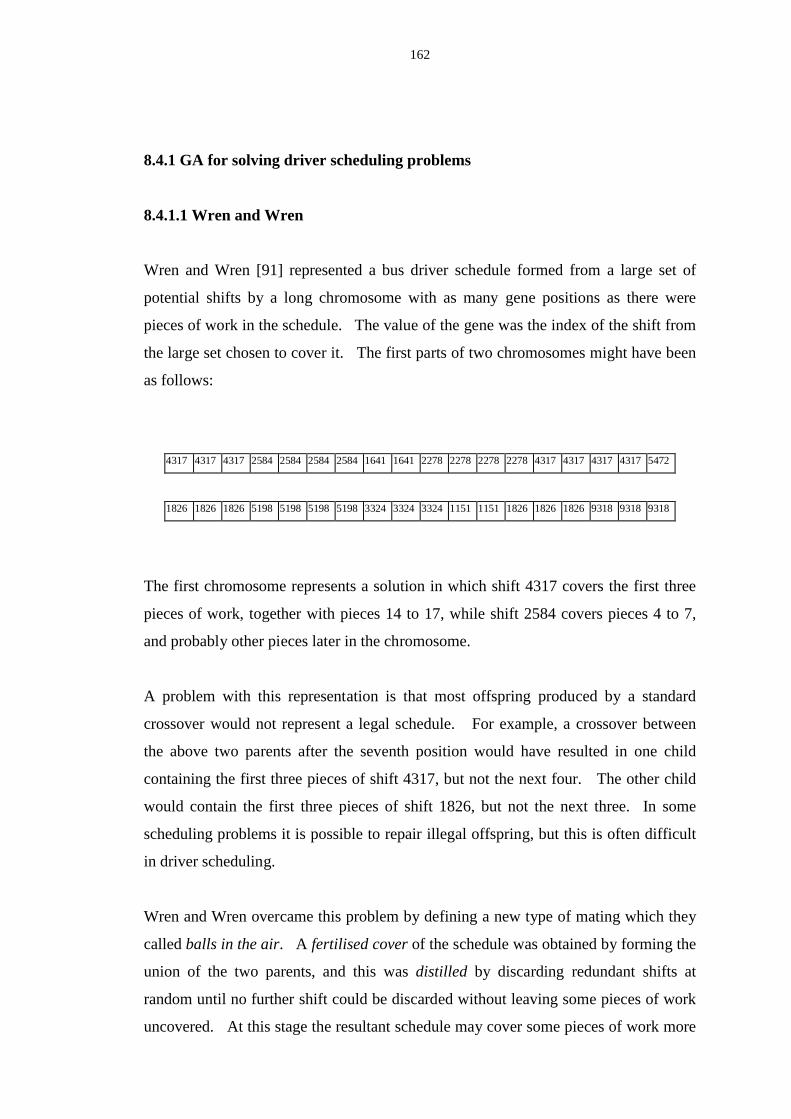
162
8.4.1 GA for solving driver scheduling problems
8.4.1.1Wren and Wren
Wren and Wren [91] represented a bus driver schedule formed from a large set of
potential shifts by a long chromosome with as many gene positions as there were
pieces of work in the schedule. The value of the gene was the index of the shift from
the large set chosen to cover it. The first parts of two chromosomes might have been
as follows:
4317 4317 4317 2584 2584 2584 2584 1641 1641 2278 2278 2278 2278 4317 4317 4317 4317 5472
1826 1826 1826 5198 5198 5198 5198 3324 3324 3324 1151 1151 1826 1826 1826 9318 9318 9318
The first chromosome represents a solution in which shift 4317 covers the first three
pieces of work, together with pieces 14 to 17, while shift 2584 covers pieces 4 to 7,
and probably other pieces later in the chromosome.
A problem with this representation is that most offspring produced by a standard
crossover would not represent a legal schedule. For example, a crossover between
the above two parents after the seventh position would have resulted in one child
containing the first three pieces of shift 4317, but not the next four. The other child
would contain the first three pieces of shift 1826, but not the next three. In some
scheduling problems it is possible to repair illegal offspring, but this is often difficult
in driver scheduling.
Wren and Wren overcame this problem by defining a new type of mating which they
called balls in the air. A fertilised cover of the schedule was obtained by forming the
union of the two parents, and this was distilled by discarding redundant shifts at
random until no further shift could be discarded without leaving some pieces of work
uncovered. At this stage the resultant schedule may cover some pieces of work more

163
than once (indeed this was allowed in the initial population members); however,
overlapping shifts can be cut back to provide a legal schedule.
Although this work started by considering chromosomes as defined above, in practice
the chromosome can be represented by a list of the shifts contained in it. This is more
concise and lends itself easily to forming the union of parents. The GA described by
Wren and Wren uses a ‘steady-state’ approach which is different from the traditional
‘generational replacement’ GA as defined by Holland [85]. A ‘steady-state’ GA
replaces only a few individuals at a time, rather than replacing the entire population at
each generation (‘generational replacement’). In a steady-state GA, both parents and
their offspring are allowed to coexist in the same population. Wren and Wren
discovered that on average the children were fitter than the parents, and they obtained
best results by mating three parents in this way, rather than two. Good schedules
were consistently obtained using randomly generated starting solutions for a small
problem requiring sixteen shifts. However, subsequent work on significantly larger
problems failed to find good solutions.
8.4.1.2 Clement and Wren
The chromosome structure of the GA described by Clement and Wren [86] is the
same as the one used in Wren and Wren. Clement and Wren describe using various
strategies on crossover and mutation in order to improve the quality of the GA
solutions. Each population member is a feasible driver schedule. Two parents are
chosen and their shifts are combined to form a ‘fertilised’ set. A new schedule will be
produced by covering pieces of work in turn by selecting shifts from this ‘fertilised’
set. They use various crossover algorithms and conclude that using a permutated
greedy crossover algorithm combined with an optimising mutation gives the best
results. In a permutated greedy crossover algorithm, pieces of uncovered work will
be chosen randomly and, using a greedy approach, the shift that covers most
uncovered work will be chosen from the ‘ fertilised’ set.
They found that classical mutation which occasionally changed the gene value in a
chromosome had a negative effective both on the performance and the quality of
solution. They argue that randomly changing the gene values very rarely produces a

164
better individual. Instead, they opt for an optimising mutation which is similar to a
local search. It inspects the input set of shifts and selects one or more shifts and
exchanges shifts in the individual with shifts from the input shift set making sure that
the changed solution is better than before. Clement et al present results from various
versions of GA using different crossover and mutation algorithms and the results are
reported to have a few shifts more than the known best solutions obtained from an
ILP process. The fact that there exists an enormous search space and there is no
means of directing the GA search to a more promising area results in the GA
converging to a sub-optimal solution very quickly.
8.4.1.3Hernandez and Corne
Hernandez and Corne [92] developed an algorithm using a divide and conquer
approach for the set covering problem and applied it to three general set covering
instances and a driver scheduling problem provided by the group at Leeds. They
divide the problems into several sub-problems by fragmenting a chromosome into
smaller contiguous segments. The new sub-problems are each allocated a sub-
population that will evolve independently. Individuals from each sub-populations are
chosen and combined to form an overall solution. They use a chromosome similar to
Wren and Wren above, with a gene position for each piece of work, but they use an
overcovered schedule in which it is not necessary for any shift to be indicated in all
the gene positions which it covers. Thus in the above example, shift 4317 might
appear in the first gene position, shift 1826 in the second, and either of these, or some
other shift in the third. This representation is similar in many ways to the fertilised
cover of Wren and Wren, and an actual schedule is extracted from the chromosome
by a distillation process like that of Wren and Wren, leading to a cover of the
schedule which contains no redundant shift, but may contain overcovered pieces of
work.
Offspring may be generated using Hernandez and Corne’s representation using a
simple crossover; the solution is always legal, and the corresponding schedule may be
obtained by distillation. There are of course generally many possible corresponding
schedules, depending on the random nature of the distillation process, and fitness was
defined as the mean of several distilled schedules. They presented results which show
165
the impact of using different number of pools used to break the problem down. There
is no direct comparison with the results obtained by other GA's or other methods.
8.4.1.4Beasley and Chu
Beasley and Chu [93] used a chromosome structure in which each gene position
represents one of the possible covering variables (driver shifts in our problem), and
has a value of 1 or 0 depending on whether the variable is or is not present in the
solution. Crossover operators lead to an infeasible solution which they then repair.
They use a ‘ fusion’ operator for crossover which is bias on the fitness of the
individual parents. A fusion operation is that when combining two parent strings, the
choice of whose gene values are passed to the child should be made based on the
relative fitness of the two parents.
Chu used a variable mutation rate which depends on the rate at which the GA
converges. At an initial stage of the GA, the mutation rate is set at a low value to
allow minimal disruption. As the GA progresses, the crossover operator becomes less
effective and so the mutation rate increases. When the GA finally converges, the
mutation rate will stay at some constant rate.
This process has been successfully applied to air crew scheduling problems among
others, but it is believed that these are easier to solve by this approach than train or
bus driver scheduling problems because the normal air crew duty has fewer separate
pieces than the average train or bus driver shift, and there are not as many possible
distinct shifts.
8.4.2 A parallel GA for the set partitioning problem
Levine [94] describes a parallel genetic algorithm and applied it to the set partitioning
problem. The chromosome representation used is the traditional one: a gene in a
chromosome is associated with each column j. The gene has value ‘1’ if column j is
included in the solution, and zero otherwise. The GA described by Levine also uses a
‘steady-state’ approach for population replacement. The GA is hybridised with a
166
local search heuristic which is row-oriented in order to improve the current solution
which might or might not be feasible. The heuristic described uses a first-improving
strategy in which randomness is introduced through the local search. The evaluation
function is based on the cost of the solution plus a penalty which depends on the
infeasibility of the solution. Selection is based on a binary tournament. Uniform
crossover is used for combining chromosomes to form offspring.
The above GA is then implemented as a parallel GA based on an ‘ Island Model’
where separate and isolated sub-populations evolve independently and in parallel.
Occasionally, fit population members migrate between sub-populations. This
migration between sub-populations allows the distribution and sharing of good
genetic material of fit members and helps to maintain genetic diversity.
For small problems with fewer than 100 rows and 7000 columns, the GA described
can find the best solutions for the problem instances. He concludes that the larger the
number of sub-problems, the higher the chance that an optimal solution can be found.
For larger problem instances (between 100 to 823 rows), the GA has diffi culty in
finding any feasible solution.
8.4.3 Using GA for relief opportunities selection
Kwan and Wren [95] explored an alternative use of a GA in bus driver scheduling.
Their GA process is to select relief opportunities from the full set which may be used
as the basis for TRACS II or for a GA as above. De-selecting some relief
opportunities of the problem will effectively decrease the number of rows in the ILP
model and hence decrease the problem size. A binary chromosome represents the
entire set of potential relief opportunities. A ‘1’ in any gene position indicates that the
associated relief opportunity is selected and a ‘0’ indicates otherwise.
A relatively accurate process for estimating the number of shifts required for any bus
schedule was developed by Zhao, Wren and Kwan [96, 97]. This estimator is used to
assess the likely number of shifts which will be required to form a schedule based on
the relief opportunities retained in the chromosome, and is thus a measure of the
fitness of the chromosome.
167
The population is allowed to evolve using single crossovers, and offspring are
evaluated by the estimator. The GA will terminate when most members of the
population have a fitness equal to that of the full set of relief opportunities. A union
of the opportunities present in a selection of population members is presented to the
IMPACS driver scheduling system.
In this approach, a GA is used as a pre-processor to reduce the problem size. It does
not solve the driver scheduling problem on its own. Its success depends on the
accuracy of the estimator, which analyses mealbreak chains quite extensively.
8.4.4 A new approach relating to GA
A new concept derived from GA has evolved in the past few years and is known as a
memetic algorithm. This approach was presented by Moscato and Norman [98] and
later by Radcliffe and Surrey [99]. A meme is a unit of information that reproduces
itself as people exchange ideas. Basically, a memetic algorithm is an evolutionary
algorithm combined with local search. A meme differs from a gene in that the meme
is passed between population members and each member adapts the meme as it sees
best whereas genes are passed unaltered. Compared with a GA which mimics a
biological evolution, a memetic algorithm models a cultural evolution, i.e. an
evolution of ideas. The main advantage of using memetic algorithms is that the search
space is reduced to the subspace of local optima. Burke et al [100] describe a
multistage memetic algorithm for solving university examination timetabling
problems.
The use of local search in the GA process will increase the computational cost and the
complexity of the GA for driver scheduling problems. Given the complexity of the
GA which will be described in the next chapter, this approach has not been pursued in
this research.
8.5 Identifyi ng important combinatorial traits
As a standard GA progresses, some fitter members are becoming dominant over the
others. These fitter members are those whose solutions are better than the others in
168
terms of number of shifts and total cost. This research aims at identifying within
these elite members key patterns of work piece combinations that have enabled the
schedules to become superior to the others. We call such patterns and characteristics
combinatorial traits. Various bus driver scheduling systems described in Chapter
Two (e.g. HOT and TRACS) use heuristic rules concerning combinatorial traits, but
they are typically engaged in sequential searches involving only one schedule, or
partial schedule, at a time. In a GA, combinatorial traits can be propagated as genetic
materials and have effects on a population of schedules.
In previous research [86, 87, 91] using GA for driver scheduling problems, there has
been no attempt to manipulate combinatorial traits explicitly, which are left to chance
emergence within population members. Since combinatorial traits are undetected,
they cannot be used to influence the evolutionary process. This research seeks
dynamically to revise the chromosome structure to incorporate some combinatorial
traits as genetic materials so that they will also be subject to the survival-of-the-fittest
principle. Inherited traits will directly affect the way a solution schedule is
constructed. The evolutionary approach has the advantage that weak combinatorial
traits arising from poor members will not be able to survive the evolution. However,
incorporating combinatorial traits into the GA process will no doubt increase the
GA’s complexity and may cause the GA to lose its ability to search a large area
effectively. Hence only combinatorial traits that have a positive effect on the GA
should be implemented. The two combinatorial traits, preferred shifts of the relaxed
LP; relief chain are identified and have been implemented into our GA. These traits
are found to be effective means of helping the GA to converge to good solutions.
Other combinatorial traits identified will be discussed in the Section 9.6.2 as possible
future work.
8.5.1 Preferred shifts
8.5.1.1 The relaxed LP solution
Provided that the input to the LP process is within the limits of our LP solver and
there is no presence of any user-specified side constraints, it is always able to obtain a
relaxed solution after the re-optimised stage of the primal phase (Step 5 of Section

169
7.2.1.1). It is often the branch and bound stage that gives rise to the problem of not
being able to find an integer solution. After the integer relaxation phase, the relaxed
solution found can provide us with some useful information about the significance of
some of the shifts identified in the relaxed solution. Research into the properties of
the relaxed solution (see below) confirms that the relaxed solution on average
contains about three quarters of the shifts found in the integer solution. Some of the
shifts involved in the non-integer solution, which is a relatively small set compared to
the initial input set, therefore fit well together.
8.5.1.2 Preferred shifts identified in the relaxed solution
The relaxed solution provides two pieces of useful information. First, the sum of all
the shift variables, xj (rounded up if the fractional part is non-zero) is a very accurate
estimation of the lower bound of the number of shifts required in the integer solution.
More importantly, it is a general property of LP's that the relaxed solution will involve
a (relatively small) number of shifts that is no more than the total number of work
piece constraints plus any side constraints. The corresponding variables for some of
these shifts may have values of one or zero, but most of them will have fractional
values. It is observed that often some of these shifts are used in the final integer
solution, and hence they should be crucial to the formation of a good integer solution.
Twenty-three sets data have been used to find the proportion of the shifts present in
the relaxed solution that are also present in the integer solution obtained by the branch
and bound. The results are shown in Table 8.1.
Column (a) of Table 8.1 shows the number of shifts involved as basic variables in the
relaxed solution. Basic variables consist of shift variables and surplus variable and
here we are only interested in the shift variables. These shifts all have fractional
values and some of their fractional values are zeroes. Column (b) shows the number
of shifts in the integer solution found in the subsequent branch and bound phase.
Column (c) shows the number of shifts that are present both in the integer solution
and in the relaxed solution shift set. The next column shows the percentage of (c) that
are in (b) and the average percentage is as high as 79%. In some cases, almost all the
shifts used in the integer solution are already present in the relaxed solution (G5X,

170
EXNR, WKH). Since there may be many different integer solutions using the
minimum number of shifts, those shifts in the relaxed solution but not in the integer
solution returned by the ILP may still be used in a different integer solution with a
minimum shifts schedule.
Data set No. of shifts (c) / (b) ××100 % Total no. of No. of
(a) Relaxed (b) Integer (c) Common shift work
soluti on* solution In (a) and (b) variables pieces
G34A 476 106 70 66 30701 502
G14A 268 61 41 67 31913 372
G149 307 65 43 66 30510 372
EXNR 216 74 71 96 11950 236
ALL 358 87 51 59 29743 454
G309 425 113 76 67 27973 502
W7 281 61 52 85 29995 297
W3 237 52 41 79 29913 256
WAKH 428 106 88 83 30000 446
SWAX 321 48 32 67 30574 339
SWBX 474 132 104 79 30423 632
WKH 420 109 98 90 30000 468
MON 220 49 33 67 20761 222
TLXX 392 112 100 89 14818 537
TLYY 377 112 99 88 22917 538
G209 361 95 69 73 22000 454
GMB 135 34 23 68 11817 154
G5X 189 42 40 95 12343 196
R207 225 40 31 78 11451 244
GW01 354 89 69 78 29380 359
HE01 159+ 14 8 57 27542 158
G32X 902 214 160 75 29052 926
WAG3 360 50 42 84 16636 400
Average = 78.8
Table 8.1: Relationship of shifts in an integer solution and those in the relaxed solution
* The shifts here include shifts with ‘zero’ fractional values.+ The LP problem contains more than one side constraints.
The results in Table 8.1 indicate that a subset of the shifts identified in the relaxed
solution could be crucial in forming the subsequent integer solution because they tend
to fit well. Each such subset could constitute a ‘combinatorial trait’. We therefore
171
proceeded to develop a GA to derive such subsets. Each subset will be supplemented
with shifts selected from the original large pool of potential shifts to form a schedule.
Thus the GA will also be yielding indirectly a population of complete schedules. It is
expected that each schedule will pass on its own traits to the next generation. Those
surviving the evolution process will possess characteristics that enable them to
survive.
The shifts in the relaxed solution are referred to as the preferred shifts, which is a
much smaller set than the full set of shifts at the start of the mathematical process.
The full set of shifts are referred to as potential shifts. Roughly, there are three
classes of preferred shifts: (i) those with zero value; (ii) those with fractional value;
(iii) those with value '1'. Further investigation revealed that the fractional values of
the preferred shifts may give an indication as to how likely the preferred shift is to be
present in an integer solution. It is found that the higher the fractional value of the
preferred shifts, the higher the chance that they are present in the integer solution.
The results of such an investigation are found in Tables 9.1 and 9.2 in the next
chapter.
In summary, the relaxed solution can provide the following information which can
help to initiate the GA process and limit the search space:
1. A list of preferred shifts, which have high chances of being used in the best
integer solution.
2. A lower bound on the minimum number of shifts, which can be one of the
termination criteria for a GA.
8.5.2 Relief chain
An important feature in driver scheduling is that driver shifts have one or more
breaks, e.g. for having a meal, in them. After a break, the driver is usually assigned to
work on another vehicle, often taking over from another driver who is due for a break.
Thus a chain of events of drivers relieving each other is formed, and we call the relief

172
opportunities involved a “relief chain”. For example, Figure 8.2 shows a relief chain
(R1 - R2 - R3). Shift 1 starts its break at R1, relieves shift 2 when it resumes work at
R2. Shift 2 relieves shift 3 when it resumes work at R3.
R1
R2
R3
Shift 2
Shift 1
Shift 1
Shift 3
Shift 3
Shift 2
Figure 8.2: A relief chain R1 - R2 - R3
Relief chains have been the subject of much investigation in previous research into
driver scheduling heuristics. Fores [9] explored the possibility of using mathematical
programming methods to create a schedule based solely on systematically forming
mealbreak chains. Experience suggests that well formed relief chains, especially
critical during peak periods, can avoid using extra drivers unnecessarily. In Figure
8.3, the two relief chains, T and S, both represent efficient ways to relieve drivers who
are due for their meal relief to be relieved by drivers who have finished mealbreaks as
opposed to new drivers. In each case, five shifts start at the beginning of the vehicles;
a sixth shift T6 starts on vehicle 303 if chain T is used, while a sixth shift S6 starts on
vehicle 301 if chain S is used.
It should be noted that in some cases although two relief chains may be different, one
of the chains may be shifted from the other by roughly the same amount of time along
the chain as shown in Figure 8.3. Here, the horizontal lines represent the work of
vehicles 301 to 305 drawn to timescale and are truncated at the right hand side. The
relief opportunities are marked with the letter "o". Parts of two schedules, whose
shifts are labelled by numbers with prefixes S and T respectively, are shown, one
above and the other below the horizontal line. The "+" signs delimit the work covered
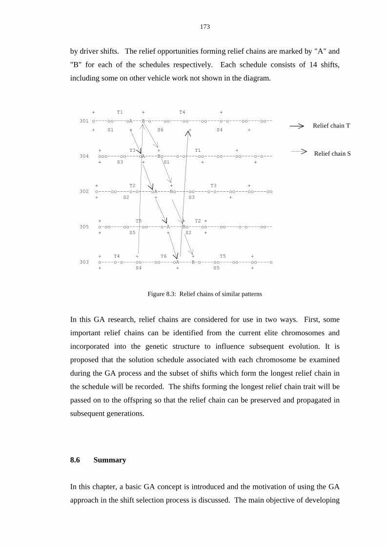
173
by driver shifts. The relief opportunities forming relief chains are marked by "A" and
"B" for each of the schedules respectively. Each schedule consists of 14 shifts,
including some on other vehicle work not shown in the diagram.
+ T1 + T4 +
301 o---- oo---- oA---B-o---- oo----oo---- oo----o-o---- oo---- oo--
+ S1 + S6 + S4 +
+ T3 + T1 + 304 ooo---- oo---- oA----Bo----o-o---- oo----oo---- oo----o-o--- + S3 + S1 + +
+ T2 + T3 + 302 o---- oo----o-o---- oA----Bo---- oo----o-o---- oo----oo---- oo + S2 + S3 +
+ T5 + T2 + 305 o- oo----oo---- oo----o-A----Bo---- oo---- oo----o-o---- oo-- + S5 + S2 +
+ T4 + T6 + T5 + 303 o----o-o---- oo----oo---- oA----B-o---- oo----oo---- oo----o + S4 + S5 +
Figure 8.3: Relief chains of similar patterns
In this GA research, relief chains are considered for use in two ways. First, some
important relief chains can be identified from the current elite chromosomes and
incorporated into the genetic structure to influence subsequent evolution. It is
proposed that the solution schedule associated with each chromosome be examined
during the GA process and the subset of shifts which form the longest relief chain in
the schedule will be recorded. The shifts forming the longest relief chain trait will be
passed on to the offspring so that the relief chain can be preserved and propagated in
subsequent generations.
8.6 Summary
In this chapter, a basic GA concept is introduced and the motivation of using the GA
approach in the shift selection process is discussed. The main objective of developing
Relief chain T
Relief chain S

174
a GA is to replace the branch and bound of the ILP process so that a solution can
always be guaranteed. Various works relating to using GA for driver scheduling
problems are reviewed. In order to devise a GA that can search for a good solution
effectively, the concept of identifying and implementing combinatorial traits into the
GA is explained. Two combinatorial traits are identified and described in detail. The
next chapter will discuss the GA implementation with embedded combinatorial traits
and the test results.
175
Chapter Nine
A GA with embedded combinatorial traits
9.1 Introduction
This chapter describes a GA developed by the author which features genetic
propagation of the combinatorial traits identified in Chapter Eight. The GA has been
used on a number of real life train and bus driver scheduling problems and the results
will be presented here. The chapter will present a conclusion of using the GA
developed in this research for shift selection followed by some suggestions on areas
of future work which may improve the present GA.
Throughout this GA research, user-specified side constraints (except the ones
imposed on the ILP solver to increase the target number of shifts when a previous ILP
run fails to find a solution) are not used for both the GA and the ILP solver.
9.2 GA with embedded combinatorial traits
9.2.1 Using an LP solver for identifying the preferred shifts
In order to identify the preferred shifts from the relaxed solution, slight program
modification to the LP solver has to be made so that all preferred shifts and their

176
corresponding fractional values are output on a file. This GA research has used the
same version of the LP solver throughout. This LP solver is called PENZIP which is
a version derived from the original ZIP package [73] used in IMPACS and it is
without Wil lers’ [8] and Fores’ [9] enhancements of the latest LP solver used in
TRACS II . The maximum number of potential shifts (columns) input to PENZIP is
30,000. All the relaxed solutions available for the GA research are based on the
results from PENZIP. The BUILD process of TRACS II creates the potential shifts.
If there are more than 30,000 shifts created by BUILD (see Chapter Five), the shift set
is reduced by using the process SIEVE. Figure 9.1 shows how the GA model
interfaces with PENZIP and TRACS II .
TRACS II
Figure 9.1: Interface between TRACS II and GA
The GA model proposed here requires the input potential shift set produced by
BUILD and a subset of shifts identified as the preferred shifts in the relaxed solution
of the LP process. After solving the problem as a set covering problem, the GA
outputs the best ten schedules found in the population.
9.2.2 Chromosome representation using the preferred shifts
The first step in designing a GA is to devise a suitable representation scheme for the
problem. There are several representation schemes which have been explored by other
GAprocess
ShiftGeneration
Preferred shiftsand target
Potential shifts
RelaxedPhase
Branch andBound Phase
Shift SelectionPENZIP
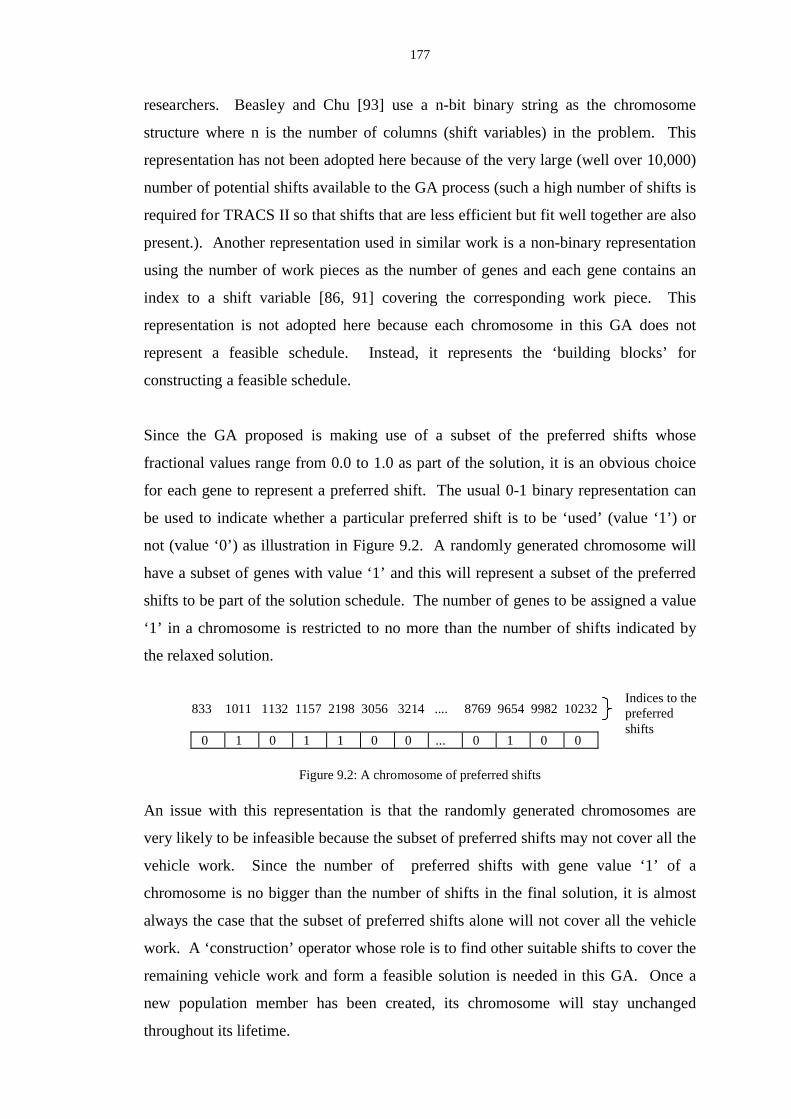
177
researchers. Beasley and Chu [93] use a n-bit binary string as the chromosome
structure where n is the number of columns (shift variables) in the problem. This
representation has not been adopted here because of the very large (well over 10,000)
number of potential shifts available to the GA process (such a high number of shifts is
required for TRACS II so that shifts that are less efficient but fit well together are also
present.). Another representation used in similar work is a non-binary representation
using the number of work pieces as the number of genes and each gene contains an
index to a shift variable [86, 91] covering the corresponding work piece. This
representation is not adopted here because each chromosome in this GA does not
represent a feasible schedule. Instead, it represents the ‘building blocks’ for
constructing a feasible schedule.
Since the GA proposed is making use of a subset of the preferred shifts whose
fractional values range from 0.0 to 1.0 as part of the solution, it is an obvious choice
for each gene to represent a preferred shift. The usual 0-1 binary representation can
be used to indicate whether a particular preferred shift is to be ‘used’ (value ‘1’) or
not (value ‘0’) as illustration in Figure 9.2. A randomly generated chromosome will
have a subset of genes with value ‘1’ and this will represent a subset of the preferred
shifts to be part of the solution schedule. The number of genes to be assigned a value
‘1’ in a chromosome is restricted to no more than the number of shifts indicated by
the relaxed solution.
833 1011 1132 1157 2198 3056 3214 .... 8769 9654 9982 10232
0 1 0 1 1 0 0 ... 0 1 0 0
Figure 9.2: A chromosome of preferred shif ts
An issue with this representation is that the randomly generated chromosomes are
very likely to be infeasible because the subset of preferred shifts may not cover all the
vehicle work. Since the number of preferred shifts with gene value ‘1’ of a
chromosome is no bigger than the number of shifts in the final solution, it is almost
always the case that the subset of preferred shifts alone will not cover all the vehicle
work. A ‘construction’ operator whose role is to find other suitable shifts to cover the
remaining vehicle work and form a feasible solution is needed in this GA. Once a
new population member has been created, its chromosome will stay unchanged
throughout its lifetime.
Indices to thepreferredshifts
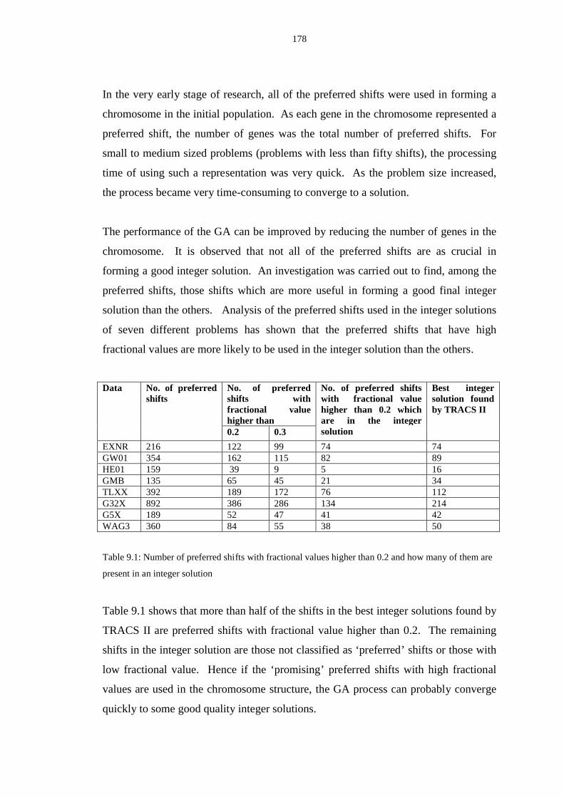
178
In the very early stage of research, all of the preferred shifts were used in forming a
chromosome in the initial population. As each gene in the chromosome represented a
preferred shift, the number of genes was the total number of preferred shifts. For
small to medium sized problems (problems with less than fift y shifts), the processing
time of using such a representation was very quick. As the problem size increased,
the process became very time-consuming to converge to a solution.
The performance of the GA can be improved by reducing the number of genes in the
chromosome. It is observed that not all of the preferred shifts are as crucial in
forming a good integer solution. An investigation was carried out to find, among the
preferred shifts, those shifts which are more useful in forming a good final integer
solution than the others. Analysis of the preferred shifts used in the integer solutions
of seven different problems has shown that the preferred shifts that have high
fractional values are more likely to be used in the integer solution than the others.
No. of preferredshifts withfractional valuehigher than
Data No. of preferredshifts
0.2 0.3
No. of preferred shiftswith fractional valuehigher than 0.2 whichare in the integersolution
Best integersolution foundby TRACS II
EXNR 216 122 99 74 74GW01 354 162 115 82 89HE01 159 39 9 5 16GMB 135 65 45 21 34TLXX 392 189 172 76 112G32X 892 386 286 134 214G5X 189 52 47 41 42WAG3 360 84 55 38 50
Table 9.1: Number of preferred shifts with fractional values higher than 0.2 and how many of them are
present in an integer solution
Table 9.1 shows that more than half of the shifts in the best integer solutions found by
TRACS II are preferred shifts with fractional value higher than 0.2. The remaining
shifts in the integer solution are those not classified as ‘preferred’ shifts or those with
low fractional value. Hence if the ‘promising’ preferred shifts with high fractional
values are used in the chromosome structure, the GA process can probably converge
quickly to some good quality integer solutions.

179
Table 9.2 shows an extract of a problem solved by PENZIP with an integer solution of
116 shifts in which 89 shifts are from the preferred shift set together with their
corresponding fractional value in the continuous solution.
Fractional values inrelaxed solution
No. of preferred shifts No. of preferred shifts inthe integer solution
0.00 - 0.09 204 50.10 – 0.24 11 30.25 – 0.49 44 50.50 – 0.74 64 160.75 – 0.99 13 61.00 61 54Total 407 89
Table 9.2: Distribution of preferred shifts with respect to their fractional values
Table 9.2 shows that 5 out of the 204 preferred shifts whose fractional values are 0.00
– 0.09 are used in the integer solution; and 54 out of the 61 preferred shifts whose
fractional values are 1.00 are used in the integer solution. Hence the number of genes
can be reduced by choosing only a portion of the preferred shifts which are likely to
be used in the integer solution. A selection criterion is therefore implemented in the
GA in which a parameter can be used as the desired fractional values so that only
those preferred shifts with fractional values higher than the parameter are to be chosen
as genes. This parameter is one of the system parameters to be supplied externally.
There is obviously a risk that if the preferred shifts with low fractional values are not
part of the gene structure, the quality of solution of the GA may be affected. While
such a risk is possible, the genes in the chromosome only form part of the solution
and the remaining shifts of the solution are to be found by the ‘construction’ operator
which will select shifts from a much larger pool of potential shifts than from the
preferred shifts. Various experiments using this selection criterion showed that by
selecting preferred shifts with fractional values above the range of between 0.2 to 0.3
does improve both the running time and the quality of the solutions.
9.2.3 Random creation of a chromosome
Chromosomes are created randomly for the initial population and for replacing a
certain proportion of the population at the end of each generation. If g is the number
of preferred shifts whose fractional values are higher than a minimum parameter, each

180
chromosome will have g genes. The process selects a certain number, r, of these g
genes to have value ‘1’ and sets the rest to ‘0’. A ‘1’ indicates that the corresponding
preferred shift is to be included in the solution set represented by the chromosome.
This number, r, is set randomly to be between 0.0 to 25% of the target. Other ranges
(0.0 – 50%, 0.0 – 75%) have been tried and 0.0 to 25% seems to produce the best
results and hence is adopted. The process will randomly select r genes of this
chromosome to have value ‘1’. As the evolution progresses, the number of genes
with value ‘1’ in the chromosomes should increase because the children will inherit
genes from the parents.
9.2.4 Reducing the number of potential shifts to reduce problem size
A proven shift reduction heuristic used in TRACS II which has been described in
Section 7.2.1.3 is adopted here in order to reduce the GA search space. The reduction
technique assumes that an acceptable integer solution can be found by restricting the
choice of relief times to only those used by the set of preferred shifts. Any shift
which uses a relief time not being used by any of the preferred shifts is banned. The
reduction technique is a standard feature of TRACS II which has been successful in
reducing the problem size and producing good integer solutions.
This reduction technique helps to cut down the number of potential shifts and reduce
the search space enormously. Table 9.3 shows the large number of shifts banned by
the reduction heuristic. This technique is incorporated into our GA process. For
smaller problems, this technique is less useful as the amount of time saved in solving
the problem is insignificant. Hence the technique is implemented as an optional
feature.
Data Number ofpotentialshifts input
No. of shifts with inthe relaxedsolution (preferredshifts)
Number ofpotentialshiftsbanned
Best integersolution foundby TRACS
EXNR 11950 216 6355 74GW01 29380 354 14930 89HE01 27542 159 25336 16GMB 11817 135 5955 34TLXX 14818 392 11205 112G32X 29052 892 11810 214G5X 12343 189 11318 42WAG3 16636 360 13923 50
Table 9.3: Use of shift reduction heuristic to reduce the search space
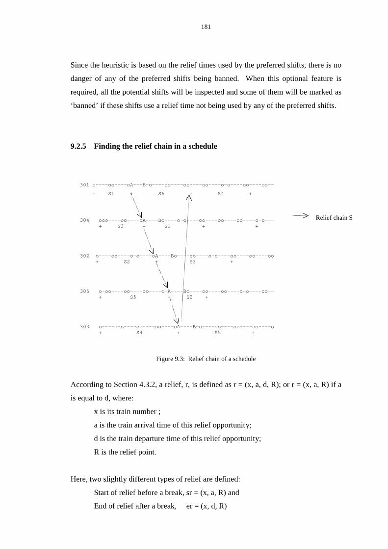
181
Since the heuristic is based on the relief times used by the preferred shifts, there is no
danger of any of the preferred shifts being banned. When this optional feature is
required, all the potential shifts will be inspected and some of them will be marked as
‘banned’ if these shifts use a relief time not being used by any of the preferred shifts.
9.2.5 Finding the relief chain in a schedule
301 o---- oo---- oA---B-o---- oo----oo---- oo----o-o---- oo---- oo--
+ S1 + S6 + S4 +
304 ooo---- oo---- oA----Bo----o-o---- oo----oo---- oo----o-o--- + S3 + S1 + +
302 o---- oo----o-o---- oA----Bo---- oo----o-o---- oo----oo---- oo + S2 + S3 +
305 o- oo----oo---- oo----o-A----Bo---- oo---- oo----o-o---- oo-- + S5 + S2 +
303 o----o-o---- oo----oo---- oA----B-o---- oo----oo---- oo----o + S4 + S5 +
Figure 9.3: Relief chain of a schedule
According to Section 4.3.2, a relief, r, is defined as r = (x, a, d, R); or r = (x, a, R) if a
is equal to d, where:
x is its train number ;
a is the train arrival time of this relief opportunity;
d is the train departure time of this relief opportunity;
R is the relief point.
Here, two slightly different types of relief are defined:
Start of relief before a break, sr = (x, a, R) and
End of relief after a break, er = (x, d, R)
Relief chain S

182
In a solution schedule, a break, ß, is made up by two relief opportunities, sr, er and a
shift number, y which contains the break, i.e. ß = (sr, er, y). A set of breaks, B,
contains all the breaks identified in a schedule. A relief chain shifts set is the set, c
which contains a list of shifts forming a relief chain. There are usually a number of
chains identified in a schedule. In order to form all the possible relief chains in a
schedule like the one shown in Figure 9.3, the following algorithm is used:
1. Sort the breaks in B in ascending order of their start times, a;
2. i = 1; // index to ß in B
3. k = 0 ; //index to the relief chains formed
4. If ßi has not been included in any chain formed
k = k + 1;
ck ← yi;
Repeat
j = i+1; //next available ß in B
if (eri = srj )
ck ← yj; // a chain is formed
remove ßi if it has not been removed ;
remove ßj from B;
else
j = j + 1;
end-if
Until j = last ß in B
5. if B is empty, stop
6. i = next available break in B and goto 3;
After all the chains have been formed, the relief chain shifts set with the largest
number of shifts, i.e. the longest chain, will be stored with the shifts that made up this
longest chain. After a crossover, each child will receive a set of relief chain shifts
from each parent and these shifts are then put into the solution set associated with the
child's chromosome. These shifts together with the preferred shifts indicated by the
child's chromosome will form the initial shift set of a feasible schedule.
183
9.2.6 The GA
A population member has the following attributes:
1. a chromosome
2. a solution schedule whose constitution is based on the genes of the chromosome
and/or the shifts present in the relief chain inherited
3. a list of shifts which forms the longest relief chain in the solution (the list is empty
if the chromosome is created randomly for the initial population or population
replacement)
4. ‘unfitness’ value derived from the solution
Step 1:
Run PENZIP up to the revised relaxed phase but before branch-and-bound phase to
create a list of preferred shifts with their fractional values and the number of preferred
shift is p. PENZIP will also provide a target total, T, for the final solution.
Step 2:
If requested, use the ‘shifts reduction technique’ (Section 8.6.2) to ban some potentialshifts
Step 3:
Select from the preferred shifts a subset of shifts whose fractional values are above a
parameter, c. This creates a set of selected preferred shifts, the total number is s.
The number of genes in each chromosome is therefore s.
Step 4 (Steps 4 to 6 are for the creation of a new population member):
Randomly generate a number, q, between 0 and T/4, q genes of the chromosome will
have a gene value ‘1’. This means the corresponding selected shifts are to be used to
build a solution.
Step 5:
Complete the solution set by using a construction operator. (See Section 9.2.7)
Compute the ‘unfitness’ of the population member from the solution set.

184
Find the longest relief chain present in the solution set and store the relevant shifts
which are called ‘relief chain shifts’
Step 6
If the required population size is not reached, go to step 4, otherwise, perform Step 7
to 10 (the evolution process).
Step 7 (Step 7 to Step 10 are the evolution process):
If the required number of generations has not been reached and the solution has not
converged, continue with the following steps; otherwise stop the process.
Step 8 (crossover):
Randomly, but biased on fitter members, choose two members for single point
crossover. This will create two new children with different chromosomes, and each
inherits one of their parents’ relief chain shifts (Section 9.2.9) by including all the
shifts present in the parent’s chain into the child’s solution set.
If mutation is required, mutate both the children, otherwise continue (Section 9.2.10).
Similar to step 5 and for each child, construct a solution set, find the unfitness and
then find the relief chain shifts.
Step 9:
Newly created children are kept separate from the parents’ population.
If the required number of crossovers has been performed, one generation of evolution
is complete, goto Step 10; otherwise repeat Step 8.
Step 10:
Select a proportion of the fittest members from the combined parents and children
population and carry them forward to a new population.
New population members will be created at random (repeat steps 4 to 6) to replenish
the population to full size.
Goto Step 7.

185
9.2.7 The construction operator
The solution shifts set of any chromosomes created randomly will contain a list of
preferred shifts indicated by a ‘1’ in the genes. These chromosomes do not have any
ancestors and therefore do not have additional inherited relief chain shifts. The
solution shifts set of the children chromosomes always contains the list of inherited
relief chain shifts in addition to the list of preferred shifts. In almost all cases, the
preferred shifts from the chromosome together with the possible relief chain shifts are
unlikely to be able to cover all the work pieces. A construction operator is therefore
used to derive a valid solution schedule for these chromosomes.
The operator is called ‘construction’ rather than ‘repair’ because it only constructs a
valid schedule without changing the composition of the genes and hence there is no
repair work done to the chromosome. A ‘valid schedule’ is a schedule in which every
piece of work is covered by at least one shift and overcover (i.e. pieces of work being
covered by more than one shift) is allowed. The derived schedule is evaluated to
determine the fitness of its associated chromosome.
The construction operator contains two processes called FILL and DISCARD which
are executed once (FILL followed by DISCARD) for each chromosome. These
processes use heuristics which are adaptive in nature because the heuristic updates
information about the coverage of each work piece as shifts are inserted or deleted
from the schedule being formed. The information includes which shifts, if any, are
currently assigned to cover a particular piece of work. For each of the work pieces,
there is a list (called the coverage list) of all the unbanned potential shifts that can
cover it. A master coverage list is created at the beginning of the GA process and a
working copy of which is made for each chromosome.
FILL – a greedy, deterministic approach to adding shifts
For each piece of uncovered work, there will be at least one potential shift covering it.
All potential shifts are treated equally even if some of them are preferred shifts. The
heuristic used here will identify the piece of uncovered work which is covered by the
smallest number of potential shifts since it is the most critical piece of work to be

186
covered. Among these potential shifts, the one which covers most uncovered work
will be chosen. If V is the total amount of uncovered work covered by a shift variable
xj, the selection criterion is to maximise :
×= ∑=
m
1iijaV βi (9.1)
where aij = 1 if workpiece, currently uncovered, is covered by duty j, 0 otherwise;
βi = amount of work of workpiece i
In case of a tie, the one with a lower shift cost will be used. This potential shift will
be added to the solution shifts set of the chromosomes and the coverage statistics will
be updated. The process is repeated again on the next uncovered piece until all the
work is covered. When all the work pieces are covered, the solution shifts set will
have a feasible schedule which has a certain amount of work overcovered. The
additional shifts added by this process will not affect the gene structure of the
chromosome. It has been suggested that preferred shifts should be given preference
over the other shifts in the FILL process. However, the preferred shifts have already
played an important role in the genetic operations, such as crossover and mutation. It
is decided that it is better not to give preference to the preferred shifts so that the
construction operator will not interfere with the genetic structure of the chromosome.
DISCARD – removing redundant shifts
Before the construction operator is applied, many work pieces may already be
covered more than once by the selected preferred shifts and the relief chain shifts.
While the new shifts introduced by the FILL process will not be redundant
themselves, because each shift is chosen to cover an uncovered work piece, they may
increase the amount of overcover and cause some of the preferred shifts or the relief
chain shifts to become redundant. The DISCARD process aims to remove shifts that
are redundant.
The solution set will be scrutinised twice in order to remove unnecessary shifts. First,
the process will remove any redundant shifts which are not preferred shifts and make
sure that all the work is still covered. Second, the process will go through the solution
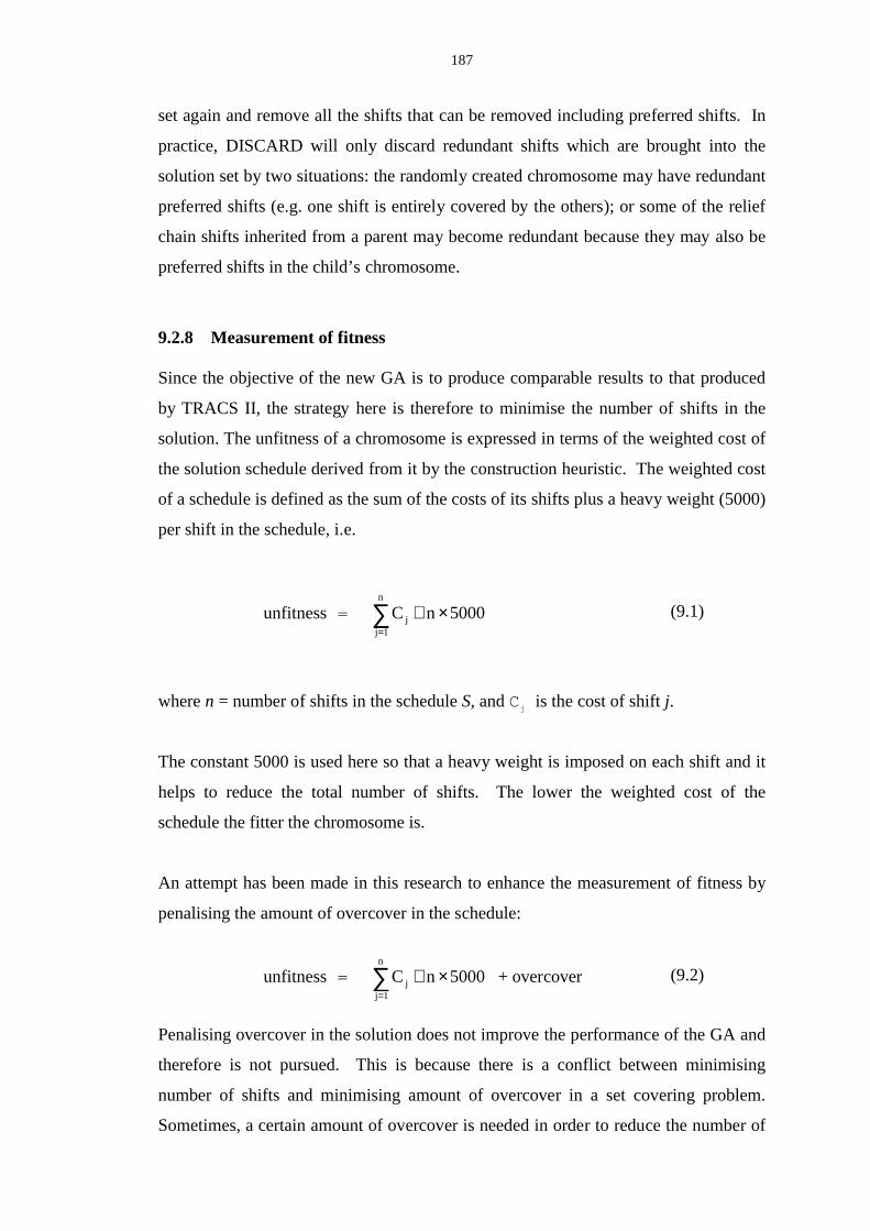
187
set again and remove all the shifts that can be removed including preferred shifts. In
practice, DISCARD will only discard redundant shifts which are brought into the
solution set by two situations: the randomly created chromosome may have redundant
preferred shifts (e.g. one shift is entirely covered by the others); or some of the relief
chain shifts inherited from a parent may become redundant because they may also be
preferred shifts in the child’s chromosome.
9.2.8 Measurement of fitness
Since the objective of the new GA is to produce comparable results to that produced
by TRACS II , the strategy here is therefore to minimise the number of shifts in the
solution. The unfitness of a chromosome is expressed in terms of the weighted cost of
the solution schedule derived from it by the construction heuristic. The weighted cost
of a schedule is defined as the sum of the costs of its shifts plus a heavy weight (5000)
per shift in the schedule, i.e.
unfitness = 5000nCn
1jj ×+∑
=
where n = number of shifts in the schedule S, and Cj is the cost of shift j.
The constant 5000 is used here so that a heavy weight is imposed on each shift and it
helps to reduce the total number of shifts. The lower the weighted cost of the
schedule the fitter the chromosome is.
An attempt has been made in this research to enhance the measurement of fitness by
penalising the amount of overcover in the schedule:
unfitness = 5000nCn
1jj ×+∑
=
+ overcover
Penalising overcover in the solution does not improve the performance of the GA and
therefore is not pursued. This is because there is a conflict between minimising
number of shifts and minimising amount of overcover in a set covering problem.
Sometimes, a certain amount of overcover is needed in order to reduce the number of
(9.1)
(9.2)
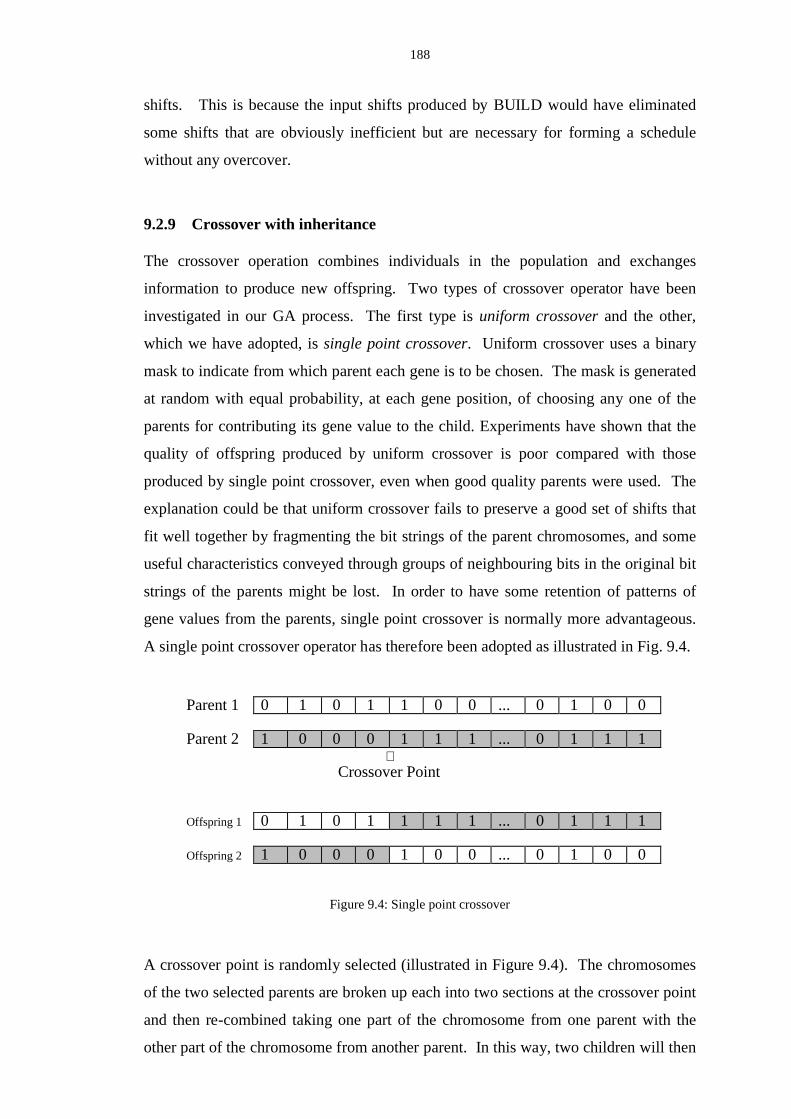
188
shifts. This is because the input shifts produced by BUILD would have eliminated
some shifts that are obviously inefficient but are necessary for forming a schedule
without any overcover.
9.2.9 Crossover with inheritance
The crossover operation combines individuals in the population and exchanges
information to produce new offspring. Two types of crossover operator have been
investigated in our GA process. The first type is uniform crossover and the other,
which we have adopted, is single point crossover. Uniform crossover uses a binary
mask to indicate from which parent each gene is to be chosen. The mask is generated
at random with equal probability, at each gene position, of choosing any one of the
parents for contributing its gene value to the child. Experiments have shown that the
quality of offspring produced by uniform crossover is poor compared with those
produced by single point crossover, even when good quality parents were used. The
explanation could be that uniform crossover fails to preserve a good set of shifts that
fit well together by fragmenting the bit strings of the parent chromosomes, and some
useful characteristics conveyed through groups of neighbouring bits in the original bit
strings of the parents might be lost. In order to have some retention of patterns of
gene values from the parents, single point crossover is normally more advantageous.
A single point crossover operator has therefore been adopted as illustrated in Fig. 9.4.
Parent 1 0 1 0 1 1 0 0 ... 0 1 0 0
Parent 2 1 0 0 0 1 1 1 ... 0 1 1 1⇑
Crossover Point
Offspring 1 0 1 0 1 1 1 1 ... 0 1 1 1
Offspring 2 1 0 0 0 1 0 0 ... 0 1 0 0
Figure 9.4: Single point crossover
A crossover point is randomly selected (illustrated in Figure 9.4). The chromosomes
of the two selected parents are broken up each into two sections at the crossover point
and then re-combined taking one part of the chromosome from one parent with the
other part of the chromosome from another parent. In this way, two children will then

189
be created. Apart from having two new chromosomes derived from both parents, the
newly created chromosomes also copy all the relief chain shifts from each parent into
their solution sets. One child inherits the relief chain set from one parent and the
other child from the other parent. Hence, all the population members created by
means of mating will always have such a trait inherited. The decision of which child
is to inherit from which parents is entirely random.
The construction operator constructs a solution set for each of the children. The effect
of imposing a relief chain on the children is that the relief chain of subsequent
children tends to be at least equal if not longer than their inherited relief chain. The
survival time of a newly created child is set to one, which will be incremented each
time the member is carried forward to the next generation.
9.2.10 Mutation
The mutation operator is used for two purposes. It reintroduces ‘lost’ information into
the population, and it ensures that the species develops in unexpected ways. Two
types of mutation have been used. The first type is a standard mutation, which occurs
infrequently throughout the GA process. Mutation on offspring occurs after a constant
number of generations and the first gene found to be of the same value throughout the
population will be mutated to a different value. Standard mutation which mutates
infrequently was found to have negligible effect on our GA, and did not help to
prevent premature convergence and is therefore abandoned.
The other mutation operator used is called aggressive mutation. Aggressive mutation
uses a variable rate of mutation. The idea is that when the GA process starts, the rate
of mutation should be slow so that the population will evolve progressively. The rate
of mutation should progressively increase as the number of generations increases.
When it is near convergence, mutation is made very intensive. The mutation is
described as ‘aggressive’ because the criterion for it to mutate is when the gene has
the same value for both parents rather than, like the conventional way, for the entire
population. The number of genes to be considered for mutation is randomly selected.
Aggressive mutation has the effect of enlarging the search space when the GA process
starts to converge. Some experiments have shown that by using aggressive mutation,

190
the population size could be significantly reduced without affecting the rate of
convergence. Because of smaller population sizes, the GA runs a lot faster.
The mutation rate will depend on three variables: a control parameter, M; the total
number of generations of the GA process before it terminates, g; the number of
generations the fittest member has survived, s. Only M and g can be controlled by the
users. After each successful mating, a random number, r, is generated with value
between 1 and the number of generations, g, times the control parameter, M. Whether
mutation should take place will depend on the following:
If r ≤ s; mutate = true; where r is between 1 and g × M
The mutation rate is probabilistic and the chance to mutate increases if s increases. A
high s value indicates that a particular member has become dominant in the GA
process and the rate should therefore increase to introduce new species. The chance
to mutate decreases if either or both M and g increases. Table 9.4 shows the effect of
using different M values on a particular problem with a total of 50 generations
allowed.
No. of accumulated mutations with different M
values
No. of
generations
M = 1 M = 5 M = 10 M = 20
10 12 3 2 1
20 56 14 6 2
30 85 20 13 3
40 139 28 18 8
50 243 44 30 8
Table 9.4: Number of mutations for different M values
Table 9.5 shows the effect on mutation rate at different numbers of generations with
M = 5 and different maximum number of generations.
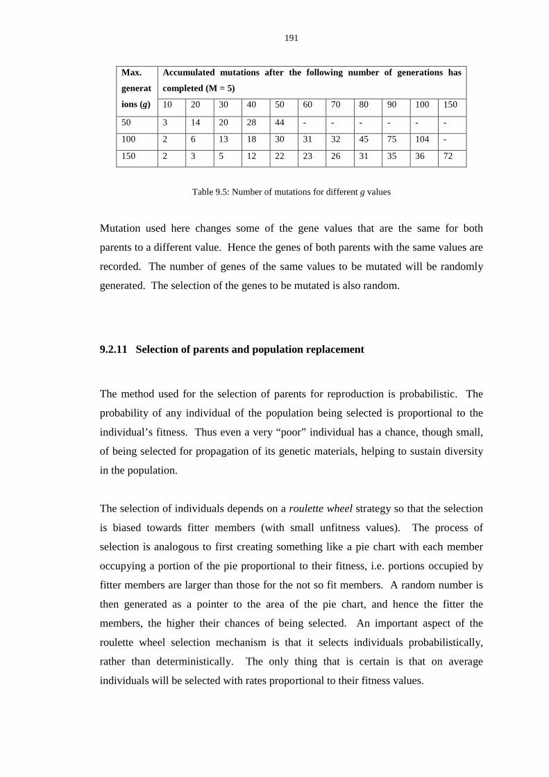
191
Accumulated mutations after the following number of generations has
completed (M = 5)
Max.
generat
ions (g) 10 20 30 40 50 60 70 80 90 100 150
50 3 14 20 28 44 - - - - - -
100 2 6 13 18 30 31 32 45 75 104 -
150 2 3 5 12 22 23 26 31 35 36 72
Table 9.5: Number of mutations for different g values
Mutation used here changes some of the gene values that are the same for both
parents to a different value. Hence the genes of both parents with the same values are
recorded. The number of genes of the same values to be mutated will be randomly
generated. The selection of the genes to be mutated is also random.
9.2.11 Selection of parents and population replacement
The method used for the selection of parents for reproduction is probabilistic. The
probability of any individual of the population being selected is proportional to the
individual’s fitness. Thus even a very “poor” individual has a chance, though small,
of being selected for propagation of its genetic materials, helping to sustain diversity
in the population.
The selection of individuals depends on a roulette wheel strategy so that the selection
is biased towards fitter members (with small unfitness values). The process of
selection is analogous to first creating something like a pie chart with each member
occupying a portion of the pie proportional to their fitness, i.e. portions occupied by
fitter members are larger than those for the not so fit members. A random number is
then generated as a pointer to the area of the pie chart, and hence the fitter the
members, the higher their chances of being selected. An important aspect of the
roulette wheel selection mechanism is that it selects individuals probabilistically,
rather than deterministically. The only thing that is certain is that on average
individuals will be selected with rates proportional to their fitness values.

192
The number of crossovers per generation has been arbitraril y set to be half the
population size. Offspring are separated from the current population so that they will
not be chosen for reproduction in the current generation. Since each mating produces
two offspring, at the end of a generation the maximum number of individuals would
be upto twice the population size when the generation started. The selection process
will also make sure that each crossover is between two different individuals.
9.2.12 Eliminating duplicates and population replacement
After a crossover, any new offspring whose chromosome is identical to that of an
already existing individual in the newly formed population member will be discarded.
A new offspring will also be discarded if after the construction operator has been
applied, its solution schedule is identical to that of an already existing member of the
new population. A new offspring will be added to the new population.
At the beginning of each generation a fixed size, n, population is maintained. In the
first generation, the entire population is created at random. After a generation has
completed, both the parent population and the children population are combined and
ranked according to their unfitness. The process of selecting the best members to
survive is deterministic. Only a certain number of the fittest individuals from the
merged population will ‘survive’ and be brought forward to the next generation. The
maximum number of individuals to survive is a fixed percentage, s, of a population
size (the parameter, s, is called the survival rate). The other individuals will be
discarded. New individuals are then created randomly to bring the total population
size back to n before the next generation of reproduction starts again.
There is no conclusive theory in deciding the best population size. Small population
sizes may have the danger of not covering the solution space satisfactorily.
Experience from various experiments indicates that, in general, the population size
should be proportional to the size of the problem. The size of a problem is measured
principally by the total number of work pieces, but it is also dependent on the total
number of potential shifts. However, our experiments have shown that by using
aggressive mutation, a significantly smaller population size would be adequate. In
our experiments, population sizes ranging from 50 to 500 have been used and 100
193
seems to be an adequate size for small to medium size problems (less than 100 shifts
in the schedule).
9.2.13 Termination criteria
The GA stops if one of the following conditions is satisfied:
1. A specified number of generations has been reached
2. The fittest member has survived a specified number (100 in our GA) of times
(convergence reached).
9.3 System parameters
It is desirable to parameterise some key values used by the GA so that various
experiments can be tried out efficiently. The performance of the GA can be fine
tuned by adjusting these parameters. There are two competing goals when setting
these system parameters in a GA run: the need for ‘selective pressure’ so that the GA
is able to focus the search on promising areas of the search space, and the need for
‘population diversity’ so that important information is not lost. The following
parameters are used to ‘tune’ the genetic search and these affect both selective
pressure and population diversity.
• Population size
In theory, the initial population should be big enough so that the solution space is
adequately covered. However, a large population will inevitably increase the
computational costs exponentially. The most often used value is 100 for problems
whose schedules have under 100 shifts. However, if the problem size is large, it is
found that higher values are needed to ensure population diversity. A large
population will inevitably increase the running time.
194
• Number of generations
This is one of the terminating criteria of the GA process and almost all the tests
carried out terminate because the required number of generations has been reached.
The most often used value is 100. The GA tends to converge very quickly and
sometimes a smaller value can be used for small problems (schedules with 50 or less
shifts).
• Minimu m fractional value for the preferred shifts
This parameter is for selecting a subset of preferred shifts which are considered to be
beneficial in forming a good schedule. This has the effect of narrowing down the GA
search to a small but promising solution space. Each selected preferred shift will be
represented by a gene in the chromosome. Values of 0.2 or 0.3 are often used as they
tend to give the best results.
• Survival rate
The survival rate is usually set to between 30% to 50% so that a significant number of
new species are added to the evolution process to ensure population diversity. The
most often used rate is 50%.
• Option to ban shifts
This optional feature reduces the number of input potential shifts to be considered by
the construction operator of the GA. Since the similar reduction heuristic used in the
ILP process is proven to be effective and successful in TRACS II , it is used in most
experiments except when the problem size is small. Using this feature will put strong
selective pressure on the GA process so that it may quickly focus the search on the
best individuals.

195
• Mutation control param eter
Mutation is an optional feature here. If it is required, the mutation control parameter,
M (≥ 1), is used to control the mutation rate. The higher the value M, the slower the
mutation rate will be. Mutation rate also directly depends on the number of
generations. If the number of generations is large, mutations will be slow at the
beginning and the rate will increase slowly but gradually throughout the process.
While the population size does not affect the mutation rate, a large population size
will ensure a good diversity of population members and hence there is no need to
have frequent mutation. In our experiments, M is set to between 1 and 5 for problems
with population size of 100 or smaller to ensure a gradual mutation rate. Some
problems with large population size have M being set to 10 to 20 so that mutations are
not so frequent.
For each individual test problem, the values of the above parameters may vary and
some trial and error is needed so that the best results can be achieved. It is a
balancing act of maintaining both population diversity and selective pressure.
Varying some of the parameters may put strong selective pressure on the GA at the
expense of population diversity, and the lack of diversity can lead the GA to
prematurely converge on a sub-optimal solution. Varying other parameters may relax
the selective pressure and maintain a high diversity, but the search may fail to
improve solutions.
9.4 Computational results
Since the GA being researched is designed to replace the branch and bound process of
TRACS II , which sometimes fails to find an integer solution, the experiments were
designed to run the GA process after the relaxed LP process has finished. The results
obtained by the GA process are then compared with the ones produced by allowing
the branch and bound process to complete. The problems used here are all real
instances and are generally larger than previous experiments carried out in our group
prior to this research and probably elsewhere. The reason of using large real
problems is to enable us to give a fair assessment on the GA performance and its
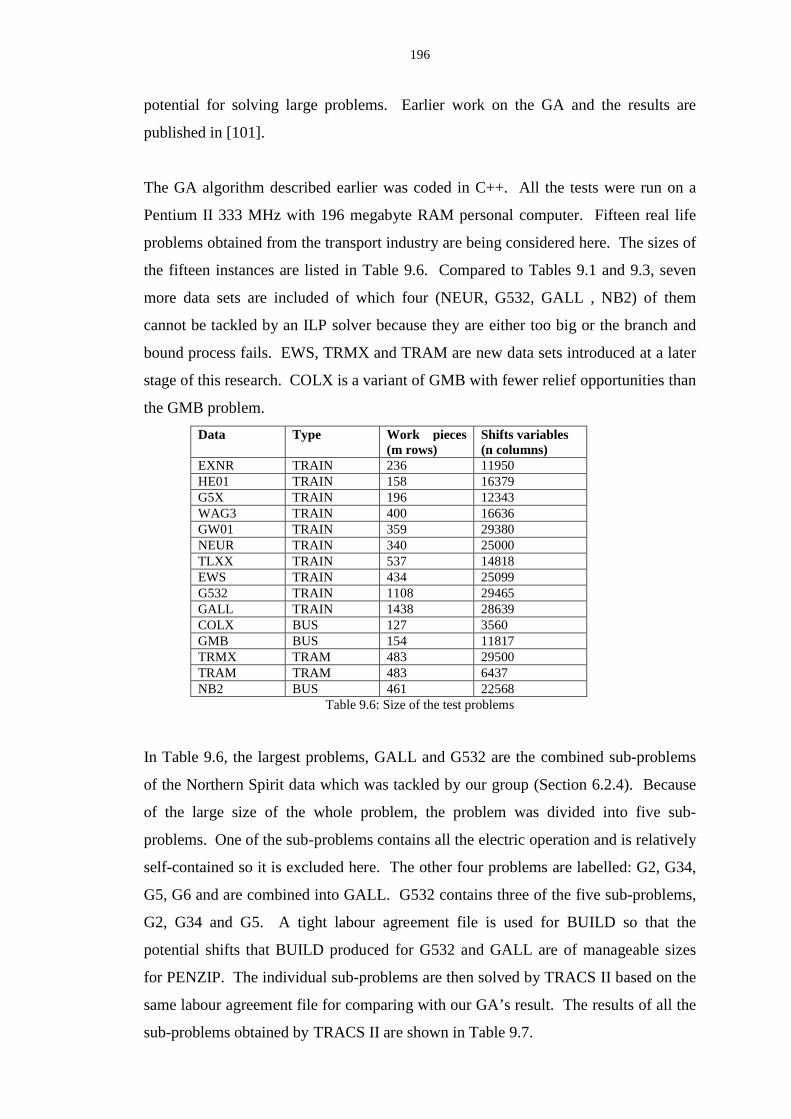
196
potential for solving large problems. Earlier work on the GA and the results are
published in [101].
The GA algorithm described earlier was coded in C++. All the tests were run on a
Pentium II 333 MHz with 196 megabyte RAM personal computer. Fifteen real life
problems obtained from the transport industry are being considered here. The sizes of
the fifteen instances are listed in Table 9.6. Compared to Tables 9.1 and 9.3, seven
more data sets are included of which four (NEUR, G532, GALL , NB2) of them
cannot be tackled by an ILP solver because they are either too big or the branch and
bound process fails. EWS, TRMX and TRAM are new data sets introduced at a later
stage of this research. COLX is a variant of GMB with fewer relief opportunities than
the GMB problem.
Data Type Work pieces(m rows)
Shifts variables(n columns)
EXNR TRAIN 236 11950HE01 TRAIN 158 16379G5X TRAIN 196 12343WAG3 TRAIN 400 16636GW01 TRAIN 359 29380NEUR TRAIN 340 25000TLXX TRAIN 537 14818EWS TRAIN 434 25099G532 TRAIN 1108 29465GALL TRAIN 1438 28639COLX BUS 127 3560GMB BUS 154 11817TRMX TRAM 483 29500TRAM TRAM 483 6437NB2 BUS 461 22568
Table 9.6: Size of the test problems
In Table 9.6, the largest problems, GALL and G532 are the combined sub-problems
of the Northern Spirit data which was tackled by our group (Section 6.2.4). Because
of the large size of the whole problem, the problem was divided into five sub-
problems. One of the sub-problems contains all the electric operation and is relatively
self-contained so it is excluded here. The other four problems are labelled: G2, G34,
G5, G6 and are combined into GALL. G532 contains three of the five sub-problems,
G2, G34 and G5. A tight labour agreement file is used for BUILD so that the
potential shifts that BUILD produced for G532 and GALL are of manageable sizes
for PENZIP. The individual sub-problems are then solved by TRACS II based on the
same labour agreement file for comparing with our GA’s result. The results of all the
sub-problems obtained by TRACS II are shown in Table 9.7.
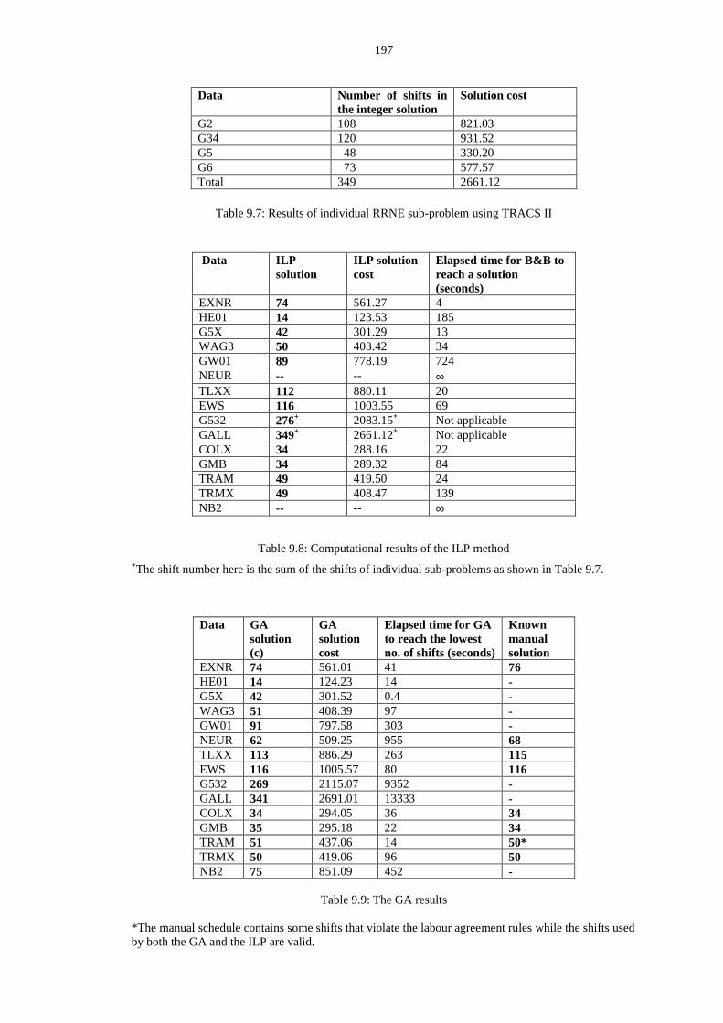
197
Data Number of shifts inthe integer solution
Solution cost
G2 108 821.03G34 120 931.52G5 48 330.20G6 73 577.57Total 349 2661.12
Table 9.7: Results of individual RRNE sub-problem using TRACS II
Data ILPsolution
ILP solutioncost
Elapsed time for B&B toreach a solution(seconds)
EXNR 74 561.27 4HE01 14 123.53 185G5X 42 301.29 13WAG3 50 403.42 34GW01 89 778.19 724NEUR -- -- ∞TLXX 112 880.11 20EWS 116 1003.55 69G532 276+ 2083.15+ Not applicableGALL 349+ 2661.12+ Not applicableCOLX 34 288.16 22GMB 34 289.32 84TRAM 49 419.50 24TRMX 49 408.47 139NB2 -- -- ∞
Table 9.8: Computational results of the ILP method+The shift number here is the sum of the shifts of individual sub-problems as shown in Table 9.7.
Data GAsolution(c)
GAsolutioncost
Elapsed time for GAto reach the lowestno. of shifts (seconds)
Knownmanualsolution
EXNR 74 561.01 41 76HE01 14 124.23 14 -G5X 42 301.52 0.4 -WAG3 51 408.39 97 -GW01 91 797.58 303 -NEUR 62 509.25 955 68TLXX 113 886.29 263 115EWS 116 1005.57 80 116G532 269 2115.07 9352 -GALL 341 2691.01 13333 -COLX 34 294.05 36 34GMB 35 295.18 22 34TRAM 51 437.06 14 50*TRMX 50 419.06 96 50NB2 75 851.09 452 -
Table 9.9: The GA results
*The manual schedule contains some shifts that violate the labour agreement rules while the shifts usedby both the GA and the ILP are valid.
198
In Table 9.8 we present the results obtained by the ILP method. The results for G532
and GALL are the sum of the solutions of the sub-problems. In two instances, NEUR
and NB2, the ILP process fails to obtain any integer solution even though the ILP
process has been re-run many times and each time with a higher revised target number
of shifts. Unless indicated otherwise, the elapsed time taken to obtain the result
shown here is only for the branch and bound run to obtain the first integer solution
(the time taken in the primal phase prior to the branch and bound phase is excluded
for fair comparison). In instances EWS, G532, GALL several ILP runs were needed
because the branch and bound process failed to find any integer solution with the
target suggested by the relaxed solution. The target number of shifts had to be raised
and in some of these runs, the branch and bound terminated after 500 nodes. The time
required in each such failed case varies from less than half an hour (EWS) to about
two hours for GALL. In GALL, ten ILP runs (each with a different number of shifts
target) were needed for one of the sub-problems before an integer solution was found
and the total elapsed time is more than one day.
The results obtained by the GA process are presented in Table 9.9. For each test
problem, several runs were needed for tuning the parameters in order to get the best
results. In cases when the ILP solver is unable to yield an integer solution, the target
number of shifts indicated by the relaxed LP solution is used as a guideline as to how
good the GA solutions are. The parameters that required frequent tuning are: number
of generations, the M value for mutation, the minimum fractional value of the
preferred shifts and the survival percentage. One encouraging result is that all except
two (GMB and TRAM) of the solutions obtained by the GA method have smaller or
equal number of shifts compared with the known manual solutions. For TRAM, the
manual schedule contains shifts that violate the labour agreement file.
Of the fifteen test data sets, five of the GA results equal to those produced by the ILP
method in terms of number of shifts. Four of these five problems are train problems.
For G532 and GALL, GA’s solutions are better than the combined ILP solutions in
terms of number of shifts. The cost of G532 obtained by ILP is better than the GA’s
result. In GALL and G532, if the labour agreement is relaxed and a good problem
decomposition strategy is used, the number of shifts should be further reduced by
using an ILP.
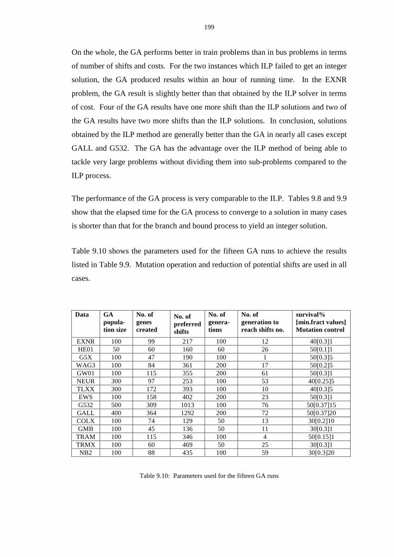
199
On the whole, the GA performs better in train problems than in bus problems in terms
of number of shifts and costs. For the two instances which ILP failed to get an integer
solution, the GA produced results within an hour of running time. In the EXNR
problem, the GA result is slightly better than that obtained by the ILP solver in terms
of cost. Four of the GA results have one more shift than the ILP solutions and two of
the GA results have two more shifts than the ILP solutions. In conclusion, solutions
obtained by the ILP method are generally better than the GA in nearly all cases except
GALL and G532. The GA has the advantage over the ILP method of being able to
tackle very large problems without dividing them into sub-problems compared to the
ILP process.
The performance of the GA process is very comparable to the ILP. Tables 9.8 and 9.9
show that the elapsed time for the GA process to converge to a solution in many cases
is shorter than that for the branch and bound process to yield an integer solution.
Table 9.10 shows the parameters used for the fifteen GA runs to achieve the results
listed in Table 9.9. Mutation operation and reduction of potential shifts are used in all
cases.
Data GApopula-tion size
No. ofgenescreated
No. ofpreferredshifts
No. ofgenera-tions
No. ofgeneration toreach shifts no.
survival%[min.fract values]Mut ation control
EXNR 100 99 217 100 12 40[0.3]1HE01 50 60 160 60 26 50[0.1]1G5X 100 47 190 100 1 50[0.3]5
WAG3 100 84 361 200 17 50[0.2]5GW01 100 115 355 200 61 50[0.3]1NEUR 300 97 253 100 53 40[0.25]5TLXX 300 172 393 100 10 40[0.3]5EWS 100 158 402 200 23 50[0.3]1G532 500 309 1013 100 76 50[0.37]15GALL 400 364 1292 200 72 50[0.37]20COLX 100 74 129 50 13 30[0.2]10GMB 100 45 136 50 11 30[0.3]1
TRAM 100 115 346 100 4 50[0.15]1TRMX 100 60 469 50 25 30[0.3]1NB2 100 88 435 100 59 30[0.3]20
Table 9.10: Parameters used for the fifteen GA runs
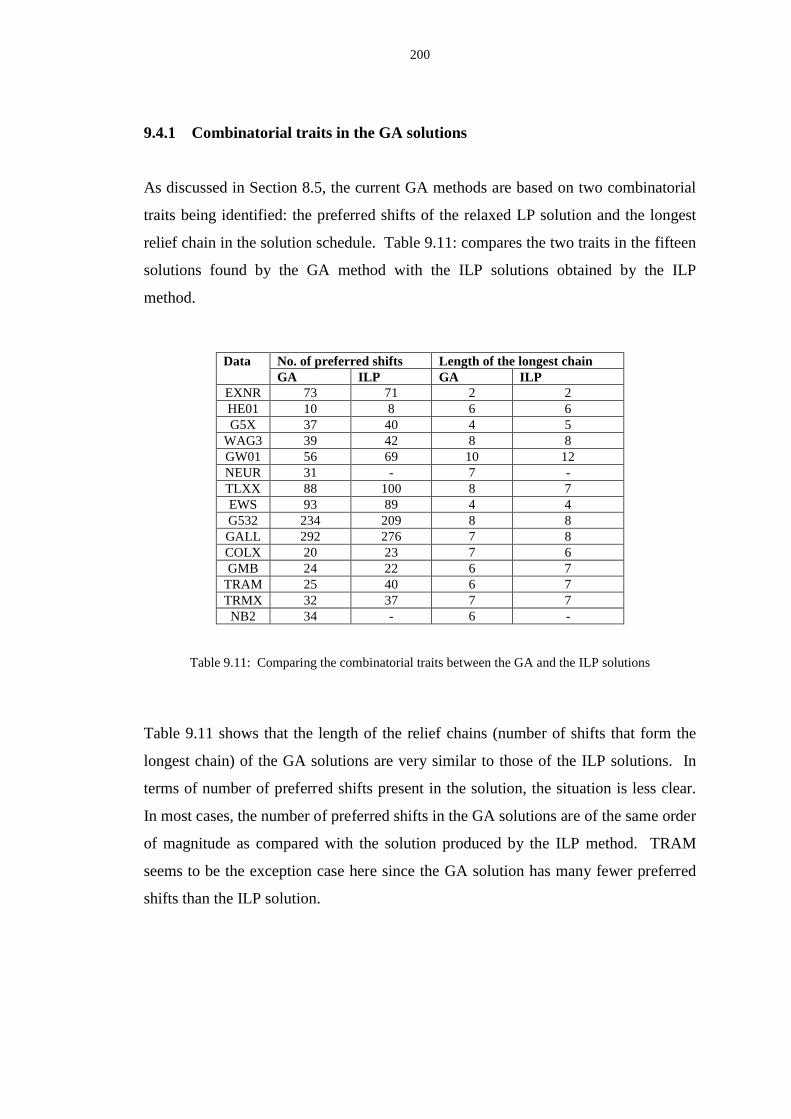
200
9.4.1 Combinatorial traits in the GA solutions
As discussed in Section 8.5, the current GA methods are based on two combinatorial
traits being identified: the preferred shifts of the relaxed LP solution and the longest
relief chain in the solution schedule. Table 9.11: compares the two traits in the fifteen
solutions found by the GA method with the ILP solutions obtained by the ILP
method.
No. of preferred shifts Length of the longest chainDataGA ILP GA ILP
EXNR 73 71 2 2HE01 10 8 6 6G5X 37 40 4 5
WAG3 39 42 8 8GW01 56 69 10 12NEUR 31 - 7 -TLXX 88 100 8 7EWS 93 89 4 4G532 234 209 8 8GALL 292 276 7 8COLX 20 23 7 6GMB 24 22 6 7
TRAM 25 40 6 7TRMX 32 37 7 7NB2 34 - 6 -
Table 9.11: Comparing the combinatorial traits between the GA and the ILP solutions
Table 9.11 shows that the length of the relief chains (number of shifts that form the
longest chain) of the GA solutions are very similar to those of the ILP solutions. In
terms of number of preferred shifts present in the solution, the situation is less clear.
In most cases, the number of preferred shifts in the GA solutions are of the same order
of magnitude as compared with the solution produced by the ILP method. TRAM
seems to be the exception case here since the GA solution has many fewer preferred
shifts than the ILP solution.
201
9.4.2 Using an alternative method to obtain a list of preferred shifts
Instead of using the relaxed LP method to obtain a list of preferred shifts, an
alternative method has been used to extract a list of shifts as ‘preferred shifts’ to input
to the GA process. The method used for the shifts extraction is SIEVE (see Section
5.8.1) which is one of the modules of TRACS II . SIEVE is the process that follows
the shift generation process BUILD and the function of SIEVE is to discard duplicate
shifts and, if necessary, eliminate those whose work was covered by many other
shifts. In removing the heavily covered shifts, the process works under the principle
that shifts whose work components are heavily covered by other shifts are deemed to
be of less importance.
Briefly, each potential shift is ranked using a combination of three attributes: an index
formulated to reflect its cost effectiveness (a status value), a least number (lowest
coverage) and an average number of other shifts (average coverage) covering the
individual pieces of work making up the shift. The lowest ranked shifts are discarded
in batches and the latter two attributes which affect the rankings are updated
continuously, until a pre-specified target number of shifts remain. The process is
modified so that the information required by the GA method is output and the version
is called SIEVE1. Two variants of SIEVE are also produced here and each version
uses a slightly different way to compute the ‘average coverage’ of the individual work
pieces. Since the criterion on ‘average coverage’ is different, the three processes will
produce three different sets of remained shifts. The ‘average coverage’ calculated in
the three processes are:
• SIEVE1: average number of shifts covering the individual work pieces of a shift
for all the spells.
• SIEVE2: average number of shifts covering the pieces in the spell containing the
lowest coverage for the shift
• SIEVE3: the average number of shifts covering the least covered work piece in
each spell
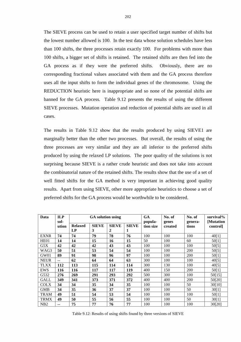
202
The SIEVE process can be used to retain a user specified target number of shifts but
the lowest number allowed is 100. In the test data whose solution schedules have less
than 100 shifts, the three processes retain exactly 100. For problems with more than
100 shifts, a bigger set of shifts is retained. The retained shifts are then fed into the
GA process as if they were the preferred shifts. Obviously, there are no
corresponding fractional values associated with them and the GA process therefore
uses all the input shifts to form the individual genes of the chromosome. Using the
REDUCTION heuristic here is inappropriate and so none of the potential shifts are
banned for the GA process. Table 9.12 presents the results of using the different
SIEVE processes. Mutation operation and reduction of potential shifts are used in all
cases.
The results in Table 9.12 show that the results produced by using SIEVE1 are
marginally better than the other two processes. But overall, the results of using the
three processes are very similar and they are all inferior to the preferred shifts
produced by using the relaxed LP solutions. The poor quality of the solutions is not
surprising because SIEVE is a rather crude heuristic and does not take into account
the combinatorial nature of the retained shifts. The results show that the use of a set of
well fitted shifts for the GA method is very important in achieving good quality
results. Apart from using SIEVE, other more appropriate heuristics to choose a set of
preferred shifts for the GA process would be worthwhile to be considered.
GA solution usingData ILPsol-ution Relaxed
LPSIEVE3
SIEVE2
SIEVE1
GApopula-tion size
No. ofgenescreated
No. ofgenera-tions
survival%[Mutationcontrol]
EXNR 74 74 79 78 76 100 100 100 40[1]HE01 14 14 15 16 15 50 100 60 50[1]G5X 42 42 42 43 43 100 100 100 50[5]WAG3 50 51 53 54 54 100 100 200 50[5]GW01 89 91 98 96 97 100 100 200 50[1]NEUR -- 62 64 64 63 300 100 100 40[5]TLXX 112 113 115 114 114 300 130 100 40[5]EWS 116 116 117 117 119 400 150 200 50[1]G532 276 269 291 293 292 500 300 100 50[15]GALL 349 341 373 371 372 400 400 200 50[20]COLX 34 34 35 34 35 100 100 50 30[10]GMB 34 35 36 37 37 100 100 50 30[1]TRAM 49 51 54 53 54 100 100 100 50[1]TRMX 49 50 55 56 55 100 100 50 30[1]NB2 -- 75 77 76 77 100 100 100 30[20]
Table 9.12: Results of using shift s found by three versions of SIEVE
203
9.5 Conclusions
1. TRACS II uses an ILP based technique for the shift selection using the set-
covering formulation. It has been successful in solving many real life problems.
However, the ILP process in some cases has difficulties finding an integer
solution. Also, there exists the need for improvement in terms of computational
efficiency and capacity of solving large-scale instances. This situation motivated
us to propose a GA method to tackle the computational difficulties.
2. The earlier GA work in solving the driver scheduling problem in our group
produced schedules typically within a few duties of the results obtained by the ILP
method. One of the reasons was that the GA of previous work often started on a
very large search space. There was no initial reduction in the search space and the
GA often converged prematurely to a sub-optimal solution except in very small
problems.
3. The GA method uses specific problem knowledge and narrows the initial search to
a promising solution space. The knowledge which has been exploited is the list of
shifts making up the relaxed LP solution before the branch and bound phase of the
ILP method. Another feature of our GA method is to introduce inheritance of the
longest relief chain from the parents to the children. These innovative features are
specific to the structure of the driver scheduling problems and are able to guide
the search efficiently.
4. We use a binary string of genes to represent the chromosome. These genes do not
represent a solution schedule on their own. Instead, they are used as the ‘building
blocks’ of a solution. The construction operator makes use of these ‘building
blocks’ and the inherited relief chain shifts to construct a solution. The heuristic
takes a greedy approach and it has been able to find good solution efficiently.
5. Since the binary string representation is used here, simple single point crossover
can be used. It has the advantage of being able to maintain useful bit patterns
together after crossover and the quality of solution is thus maintained.
204
6. We use an effective technique for reducing the number of potential shifts for the
GA search and this is found to be very beneficial in enhancing the quality of the
solution and the computational performance.
7. The mutation rate is variable and adaptive. The mutation rate is dependent on the
longevity of the best member as well as the total number of generations of the GA.
This has been found to be useful in introducing diversity to the population
especially when such a need is the greatest when the GA starts to converge. The
mutation rate used in our experiments is usually high in order to introduce varied
members to the population. Although a high mutation rate may disrupt important
gene patterns, our GA method only mutates the children and keeps the parents’
chromosomes intact and the best of the combined population are carried forward
to the next generation.
8. The GA method has been used to solve real life problems and some of them are
very large (the largest set has 1438 rows). Our computational testing showed that
the GA leads to good results and some of them are as good as the solutions found
by the ILP method.
9. In two of the instances when the ILP method failed to find any integer solution,
the GA process can reach a good solution. The GA results are better than or equal
to the known manual schedules in terms of number of shifts.
10. The GA method works better on train driver problems than on bus driver
problems. An explanation is that train driver problems usually involve a certain
amount of overcover (slackness) in the solution and hence the corresponding
solution space is wider than the bus problems whose solution usually have very
little slackness.
11. Another encouraging finding is that the performance of the GA was very similar
or even faster than the branch and bound process of the ILP.
12. Experiments have been carried out using other ways to select a set of ‘preferred
shifts’ for the GA process. This produced inferior results with solutions having a

205
few more shifts than the GA solutions using the preferred shifts from the ILP.
This demonstrated that having a set of well fitted shifts as preferred shifts is very
important in achieving good quality results.
13. There are several limitations of the GA method used here. The fitness function
used here only puts pressure on minimising the number of shifts and then
minimising the total costs. The function may also be too simplistic because it
gives no indication of the combinatorial characteristics of the schedule. An area
in which the fitness function might be improved is suggested in Section 9.6.
14. The GA relies heavily on the construction operator which is deterministic in
nature. This might have made it diffi cult for the GA to get out of local optima.
The author did introduce randomness in the construction process but the results
were worse than those obtained by the deterministic approach. Another way that
could improve the quality of the GA solution is to use a local search technique.
This can be applied to the solution obtained immediately after each construction
process or at the very end of the GA process after it converges.
In conclusion, we demonstrated that our GA method could solve real-world driver
scheduling problems of all sizes with good results and performance in many cases
compared to the ILP method. Most importantly, there are cases when the ILP fails to
find any integer solution whereas the GA can find solutions (one of them is even
better than the manual solution). The GA will always gives an integer solution at any
stage of the process whereas the ILP has to be run to completion and it does not
always guarantee to yield an integer solution at all. Also, in some large instances, the
ILP requires problem decomposition in order to cope whereas our GA does not
require decomposition and the results obtained by the GA have fewer shifts compared
to the sum of the shifts of individual sub-problems solved by the ILP.
9.6 Future work
There are a number of interesting areas for future research in the GA method. These
include enhancements in the algorithm, improvements in the performance and
exploring the possibility of hybridising GA with other metaheuristics.
206
9.6.1 Escaping from a local optimum
Similar to most of the GA work in combinatorial optimisation problems, one of the
main limitations is that it can converge prematurely to a sub-optimal solution. The
running of the GA on the test data shows that most of the progress made by GA
occurs early in the search. In all the cases, the GA converges to a final solution
within 80 generations. The use of a larger population size and a more intensive
mutation rate have little effect on diversifying the search at a latter stage of the
process. This suggests that once the GA process starts to converge, even when a very
strong diversity force is applied, it is difficult for the GA process to escape from a
local optimum. The following are a few suggestions for maintaining diversity and
forcing the GA to search ‘unvisited’ regions:
1. After the GA process starts to converge, the GA process can be ‘r e-started’ from
the beginning using a larger set of preferred shifts. For example, the process may
start with a set of preferred shifts whose fractional value is equal to or above 0.3.
If the GA process is re-started, a set of preferred shifts with lower fractional value,
say 0.05, can be used. Obviously, the best individuals in the previous run are to
be kept in the population.
2. Another approach is to generate different independent populations and each one
has its own GA process operating in parallel while occasionally allowing fit
members to migrate between the populations [94]. This can be implemented, for
example, on a computer capable of parallel processing.
3. Another approach is hybridising a local search technique with the construction
operator. After an initial solution has been found, the local search technique can
be used to improve the solution. The local search can be a simple exchange of
work pieces or shift variables so that a neighbourhood is formed. This has the
obvious disadvantage of increasing the computational time of the GA. However,
our GA process has the advantage that it performs very fast even for very large
problems, an improvement in the quality of solution can be considered as a
sensible trade-off to computing cost.

207
4. It may be worthwhile to build some memory structure into the generation of
population members like tabu search so that it can prevent the GA from
generating the same member repetitively for a number of iterations.
9.6.2 Other possible traits
Although the following two possible traits have been investigated, they have not been
implemented in this research. The main reason why they are not implemented is that
they might have made the GA process over-complex. However, they may have
significance in assisting the GA to search for an optimal solution, and they are
possible areas for future research.
1. Handover opportunities
When a shift finishes on a vehicle which still has work to be covered, the
relieving driver may be either starting a new shift or resuming work after a
break. In the former case, the relief opportunity used is called handover
opportunity. In the latter case, the relief opportunity terminates a relief chain as
described earlier.
Some handover opportunities used in the solution schedules might be critical to
the formation of good schedules. When this information is passed on to an
offspring, handover opportunities could be used by the construction operator to
give priority to selecting shifts covering the work pieces adjacent to the
handover opportunities. Shifts covering both work pieces adjacent to a
handover opportunity, i.e. not using it to relieve another driver, would be
banned.
2. Overcover Link
One phenomenon in this area of research is that a GA may converge
prematurely to a solution using more shifts than the minimum suggested by the
relaxed solution. Since more shifts than the minimum are used, some overcover
is expected. It is interesting that although they are inefficient, the pieces of
overcover have persisted in the evolutionary process. One explanation could be
208
that there is something critical with one or more pieces of work linked to the
overcovered piece, and the GA has not been able to yield an optimal
combination of shifts to accommodate the critical feature. It is likely that only
one of the pair of shifts involved in an overcover is obstructing the formation of
an optimal combination of shifts, and it might be possible to avoid the linkages
leading to the overcover. However, the remedy would need more reformation
or backtracking than simply replacing the shift at fault. What could be done is
for the subsequent evolutionary steps to enforce the critical features identified
and to ban the linkages suspected to be at fault.
9.6.3 Other areas
There are other issues that can be investigated in future work:
1. A more sophisticated fitness or unfitness function may be needed to reflect the
combinatorial fitness of the solution. This may include the use of penalty weights
to penalise undesirable features in the schedules such as too many three or four
spells shifts. However, a ‘bad’ driver schedule may contain good features which
would be desirable to be carried forward to the next generations.
2. The GA method used here passes the longest relief chain from one of the parents
to one of the children. This is to ensure a ‘good trait’ is present in the children’s
solution schedule. A different variation to this can be tried. For example, both
sets of relief chains can be passed to a child, or the crossover can produce eight
children instead of two (and only the best two are kept) and each will inherit from
the parents in different ways. However, a balance must be maintained so that the
children’s solution schedules should not be pre-dominated by the presence of the
parents’ solution shifts.
3. Choice of chromosome structure is very important in a GA. Our GA uses a binary
string to represent part of the solution which forms the basic building block of the
whole schedule. Possible structures include representing pieces of work sorted in
chronological order as genes in the chromosome. A subset of the preferred shifts
209
are then selected randomly from the list of preferred shifts to cover the work
pieces. This would allow a single-point crossover to take place at a particular
time of day and would assist the combination of a good morning schedule with a
good afternoon schedule. A slight variation from our present chromosome
structure is to make the order of shifts in the chromosome significant by, say,
arranging each shift to occupy a particular gene position if it shares a relief
opportunity with its predecessor.
4. A different type of mutation to augment the present mutation may be needed to
introduce a more substantial change in the gene pattern than the present way of
changing the bit values of the chromosome. One possibility is to re-shuffle the
gene ordering of the chromosome randomly at infrequent intervals. Obviously,
the best population members are stored before this happens. Although this may
disrupt important schemata in the offspring, this has the advantages of introducing
new search region to the GA and helping it to escape from a local optimum.
5. Finally, the present work on GA shows that using the preferred shifts of the
solution to the LP relaxation to initiate the GA produces good results. We also
demonstrated randomly selecting a set of shifts (e.g by the process SIEVE) to
initiate the GA process will lead to inferior results. Further work can be done on
using heuristics for finding a set of well fitted shifts as a replacement of the LP
relaxation process completely. By combining the heuristic with our GA method,
the entire mathematical programming process for shift selection might then be
replaced.
210
Chapter Ten
Conclusions
10.1 Summary
The theme of this research is to tackle the train driver scheduling problem in the U.K.
Train driver scheduling problems are highly constrained and are far more complex
than most bus problems. The complexity of the problem is described in Chapter One.
A review of methods and systems for train driver scheduling is presented in Chapter
Two. Since the bus driver scheduling problem has some similarities to train driver
scheduling, reviews on solving the bus driver scheduling problems are also presented.
The high-level solution framework used by a successful bus driver scheduling system,
IMPACS, has been adopted in this research. The method is based on set covering and
involves two stages. The first stage is the generation of a large set of feasible
potential shifts and the second stage is the selection of a subset of shifts to cover all
the work at minimum cost.
Two tasks are identified for this research and ordered by their priority. They are as
follows:

211
1. To develop solution strategies and a generic method for creating legal and
operable shifts meeting nearly all of the present constraints for the train operation,
and easily extensible to meet future requirements
2. To explore of the use of Genetic Algorithms as an alternative to the mathematical
approach for shift selection
The result of this research for task one above is a new method of shift generation
meeting nearly all of the operational constraints of the problem. The new process of
shift generation is combined with an ILP solver, which is much improved from that
used by IMPACS to produce schedules. The new system is called TRACS II and an
overview of the system is presented in Chapter Three.
Chapter Four and Chapter Five discuss the main methods used in tackling task one.
Chapter Four discusses the problem of specifying passenger travel trips used by the
drivers which is one of the most important features in the train problem. Chapter
Five describes a new shift generation method which has incorporated nearly all
(except Windows of relief opportunities) the requirements identified in Chapter One.
The new shift generation method, BUILD, which is driven by parameters describing
the labour agreement rules, produces a variety of legal and operable shifts. The
BUILD process incorporates some heuristics so that shifts that are unlikely to be
useful to form a good schedule are eliminated. TRACS II have been tested on a
variety of train and bus problems and the schedules produced are not only operable
but are more efficient compared with the existing manual schedules (Chapter Six).
Occasionally, there are inherent computational difficulties in the ILP process. The
branch and bound process may fail to find any integer solution (Chapter Seven) and it
can be time-wasting and frustrating. The second task of the research is to investigate
the use of GA for the shift selection process as a possible alternative to the ILP
process. Owing to the very large search space, a GA method with specific domain
knowledge is proposed. In order to obtain good results, a substantial reduction of the
search space is required. The GA makes use of the information provided by the
relaxed LP solution of the ILP process in the construction of the chromosome. It also
212
uses a reduction heuristic to eliminate some potential shifts from being considered by
the schedule construction operator (Chapter Eight).
The GA method proposed is implemented and it has been tested on a number of real
life train and bus problems. The GA method produces good results, half of which
have the same number of shifts as those found by the ILP process (Chapter Nine).
Various directions for improving the GA method are suggested in Chapter Nine.
10.2 Future work on train driver scheduling
There are a number of interesting areas for future research in train driver scheduling
problems. Further research that follows the GA work has already been discussed in
Chapter Nine.
• Windows of relief opportunities
When a train stops at a location, there is often a gap between the arrival time and the
departure time and often a driver is required to cover this time gap. In practice, the
driver on that train may be relieved at any time during this time gap which is known
as a ‘window of relief opportunities’. However, the present BUILD cannot cope with
windows of relief opportunities because it requires relief opportunities to be discrete
not continuous. Windows can be transformed into discrete timing points if every
minute within the time gaps is represented as individual relief opportunities. Clearly
this is not practicable because it will create an explosion in problem size. This will
also create problems for the ILP solver because some of the work pieces may be as
short as one minute. Train schedules usually contain a high proportion of windows
and they have to be simplified when they are transferred into TRACS II format.
Usually, only the arrival time of each window is used as a relief opportunity. If
TRACS II were offered the flexibility provided by windows, more efficient shifts
could have been created. For instance, the relieved driver on that train could have
been relieved a bit later than the train arrival time so that the relieving driver (one who
takes over the train from the relieved driver) could have made a more economical
passenger trip than before.
213
• Non-wheel turning tasks
In addition to train driving work, a driver may be responsible for a number of non-
wheel turning tasks, for example, train preparation, disposal, etc. There is no fixed
schedule as to when precisely these tasks should be performed, hence they are also
called ‘soft tasks’. For instance, a train may have to be ‘prepared’ any time before it
leaves the depot in the morning. However, BUILD only deals with scheduled work
and these soft tasks have to be time specific in the data. At present, these tasks are
attached before or after the driving work as required so that these tasks are essentially
fixed at a certain time. Hence the scheduling flexibilit y of these tasks is lost. Further
research is needed to derive methods to schedule such soft tasks most efficiently.
• Lodging
Sometimes, a driver may finish work at a place which is far from his/her home depot
and is required to lodge at that place. The same driver will have to come back to his
home depot the next day via a different shift. A shift with lodging will have different
start and end depots. The issue of lodging is complicated because it is also affected
by the rostering requirements. Also, the change of work day schedule, e.g. from
Friday schedule to Saturday schedule, adds more complexity to the problem. A driver
who lodges on Friday must take a compatible shift on Saturday in order to bring the
driver home, the same applies to Saturday, Sunday and Sunday to Monday. The issue
of lodging is similar to air crew pairing in which the time scale in question spans more
than one day. At present, BUILD will not create shifts that start and end at different
depots and only considers scheduling drivers in a single working day.
• Taking a mealbreak while travelling as passenger
At present, a mealbreak must take place at some location which is a fixed place. In
practice, some operators may require the drivers to have their meals while they are
travelling as passengers on a train. Not all trains taken by drivers for passenger travel
can provide proper facilities for having mealbreaks. Drivers taking mealbreaks while
travelling as passengers is clearly an efficient way of utilising resources. Further
work is therefore needed in order to cater for this feature.

214
• Formation of shifts with more than four spells
The maximum number of spells in a shift that BUILD creates is four. In many
manual schedules, shifts with more than four spells are not unusual. Although
TRACS II can produce better schedules than the manual ones even with this limit, we
cannot rule out the possibility that TRACS II could have produced even better
schedules had it been allowed to create shifts with more than four spells. Increasing
the number of spells in a shift will no doubt provide a greater variety of shifts but the
drawback is that it will increase the number of possible combinations exponentially.
Further research is therefore needed on how to control the formation of shifts with
more than four spells.
• Reduction in problem size by de-selecting some relief opportunities
Work on de-selecting relief opportunities has been carried out at Leeds for the bus
driver scheduling problem. However, there has been no similar research in the train
problem. De-selecting some relief opportunities in the train problems will benefit the
scheduling process a great deal because train problems are usually very big.
However, the presence of route knowledge, traction knowledge and multi-depot
would substantially complicate the process of de-selecting relief opportunities. Also,
it is important that critical relief opportunities are identified and not de-selected.
10.3 Achievements in this research
In conclusion, work on the first task in this research results has resulted in a new train
driver scheduling system TRACS II which has been developed to take account of the
conditions relating specially to the train situation. The TRACS II system combines
heuristics used in the shift generation stage with the mathematical process used in the
shift selection stage. TRACS II has been extensively tried and tested in the field for
many different train and bus situations. It is currently implemented in two bus
companies. Work on the second task in this research results in a new GA model
which makes use of the specific knowledge gained in the mathematical process as an
alternative for shift selection. The results produced by the new GA model in many

215
cases are as good as those obtained by TRACS II in terms of number of shifts and
performance. The GA will always gives an integer solution at any stage of the process
whereas the ILP has to be run to completion and it does not always guarantee to yield
an integer solution at all. The new GA model can be used in a fall-back position
should the ILP of TRACS II fails to find any integer solution. Also the GA model can
solve very large problem instances which, if solved by an ILP, would usually require
decomposition.
216
Bibliography
[1] M. E. Parker and B. M. Smith, Two Approaches to Computer Crew Scheduling,in: Proceedings of Second International Workshop on Computer-AidedScheduling of Public Transport, ed. A. Wren (North-Holland, 1991) pp. 193-221.
[2] B. M. Smith. Bus Crew Scheduling using Mathematical Programming. PhDthesis, University of Leeds, 1986.
[3] B. M. Smith and A. Wren, A Bus Crew Scheduling System Using a SetCovering Formulation. Transportation Research, 22A: 1988 pp. 97-108.
[4] A. Wren and B. M. Smith, Experiences With a Crew Scheduling System Basedon Set Covering, in: Proceedings of the Fourth International Workshop onComputer-Aided Scheduling of Public Transport, eds. J. R. Daduna and A. Wren(Springer-Verlag, 1988) pp. 104-118.
[5] B. M. Smith and M. E. Parker, University of Leeds IMPACS Crew-SchedulingSystem User Manual (Amdahl Version). University of Leeds, October 1993.
[6] M. E. Parker, A. Wren and R. S. K. Kwan, Modelling the Scheduling of TrainDrivers, in: Proceedings of the Sixth International Workshop on Computer-Aided Scheduling of Public Transport, eds. J. R. Daduna, I. Branco and J. M. P.Paixáo (Springer-Verlag, 1995) pp. 359-370.
[7] A. Wren, Private Communication (1992).
[8] W. P. Wil lers. Improved Algorithms for Bus Crew Scheduling. PhD thesis,University of Leeds, 1995.
[9] S. Fores. Column Generation Approaches to Bus Driver Scheduling. PhDthesis, University of Leeds, 1996.
[10] Preprints of the International Workshop on Automated Techniques forScheduling of Vehicle Operators for Urban Public Transportation Services,Chicago, 1975.
[11] A. Wren (ed.), Computer Scheduling of Public Transport, Proceedings of theSecond International Workshop on Computer-Aided Scheduling of PublicTransport (North-Holland, 1981).
[12] J.-M. Rousseau (ed.) Computer Scheduling of Public Transport 2, Proceedingsof the Third International Workshop on Computer-Aided Scheduling of PublicTransport (North-Holland, 1985).

217
[13] J. R. Daduna and A. Wren (eds.), Computer-Aided Transit Scheduling,Proceedings of the Fourth International Workshop on Computer-AidedScheduling of Public Transport (Springer-Verlag, 1988).
[14] M. Desrochers and J.-M. Rousseau (eds.), Computer-Aided Transit Scheduling,Proceedings of the Fifth International Workshop on Computer-Aided Schedulingof Public Transport (Springer-Verlag, 1992).
[15] J. R. Daduna, I. Branco and J. Paixáo (eds.), Computer-Aided TransitScheduling, Proceedings of the Sixth International Workshop on Computer-Aided Scheduling of Public Transport (Springer-Verlag, 1995).
[16] N. H. M. Wilson (ed.), Computer-Aided Transit Scheduling, Proceedings of theSeventh International Workshop on Computer-Aided Scheduling of PublicTransport (Springer-Verlag, 1999).
[17] J. A. Ellis and H. Savin, Crew Scheduling on Railways, with particularreferenece to the Local Area Problem. Presented at the 13th Annual Seminar onPublic Transport Operations Research, Univeristy of Leeds, 1981.
[18] R. J. Tykulsker, K. K. O’Neil, A. Ceder and Y. Sheffi, A Commuter Rail CrewAssignment/Work Rules Model, in: Proceedings of the Third InternationalWorkshop on Computer-Aided Scheduling of Public Transport, ed. J.-M.Rousseau (North-Holland, 1985) pp. 233-246.
[19] D. M. Ryan and B. A. Foster, An Integer Programming Approach to Scheduling,in: Proceedings of the Second International Workshop on Computer-AidedScheduling of Public Transport, ed. J.-M. Rousseau (North-Holland, 1981) pp.269-280.
[20] A. Caprara, M. Fischetti, P. L. Guida, P. Toth and D. Vigo, Solution of Large-Scale Railway Crew Planning Problems: the Italian Experience, in: Proceedingsof the Seventh International Workshop on Computer-Aided Scheduling of PublicTransport, ed. N. H. M . Wilson (Springer-Verlag, 1999) pp. 1-18.
[21] E. M. Morgado and J. P. Martins, CREW_NS: Scheduling Train Crew in TheNetherlands, in: Proceedings of Innovative Applications of Artificial IntelligenceConference: 9th : 1997 : Providence, Rhode Island, AAA I Press/MIT Press,1997 pp. 893-902.
[22] R. Bisiani, Beam Search, in: Encyclopedia of Artificial Intelligence, ed. S. C.Sapiro (New York: John Wiley and Sons, 1987) pp. 56-58.
[23] J. Hoffstadt, Computerised Vehicle and Driver Scheduling for the HamburgerHochbahn Aktiengesellschaft, in: Proceedings of the Second InternationalWorkshop on Computer-Aided Scheduling of Public Transport, ed. A. Wren(North-Holland, 1981) pp. 35-52.
[24] J. R. Daduna and M. Mojsilovic, Computer-Aided Vehicle and Duty SchedulingUsing the HOT Programme System, in: Proceedings of the Fourth InternationalWorkshop on Computer-Aided Scheduling of Public Transport, eds. J. R.Daduna and A. Wren (Springer-Verlag, 1988) pp. 133-146.

218
[25] M. Völker and P. Schütze, Recent Developments of the HOT System, in:Proceedings of the Sixth International Workshop on Computer-Aided Schedulingof Public Transport, eds. J. R. Daduna, I. Branco and J. M. P. Paixáo (Springer-Verlag, 1995) pp. 334-348.
[26] R. Lessard, J.-M. Rousseau and D. Dupuis, HASTUS I: A MathematicalProgramming Approach To The Bus Driver Scheduling Problem, in:Proceedings of the Second International Workshop on Computer-AidedScheduling of Public Transport, A. Wren (North-Holland, 1981) pp. 255-267.
[27] P. Carraresi and J.-M. Rousseau, Relaxation Approaches to Large Scale BusDriver Scheduling Problems, in: Transportation Research, 16B: 1982 pp. 383-397.
[28] J.-M. Rousseau and J.-Y. Blais, HASTUS: An Interative System for Buses andCrew Scheduling, in: Proceedings of the Third International Workshop onComputer-Aided Scheduling of Public Transport, ed. J.-M. Rousseau (North-Holland, 1985) pp. 45-60.
[29] J.-M. Rousseau, R. Lessard and J.-Y. Blais, Enhancements to the HASTUSCrew Scheduling Algorithm, in: Proceedings of the Third InternationalWorkshop on Computer-Aided Scheduling of Public Transport, ed. J.-M.Rousseau (North-Holland, 1985) pp. 295-310.
[30] J.-Y. Blais and J.-M. Rousseau, Overview of HASTUS Current and FutureVersions, in: Proceedings of the Fourth International Workshop on Computer-Aided Scheduling of Public Transport, eds. J. R. Daduna and A. Wren (Springer-Verlag, 1988) pp. 175-187.
[31] N. Hamer and L. Seguin, The HASTUS System: New Algorithms and Modulesfor the 90s, in: Proceedings of the Fifth International Workshop on Computer-Aided Scheduling of Public Transport, eds. M. Desrochers and J.-M. Rousseau(Springer-Verlag, 1992) pp. 17-29.
[32] V.J. Rayward-Smith, I. Osman, C.R. Reeves and G. D. Smith (eds), ModernHeuristic Search Methods (Wiley, 1996).
[33] A. Wren, B. M. Smith and A. J. Mil ler, Complementary Approaches to CrewScheduling, in: Proceedings of the Third International Workshop on Computer-Aided Scheduling of Public Transport, ed. J.-M. Rousseau (North-Holland,1985) pp. 263-278.
[34] M. Chamberlain and A. Wren: Developments and Recent Experience with theBUSMAN and BUSMAN II Systems, in: Proceedings of the Fifth InternationalWorkshop on Computer-Aided Scheduling of Public Transport, eds. M.Desrochers and J.-M. Rousseau (Springer-Verlag, 1992) pp. 1-15.
[35] L. K. Luedtke, RUCUS II: A Review of System Capabilities, in: Proceedings ofthe Third International Workshop on Computer-Aided Scheduling of PublicTransport, ed. J.-M. Rousseau (North-Holland, 1985) pp. 61-116.
219
[36] L. O. Ball, L. D. Bodin and J. Greenberg, Enhancements to the RUCUS 2 crewscheduling system, in: Proceedings of the Third International Workshop onComputer-Aided Scheduling of Public Transport, ed. J.-M. Rousseau (North-Holland, 1985) pp. 279-293.
[37] E. B. Wilhelm, Overview of the RUCUS Package Driver Run Cutting Program(RUNS), paper presented at the International Workshop on AutomatedTechniques for Scheduling of Vehicle Operators for Urban PublicTransportation Services, Chicago, 1975.
[38] M. Desrochers and F. Soumis, CREW-OPT: Crew Scheduling by ColumnGeneration, in: Proceedings of the Fourth International Workshop onComputer-Aided Scheduling of Public Transport, eds. J. R. Daduna and A. Wren(Springer-Verlag, 1988) pp. 83-90.
[39] M. Desrochers, J. Gilbert, M. Sauvé and F. Soumis: CREW-OPT: SubproblemModelling in a Column Generation Approach to Urban Crew Scheduling, in:Proceedings of the Fifth International Workshop on Computer-Aided Schedulingof Public Transport, eds. M. Desrochers and J.-M. Rousseau (Springer-Verlag,1992) pp. 395-406.
[40] J.-M. Rousseau and M. Desrochers, Results Obtained with Crew-Opt, a ColumnGeneration Method for Transit Crew Scheduling, in: Proceedings of the SixthInternational Workshop on Computer-Aided Scheduling of Public Transport,eds. J. R. Daduna, I. Branco and J. M. P. Paixáo (Springer-Verlag, 1995) pp.349-358.
[41] M. Desrochers and F. Soumis, A Column Generation Approach to the UrbanTransit Crew Scheduling Problem, Transportation Science 23 (1989) pp. 1-13.
[42] P. Carraresi, G. Gallo, N. Ciaramella and P. Lullia, BDS: A System for the BusDrivers’ Scheduling Problem integrating Combinatorial Optimization and LogicProgramming, in: Proceedings of the Fourth International Workshop onComputer-Aided Scheduling of Public Transport, eds. J. R. Daduna and A. Wren(Springer-Verlag, 1988) pp. 68-82.
[43] M. Ball and H. Benoit-Thompson, A Lagrangian Relaxation Based Heuristic forthe Urban transit Crew Scheduling Problem, in: Proceedings of the FourthInternational Workshop on Computer-Aided Scheduling of Public Transport,eds. J. R. Daduna and A. Wren (Springer-Verlag, 1988) pp. 54-67.
[44] H.-H. Bertram and J. Winckler, Scheduling on Microcomputers usingMICROBUS, in: Proceedings of the Fourth International Workshop onComputer-Aided Scheduling of Public Transport, eds. J. R. Daduna and A. Wren(Springer-Verlag, 1988) pp. 188-199.
[45] S. Martello and P. Toth, A Heuristic Approach to the Bus Driver SchedulingProblem, European Journal of Operational Research 24 (1986) pp. 106-117.
[46] L. Cavique, C. Rego and I. Themido, Subgraph Ejection Chains and TabuSearch for the Crew Scheduling Problem, Journal of the Operational ResearchSociety (1999) 50, pp. 608-616.

220
[47] F. Glover, Tabu search - part 1. ORSA J. Computing. 1 (1989), pp.190-206,
[48] F. Glover, Tabu search - part 2. ORSA J. Computing. 2 (1990), pp.4-32.
[49] F. Glover and M. Laguna, Tabu search, in: Modern heuristic techniques forcombinatorial problems, ed. C.R. Reeves (Blackwell Scientific Publications,1993), pp.70-150.
[50] F. Shepardson, Modelling the Bus Crew Scheduling Problem, in: Proceedingsof the Third International Workshop on Computer-Aided Scheduling of PublicTransport, ed. J.-M. Rousseau (North-Holland, 1985) pp. 247-261.
[51] A. Wren and J.-M. Rousseau, Bus Driver Scheduling – An Overview, in:Proceedings of the Sixth International Workshop on Computer-Aided Schedulingof Public Transport, eds. J. R. Daduna, I. Branco and J. M. P. Paixáo (Springer-Verlag, 1995) pp. 173-187.
[52] J. M. Elms, The Use of Computers in Bus and Crew Scheduling by LondonBuses and its Predecessors: A User’s View, in: Proceedings of the FourthInternational Workshop on Computer-Aided Scheduling of Public Transport,eds. J. R. Daduna and A. Wren (Springer-Verlag, 1988) pp. 262-271.
[53] G. Mitra and K. Darby-Dowman, CRU-SCHED – A Computer Based Bus CrewScheduling System using Integer Programming in: Proceedings of the ThirdInternational Workshop on Computer-Aided Scheduling of Public Transport, ed.J.-M. Rousseau (North-Holland, 1985) pp. 223-232.
[54] G. Mitra and A. P. G. Welsh, A Computer Based Crew Scheduling System usinga Mathematical Programming Approach, in: Proceedings of the SecondInternational Workshop on Computer-Aided Scheduling of Public Transport,ed. A. Wren (North-Holland, 1981) pp. 281-296.
[55] K. Darby-Dowman, J. K. Jachnik, R. L. Lewis and G. Mitra, Integrated DecisionSupport Systems for Urban Transport Scheduling: Discussion of Implementationand Experience, in: Proceedings of the Fourth International Workshop onComputer-Aided Scheduling of Public Transport, eds. J. R. Daduna and A. Wren(Springer-Verlag, 1988) pp. 226-239
[56] J. C. Falkner and D. M. Ryan, EXPRESS: Set Partitioning for Bus CrewScheduling in Christchurch, in: Proceedings of the Fifth International Workshopon Computer-Aided Scheduling of Public Transport, eds. M. Desrochers and J.-M. Rousseau (Springer-Verlag, 1992) pp. 359-378.
[57] J. C. Falkner and D. M. Ryan, Aspects of Bus Crew Scheduling using a SetPartitioning Model, in: Proceedings of the Fourth International Workshop onComputer-Aided Scheduling of Public Transport, eds. J. R. Daduna and A. Wren(Springer-Verlag, 1988) pp. 91-103.
[58] G. R. Edwards: An Approach to the Crew Scheduling Problem, New ZealandOperational Research 8, 1980, pp. 153-171.
221
[59] C. J. Layfield, B. M. Smith and A. Wren, Bus Relief Opportunity Selection usingConstraint Programming, in: Proceedings of the First International conferenceon The Practical Application of Constraint Technologies and LogicProgramming, PACT, 1999, pp. 537-552.
[60] ILOG Solver reference manual – version 3.2, July 1996.
[61] S. D. Curtis, B. M. Smith and A. Wren, Forming Bus Driver Schedules usingConstraint Programming, in: Proceedings of the First International conferenceon The Practical Application of Constraint Technologies and LogicProgramming, PACT, 1999, pp. 239-254.
[62] P. Forsyth and A. Wren, An Ant System for Bus Driver Scheduling, Reportnumber 97.25, University of Leeds School of Computer Studies ResearchReports, 1997.
[63] M. Dorigo, V. Maniezzo and A. Colorni, The Ant System: Optimisation by aColony of Cooperating Agents, IEEE Transactions on Systems, Man, andCybernetics, 25(12), 1995.
[64] R. E. Marsten and F. Shepardson, Exact Solution of Crew Scheduling Problemsusing the Set Partitioning Model: Recent Successful Applications, Networks11(1981) pp. 165-177.
[65] K. L. Hoffman and M. Padberg, Solving Ai rline Crew Scheduling Problems byBranch-and-Cut, Managment Science 39(1993) pp. 657-682.
[66] D. M. Ryan, The Solution of Massive Generalised Set Partitioning Problems inAircrew Rostering, JORS, 43, 1992, pp.459-467.
[67] E. W. Dijkstra, A Note on Two Problems in Connection with Graphs,Numerische Mathematiscle 1 (1959) pp. 269-271.
[68] N. Deo and C. Pang, Shortest-path algorithms: Taxonomy and Annotation,Networks 14 (1984) pp. 257-323.
[69] B. Golden, Shortest-path algorithms: A comparison, Operations Research 24(1976) pp. 1164-1168.
[70] D. van Vliet, Improved Shortest Path Algorithms for Transport Networks,Transportation Research 12, (1978) pp. 7-20.
[71] E. Tulp and L. Siklóssy, TRAINS, an Active Time-table Searcher, in:Proceedings of the 8th Euporean Conference on Artificial Intelligence, Munich,(London: Pitman), 1988, pp.170-175.
[72] E. Tulp and L. Siklóssy, Searching Time-table Networks, Artificial Intelligencefor Engineering Design, Analysis & Manufacturing, AI EDAM, vol.5, no.3,1991, pp.189-98.
[73] D. M. Ryan, ZIP – A Zero-One Integer Programming Package for Scheduling,Report CSS-85, AERE, Harwell, Oxfordshire (1980).
222
[74] A. S. K. Kwan, R. S. K. Kwan, M. E. Parker and A. Wren, Producing TrainDriver Shifts by Computer, in: Computers in Railways V, Vol. 1: Railwaysystems Management, eds. J. Allen, C. A. Brebia, R. J. Hill, G. Sciutto and S.Sone (Computational Mechanics Publications: Southampton, 1996) pp. 359-370.
[75] A. S. K. Kwan, R. S. K. Kwan, M. E. Parker and A. Wren, Producing TrainDriver Schedules Under Different Operating Strategies, in: Proceedings of theSeventh International Workshop on Computer-Aided Scheduling of PublicTransport, ed. N. H. M . Wilson (Springer-Verlag, 1999), pp. 129-154.
[76] A. Wren and R. S. K. Kwan, Installing an Urban Transport Scheduling System,Journal of Scheduling 2 (1999), pp. 3-17.
[77] A. Wren and N. D. F. Gualda, Integrated Scheduling of Buses and Drivers, in:Proceedings of the Seventh International Workshop on Computer-AidedScheduling of Public Transport, ed. N. H. M . Wilson (Springer-Verlag, 1999),155-176.
[78] D. Goldfarb and J. K. Reid, A Practicable Steepest-Edge Simplex Algorithm,Mathematical Programming 12 (1977), pp. 361-371.
[79] W. P. Wil lers, L. G. Proll and A. Wren, A Dual Strategy for Solving the LinearProgramming Relaxation of a Driver Scheduling System, Annals of OperationsResearch, 58 (1995), pp. 519-531.
[80] H. D. Sherali, Equivalent Weights for Lexicographic Multi-Objective Programs:Characterizations and Computations, European Journal of Operationa Research18 (1982), pp. 57-61.
[81] S. Fores, L. Proll and A. Wren, An Improved ILP System for Driver Scheduling,in: Proceedings of the Seventh International Workshop on Computer-AidedScheduling of Public Transport, ed. N. H. M . Wilson (Springer-Verlag, 1999),pp. 43-61.
[82] S. Fores and L. Proll, Driver Scheduling by Integer Linear Programming – theTRACS II approach, in: Proceedings CESA'98, Computational Engineering inSystems Applications, Volume 3 Symposium on Industrial and ManufacturingSystems, eds. P. Borne, M. Ksouri and E. Kamel, (1998) pp. 213-218.
[83] S. Fores, L. Proll and A. Wren, A Column Generation Approach to Bus DriverScheduling, in: Transportation Networks : Recent Methodological Advances, ed.M. H. G Bell, (Pergamon, 1998) pp. 195-208.
[84] J. K. Reid, Fortran Subroutines for Handling Sparse Linear Programming Bases,Report R-8269, AERE, Harwell, Oxfordshire (1976).
[85] D. Fogel (editor), Evolutionary Computation: The Fossil Record, IEEE Press1998.
[86] R. Clement and A. Wren, Greedy Genetic Algorithms, Optimizing Mutationsand Bus Driver Scheduling, in: Proceedings of the Sixth International
223
Workshop on Computer-Aided Scheduling of Public Transport, eds. J. R.Daduna, I. Branco and J. M. P. Paixáo (Springer-Verlag, 1995) pp. 213-235.
[87] M. A. N. Azevedo Filho, Private Communication (1996).
[88] D. E. Goldberg, Genetic Algorithms in Search, Optimization and MachineLearning, Addison-Wesley, 1989.
[89] L. Davis (ed.), Handbook of genetic algorithms, Van Nostrand Reinhold, 1991.
[90] Z. Michaelwicz, Genetic Algorithms + Data Structures = Evolution Programs,second, extended edition. Springer-Verlag, 1994.
[91] A. Wren and D. O. Wren, A Genetic Algorithm for Public Transport DriverScheduling, Computers and Operations Research, 22, pp.101-110.
[92] L. F. G. Hernandez and D. W Corne, Evolutionary Divide and Conquer of theSet Covering Problem, in: Evolutionary Computing, ed. T. C. Fogarty (Springer,1996), pp.198-208.
[93] J. E. Beasley and P. C. Chu, A Genetic Algorithm for the Set CoveringProblem, European J.O.R., vol. 94 (1996) pp. 392-404.
[94] D. Levine, A Parallel Genetic Algorithm for the Set Partitioning Problem, PhDthesis, Department of Computer Science, Illinois Institute of Technology, 1994.
[95] R. S. K. Kwan and A. Wren, Hybrid Algorithms for Bus Driver Scheduling, in:Advanced Methods in Transportation Analysis, eds. I. Bianco and P. Toth(Springer-Verlag, 1996) pp. 609-619.
[96] L. Zhao, A. Wren and R. S. K. Kwan, Enriching Rules in a Driver DutyEstimator, in: Proceedings of the Sixth International Workshop on Computer-Aided Scheduling of Public Transport, eds. J. R. Daduna, I. Branco and J. M. P.Paixáo (Springer-Verlag, 1995) pp. 213-235.
[97] L. Zhao, A. Wren and R. S. K. Kwan, Development of a Driver Duty Estimator,Journal of the Operational Research Society, vol. 46 (1995) pp. 1102-1110.
[98] P. Moscato and M. G. Norman, A “Memetic” Approach for the TravellingSalesman Problem – Implemetation of a Computational Ecology forCombinatorial Optimisation on Message-passing Systems, in: Proceedings of theInternational Conference on Parallel Computing and Transputer Applications,(IOS Press 1991).
[99] N. J. Radcliffe and P. D. Surry, Formal Memetic Algorithms, in: Lecture Notesin Compter Science 865 (Evolutionary Computing), ed. T. C. Fogarty (Springer-Verlag 1994), pp. 250-263.
[100] E. K. Burke and J. P. Newall, A Multistage Evolutionary Algorithm for theTimetable Problem, IEEE Transactions on Evolutionary Computation, vol.3,no.1, (1999), pp.63-74.

224
[101] A. S. K. Kwan, R. S. K. Kwan and A. Wren, Driver Scheduling Using GeneticAlgorithms with Embedded Combinatorial Traits, in: Proceedings of theSeventh International Workshop on Computer-Aided Scheduling of PublicTransport, ed. N. H. M . Wilson (Springer-Verlag, 1999), pp.81-102.
[102] K. Dejong, Genetic Algorithms are NOT Function Optimizers, in: Foundationsof Genetic Algorithms, 2, ed. D. Whitley (Morgan Kaufmann, San Mateo 1993),pp. 5-17.
[103] F. Glover and M. Laguna, Tabu search (Kluwer Academic Publishers, 1997).
[104]T. Baech, D. B. Fogel and Z. Michaelewicz, Handbook of EvolutionaryComputation (The Institute of Physics, 1997).
[105] D. Fogel, Evolutionary Computation (IEEE, 1999).