trading with the portfolio package - the comprehensive r ... · trading with the portfolio package...

Trading with the portfolio package

by Jeff Enos, Daniel Gerlanc, and David Kane

February 18, 2010

AbstractGiven a set of current holdings and a target portfolio, that is, a set of

desirable holdings to which we would be willing to switch if trading werefree, and that our reasons for trading can be captured with one or morerank orderings, the portfolio package provides a way to use multiplemeasures of desirability to determine which trades or portions of tradesto do.

1 Introduction

What should we trade now? This question is much more difficult than it mightfirst appear, and yet thousands of individuals and firms controlling trillions ofdollars must answer it each day. Consider a simple example.

Imagine that the investment universe is restricted to 10 securities and thatour portfolio must hold 5 equal-weighted long positions. At any given point intime, we will hold one of those portfolios. The simplest possible “trade” is todo nothing, keeping the same portfolio in the next period that we hold in thecurrent one. A period can be 5 minutes or 5 months or any length of time.The next simplest trade is a single position swap. Trade one of our 5 currentholdings for one of the 5 securities not in the portfolio. There are 25 such trades.Continuing up the complexity scale, there are 100 trades in which we replace 2securities in the portfolio with 2 securities not in the portfolio. Considering allsets of possible trades, there are 252 options (including the option of no trading),which is equal to the total number of possible portfolios,

(105

).

In a world of perfect information, we would know the future returns foreach of the 10 securities in the universe. Given this information, and somepreferences with regard to risk and return, we could examine all 252 optionsand determine which was best. Unfortunately, in a real world example withthousands of securities in the universe and possibly hundreds in the portfolio,there is no way to consider every possible portfolio.

2 Complications

The problem of choosing the set of trades to perform, or to which target portfolioto trade, is difficult because of the sheer number of possible solutions. As a

1

3 KEY SIMPLIFYING ASSUMPTIONS 2

result, it is impossible to look at every set of possible trades, or each targetportfolio that results from these trades. Even then, suppose we could arrive at asingle, desirable target portfolio. There are still complications when determiningexactly which portions of the resulting trades should be done.

� Liquidity: Even if it were simple to determine the target portfolio, itmay be difficult to get there. Imagine that moving to the target portfoliorequires that we trade one million shares of IBM; however, suppose IBMtypically trades 100,000 shares per day. How are we going to buy all thenecessary shares in one day? Even if we bought the entire day’s volume(an impossibility) it would take us ten days to get the entire position.

� Price Impact: Although commission and spread may be linear in tradevolume, price impact is not. We are a participant in the market, and everytime we trade we impact the price. Price impact is generally small if wetrade a modest portion, say 10%, of volume. But if we trade more, thenthe price will move against us. Over some range, price impact increasesmore than linearly.

� Trade Costs: Trading is not free so we will want to do less of it inthe real world than we might care to do in theory. Basic trading costs(including commissions and spread) tend to enter the calculation linearly.Trade twice as much and we pay twice the costs.

� Turnover: Turnover is the flip-side of holding period. In an ideal world,holding period would be endogenous. We would select the holding periodwhich maximised the risk-adjusted return of the portfolio. But, in thereal world, almost all portfolios have targeted holding periods to which wemuch adhere. We are only allowed a certain amount of turnover.

� Ranking Trades: We may have multiple criteria for ranking trades.Some criteria may be more appropriate for ranking certain types of tradesunder specific circumstances. In the case where we have a large number ofcriteria, how do we choose the most appropriate criterion for each trade?

None of these problems is impossible to overcome, but all of them conspire tomake a general solution to the trading problem extremely difficult. Therefore,we simplify.

3 Key Simplifying Assumptions

The portfolio package makes three major simplifying assumptions. The firstis that we have created a “target” or “ideal” portfolio, a set of positions that isdesirable and to which we would be willing to switch if trading were free. Thisassumption is implausible but it does serve to make the problem tractable. Ifwe only consider trades which move us closer to the target portfolio, it is mucheasier to handle the other difficulties associated with turnover, liquidity and

4 IMPLEMENTATION 3

the like. Instead of looking at all possible buys, for example, we only need toanalyse buys for securities in which the target portfolio has more shares than thecurrent portfolio. The second simplifying assumption is that different criteriafor trading can be captured with a rank ordering. We discard the informationused to create the ranks. The third simplifying assumption is that no one typeof trade is intrinsically better than another type of trade. All things equal, buys,sells, covers, and shorts are equally preferable.

4 Implementation

Our simplifying assumptions allow us to solve the trading problem much moreeasily, but implementing the solution still requires many steps. Consider asimple example where we already have a small portfolio consisting of positionsin various equities. We have been given an additional $1,000 to invest in theportfolio, and we must invest this $1,000 over the course of one trading day.This is not a realistic scenario, but having a set amount of time in which totrade will simplify our example. Throughout the document, we will refer to ourpresent holdings as the “current” portfolio. The “target portfolio” is an ideal setof holdings to which we would immediately switch if trading were free as per thefirst simplifying assumption. Note that in this simple example the only tradeswe will be considering are buys.

4.1 Current and target holdings

Our current portfolio consists of shares of 3 companies, IBM (InternationalBusiness Machines), GM (General Motors) and EBAY (EBay).

shares price

IBM 100 10

GM 100 30

EBAY 75 120

The shares column expresses how many shares of each stock are in theportfolio, and the price column expresses the most recent price of that equity.1

The market value of the current portfolio can be calculated by summing theproducts of the shares and prices.

As per the simplifying assumption, we provide a target portfolio.

shares price

GOOG 50 20

EBAY 75 120

IBM 100 10

GM 200 30

SCHW 100 50

MSFT 100 60

1For simplicity, we use US dollars.

4 IMPLEMENTATION 4

We would like to buy more shares of GM and take positions in SCHW(Charles Schwab Inc.), MSFT (Microsoft), and GOOG (Google). The marketvalue of the target portfolio is $28,000.

4.2 Portfolio difference

The portfolio difference may be understood as the trades that would change ourcurrent holdings into our target holdings. If trading were free and instantaneous,we would immediately complete all these trades and reach our target portfolio.Alas, trading is not free, and we will most likely not complete all the ordersin one day. Some of them probably require that we purchase a large portionof the daily trading volume (over 10%), at which point the trade may becomesignificantly less desirable.

From the portfolio difference, we determine our candidate trades.

candidate trades: The complete set of trades we would have to make totrade from our current portfolio to the target portfolio. If trading werefree, we would make all of these trades right now.

Below, we list the candidate trades.

side shares mv

GM B 100 3000

GOOG B 50 1000

MSFT B 100 6000

SCHW B 100 5000

The side column expresses what type of trade we will be making.2 Allthe candidate trades are buys so the side column only contains B. The sharescolumn expresses the number of shares of each stock we must buy to reach thetarget portfolio. The mv column expresses the effect that the candidate tradewill have on the value of the portfolio. Buys, which increase the value of ourportfolio, have a positive value. Sells, which decrease the value of the portfolio,have a negative value.

As the market value of the target portfolio ($28,000) is greater than themarket value of the original portfolio ($13,000), we would have to invest anadditional $15,000 to trade from our current portfolio to our target portfolio.However, we only have $1,000 with which we may buy additional shares. There-fore, we have to decide which subset of the candidate trades we will make.

One of our simplifying assumptions is that we would instantly switch tothe target portfolio if trading were free. This implies that all of the candidatetrades are desirable. However, they are not all equally desirable. Some tradesare better than others. We want to determine which candidate trades or subsetsof the candidate trades yield the most utility on the margins.

2In later examples, S will represent a sell, X will represent a short and C will represent acover.

4 IMPLEMENTATION 5

If we had unlimited funds or could freely trade between our current andtarget portfolios, we would not have to express preferences amongst trades.However, in the real world, we must decide, given a set of possible trades, whichtrades we should make first. One way to do this involves assigning each trade avalue of overall desirability. For example, one could use the values of a signal,calculated for each stock, as the measure of desirability for each trade.

signal: a value, most likely generated by some sort of quantitative model,which expresses the relative quality of the candidate trades.

In our example, we assign to trades values of a signal called alpha. When weassociate trades with the values of alpha we say that we “sort by alpha” or “usealpha as a sort.” Like portfolio construction, signal generation is beyond thescope of this document. In this example, the alpha signal is already calculatedand provided for use in a sort. In the table below, the candidate at the top of thedata frame has the highest value for alpha and is therefore the most desirabletrade with respect to this signal.

side alpha

MSFT B 1.5

SCHW B 1.2

GOOG B 1.1

GM B 1.0

Based on the above signal values, MSFT is the best trade, SCHW is thesecond best trade, and GM is the worst trade with an alpha value of 1.

4.3 Preliminary ranks

We determine which trades are most desirable by generating an overall measureof desirability for each trade. The first step in generating this value involvescreating a rank ordering of the trades for each sort we have created. A definitionof this term follows:

rank ordering: a linear, relational ordering of the candidates, where eachcandidate is assigned a rank from the set 1, 2, 3 . . . n where n is the numberof candidate trades. Trade 1 provides the greatest utility and trade nprovides the least utility. In creating a rank ordering we discard cardinalinformation such as a signal and replace it with a whole number ranking.

We rank and order the candidates by the signal called alpha below:

rank side alpha shares mv

MSFT 1 B 1.5 100 6000

SCHW 2 B 1.2 100 5000

GOOG 3 B 1.1 50 1000

GM 4 B 1.0 100 3000

4 IMPLEMENTATION 6

While the alpha column provides an absolute measure of desirability, rankexpresses the relative desirability amongst trades. We say that we lose cardinalinformation when we use ranks.

cardinal information: The values used to create a rank ordering. The cre-ation of ranks abstracts these values and replaces them with an orderingthat reflects the value of an element relative to other elements in the rankordering.

In some cases we may want to use more than one measure of desirability.We may have more than one source of cardinal information. Imagine that wewant to use both alpha and one-day return as the cardinal information in oursorts. If we believe in one day reversal, we would assign higher ranks to bothorders to sell stocks with positive one-day returns and to orders to buy stockswith negative one-day returns. However, we associate more desirable buys withgreater sort values. To account for this, the inverse of one-day return is usedas the cardinal information for a one-day reversal sort. Therefore, if the one-day return for GM is −0.10, the value used in the one-day reversal sort is 0.10.Below, the table on the left shows the different stocks’ one-day return. Thetable on the right shows the ranks and input values in the one-day reversal sortret.1.d.

side one.day.ret side rank ret.1.d (sort)GM B -0.10 GM B 1 0.10GOOG B -0.01 GOOG B 2 0.01MSFT B 0.01 MSFT B 3 -0.01SCHW B 0.02 SCHW B 4 -0.02

GM has the highest rank according to one-day reversal because it has themost negative return of all the buys.

4.3.1 The problem of multiple sorting criteria

When we combine the sorts in a single data frame, it is not clear which sortvalues we should use. If we order by alpha we get the following set of ranks:

rank alpha ret.1.d

MSFT 1 1.5 -0.02

SCHW 2 1.2 -0.01

GOOG 3 1.1 0.01

GM 4 1.0 0.10

Ranking by the inverse of one-day return yields another ordering:

rank alpha ret.1.d

GM 1 1.0 0.10

4 IMPLEMENTATION 7

GOOG 2 1.1 0.01

SCHW 3 1.2 -0.01

MSFT 4 1.5 -0.02

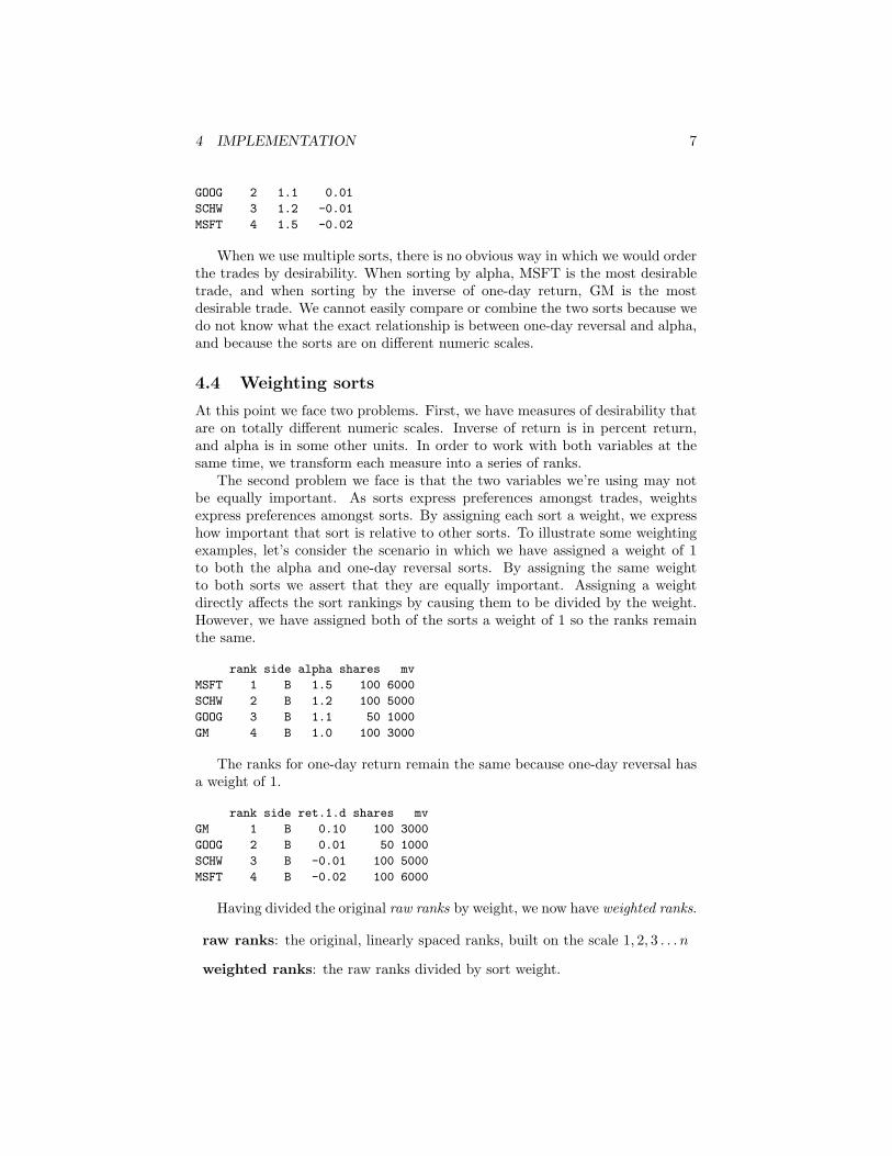
When we use multiple sorts, there is no obvious way in which we would orderthe trades by desirability. When sorting by alpha, MSFT is the most desirabletrade, and when sorting by the inverse of one-day return, GM is the mostdesirable trade. We cannot easily compare or combine the two sorts because wedo not know what the exact relationship is between one-day reversal and alpha,and because the sorts are on different numeric scales.

4.4 Weighting sorts

At this point we face two problems. First, we have measures of desirability thatare on totally different numeric scales. Inverse of return is in percent return,and alpha is in some other units. In order to work with both variables at thesame time, we transform each measure into a series of ranks.

The second problem we face is that the two variables we’re using may notbe equally important. As sorts express preferences amongst trades, weightsexpress preferences amongst sorts. By assigning each sort a weight, we expresshow important that sort is relative to other sorts. To illustrate some weightingexamples, let’s consider the scenario in which we have assigned a weight of 1to both the alpha and one-day reversal sorts. By assigning the same weightto both sorts we assert that they are equally important. Assigning a weightdirectly affects the sort rankings by causing them to be divided by the weight.However, we have assigned both of the sorts a weight of 1 so the ranks remainthe same.

rank side alpha shares mv

MSFT 1 B 1.5 100 6000

SCHW 2 B 1.2 100 5000

GOOG 3 B 1.1 50 1000

GM 4 B 1.0 100 3000

The ranks for one-day return remain the same because one-day reversal hasa weight of 1.

rank side ret.1.d shares mv

GM 1 B 0.10 100 3000

GOOG 2 B 0.01 50 1000

SCHW 3 B -0.01 100 5000

MSFT 4 B -0.02 100 6000

Having divided the original raw ranks by weight, we now have weighted ranks.

raw ranks: the original, linearly spaced ranks, built on the scale 1, 2, 3 . . . n

weighted ranks: the raw ranks divided by sort weight.

4 IMPLEMENTATION 8

We now have two ranks associated with each candidate, one from the alphasort and another from the one-day reversal sort. To illustrate that we haveduplicate ranks for each sort, we combine the equally-weighted alpha and one-day reversal sorts to form a single data frame.

rank sort side shares mv

MSFT.alpha 1 alpha B 100 6000

GM.ret.1.d 1 ret.1.d B 100 3000

SCHW.alpha 2 alpha B 100 5000

GOOG.ret.1.d 2 ret.1.d B 50 1000

GOOG.alpha 3 alpha B 50 1000

SCHW.ret.1.d 3 ret.1.d B 100 5000

GM.alpha 4 alpha B 100 3000

MSFT.ret.1.d 4 ret.1.d B 100 6000

The row names contain the equity ticker symbols and the name of the sortthat generated the rank. For each rank there are two candidates, one of whichhas been associated with a rank from alpha and the other which has been asso-ciated with a rank from one-day reversal. In cases such as this where we haveequally weighted sorts there will be a candidate trade from each sort at everyrank.

If we use n sorts, we will have n ranks associated with each candidate. Weonly want one rank associated with each candidate. So that each candidate onlyhas one rank associated with it, we assign each rank the best rank generated forit by any sort. We have done this in the data frame below.

rank shares mv

GM 1 100 3000

MSFT 1 100 6000

GOOG 2 50 1000

SCHW 2 100 5000

Both GM and MSFT have been assigned a rank of one. This occurs becauseMSFT has been ranked 1 by the alpha sort and GM has been ranked 1 by theone-day reversal sort. SCHW has been ranked 2 by the alpha sort and GOOGhas been ranked 3 by the alpha sort.

When we equally weight the sorts we are equally likely to use ranks fromeither sort. This behaviour is logical because assigning sorts equal weights sug-gests that they are equally important. However, the sorts may not always beequally important. In the next example we use a weighting scheme that causesus to use one sort to the exclusion of the other.

Let’s say that we do not want to consider one-day reversal. To ignore allof the one-day reversal values, we make alpha 10 times more important thanone-day reversal. Therefore, we will consider 10 ranks from alpha for every onerank from one-day reversal. As there are only 4 candidate trades, we will choosethe rankings in alpha over all ranks in the one-day reversal sort.

rank side shares mv

MSFT.alpha 0.1 B 100 6000

4 IMPLEMENTATION 9

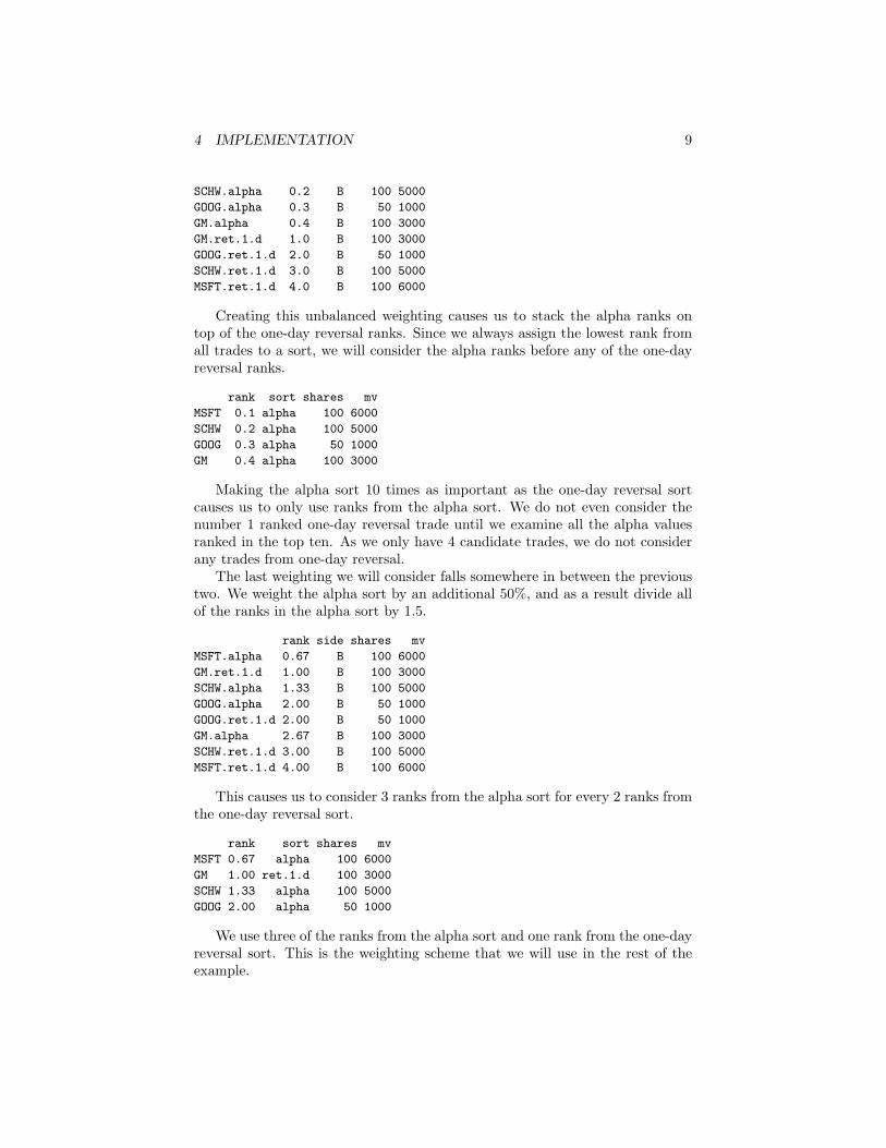
SCHW.alpha 0.2 B 100 5000

GOOG.alpha 0.3 B 50 1000

GM.alpha 0.4 B 100 3000

GM.ret.1.d 1.0 B 100 3000

GOOG.ret.1.d 2.0 B 50 1000

SCHW.ret.1.d 3.0 B 100 5000

MSFT.ret.1.d 4.0 B 100 6000

Creating this unbalanced weighting causes us to stack the alpha ranks ontop of the one-day reversal ranks. Since we always assign the lowest rank fromall trades to a sort, we will consider the alpha ranks before any of the one-dayreversal ranks.

rank sort shares mv

MSFT 0.1 alpha 100 6000

SCHW 0.2 alpha 100 5000

GOOG 0.3 alpha 50 1000

GM 0.4 alpha 100 3000

Making the alpha sort 10 times as important as the one-day reversal sortcauses us to only use ranks from the alpha sort. We do not even consider thenumber 1 ranked one-day reversal trade until we examine all the alpha valuesranked in the top ten. As we only have 4 candidate trades, we do not considerany trades from one-day reversal.

The last weighting we will consider falls somewhere in between the previoustwo. We weight the alpha sort by an additional 50%, and as a result divide allof the ranks in the alpha sort by 1.5.

rank side shares mv

MSFT.alpha 0.67 B 100 6000

GM.ret.1.d 1.00 B 100 3000

SCHW.alpha 1.33 B 100 5000

GOOG.alpha 2.00 B 50 1000

GOOG.ret.1.d 2.00 B 50 1000

GM.alpha 2.67 B 100 3000

SCHW.ret.1.d 3.00 B 100 5000

MSFT.ret.1.d 4.00 B 100 6000

This causes us to consider 3 ranks from the alpha sort for every 2 ranks fromthe one-day reversal sort.

rank sort shares mv

MSFT 0.67 alpha 100 6000

GM 1.00 ret.1.d 100 3000

SCHW 1.33 alpha 100 5000

GOOG 2.00 alpha 50 1000

We use three of the ranks from the alpha sort and one rank from the one-dayreversal sort. This is the weighting scheme that we will use in the rest of theexample.

4 IMPLEMENTATION 10

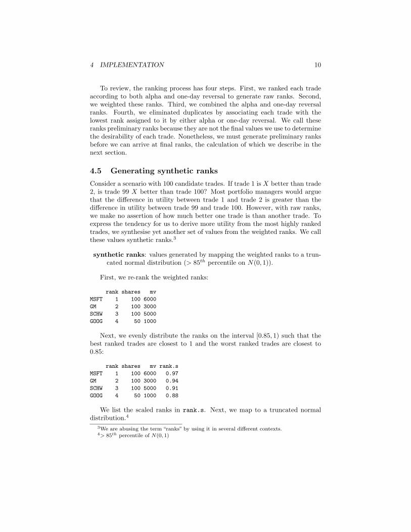
To review, the ranking process has four steps. First, we ranked each tradeaccording to both alpha and one-day reversal to generate raw ranks. Second,we weighted these ranks. Third, we combined the alpha and one-day reversalranks. Fourth, we eliminated duplicates by associating each trade with thelowest rank assigned to it by either alpha or one-day reversal. We call theseranks preliminary ranks because they are not the final values we use to determinethe desirability of each trade. Nonetheless, we must generate preliminary ranksbefore we can arrive at final ranks, the calculation of which we describe in thenext section.

4.5 Generating synthetic ranks

Consider a scenario with 100 candidate trades. If trade 1 is X better than trade2, is trade 99 X better than trade 100? Most portfolio managers would arguethat the difference in utility between trade 1 and trade 2 is greater than thedifference in utility between trade 99 and trade 100. However, with raw ranks,we make no assertion of how much better one trade is than another trade. Toexpress the tendency for us to derive more utility from the most highly rankedtrades, we synthesise yet another set of values from the weighted ranks. We callthese values synthetic ranks.3

synthetic ranks: values generated by mapping the weighted ranks to a trun-cated normal distribution (> 85th percentile on N(0, 1)).

First, we re-rank the weighted ranks:

rank shares mv

MSFT 1 100 6000

GM 2 100 3000

SCHW 3 100 5000

GOOG 4 50 1000

Next, we evenly distribute the ranks on the interval [0.85, 1) such that thebest ranked trades are closest to 1 and the worst ranked trades are closest to0.85:

rank shares mv rank.s

MSFT 1 100 6000 0.97

GM 2 100 3000 0.94

SCHW 3 100 5000 0.91

GOOG 4 50 1000 0.88

We list the scaled ranks in rank.s. Next, we map to a truncated normaldistribution.4

3We are abusing the term “ranks” by using it in several different contexts.4> 85th percentile of N(0, 1)

4 IMPLEMENTATION 11

rank shares mv rank.s rank.t

MSFT 1 100 6000 0.97 1.9

GM 2 100 3000 0.94 1.6

SCHW 3 100 5000 0.91 1.3

GOOG 4 50 1000 0.88 1.2

The rank.t column lists the ranks mapped to a truncated normal distribu-tion. MSFT has the best rank and GOOG has the worst rank. We might expectto see a rank.t of approximately 3.5 for the best ranked trade, but because weonly have 4 candidates and the scaled values are evenly spaced on the interval[0.85, 1), the normalised value of the best ranked trade is not as great as it wouldbe if we had 100 trades.

Recall that synthetic ranks express the tendency for there to be greater dif-ferences in desirability between adjacent, highly ranked trades (1, 2, 3 . . . ) thanbetween adjacent, poorly ranked trades:

rank ∆ N(0, 1) ∆ > 85th of N(0, 1) ∆1 1 3.50 1.17 3.50 0.532 1 2.32 0.27 2.96 0.213 1 2.05 0.17 2.74 0.134 1 1.88 0.13 2.61 0.105 1 1.75 0.11 2.51 0.08. . . . . .. . . . . .

48 1 0.05 0.03 1.46 0.0149 1 0.02 0.02 1.45 0.0150 1 0.00 0.02 1.44 0.0151 1 -0.02 0.02 1.43 0.0152 1 -0.05 0.03 1.42 0.01

. . . . . .

. . . . . .96 1 -1.64 0.11 1.06 0.0097 1 -1.75 0.13 1.06 0.0098 1 -1.88 0.17 1.06 0.0099 1 -2.05 0.27 1.06 0.00

100 - -2.32 - 1.06 -

Table 1: Creating synthetic ranks using a linear distribution, a normal distribu-tion, and a truncated normal distribution. Delta columns express the differencein desirability between adjacent trades.

Table 1 expresses the differences amongst distributions we might use to rank100 trades. The rank column contains the raw ranks for the 5 best trades, the5 middle-ranked trades, and the 5 worst trades. In this example the ranks on[1, 100] are spaced on intervals of one. The rank difference between every trade

4 IMPLEMENTATION 12

is the same. The difference between trade 1 and trade 2 is the same as thedifference between trade 99 and trade 100.

The normal distribution column (N(0, 1)) expresses what happens when wenormalise the raw ranks. The normal distribution correctly expresses our beliefthat there is a large difference in desirability between the best ranked trades.However, use of the normal distribution would incorrectly suggest that there aresimilarly large desirability differences between the worst trades. We get theseresults when using the normal distribution because the best and worst rankedtrades lie in the tails of the distribution. We do not want large differencesin desirability amongst the worst ranked trades. The desirability differencesdecrease until we reach trade 50, then increase again as we move towards theother tail of the distribution. We want desirability to remain the same on themargin past the 50th trade.

To address the problems associated with normalising to N(0, 1), we normaliseto a normal distribution truncated below the 85th percentile. In the rightmostdelta (∆) column, the synthetic rank differences between the best ranked tradesare over 50 times greater than the synthetic rank differences between the middleranked trades. Every trade ranked worse than 50 has a similar synthetic rankdifference. Although the subset [0.85, 1) is slightly arbitrary, (we could haveset the lower extreme to be 0.84, 0.86, or another similar value) it serves ourpurpose of expressing large differences in desirability where we find the bestbuys, on one tail, and small differences in desirability amongst the worst buys,on the other.

Recall the steps we have taken towards generating our final synthetic rank.First, we converted the sort values to raw ranks. Second, we converted theraw ranks to weighted ranks. Third, we scaled the weighted ranks to [0.85, 1)to generate scaled weights. Lastly, we mapped the scaled weights to a trun-cated normal distribution for our final synthetic rank. By only using the 85th

percentile and above, we express our belief that the differences in desirability be-tween the best ranked trades is much greater than the differences in desirabilitybetween the worst ranked trades.

If the costs associated with trading any stock, all things being equal, werethe same, we would not care about the difference in utility between trades. Wewould move down the trade list from best to worst until we reached our allottedturnover. However, our trading influences prices and may reduce the desirabilityof a trade.

4.6 Chunks, synthetic rank, and trade-cost adjustment

We want to know at what point the cost of trading an equity exceeds the utilityof trading that equity. In the portfolio package, we use synthetic rank torepresent utility. Determining the cost of purchasing an additional share isimpossible if our smallest trading unit is an entire order so we break each orderinto chunks.

chunk: A portion of a candidate trade.

4 IMPLEMENTATION 13

We break candidate trades into chunks by market value. Each chunk has amarket value of approximately $2000:

side shares mv alpha ret.1.d rank.t chunk.shares chunk.mv

MSFT.1 B 100 6000 1.5 -0.02 1.9 33 1980

MSFT.2 B 100 6000 1.5 -0.02 1.9 33 1980

MSFT.3 B 100 6000 1.5 -0.02 1.9 33 1980

MSFT.4 B 100 6000 1.5 -0.02 1.9 1 60

GM.1 B 100 3000 1.0 0.10 1.6 67 2010

GM.2 B 100 3000 1.0 0.10 1.6 33 990

SCHW.1 B 100 5000 1.2 -0.01 1.3 40 2000

SCHW.2 B 100 5000 1.2 -0.01 1.3 40 2000

SCHW.3 B 100 5000 1.2 -0.01 1.3 20 1000

GOOG.1 B 50 1000 1.1 0.01 1.2 50 1000

The candidate trades are broken into 10 chunks. The number followingthe ticker in the row name expresses the chunk number for that particularequity. The chunks.mv column expresses the market value of each chunk. Thechunk.shares column expresses how many shares are in each chunk.

4.6.1 Trade-cost adjustment of individual chunks

As we trade a greater percentage of the average daily volume, the price of thetrades will increase. To reflect this phenomenon, we penalise the synthetic ranksof the chunk as we trade greater percentages of the daily volume. We call thispenalty trade-cost adjustment.

trade-cost adjustment: Lowering a chunk’s rank because of trading volume.

To fix this idea, let’s first examine the daily volumes of our candidate trades.5

rank.t volume shares

MSFT 1.9 2600 100

GM 1.6 100 100

SCHW 1.3 2500 100

GOOG 1.2 2200 50

The trades we want to make for MSFT, SCHW, and GOOG involve lessthan 3% of the daily trading volume. However, we want to trade 100% of thedaily trading volume of GM. We would probably not be able to purchase all ofthese shares in one day, and even if we could, we would affect prices significantly.Moving into the position over several days would be better.

We use a trade-cost adjustment function to express how increasing tradecosts reduce the desirability of candidate trades. To better approximate utility,we penalise synthetic ranks at the chunk level. Doing this allows us to better

5The volume column represents some measure of past trading volume such as the averagetrading volume over the last 30 days. A daily measure of volume is not required; we woulduse whatever measure is natural for the frequency with which we trade.

4 IMPLEMENTATION 14

determine at which point the cost of trading an additional chunk is greaterthan the utility derived by trading an additional chunk. We perform trade-cost adjustment on the chunks by keeping track of what percentage of the dailyvolume we have traded with each additional chunk. In the trade-cost adjustmentfunction used in this example, the first chunk to cross the threshold of 15% ofthe daily trading volume is penalised by a fixed amount. All subsequent chunksare penalised by that amount, and any further chunks that pass 30% or 45%percent of the daily trading volume receive further penalties. The function usedin this example also prevents any adjustment on the first chunk of a candidatetrade. Below, we can see that the second chunk of the trade for GM has beentrade-cost adjusted:

side mv alpha ret.1.d rank.t chunk.shares chunk.mv tca.rank

MSFT.1 B 6000 1.5 -0.02 1.9 33 1980 1.9

MSFT.2 B 6000 1.5 -0.02 1.9 33 1980 1.9

MSFT.3 B 6000 1.5 -0.02 1.9 33 1980 1.9

MSFT.4 B 6000 1.5 -0.02 1.9 1 60 1.9

GM.1 B 3000 1.0 0.10 1.6 67 2010 1.6

GM.2 B 3000 1.0 0.10 1.6 33 990 -4.4

SCHW.1 B 5000 1.2 -0.01 1.3 40 2000 1.3

SCHW.2 B 5000 1.2 -0.01 1.3 40 2000 1.3

SCHW.3 B 5000 1.2 -0.01 1.3 20 1000 1.3

GOOG.1 B 1000 1.1 0.01 1.2 50 1000 1.2

The tca.rank column expresses the synthetic rank adjusted for trade costs.Since GM is the only candidate for which we want to purchase more than 15% ofthe daily trading volume, it is the only candidate for which we trade-cost adjustthe chunks. Every chunk of GM beyond the first has been trade-cost adjusted.This will cause us to consider the chunks of other candidate trades before wetrade additional chunks of GM:


MSFT.1 B 6000 1.5 -0.02 1.9 33 1980 1.9

MSFT.2 B 6000 1.5 -0.02 1.9 33 1980 1.9

MSFT.3 B 6000 1.5 -0.02 1.9 33 1980 1.9

MSFT.4 B 6000 1.5 -0.02 1.9 1 60 1.9

GM.1 B 3000 1.0 0.10 1.6 67 2010 1.6

SCHW.1 B 5000 1.2 -0.01 1.3 40 2000 1.3

SCHW.2 B 5000 1.2 -0.01 1.3 40 2000 1.3

SCHW.3 B 5000 1.2 -0.01 1.3 20 1000 1.3

GOOG.1 B 1000 1.1 0.01 1.2 50 1000 1.2

GM.2 B 3000 1.0 0.10 1.6 33 990 -4.4

As MSFT is the best ranked candidate and does not receive a trade-costpenalty, we would trade all the shares of MSFT before considering the othercandidates.6 Having completed all the chunks of MSFT, we would consider the

6Assuming that derived turnover is greater than the market value of all the candidatetrades.

4 IMPLEMENTATION 15

first chunk of GM, the only chunk which has not been trade-cost adjusted. Sub-sequently, we would trade all the chunks of SCHW and GOOG, the candidatetrades ranked 3 and 4. Lastly, we trade the penalised chunk of GM.

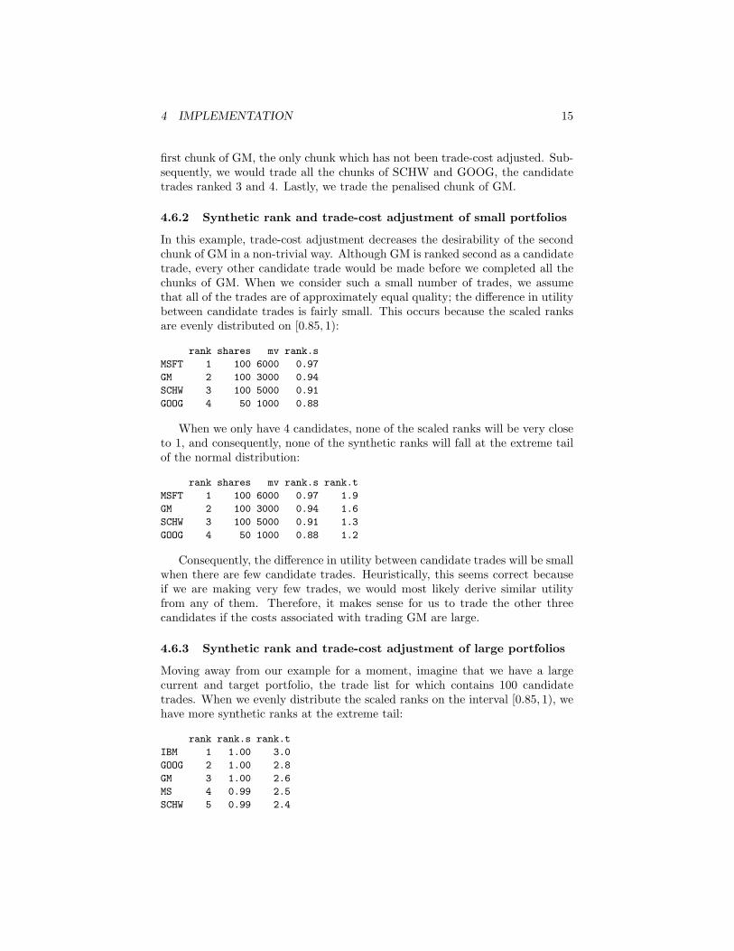
4.6.2 Synthetic rank and trade-cost adjustment of small portfolios

In this example, trade-cost adjustment decreases the desirability of the secondchunk of GM in a non-trivial way. Although GM is ranked second as a candidatetrade, every other candidate trade would be made before we completed all thechunks of GM. When we consider such a small number of trades, we assumethat all of the trades are of approximately equal quality; the difference in utilitybetween candidate trades is fairly small. This occurs because the scaled ranksare evenly distributed on [0.85, 1):

rank shares mv rank.s

MSFT 1 100 6000 0.97

GM 2 100 3000 0.94

SCHW 3 100 5000 0.91

GOOG 4 50 1000 0.88

When we only have 4 candidates, none of the scaled ranks will be very closeto 1, and consequently, none of the synthetic ranks will fall at the extreme tailof the normal distribution:

rank shares mv rank.s rank.t

MSFT 1 100 6000 0.97 1.9

GM 2 100 3000 0.94 1.6

SCHW 3 100 5000 0.91 1.3

GOOG 4 50 1000 0.88 1.2

Consequently, the difference in utility between candidate trades will be smallwhen there are few candidate trades. Heuristically, this seems correct becauseif we are making very few trades, we would most likely derive similar utilityfrom any of them. Therefore, it makes sense for us to trade the other threecandidates if the costs associated with trading GM are large.

4.6.3 Synthetic rank and trade-cost adjustment of large portfolios

Moving away from our example for a moment, imagine that we have a largecurrent and target portfolio, the trade list for which contains 100 candidatetrades. When we evenly distribute the scaled ranks on the interval [0.85, 1), wehave more synthetic ranks at the extreme tail:

rank rank.s rank.t

IBM 1 1.00 3.0

GOOG 2 1.00 2.8

GM 3 1.00 2.6

MS 4 0.99 2.5

SCHW 5 0.99 2.4

4 IMPLEMENTATION 16

MSFT 48 0.92 1.4

T 49 0.92 1.4

CVX 50 0.92 1.4

AET 96 0.86 1.1

AMD 97 0.86 1.1

DELL 98 0.85 1.1

EBAY 99 0.85 1.0

HPQ 100 0.85 1.0

The row names express the equity ticker symbols. rank is the raw rank.rank.s is the scaled rank, and rank.t is the synthetic rank. The best rankedtrade, IBM, has a scaled rank value very close to one and a synthetic rankclose to three. This indicates that the best rank falls at the tail of the normaldistribution. The worst ranked candidates not only have low synthetic ranks,but they also have very small differences in synthetic rank. If we trade-costadjust one of the poorly ranked candidates we will most likely not trade it untilwe have traded all other candidates not penalised by trade cost adjustment. Onthe other hand, we would still trade IBM, GOOG, or GM, even if some of thechunks had been trade-cost adjusted.

Let’s quickly review how we generate the final, synthetic ranks. The pre-liminary values from which we draw the raw ranks are the sorts we define. Inthis example, we defined sorts for alpha and one-day reversal. In creating rawranks, we ignore the underlying values used by the sorts. At this point, we stillhave a different set of raw ranks for each sort. To express preferences amongstthe sorts, we apply weights to the sorts. This step yields weighted ranks. Fromthe sets of weighted ranks, we associate with each candidate the best weightedrank from any sort. Next, we scale the buys to the interval [0.85, 1). This stepyields scaled ranks. From scaled ranks, we generate synthetic ranks by mappingthe scaled ranks to a truncated normal distribution. Next, we break the candi-dates into chunks and perform trade-cost adjustment as necessary. This yieldstrade-cost adjusted ranks which are the final measure of chunks’ desirability.

4.7 Sorting theory

Chooing the best candidate when we have multiple measures of desirability isdifficult. Consider the situation where we must choose ten stocks to trade.

In our example, assuming that we use some type of formula to generatealpha, we might be able to incorporate our other sorts into the formula foralpha. Instead of having alpha and one-day reversal as distinct sorts, we wouldonly have one sort, alpha, which would also take one-day reversal into account.For this to work, however, we would have to write a function that accountedfor the the ordering of every trade by every sort. Furthermore, this functionwould have to take into account our preference for certain sorts over other sorts.To elaborate on how difficult it is to create such a function, let us consider thesituation where we must choose our ten favourite trades, in no particular order,using the data in the table below.

4 IMPLEMENTATION 17

symbol raw rank alpha symbol raw rank one-day returnIBM 1 1.57 HPQ 1 -0.063MS 2 1.26 SUNW 2 -0.056

EBAY 3 1.24 AET 3 -0.041CBBO 4 1.21 YHOO 4 -0.036SCHW 5 1.15 T 5 -0.014PAYX 6 1.12 CVX 6 -0.011HAL 7 1.12 GOOG 7 -0.011AMD 8 1.10 PAYX 8 -0.002

MSFT 9 0.99 CBBO 9 0.003CVX 10 0.96 HAL 10 0.009AET 11 0.92 QCOM 11 0.011HPQ 12 0.81 EBAY 12 0.014

QCOM 13 0.77 SCHW 13 0.029GOOG 14 0.65 AAPL 14 0.036YHOO 15 0.64 MS 15 0.041

Table 2: The alpha and one-day returns of candidates suggest different rankorderings. All of the candidates are buys.

Table 2 has a row for each of 15 candidates, their alpha and one-day reversalvalues, and the raw ranks we would generate from these values. All of thecandidates are buys so greater alpha values are better and lesser one-day reversalvalues are better.

One portfolio manager might decide that she wants to make trades basedonly on alpha. She chooses the top ten trades according to alpha. A secondportfolio manager may want to make trades based only on one-day return. Shechooses the top ten trades according to one-day return. The third portfoliomanager considers both alpha and one-day return and choose her favorite tradesby examining both.

Portfolio manager three believes in buying equities which have had pricedecreases of greater than 4% during the previous trading day. Consequently,she would buy HPQ, SUNW, and AET. She would fill her remaining ordersusing the top 7 trades according to alpha.

How would the third portfolio manager write a function that expresses hertrading preferences? What if some days she acted like the first portfolio managerand on other days like the second portfolio manager? How would she accountfor a change in preference for one of the sorts?

Our solution allows any of these portfolio managers to express her tradingpreferences without having to write a function that relates the different mea-sures of desirability. Instead, she would use the weighting function that theportfolio package provides. She would examine the trade list created usingdifferent weighting schemes and adjust the weights until the utility derived fromthe last candidate traded was greater than the cost of the first trade not made.

For example, the portfolio manager may decide that YHOO is a better re-

4 IMPLEMENTATION 18

versal trade than the last alpha trade and revise the weighting scheme so thatshe makes one less alpha trade and one more reversal trade.

symbol raw rank alpha symbol raw rank ret.1.dIBM 1 1.57 HPQ 1 -0.063MS 2 1.26 SUNW 2 -0.056

EBAY 3 1.24 AET 3 -0.041CBBO 4 1.21 YHOO 4 -0.036SCHW 5 1.15 T 5 -0.014PAYX 6 1.12 CVX 6 -0.011HAL 7 1.12 GOOG 7 -0.011AMD 8 1.10 PAYX 8 -0.002

MSFT 9 0.99 CBBO 9 0.003CVX 10 0.96 HAL 10 0.009AET 11 0.92 QCOM 11 0.011HPQ 12 0.81 EBAY 12 0.014

QCOM 13 0.77 SCHW 13 0.029GOOG 14 0.65 AAPL 14 0.036YHOO 15 0.64 MS 15 0.041

Table 3: Portfolio manager 3 revises her trading preferences.

What ultimately matters is the last candidate we decide to trade and the firstcandidate we decide not to trade. By using rank orders instead of underlyingvalues, we do not have to combine the different sorts. Instead, we can expressour preferences for different, possibly unrelated criteria through the use of aweighting scheme we provide in portfolio.

4.8 Pairing trades

Let us return to discussing trade list construction. In practise, most equityportfolios must be maintained at a specific market value. One logical way toachieve this result would be to pair desirable buys and sells of equal marketvalue, which is what we do in the portfolio package. We call these pairings ofbuys and sells a swap:

swap: A pairing of a buy and sell or short and cover of similar market marketvalue and desirability.

We have already created the framework to create swaps; we break the can-didates into chunks of similar market value and then rank these chunks individ-ually. If our candidate trades included buys and sells, we would simply matchthe most desirable buys with the most desirable sells. However, our candidatetrades are all buys, and we want to increase the market value of our portfolioby $1,000.

4 IMPLEMENTATION 19

4.8.1 Dummy chunks

If we want to increase the market value of the portfolio, we must buy more thanwe sell. Therefore, we do not want to pair a buy with a sell. We just want buys.The situation where we just want buys or sells is a special case. The portfoliopackage is structured so that we must also trade in pairs. To work within thepackage framework we introduce the concept of dummy chunks:

dummy chunk: A fake buy or sell chunk that we pair with a real buy orsell chunk in situations where we want to increase or decrease the marketvalue of the portfolio.

As our example only contains buys, we have paired every buy with a dummysell.7

tca.rank.enter tca.rank.exit rank.gain

MSFT.1,NA.0 1.9 10000 -9998

MSFT.2,NA.0 1.9 10000 -9998

MSFT.3,NA.0 1.9 10000 -9998

MSFT.4,NA.0 1.9 10000 -9998

GM.1,NA.0 1.6 10000 -9998

SCHW.1,NA.0 1.3 10000 -9999

In the table above, the row names express the chunk ticker symbols thatform the swap. To the left of the comma is an enter chunk, and to the right ofthe comma is an exit chunk.8 The exit chunks all have a symbol NA.0 becausethey are dummy sells. The tca.rank.enter column expresses the trade-costadjusted rank of the enter chunk, the buy, and the tca.rank.exit columnexpresses the trade-cost adjusted rank of the exit chunk, the dummy sell. Therank.gain column expresses the difference in trade-cost adjusted rank betweenthe enter and the exit, the buy and dummy sell.

We have spent considerable time discussing the generation of all types ofranks for buys, but we have not yet discussed ranking sells. For sells, betterranks are more negative. Therefore, a great sell might have a synthetic rank of-3.5.

Recall that our goal is to make the trades which yield the most utility.In spending our $1,000, we want to trade the best chunks. So that we makethe best buys when increasing the market value of the portfolio, we assign thedummy sells an arbitrarily high rank. In the table above, the dummy sells havea trade-cost adjusted rank of -10,000. We match the best the buys and sells bycalculating rank gain. As no real sells will yield the same rank gain that thepairing of buy and a dummy sell yields, we create pairs with all the dummy sellsbefore even considering other sells. As there are no sells in this example, all theswaps consist of a buy and a dummy sell.

7We only show the head of the swaps table.8Enter chunks are either a buy or short. A buy allows us to take a long position and a

short allows us to take a short position. Exit chunks are either sells or covers. A sell allowsus to exit a long position and a cover allows us to exit a short position.

4 IMPLEMENTATION 20

Let’s quickly review why we create swaps. We want to maximise utilityby making the candidate trades or portions of candidate trades that yield thegreatest utility. Generally, we want to maintain the portfolio equity at a constantlevel. A logical way to do this involves pairing buys and sells of similar marketvalue. To maximise utility, we should pair the most best ranked buys andsells. In special cases, we want to increase or decrease the market value of ourportfolio. In order to do this, we must make more of one type of trade. However,this would require that we have swaps that contain only a buy or sell. Since wecannot have a swap of only one trade, we introduce dummy trades. As dummytrades have an arbitrarily high synthetic rank they pair with the best buys andsells to ensure that we choose the most useful candidates in changing the marketvalue of the portfolio.

4.9 Accounting for turnover

Note: this and subsequent sections need to account for change in turnover appli-cation. Now all swaps are done such that the total market value of trades goesup to but doesn’t exceed the turnover amount. In the meantime I have adjustedthe example’s turnover to $2,000 so that at least one chunk is done, althoughnow Sweave chunks will be inconsistent with the text.

As we stated earlier, holding period would be endogenous if we could alwaysset it to maximise risk-adjusted return. However, most real world portfolios havea set holding period and consequently, a set turnover. There is no real conceptof turnover or holding period in this example. We have $1,000 to invest in ourportfolio over the course of a single day. Although this additional investmentdoes not represent turnover, we can view our $1,000 as representing a dailyturnover of $1,000. We want to make the best ranked trades until the cumulativemarket value of these trades exceeds the money we have to invest. Analogously,we would say that we want to make the best ranked trades until we exceedturnover.

As our turnover in this example is $2000, all of our trades will not have amarket value greater than $2000:

tca.rank.enter tca.rank.exit rank.gain

MSFT.1,NA.0 1.9 10000 -9998

MSFT is the the best ranked trade. Consequently, we choose swaps of MSFTbefore choosing other swaps. We make 1 because each swap has a value ofapproximately $2000, and our turnover is $2000.

4.10 Actual orders

We do not want to submit two orders for 8 shares of MSFT. Before submittingthe trade list, we must roll-up the swaps into larger orders. We first remove thedummy chunks:

5 CREATING A LONG-ONLY TRADELIST IN R 21


MSFT.1 B 6000 1.5 -0.02 1.9 33 1980 1.9

Then we combine the chunks to form a single order per candidate:

side shares mv alpha ret.1.d rank.t

MSFT B 33 1980 1.5 -0.02 1.9

We now have an order for 33 shares of MSFT, which is the sum of thechunks of MSFT. Having discussed in words the process of trade list creation,we describe, step-by-step, the process of building a tradelist object in R.

5 Creating a long-only tradelist in R

To create a tradelist, we need four main pieces. The first two pieces necessaryto create a tradelist are portfolio objects. One of these portfolios is ourcurrent portfolio.

Our current portfolio is a superset of the previous holdings. The majordifference between the two portfolios is that the current portfolio in this exampleincludes positions that we sell. This portfolio, named p.current, consists of6 positions and has a market value of $47,750.

> p.current.shares

shares price

IBM 100 10

GM 100 30

EBAY 75 120

DELL 50 110

QCOM 75 190

AMD 150 100

The target portfolio is a superset of the previous target portfolio. It contains6 positions and has a market value of $47,500.

> p.target.shares

shares price

GOOG 50 20

EBAY 75 120

IBM 100 10

GM 200 30

SCHW 100 50

MSFT 100 60

AMD 100 100

QCOM 50 190

We calculate the portfolio difference to determine the candidate trades.9

9The data frame is a subset of the candidates data frame. We often take subsets of dataframes so that they fit better on the page. If we do so we indicate this by prepending thename of the data frame with sub.

5 CREATING A LONG-ONLY TRADELIST IN R 22

> sub.candidates

orig target side shares mv

AMD 150 100 S 50 -5000

DELL 50 0 S 50 -5500

GM 100 200 B 100 3000

GOOG 0 50 B 50 1000

MSFT 0 100 B 100 6000

QCOM 75 50 S 25 -4750

SCHW 0 100 B 100 5000

The candidate buys are the same as before and we have 3 candidate sells.The market value is signed and expresses the net effect a candidate has on thedollar value of a portfolio.

5.1 Assigning weights

We assign weights to the sorts by creating a list.

> sorts <- list(alpha = 1, ret.1.d = 1.1)

We assign a weight of 1 to alpha and a weight of 1.1 to one-day return.

5.2 Passing additional information to tradelist

The fourth item is a data frame. The portfolio package requires that this dataframe contain columns for id, volume, price.usd, and the sorts:

> sub.data

id volume price.usd alpha ret.1.d

IBM IBM 2100 10 -0.76 -0.003

GOOG GOOG 2200 20 1.10 0.010

GM GM 100 30 1.00 0.100

SCHW SCHW 2500 50 1.20 -0.010

MSFT MSFT 2600 60 1.50 -0.020

AMD AMD 3000 100 -0.94 0.010

DELL DELL 3100 110 -0.15 0.070

EBAY EBAY 3200 120 -0.32 0.001

QCOM QCOM 3900 190 -0.36 -0.005

volume expresses some measure of average trading volume. price.usd isthe most recent price of the security in US dollars. We must also include thesorts we define in sorts, alpha and ret.1.d.

5.3 Calling new

We use p.current, p.target, the sorts, and data as arguments to new.

6 THE TRADELIST ALGORITHM 23

> tl <- new("tradelist", orig = p.current, target = p.target,

+ chunk.usd = 2000, sorts = sorts, turnover = 30250, data = data)

In this call, the new method for tradelist accepts 8 parameters:10 The firstargument, "tradelist", specifies the name of the object that we want to create.The argument to the orig parameter, p.current, is the current portfolio. Theargument to the target parameter, p.current, is the target portfolio. Thesorts parameter accepts the sorts list we created earlier. We create chunkswith a granularity of of $2,000. The data parameter accepts the data frame wecreated earlier with columns for id, volume, price.usd, and the sorts.

The turnover parameter accepts an integer argument which expresses themaximum market value all orders made in one session. In the previous examplewe only had $1,000 with which we could buy stocks. In this example, we canboth buy and sell equities. We might sell an equity and use the proceeds to buyanother equity. However, the turnover restriction applies to sells just as muchas buys. If we have a turnover of $1,000, we may make $1,000 worth of buys,$1,000 worth of sells, or something in between. For this example, we have set theturnover equal to the unsigned market value of all the candidate trades. Thismeans that we take the absolute value of all market values, which is $30,250.Having set turnover to this value, we complete every candidate trade.

We have demonstrated how to create a simple tradelist in R. In the nextsection we examine the tradelist that we have constructed. In doing so, welearn how the tradelist generation algorithm works.

6 The tradelist algorithm

The tradelist code provides an algorithm, divisible into seven smaller steps,that generates a set of trades that will move the current, original portfolio to-wards an ideal, target portfolio. The seven steps in the algorithm correspondto the following methods of the tradelist class: calcCandidates, calcRanks,calcChunks, calcSwaps, calcSwapsActual, calcChunksActual, and calcActual.

The user never needs to directly call any of these methods when using theportfolio package. A call to the new method of the tradelist class invokesthe initialize method of tradelist. The initialize method then callsthe seven methods serially. The first step of the tradelist algorithm involvesdetermining which types of orders we must make in order to trade towards thetarget portfolio.

6.1 The calcCandidates method

As stated in our simplifying assumption, we only consider trades that bring uscloser to the target portfolio. To determine candidate trades we calculate whichpositions have changed. If a position has changed, we determine what type of

10The new method of tradelist can accept more parameters, but they are optional.


trade the candidate is (buy or sell) by taking the portfolio difference to generatea list of candidate trades.

> tl@candidates

id orig target side shares mv

AMD AMD 150 100 S 50 -5000

DELL DELL 50 0 S 50 -5500

GM GM 100 200 B 100 3000

GOOG GOOG 0 50 B 50 1000

MSFT MSFT 0 100 B 100 6000

QCOM QCOM 75 50 S 25 -4750

SCHW SCHW 0 100 B 100 5000

Given the data stored in the candidates data frame and the data dataframe, the portfolio package can generate the trade list.

6.2 The calcRanks Method

Ranking the trades is possibly the most complicated task delegated to thetradelist class. When the rank-generating algorithm returns, the ranks dataframe tradelist will contain the synthetic rank, rank.t, for each trade.

6.2.1 Interpretation of sort values

When we define a sort, we express our preference for purchasing different stocks.Lesser values express a preference for selling or shorting a position and greatervalues express a preference for buying or covering a position. In the previousexample we only saw positive alpha values because all the candidates were buys.If the values were not positive, we might question why the trade was even acandidate. Recall our first simplifying assumption that all of the candidates aredesirable and the portfolio package only helps us to determine which are themost desirable.

In real life, we want to create a sort using meaningful values that expressour trading preferences. One such value is one-day return.

6.2.2 Creating raw ranks for a long-only portfolio

The first step in creating ranks is generating raw ranks. We break the tradesinto separate data frames by side and rank the trades within each side becauseone type of trade is no than another type of trade.

$B

id orig target side shares mv ret.1.d rank

GM GM 100 200 B 100 3000 0.10 1

GOOG GOOG 0 50 B 50 1000 0.01 2

SCHW SCHW 0 100 B 100 5000 -0.01 3

MSFT MSFT 0 100 B 100 6000 -0.02 4


$S


QCOM QCOM 75 50 S 25 -4750 -0.005 1

AMD AMD 150 100 S 50 -5000 0.010 2

DELL DELL 50 0 S 50 -5500 0.070 3

The $B data frame shows the buys ranked with other buys and the $S dataframe shows the sells ranked with other sells. The most desirable buys arethose associated with the greatest values in ret.1.d. The most desirable sellsare those associated with the least value in ret.1.d. Therefore, GM ranked 1amongst buys, is the most desirable buy, and QCOM, ranked 1 amongst sells,is the most desirable sell.11

6.2.3 Interleaving

We now have two tables of ranks and there are still multiple trades at each rank:a buy and sell ranked number one, number two and so on. Combining the twotables of ranks by type leaves us with duplicates:

orig target side shares mv ret.1.d rank

GM 100 200 B 100 3000 0.100 1

QCOM 75 50 S 25 -4750 -0.005 1

GOOG 0 50 B 50 1000 0.010 2

AMD 150 100 S 50 -5000 0.010 2

SCHW 0 100 B 100 5000 -0.010 3

DELL 50 0 S 50 -5500 0.070 3

MSFT 0 100 B 100 6000 -0.020 4

We argue that there is no natural way to choose between the best buy andbest sell. To deal with this ambiguity, we always break ties in rank between abuy and sell by assigning the buy the higher rank. In the following table, wecreate new raw ranks to eliminate the duplicates.

orig target side shares mv alpha rank

MSFT 0 100 B 100 6000 1.50 1

AMD 150 100 S 50 -5000 -0.94 2

SCHW 0 100 B 100 5000 1.20 3

QCOM 75 50 S 25 -4750 -0.36 4

GOOG 0 50 B 50 1000 1.10 5

DELL 50 0 S 50 -5500 -0.15 6

GM 100 200 B 100 3000 1.00 7

Notice that each candidate has a unique rank and that the rows alternatebetween buy and sell candidates. The best ranked candidate trade is a buy

11We have taken the inverse of all the one-day return values so that the portfolio packageinterprets them correctly. If we believe one-day reversal, the best buys have negative one-dayreturns and the best sells have positive one-day returns. Buy low, sell high. However, theportfolio package interprets greater values as indicative of the best buys and lesser values asindicate of the best sells.


because we broke the tie for first between the best ranked buy and sell byassigning the buy the higher rank. This pattern repeats throughout the dataframe because we have ties at every rank except the last. We call this processof alternating between the best ranked buys and sells interleaving.

interleaving: The process of breaking the trades up by side and rankingthem with other trades of the same type, thereby yielding multiple tradesat each rank. We always break ties in rank with the following ordering:Buys, Sells, Covers, Shorts (B, S, C, X).

6.2.4 Weighted ranks

Having interleaved the candidates, we divide the new raw ranks by the weightassigned to one-day return, 1.1.


GM GM 100 200 B 100 3000 0.100 0.83

QCOM QCOM 75 50 S 25 -4750 -0.005 1.65

GOOG GOOG 0 50 B 50 1000 0.010 2.48

AMD AMD 150 100 S 50 -5000 0.010 3.31

SCHW SCHW 0 100 B 100 5000 -0.010 4.13

DELL DELL 50 0 S 50 -5500 0.070 4.96

MSFT MSFT 0 100 B 100 6000 -0.020 5.79

We assigned alpha a weight of 1 so the ranks remain the same.

> [email protected][["alpha"]]

id orig target side shares mv alpha rank

MSFT MSFT 0 100 B 100 6000 1.50 1

AMD AMD 150 100 S 50 -5000 -0.94 2

SCHW SCHW 0 100 B 100 5000 1.20 3

QCOM QCOM 75 50 S 25 -4750 -0.36 4

GOOG GOOG 0 50 B 50 1000 1.10 5

DELL DELL 50 0 S 50 -5500 -0.15 6

GM GM 100 200 B 100 3000 1.00 7

We combine the alpha and one-day return ranks into a single data frame.

id orig target side shares mv rank

1 AMD 150 100 S 50 -5000 2.0

2 AMD 150 100 S 50 -5000 3.6

3 DELL 50 0 S 50 -5500 6.0

4 DELL 50 0 S 50 -5500 5.5

5 GM 100 200 B 100 3000 7.0

6 GM 100 200 B 100 3000 0.9

7 GOOG 0 50 B 50 1000 5.0

8 GOOG 0 50 B 50 1000 2.7

9 MSFT 0 100 B 100 6000 1.0

10 MSFT 0 100 B 100 6000 6.4


11 QCOM 75 50 S 25 -4750 4.0

12 QCOM 75 50 S 25 -4750 1.8

13 SCHW 0 100 B 100 5000 3.0

14 SCHW 0 100 B 100 5000 4.5

To remove duplicates, we assign each candidate the best weighted rank as-sociated with it by any sort.


GM 100 200 B 100 3000

MSFT 0 100 B 100 6000

QCOM 75 50 S 25 -4750

AMD 150 100 S 50 -5000

GOOG 0 50 B 50 1000

SCHW 0 100 B 100 5000

DELL 50 0 S 50 -5500

And we re-rank the candidates.

target side shares mv rank.t

GM 200 B 100 3000 1.9

MSFT 100 B 100 6000 1.6

QCOM 50 S 25 -4750 -1.8

AMD 100 S 50 -5000 -1.4

GOOG 50 B 50 1000 1.3

SCHW 100 B 100 5000 1.2

DELL 0 S 50 -5500 -1.2

6.2.5 Mapping to the truncated normal distribution

Having weighted the ranks we create synthetic ranks from a truncated normaldistribution. When we only have buys, we scale the weighted ranks to [0.85, 1).This gives us the positive tail of the normal distribution. We associate morenegative values with better sells so we want to map sells to the negative tail ofthe normal distribution. To do this, we scale sells to the interval (0, 0.15].

side alpha ret.1.d rank rank.ws

QCOM S -0.36 -0.005 1.8 0.037

AMD S -0.94 0.010 2.0 0.075

DELL S -0.15 0.070 5.5 0.112

SCHW B 1.20 -0.010 3.0 0.880

GOOG B 1.10 0.010 2.7 0.910

MSFT B 1.50 -0.020 1.0 0.940

GM B 1.00 0.100 0.9 0.970

We map the scaled ranks to the normal distribution.

> tl.ranks


id orig target side shares mv alpha ret.1.d rank.t

QCOM QCOM 75 50 S 25 -4750 -0.36 -0.005 -1.8

AMD AMD 150 100 S 50 -5000 -0.94 0.010 -1.4

DELL DELL 50 0 S 50 -5500 -0.15 0.070 -1.2

SCHW SCHW 0 100 B 100 5000 1.20 -0.010 1.2

GOOG GOOG 0 50 B 50 1000 1.10 0.010 1.3

MSFT MSFT 0 100 B 100 6000 1.50 -0.020 1.6

GM GM 100 200 B 100 3000 1.00 0.100 1.9

rank.t expresses the synthetic rank. All of the sells have a negative rank.tbecause they have been mapped to the negative tail of the normal distribution,while all of the buys have a positive rank.t because they have been mapped tothe other tail. As described in section 4.6.3, the synthetic ranks do not fall atthe extreme tail of the normal distribution.

6.3 The calcChunks Method

Having calculated synthetic ranks, the portfolio package creates the chunkstable. We defined the market value of each chunk by specifying the chunk.usdparameter in the call to new. The addition of sells does not have a dramaticeffect on the manner in which we generate the chunk table besides contributingnegative trade-cost adjusted ranks.

> sub.chunks

side rank.t chunk.shares chunk.mv tca.rank

AMD.1 S -1.4 20 -2000 -1.4

AMD.2 S -1.4 20 -2000 -1.4

AMD.3 S -1.4 10 -1000 -1.4

DELL.1 S -1.2 18 -1980 -1.2

DELL.2 S -1.2 18 -1980 -1.2

DELL.3 S -1.2 14 -1540 -1.2

GM.1 B 1.9 67 2010 1.9

GM.2 B 1.9 33 990 -4.1

GOOG.1 B 1.3 50 1000 1.3

MSFT.1 B 1.6 33 1980 1.6

MSFT.2 B 1.6 33 1980 1.6

MSFT.3 B 1.6 33 1980 1.6

MSFT.4 B 1.6 1 60 1.6

QCOM.1 S -1.8 11 -2090 -1.8

QCOM.2 S -1.8 11 -2090 -1.8

QCOM.3 S -1.8 3 -570 -1.8

SCHW.1 B 1.2 40 2000 1.2

SCHW.2 B 1.2 40 2000 1.2

SCHW.3 B 1.2 20 1000 1.2

Most chunks have an unsigned market value of approximately $2,000. Theonly chunks of market value significantly less than $2,000 are the final chunksof a candidate. These chunks are the remainders left after dividing the rest ofthe order into $2,000 chunks.


If we order the chunks by tca.rank, the second chunk of GM has beenseverely penalised for trade costs.

> head(sub.chunks[order(sub.chunks[["tca.rank"]]), ])


GM.2 B 1.9 33 990 -4.1

QCOM.1 S -1.8 11 -2090 -1.8

QCOM.2 S -1.8 11 -2090 -1.8

QCOM.3 S -1.8 3 -570 -1.8

AMD.1 S -1.4 20 -2000 -1.4

AMD.2 S -1.4 20 -2000 -1.4

GM has a more negative tca.rank than any of the buys or sells, indicatingthat this is the last chunk we would trade.

6.4 The calcSwaps Method

The calcSwaps works in as it did in the previous example, the main differencebeing that we pair real buy chunks with real sell chunks. We determine whichtrades to pair for a swap by calculating rank gain.

rank gain: The difference in tca.rank between a buy and a sell. As themost desirable buys have a very positive tca.rank and the most desirablesells have a very negative tca.rank, the best swaps have great rank.gainvalues.

Buys with high tca.rank have been matched with sells with low tca.rank.

> swaps.sub

side.enter tca.rank.enter side.exit tca.rank.exit rank.gain

GM.1,QCOM.1 B 1.9 S -1.8 3.7

MSFT.1,QCOM.2 B 1.6 S -1.8 3.3

MSFT.2,QCOM.3 B 1.6 S -1.8 3.3

MSFT.3,AMD.1 B 1.6 S -1.4 3.0

MSFT.4,AMD.2 B 1.6 S -1.4 3.0

GOOG.1,AMD.3 B 1.3 S -1.4 2.8

SCHW.1,DELL.1 B 1.2 S -1.2 2.4

SCHW.2,DELL.2 B 1.2 S -1.2 2.4

SCHW.3,DELL.3 B 1.2 S -1.2 2.4

GM.2,NA.0 B -4.1 S 10000.0 -10004.1

We have paired almost all of the buy chunks with real sell chunks. The onlybuy we have not paired with a real sell chunk is the second chunk of GM. Asthe target portfolio ($47,500) has approximately the same market value as thecurrent portfolio ($47,750), we will not introduce any dummy chunks to accountfor over or under-investment. We pair GM with a dummy chunk only becausewe have run out of real sell chunks to match it with. As we would rather makeswaps which contain a real buy and sell chunk, we assign the dummy sell chunka poor tca.rank which yields a low rank.gain value. Consequently, we willnot consider this trade until we have considered all of the other trades.


6.5 The calcSwapsActual Method

The remaining steps of the tradelist algorithm clean up the tradelist forfinal use. In the calcSwapsActual method we remove the most poorly rankedswaps that exceed turnover. When we created the tradelist, we set turnoverto be $30,250, the unsigned market value of all the candidate trades. A turnoverof $30,250 will allow us to complete every trade.

> sub.swaps.actual


GM.1,QCOM.1 B 1.9 S -1.8 3.7

MSFT.1,QCOM.2 B 1.6 S -1.8 3.3

MSFT.2,QCOM.3 B 1.6 S -1.8 3.3

MSFT.3,AMD.1 B 1.6 S -1.4 3.0

MSFT.4,AMD.2 B 1.6 S -1.4 3.0

GOOG.1,AMD.3 B 1.3 S -1.4 2.8

SCHW.1,DELL.1 B 1.2 S -1.2 2.4

SCHW.2,DELL.2 B 1.2 S -1.2 2.4

SCHW.3,DELL.3 B 1.2 S -1.2 2.4

Right now, turnover does not cause any swaps to be dropped because it isgreater than the unsigned market value of all the candidate trades, which is$30,250.

We can cause some swaps to be dropped by setting turnover to a value lessthan $30,250.

> tl@turnover <- 30250 - [email protected]

When we set turnover to a value equal to one chunk less (2000 than the differ-ence in market value between the original and target portfolios, the calcSwapsActualmethod excises the swap with the lowest tca.rank.

> sub.swaps.actual


GM.1,QCOM.1 B 1.9 S -1.8 3.7

MSFT.1,QCOM.2 B 1.6 S -1.8 3.3

MSFT.2,QCOM.3 B 1.6 S -1.8 3.3

MSFT.3,AMD.1 B 1.6 S -1.4 3.0

MSFT.4,AMD.2 B 1.6 S -1.4 3.0

GOOG.1,AMD.3 B 1.3 S -1.4 2.8

SCHW.1,DELL.1 B 1.2 S -1.2 2.4

SCHW.2,DELL.2 B 1.2 S -1.2 2.4

We have removed the third chunk of GM from the list.


6.6 The calcChunksActual Method

Our tradelist is almost complete, but first we must change the swaps backinto chunks. In addition, we do not want to include any orders for dummychunks, so we will remove those when we turn the swaps back into chunks.

> sub.chunks.actual

side alpha ret.1.d rank.t tca.rank chunk.shares chunk.mv chunk

GM.1 B 1.00 0.100 1.9 1.9 67 2010 1

MSFT.1 B 1.50 -0.020 1.6 1.6 33 1980 1

MSFT.2 B 1.50 -0.020 1.6 1.6 33 1980 2

MSFT.3 B 1.50 -0.020 1.6 1.6 33 1980 3

MSFT.4 B 1.50 -0.020 1.6 1.6 1 60 4

GOOG.1 B 1.10 0.010 1.3 1.3 50 1000 1

SCHW.1 B 1.20 -0.010 1.2 1.2 40 2000 1

SCHW.2 B 1.20 -0.010 1.2 1.2 40 2000 2

SCHW.3 B 1.20 -0.010 1.2 1.2 20 1000 3

QCOM.1 S -0.36 -0.005 -1.8 -1.8 11 -2090 1

QCOM.2 S -0.36 -0.005 -1.8 -1.8 11 -2090 2

QCOM.3 S -0.36 -0.005 -1.8 -1.8 3 -570 3

AMD.1 S -0.94 0.010 -1.4 -1.4 20 -2000 1

AMD.2 S -0.94 0.010 -1.4 -1.4 20 -2000 2

AMD.3 S -0.94 0.010 -1.4 -1.4 10 -1000 3

DELL.1 S -0.15 0.070 -1.2 -1.2 18 -1980 1

DELL.2 S -0.15 0.070 -1.2 -1.2 18 -1980 2

DELL.3 S -0.15 0.070 -1.2 -1.2 14 -1540 3

dummy.quality

GM.1 <NA>

MSFT.1 <NA>

MSFT.2 <NA>

MSFT.3 <NA>

MSFT.4 <NA>

GOOG.1 <NA>

SCHW.1 <NA>

SCHW.2 <NA>

SCHW.3 <NA>

QCOM.1 <NA>

QCOM.2 <NA>

QCOM.3 <NA>

AMD.1 <NA>

AMD.2 <NA>

AMD.3 <NA>

DELL.1 <NA>

DELL.2 <NA>

DELL.3 <NA>

All of the dummy chunks have been removed.

7 A LONG-SHORT EXAMPLE 32

6.7 The Final Step: Actual Orders

In the last step of tradelist generation, we“roll-up” the actual chunks for eachsecurity to form one order per security.

> tl.actual

side shares mv alpha ret.1.d rank.t

AMD S 50 -5000 -0.94 0.010 -1.4

DELL S 50 -5500 -0.15 0.070 -1.2

GM B 67 2010 1.00 0.100 1.9

GOOG B 50 1000 1.10 0.010 1.3

MSFT B 100 6000 1.50 -0.020 1.6

QCOM S 25 -4750 -0.36 -0.005 -1.8

SCHW B 100 5000 1.20 -0.010 1.2

No rows for chunks remain in the actual data frame.

7 A Long-Short Example

For the most part, the portfolio package treats one-sided and long-short port-folios similarly. The major difference is that we now have to take four types oftrades into consideration, buys, sells, shorts, and covers.

7.1 Current and target portfolios

Our current portfolio is a superset of the holdings in the previous example. Thisexample’s current portfolio includes positions that we will short and cover. Thecurrent portfolio, p.current, consists of 11 positions and has a market value of$16,780.

> p.current.shares

shares price

IBM 100 10

GM 100 30

AMD 150 100

DELL 50 110

EBAY 75 120

QCOM 75 190

HPQ -50 15

HAL -75 20

PAYX -100 25

TXN -25 25

YHOO -10 20

The target portfolio is a superset of the target portfolio we used in the twoprevious examples. It contains all the positions in the previous target portfolioplus positions that we short or cover.


> p.target.shares

shares price

IBM 100 10

GOOG 50 20

GM 200 30

SCHW 100 50

MSFT 100 60

AMD 100 100

EBAY 75 120

QCOM 50 190

HPQ -100 15

HAL 200 20

PAYX -50 25

APPL -75 30

TXN -50 25

YHOO 25 20

The target portfolio, p.target, contains 14 positions and has a market valueof $44,900. We assume that we have the additional funds necessary to increasethe market value of the portfolio.

7.2 Candidate trades

We calculate the portfolio difference to determine what the candidate tradeswill be:

> sub.candidates


AMD 150 100 S 50 -5000

APPL 0 -75 X 75 -2250

DELL 50 0 S 50 -5500

GM 100 200 B 100 3000

GOOG 0 50 B 50 1000

HAL -75 0 C 75 1500

HPQ -50 -100 X 50 -750

MSFT 0 100 B 100 6000

PAYX -100 -50 C 50 1250

QCOM 75 50 S 25 -4750

SCHW 0 100 B 100 5000

TXN -25 -50 X 25 -625

YHOO -10 0 C 10 200

We now have buy, sell, cover, and short candidates (B, S, C, X). Buysand covers have positive market values because they increase the value of theportfolio, and sells and shorts have negative market values because they decreasethe value of the portfolio. Notice that all the candidate trades necessary to reachthe target positions for HAL and YHOO are not on the candidate list. We donot include all the candidate trades to reach these positions because they involveside changes.


7.2.1 Side changes and restrictions

A side change occurs when a position changes from long to short or short tolong. The portfolio package does not allow a side change to occur during asingle trading session.12 For a side change to occur, we must make two types oftrades. We must either sell first, then short, or cover first, then buy. We onlyallow the first of one of these trades to occur during a single trading session. Thesecond trade is added to the restricted list so that it may be performed duringa later session. The two trades that involve side changes have been added tothe restricted list.

> tl@restricted

id orig target side shares mv reason

1 HAL 0 200 B 200 4000 Side change enter

2 YHOO 0 25 B 25 500 Side change enter

We have added the buy candidates for HAL and YHOO to the restricteddata frame so that we do not accidentally enter a box position. The reasoncolumn explains why these candidates have been added to restricted. Duringthis trading session we will attempt to exit the short positions for HAL andYHOO by covering these positions. In a subsequent trading session we willattempt to enter a long position by buying these equities.

7.3 Creating sorts and assigning them weights

Like in the previous example, we name the sorts and assign them weights bycreating a list.

> sorts <- list(alpha = 1, ret.1.d = 1/2)

We assigned a weight of 1 to alpha and a weight of 0.5 to one-day return.

7.4 Passing additional information to tradelist

We must pass a data frame with columns for id, price.usd, volume, alpha,and ret.1.d in the call to new:

> sub.data

id volume price.usd alpha ret.1.d

IBM IBM 2100 10 -0.76 -0.003

GOOG GOOG 2200 20 1.10 0.010

GM GM 100 30 1.00 0.100

SCHW SCHW 2500 50 1.20 -0.010

MSFT MSFT 2600 60 1.50 -0.020

AMD AMD 3000 100 -0.94 -0.040

12Writing code so that we make a side change without creating a box position is hard. Wewill address this in future versions of the portfolio package

8 THE TRADELIST ALGORITHM, LONG-SHORT 35

DELL DELL 3100 110 -0.15 -0.020

EBAY EBAY 3200 120 -0.32 -0.070

QCOM QCOM 3900 190 -0.36 -0.005

HPQ HPQ 4000 15 -1.30 -0.002

HAL HAL 4000 20 1.70 0.001

PAYX PAYX 4000 25 0.53 -0.001

APPL APPL 4000 30 -0.30 -0.090

TXN TXN 4000 25 -0.50 -0.010

YHOO YHOO 4000 20 1.20 -0.002

Aside from having information about additional equities, this data framedoes not differ greatly from the one we passed to new in section 5.3.

7.5 Calling new

Having gathered the components necessary to build a tradelist tradelist, wemake a call to new:

> tl <- new("tradelist", orig = p.current, target = p.target,

+ chunk.usd = 2000, sorts = sorts, turnover = 36825, data = data)

We pass 8 arguments as parameters to the new method. The parameters aresimilar to those in section 5.3 with the exception of turnover which we have setto $36,825. The value of the candidate trades in this example is greater than thevalue of the candidate trades in the previous example so we must set turnoverhigher if we want to complete all of the candidate trades.

8 The tradelist algorithm, long-short

The way the portfolio package builds a long-short tradelist is similar tothe way it builds a long-only tradelist. We will walk through the processof creating a long-short tradelist with portfolio and discuss the differencesbetween creating long-only and long-short trade list.

8.1 Calculating ranks

We calculate the ranks for a long-short portfolio in much the same way we doso for a long-only portfolio. The main difference we must take into is the needto rank four types of trades with other trades of the same type. In previousexamples we ranked buys and sells separately. Now we rank buys, sells, covers,and shorts separately.

8.1.1 Raw ranks with a long-short tradelist

As per our third simplifying assumption, we do not favour one type of tradeover another type of trade. As a consequence, we split and rank the tradesseparately.


$B


MSFT MSFT 0 100 B 100 6000 1.5 1

SCHW SCHW 0 100 B 100 5000 1.2 2

GOOG GOOG 0 50 B 50 1000 1.1 3

GM GM 100 200 B 100 3000 1.0 4

$C


HAL HAL -75 0 C 75 1500 1.70 3

YHOO YHOO -10 0 C 10 200 1.20 7

PAYX PAYX -100 -50 C 50 1250 0.53 11

$S


AMD AMD 150 100 S 50 -5000 -0.94 1

QCOM QCOM 75 50 S 25 -4750 -0.36 2

DELL DELL 50 0 S 50 -5500 -0.15 3

$X


HPQ HPQ -50 -100 X 50 -750 -1.3 1

TXN TXN -25 -50 X 25 -625 -0.5 2

APPL APPL 0 -75 X 75 -2250 -0.3 3

Like on page 24, the $B data frame shows the buys ranked with other buysand the $S data frame shows the sells ranked with other sells. The $C and $Xdata frames show covers and shorts ranked with other shorts.

8.1.2 Interleaving

The last step left us with 4 sets of ranks, one for each type of trade. Up to fourtrades will share each rank when we combine these data frames to form a list ofoverall rankings and the trades will be interleaved using groups of up to four.13


B.MSFT 0 100 B 100 6000 1.50 1

S.AMD 150 100 S 50 -5000 -0.94 1

X.HPQ -50 -100 X 50 -750 -1.30 1

B.SCHW 0 100 B 100 5000 1.20 2

S.QCOM 75 50 S 25 -4750 -0.36 2

X.TXN -25 -50 X 25 -625 -0.50 2

B.GOOG 0 50 B 50 1000 1.10 3

C.HAL -75 0 C 75 1500 1.70 3

S.DELL 50 0 S 50 -5500 -0.15 3

X.APPL 0 -75 X 75 -2250 -0.30 3

B.GM 100 200 B 100 3000 1.00 4

C.YHOO -10 0 C 10 200 1.20 7

C.PAYX -100 -50 C 50 1250 0.53 11

13Some of the groups may not include one trade of every type.


As per the third simplifying assumption, there is no natural way to choosebetween the best buy, sell, cover, or short. To deal with this ambiguity, wealways break ties in rank between a buy, sell, cover, and short by assigningthe buy the highest rank, the sell the second highest rank, the cover the thirdhighest rank, and the short the worst rank:


MSFT 0 100 B 100 6000 1.50 1

AMD 150 100 S 50 -5000 -0.94 2

HAL -75 0 C 75 1500 1.70 3

HPQ -50 -100 X 50 -750 -1.30 4

SCHW 0 100 B 100 5000 1.20 5

QCOM 75 50 S 25 -4750 -0.36 6

YHOO -10 0 C 10 200 1.20 7

TXN -25 -50 X 25 -625 -0.50 8

GOOG 0 50 B 50 1000 1.10 9

DELL 50 0 S 50 -5500 -0.15 10

PAYX -100 -50 C 50 1250 0.53 11

APPL 0 -75 X 75 -2250 -0.30 12

GM 100 200 B 100 3000 1.00 13

Once again, each candidate has a unique rank and the rows appear in groupsof buys, sells, covers, and shorts. The pattern repeats throughout he data framebecause we have ties at every rank except for the last. There is no tie at thelast rank because we have an odd number of candidates.

8.1.3 Weighted ranks

Having interleaved the separate rankings by type, we calculate weighted ranks.


MSFT MSFT 0 100 B 100 6000 1.50 1

AMD AMD 150 100 S 50 -5000 -0.94 2

HAL HAL -75 0 C 75 1500 1.70 3

HPQ HPQ -50 -100 X 50 -750 -1.30 4

SCHW SCHW 0 100 B 100 5000 1.20 5

QCOM QCOM 75 50 S 25 -4750 -0.36 6

YHOO YHOO -10 0 C 10 200 1.20 7

TXN TXN -25 -50 X 25 -625 -0.50 8

GOOG GOOG 0 50 B 50 1000 1.10 9

DELL DELL 50 0 S 50 -5500 -0.15 10

PAYX PAYX -100 -50 C 50 1250 0.53 11

APPL APPL 0 -75 X 75 -2250 -0.30 12

GM GM 100 200 B 100 3000 1.00 13

We double the one-day return ranks to reflect that one-day return is lessimportant than alpha. (Recall that lesser ranks are better.)

> [email protected][["ret.1.d"]]



GM GM 100 200 B 100 3000 0.100 2

AMD AMD 150 100 S 50 -5000 -0.040 4

HAL HAL -75 0 C 75 1500 0.001 6

APPL APPL 0 -75 X 75 -2250 -0.090 8

GOOG GOOG 0 50 B 50 1000 0.010 10

DELL DELL 50 0 S 50 -5500 -0.020 12

PAYX PAYX -100 -50 C 50 1250 -0.001 14

TXN TXN -25 -50 X 25 -625 -0.010 16

SCHW SCHW 0 100 B 100 5000 -0.010 18

QCOM QCOM 75 50 S 25 -4750 -0.005 20

YHOO YHOO -10 0 C 10 200 -0.002 22

HPQ HPQ -50 -100 X 50 -750 -0.002 24

MSFT MSFT 0 100 B 100 6000 -0.020 26

We assign each candidate the best weighted rank from either sort. We com-bine the data frame of the candidates ranked by alpha with the data frame ofthe candidates ranked by one-day return:

id orig target side shares mv rank

1 AMD 150 100 S 50 -5000 2

2 AMD 150 100 S 50 -5000 4

3 APPL 0 -75 X 75 -2250 12

4 APPL 0 -75 X 75 -2250 8

5 DELL 50 0 S 50 -5500 10

6 DELL 50 0 S 50 -5500 12

7 GM 100 200 B 100 3000 13

8 GM 100 200 B 100 3000 2

9 GOOG 0 50 B 50 1000 9

10 GOOG 0 50 B 50 1000 10

11 HAL -75 0 C 75 1500 3

12 HAL -75 0 C 75 1500 6

13 HPQ -50 -100 X 50 -750 4

14 HPQ -50 -100 X 50 -750 24

15 MSFT 0 100 B 100 6000 1

16 MSFT 0 100 B 100 6000 26

17 PAYX -100 -50 C 50 1250 11

18 PAYX -100 -50 C 50 1250 14

19 QCOM 75 50 S 25 -4750 6

20 QCOM 75 50 S 25 -4750 20

21 SCHW 0 100 B 100 5000 5

22 SCHW 0 100 B 100 5000 18

23 TXN -25 -50 X 25 -625 8

24 TXN -25 -50 X 25 -625 16

25 YHOO -10 0 C 10 200 7

26 YHOO -10 0 C 10 200 22

To remove duplicates, we assign each candidate the best weighted rank as-sociated with it by any sort.



MSFT 0 100 B 100 6000

AMD 150 100 S 50 -5000

GM 100 200 B 100 3000

HAL -75 0 C 75 1500

HPQ -50 -100 X 50 -750

SCHW 0 100 B 100 5000

QCOM 75 50 S 25 -4750

YHOO -10 0 C 10 200

APPL 0 -75 X 75 -2250

TXN -25 -50 X 25 -625

GOOG 0 50 B 50 1000

DELL 50 0 S 50 -5500

PAYX -100 -50 C 50 1250

Once again we generate raw ranks:

orig target side shares mv rank

MSFT 0 100 B 100 6000 1.0

AMD 150 100 S 50 -5000 2.5

GM 100 200 B 100 3000 2.5

HAL -75 0 C 75 1500 4.0

HPQ -50 -100 X 50 -750 5.0

SCHW 0 100 B 100 5000 6.0

QCOM 75 50 S 25 -4750 7.0

YHOO -10 0 C 10 200 8.0

APPL 0 -75 X 75 -2250 9.5

TXN -25 -50 X 25 -625 9.5

GOOG 0 50 B 50 1000 11.0

DELL 50 0 S 50 -5500 12.0

PAYX -100 -50 C 50 1250 13.0

Having created weighted ranks, we prepare for the creation of syntheticranks.

8.1.4 Mapping to the truncated normal distribution

We create synthetic ranks from by mapping the ranks to a truncated normaldistribution. We scale buys and covers to the the 85th percentile and above andsells and shorts to the 15th percentile and below ((0, 0.15] ∪ [0.85, 1)).

side alpha ret.1.d rank rank.ws

AMD S -0.94 -0.040 2 0.037

HPQ X -1.30 -0.002 4 0.043

QCOM S -0.36 -0.005 6 0.075

APPL X -0.30 -0.090 8 0.107

TXN X -0.50 -0.010 8 0.107

DELL S -0.15 -0.020 10 0.112

GOOG B 1.10 0.010 9 0.880

PAYX C 0.53 -0.001 11 0.887


SCHW B 1.20 -0.010 5 0.910

YHOO C 1.20 -0.002 7 0.925

GM B 1.00 0.100 2 0.940

HAL C 1.70 0.001 3 0.962

MSFT B 1.50 -0.020 1 0.970

Finally, we map the values to the truncated normal distribution:

> tl.ranks

id orig target side shares mv alpha ret.1.d rank.t

AMD AMD 150 100 S 50 -5000 -0.94 -0.040 -1.8

HPQ HPQ -50 -100 X 50 -750 -1.30 -0.002 -1.7

QCOM QCOM 75 50 S 25 -4750 -0.36 -0.005 -1.4

APPL APPL 0 -75 X 75 -2250 -0.30 -0.090 -1.2

TXN TXN -25 -50 X 25 -625 -0.50 -0.010 -1.2

DELL DELL 50 0 S 50 -5500 -0.15 -0.020 -1.2

GOOG GOOG 0 50 B 50 1000 1.10 0.010 1.2

PAYX PAYX -100 -50 C 50 1250 0.53 -0.001 1.2

SCHW SCHW 0 100 B 100 5000 1.20 -0.010 1.3

YHOO YHOO -10 0 C 10 200 1.20 -0.002 1.4

GM GM 100 200 B 100 3000 1.00 0.100 1.6

HAL HAL -75 0 C 75 1500 1.70 0.001 1.8

MSFT MSFT 0 100 B 100 6000 1.50 -0.020 1.9

8.2 Calculating chunks

Calculating chunks for a long-short portfolio functions in almost the same man-ner as it would for a long-only portfolio. We set the market value of each chunkto be 2,000 in the call to new.

> sub.chunks


AMD.1 S -1.8 20 -2000 -1.8

AMD.2 S -1.8 20 -2000 -1.8

AMD.3 S -1.8 10 -1000 -1.8

APPL.1 X -1.2 67 -2010 -1.2

APPL.2 X -1.2 8 -240 -1.2

DELL.1 S -1.2 18 -1980 -1.2

DELL.2 S -1.2 18 -1980 -1.2

DELL.3 S -1.2 14 -1540 -1.2

GM.1 B 1.6 67 2010 1.6

GM.2 B 1.6 33 990 -4.4

GOOG.1 B 1.2 50 1000 1.2

HAL.1 C 1.8 75 1500 1.8

HPQ.1 X -1.7 50 -750 -1.7

MSFT.1 B 1.9 33 1980 1.9

MSFT.2 B 1.9 33 1980 1.9

MSFT.3 B 1.9 33 1980 1.9


MSFT.4 B 1.9 1 60 1.9

PAYX.1 C 1.2 50 1250 1.2

QCOM.1 S -1.4 11 -2090 -1.4

QCOM.2 S -1.4 11 -2090 -1.4

QCOM.3 S -1.4 3 -570 -1.4

SCHW.1 B 1.3 40 2000 1.3

SCHW.2 B 1.3 40 2000 1.3

SCHW.3 B 1.3 20 1000 1.3

TXN.1 X -1.2 25 -625 -1.2

YHOO.1 C 1.4 10 200 1.4

Aside from the addition of cover and short chunks, the chunk table shouldappear exactly as it does in section 6.3.

8.3 Calculating Swaps

Swaps work slightly differently with a long-short tradelist than with a long-only tradelist. In a long-only tradelist we only have to pair buys and sells, butin a long-short tradelist we have to pair buys, sells, shorts, and covers. ThecalcSwaps method accounts for this by matching trades within a side. We pairshorts with covers and buys with sells:

> swaps.sub


MSFT.1,NA.0 B 1.9 S -10000.0 10001.9

MSFT.2,NA.0 B 1.9 S -10000.0 10001.9

MSFT.3,NA.0 B 1.9 S -10000.0 10001.9

MSFT.4,NA.0 B 1.9 S -10000.0 10001.9

HPQ.1,NA.0 X -1.7 C 10000.0 10001.7

GM.1,NA.0 B 1.6 S -10000.0 10001.6

SCHW.1,NA.0 B 1.3 S -10000.0 10001.3

APPL.1,NA.0 X -1.2 C 10000.0 10001.2

APPL.2,NA.0 X -1.2 C 10000.0 10001.2

TXN.1,NA.0 X -1.2 C 10000.0 10001.2

SCHW.2,AMD.1 B 1.3 S -1.8 3.1

SCHW.3,AMD.2 B 1.3 S -1.8 3.1

GOOG.1,AMD.3 B 1.2 S -1.8 3.0

GM.2,QCOM.1 B -4.4 S -1.4 -3.0

NA.0,HAL.1 X 10000.0 C 1.8 -9998.2

NA.0,QCOM.2 B -10000.0 S -1.4 -9998.6

NA.0,QCOM.3 B -10000.0 S -1.4 -9998.6

NA.0,YHOO.1 X 10000.0 C 1.4 -9998.6

NA.0,DELL.1 B -10000.0 S -1.2 -9998.8

NA.0,DELL.2 B -10000.0 S -1.2 -9998.8

NA.0,DELL.3 B -10000.0 S -1.2 -9998.8

NA.0,PAYX.1 X 10000.0 C 1.2 -9998.8

In the side.enter column we list buys (B) and shorts (X) because the onlyway to enter a side is by initially buying or shorting a stock. Sells and covers


move us closer to exiting the position which is why we put these trades in theside.exit column. Like in previous examples, the labels describe the swaps.The value to the left of the comma is the name of buy or short and the nameto the right of the comma is the name of a sell or cover. The number followingthe period is the chunk number of the stock involved in the trade.

Dummy chunks work similarly for long-short portfolios as they do for long-only portfolios. The main difference is that we must create dummy shorts andcovers to pair with real covers and shorts. We create 18 dummy chunks. Thedummy chunks at the head of the swaps table exist because the current portfoliohas a lesser market value than the target portfolio. To increase the market valueof the current portfolio we want to make more buys and covers than sells. Thedummy chunks at the tail of the table were created because we ran out of shortsand buys to match with real covers and sells. We assign this type of dummytrade a poor trade-cost adjusted rank.

8.4 The calcSwapsActual Method

The calcSwapsActual method works in almost exactly the same way as it doesfor a long-only tradelist.

> sub.swaps.actual <- [email protected][, c("side.enter", "tca.rank.enter",

+ "side.exit", "tca.rank.exit", "rank.gain")]

> sub.swaps.actual


MSFT.1,NA.0 B 1.9 S -10000.0 10001.9

MSFT.2,NA.0 B 1.9 S -10000.0 10001.9

MSFT.3,NA.0 B 1.9 S -10000.0 10001.9

MSFT.4,NA.0 B 1.9 S -10000.0 10001.9

HPQ.1,NA.0 X -1.7 C 10000.0 10001.7

GM.1,NA.0 B 1.6 S -10000.0 10001.6

SCHW.1,NA.0 B 1.3 S -10000.0 10001.3

APPL.1,NA.0 X -1.2 C 10000.0 10001.2

APPL.2,NA.0 X -1.2 C 10000.0 10001.2

TXN.1,NA.0 X -1.2 C 10000.0 10001.2

SCHW.2,AMD.1 B 1.3 S -1.8 3.1

SCHW.3,AMD.2 B 1.3 S -1.8 3.1

GOOG.1,AMD.3 B 1.2 S -1.8 3.0

GM.2,QCOM.1 B -4.4 S -1.4 -3.0

We do not remove any swaps because we set the turnover equal to theunsigned market value of the candidate trades. If we decrease turnover, someof the swaps will be excised.

> tl@turnover <- nt - [email protected]

We set turnover to equal the turnover necessary to complete all of the can-didate trades (nt), minus the maximum size of a chunk. This guarantees that


we do not make trade the worst swap, in this case NA.0,PAYX.1. By loweringturnover we caused the worst ranked swap to be removed.

> sub.swaps.actual


MSFT.1,NA.0 B 1.9 S -10000.0 10001.9

MSFT.2,NA.0 B 1.9 S -10000.0 10001.9

MSFT.3,NA.0 B 1.9 S -10000.0 10001.9

MSFT.4,NA.0 B 1.9 S -10000.0 10001.9

HPQ.1,NA.0 X -1.7 C 10000.0 10001.7

GM.1,NA.0 B 1.6 S -10000.0 10001.6

SCHW.1,NA.0 B 1.3 S -10000.0 10001.3

APPL.1,NA.0 X -1.2 C 10000.0 10001.2

APPL.2,NA.0 X -1.2 C 10000.0 10001.2

TXN.1,NA.0 X -1.2 C 10000.0 10001.2

SCHW.2,AMD.1 B 1.3 S -1.8 3.1

SCHW.3,AMD.2 B 1.3 S -1.8 3.1

GOOG.1,AMD.3 B 1.2 S -1.8 3.0

GM.2,QCOM.1 B -4.4 S -1.4 -3.0

8.5 Calculating actual chunks

The calcchunksActual method works similarly to the way it does for a long-only tradelist:

> sub.chunks.actual

side alpha ret.1.d rank.t tca.rank chunk.shares chunk.mv chunk

MSFT.1 B 1.50 -0.020 1.9 1.9 33 1980 1

MSFT.2 B 1.50 -0.020 1.9 1.9 33 1980 2

MSFT.3 B 1.50 -0.020 1.9 1.9 33 1980 3

MSFT.4 B 1.50 -0.020 1.9 1.9 1 60 4

HPQ.1 X -1.30 -0.002 -1.7 -1.7 50 -750 1

GM.1 B 1.00 0.100 1.6 1.6 67 2010 1

SCHW.1 B 1.20 -0.010 1.3 1.3 40 2000 1

APPL.1 X -0.30 -0.090 -1.2 -1.2 67 -2010 1

APPL.2 X -0.30 -0.090 -1.2 -1.2 8 -240 2

TXN.1 X -0.50 -0.010 -1.2 -1.2 25 -625 1

SCHW.2 B 1.20 -0.010 1.3 1.3 40 2000 2

SCHW.3 B 1.20 -0.010 1.3 1.3 20 1000 3

GOOG.1 B 1.10 0.010 1.2 1.2 50 1000 1

GM.2 B 1.00 0.100 1.6 -4.4 33 990 2

AMD.1 S -0.94 -0.040 -1.8 -1.8 20 -2000 1

AMD.2 S -0.94 -0.040 -1.8 -1.8 20 -2000 2

AMD.3 S -0.94 -0.040 -1.8 -1.8 10 -1000 3

QCOM.1 S -0.36 -0.005 -1.4 -1.4 11 -2090 1

dummy.quality

MSFT.1 <NA>

MSFT.2 <NA>

9 CONCLUSION 44

MSFT.3 <NA>

MSFT.4 <NA>

HPQ.1 <NA>

GM.1 <NA>

SCHW.1 <NA>

APPL.1 <NA>

APPL.2 <NA>

TXN.1 <NA>

SCHW.2 <NA>

SCHW.3 <NA>

GOOG.1 <NA>

GM.2 <NA>

AMD.1 <NA>

AMD.2 <NA>

AMD.3 <NA>

QCOM.1 <NA>

We have changed the swaps back into chunks. The additional work fora long-short portfolio involves converting buy/sell and short/cover swaps intochunks instead of just dealing with buy/sell chunks.

8.6 The calcActual Method

The calcActual method works almost exactly the same way it does for a long-only tradelist:

> tl@actual

id side shares mv alpha ret.1.d rank.t

AMD AMD S 50 -5000 -0.94 -0.040 -1.8

APPL APPL X 75 -2250 -0.30 -0.090 -1.2

GM GM B 100 3000 1.00 0.100 1.6

GOOG GOOG B 50 1000 1.10 0.010 1.2

HPQ HPQ X 50 -750 -1.30 -0.002 -1.7

MSFT MSFT B 100 6000 1.50 -0.020 1.9

QCOM QCOM S 11 -2090 -0.36 -0.005 -1.4

SCHW SCHW B 100 5000 1.20 -0.010 1.3

TXN TXN X 25 -625 -0.50 -0.010 -1.2

We “roll-up” all the chunks into single orders.

9 Conclusion

With intelligently defined sorts, the portfolio package is a powerful tool formanaging equity portfolios. Nonetheless, the tradelist code could stand forimprovement in certain areas, particularly the area of trade-cost adjustment.The current method of using discrete and static boundaries for determiningtrade-adjusted rank should be replaced by a trade-cost adjustment function.Nonetheless, we believe that our package makes the difficult problem of tradinga little bit easier.

trading with the portfolio package - the comprehensive r ... · trading with the portfolio package...

Documents