Trading Rules and Market Efficiency

Fin250f: Lecture 4.3

Fall 2005

Reading: Taylor, chapter 7

Outline

Moving average rulesChannel rulesFilter rulesRule evaluation

Statistical significance and risk Breakeven transaction costs

Monte-carlo and bootstrap tests

Moving Average Trading Rules (Simplest)

€

at ,L =1L

pt− jj=0

L−1

∑

pt

≥ at ,L : Buy

< at ,L : Sell ⎧ ⎨ ⎩

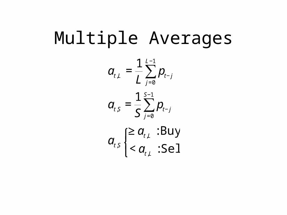
Multiple Averages

€

at ,L =1L

pt− jj=0

L−1

∑

at ,S =1S

pt− jj=0

S−1

∑

at ,S

≥ at ,L : Buy

< at ,L : Sell ⎧ ⎨ ⎩

Bands

€

at ,L =1L

pt− jj=0

L−1

∑

at ,S =1S

pt− jj=0

S−1

∑

at ,S

≥ (1+ B)at ,L : Buy

< (1− B)at ,L : Sell ⎧ ⎨ ⎩

Channel Rule

€

mt−1 = min(pt−L ,K pt−1)

M t−1 = max(pt−L ,K pt−1)

t = Buy

pt

< (1− B)mt−1 : Sell

≥ (1+ B)mt−1 : Buy

Otherwise : neutral

⎧

⎨ ⎪

⎩ ⎪

t = Sell

pt

≤ (1− B)M t−1 : Sell

≥ (1+ B)M t−1 : Buy

Otherwise : neutral

⎧

⎨ ⎪

⎩ ⎪

Channel Rule

€

t = neutral

pt

> (1+ B)M t−1 : Buy

< (1− B)mt−1 : Sell

Otherwise : neutral

⎧

⎨ ⎪

⎩ ⎪

Filter Rule

Buy period to sell Price falls by f fraction from recent price

maxSell period to buy

Price rises by f fraction from recent price min

Rule Evaluation

Statistical significance Breakeven transaction costsRisk

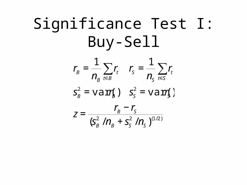
Significance Test I: Buy-Sell

€

r B =1nB

rtt∈B∑ r S =

1nS

rtt∈S∑

sB

2 = var(rB ) sS

2 = var(rS )

z =r B − r S

(sB

2 /nB + sS

2 /nS )(1/2)

Significance Test II: Dynamic strategy, genmatrule.m

€

st =1: Buy

−1: Sell ⎧ ⎨ ⎩

xt = strt

x =1n

xtt=1

n

∑ , s2 = var(x)

z =x

(s2 /n)(1/2)

Probability of a Price Rise

€

p1 = Pr(rt+1 > 0 | t is buy)

p2 = Pr(rt+1 > 0 | t is sell)

p = Pr(rt+1 > 0)

sp1

2 = var(p1) =p(1− p)

nB

sp2

2 = var(p2 ) =p(1− p)

nS

z =p1 − p2

(sp1

2 + sp2

2 )(1/2)z'=

p1 − 0.5(0.25 /nB )(1/2)

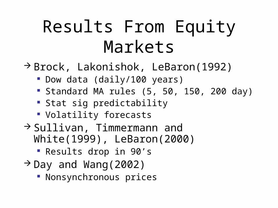
Results From Equity Markets

Brock, Lakonishok, LeBaron(1992) Dow data (daily/100 years) Standard MA rules (5, 50, 150, 200 day) Stat sig predictability Volatility forecasts

Sullivan, Timmermann and White(1999), LeBaron(2000) Results drop in 90’s

Day and Wang(2002) Nonsynchronous prices

Global Equity Markets

Bessembinder and Chen(1995) Repeat results for Asia

Hudson, Dempsey, and Keasey(1996) Long range results form UK

Consistent predictability over many years, many countries

Predictability falling over time

FX Markets

Generally stronger predictability than equity markets Levich and Thomas(1993) LeBaron(1992)

Some connections with intervention LeBaron(1999)

Transaction Costs

Costs of trading: ImportantOften assume proportionalDepends on strategyFirst strategy:

Simple (Long/short) futures Long in buy periods Short in sell periods

Transaction Costs: I. Simple long/short futures

€

PT = (1+ r1' )(1+ r2

' )(1− c)(1− c)(1− r3' )(1− r4

' ) −1

log(1− c) ≈ −c

log(1+ PT ) = r1 + r2 − c − c − r3 − r4

ER = log(1+ PT ) = strtt=1

T

∑ − 2Ntradec

Daily Sharpe ratio =(1/T )ERσ (strt )

Annual Sharpe =(250 /T )(ER)

250σ (strt )

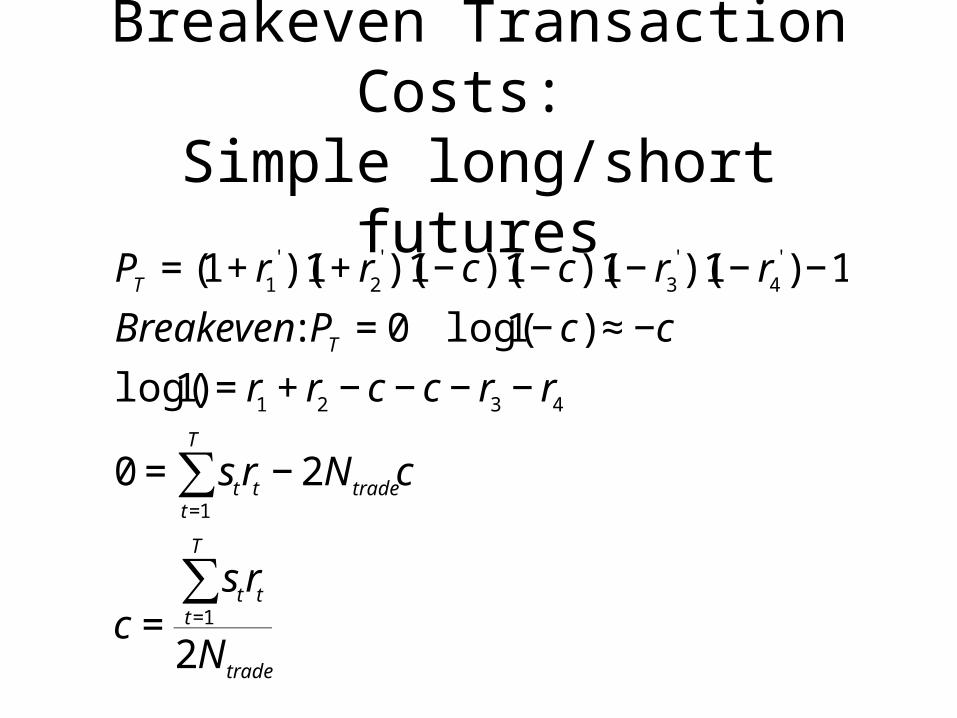
Breakeven Transaction Costs:

Simple long/short futures

€

PT = (1+ r1

' )(1+ r2

' )(1− c)(1− c)(1− r3

' )(1− r4

' ) −1

Breakeven : PT = 0 log(1− c) ≈ −c

log(1) = r1 + r2 − c − c − r3 − r4

0 = strtt=1

T

∑ − 2N tradec

c =strt

t=1

T

∑2N trade

Transaction Costs: Simple Equity Strategy

Equity strategy: Sell: Hold risk free Buy: Leverage position

Invest own $1, borrow additional $1 Designed to replicate risk on buy and hold

Transaction costs: Equity strategy

€

WT = (1 + 2r1' − r ' )(1 + 2r2

' − r ' )K

(1 − c)(1 + r ' )(1 + r ' )

log(WT ) = 2r1 − r + 2r2 − r − c + r + r

Adjust for oportunity cost(excess return)

ER = 2r1 − r + 2r2 − r − c + r + r − 4r

ER = (2rt − 2r)t=1

2

∑ − c

ER = It,B 2(rt

t=1

T

∑ − r) − Ntradec

Sharpe =(1/T )ERσ (ER)

Annual Sharpe =250(1/T )(ER)

250σ (ER)

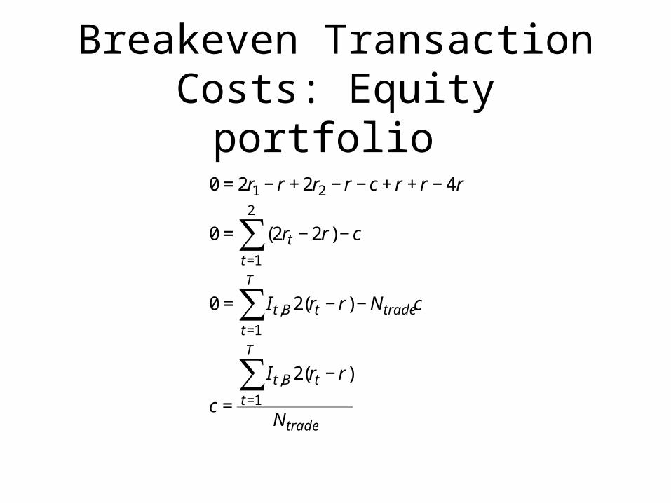
Breakeven Transaction Costs: Equity portfolio

€

0 = 2r1 − r + 2r2 − r − c + r + r − 4r

0 = (2rt − 2r)t=1

2

∑ − c

0 = It,B 2(rt

t=1

T

∑ − r) − Ntradec

c =

It,B 2(rt − r)t=1

T

∑Ntrade

Results

US equity(Dow): 0.22% for recent periods Smaller than most T-cost estimates

Older periods (up to 1%) Currencies: large returns for 0.2% transaction

levels (6-10%) (Sharpe ratios near 1) All near zero beta

Recent Results

All trading rule returns falling in the 1990’s

Increased efficiency?LeBaron(1999): FX interventions

Removing intervention period removes most fx predictability

Few US interventions in the 90’s

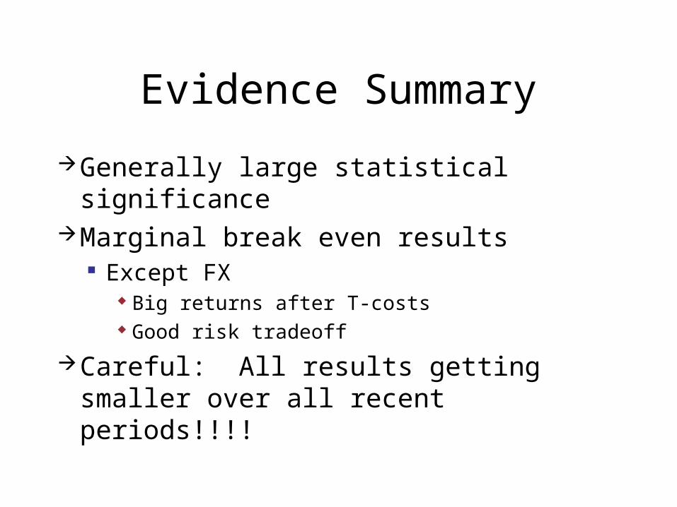
Evidence Summary

Generally large statistical significanceMarginal break even results

Except FX Big returns after T-costs Good risk tradeoff

Careful: All results getting smaller over all recent periods!!!!

Bootstrap Tests

Brock, Lakonishok, and LeBaron(1999) Scrambled returns series

(Monte-carlo: simulated normal returns) Destroy patterns Evaluate rules on scrambled series Compare with original Matlab:

bsmarule.m

Extensions

Fancier rules Better positions Pattern recognition systems

Changing position sizes based on various signals

More advanced risk measures