Trading Bitcoin and Online Time Series Prediction

Muhammad J Amjad mamjad@mit.eduOperations Research CenterMassachusetts Institute of TechnologyCambridge, MA 02139, USA

Devavrat Shah devavrat@mit.eduDepartment of Electrical Engineering and Computer ScienceMassachusetts Institute of TechnologCambridge, MA 02139, USA

Editor: Oren Anava, Marco Cuturi, Azadeh Khaleghi, Vitaly Kuznetsov, Alexander Rakhlin

AbstractGiven live streaming Bitcoin activity, we aim to forecast future Bitcoin prices so as to execute

profitable trades. We show that Bitcoin price data exhibit desirable properties such as stationarityand mixing. Even so, some classical time series prediction methods that exploit this behavior, suchas ARIMA models, produce poor predictions and also lack a probabilistic interpretation. In lightof these limitations, we make two contributions: first, we introduce a theoretical framework forpredicting and trading ternary-state Bitcoin price changes, i.e. increase, decrease or no-change; andsecond, using the framework, we present simple, scalable and real-time algorithms that achieve ahigh return on average Bitcoin investment (e.g. 6-7x, 4-6x and 3-6x return on investments for testsin 2014, 2015 and 2016), while consistently maintaining a high prediction accuracy (> 60-70%) andrespectable Sharpe Ratio (> 2.0). Furthermore, when trained on a period eight months earlier thanthe test period, our algorithms performed nearly as well as they did when trained on recent data!As an important contribution, we provide a justification for why it makes sense to use classificationalgorithms in settings where the underlying time series is stationary and mixing.

1. Introduction

The ubiquity of time series is a fact of modern-day life: from stock market data to social mediainformation; from search-engine metadata to webpage analytics, modern-day data exists as acontinuous flow of information indexed by timestamps. Our focus in this paper is on making scalableand accurate forecasts in real-time, given a live stream of time series data. We specifically considernonparametric time series prediction algorithms, which can adapt to different structure that may bepresent in data across heterogeneous application domains. We anchor our discussion to forecastingBitcoin price changes for algorithmic trading, an application that demands fast, accurate predictions.

1.1 The Problem

Let p[t] be the price of Bitcoin at time t ∈ Z+. We have two main problems of interest:Prediction. For any time t, given the historical price time series up to time t, predict the price forfuture time instances, s ≥ t+ 1.Trading. For any time t, using current investment and predictions, decide whether to buy newBitcoins or sell any of the Bitcoins that are in possession.

Our work focuses on the problem of predictions and the purpose of a trading strategy is todemonstrate the utility of accurate predictions. For this reason, we consider an extremely simpletrading strategy which shall be simulated under idealized conditions which ignore volume effectsand transaction costs. Accordingly, we limit the number of Bitcoins that can simultaneously be

1

possessed to one. Formally, at time t, let h[t] = 1, if we are in possession of a Bitcoin and h[t] = 0,otherwise. Given h[t] and a prediction of whether the price will go up, down, or stay about the same,the decision d[t] at time t is given by:

d[t] =

buy, if h[t] = 0 & price is predicted to increase, with high confidencesell, if h[t] = 1 & price is predicted to decrease, with high confidencehold, otherwise.

Effectively, we have a decision-making exercise relying on a prediction of the future. Therefore, itis desirable for there to be a quantification of the confidence for each prediction such that the tradingalgorithm can shield itself from low-confidence predictions.

1.2 Our Contribution

Our main contributions are two-fold: we develop a theoretical framework for time series analysisbased on reasonably generic properties of a time series, namely stationarity and mixing; and second,we present simple, scalable, real-time algorithms for prediction and trading that yield high predictionaccuracy and highly profitable returns on investment in Bitcoin.

A time series being stationary means that its joint probability distribution is time-invariant.Mixing means that the distribution at a specific time is primarily dependent on the recent past. Bothhold for a discrete time series tracking the first-differences of Bitcoin prices, as we show in Section2.2 using the Dickey-Fuller and the Kwiatkowski-Phillips-Schmidt-Shin tests (stationarity) and theAutocorrelation Function (ACF)/ Partial Autocorrelation Function (PACF) plots (mixing). Thus,classical time series regression algorithms, e.g. ARIMA, that exploit stationarity and mixing could beused to forecast price changes, yet as we show in Section 2.3, they have poor prediction performance.They also lack a probabilistic interpretation that make them even less attractive options to be usedin conjunction with a trading strategy which would benefit from shielding itself from low-confidencepredictions.

To overcome these limitations, we propose a model for forecasting the price change, i.e. increase,decrease, or no change, that relies on stationarity and mixing (Section 2.5). Effectively, we argue thatfor such time series, the probability distribution of the future prices, {increase, decrease, no-change},is a continuous function of the recent past that can be approximated from finite data. With thisinsight, we present a collection of algorithms that estimate this conditional probability distribution:classification algorithms like Random Forest, Logistic Regression and LDA; and an algorithm thatexplicitly learns the empirical conditional probability distribution from data. Effectively, we providea justification, rooted in first principles, that allows classification algorithms to be effective in suchsettings–a crucial link missing in related works. The performance of the resulting algorithms issummarized next (details in Section 3.4):Algorithm Comparison. Our proposed algorithms return several multiples of investment acrossall tests, e.g. a 6-7x return on investment over a two month test period in 2014, a 4-6x return overtwo months in 2015 and 3-6x return over 4 months in 2016, while consistently maintaining a 60-70%accuracy and a Sharpe Ratio (Sharpe, 1998) over 2.0. In comparison, ARIMA based predictionsusually performed poorly across all metrics.Sensitivity. We choose a training period eight months earlier than the testing period and noticethat while ARIMA loses money consistently, our algorithms perform nearly as well as they do whentrained on more recent data, producing a 4-6x return on investment with a ∼ 60-70% accuracy. Thispoints to the incredible robustness of our approach and fragility of ARIMA. Additionally, we canachieve greater robustness by considering a set of the lengths of history, instead of single length d.Stability. We use the Sharpe Ratio to understand how consistent the trading strategy (Maverick,2015) is. Our algorithms yield a Sharpe ratio consistently near or above 2.0, which is considered verygood, while ARIMA lags far behind, at times < 0.

2

1.3 Related Works

There are two sets of literatures related to our work: financial and time series data analysis. Infinancial literature, one of the relevant approaches is technical analysis, which assumes that pricemovements follow a set of patterns and one can use past price movements to predict future returns(Lo and MacKinlay, 1988, 1999). Caginalp and Balenovich showed that some patterns emerge froma model involving two distinct groups of traders with different assessments of valuation (Caginalpand Balenovich, 2003). Some empirically developed geometric patterns, such as heads-and-shoulders,triangle, and double-top-and-bottom, can be used to predict future price changes (Lo et al., 2000;Caginalp and Laurent, 1988; Park and Irwin, 2004). In particular, in (Lo et al., 2000) authors utilizethe method of Kernel regression to identify various geometric patterns in the historical data. Priceis predicted using recent history. In that sense, (Lo et al., 2000) is closest to this work. However,we note that (Lo et al., 2000) does not yield any meaningful prediction method or for that mattereventually yield a profitable trading strategy. Our work, given the above literature, can be viewed asan algorithmic version of the “art of technical trading”.

In the context of time series analysis, classical methods are a popular choice. For example, theARIMA models which tend to capture non-stationary components through finite degree polynomials;or using spectral methods to capture periodic aspects in data, described in detail in works such as(Brockwell and Davis, 2013; Hamilton, 1994; Robert H. Shumway, 2015). In contrast, our approachis nonparametric and stems from a theoretical modeling framework based on stationarity and mixing.A natural precursor to this work are (Chen et al., 2013) and (Shah and Zhang, 2014), where thenonparametric classification has been utilized for predicting trends. Classification algorithms havebeen used to predict stock price changes previously, e.g. Ch. 4.6.1 of (James et al., 2013), (Gong andSun, 2009), (Alrasheedi and Alghamdi, 2012). However, none of these works provide a theoreticalframework justifying why these algorithms are suited for this problem space. Additionally, they tendto operate on a daily, weekly or monthly time-resolution which is in contrast to our goal of nearreal-time predictions.

2. Modeling Bitcoin Time Series

We now describe the Bitcoin data and establish stationarity and mixing. Next, we show that theclassical modeling approach comes up short. Subsequently, we describe a modeling framework thatholds promise in this setting and end by presenting our model and algorithms that fit the framework.

2.1 Bitcoin Data

We are using Bitcoin data, accessed via the OKCoin exchange using their APIs okc. All prices arereported in Chinese Yuans. The APIs return lists of bid[t] and ask[t] prices at the exchange, whichare the list of prices that buyers are willing to pay, and the list of prices that sellers are demanding(for one Bitcoin), respectively at time t. We cached several months of data from the exchange in2014, 2015 and 2016. Therefore, the experiments in this work are reported for those periods. Atevery point in time, t, we create an estimate of price as, p[t] = (max(bid[t]) + min(ask[t]))/2. Hence,the pair (t, p[t]) represents a time series of Bitcoin price estimates. As an example, refer to Figure 1(Left) for the Bitcoin price time series during a four month period in 2014.

2.2 Stationarity and Mixing

Given that the classical modeling approaches assume stationarity, we check for it using the AugmentedDickey-Fuller (DF) Test (Said and Dickey, 1984) and the Kwiatkowski-Phillips-Schmidt-Shin (KPSS)test (Kwiatkowski et al., 1992). Both are hypothesis tests where DF assumes non-stationarity as thenull hypothesis while KPSS assumes the opposite. They reveal that the Bitcoin price time seriesis not stationary (p-value > 0.3 for DF; p-value < 0.01 for KPSS). However, as is often observed

3

Figure 1: Left: Price of Bitcoin in Chinese Yuan from 12/1/2014 to 3/31/2015. Center: A histogram offirst-differences of the price time series that is sampled every 5 seconds. Right: A QQ-plot against a Gaussian(0.02, 0.04).

Figure 2: Left: ACF plot for the Bitcoin price time series, sampled at 10s. This implies q ≤ 8. Center:PACF plot for the Bitcoin price time series, sampled at 10s. This implies p ≤ 8. Note: a value of 10s on thex-axis implies a lag = 1. Right: ARIMA (4,1,4) predictions with actual series, showing 50 data points.

with econometric data, the time series produced by the first-differences, i.e. y[t] = p[t]− p[t− 1], isstationary (p-value < 0.01 for DF; p-value > 0.1 for KPSS). Figure 1 (Center) shows the histogram ofthe first-differences of the Bitcoin price time series, sampled at 5s intervals, and the QQ-plot (Right)confirms that the data appears to follow a Gaussian distribution. Additionally, the Kolmogorov-Smirnov test fails to reject the hypothesis that the first-differences follow a zero-mean Gaussianmarginal distribution, thereby confirming stationarity.

We find that y[t] is a mixing process. Recall that a stochastic process is mixing if its valuesat widely-separated times are asymptotically independent (Shalizi, 2007). The AutocorrelationFunction (ACF) and Partial Autocorrelation Function (PACF) plots in Figure 2 (Left, Center) showexponential decay, implying mixing.

In summary, based on the outcomes of all the tests it is safe to conclude that the first-differencesof the Bitcoin price time series is stationary and mixing.

2.3 Classical Modeling: ARIMA

A natural reference point in time series modeling is to consider the classical techniques like the ARIMAmodels. Their effectiveness in understanding and predicting time series data such as weather forecasts(Mahmudur Rahman and Rahman, 2013), sales of electricity (Ugiliweneza, 2007), unemploymentrates (Dobra and Alexandru, 2008) and for other econometric problems (Asteriou, 2016) have beenwell documented. Thus, we try to understand how well they work in our setting.

In order to fit an ARIMA model, which assumes stationarity, we need to use our data to determinethe three parameters: p, d, q. p corresponds to the autoregressive component, q to the moving-average and d is the degree of differencing Box and Reinsel (1994); Robert H. Shumway (2015). TheDickey-Fuller and KPSS tests have already revealed that d > 0 for stationarity. Using the ACF and

4

PACF plots in Figure 2 (Left, Center) as our guides, we can safely assume that p, q ≤ 8. The lowestAIC/BIC values for the best fit were given by (p, d, q) = {4, 1, 4} and (p, d, q) = {2, 1, 1}.

Figure 2 (Right) shows the point-predictions using ARIMA(4,1,4). The model is updated usingeach new data point and predictions are shown in the plot. The plots are zoomed in to show ahandful of points to underscore how the predictions tend to be nearly one-step shifted versions of theoriginal. This does not appear very promising given that all predictions are approximately trackingthe latest data point in the past, providing little new information. Additionally, they do not providea probability for each prediction. This can potentially be a severe handicap when coupled with atrading strategy that could benefit from a probabilistic framework for deciding the confidence withwhich it can commit to new trades.

2.4 Back to First Principles

Given that the first-differences of Bitcoin price time series, y[·], is stationary and mixing, it suggeststhat there exists a large enough d ∈ Z+ so that

P(y[t]|y[−∞ : t− 1]) ≈ P(y[t]|y[t− d : t− 1]), (1)

where y[a− d : a] = (y[a− d], . . . , y[a]) for any a ∈ Z, d ≥ 1. (1) states that the distribution of y[t],conditioned on a finite but long enough history, is approximately the same as that for the samplewith entire past. Additionally, since y[t] is stationary, we have:

P(y[t]|y[t− d : t− 1]) ≈ P(y[s]|y[s− d : s− 1]),∀s. (2)

This is a critical observation because it leads us to conclude that for two entirely disparate points intime if the finite-length history is similar then the process’ probabilistic evolution in the future willalso be similar.

From (1) and (2), a reasonable approximation for the y[·] process is a Markov Chain with statez[·], where z[t] ≡ y[t − d : t], and the state transition probability is a measurable function fromRd+1 → R with respect to Borel σ-algebra (cf. see Ch. 6 of Durrett (2010), for precise definition).That is, for any given θ ∈ R, consider function Fθ : Rd → [0, 1] defined as

Fθ(y[t− d : t− 1]) = P(y[t] > θ|y[t− d : t− 1]), (3)

for any t ∈ Z (recall, Fθ does not depend on t as it is a stationary process). This is a measurablefunction. A special class of measurable functions (which is quite general) is the space of continuousfunctions. We shall assume that our class of model satisfies this restriction.

Key Model Assumption. For any θ ∈ R, Fθ as defined above is a continuous function.

2.5 Our Model

Given θ ∈ R, define

x[t] =

−1, if y[t] < −θ1, if y[t] > θ

0, otherwise.(4)

Given history length d ≥ 1, define a 3-dimensional probability vector Q[t] = (P(x[t] = σ|y[t − d :t− 1]), σ ∈ {−1, 0, 1}). Then we posit that Q[t] = F (y[t− d : t− 1]), for some continuous functionF : Rd → [0, 1]3 for all t ∈ Z. This directly follows from our model assumption.

We note that our interest is truly in this 3-dimensional vector since we are interested in tradingBitcoins, and the future decision in the simple trading strategy is primarily determined by whetherprices are going to go up, down or remain approximately the same. In general, for other decisionmaking tasks, one might be interested in more or less detailed aspects of the distribution of futureprices.

5

2.5.1 Prediction Algorithm using Classification

Given the model, the problem effectively reduces to ternary-state classification. In particular, wecan generate training data as follows: (x[t], y[t− d : t− 1]) for each t provides a sample to train themodel. This, when coupled with any classification algorithm, provides an algorithm for the purpose ofprediction. Classification algorithms afford a significant additional advantage: they can incorporate aricher feature set. For our classification algorithms we perform an initial "feature extraction" basedon y[: t− 1]. Recalling that x[t] is calculated from y[t], y[t− 1] as defined in Equation 4, we extractthe following features:

1. x[t− 1]: the latest change in price. This captures the most recent movement in price.

2. Tσ,d[t− 1] =∑t−1s=t−d 1{x[s] = σ}: the tally-count of each quantized value in x[t− d : t− 1], for

every d and σ ∈ {−1, 0, 1}. This tally-count feature allows us to capture the recent distributionof price-changes which provides more information than that contained in the first feature above[1].

3. Cσ[t− 1] = maxk(k : σ = x[t− 1] = x[t− 2] = · · · = x[t− k]): consecutive run-length of eachquantized value σ ∈ {−1, 0, 1}. This feature allows us to capture trends of consecutive rises,falls and no-changes in the price process leading up to the current point in time.

This collection of features allows us to capture information leading up to the current point intime, ∀t. Features 2 and 3 allow us to capture a richer amount of information compared to they[t − d : t − 1] being used by ARIMA models. Intuitively, we expect a richer feature set to allowthese classification algorithms to perform better than ARIMA models which simply consider the pastprices as a single "feature".

Effectively, for classification algorithms we have Q[t] = F (y[t− 1], Tσ,d[t− 1], Cσ[t− 1]) and F (·) isbelieved to have "simple" structure. The goal is to learn F (·) ∈ [0, 1], using a classification algorithm.

Connections and Contrast with Prior Work. Predicting quantized prices by using classificationalgorithms has been tried previously, e.g. Ch. 4.6.1 of James et al. (2013), Gong and Sun (2009),Alrasheedi and Alghamdi (2012). However, our work goes beyond the simple application of algorithmsand directly ties the efficacy of these algorithms to the general modeling framework which assumesstationarity and mixing. Additionally, unlike past works, we do not restrict ourselves to predictionalone; we couple it with a trading strategy. Furthermore, the scale of Bitcoin data at our disposalprovides a better stress test of these classification algorithms at a low latency, e.g. 5-10s, in contrastto daily, weekly or monthly resolutions considered in prior works.

Which Classification Algorithms to use? For our choice of classification algorithms, we turnto Random Forest (RF), Logistic Regression (LR) and Linear Discriminant Analysis (LDA). Forthe Bitcoin time series, they carry promise because they attempt to learn the transition probabilitydistribution function, P(x[t]|hd[t]) given input data, and hence, satisfy the general framework. Theyare also known to be efficient, scalable and robust.

2.5.2 Approximate Empirical Conditional (EC) Distribution

Another approach is to learn the actual conditional distribution, exactly. Of course, this is notfeasible given a continuous state-space and limited data, so we quantize the state-space to produce areasonable approximation. Specifically, we can learn the approximate distribution by consideringthe empirical conditional (EC) distribution of x[·] given d-step history, hd ≡ x[t − d : t − 1]. Fora fixed d ≥ 1, σ ∈ {−1, 0, 1} and hd ∈ {−1, 0, 1}d, the EC distribution of interest, is denoted byPd(σ|hd). See Appendix A for a precise definition. We can build these probability maps for eachprefix, hd, and that is effectively the model. Note that this model relies only on the past d valuescorresponding to each data point making it more comparable to ARIMA models. This also suggests

6

that due to the availability of only finite amount of data, learning the empirical distribution willlikely be outperformed by the classification algorithms which have the advantage of incorporating aricher feature set, as discussed earlier.

2.5.3 Prediction Probabilities, Thresholds and Risk Profile

Our algorithms produce a prediction for each step in the future. At time t − 1, the prediction isx̂[t] ∈ {−1, 0, 1} for the next time step. However, we require the model to produce a probabilityassociated with each prediction to give us a sense of confidence in each individual prediction. This isuseful because it can help the trading strategy avoid committing to trade-decisions for low-confidencepredictions. Specifically, we produce 0′s for all predictions below a tunable confidence threshold:

x̂[t] =

{σ∗ if P∗(x[t] = σ∗|hd[t− 1]) ≥ γ,0, otherwise,

(5)

where σ∗ = argmaxσ∈{−1,0,1} P(x[t] = σ|hd[t− 1]).The use of γ is to threshold the quality of the estimator. If the estimator is not confident enough,

then we ignore the prediction and predict 0. In the context of trading algorithm, this means thatit does nothing, i.e. it performs no trades. That is, when the signal is not strong enough as perprediction algorithm, the trading algorithm does not decide to make bets either way. Additionally, γis the only customization parameter of the entire system. It can be chosen to suit the risk profile.For example, a low value of γ such as 0.5, would mean that we produce predictions that are morelikely to be incorrect on new data. On the other hand, a very high γ, say 0.9, might result in few orno trades.

We use a validation set to determine the best γ for our tests. Given the inverse relationshipbetween accuracy and number of trades, we choose the γ value that maximizes the product ofaccuracy and profit on the validation sets. This approach allows us to choose γ in a manner thatpenalizes both high accuracy with low expected profit and low accuracy with high expected profit.

Combining Multiple Predictions. For the EC model (Section 2.5.2), suppose we use a set ofvalues of d ≥ 1, denoted as S. For each d ∈ S, let x̂d[t] be the prediction obtained for time t basedon history hd as discussed above. We produce a weighted combination of these predictions, denotedas x̂w[t]:

x̂w[t] =∑d∈S

x̂d[t]× wd, where∑d∈S

wd = 1. (6)

One suggested way of computing the weights, wd, is detailed in Appendix B, using information-theoretic ideas. Finally, we further quantize x̂w[t] to produce our prediction x̂[t] ∈ {−1, 0, 1}, similarlyto the discretization described in Section 2.5.

3. Experiments and Results

3.1 Experimental Setting

We conducted several experiments to evaluate the predictions produced by all algorithms discussedearlier. The experiments were simulated using the OkCoin data from 2014, 2015 and 2016. γ waschosen using a validation set, unless noted otherwise. d was typically chosen from among {3,4,5}.Lastly, we fixed the price sampling rate to 5s and θ = 0.

3.2 Objectives

The primary objective of our experiments is to compare our prediction algorithms with ARIMAas a baseline. Additionally, we want to study the sensitivity of and trade-offs introduced by the

7

Figure 3: Cumulative Profit and Bitcoin Price in 2014, 2015, 2016 with d ∈ 3, 4, 5. γ selected via validation.Each time step represents 5s.(Left): Training: 2/16/14 - 3/14/14, Validation: 3/15/14 - 3/31/14, Test: 4/1/14 - 6/11/14.(Center): Training: 12/1/14 - 12/31/14, Validation: 1/1/15 - 1/15/15, Test: 1/16/15 - 3/31/15.(Right): Training: 2/26/16 - 4/15/16, Validation: 4/16/16 - 5/15/16, Test: 5/16/16 - 9/15/16.

model parameters, e.g. d, γ. Performance sensitivity to the choice of training periods is anotherobjective of evaluation. Finally, the experiments must also enable us to gauge the stability of thealgorithms vis-a-vis the trading strategy.

3.3 Evaluation Criteria

We use the following metrics for evaluating the performance of all models under consideration:Prediction Accuracy. Foremost, our priority is to evaluate the accuracy of the predictions producedby each algorithm. Our accuracy measure is simply the proportion of predictions we get correct fromamong the {-1, 1} predictions we make. Note that this means we ignore evaluating the accuracywhen x̂[t] = 0 because our trading strategy ignores them. For m predictions, starting at time t:

Accuracy =

∑m−1j=0 1{x̂[t+ j] = x[t+ j]}1{x̂[t+ j] 6= 0}∑m

j=1 1{x̂[t+ j] 6= 0}(7)

Cumulative Profit. Given that we are simulating a trading strategy for Bitcoin, the most naturalmetric for evaluation is the cumulative profit across the period of execution.Investment Returns. Simply reporting cumulative profit can hide an important factor in theevaluation of a trading strategy: the investment required to achieve the profit or returns. We alsoreport the profit as a ratio of the average investment required during the period of the experiment.Sharpe Ratio. We use the Sharpe Ratio to quantify how well (or worse) the policy does comparedto the risk-free returns and with how much volatility. A Sharpe Ratio in excess of 1.0 should beconsidered pretty good, greater than 2.0 is considered great and so on. In our case we define oneperiod of trading to be the equivalent of a month. Please see Appendix C for details on how wecalculate it.

3.4 Results

Compare Algorithms. The standout conclusion is that the classification algorithms outperformboth EC and ARIMA on all metrics. Refer to Figure 3 and Table 1, Table 5 (Appendix E) and Table6 (Appendix E) for the experiments in 2014, 2015 and 2016. They generated approximately 4-6x inreturns, with a Sharpe Ratio over 2.6 and accuracy over 70% in results for the 45 day test periodin 2015. For the experiment in 2014, they generated approximately 7x return with Sharpe Ratioover 2.5 with an accuracy > 65%. For this problem space, a 70% accuracy is great, as discussed in

8

Figure 4: Comparison of the cumulative Profit for the same Test period in 2015 with a recent trainingperiod and an eight month old training period. d ∈ 3, 4, 5 and γ selected on the same validation set. Eachtime step represents 5s.(Left): Training: 12/1/14 - 12/31/14, Validation: 1/1/15 - 1/15/15, Test: 1/16/15 - 3/31/15.(Right): Training: 2/16/14 - 3/14/14, Validation: 1/1/15 - 1/15/15, Test: 1/16/15 - 3/31/15.

Profit Return Sharpe Accu.

Arima 1366.7 0.9 0.43 0.49EC 5721.1 3.7 2.17 0.64RF 6049.9 3.9 2.56 0.78LDA 7469.0 4.8 2.82 0.73LR 9090.9 5.9 3.32 0.70

Table 1: Using a recent training period. Train-ing: 12/1/14 - 12/31/14, Validation: 1/1/15 -1/15/15, Test: 1/16/15 - 3/31/15. d ∈ 3, 4, 5; γis selected via validation.

Profit Return Sharpe Accu.

Arima -4758.5 -3.1 -2.0 0.43EC 5721.4 3.7 2.2 0.64RF 7903.1 5.1 3.4 0.69LR 8019.4 5.2 3.5 0.71LDA 7934.1 5.1 3.3 0.69

Table 2: Using an eight month old Trainingperiod, same validation and test periods as thosein Table 1. Training: 2/16/14 - 3/14/14. d ∈3, 4, 5; γ is selected via validation.

Ch. 4.6.1 of James et al. (2013). Among the classification models, all choices under considerationperform comparably. This is a significant result because it establishes the efficacy and robustnessof the classification algorithms for time series modeling while conforming it to a general modelingframework constructed from first principles.

EC tends to fare much better than ARIMA models, e.g. over the 2.5 months in the test period in2014 (Left plot), a return of 5.7x with Sharpe Ratio of 1.62 compared to a 3.2x return and 1.6 SharpeRatio of the ARIMA mode. For the test in 2015, EC generates a 3.7x return with Sharpe of 2.2compared to ARIMA generating 0.9x return with Sharpe of 0.43. This trend extends to predictionaccuracy as well. During the test period in 2016, ARIMA and EC perform comparably (refer toFigure 3). Under most circumstances, ARIMA performs poorly on all metrics. The parameters usedin these experiments, p = 4, d = 1, q = 4, were determined using cross-validation on the training set.

Sensitivity: Training Period. Refer to Figure 4 (Right) and Table 2 . Even though there is a lagof about eight months between the training and testing periods, EC and all classification algorithmscontinue perform very well, while ARIMA loses money consistently. This incredible finding showsthat patterns of historical evolution of y[t] repeat fairly often and are observed frequently across longperiods of time and are captured well by EC and classification algorithms.

Sensitivity: Single vs Multiple d. Table 3 shows the noticeable robustness introduced by usingmultiple d values instead of just one. When using d ∈ {3, 4, 5} instead of just using one, we noticethat the cumulative profits and accuracy are better or, at least, no worse than those produced by

9

RF ECd Profit Accu. Profit Accu.

3 8555.5 0.78 9082.5 0.654 8545.7 0.78 8248.6 0.635 8604.8 0.79 7114.4 0.653,4,5 8624.9 0.79 9091.4 0.65

Table 3: Effects of choosing multiple valuesof d. γ = 0.65 is fixed and no validation isused. Training Period: 12/1/14 - 1/1/15; TestPeriod: 1/1/15 - 3/31/15. Only showing RFand EC.

RF ECγ # Trades Accu. # Trades Accu.

0.60 18634 0.69 25780 0.580.65 9982 0.73 19312 0.600.70 4262 0.77 17190 0.620.75 2230 0.81 6216 0.68

Table 4: Tension between the number of Tradesand Accuracy shown by varying γ is varying (novalidation) with d ∈ 3, 4, 5 fixed; Training Period:12/1/14 - 1/1/15; Test Period: 1/1/15 - 3/31/15.Only showing RF and EC.

choosing single values of d. Note that for this experiment γ was fixed to showcase the effect ofchoosing single vs multiple values of d.

Trade-Off: Accuracy vs # Trades. As discussed in Section 2.5.3, the choice of γ determines therisk-profile of the trading algorithm. γ should be chosen via cross-validation or simply by tuning iton a validation set like we do for our experiments discussed earlier. However, in order to confirmour intuition about the tradeoffs between accuracy and number of trades (which influences profits),we conducted some experiments by keeping d fixed and varied γ. We can see from the results inTable 4 for EC and RF, the higher we set γ the greater our accuracy. However, the higher the γ thelower the resulting number of trades because a higher γ also means more predictions of 0 resulting infewer trades. This confirms the tension between more/less trades and smaller/greater accuracy weintuitively expected.

Stability: Sharpe Ratio. Tables 1, Table 2, Table 5 (Appendix E) and Table 6 (Appendix E)show the Sharpe Ratio for all algorithms. ARIMA does not perform as well as the others. Theclassification algorithms and EC consistently manage a Sharpe Ratio near or in excess of 2.0 whichshould be considered a very good indicator of the over all stability of the trading scheme during theentire testing period spanning several months.

4. Conclusion

After establishing the appropriate learning framework, we first indicate the limitations of classicaltime series methods like the ARIMA models. Next, we build a general modeling framework from firstprinciples which is expected to work well in this setting. We discuss two approaches that conform tothe framework: Classification algorithms and directly learning the empirical conditional distribution(EC). They all outperform ARIMA on all evaluation metrics, with classification algorithms performingthe best on experiments spanning 2014-2016. Our results establish that we can achieve a Sharpe Ratioover 2.0 with consistency, and maintain a prediction accuracy near or above 70% while generatingseveral multiples of average investment as return over tests each spanning 2-4 months. For a discussionon a few significant issues not considered in this work, please see Appendix D.

ReferencesOkcoin api. https://www.okcoin.com/about/publicApi.do.

M. Alrasheedi and A. Alghamdi. Predicting up/down direction using linear discriminant analysis and logitmodel: The case of sabic price index. Research Journal of Business Management 6, pages 121–133, 2012.

Stephen G. Asteriou, Dimitros; Hall. Applied Econometrics (Ch 13: . ARIMA Models and the Box–JenkinsMethodology). Palgrave Macmillan, 3rd edition, 2016.

10

Mayank Bawa, Tyson Condie, and Prasanna Ganesan. Lsh forest: self-tuning indexes for similarity search.In International World Wide Web Conference, 2005.

Jenkins Box and Reinsel. Time Series Analysis, Forecasting and Control. Prentice Hall, Englewood Clifs, NJ,3rd edition, 1994.

Peter J Brockwell and Richard A Davis. Time series: theory and methods. Springer Science & BusinessMedia, 2013.

Gunduz Caginalp and Donald Balenovich. A theoretical foundation for technical analysis. Journal of TechnicalAnalysis, 2003.

Gunduz Caginalp and Henry Laurent. The predictive power of price patterns. Applied Mathematical Finance,5:181–206, 1988.

George H. Chen, Stanislav Nikolov, and Devavrat Shah. A latent source model for nonparametric time seriesclassification. In Advances in Neural Information Processing Systems, 2013.

Ion Dobra and Adriana AnaMaria Alexandru. Modelling unemployment rate using box-jenkins procedure.Journal of Applied Quantitative Methods, 2008.

Rick Durrett. Probability: Theory and Examples. Cambridge University Press, 4.1 edition, 2010.

Jibing Gong and Shengtao Sun. A new approach of stock price trend prediction based on logistic regressionmodel. IEEE International Conference on New Trends in Information and Service Science. NISS ’09.,pages 1366–1371, 2009.

James Douglas Hamilton. Time series analysis, volume 2. Princeton university press Princeton, 1994.

Gareth James, Daniella Witten, Trevor Hastie, and Robert Tibshirani. An Introduction to Statistical Learning.Springer, 2013.

D. Kwiatkowski, P. C. B. Phillips, P. Schmidt, and Y. Shin. Testing the null hypothesis of stationarityagainst the alternative of a unit root. Journal of Econometrics, pages 159–178, 1992.

Andrew W. Lo and A. Craig MacKinlay. Stock market prices do not follow random walks: Evidence from asimple specification test. Review of Financial Studies, 1:41–66, 1988.

Andrew W. Lo and A. Craig MacKinlay. A Non-Random Walk Down Wall Street. Princeton UniversityPress, Princeton, NJ, 1999.

Andrew W. Lo, H. Mamaysky, and J. Wang. Foundations of technical analysis: Computational algorithms,statistical inference, and empirical implementation. Journal of Finance, 4, 2000.

Shah Yaser Maqnoon Nadvi Mahmudur Rahman, A.H.M. Saiful Islam and Rashedur M Rahman. Comparativestudy of anfis and arima model for weather forecasting in dhaka. Onternational Conference on Informatics,Electronics and Vision (ICIEV), 2013.

J.B. Maverick. What is a good sharpe ratio. http://www.investopedia.com/ask/answers/010815/what-good-sharpe-ratio.asp, 2015.

Cheol-Ho Park and Scott H. Irwin. The profitability of technical analysis: A review. AgMAS Project ResearchReport No. 2004-04, 2004.

Rajesh Motwani Piotr Indyk. Approximate nearest neighbors: Towards removing the curse of dimensionality.In STOC ’98 Proceedings of the thirtieth annual ACM symposium on Theory of computing. ACM, 1999.

David S. Stoffer Robert H. Shumway. Time Series Analysis and It’s Applications. Blue Printing, 3rd edition,2015.

S. E. Said and D. A. Dickey. Testing for unit roots in autoregressive-moving average models of unknownorder. Biometrica, 1984.

11

Scikit-Learn. Lsh forest implementation.

Devavrat Shah and Kang Zhang. Bayesian regression and bitcoin. CoRR, 2014.

Cosma Shalizi. Lecture Notes on Stochastic Processes (Advanced Probability II). (unpublished),http://www.stat.cmu.edu/ cshalizi/754/notes/all.pdf, 2007.

William F Sharpe. The sharpe ratio. Streetwise–the Best of the Journal of Portfolio Management, pages169–185, 1998.

Beatrice Ugiliweneza. User of arima time series and regressors to forecast the sale of electricity. SESUGProceedings, 2007.

12

AppendicesA. Empirical Conditional (EC) Distribution: Model

Given d ≥ 1, the EC distribution of interest, is defined as follows: for any σ ∈ {−1, 0, 1} and anyhd ∈ {−1, 0, 1}d,

Pd(σ|hd) =Nd((σ,hd))∑

γ∈{−1,0,1}Nd(γ,hd), (8)

where Nd((σ,h) = |{t : x[t] = σ, x[t− d : t− 1] = hd[t− 1]}| given data x[·].This is effectively an exercise is creating discrete-space probability maps, learned from data by

counting the occurrences of specific prefixes, hd ∈ {−1, 0, 1}d followed by each x[t] = σ = {−1, 0, 1}.

B. Empirical Conditional (EC) Distribution: Prediction with Multipled ≥ 1.

We produce a ‘weighted’ combination of predictions, denoted as x̂w[t]:

x̂w[t] =∑d∈S

x̂d[t](wd) (9)

where, wd = (1− Id(hd))Qd(hd). We borrow from Information-theoretic ideas and let Id denote theamount of Information contained for a given d; Qd(hd[t]) simply denotes the fraction of times aparticular prefix, hd[t], is observed. More formally, we first compute the conditional entropy:

H(hd) = −∑

σ∈{−1,0,1}

Pd(σ|hd) log3 Pd(σ|hd). (10)

Let Nd(h) = |{t : x[t− d : t− 1] = h}| be the number of times hd is d-step prefix. Then, we have:

Q(hd) =Nd(hd)∑

gd∈{−1,0,1}d Nd(gd). (11)

In above, we use notation 0/0 = 0. We then denote the information content in the sequence by:

Id =∑

hd∈{−1,0,1}dQ(hd)H(hd) =

∑hd∈{−1,0,1}d

Id(hd), (12)

C. Sharpe Ratio

We compute the Sharpe ratio of the trading strategy. To recall, the Sharpe ratio of a strategy canbe computed as follows: over N periods, let profiti be the profit (or loss) made in the ith period1 ≤ i ≤ N . Let p0 and pN be the price of the Bitcoin at the beginning and at the end of this interval(i.e. N periods). Then, Sharpe ratio is defined as:

Sharpe Ratio =1N

∑Ni=1 profiti − |p0 − pN |

1N

∑i profit2i − [ 1N

(∑Ni=1 profiti)]

2(13)

13

D. Discussion: Issues not considered

We now comment on a few significant issues not considered in this work:

Scaling of Trading strategy. As noted in Section 1.1, our simple trading strategy is a proof-of-concept trading strategy simulated under idealized conditions. This trading strategy only trades 1Bitcoin and this helps avoid two major issues. Firstly, there is no question of any technical constraintsor exchange-based restrictions to consider as we never trade more than a single Bitcoin. An actualtrading scheme would have to consider the impact of restrictions when thinking of trading moreBitcoins or deciding to short Bitcoins before owning them. Secondly, we avoid considering the impactof our own trading decisions on the equilibrium of the market. Such a simplification can safely bemade when dealing with just a solitary Bitcoin. However, when increasing the quantities of Bitcoinwe decide to trade, one has to develop an understanding of how one’s trading decisions potentiallyimpact the market.

Latency to Exchange. In our work, we have performed trade simulations to evaluate our predictionalgorithm. While our predictions can be used in a real-time trading scheme, there are some importantinfrastructural challenges to consider. Foremost is the latency between placing orders on an exchangeand the fulfillment of that order. Given that we were sampling our pricing data fairly frequently(5s intervals), ensuring that decisions can be made and executed in near real-time is not an trivialtask and is a function of infrastructural limitations of the exchange and the network in between theexchange the the client.

How Large should d be? An important question is how large should d be? Given d, the number ofprefixes scale as 3d. Therefore, with large d, the the data may not be sufficient to provide useful proxyfor empirical distribution. On the other hand, if d is too small, the history may not be informativeenough for the purpose of prediction. Therefore, it is important to use the right compromise choicefor d. One such rule is to keep d ≤ log3(T/100) when T time units of data is available. Based on ourexperiments, this allows for sufficient data for making meaningful empirical estimation.

Computational Complexity of the Model Index. Given that the storage of our prefixes scalesas 3d, if d becomes large, e.g. d > 20, the growth constraints on memory start to become majorhurdles. Even though d should remain small for reasonably large historical pricing information (seethe paragraph above), it is worth considering the approach one might take to overcome the challengesposed by large d. One approximate solution is to build the storage index more cleverly, such as usingLocality Sensitive Hashing (LSH) as proposed in Bawa et al. (2005). The crux of the the work onLSH trees is to find clever hash maps that enable a compressed index which guarantees with highprobability that for ε > 0, if we wish to find k neighbors, such that the distance from a new point qto the i− th nearest neighbor is at most (1 + ε) times the distance from q to its true i− th nearestneighbor’ Piotr Indyk (1999). In essence, LSH trees can replace the index/dictionaries we use tostore the empirical conditional probabilities for our model. These LSH trees can then can produceapproximate nearest neighbors of a prefix under consideration with lower memory and computationalcomplexity compared to an exact match. Several good implementations of LSH Forest are availableto use, such as the one provided by Scikit-Learn Scikit-Learn.

Quantized Predictions. Our model and algorithms only predict quantized ternary values: {-1, 0,1} to indicate the direction of price movements. However, we have not focused on quantifying themagnitude of the change and our confidence in predicting such. One can imagine using the empiricalconditional probabilities to weigh the predictions on a floating point scale that maps our predictionsback on the space of Bitcoin prices (or changes). This is a topic of interest for future explorationsand extensions of this work.

14

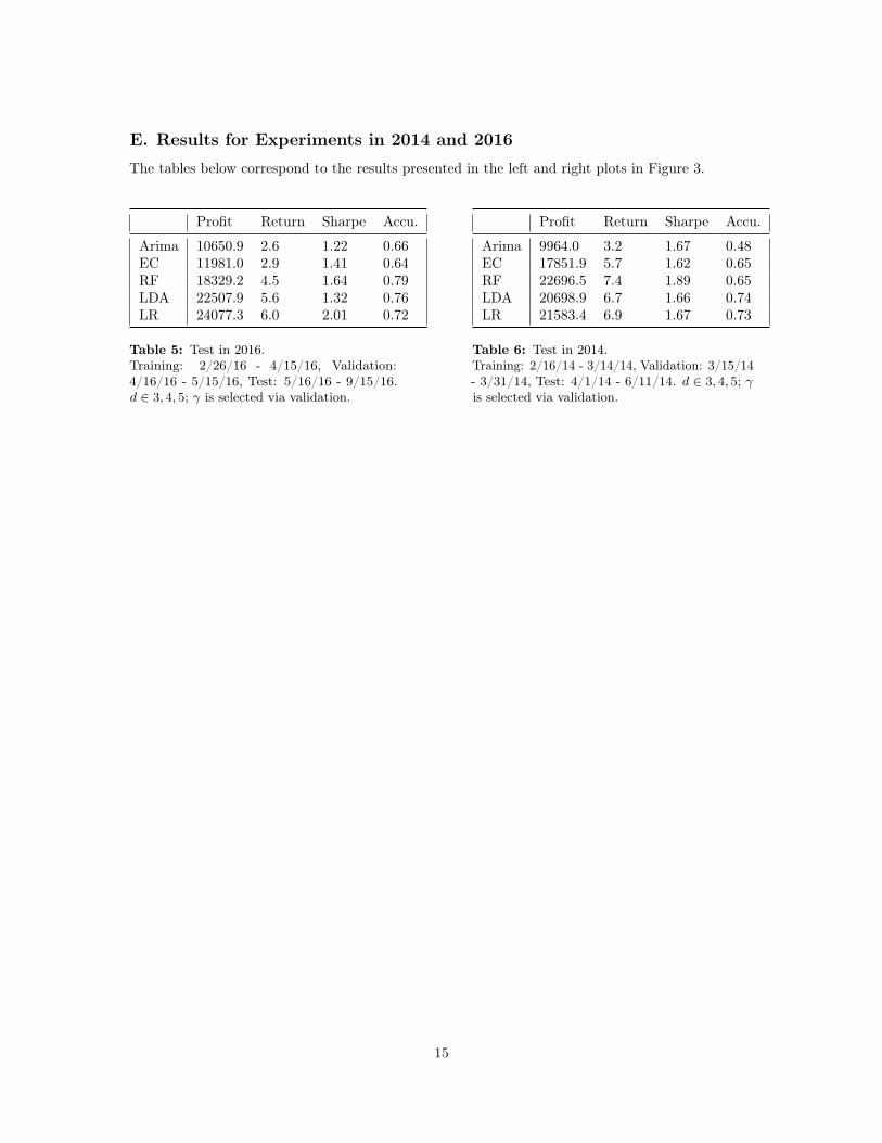
E. Results for Experiments in 2014 and 2016

The tables below correspond to the results presented in the left and right plots in Figure 3.

Profit Return Sharpe Accu.

Arima 10650.9 2.6 1.22 0.66EC 11981.0 2.9 1.41 0.64RF 18329.2 4.5 1.64 0.79LDA 22507.9 5.6 1.32 0.76LR 24077.3 6.0 2.01 0.72

Table 5: Test in 2016.Training: 2/26/16 - 4/15/16, Validation:4/16/16 - 5/15/16, Test: 5/16/16 - 9/15/16.d ∈ 3, 4, 5; γ is selected via validation.

Profit Return Sharpe Accu.

Arima 9964.0 3.2 1.67 0.48EC 17851.9 5.7 1.62 0.65RF 22696.5 7.4 1.89 0.65LDA 20698.9 6.7 1.66 0.74LR 21583.4 6.9 1.67 0.73

Table 6: Test in 2014.Training: 2/16/14 - 3/14/14, Validation: 3/15/14- 3/31/14, Test: 4/1/14 - 6/11/14. d ∈ 3, 4, 5; γis selected via validation.

15