Trade Theory with Numbers:

Quantifying the Consequences of Globalization∗

Arnaud CostinotMIT and NBER

Andrés Rodríguez-ClareUC Berkeley and NBER

March 2013

Abstract

We review a recent body of theoretical work that aims to put numbers on the consequencesof globalization. A unifying theme of our survey is methodological. We rely on gravity modelsand demonstrate how they can be used for counterfactual analysis. We highlight how variouseconomic considerations—market structure, firm-level heterogeneity, multiple sectors, inter-mediate goods, and multiple factors of production—affect the magnitude of the gains fromtrade liberalization. We conclude by discussing a number of outstanding issues in the litera-ture as well as alternative approaches for quantifying the consequences of globalization.

∗This is a draft of a chapter to appear in the Handbook of International Economics, Vol. 4, eds. Gopinath, Helpmanand Rogoff. We thank Rodrigo Rodrigues Adao, Jakub Kominiarczuk, Mu-Jeung Yang, and Yury Yatsynovich forexcellent research assistance. We thank Costas Arkolakis, Edward Balistreri, Dave Donaldson, Jonathan Eaton, KeithHead, Elhanan Helpman, Rusell Hillberry, Pete Klenow, Thierry Mayer, Thomas Rutherford, Robert Stern, Dan Trefler,and Jonathan Vogel for helpful discussions and comments. All errors are our own.

1 Introduction

The theoretical proposition that there are gains from international trade, see Samuelson (1939), isone of the most fundamental result in all of economics. Under perfect competition, opening upto trade acts as an expansion of the production possibility frontier and leads to Pareto superioroutcomes. The objective of this chapter is to survey a recent body of theoretical work that aimsto put numbers on this and other related comparative static exercises, which we will refer to asglobalization.

A unifying theme of our chapter is methodological. Throughout we rely on multi-countrygravity models and demonstrate how they can be used for counterfactual analysis. While so-calledgravity equations have been estimated since the early sixties, see Tinbergen (1962), the widespreaduse of structural gravity models in the field of international trade is a fairly recent phenomenon, asalso discussed by Head and Mayer (2013) in this volume. The previous handbook of internationaleconomics is a case in point. In his opening chapter, Krugman (1995) notes: “the lack of a goodanalysis of multilateral trade in the presence of trade costs is a major gap in trade theory.” Thisview is echoed by Leamer and Levinsohn (1995) who argue that: “The gravity models are strictlydescriptive. They lack a theoretical underpinning so that once the facts are out, it is not clear whatto make of them.” But the times they are a-changin’.

The last ten years have seen an explosion of alternative microtheoretical foundations underly-ing gravity equations; see Eaton and Kortum (2002), Anderson and Van Wincoop (2003), Bernard,Eaton, Jensen, and Kortum (2003), Chaney (2008), and Eaton, Kortum, and Kramarz (2011). Whilenew gravity models encompass a large number of market structures—from perfect competitionto monopolistic competition with firm-level heterogeneity à la Melitz (2003)—and a wide rangeof micro-level predictions, they share the same macro-level predictions regarding the structure ofbilateral trade flows as a function of bilateral costs. It is this basic macro structure and its quanti-tative implications for the consequences of globalization that we will be interested in this chapter.

Recent quantitative trade models based on the gravity equation share the same primary fo-cus as older Computational General Equilibrium (CGE) models; see Baldwin and Venables (1995)for an overview in the previous handbook. The main goal is to use theory in order to derivenumbers—e.g., explore whether particular economic forces appear to be large or small in thedata—rather than pure qualitative insights—e.g., study whether the relationship between two eco-nomic variables is monotone or not in theory. There are, however, important differences betweenold and new quantitative work in international trade that we will try to highlight throughout thischapter. First, new quantitative trade models have more appealing micro-theoretical foundations.One does not need to impose the somewhat ad-hoc assumption that each country is exogenouslyendowed with a distinct good—the so-called “Armington” assumption—to do quantitative workin international trade. Second, recent quantitative papers offer a tighter connection between the-ory and data. Instead of relying on off-the-shelf elasticities, today’s researchers try to use their ownmodel to estimate the key structural parameters necessary for counterfactual analysis. Estimationand computation go hand in hand. Third, new quantitative trade models put more emphasis on

1

transparency and less emphasis on realism. The idea is to construct middle-sized models that arerich enough to speak to first-order features of the data, like the role of country size and geography,yet parsimonious enough so that one can credibly identify its key parameters and understandhow their magnitude affects counterfactual analysis.

Section 2 starts by studying the simplest gravity model possible, the Armington model. Build-ing on Arkolakis, Costinot, and Rodríguez-Clare (2012), we highlight two basic results. First weshow that the changes in welfare associated with globalization, modelled as a change in icebergtrade costs, can be inferred using two variables: (i) changes in the share of expenditure on domes-tic goods; and (ii) the elasticity of bilateral imports with respect to variable trade costs, which werefer to as the trade elasticity. Second we show how changes in bilateral trade flows, in general,and the share of domestic expenditure, in particular, can be computed using only informationabout the trade elasticity and easily accessible macroeconomic data. We refer to this approachpopularized by Dekle, Eaton, and Kortum (2008) as “exact hat algebra.”

Armed with these tools, we illustrate how gravity models can be used to quantify the gainsfrom international trade defined as the (absolute value of) the percentage change in real incomethat would be associated with moving one country from the current, observed trade equilibriumto a counterfactual equilibrium with no trade, i.e. an equilibrium with infinite iceberg trade costs.Since the share of domestic expenditure on domestic goods under autarky is equal to one, thewelfare consequences associated with this counterfactual exercise are easy to compute. Althoughthis is obviously an extreme counterfactual scenario that is (hopefully) not seriously considered bypolicymakers, we view it as a useful benchmark that can shed light on the quantitative importanceof the various channels through which globalization affects the welfare of nations.

Section 3 extends the simple Armington model along several directions. First, we relax theassumption that each country is exogenously endowed with a distinct good and provide alter-native assumptions on technology and market structure under which the counterfactual predic-tions derived in Section 2 remain unchanged. Second, we introduce multiple sectors, interme-diate goods, and multiple factors of production and discuss how these considerations affect theconsequences of globalization. Third, we briefly discuss other extensions including alternativedemand systems—that generate variable markups under monopolistic competition—and multi-national production. Although one can still use macro-level data and a small number of elasticitiesto compute the gains from trade in these richer environments, the results of Section 3 illustrate thatsome realistic departures from the one-sector benchmark, such as the existence of multiple sectorsand tradable intermediate goods tend to increase significantly the magnitude of the gains fromtrade.

Section 4 focuses on evaluating trade policy. Instead of considering the welfare consequencesof a move to autarky, we study counterfactual scenarios in which countries raise their importtariffs, either unilaterally or simultaneously around the world, using the simple Armington model.We then study again how these counterfactual predictions vary across different gravity models.We conclude by discussing how to measure the restrictiveness of trade policy when tariffs are

2

heterogeneous across sectors.Section 5 reviews a number of outstanding issues in the literature. Since the main output of

quantitative trade models are numbers, a fair question is: Are these numbers that we can believein? To shed light on this question, we first discuss the sensitivity of the predictions of gravitymodels to auxiliary assumptions on the nature of trade imbalances and the tradability of capitalgoods. We then turn to the goodness of fit of gravity models in the cross-section and time series.We conclude by discussing how elasticities, i.e., the main inputs of quantitative trade models, arecalibrated.

Sections 6 and 7 discuss other approaches to quantifying the consequences of globalization inthe literature. Section 6 focuses on recent empirical studies that have used micro-level data, eitherat the product or firm-level, to estimate gains from new varieties and productivity gains fromtrade. We discuss how such empirical evidence, i.e., “micro” numbers, relate to the predictionsof gravity models reviewed in this chapter, i.e., “macro” numbers. Section 7 turns to structuralapproaches to quantifying the consequences of globalization that are not based on gravity models.Due to space constraints, we do not review reduced-form evidence on the gains from openness;see e.g. Frankel and Romer (1999), Feyrer (2009a), and Feyrer (2009b). Readers interested in thisimportant topic are referred to the recent survey by Harrison and Rodríguez-Clare (2010).

Section 8 offers some concluding remarks on the current state of the literature and open ques-tions for future research. Additional information about theoretical results and data can be foundin the online Appendix.

2 Getting Started

We start this chapter by describing how to perform counterfactual analysis in the simplest quan-titative trade model possible: the Armington model. A central aspect of this model is the gravityequation; see e.g. Anderson (1979) and Anderson and Van Wincoop (2003). As we will see in thenext section, there exists a variety of microtheoretical foundations that can give rise to a gravityequation, and in turn, a variety of economic environments in which the simple tools introducedin this section can be applied.

2.1 Armington Model

Consider a world economy comprising i = 1, ..., n countries, each endowed with Qi units of adistinct good i = 1, ..., n.

Preferences. Each country is populated by a representative agent whose preferences are repre-sented by a Constant Elasticity of Substitution (CES) utility function:

Cj =(

∑ni=1 ψ

(1−σ)/σij C(σ−1)/σ

ij

)σ/(σ−1), (1)

where Cij is the demand for good i in country j; ψij > 0 is an exogenous preference parameter;

3

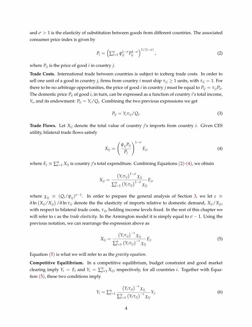
and σ > 1 is the elasticity of substitution between goods from different countries. The associatedconsumer price index is given by

Pj =(

∑ni=1 ψ1−σ

ij P1−σij

)1/(1−σ), (2)

where Pij is the price of good i in country j.

Trade Costs. International trade between countries is subject to iceberg trade costs. In order tosell one unit of a good in country j, firms from country i must ship τij ≥ 1 units, with τii = 1. Forthere to be no arbitrage opportunities, the price of good i in country j must be equal to Pij = τijPii.The domestic price Pii of good i, in turn, can be expressed as a function of country i’s total income,Yi, and its endowment: Pii = Yi/Qi. Combining the two previous expressions we get

Pij = Yiτij/Qi. (3)

Trade Flows. Let Xij denote the total value of country j’s imports from country i. Given CESutility, bilateral trade flows satisfy

Xij =

(ψijPij

Pj

)1−σ

Ej, (4)

where Ej ≡ ∑ni=1 Xij is country j’s total expenditure. Combining Equations (2)-(4), we obtain

Xij =

(Yiτij

)1−σχij

∑nl=1(Ylτl j

)1−σχl j

Ej,

where χij ≡ (Qi/ψij)σ−1. In order to prepare the general analysis of Section 3, we let ε ≡

∂ ln(Xij/Xjj

)/∂ ln τij denote the the elasticity of imports relative to domestic demand, Xij/Xjj,

with respect to bilateral trade costs, τij, holding income levels fixed. In the rest of this chapter wewill refer to ε as the trade elasticity. In the Armington model it is simply equal to σ− 1. Using theprevious notation, we can rearrange the expression above as

Xij =

(Yiτij

)−εχij

∑nl=1(Ylτl j

)−εχl j

Ej. (5)

Equation (5) is what we will refer to as the gravity equation.

Competitive Equilibrium. In a competitive equilibrium, budget constraint and good marketclearing imply Yi = Ei and Yi = ∑n

j=1 Xij, respectively, for all countries i. Together with Equa-tion (5), these two conditions imply

Yi = ∑nj=1

(Yiτij

)−εχij

∑nl=1(Ylτl j

)−εχl j

Yj. (6)

4

This provides a system of n equations with n unknowns, Y≡Yi. By Walras’ Law, one of theseequations is redundant. Thus income levels are only determined up to a constant. Once incomelevels are known, expenditure levels, E≡Ei, can be computed using budget constraint andbilateral trade flows, X≡

Xij

, can be computed using the gravity equation. This concludes thedescription of the Armington model.

2.2 Counterfactual Analysis

We now illustrate how the gravity equation can be used to quantify the welfare consequencesof globalization. For simplicity, we focus on a shock to trade costs from τ≡

τij

to τ′≡

τ′ij

.

The same analysis generalizes in a straightforward manner to preference and endowment shocks.To quantify the welfare consequences of a trade shock in a given country j, we proceed in twosteps. First, we show how changes in real consumption, Cj≡Ej/Pj, can be inferred from changesin macro variables, X and Y. Second, we show how to compute changes in macro variables.

Welfare. In this chapter, whenever we refer to welfare changes in country j, we refer to percentagechanges in real consumption. Such changes correspond to the equivalent variation associatedwith a foreign shock (expressed as a share of expenditure before the shock). Namely, percentagechanges in real consumption measures the percentage change in income that the representativeagent would be willing to accept in lieu of the shock to happen.

The first result that we establish is that changes in real consumption can be inferred using onlytwo statistics: (i) observed changes in the share of expenditure on domestic goods, λjj ≡ Xjj/Ej;and (ii) the trade elasticity in the gravity equation, ε.

Let us start by considering an infinitesimal change in trade costs from τ to τ + dτ. By Shep-hard’s Lemma, we know that

d ln Pj = ∑ni=1 λijd ln Pij,

where λij≡Xij/Ej denotes the share of expenditure on goods from country i in country j. Sinceconsumption is chosen to minimize expenditure, changes in consumption levels, Cij, only havesecond-order effects on the consumer price index in country j. Under the assumption of CESutility, changes in the consumer price index in country j can be rearranged further into changesinto domestic and import prices

d ln Pj = λjjd ln Pjj +(1− λjj

)d ln PM

j ,

where PMj ≡

[∑i 6=j P1−σ

ij

]1/(1−σ)is the component of the price index associated with imports. By

differentiating Equation (4), one can also show that

d ln(1− λjj

)− d ln λjj = (1− σ)

(d ln PM

j − d ln Pjj

).

5

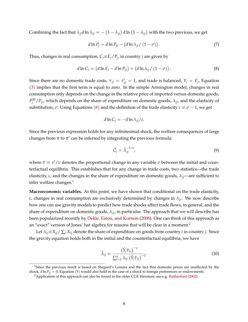
Combining the fact that λjjd ln λjj = −(1− λjj

)d ln

(1− λjj

)with the two previous, we get

d ln Pj = d ln Pjj −(d ln λjj/ (1− σ)

). (7)

Thus, changes in real consumption, Cj≡Ej/Pj, in country j are given by

d ln Cj =(d ln Ej − d ln Pjj

)+(d ln λjj/ (1− σ)

). (8)

Since there are no domestic trade costs, τ jj = τ′jj = 1, and trade is balanced, Yj = Ej, Equation(3) implies that the first term is equal to zero. In the simple Armington model, changes in realconsumption only depends on the change in the relative price of imported versus domestic goods,PM

j /Pjj, which depends on the share of expenditure on domestic goods, λjj, and the elasticity ofsubstitution, σ. Using Equations (8) and the definition of the trade elasticity ε ≡ σ− 1, we get

d ln Cj = −d ln λjj/ε.

Since the previous expression holds for any infinitesimal shock, the welfare consequences of largechanges from τ to τ′ can be inferred by integrating the previous formula:

Cj = λ−1/εjj , (9)

where v ≡ v′/v denotes the proportional change in any variable v between the initial and coun-terfactual equilibria. This establishes that for any change in trade costs, two statistics—the tradeelasticity, ε, and the changes in the share of expenditure on domestic goods, λjj—are sufficient toinfer welfare changes.1

Macroeconomic variables. At this point, we have shown that conditional on the trade elasticity,ε, changes in real consumption are exclusively determined by changes in λjj. We now describehow one can use gravity models to predict how trade shocks affect trade flows, in general, and theshare of expenditure on domestic goods, λjj, in particular. The approach that we will describe hasbeen popularized recently by Dekle, Eaton, and Kortum (2008). One can think of this approach asan “exact” version of Jones’ hat algebra for reasons that will be clear in a moment.2

Let λij≡Xij/ ∑l Xl j denote the share of expenditure on goods from country i in country j. Sincethe gravity equation holds both in the initial and the counterfactual equilibria, we have

λij =

(Yiτij

)−ε

∑nl=1 λl j

(Yl τl j

)−ε . (10)

1Since the previous result is based on Shepard’s Lemma and the fact that domestic prices are unaffected by theshock, d ln Pjj = 0, Equation (9) would also hold in the case of a shock to foreign preferences or endowments.

2Application of this approach can also be found in the older CGE literature; see e.g. Rutherford (2002).

6

In the counterfactual equilibrium, Equation (6) further implies

Y′j = ∑ni=1 λ′jiY

′i .

Combining the two previous expressions, we then get

YjYj = ∑ni=1

λji(Yjτ ji

)−εYiYi

∑nl=1 λli

(Yl τli

)−ε . (11)

Although trade costs, endowments, and preference shifters affect bilateral trade flows, as capturedby τij and χij in equation (5), Equation (11) shows that we can compute counterfactual changes inincome, Y≡

Yi

, as the solution of a system of non-linear equations without having to estimateany of these parameters. All we need to determine changes in income levels (up to normalization)are the initial expenditure shares, λij, the initial income levels, Yi, and the trade elasticity, ε. Givenchanges in income levels, changes in the shares of expenditure on goods from different countries,λij, and changes in real consumption, Cj, can then be computed using Equations (9) and (10).

2.3 Trade Theory with Numbers: A Preview

In order to illustrate the usefulness of the simple Armington model, we focus on a very particular,but important counterfactual exercise: moving to autarky. Formally, we assume that variable tradecosts in the new equilibrium are such that τ′ij = +∞ for any pair of countries i 6= j. All otherstructural parameters are the same as in the initial equilibrium. For this particular shock, we donot need to solve any non-linear system of equations to do counterfactual analysis. Since the shareof expenditure on domestic goods must be equal to 1 in the counterfactual equilibrium, λ′jj = 1,we immediately know that λjj = 1/λjj.

Throughout this chapter we define the gains from international trade in country j, Gj, as theabsolute value of the percentage change in real income that would be associated with moving toautarky in country j. Using Equation (9) and the fact that λjj = 1/λjj, we get

Gj = 1− λ1/εjj . (12)

In order to compute Gj we need measures of the trade elasticity, ε, and the share of expenditureon domestic goods, λjj. There are many econometric issues associated with estimating ε; see e.g.Hummels and Hillberry (2012). A simple way to estimate the trade elasticity ε is to take the log ofthe gravity equation (5) and run a cross-sectional regression of the following form

ln Xij = δXi + δM

j − ε ln τij + δij, (13)

where the first term δXi ≡ ln χi − ε ln Yi is treated as an exporter fixed-effect; the second term

δMj ≡ ln Yj − ln

[∑n

l=1 χl(Ylτl j

)−ε]

is treated as an importer fixed-effect; and the third term δij is

7

treated as measurement error in trade flows that is orthogonal to ln τij. At this point we set ε = 5,which is a typical value used in the literature; see e.g. Anderson and Van Wincoop (2004) andHead and Mayer (2013). We will come back to the sensitivity of our quantitative results to valuesof the trade elasticity in Section 5.

In order to measure λjj in the data, recall that λjj ≡ Xjj/Ej = 1− ∑i 6=j Xij/ ∑ni=1 Xij. We can

measure ∑i 6=j Xij as total imports by country j, whereas ∑i Xij is total expenditure by country j.In this exercise as well as all subsequent exercises, we use data from the World Input-OutputDatabase (WIOD) in 2008. The database covers 27 EU countries and 13 other major countries; seeTimmer (2012).3 The first column of Table 1 reports the gains from trade Gj for these countriesusing Equation (12). According to the simple Armington model, we see that gains from tradeare below 2% for three countries: Brazil (1.5%), Japan (1.7%), and the United States (1.8%). Notsurprisingly, gains from trade tend to be larger for smaller countries. The largest predicted gainsare for Slovakia (7.6%), Ireland (8.0%) and Hungary (8.1%). Given the strong assumptions thathave been imposed in Section 2.1, these numbers, of course, should be taken with more than agrain of salt. We now discuss how richer and more realistic models would affect the magnitude ofthe gains from trade.

3 Beyond Armington

The Armington model is very tractable, which has made it the go-to trade model for quantitativework in policy institutions for more than forty years. This is also a very stylized model, which haslead to quite a bit of skepticism about the robustness of its counterfactual predictions in academiccircles for about as many years. Fortunately, one can maintain the tractability of the Armingtonmodel, without maintaining the somewhat ad-hoc assumption that each country is exogenouslyendowed with a distinct good. As discussed below, the gravity equation (5), which is the basis forcounterfactual analysis in the Armington model, can be shown to hold under various assumptionsabout technology and market structure. While each gravity model remains special, in the sensethat strong functional form assumptions are required for a gravity equation to hold, the ability ofthese new models to match a large number of micro-level facts, together with the elegance of theirmicrotheoretical foundations, has lead to an explosion of quantitative work in international tradeover the last ten years.

In this section we explore how various features of more complex gravity models—marketstructure, firm-level heterogeneity, multiple sectors, intermediate goods, and multiple factors ofproduction—affect the gains from trade as defined in Section 2.3. Throughout our analysis we

3The mapping between the simple Armington model presented here and the data is not trivial for two reasons: (i)it assumes the share of expenditures on intermediate goods is zero and (ii) it assumes that trade is balanced. Thisimplies that GDP is equal to gross output and that total expenditure is equal to GDP. Neither is true in the data. Wewill deal with intermediate goods and trade imbalances explicitly in Sections 3.4 and 5.1, respectively. Here, as well asin Section 3, we derive and apply our formulas for gains from trade ignoring trade imbalances. If moving to autarkyalso implies the closing of trade imbalances, our formulas capture the change in real income rather than the change inreal expenditure. See online Appendix for details.

8

calibrate different models to match the same moments in the macro-data, including bilateral tradeflows and trade elasticities. Thus different models may lead to different predictions about themagnitude of the gains from trade because they predict different counterfactual autarky equilib-ria, not because they predict different trade volumes in the initial equilibrium. In short, tradevolumes are taken as data that discipline the behavior of all models, irrespectively of what theirparticular micro-theoretical foundations may be.4

As explained in the Introduction, although a move to autarky is an extreme comparative staticsexercise, it should be viewed as a useful benchmark to study the importance, in a well-definedwelfare sense, of various economic channels discussed in the literature. We leave the evaluationof trade policy to Section 4 in which we show how to use the exact hat algebra to conduct richercomparative static exercises.

3.1 Many Models, One Equation

The gravity equation (5) has been shown to hold under perfect competition, as in Eaton and Ko-rtum (2002); under Bertrand competition, as in Bernard, Eaton, Jensen, and Kortum (2003); undermonopolistic competition with homogeneous firms, as in Krugman (1980); and under monopo-listic competition with firm-level heterogeneity, as in Chaney (2008), Arkolakis (2010), Arkolakis,Demidova, Klenow, and Rodríguez-Clare (2008), and Eaton, Kortum, and Kramarz (2011). Ourgoal in this subsection is not to describe each of these models in detail, but rather highlight thecommon features that will lead to a gravity equation as well as the key differences that may affectthe magnitude of the gains from trade. Detailed discussions of the microfoundations and func-tional form assumptions leading to gravity equations can be found in Anderson (2010), Arkolakis,Costinot, and Rodríguez-Clare (2012), Head and Mayer (2013), as well as in our online Appendix.

Like the simple Armington model, the alternative gravity models mentioned above assumethe existence of a representative agent with CES utility in each country as well as balanced trade,Ei = Yi.5 The representative agent, however, now has preferences over a continuum of goods orvarieties ω ∈ Ω:

Cj =

(∫ω∈Ω

cj(ω)(σ−1)/σdω

)σ/(σ−1)

,

with σ > 1. In equilibrium, each good ω is only imported from one country so that Equation (1)still holds with the aggregate consumption of goods from country i in country j being given byCij =

∫ω∈Ωij

cj(ω)(σ−1)/σdω, where Ωij ⊂ Ω denotes the set of goods that country j buys from

country i, and ψij = 1 for all country pairs due to the symmetry across varieties. For the samereason, Equation (2) holds as well with the aggregate price of goods from country i in country j

being given by Pij =(∫

ω∈Ωijpj(ω)

1−σdω)1/(1−σ)

and ψij = 1 for all i and j.

4In order to match the same cross-section of trade flows, different gravity models may implictly rely on differentvalues of bilateral trade costs as well as other structural parameters.

5In recent work, Arkolakis, Costinot, Donaldson, and Rodriguez-Clare (2012) have developed a gravity model with-out CES utility. We discuss the implications of such a model in Section 3.6.

9

A key difference between the simple Armington model and the alternative gravity modelsmentioned above is that, due to different assumptions on technology and market structure, Ωij isno longer exogenously given. In these richer models, firms from country i may now decide to stopproducing and selling a subset of goods in country j if it is not profitable for them to do so. Hencechanges in prices, Pij, may reflect both: (i) changes at the intensive margin, i.e., changes in theprice of goods imported in country j, pj(ω), and (ii) changes at the extensive margin, i.e., changesin the set of good imported in country j, Ωij, due either to the selection of a different subset offirms from i in j or the entry of a different set of firms in i. Mathematically, these new economicconsiderations lead to the following generalization of Equation (3):

Pij = τijcpi︸︷︷︸

Intensive Margin

×

(Ej

cxij

) δ1−σ τijc

pi

Pj

η

︸ ︷︷ ︸Extensive Margin: Selection

×(

Ri

cei

) δ1−σ

︸ ︷︷ ︸Extensive Margin: Entry

× ξ ij, (14)

where cpi , ce

i , and cxij are endogenous variables that capture how input prices affect variable costs

of production, fixed entry costs, and fixed exporting costs, respectively; Ej ≡ ∑ni=1 Xij still denotes

total expenditure in country j; Ri ≡ ∑j Xij denotes total sales or revenues for producers; and ξ ij >

0 is a function of structural parameters distinct from variable trade costs, τij, such as endowmentsor fixed exporting costs. The last two parameters, δ and η, will play a central role in our analysis.The parameter δ is a dummy variable that characterizes the market structure: it is equal to oneunder monopolistic competition with free entry and zero under perfect or Bertrand competition.6

The parameter η ≥ 0 is related to the extent of heterogeneity across varieties as we discuss moreformally below.

In the rest of this chapter we will use Equation (14) to organize the literature and explainhow different assumptions about technology and market structure—namely, different assump-tions about cp

i , cei , cx

ij, δ, and η—may lead to different macro-level predictions without getting lostinto the algebra through which Equation (14) comes about. At this point, it is therefore importantto clarify how each term in Equation (14) relates to previous work in the literature.

The first term, τijcpi , captures price changes at the intensive margin. This is the only active

margin in the Armington model. In that model, cpi = Yi, δ = 0, and η = 0; see Equation (3).

This intensive margin will remain active in all models that we study. In most of these models, cpi

will also remain equal to total income Yi in country i. This is the case, for instance, if labor is theonly factor of production. In this situation, production costs are proportional to wages, which areproportional to countries’ total income.

The second term,((

Ej/cxij

) δ1−σ

τijcpi /Pj

)η

, captures changes at the extensive margin due to

selection effects. If η = 0, then this term is equal to one and there are no selection effects. Thisoccurs in models of monopolistic competition without firm-level heterogeneity and fixed export-

6For expositional purposes, we often abuse terminology in this chapter and simply refer to the case δ = 1 and δ = 0as “monopolistic competition” and “perfect competition,” respectively.

10

ing costs, like Krugman (1980), in which all firms always export. The case η > 0 captures insteadsituations in which a subset of firms from country i may start or stop exporting when market con-ditions change in country j. Specifically, in models of perfect competition, like Eaton and Kortum(2002), Bertrand competition, like Bernard, Eaton, Jensen, and Kortum (2003), or monopolisticcompetition à la Melitz (2003), like Chaney (2008), Arkolakis, Demidova, Klenow, and Rodríguez-Clare (2008), Arkolakis (2010), and Eaton, Kortum, and Kramarz (2011), if firms from country i areless competitive relative to other firms serving market j, i.e., τijc

pi /Pj is high, then less firms from

country i will serve this market, which will lead to a decrease in the number of varieties from iavailable in j and an increase in Pij. In the previous models, the magnitude of selection effectsis formally determined by η ≡

(θ

σ−1

) (1+ 1−σ

θ

), where θ > σ − 1 is the shape parameter of the

distribution of productivity draws across varieties. Under perfect and Bertrand competition, thisdistribution is Fréchet. Under monopolistic competition, it is Pareto. In both cases, θ measures theelasticity of the mass of goods produced domestically with respect to their relative cost; 1/ (1− σ)

measures the elasticity of the price index with respect to new goods; and(1+ 1−σ

θ

)corrects for

the fact that the marginal variety has a higher price than the average variety. In models of monop-olistic competition with firm-level heterogeneity à la Melitz (2003) (δ = 1,η > 0), selection alsodepends on the size of market j relative to the fixed costs of exporting from i to j, which is reflected

in(

Ej/cxij

) δ1−σ

. The nature of cxij depends on where fixed exporting costs are paid. If they are paid

in the exporting country, then cxij is proportional to total income, Yi, in country i. If they are paid

in the importing country, then cxij is proportional to total income, Yj, in country j.

The third term,(

Ri/cei) δ

1−σ , captures changes at the extensive margin due to entry effects. Thislast channel is specific to models with monopolistic competition and free entry (δ = 1), whetheror not they feature firm-level heterogeneity à la Melitz (2003).7 In such environments, countriesin which entry is more profitable, i.e., Ri/ce

i is high, export more varieties to all countries, whichdecreases the price index with an elasticity 1/ (σ− 1). If entry costs are paid in terms of labor, asin Krugman (1980) or Melitz (2003), ce

i is simply proportional to total income Yi in country i.To sum up, starting from Equation (14), we can turn off and on the selection effects associated

with heterogeneity across varieties by setting η to 0 or not. Similarly, we can turn off and onthe scale effects associated with monopolistic competition and free entry by setting δ to 0 or 1.In the next subsections, we study how much these considerations—as well as the introductionof multiple sectors, tradable intermediate goods, and multiple factors of production—affect theoverall magnitude of the gains from trade.

7Without free entry,(

Ri/cei) δ

1−σ would be absent from Equation (14) and one would need, in general, to take intoaccount the effect of trade on profits; see e.g. Ossa (2011a). In the one-sector case reviewed in the next subsection,this distinction turns out to be irrelevant, as shown in Arkolakis, Costinot, and Rodríguez-Clare (2012). With multiplesectors, however, free entry leads to home market effects, with implications for the magnitude of the gains from trade.

11

3.2 One Sector

It is standard to interpret models with CES utility, such as those presented in Section 3.1, as one-sector models with a continuum of varieties; see e.g. Helpman and Krugman (1985). Here wefocus on such models since they are the closest to the Armington model described in Section 2.1.Later we will consider multi-sector extensions of these models as well as incorporate tradableintermediate goods and multiple factors of production.

In line with the existing literature, we assume that, in addition to Equation (14), the two fol-lowing conditions hold: (i) cp

i = cxii = ce

i = Yi, which reflects the fact that all factors of productionare used in the same proportions to produce, export, and develop all varieties; and (ii) Ri = Yi,which reflects the fact that trade in goods is balanced.8 Under these two conditions, Equation (14)simplifies into

Pij = τijYi

(Ej

cxij

) δ1−σ τijYi

Pj

η

ξ ij, (15)

Note that Ri = Yi = cei implies that, like in the Armington model, there are no entry effects

associated with changes in trade costs, even under monopolistic competition. Since Equation (1)still holds, bilateral trade flows between country i and country j are still given by Equation (4).Combining this observation with Equation (15), the gravity equation generalizes to

Xij =

(Yiτij

)−ε(

cxij

)−δηχij

∑nl=1(Ylτl j

)−ε(

cxlj

)−δηχl j

Ej. (16)

Compared to the Armington model, here ε = (1+ η) (σ− 1) and χij ≡ ξ1−σij . Thus if there are

selection effects, i.e., if η 6= 0, the structural interpretation of the trade elasticity is no longerthe same as in the Armington model. This reflects the fact that changes in variable trade costsnow affect both the price of existing varieties (intensive margin) and the set of varieties sold fromcountry i to country j (extensive margin). Nevertheless, we can still take the logs of both sidesof Equation (4) and estimate the trade elasticity ε as we did in Section 2.3. In other words, themapping between bilateral trade data, X, and the trade elasticity, ε, remains unchanged.9 Finally,

we see that changes in the magnitude of fixed exporting costs, as captured by(

cxij

)−δη, now affect

bilateral trade flows under monopolistic competition with firm-level heterogeneity à la Melitz(2003), i.e., if δ = 1, η > 0.10 This extra term—which depends on whether fixed exporting costs

8Since some of the models that we consider involve fixed exporting costs paid in the importing country, i.e. trade inexporting services, the assumption that overall trade is balanced, Ei = Yi, is different from the assumption that tradein goods is balanced, Ri = Yi. The latter condition corresponds to the macro-level restriction R1 in Arkolakis, Costinot,and Rodríguez-Clare (2012).

9This assumes that measures of trade costs are invariant across models. This is a reasonable assumption in the caseof import tariffs, but not in the case of price gaps; see Simonovska and Waugh (2012). We come back to the specificissues associated with import tariffs in Section 4.

10Equation (16) is a special case of the macro-level restriction R3 in Arkolakis, Costinot, and Rodríguez-Clare (2012).Compared to Arkolakis, Costinot, and Rodríguez-Clare (2012), we no longer need to impose explictly that profits are

12

are paid in the importing country, the exporting country, or both—opens up the possibility ofdifferent predictions across gravity models, as we explain below.

Like in Section 2.2, consider a change in variable trade costs from τ ≡

τij

to τ′ ≡

τ′ij

,

though the same analysis easily extends to shocks to foreign endowments or technology, i.e.,changes in χ≡

χij

. Given CES utility, Equation (8) still holds. The key difference compared

to our previous analysis is that d ln Ej − d ln Pjj is no longer equal to zero. Because of selectioneffects, a change in variable trade costs may lead to a change in the set of goods produced do-mestically, Ωjj, and so to a change in the aggregate price index associated with these goods, Pjj,relative to total expenditure in country j. Specifically, since Ej = Yj and cx

jj = Yj, Equation (15)implies

d ln Pjj = (1+ η) d ln Yj − ηd ln Pj.

Using the previous expression with Equation (7), which still holds because of CES utility, and thetrade balance condition, Ej = Yj, we then get

d ln Ej − d ln Pjj = − (η/ (η + 1))×(d ln λjj/ (1− σ)

). (17)

In models featuring selection effects (η > 0), a positive terms-of-trade shock, d ln λjj/ (1− σ) > 0,is accompanied by a negative shock to real consumption of domestic goods, d ln Ej − d ln Pjj < 0.Intuitively, a positive terms-of-trade shock tends to decrease the profitability of domestic firms onthe domestic market, which leads to a decrease in the number of goods produced domestically,and, given the love of varieties embedded in CES utility functions, an increase in the aggregateprice index associated with these goods.

Together with ε = (1+ η) (σ− 1), Equations (8) and (17) imply d ln Cj = −d ln λjj/ε. Like inthe Armington model, the previous expression can be integrated to get Equation (9).11 Thus, asestablished in Arkolakis, Costinot, and Rodríguez-Clare (2012), changes in the share of expendi-ture on domestic goods, λjj, and the trade elasticity, ε, remain two sufficient statistics for welfareanalysis. In particular, gains from trade remain given by Equation (12). In short, conditional onobserved trade flows and the trade elasticity, selection and scale effects have no impact on theoverall magnitude of the gains from trade.

The fact that λjj remains the only macro variable that matters for welfare is intuitive enough:it measures the magnitude of the terms-of-trade effect and changes in real output themselvesare function of changes in the overall price index, which also depends on the magnitude of theterms-of-trade effect. The fact that the only structural parameter that matters can be recovered asthe trade elasticity ε from a gravity equation, by contrast, heavily relies on the fact that selectioneffects, as captured by η, are identical across countries. It is this assumption that simultaneouslygenerates a gravity equation and guarantees that the trade elasticity in that equation is the relevant

proportional to revenues. This restriction is implicit in Equation (15).11A more direct, though perhaps less illuminating way of establishing Equation (9) consists in computing Pjj from

Equation (15) and substituting for it in λjj =(

Pjj/Pj

)1−σ.

13

elasticity for welfare analysis. It is worth noting that this result does not rely on the fact that newvarieties have zero welfare effects. In the models with monopolistic competition considered here,a shock to trade costs, foreign endowments, or foreign technology, may very well increase welfarethrough its effects at the extensive margin. The point rather is that these effects, no matter howlarge they are, can always be inferred from changes in aggregate trade flows.

The previous equivalence only establishes that conditional on a change in λjj and ε, alternativegravity models must predict the same welfare change as the Armington model, but, in principle,they may predict different changes in the share of domestic expenditure for a given trade shock.Under the additional assumption that fixed exporting costs (if any) are paid in the destinationcountry—cx

ij = cxj , as in Eaton, Kortum, and Kramarz (2011)—one can show a stronger equivalence

result. In that case, cxij drops out of Equation (16). Thus the counterfactual changes in trade

flows and income levels associated with changes in variable trade costs can still be computedusing the exact hat algebra of Section 2.2, i.e. Equations (10) and (11). Given observable macrovariables in the initial equilibrium, X and Y , and a value of the trade elasticity, ε, this impliesthat counterfactual predictions for macro variables and welfare are exactly the same as in theArmington model.12 This stronger equivalence result, however, is very sensitive to the assumptionthat fixed exporting costs are paid in the importing country. If fixed exporting costs are partly paidin the origin country, then one-sector gravity models with monopolistic competition and firm-level heterogeneity à la Melitz (2003) generally predict different changes in relative factor prices,i.e., relative wages if labor is the only factor of production. This leads to different changes in theshare of expenditure on domestic goods and, in turn, different welfare changes for a given changein trade costs (moving to autarky being a notable exception).13

3.3 Multiple Sectors

Gravity models can be extended to multiple sectors, s = 1, ..., S, by assuming a two-tier utilityfunction in which the upper-level is Cobb-Douglas and the lower-level is CES; see e.g. Andersonand Yotov (2010), Donaldson (2008), Caliendo and Parro (2010), Costinot, Donaldson, and Ko-munjer (2010), Hsieh and Ossa (2011), Levchenko and Zhang (2011), Ossa (2012), Shikher (forth-cominga), and Shikher (forthcomingb). Formally let us assume that the representative agent in

12In this special case, one can show that the welfare impact of changes in the number of domestic varieties (if any)exactly compensates the welfare impact of changes in the number of foreign varieties (if any), as emphasized in Feenstra(2010). In general, i.e., if fixed costs are partly paid in the origin country, these exact offsetting effects no longer hold,though the welfare change associated with a shock to variable trade costs remains given by Equation (9), as discussedabove. Similarly, in the case of shocks to foreign endowments or technology, these exact offsetting effects no longerhold, though welfare changes remain given by Equation (9), as shown in Arkolakis, Costinot, and Rodríguez-Clare(2012). In short, the main equivalence result in Arkolakis, Costinot, and Rodríguez-Clare (2012) does not hinge on theseexact offsetting effects.

13For finite changes in trade costs, different counterfactual predictions do not arise from selection effects per se, butrather from the fact that fixed exporting costs, if paid at least partly in the origin country, can affect relative demandfor factors of production in different countries and so relative factor prices. To see this, note that in a symmetric worldeconomy in which relative factor prices are constant, cx

ij would be constant across countries as well. Thus, in spite ofselection effects, cx

ij would again drop out of Equation (16), leading to the same counterfactual predictions as in theArmington model.

14

each country aims to maximize

Cj = ∏Ss=1 C

βj,sj,s , (18)

where βj,s ≥ 0 are exogenous preference parameters satisfying ∑Ss=1 βj,s = 1 and Cj,s is total con-

sumption of the composite good s in country j,

Cj,s =

(∫ω∈Ω

cj,s(ω)(σs−1)/σs dω

)σs/(σs−1)

, (19)

where σs > 1 is the elasticity of substitution between different varieties, which is allowed tovary across sectors. In multi-sector gravity models, each variety remains sourced from only one

country so that a sector level version of (1) still holds, Cj,s =(

∑ni=1 C(σs−1)/σs

ij,s

)σs/(σs−1), with

Cij,s =∫

ω∈Ωij,scj,s(ω)

(σs−1)/σs dω. The associated consumer price index is Pj = ∏Ss=1 P

βj,sj,s , with

sector-specific price indices given by a sector level version of (2), Pj,s =(

∑ni=1 P1−σs

ij,s

)1/(1−σs), with

Pij,s =(∫

ω∈Ωij,spj,s(ω)

(1−σs)dω)1/(1−σs)

.In line with the literature, we assume that our reduced-form assumption on price indices,

Equation (14), now holds sector-by-sector; that factors of production are used in the same wayacross all activities in all sectors, so that cp

i,s = cmii,s = ce

i,s = Yi; and that trade in goods is balanced,Ri = Yi.14 Combining these assumptions, we get

Pij,s = τij,sYi

(ej,sEj

cxij,s

) δs1−σs τij,sYi

Pj,s

ηs

rδs

1−σsi,s ξ ij,s. (20)

where ej,s ≡ Ej,s/Ej denotes the share of total expenditure in country j allocated to sector s andri,s = Ri,s/Ri denote the share of total revenues in country i generated from sector s. All othervariables have the same interpretation as in Section 3.1, except that they are now free to vary acrosssectors. Compared to Equation (15), Equation (20) allows for scale effects in monopolistically

competitive sectors both through selection,(

ej,sEj/cxij,s

) δs1−σs , and entry, r

δs1−σsi,s . In the one-sector

case, the latter effect is necessarily absent because ri,s = 1. Here an expansion of production in amonopolistically competitive sector, i.e. a higher value of ri,s, leads to entry and gains from newvarieties, i.e. a lower value of Pij,s, with the standard “love of variety” elasticity of 1/ (σs − 1).15

We now focus on the gains from international trade, as defined in Section 2.3, and discuss howthey are affected by the introduction of multiple sectors under the assumption that Equation (20)holds. Bilateral trade flows at the sector-level satisfy Xij,s =

(Pij,s/Pj,s

)1−σs ej,sEj. Together with

14The assumption, Ri = Yi, is stronger than in the one-sector case. In Section 3.2, it holds in models with monopolisticcompetition and firm-level heterogeneity independently of where fixed exporting costs are paid, as long as productivitydistributions are Pareto. In a multi-sector environment, this may no longer be true even under Pareto if fixed exportingcosts are partly paid in the importing country and sectors differ in the share of revenues associated with fixed exportingcosts. Such considerations lead to a slight change in the present analysis, which we come back to below.

15Similar scale effects can be introduced in the one sector case by allowing factor supply to be elastic; see Balistreri,Hillberry, and Rutherford (2009). The magnitude of such effects then crucially depends on the elasticity of factor supply.

15

Equation (20), this implies the sector-level gravity equation:

Xij,s =

(τij,sYi

)−εs(

cxij

)−δsηsrδs

i,sχij,s

∑l(τl j,sYl

)−εs(

cxlj,s

)−δsηsrδs

l,sχl j,s

ej,sEj, (21)

where εs = (1+ ηs) (σs − 1) and χij,s ≡ ξ1−σsij,s . As in Section 3.1, one can combine Equation (20),

Equation (21), and the fact that λjj,s =(

Pjj,s/Pj,s)1−σs to show that changes in real consumption

associated with a trade shock are now given by:

Cj = ∏Ss=1

(λjj,s

(eηs

j,srj,s

)−δs)−βj,s/εs

. (22)

Under Cobb-Douglas preferences, we know that ej,s = e′j,s = βj,s. Thus the previous expression

can be simplified further into Cj = ∏Ss=1

(λjj,sr

−δsj,s

)−βj,s/εs.16 To compute the gains from trade, we

only need to solve for rj,s when the counterfactual entails autarky. Since r′j,s = e′j,s under autarkyand ej,s = e′j,s = βj,s, we must have rj,s = ej,s/rj,s. Using the fact that λjj,s = 1/λjj,s for all s, wethen get

Gj = 1−∏Ss=1

(λjj,s

(ej,s

rj,s

)δs)βj,s/εs

. (23)

Since δs appears in Equation (23), gains from trade predicted by multi-sector gravity models withmonopolistic competition differ from those predicted by models with perfect competition becauseof scale effects, as discussed in Arkolakis, Costinot, and Rodríguez-Clare (2012). In contrast, se-lection effects still have no impact on the overall magnitude of the gains from trade. Since ηs doesnot appear in Equation (23), conditional on observed trade flows and the trade elasticity, the gainsfrom trade predicted by monopolistically competitive gravity models with and without firm-levelheterogeneity are the same, even with multiple sectors.

To compute the gains from trade using Equation (23), we need measures of λjj,s, ej,s, βj,s andrj,s as well as sector-level trade elasticities εs for s = 1, ..., S. To compute λjj,s, ej,s, βj,s and rj,s, weuse data on 31 sectors from the WIOD in 2008, as explained in the Appendix.17 Trade elasticitiesfor agriculture and manufacturing sectors are from Caliendo and Parro (2010) while the tradeelasticity for service sectors is simply held equal to the aggregate elasticity used in Section 2.3, 5.18

For the purposes of this chapter, the main advantage of the estimation procedure in Caliendo andParro (2010) is that it is consistent with all quantitative trade models satisfying the sector-level

16Without balanced trade in goods, Rj 6= Yj, this would generalize to Cj = ∏Ss=1

(λjj,s

(rj,sRj/Yj

)−δs)−βj,s/εs

.17In theory, since the models that we consider do not feature intermediate goods, we have ej,s = βj,s. In the data,

however, gross expenditure shares, ej,s, differ from final demand shares, βj,s. In the analysis that follows we let βj,s bedifferent from ej,s when computing gains from trade using Equation (23).

18Since there is little trade in services, the value of that elasticity has very small effects on our quantitative results.

16

gravity equation (21).19

Columns 2 and 3 in Table 1 reports the gains from trade Gj for the same set of countries asin Section 2.3, but using Equation (23) rather than Equation (12). In Column 2, all sectors areassumed to be perfectly competitive, δs = 0 for all s, while in Column 3, all agriculture and manu-facturing sectors are assumed to be monopolistically competitive. Service sectors are assumed tobe perfectly competitive in both cases, an assumption that we maintain throughout this chapter.

Two features of these results stand out. First, even in an environment with active entry ef-fects, such as the one considered here, there are no systematic differences between the gains fromtrade predicted by multi-sector models with perfect competition, Column 2, and those predictedby models with monopolistic competition, Column 3. For some countries the gains under mo-nopolistic competition are larger than under perfect competition (e.g., gains in Germany increasefrom 12.7% to 17.6%), while for other countries the opposite holds (e.g., gains for Greece decreasefrom 16.3% to 4.7%). Second, the gains from trade predicted by multi-sector models under bothmarket structures, Columns 2 and 3, are significantly larger than those predicted by one-sectormodels, Column 1. For example, moving from Column 1 to Column 2 increases Gj for Belgiumfrom 7.5% to 32.7%, while it increases Gj for Canada from 3.8% to 17.4%. The average among allthe countries in Table 1 more than triples, increasing from 4.4% (Column 1) to 15.3% (Column 2),a point also emphasized in Ossa (2012).

The fact that models with perfect and monopolistic competition predict, on average, similargains reflect the opposite consequences of entry effects—∏S

s=1(ej,s/rj,s

)βj,sδs/εs in Equation (23)—on countries with a comparative advantage and a comparative disadvantage in sectors with strongscale effects. If ej,s/rj,s is negatively correlated with δs/εs, then country j tends to be a large ex-porter of goods with strong scale effects. For such a country, the gains from trade tend to be largerthan in the absence of scale effects since trade allows specialization in the sectors characterized bystrong returns to scale. The converse is true, however, for a country in which ej,s/rj,s is positivelycorrelated with δs/εs, i.e., a country with a comparative disadvantage in sectors with strong scaleeffects. In theory, such a country may even lose from opening up to trade. This idea is the basisof Frank Graham’s argument for protection; see Ethier (1982a) and Helpman and Krugman (1985)for a general discussion.

Why do multi-sector gravity models predict much larger gains than their one-sector counter-parts? Part of the answer is: Cobb-Douglas preferences. This assumption implies that if the priceof a single good gets arbitrarily large as a country moves to autarky—because it cannot producethat good—then gains from trade are infinite. According to Equation (23), this will happen either

19Caliendo and Parro (2010) use COMTRADE data from 1993. They assume that iceberg trade costs can be decom-posed into τij,s = tij,sdij,sµij,s where tij,s is one plus the ad-valorem tariff applied by country j on good s importedfrom i and dni is a symmetric component of the iceberg-trade cost, i.e., dij,s = dji,s. Taking a triple log-difference ofEquation(21) with δs = 0 yields

lnXij,sXjl,sXli,s

Xil,sXl j,sXji,s= εs ln

tij,stjl,stli,s

til,stl j,stji,s+ µijl,s.

where the error-term µijl,s = ln µεsij,sχij,s + ln µεs

jl,sχjl,s + ln µεsli,sχli,s − ln µεs

il,sχil,s − ln µεsl j,sχl j,s − ln µεs

ji,sχji,s. We discusshow we map WIOD and COMTRADE data in the online Appendix.

17

if the share of expenditure on domestic goods, λjj,s, is close to zero—which implies arbitrarilylarge costs of production for that good at home—or if the trade elasticity, εs, is close to zero—which implies that foreign varieties are essential. We come back to this issue when discussing themore general case of nested CES utility functions in Section 5.3.

3.4 Tradable Intermediate Goods

We now enrich the supply-side of gravity models by introducing tradable intermediate goods andinput-output linkages as in the early work of Krugman and Venables (1995), Eaton and Kortum(2002), Alvarez and Lucas (2007), and more recently Di Giovanni and Levchenko (2009), Caliendoand Parro (2010), and Balistreri, Hillberry, and Rutherford (2011). Formally, we maintain the samepreference structure as in the previous section and introduce intermediate goods parsimoniouslyby assuming that, in each sector s, they are produced in the exact same way as composite goodsfor final consumption:

Ij,s =

(∫ω∈Ω

ij,s(ω)(σs−1)/σs dω

)σs/(σs−1)

, (24)

where ij,s (ω) denote the amount of variety ω used in the production of intermediate goods incountry j and sector s. Accordingly, the sector-level price index Pj,s defined in Section 3.3 nowmeasures the aggregate price of sector s goods in country j for both final consumption and pro-duction.

As we did in the previous section, and in line with the existing literature, we assume thatsector-level price indices satisfy Equation (14) and that trade in goods is balanced so that, togetherwith the overall trade balance, we have total expenditure equals total producer revenues, Ei =

Ri, in each country. Compared to Section 3.3, we allow cpi,s to vary across sectors to reflect the

differential effect of intermediate goods on unit costs of production in different sectors:

cpi,s = Y1−αi,s

i ∏Sk=1 Pαi,ks

i,k , (25)

where αi,ks ≥ 0 are exogenous technology parameters such that αi,s ≡ ∑ αi,ks ∈ [0, 1]. As in theprevious section, we assume that all sectors use primary factors in the same way, hence the termYi in Equation (25). In line with the existing literature, we also assume that entry and exportingactivities also use intermediate goods in the same proportion as production, ce

i,s = cxii,s = cp

i,s.20

Under the previous assumptions, Equation (14) now implies

Pij,s = τij,sci,s

( ej,s

vj

Yj

cxij,s

) δs1−σs τij,sci,s

Pj,s

ηs (ri,s

vi

Yi

ci,s

) δs1−σs

ξ ij,s, (26)

20Alternatively one could assume that entry and exporting activities only use primary factors of production:ce

i,s = cxii,s = Yi. This assumption, however, immediately creates inconsistencies between the predictions of models

of monopolistic competition and our dataset. Given our estimates of the trade elasticities εs, the factor costs associatedwith fixed entry and exporting activities is sometimes higher than the total factor costs observed in the data.

18

where ci,s = cpi,s as given by Equation (25); vi ≡ Yi/Ri is the ratio of total income to total revenues

in country i; and ei,s and ri,s still denote expenditure and revenue shares, the difference beingthat expenditure and revenue are now “gross,” as they include the purchases and sales of bothconsumption and intermediate goods. In the absence of intermediate goods we have αi,s = 0 andvi = 1 for all i and s, so the previous equation reduces to (20).

Bilateral trade flows now include trade in consumption and intermediate goods. But since bothare combined using the same CES aggregator, Equations (19) and (24), trade flows still satisfyXij,s =

(Pij,s/Pj,s

)1−σs ej,sEj. Together with Equation (26), this implies the following sector-levelgravity equation:

Xij,s =

(τij,sci,s

)−εs(

cxij,s

)−δsηs(

ri,svi

Yici,s

)δsχij,s

∑nl=1(τl j,scl,s

)−εs(

cxlj,s

)−δsηs(

rl,svl

Ylcl,s

)δsχl j,s

ej,sEj, (27)

where again χij,s ≡ ξ 1−σsij,s . One can now follow a similar strategy as in previous sections to show

that welfare changes associated with a foreign shock are given by

Cj = ∏Ss,k=1

(λjj,k

((ej,k

vj

)ηk(

rj,k

vj

))−δk)−βj,s aj,sk/εk

, (28)

where aj,sk is the elasticity of the price index in sector s with respect to changes in the price index insector k. These price elasticities are given by the elements of the “adjusted Leontief inverse” of the

input-output matrix, i.e., the (S× S)matrix(

Id− Aj

)−1, with the elements of the Aj matrix given

by the adjusted technology parameters αj,sk ≡ αj,sk (1+ δk (1+ ηk) /εk). Under perfect competi-

tion,(

Id− Aj

)−1is the standard Leontief inverse matrix, i.e.,

(Id− Aj

)−1=(

Id− Aj)−1 where

Aj is the matrix with typical element αj,sk. Under monopolistic competition with intermediategoods used in entry and exporting activities, however, we need to adjust the technology para-meters αj,sk by 1+ (1+ ηk) /εk = 1+ 1/ (σk − 1) to take into account that a decline in the priceindex of sector s not only decreases the price index of sector k through the standard input-outputchannels, but also by lowering fixed entry and exporting costs, thereby increasing the number ofavailable varieties.

In addition, intermediate goods affects the results derived in Section 3.3 in two importantways. First, expenditure shares, ej,s, are no longer equal to exogenous consumption shares, βj,s.Hence, ej,s may be different from one, which implies that the use of the formula given in Equation(28) requires either observing ej,s, after the shock, or predicting it, before the shock. Second, thescale effect term,

(ej,k/vj

)ηk(rj,k/vj

), now depends on the change in the ratio of value added to

gross output, vj. Intuitively, under monopolistic competition, welfare depends on entry, whichitself depends on the ratio of revenues to factor prices, vj.

The associated formula for the gains from international trade is obtained from (28) by settingλjj,k = 1/λjj,k and by solving for

(ej,kvj

)ηk(

rj,kvj

)as we move to autarky. Since ej,k and rj,k are data

19

while eAj,k = rA

j,k in autarky, then we just need to solve for eAj,k/vA

j . In the online Appendix we showthat this is given by eA

j,k/vAj = ∑S

l=1 βj,laj,kl , where aj,kl are now the elements of the Leontief inverse(Id− Aj

)−1. The gains from trade are then

Gj = 1−∏Ss,k=1

(λjj,k

((ej,k

bj,k

)ηs rj,k

bj,k

)−δk)βj,s aj,sk/εk

, (29)

where bj,k ≡ vj

(∑S

l=1 βj,laj,kl

)summarizes how intermediate goods affect the magnitude of scale

effects in models with monopolistic competition.To implement the previous formula using the WIOD data, we compute λjj,s, Rj,s, Ej,s, rj,s, ej,s,

and βj,s in the exact same way as in Section 3.3. In the raw data, we also observe purchases, Xij,ks,of intermediate goods from sector k and country i in sector s and country j. Using those, we canthen compute shares of intermediate purchases αj,ks = ∑i Xij,ks/Rj,s and value added by sector asYj,s = Rj,s − ∑k ∑i Xij,ks. In a number of simulations below, we also follow Balistreri, Hillberry,and Rutherford (2011) and use an alternative measure of shares of intermediate goods, α∗j,ks =(∑k ∑i Xij,ks/Rj,s

)×(Ej,k/Ej

), when computing gains from trade using Equation (29). Compared

to the true share, αj,ks, this alternative measure, α∗j,ks, counterfactually assumes that firms allocateexpenditure on intermediate goods from different sectors in the same proportions, Ej,k/Ej, thoughsome sectors may have higher shares of intermediate goods, ∑k ∑i Xij,ks/Rj,s. We come back to thebenefit of this simplification in a moment.

Columns 4-7 of Table 1 report the gains from trade Gj under different market structures usingEquation (29). Column 4 corresponds to gains from trade under perfect competition, δs = 0 forall s, using the true intermediate good shares, αj,ks = ∑i Xij,ks/Rj,s. We see that predicted gainsfrom trade are much higher than those predicted by the same models without intermediate goods(Column 2). For example, the gains from trade for the United States and Spain in Column 4 aretwice as high as those in Column 2, while for Japan the gains increase by a factor of five. One canthink about these results in two ways. First, trade in intermediates leads to a decline in the price ofdomestic goods, which implies additional welfare gains. If domestic goods are used as inputs indomestic production, this triggers additional rounds of productivity gains, leading to even largergains; this is the input-output loop often mentioned in the literature.21 Second, for given data onthe share of expenditure on domestic goods, λjj,s, models featuring intermediate goods necessarilypredicts more trade relative to total income. So, perhaps, it should not be too surprising that thesame models predict that real income increases by more because of trade.

Ideally, one would like to study the predictions of models of monopolistic competition usingthe same data on intermediate good shares, αj,ks. Unfortunately, this is not possible in the contextof our dataset since it would lead some of the elements of the adjusted Leontief matrix to become

21A simple way to illustrate this mechanism is to return to the one-sector model. In the case of perfect competition,

the formula above becomes Gj = 1−(

λjj

)1/ε(1−α); see Eaton and Kortum (2002) and Alvarez and Lucas (2007). Thus

a higher share of intermediate goods, α, leads to higher gains from trade.

20

negative, in which case gains from trade Gj are not well-defined. To understand why this issuearises, consider a simpler model with monopolistic competition, δs = 1, intermediate goods, αs >

0, but only one sector, S = 1. In that environment, Equation (29) simplifies to Gj = 1− λaj/ε

jj ,

where aj =(1− αj

(1+ 1

σ−1

))−1. As αj

(1+ 1

σ−1

)gets close to one, aj goes to infinity and real

consumption in autarky goes to zero. If αj ≥ (σ− 1) /σ then the price index, real consumptionand of course Gj are not well-defined. Intuitively, a given increase in the number of varieties leadsto a decline in the price index, which triggers a decline in the cost of entry, which, in turn, leads to afurther increase in the number of varieties. We obtain infinite amplification whenever the share ofintermediates in production, αj, is high relative to the love of variety, 1/ (σ− 1). This is preciselywhat happens when any of the elements of the adjusted Leontief matrix becomes negative.

To get around this issue, Columns 5-7 report gains from trade using the alternative measure ofintermediate good shares, α∗j,ks, as in Balistreri, Hillberry, and Rutherford (2011). To make sure thatthe difference between models of perfect and monopolistic competition is not being driven by adifferent treatment of intermediate goods, Column 5 again reports the gains from trade under per-fect competition. The results are very similar whether we use true shares (Column 4) or alternativeshares (Column 5). Column 6 reports gains from trade under monopolistic competition withoutfirm-level heterogeneity, δs = 1 and ηs = 0, whereas Column 7 reports gains under monopolisticcompetition with firm-level heterogeneity, δs = 1 and ηs > 0. Following Balistreri, Hillberry, andRutherford (2011), we set ηs = 0.65 for all s.22 In general, gains from trade are slightly higher withmonopolistic than perfect competition. For example, the gains for the US increase from 8% to 8.6%as we move from Column 5 to Column 6 in Table 1. Across all countries, the average gains increasefrom 27.1% to 32.3%. The intuition is simple. When entry activities use intermediate goods, tradeleads to a decline in the cost of entry and hence to an expansion in the variety of goods produceddomestically, bringing about additional welfare gains.

As shown by the results in Column 7, the gains from trade are even higher when we allowfor firm-level heterogeneity. To see why, recall that εs = (σs − 1) (1+ ηs), hence if εs = 3.2 (as inthe Chemicals sector), then ηs = 0.65 implies σs = 2.9, whereas under the assumption ηs = 0 wewould have concluded σs = 4.2. The difference in the implied elasticity of substitution σs betweenmodels with and without firm-level heterogeneity leads to large differences in the magnitude ofthe scale effects arising from love of variety. We come back to this issue in more detail in Section5.3. For now, we merely want to point out that: (i) welfare calculations are highly sensitive to thevalue of this parameter; and (ii) the reason behind this sensitivity is that conditional on the valueof the trade elasticity εs, the value of ηs pins down σs and, in turn, the magnitude of scale effects.

In summary, the introduction of tradable intermediate goods dramatically increases the mag-nitude of the gains from trade, both under perfect and monopolistic competition. Under the lattermarket structure, the scale effects associated with decreases in the price of intermediate goods

22Balistreri, Hillberry, and Rutherford (2011) use non-linear least squares to estimate the trade elasticity for manufac-turing as a whole (as well as other parameters). Their preferred estimate is ε = 4.58. Following Bernard, Eaton, Jensen,and Kortum (2003), they set σ = 3.8. Since ε = (σ− 1) (1+ η), these two values imply that η = 0.65. In Section 5.3 wediscuss more direct ways to estimate ηs across sectors using firm-level data.

21

are so large that if one were to use the true shares of intermediate purchases across countries andsectors, αj,ks, rather than a made-up average, α∗j,ks, one would conclude that for all countries in ourdataset, gains from trade cannot be finite.

3.5 Multiple Factors of Production

So far, we have restricted ourselves to gravity models featuring only one factor of production,or equivalently multiple factors of production that are used in the same proportions in all sectors.This assumption is formally reflected in the fact that producer prices are proportional to GDP, Yi, inEquations (20) and (25). In this section we introduce differences in factor intensity across sectors,as in the extensions of Eaton and Kortum (2002), Bernard, Eaton, Jensen, and Kortum (2003), andMelitz (2003) considered by Chor (2010), Burstein and Vogel (2010), and Bernard, Redding, andSchott (2007), respectively.

For expositional purposes, we restrict ourselves to an economic environment in which thereare only two factors of production, skilled labor and unskilled labor, and no intermediate goods.Throughout this subsection, we assume that aggregate production functions are CES in all coun-tries and sectors and given by

Qj,s =[µH

s(

Hj,s)(ρ−1)/ρ

+ µLs(

Lj,s)(ρ−1)/ρ

]ρ/(ρ−1),

where Hj,s and Lj,s denote total employment of skilled and unskilled workers, respectively, incountry j and sector s; ρ > 0 is the elasticity of substitution between skilled and unskilled labor;and µ

fj > 0 determines the intensity of factor f = H, L in sector s, with µH

j,s + µFj,s = 1. In line with

the existing literature, we also assume that factors of production have the same share in variablecosts of production as in entry and exporting costs (if any): ce

i,s = cmii,s = cp

i,s ≡ ci,s. Assuming asabove that trade in goods is balanced, Yi = Ri, Equation (20) then generalizes to

Pij,s = τij,sci,s

(ej,sEj

cxij,s

) δs1−σs τij,sci,s

Pj,s

ηs (ri,s

Yi

ci,s

) δs1−σs

ξ ij,s. (30)

All variables have the same interpretation as in previous sections, except for the fact that unit costsare now proportional to

ci,s =

[(µH

s

)ρ (wH

i

)1−ρ+(

µLs

)ρ (wL

i

)1−ρ]1/(1−ρ)

, (31)

where wHi and wL

i are the wages of skilled and unskilled workers, respectively, in country i.As in previous sections, if lower-level utility functions are CES, then gravity holds in this en-

22

vironment. Combining Equations (19) and (30), we get

Xij,s =

(τij,sci,s

)−εs(

cxij,s

)−δsηs(

ri,sYici,s

)δsχij,s

∑nl=1(τl j,scl,s

)−εs(

cxlj,s

)−δsηs(

rl,sYlcl,s

)δsχl j,s

ej,sEj.

For any trade shock, we can normalize factor prices such that Yj = Y′j . Using this normalization,we can then express welfare changes as

Cj = ∏Ss=1(cj,s)−βj,s

(λjj,s

((cj,s)−(1+ηs) eηs

j,srj,s

)−δs)−βj,s/εs

.

Gains from trade, in turn, are given by

Gj = 1−∏Ss=1

(cA

j,s

)−βj,s

(λjj,s

((cA

j,s

)−(1+ηs) ej,s

rj,s

)δs)βj,s/εs

, (32)

where cAj,s denote the change in production costs between the initial equilibrium and autarky.

Compared to one-factor models, changes in real consumption now also depend on changes inrelative factor prices, which affects production costs across sectors, as reflected in cj,s and cA

j,s. Un-der perfect competition, such changes only affect variable costs of production, whereas undermonopolistic competition, they also affect the fixed costs of exporting and entry and so, the num-ber of available varieties in country j and sector s, as reflected in the extra terms

(cj,s)−(1+ηs) and(

cAj,s

)−(1+ηs).

In order to compute changes in production costs, one can again use the exact hat algebra in-troduced in Section 2.2. We illustrate here how this can be done as we move from the initialequilibrium to autarky, though the same methodology can be applied to any shock. Equation (31)implies

cAj,s =

[ϕH

j,s

(wA,H

i

)1−ρ+ ϕL

j,s

(wA,L

i

)1−ρ]1/(1−ρ)

, (33)

where ϕfj,s ≡

(µ

fs

)ρ (w f

j

)1−ρ/c1−ρ

j,s is the share of total factor spending going to factor f in countryj and sector s in the initial equilibrium. Changes in factor prices, in turn, can be computed bymanipulating the two factor-market clearing conditions:

wA,Hj = ∑S

s=1 hj,s

(ej,s

yj,s

)(

wA,Hj

)1−ρ

ϕHj,s

(wA,H

j

)1−ρ+ ϕL

j,s

(wA,L

j

)1−ρ

, (34)

wA,Lj =

S

∑k=1

lj,s

(ej,s

yj,s

)(

wA,Lj

)1−ρ

ϕHj,s

(wA,H

j

)1−ρ+ ϕL

j,s

(wA,L

j

)1−ρ

, (35)

23

where hj,s ≡ Hj,s/H and lj,s ≡ Lj,s/L denote the share of skilled and unskilled workers, respec-tively, employed in sector s in country j in the initial equilibrium, and yj,s ≡ Yj,s/Yj denotes theshare of total income earned in sector s in country j. Combining Equations (32)-(35), we cancompute the gains from trade in the multi-factor case.

To implement this new formula, we need additional data on the elasticity of substitution be-tween skilled and unskilled workers, ρ, the share of employment of skilled and unskilled work-ers across sectors, hj,s and lj,s, and the factor cost shares, ϕ

fj,s. For simplicity, we assume Cobb-

Douglas technologies, i.e., ρ = 1, and common cost shares across countries, i.e., ϕfj,s = ϕ

fs .23

We compute factor cost shares from the NBER manufacturing database that contains informationabout employment and average wages for both production and non-production workers in theUnited States between 1987 and 2005. Following Berman, Bound, and Griliches (1994), we treatskilled workers in the model as non-production workers in the data and unskilled workers in themodel as production workers in the data. Given cost shares, employment shares are computed

as hj,s =ϕH

s yj,s

∑k ϕHk yj,k

and lj,s =ϕL

s yj,s

∑k ϕLk yj,k

. Since we do not have data on cost shares for sectors outsideof manufacturing, we aggregate all non-manufacturing sectors into a single sector which we as-sume is non-tradable and which has factor cost shares equal to the overall factor cost shares inmanufacturing.

When computing the gains from trade using Equation (32) under the assumption of perfectioncompetition, δs = 0 for all s, we find gains from trade that are virtually the same as those presentedin Column 2. This reflects the fact that the factor content of trade for skilled and unskilled laboris basically zero in our dataset. In particular, one can check that under the assumption that pro-

duction functions are Cobb-Douglas (ρ = 1), we have wA, fj =

∑s ej,sµfs

∑s yj,sµfs≈ 1. At this point, thus, it

does not appear that, conditional on observed trade flows, allowing for standard Heckscher-Ohlinforces has large effects on the magnitude of the gains from trade.

An attractive feature of multi-factor gravity models is that they provide a theoretical frame-work to explore quantitatively the distributional consequences of globalization. Using Equations(34) and (35), one could easily compute the change in the skill premium associated with interna-tional trade. One caveat, however, is that multi-factor gravity models considered here implicitlyrule out differences in factor intensity across firms within the same sector. As discussed in Bursteinand Vogel (2010), more productive firms tend to be more skill intensive in practice, which opensup a new channel through which trade liberalization may contribute to an increase in inequalityby leading to the exit of the least efficient firms. Burstein and Vogel (2010) find that this “skill-biased” mechanism is quantitatively more important than the Heckscher-Ohlin mechanism. An-other caveat is that models in this section abstract from trade in capital goods. Given the existenceof capital-skill complementarity, this is another channel through which trade may affect inequality.This issue is explored quantitatively in Burstein, Cravino, and Vogel (2011) and Parro (2012).

23We have explored the sensitivity of our results to the assumption of Cobb-Douglas technologies for the UnitedStates. Following Katz and Murphy (1992), we have set ρ = 1.4 rather than ρ = 1 and recomputed Gj using Equation(32). The results are basically unchanged.

24

3.6 Other Extensions

Non-CES Utility. Although gravity models reviewed so far differ in terms of their supply-sideassumptions, they all share the same demand structure. Starting with the Armington model pre-sented in Section 2, all models features representative agents with (nested) CES utility. A non-trivial cost of this assumption is that implies constant markups across firms under monopolisticcompetition. Hence, the “pro-competitive” effects of trade under this market structure, namely theidea that welfare gains from trade may be larger because of their effects on firm-level markups, arede facto ruled out. In this final subsection, we briefly discuss recent work that has tried to incor-porate these considerations into otherwise standard quantitative trade models with monopolisticcompetition.

The three main alternatives to CES utility in trade models are: (i) separable, but non-CESutility functions, as in the pioneering work of Krugman (1979); (ii) a quadratic, but non-separableutility function, as in Melitz and Ottaviano (2008); and (iii) a translog expenditure function, as inFeenstra (2003). In Arkolakis, Costinot, Donaldson, and Rodriguez-Clare (2012), the authors startfrom a general demand system that encompasses all three alternatives.

Under the assumptions that there exists a finite reservation price for all varieties; that thereare no fixed exporting costs; and that the distribution of firm-level productivity is Pareto, theyshow that, in spite of variable markups, trade flows satisfy the same gravity equation (16) as inmodels with CES utility. In this situation, one can use the exact hat algebra to show that the macro-level predictions of non-CES models regarding the consequences of trade liberalization—namely,the predictions regarding the effects of changes in trade costs on wages and trade flows—are thesame as in quantitative trade models with CES utility functions discussed in Section 3.1.

Although the predictions regarding trade flows and wages of CES and non-CES model consid-ered in Arkolakis, Costinot, Donaldson, and Rodriguez-Clare (2012) are equivalent, their welfarepredictions are not. The gains from trade liberalization, in particular, may be larger or smallerdepending on whether they trigger factor reallocations towards goods exhibiting larger or smallermarkups, respectively. In the data, the authors find slightly smaller gains from trade liberalizationusing models with variable markups.

A potentially fruitful alternative to studying the pro-competitive effects of trade consists indeparting from monopolistic competition, while maintaining CES. As already discussed in Sec-tion 3.1, the model with Bertrand competition developed by Bernard, Eaton, Jensen, and Kortum(2003) leads to the exact same predictions as one-sector gravity models with perfect and monopo-listic competition, though alternative assumptions about the distribution of firm-level productiv-ity may lead to different results; see de Blas and Russ (2010) and Holmes, Hsu, and Lee (2010).In recent work, Edmond, Midrigan, and Xu (2011) have used the model with Cournot competi-tion developed by Atkeson and Burstein (2008) to study the magnitude of the gains from tradein economies with variable markups. When calibrating this model using data on manufacturingTaiwanese firms, they find large gains from trade, though the numbers vary depending on as-sumptions made on the correlation of productivity between Taiwanese and non-Taiwanese firms.

25

Multinational Production. In all the models reviewed so far, firms serve foreign markets exclu-sively through exports. In practice, however, a large share of foreign sales are done by foreignaffiliates of multinational firms.

Ramondo and Rodríguez-Clare (2013) extend the perfectly competitive framework of Eatonand Kortum (2002) so that the technological know-how from a given country can be used to pro-duce elsewhere, albeit perhaps at a cost. The cost of using local technologies abroad limits theextent of multinational production in the same way as iceberg trade costs limits the extent of in-ternational trade in gravity models. They explore how the substitutability and complementarityforces between trade and multinational production affect the magnitude of the gains from tradeand the gains from openness more broadly defined. Their calibrated model implies that the gainsfrom trade can be twice as high as the gains calculated in trade-only models.24

Arkolakis, Ramondo, Rodriguez-Clare, and Yeaple (2012) extend the monopolistically compet-itive framework of Melitz (2003) to allow firms to serve foreign markets by exporting from theirhome country or by setting up foreign affiliates. In this environment, a gravity equation akin toEquation (5) still holds for the sales by firms from a particular origin, i.e., for the sales in coun-try j of goods produced in country i by affiliates of firms from country l. Given data on bilateraltrade and multinational production flows (i.e., the value of production by firms from i in countryl, independently of where the goods are sold), they show how their model can be used to conductcounterfactual experiments using the exact hat algebra of Section 2.2.

4 Evaluating Trade Policy

In this section we go from changes in iceberg trade costs to changes in trade policy, namely importtariffs. For expositional purposes, we first go back to the simple Armington model presented inSection 2 and describe the welfare implications of tariff changes in that environment. Like in Sec-tion 3, we then study how these predictions vary across different gravity models. We conclude bydiscussing issues of aggregation in the presence of heterogeneous tariffs across sectors. Through-out this section we modify our WIOD data such that, in line with the static models that we study,overall trade is balanced country-by-country; see online Appendix for details. We tackle the issueof trade imbalances explicitly in Section 5.1.

4.1 Back to Armington

Consider a world economy similar to the one presented in Section 2.1. Compared to our earlieranalysis, trade flows may now be subject to import tariffs so that Equation (3) generalizes to

Pij = Yiτij(1+ tij

)/Qi, (36)

24In related work, Ramondo (2012) adapts the framework of Eaton and Kortum (2002) to environments with multi-national production but no trade. She derives a gravity equation for multinational production flows and computes theassociated gains. Burstein and Monge-Naranjo (2009), Prescott and McGrattan (2010), and Garetto (2012) also quantifythe gains from multinational production, albeit in models without a gravity equation for multinational production.

26

where Yi denotes factor income in country i, i.e. GDP net of tariff revenues, and tij ≥ 0 denotes thead-valorem tariff imposed by country j on goods from country i. In the rest of this section, we letφij ≡ τij

(1+ tij

)denote the total trade costs between country i and j. Given CES utility, the value

of bilateral trade flows (inclusive of tariffs) are thus given by the following gravity equation:

Xij =

(Yiφij

)−εχij

∑nl=1

(Ylφl j

)−εχl j

Ej. (37)

In the presence of import tariffs, budget balance now requires Ej = Yj+Tj, where Tj ≡ ∑ni=1

tij1+tij

Xij

denotes total tariff revenues in country j, whereas the good market clearing condition requiresYi = ∑n

j=11

1+tijXij. Together with Equation (37), these two conditions lead to the following gener-

alization of Equation (6):

Yi = ∑nj=1

11+ tij

(Yiφij

)−εχij

∑nl=1

(Ylφl j

)−εχl j

Yj

1− π j, (38)

where π j ≡ ∑ni=1

tij1+tij

(Yiφij)−ε

χij

∑nl=1(Ylφl j)

−εχl j∈ (0, 1) denotes the share of tariff revenues in country j’s total

expenditure. This completes the description of a competitive equilibrium with import tariffs.Now consider an arbitrary change in import tariffs from t≡

tij

to t′≡

t′ij

. To compute

proportional changes in factor income, Y≡

Yi

, we can again use the exact hat algebra. Followingthe same steps as in Section 2.2, we get

YjYj = ∑ni=1

11+ t′ij

λji

(Yjφji

)−ε

∑nl=1 λli

(Yl φli

)−ε

YiYi

1− π′i, (39)

where the share of tariff revenues in the counterfactual equilibrium is itself given by

π′i = ∑nj=1

t′ji1+ t′ji

λji

(Yjφji

)−ε

∑nl=1 λli

(Yl φli

)−ε . (40)

Combining the two previous expressions we can solve for Y≡

Yi

(up to a normalization). Al-though the previous system of equations is not quite as compact as Equation(11), it still does notdepend directly on preference shifters, endowments, or trade costs. All we need to determinechanges in factor income levels, Yi, are the initial expenditure shares, λij, the initial factor incomelevels, Yi, and the trade elasticity, ε. Like in Section 2.2, once changes in tariff income are known,

27

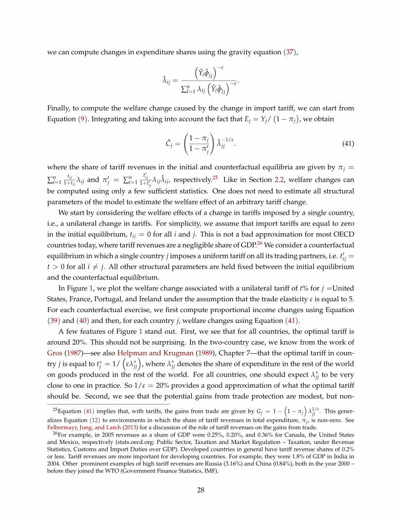
we can compute changes in expenditure shares using the gravity equation (37),

λij =

(Yiφij

)−ε

∑nl=1 λl j

(Yl φl j

)−ε .

Finally, to compute the welfare change caused by the change in import tariff, we can start fromEquation (9). Integrating and taking into account the fact that Ej = Yj/

(1− π j

), we obtain

Cj =

(1− π j

1− π′j

)λ−1/εjj . (41)

where the share of tariff revenues in the initial and counterfactual equilibria are given by π j =

∑ni=1

tij1+tij

λij and π′j = ∑ni=1

t′ij1+t′ij

λijλij, respectively.25 Like in Section 2.2, welfare changes can

be computed using only a few sufficient statistics. One does not need to estimate all structuralparameters of the model to estimate the welfare effect of an arbitrary tariff change.

We start by considering the welfare effects of a change in tariffs imposed by a single country,i.e., a unilateral change in tariffs. For simplicity, we assume that import tariffs are equal to zeroin the initial equilibrium, tij = 0 for all i and j. This is not a bad approximation for most OECDcountries today, where tariff revenues are a negligible share of GDP.26 We consider a counterfactualequilibrium in which a single country j imposes a uniform tariff on all its trading partners, i.e. t′ij =t > 0 for all i 6= j. All other structural parameters are held fixed between the initial equilibriumand the counterfactual equilibrium.

In Figure 1, we plot the welfare change associated with a unilateral tariff of t% for j =UnitedStates, France, Portugal, and Ireland under the assumption that the trade elasticity ε is equal to 5.For each counterfactual exercise, we first compute proportional income changes using Equation(39) and (40) and then, for each country j, welfare changes using Equation (41).

A few features of Figure 1 stand out. First, we see that for all countries, the optimal tariff isaround 20%. This should not be surprising. In the two-country case, we know from the work ofGros (1987)—see also Helpman and Krugman (1989), Chapter 7—that the optimal tariff in coun-try j is equal to t∗j = 1/

(ελ∗jj

), where λ∗jj denotes the share of expenditure in the rest of the world

on goods produced in the rest of the world. For all countries, one should expect λ∗jj to be veryclose to one in practice. So 1/ε = 20% provides a good approximation of what the optimal tariffshould be. Second, we see that the potential gains from trade protection are modest, but non-

25Equation (41) implies that, with tariffs, the gains from trade are given by Gj = 1 −(

1− π j

)λ1/ε

jj . This gener-alizes Equation (12) to environments in which the share of tariff revenues in total expenditure, π j, is non-zero. SeeFelbermayr, Jung, and Larch (2013) for a discussion of the role of tariff revenues on the gains from trade.

26For example, in 2005 revenues as a share of GDP were 0.25%, 0.20%, and 0.36% for Canada, the United Statesand Mexico, respectively (stats.oecd.org: Public Sector, Taxation and Market Regulation – Taxation, under RevenueStatistics, Customs and Import Duties over GDP). Developed countries in general have tariff revenue shares of 0.2%or less. Tariff revenues are more important for developing countries. For example, they were 1.8% of GDP in India in2004. Other prominent examples of high tariff revenues are Russia (3.16%) and China (0.84%), both in the year 2000 –before they joined the WTO (Government Finance Statistics, IMF).

28

0 10 20 30 40 50 60 70 80 90 1000.975

0.98

0.985

0.99

0.995

1

1.005

1.01

1.015

Tariff, %

Wel

fare

cha

nges

rel

ativ

e to

0%

tar

iff r

egim

e

USAFrancePortugalIreland

Figure 1: Welfare changes associated with a unilateral tariff in the country imposing the tariff.Trade elasticity ε = 5. Data are from WIOD in 2008.

trivial. At the optimal tariff, they range from 0.3% for the United States to 1.3% for Ireland. To putthese numbers in perspective, note that the overall gains from trade predicted by the Armingtonmodel for these two countries are 1.8% and 8%, respectively; see Table 1 Column 1. Third, smallercountries that gain more from trade also gain more from optimal trade protection. Here, althoughsmaller countries have less ability to manipulate their terms-of-trade, they benefit disproportion-ately more from an improvement in their terms-of-trade.27 Finally, we see that the range overwhich trade protection is welfare-improving is large. For all four countries, import tariffs up to50% are found to increase real consumption relative to free trade.

Up to this point, we have only focused on welfare changes in the country imposing the importtariff. We now turn to the effects on the rest of the world. We restrict ourselves to a counterfactualscenario in which the United States unilaterally imposes an import tariff of 40% on all its tradingpartners, t′iUS = 0.4 for all i 6=United States. This is close to the tariff level observed in the UnitedStates in the late 19th and early 20th century; see e.g. Irwin (1998). The welfare changes causedby the 40% tariff in each trading partner of the United States are reported in Column 1 of Table 2.The striking feature of these numbers is that in spite of the fact that the United States is the largestcountry in the world (in terms of GDP) and that 40% is a large tariff by historical standards, theimpact on the rest of the world is small. On average, real consumption goes down by 0.2%. Theonly two exceptions are Canada and Mexico, which incur loses of 1.2% and 1.1%, respectively.

The previous counterfactual exercise may mask the true cost of trade protection if other coun-

27In general, one would expect gains from trade protection to have an inverted-U shape as a function of country size,since gains from applying an optimal tariff must go to zero as countries become either infinitesimally small or infinitelylarge. Figure 1 suggests that countries in our dataset are sufficiently large that they are on the declining segment of thiscurve.

29

tries retaliate by increasing their own import tariffs. A very crude way to assess the quantitativeimportance of trade wars is to consider a counterfactual scenario in which all countries, ratherthan one, impose a 40% import tariff on all their trading partners. The associated welfare changesare reported in Column 5 of Table 2. On average, countries experience losses of 2.3%. The biggestloser is Ireland (−4.4%) while the country that loses the least is the United States (−0.8%). In thisparticular counterfactual scenario, no country wins the trade war, though the largest country inthe world is the one that loses the least.

While the previous numbers are illustrative, a more satisfactory way to study the consequencesof trade wars is to solve for the Nash equilibrium of a non-cooperative tariff game. As demon-strated in Ossa (2011b), one can still do so using the exact hat algebra. The only difference betweenthis analysis and the one presented in this section is that proportional changes in trade costs, φij,are no longer exogenously given, but correspond to the best-response of each country to the vectorof import tariffs chosen by its trading partner. Using a multi-sector gravity model with monopo-listic competition and estimates of trade elasticities from Broda and Weinstein (2006), Ossa (2011b)finds Nash tariffs around 60% around the world. Ossa finds that the associated welfare loss asso-ciated with going from the current, observed equilibrium to the counterfactual Nash equilibriumis equal to 3.5% on average.

4.2 Alternative Gravity Models Revisited

In the previous subsection we have focused on the predictions of a simple Armington model. Wenow go back the main gravity models considered in Sections 3.2, 3.3, and 3.4 to see how multiplesectors, intermediate goods, and monopolistic competition affect these predictions. For exposi-tional purposes, we restrict ourselves to counterfactual scenarios in which tariffs are commonacross sectors. We discuss the specific issues associated with heterogeneity in tariffs in the nextsubsection.

We start by allowing for multiple sectors and intermediate goods, in the exact same way as inSections 3.3 and 3.4, while retaining the assumption of perfect competition, δs = 0 for all s. As inSection 4.1, we assume that all tariffs are zero in the initial equilibrium. Columns 2 and 4 in Table2 report the welfare effects of a unilateral 40% tariff imposed by the United States on all its tradingpartner in all sectors. Column 2 corresponds to the predictions of the multi-sector model withoutintermediate goods, αj,s = 0, whereas Column 4 corresponds to the predictions with intermediategoods, αj,s > 0.28 Columns 6 and 7 show the analogous results when the 40% tariff is imposeduniformly by all countries around the world. For both counterfactual scenarios, welfare changesare computed using the exact-hat algebra as we did in the case of the simple Armington model.

Moving from a one-sector to a multi-sector model has ambiguous effects on the welfare lossesfrom a tariff; for many countries we actually see smaller losses. For example, the welfare losses inChina from the 40% worldwide tariff fall from 1.6% in the one-sector model (Column 5) to 0.4% in

28In the latter case, shares of intermediate goods are computed as α∗j,ks =(

∑k ∑i Xij,ks/Rj,s

)×(

Ej,k/Ej

).

30

the multi-sector model (Column 6). On average, welfare losses go from 2.3% (Column 5) to 1.4%(Column 6). Although we know from the results of Section 3.3 that a prohibitive tariff should leadto higher welfare losses when there are multiple-sectors, we see that even for tariffs as high as 40%worldwide, this is not the case. Thus one should be careful when extrapolating from the autarkyexercises of Section 3 to richer comparative static exercises. Models that point towards larger gainsfrom trade liberalization for one counterfactual scenario may very well lead to smaller gains fromtrade liberalization for another.

In contrast, allowing for intermediate goods significantly amplifies the losses generated bytariffs for all countries, echoing the results of Section 3.4. Canada now experiences a welfare lossof 2.3% (Column 4) rather than 1.2% (Column 2) as a consequence of the 40% tariff imposed bythe United States, while average losses are now 0.33% (Column 4) rather than 0.14% (Column 2).A worldwide tariff of 40% now leads to losses in Belgium of 6.3% (Column 7) rather than 2.6%(Column 6). On average, allowing for intermediate goods leads to welfare losses of 3.4% (Column7) rather than 1.4% (Column 6).

We next study how market structure affects the welfare effects of a worldwide tariffs of 40%.As explained in Section 3, moving from perfect to monopolistic competition introduces scale ef-fects, which complicates the computation of counterfactual equilibria with tariffs. To ease thecomputational burden, we use a coarser version of our dataset in all the exercises that follow.Specifically, we aggregate the set of countries in the WIOD into 10 regions and 16 sectors: 15 agri-culture and manufacturing sectors plus 1 service sector; see online Appendix for details. Usingthis coarser dataset, we compare the predictions of gravity models under the assumption of: (i)perfect competition; (ii) monopolistic competition without firm-level heterogeneity, as in Krug-man (1980); and (iii)monopolistic competition with firm-level heterogeneity, as in Melitz (2003).29

In the case of models with monopolistic competition with firm-level heterogeneity, counterfactualpredictions depend on whether fixed exporting costs are paid in the importing country or export-ing country and whether import tariffs are imposed before or after firm-level markups. In whatfollows we assume that fixed exporting costs are paid in the exporting country, cx

ij = Yi, and thattariffs are imposed before markups; see online Appendix for details.30

Columns 1 to 3 of Table 3 present results for the model without intermediates, as in Section 3.3,while Columns 4 to 6 present results for the model with intermediates, as in Section 3.4. Underperfect competition without intermediate goods (Column 1 in Table 3), the welfare losses associ-ated with a 40% worldwide tariff are lower than before (Column 6 in Table 2). This reflects thefact that, by construction, tariffs are now forced to be zero within regions. Column 2 of Table

29We maintain the assumption that the service sector is perfectly competitive. Formally, in cases (ii) and (iii) we setand δs = 1 for all s 6= 16 and δ16 = 0. The only difference is that in case (ii) we set ηs = 0 for all s whereas in case (iii)we set ηs = 0.65 for all s.

30When tariffs are imposed before markups, they act as “cost-shifters.” Under this assumption, the elasticity of bilat-eral trade flows with respect to tariffs and iceberg trade costs coincide. When tariffs are imposed after markups, theyact as “demand-shifters.” Under this assumption, the elasticity with respect to tariffs is equal to ε+ η rather than ε; seeonline Appendix and Felbermayr, Jung, and Larch (2013). Since there is little empirical evidence to help us discriminatebetween these two cases, we prefer working under the assumption that there is only one elasticity.

31

3 shows the analogous results under monopolistic competition without firm-level heterogeneity.As in Section 3.3, the differences between perfect and monopolistic competition arise because ofsector-level scale effects triggered by trade protection. Welfare losses tend to be larger under mo-nopolistic competition than perfect competition, although there are some exceptions, includingNorth America for which losses go from 0.6% to 0.4%. Finally, Column 3 of Table 3 shows the re-sults under monopolistic competition with firm-level heterogeneity. We see that all regions haveslightly lower welfare losses than in the absence of firm-level heterogeneity. One potential expla-nation is that the introduction of tariffs leads to an increase in the ratio of expenditures—whichinclude tariff revenues—to factor prices. This tends to increase the set of varieties available toconsumers when a tariff is imposed in models with firm-level heterogeneity through selection ef-fects. Since consumers love variety, this tends to reduce the welfare losses associated with a tariffin such models.

How are the previous results affected by the introduction of intermediate goods? We againfind that welfare losses from tariffs tend to be larger in models with monopolistic competition.Moving from Column 4 to Column 5 in Table 3, the losses from the tariff for Western Europe andLatin America increase from 1.6% to 7.6% and from 1.5% to 3.1%, respectively. Welfare losses tendto be even larger under firm-level heterogeneity (Column 6 in Table 3). The average welfare lossesincrease from 5.3% to 7.0%. Like in Section 3.4, this reflects stronger scale effects under models ofmonopolistic competition with firm-level heterogeneity.

In recent work Balistreri, Hillberry, and Rutherford (2011) have compared the predictions ofa multi-sector Armington model with intermediate goods to those of a multi-sector Melitz (2003)model with intermediate goods. To compare the two models, they first estimate the structuralparameters of the Melitz (2003) model using non-linear least squares and investigate the welfareconsequences of a 50% reduction in observed tariffs. They then ask what the welfare consequencesof the same tariff change would have been in an Armington model calibrated using the sameelasticity of substitution between goods (but different trade elasticities) and the same variabletrade costs. They find gains from 50% reduction in tariffs that are four times larger accordingto the Melitz (2003) model and conclude that it is important to add firm-level heterogeneity tostandard quantitative trade models.

The similarity between the quantitative results of Balistreri, Hillberry, and Rutherford (2011)and those presented in Table 3 notwithstanding, there are some important methodological differ-ences. In order to demonstrate the importance of firm-level heterogeneity, Balistreri, Hillberry,and Rutherford (2011) compare Armington to Melitz (2003). Here we compare Krugman (1980) toMelitz (2003). To us the latter comparison is preferable to the former since comparing Armingtonand Melitz (2003) makes it impossible to separate the role of monopolistic competition from therole of firm-level heterogeneity. The results of Table 3 illustrate the importance of this distinctionboth qualitatively and quantitatively. When comparing Columns 1 and 3, one would concludethat gains from trade liberalization are larger in models with firm-level heterogeneity. Yet com-paring Columns 2 and 3, we see that the average welfare loss would be even higher in the absence

32

of firm-level heterogeneity. Similarly, when comparing Columns 4 and 6, one would concludethat average welfare losses are almost three times as large. Yet the relevant comparison, Column5 to Column 6, suggests less dramatic differences, with average welfare losses going from 5.3% to7.0%.

The more substantial methodological difference comes from how we calibrate the modelswhose predictions we want to compare. In Balistreri, Hillberry, and Rutherford (2011), differ-ent models do not match the same set of moments, including the trade elasticity. In this chapter,they do. Our view is that whether or not one wants to “recalibrate” models depends on why oneis interested in comparing the predictions of different models in the first place.

The thought experiment that motivates us can be sketched as follows. Consider two tradeeconomists trying to predict the welfare effects of the same tariff change. Both economists haveaccess to the same trade data in 2008, but the first-one has been trained in the 1980s and thinksthat Krugman (1980) is a useful approximation of the world economy, whereas the second hasbeen trained in the 2000s and thinks that Melitz (2003) is. We want to know whether conditional onthe same trade data, the forecasts of the first and second economists would differ. When comparingone model to another, we therefore recalibrate all structural parameters so that each models fitsthe same cross-section of bilateral trade flows and trade elasticity.

The thought experiment behind the results of Balistreri, Hillberry, and Rutherford (2011) isimplicitly different. The idea is to start with one economist, trained in the 2000s, ask for her fore-cast of the effects of trade policy in 2008 and then ask whether she would have made a differentforecast in a counterfactual world without firm-level heterogeneity. This is why Balistreri, Hillberry,and Rutherford (2011) first structurally estimate a Melitz (2003) model and then “turn off” hetero-geneity across firms (among other things).

So which of these two thought experiments is more useful? If the question is how the Melitz(2003) model has changed the evaluation of trade policy, we think that the first thought experimentis the appropriate one and that comparing Column 2 to Column 3 or Column 5 to Column 6in Table 3 is the right way to go. In contrast, if one is interested in decomposing the results ofColumns 3 or 6 so that one can quantify the role of heterogeneity for welfare within the Melitz(2003) model, then the second thought experiment is more useful.

4.3 Heterogeneous Tariffs

In practice, tariffs are not uniform across sectors within the same country. This raises a number ofquestions: Does heterogeneity in tariffs raise the cost of trade protection in the country imposingthe tariffs? If so, is this also true in the countries facing the tariffs? In theory, what is the “right”way to measure the restrictiveness of trade policy when trade policy is a multi-dimensional object?

Let us start by focusing on the first two questions. We use the simplest model in which thesequestions can be addressed: a multi-sector gravity model without intermediate goods and withperfect competition. Thus the assumptions are the same as in Section 3.3 with δs = 0 for all s. Weagain consider the counterfactual scenario in which only one country, the United States, imposes

33

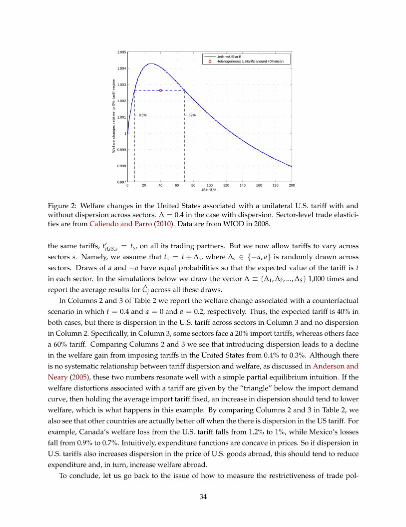
0 20 40 60 80 100 120 140 160 180 2000.997

0.998

0.999

1

1.001

1.002

1.003

1.004

1.005

US tariff, %

Wel

fare

cha

nges

rel

ativ

e to

0%

tar

iff r

egim

e← 8.5% ← 69%

Uniform US tariffHeterogeneous US tariffs around 40% mean

Figure 2: Welfare changes in the United States associated with a unilateral U.S. tariff with andwithout dispersion across sectors. ∆ = 0.4 in the case with dispersion. Sector-level trade elastici-ties are from Caliendo and Parro (2010). Data are from WIOD in 2008.

the same tariffs, t′iUS,s = ts, on all its trading partners. But we now allow tariffs to vary acrosssectors s. Namely, we assume that ts = t + ∆s, where ∆s ∈ −a, a is randomly drawn acrosssectors. Draws of a and −a have equal probabilities so that the expected value of the tariff is tin each sector. In the simulations below we draw the vector ∆ ≡ (∆1, ∆2, ..., ∆S) 1,000 times andreport the average results for Cj across all these draws.

In Columns 2 and 3 of Table 2 we report the welfare change associated with a counterfactualscenario in which t = 0.4 and a = 0 and a = 0.2, respectively. Thus, the expected tariff is 40% inboth cases, but there is dispersion in the U.S. tariff across sectors in Column 3 and no dispersionin Column 2. Specifically, in Column 3, some sectors face a 20% import tariffs, whereas others facea 60% tariff. Comparing Columns 2 and 3 we see that introducing dispersion leads to a declinein the welfare gain from imposing tariffs in the United States from 0.4% to 0.3%. Although thereis no systematic relationship between tariff dispersion and welfare, as discussed in Anderson andNeary (2005), these two numbers resonate well with a simple partial equilibrium intuition. If thewelfare distortions associated with a tariff are given by the “triangle” below the import demandcurve, then holding the average import tariff fixed, an increase in dispersion should tend to lowerwelfare, which is what happens in this example. By comparing Columns 2 and 3 in Table 2, wealso see that other countries are actually better off when the there is dispersion in the US tariff. Forexample, Canada’s welfare loss from the U.S. tariff falls from 1.2% to 1%, while Mexico’s lossesfall from 0.9% to 0.7%. Intuitively, expenditure functions are concave in prices. So if dispersion inU.S. tariffs also increases dispersion in the price of U.S. goods abroad, this should tend to reduceexpenditure and, in turn, increase welfare abroad.

To conclude, let us go back to the issue of how to measure the restrictiveness of trade pol-

34

icy when trade policy is a multi-dimensional object. Anderson and Neary (2005) propose thefollowing two-step approach. First, ask: What is the welfare loss associated with a vector of het-erogeneous tariffs in the country imposing those tariffs? Second, compute the uniform tariff acrosssectors that would lead to the same welfare loss. This number is what Anderson and Neary (2005)refer to as the Trade Restrictiveness Index (TRI). One way to compute this index is to estimate im-port demand elasticities and use linear approximations; see e.g. Feenstra (1995) and Kee, Nicita,and Olarreaga (2008). An alternative is to use the full structure of the model. We now do so againfor the case above with t = 0.4 and a = 0.2. From Table 2 Column 2, we know that the welfarechange in the United States is 0.27%. The Trade Restrictiveness Index can then be read off Figure2, which is the counterpart of Figure 1 in the multi-sector case. In this particular example, thereare two values of the TRI: 8.5% and 69%. The non-uniqueness of the TRI reflects the importanceof general equilibrium effects in gravity models.

5 Numbers We Can Believe In?

5.1 Sensitivity to Auxiliary Assumptions

In Sections 3 and 4 we have studied how different assumptions about technology and marketstructure may affect the welfare consequences of trade liberalization. This exercise already givesus a sense of the sensitivity of the counterfactual predictions of gravity models to a set of keyeconomic assumptions. Here we go one step further by exploring how apparently innocuousauxiliary assumptions may also have large implications for counterfactual analysis.

Nature of Trade Imbalances. All models reviewed in this chapter are static models that aimto capture the long-run consequences of trade liberalization. Given their static nature, all thesemodels predict that trade should be balanced country-by-country. In practice, it is not. Volumesof intertemporal trade are substantial: some countries, like the United States, run large current-account deficits, whereas others, like China, run large current-account surpluses. To deal withtrade imbalances in the context of a static model, the standard approach consists in modellingtrade deficits and surpluses as lump-sum transfers between countries; see e.g. Dekle, Eaton, andKortum (2008). Short of a dynamic theory of trade imbalances, in which today’s trade deficits arepaid back by future trade surpluses, the researcher interested in the effects of a change in tradepolicy has to assume that these lump-sum transfers remain “unchanged” between the initial andthe counterfactual equilibrium.

An obvious question when adopting the previous approach is: “unchanged” compared towhat? When thinking about the U.S. deficit, for instance, should one hold its value fixed relativeto U.S. GDP or World GDP to mention only two of the most natural alternatives? To get a sense ofthe importance of these considerations, let us go back to the Armington model with import tariffsconsidered in Section 4.1. In the presence of trade imbalances across countries, the equilibrium

35

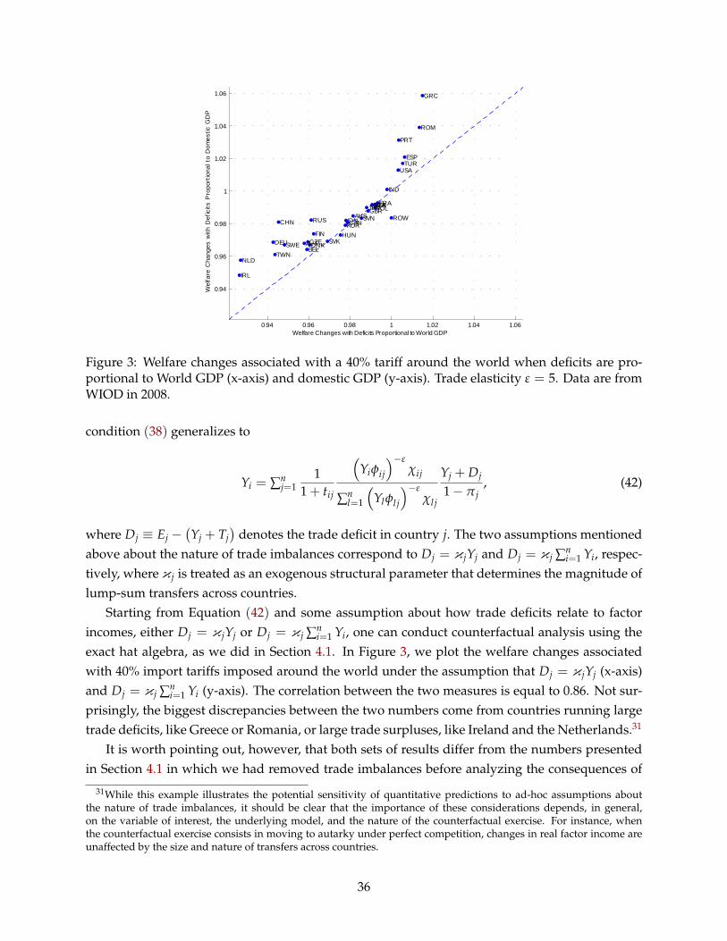
0.94 0.96 0.98 1 1.02 1.04 1.06

0.94

0.96

0.98

1

1.02

1.04

1.06

AUS

AUTBEL

BRA

CANCHN

CZEDEU DNK

ESP

FIN

FRAGBR

GRC

HUN

IDN

IND

IRL

ITAJPN

KOR

MEX

NLD

POL

PRT

ROM

RUS

SVK

SVN

SWE

TUR

TWN

USA

ROW

Welfare Changes with Deficits Proportional to World GDP

Wel

fare

Cha

nges

with

Def

icits

Pro

port

iona

l to

Dom

estic

GD

P

Figure 3: Welfare changes associated with a 40% tariff around the world when deficits are pro-portional to World GDP (x-axis) and domestic GDP (y-axis). Trade elasticity ε = 5. Data are fromWIOD in 2008.

condition (38) generalizes to

Yi = ∑nj=1

11+ tij

(Yiφij

)−εχij

∑nl=1

(Ylφl j

)−εχl j

Yj + Dj

1− π j, (42)

where Dj ≡ Ej −(Yj + Tj

)denotes the trade deficit in country j. The two assumptions mentioned

above about the nature of trade imbalances correspond to Dj = κjYj and Dj = κj ∑ni=1 Yi, respec-

tively, where κj is treated as an exogenous structural parameter that determines the magnitude oflump-sum transfers across countries.

Starting from Equation (42) and some assumption about how trade deficits relate to factorincomes, either Dj = κjYj or Dj = κj ∑n

i=1 Yi, one can conduct counterfactual analysis using theexact hat algebra, as we did in Section 4.1. In Figure 3, we plot the welfare changes associatedwith 40% import tariffs imposed around the world under the assumption that Dj = κjYj (x-axis)and Dj = κj ∑n

i=1 Yi (y-axis). The correlation between the two measures is equal to 0.86. Not sur-prisingly, the biggest discrepancies between the two numbers come from countries running largetrade deficits, like Greece or Romania, or large trade surpluses, like Ireland and the Netherlands.31

It is worth pointing out, however, that both sets of results differ from the numbers presentedin Section 4.1 in which we had removed trade imbalances before analyzing the consequences of

31While this example illustrates the potential sensitivity of quantitative predictions to ad-hoc assumptions aboutthe nature of trade imbalances, it should be clear that the importance of these considerations depends, in general,on the variable of interest, the underlying model, and the nature of the counterfactual exercise. For instance, whenthe counterfactual exercise consists in moving to autarky under perfect competition, changes in real factor income areunaffected by the size and nature of transfers across countries.

36

a worldwide tariff. The correlation between either one of the two measures presented here andthe results of Section 4.1 is 0.57. This discrepancy is caused by larger terms-of-trade improve-ments for countries that maintain large trade deficits. Intuitively, as tariffs increase, consumershave incentives to substitute away from foreign goods towards domestic goods. Thus, in orderto maintain trade deficits “unchanged” in the counterfactual equilibrium, domestic prices mustincrease relative to the price of foreign goods.

Nature of Physical Capital. In earlier sections we have implicitly treated physical capital as aprimary factor of production whose endowment is fixed and unaffected by trade. Alternatively,one could think of physical capital as capital goods that, like other intermediate goods, are tradedinternationally; see e.g. Eaton and Kortum (2001). To get a sense of how important this assumptionon the nature of physical capital could be, we come back to the model of Section 3.4 with multiplesectors, tradable intermediate goods, and perfect competition. Compared to the analysis of Section3.4, the only difference is that we adjust value-added shares in the data so that the (presumed) onethird share of capital in value added is distributed proportionally among intermediate goods fromall industries. Formally, we adjust shares by setting α′i,ks = αi,ks

(1+ 1

31−αi,s

αi,s

). By construction, the

new value added share is therefore two thirds of the one reported in the data: 1− α′i,s =23 (1− αi,s).

When physical capital is treated as another tradable intermediate goods, the amplification effectfrom the input-output loop discussed in Section 3.4 is now stronger, and the gains are larger. Usingagain WIOD data from 2008, we find that average gains from trade are equal to 34.6% comparedto 26.9% when physical capital is assumed to be immobile across countries. For example, gainsfrom trade in Canada are now 36.9% rather than 30.2%, and in the United States they are 11.3%rather than 8.3%.

5.2 Goodness of Fit

One way to try to build confidence in the predictions of gravity models is to assess whether theycan match cross-sectional or time-series evidence on bilateral trade flows.

Cross-sectional Evidence. A standard practice in the literature consists in assuming first that ice-berg trade costs τ are deterministic functions of various observables such as physical distancebetween country i and country j, whether country i and j share a common border or language,or whether they are part of a regional trade agreement or a monetary union. Once trade costfunctions—together with other structural parameters of the model—have been estimated or cali-brated, one can assess the goodness of fit of the gravity model by comparing trade flows predictedby the model to those that are observed in the data; see e.g. Di Giovanni and Levchenko (2009),Waugh (2010), and Fieler (2011).

The empirical fit of gravity models tends to be very good; see Anderson (2010). It is not clear,however, whether this should make us very confident in the counterfactual predictions of thesemodels. If iceberg trade costs τ are used as free parameters, then gravity models can replicateany cross-section of bilateral trade flows, X. Thus, one way to interpret the good fit of the gravity

37

models under particular restrictions on the structure of iceberg trade costs is that these restrictedtrade costs are good proxies of the “wedges” that are necessary for the model to match the data.

An alternative strategy, in the spirit of the test of Heckscher-Ohlin-Theorem in Trefler (1993), isto infer from the trade data the iceberg trade costs such that gravity models fit perfectly and thencheck whether the inferred iceberg trade costs match observable measures of trade costs such astariffs and freight costs or price gaps (which should reflect trade costs under perfect competition).An issue with this approach is that one cannot separately identify iceberg trade costs from country-specific biases in preferences in the model. If “wedges” only match observed measures of tradecosts very imperfectly, should we conclude that there is a problem with the model or that biasesin preferences are important?

In recent work, Anderson and Yotov (2012) propose to test gravity models by focusing onthe restrictions that it imposes on the relationship between exporter- and importer-fixed effectsin equation (13), whatever the structure of iceberg trade costs may be. Another possible strategyto assess the goodness of fit of quantitative trade models consists in using other, i.e. non-trade,data sources. For instance, since gravity models offer a mapping between trade data and con-sumer price indices, one could compare the prices predicted by the model to those observed inthe data. Waugh (2010) and Fitzgerald (forthcoming) offer two examples of papers exploring theimplications of gravity models for prices.

Time Series Evidence. Perhaps the most direct way to test the predictions of a gravity model is tocalibrate the model in a baseline year t, consider a change in trade costs between the baseline yeart and some other year t′, and report the “distance” between the predictions of the model and thedata at date t′.

A natural candidate for large changes in trade costs are regional trade agreements like theNorth American Free Trade Agreement (NAFTA). Caliendo and Parro (2010) use a multi-sectorversion of Eaton and Kortum (2002) with intermediate goods calibrated to match trade data from1993 to study the effects of NAFTA. This model is a special case of the models considered in Section3.4 in that it does not feature any scale effects: δs = 0 for all s. After feeding tariff changes causedby NAFTA between 1993 and 2005, they find that the simulated changes can account for 93% ofthe observed change in Mexico’s total trade over GDP, 58% for Canada, and 55% for the UnitedStates.

The relatively good fit of their model contrasts with the fairly poor performance of earlier CGEmodels reviewed in Kehoe (2005). He evaluates the performances of three of the most promi-nent multisectoral applied general equilibrium models used to predict the impact of NAFTA:the Brown-Deardorff-Stern model of all three North American economies (Brown, Deardorff, andStern (1992)), the Cox-Harris model of Canada (Cox and Harris (1992)) and the Sobarzo model ofMexico (Sobarzo (1992)). He finds that each of these models drastically underestimated the impactof NAFTA on trade volumes. For instance, the Brown-Deardorff-Stern model predicts changes inexports relative to GDP between 1988 and 1999 equal to 50.8% for Mexico, 4.3% for Canada, and2.9% for the United States. In the data, these changes are equal 140.6%, 52.9%, and 19.1%, respec-

38

tively.It is not entirely clear, however, what accounts for the difference in the performance between

more recent and older CGE models. Caliendo and Parro (2010) emphasize the importance ofinput-output linkages for their results, but such linkages are already present in older CGE mod-els. One economically meaningful difference is that the previous CGE models feature imperfectcompetition and scale effects, whereas Caliendo and Parro (2010) does not. But there are manyother potential sources of discrepancies, from the calibration of the trade elasticities (more on thatbelow) to the choice of the baseline year. Indeed, although the predictions of the models reviewedin Kehoe (2005) are compared with changes in the data over the period 1988-1999, the Brown-Deardorff model was calibrated to a 1976 input-output matrix for Canada, a 1980 input-outputmatrix for Mexico, and a 1977 input-output matrix for the United States. The good fit of gravitymodels in the time-series is also called into question by the results of Lai and Trefler (2002) whofind that changes in tariffs between 1972 and 1992 fed into a simple model à la Krugman (1980)can explain little of the variation in bilateral trade flows over this time period.

A poor fit of a quantitative trade model may always reflect the fact that the trade shock understudy is small compared to other unobserved shocks—e.g. technology, factor endowments—thatmay have been occurring over the same time period. This generates a tension. One would want tofocus on shorter time periods around a particular episode of trade liberalization to exclude othershocks, but quantitative trade models are static models that are better equipped to capture thelong-run consequences of trade liberalization than short-term dynamics. In the case of NAFTA,for instance, would quantitative trade models perform better when the final year is 1995, 2000, or2005?

Donaldson (2008) offers an innovative way to test the predictions of gravity models. He fo-cuses on one of history’s great transportation projects: the network of railroads built in colonialIndia from 1870 to 1930. He first estimates the impact of the railroad on trade costs using infor-mation about price gaps across Indian districts. He then feeds the observed changes in trade costsinto a multi-sector version of Eaton and Kortum (2002)—a special case of the models consideredin Section 3.3 without scale effects: δs = 0 for all s—to predict the changes in real income acrossIndian districts. The test of the model comes from comparing changes in real income predictedby the model to the reduced-form estimates of changes in real income caused by the railroad. Hefinds that 86% of the total impact of the railroads on real income in an average district can beexplained by the model.

5.3 Calibrating Elasticities

The key parameters for counterfactual analysis using gravity models, like other CGE models, areelasticities. We conclude this section by discussing some of the issues arising when calibratingelasticities.

Trade Elasticities. As can already be seen from the counterfactual analysis carried in the contextof the Armington model in Section 2, the single most important structural parameter in gravity

39

models is the trade elasticity. Conditional on observed trade shares, it determines both the re-sponse of bilateral trade flows and real consumption. In more general environments such as thoseconsidered in Section 3, it remains one of the key statistics required to estimate the gains frominternational trade; see Equations (23), (27), and (32). So, how large are trade elasticities?

This question is an old one. It is as important for recent gravity models reviewed in this chapteras for earlier CGE models. The broad consensus in the CGE literature is, in the words of Dawkins,Srinivasan, and Whalley (2001), that “the quantity and quality of literature-based elasticity para-meters for use in calibrated models is another Achilles’ heel of calibration.” As John Whalley notes“It is quite extraordinary how little we know about numerical values of elasticities [...] In the in-ternational trade area researchers commonly use import price elasticities in the neighborhood ofunity, even for small economies, even though elasticity estimates as high as nine appear in theliterature.” The same pessimism can be found in the review of trade elasticities by McDaniel andBalistreri (2003): “The estimates from the literature provide a wide range of point estimates, andlittle guidance on correct estimates to apply to a given commodity in a given model for a givenregional aggregation. Most of the controversy surrounding the [trade] elasticities reduces to ageneral structural inconsistency between the econometric models used to measure the responseand the simulation models used to evaluate policy.”

Part of the success of new quantitative work in international trade lies in the tight connectionbetween the structural estimation of the trade elasticity and the underlying economic model. Intheir seminal work, Eaton and Kortum (2002) offer multiple ways to estimate structurally the tradeelasticity using a gravity equation akin to Equation (16). Their estimates range from ε = 3.60 toε = 12.86 with a preferred value of ε = 8.28 when using price gaps as a measure of trade costs.While the range is wide, it remains in the range of elasticities used in earlier CGE models; seeHertel (1997). In recent work, Simonovska and Waugh (2011) refine Eaton and Kortum (2002)’spreferred estimation strategy to take into account the fact that price gaps are only lower-boundson trade costs. Simonovska and Waugh (2011) propose a simulated method of moments to correctfor the fact that trade elasticities using price gaps tend to overestimate the sensitivity of tradeflows to trade costs. Their preferred estimate of ε is 4.12.

The merits of a tight connection between theory and data notwithstanding, the state of affairsremains far from ideal. An issue with simulation using earlier CGE models, such as those usedin the evaluation of NAFTA, is that they require a very large number of elasticities. Many recentpapers, following Eaton and Kortum (2002), side-step this issue by assuming that all goods enterutility functions through a unique CES aggregator. But empirically, there is ample evidence ofsignificant variation in the trade elasticity across sectors; see e.g. Feenstra (1994), Broda and We-instein (2006), and Hummels and Hillberry (2012). If so, why should we be more confident in thecounterfactual predictions of simpler gravity models that abstract from this heterogeneity? Giventhe heterogeneity in the trade elasticity across sectors, is the trade elasticity estimated from anaggregate gravity equation like (16) the “right” trade elasticity to calibrate a one-sector model?32

32Imbs and Mejean (2011) argue that such aggregate trade elasticities suffers from heterogeneity bias and that one

40

A natural way to address the previous concerns is to write down multiple-sector models, suchas those considered in Section 3.3, and incorporate formally the heterogeneity in trade elasticitiesacross sectors. But this raises new issues. As the number of elasticities that needs to be esti-mated increases, the precision with which each of those elasticities is estimated tends to decrease.Accordingly, results become much more sensitive to the presence of outliers. To take a concreteexample, the sector-level elasticities from Caliendo and Parro (2010) used in Section 3.3 are around8 on average. But for some sectors, like automobiles, trade elasticities are not statistically differentfrom zero. An elasticity of zero would imply infinite gains from trade.33

Upper-level Elasticities (I): Substitution Across Sectors. Going from a one-sector to a multi-sector model raises another question: How large is the elasticity of substitution between sectors?All papers referenced in Section 3.3 follow what Dawkins, Srinivasan, and Whalley (2001) referto as the “idiot’s law of elasticities”: all elasticities are equal to one until shown to be otherwise.How important is the assumption that upper-level utility functions are Cobb-Douglas for the pre-dictions of multi-sector quantitative trade models?

To shed light on this question, let us make the same assumptions as in Section 3.3, expect forthe fact the upper-level utility function is now given by

Cj =(

∑Ss=1 βj,sC

(γ−1)/γj,s

)γ/(γ−1), (43)

where γ > 0 denotes the upper-level elasticity of substitution between goods from different sec-tors; βj,s ≥ 0 are exogenous preference parameters, which we normalize such that ∑S

s=1 βj,s = 1for all j; and Cj,s still denotes total consumption of the composite good s in country j. The Cobb-Douglas case studied in Section 3.3 corresponds to γ = 1.

For simplicity let us focus on the case of perfect competition, δs = 0 all s. Following a pro-cedure similar to that in Section 3.1, one can show that if sector-level price indices are given byEquation (20), then the welfare impact of a shock generalizes to

Cj =

(∑S

s=1 ej,s

(λ−1jj,s

)(γ−1)/εs)1/(γ−1)

. (44)

Gains from trade are thus given by

Gj = 1−(

∑Ss=1 ej,s

(λjj,s

)(γ−1)/εs)1/(γ−1)

. (45)

In Section 3.3, we have pointed out that multi-sector models with Cobb-Douglas preferences pre-dict significantly larger gains than one-sector models. Using Equation (45), we can now quantify

should instead use a properly weighted average of sector-level trade elasticities to calibrate one-sector models. Yet ifthe true model is indeed a multi-sector model, it is not a priori obvious that there exists a single weighted average—independently of how weights are defined—that can be used to predict both changes in trade flows and welfare.

33The existing literature rarely reports confidence intervals. Two notable exceptions are Lai and Trefler (2002) andShapiro (2012) who use the standard errors of the trade elasticities that they have estimated to compute, and report, thestandard errors for the gains from trade liberalization.

41

0 1 2 3 4 5 6 7 80

5

10

15

20

25

30

35

40

45

50

Elasticity of substitution across sectors, γ

Gai

ns f

rom

tra

de,

%

CanadaGermanyFranceJapanUSAAverage for the World

Figure 4: Gains from Trade computed according to Equation (45) for different levels of γ. Sector-level trade elasticities are from Caliendo and Parro (2010). Data are from WIOD in 2008.

the importance of the Cobb-Douglas assumption for this prediction. In Figure 4 we plot Gj as afunction of γ using (45) for several countries—the United States, Canada, France, Germany, andJapan—as well as the average Gj for all countries considered in Table 1. We see that the value of theupper-level elasticity γ—for which the existing empirical literature provides little guidance—haslarge effects on the magnitude of the gains from trade. As we go from the Leontief case, γ = 0, tothe Cobb-Douglas case, γ = 1, to an upper-level elasticity equal to the average of lower-level elas-ticities, γ = 8, average gains from trade decrease from 45% to 15% to 3%.34 The intuition is simple.If the elasticity of substitution between sectors is high, then the consequences of autarky are mit-igated by consumers’ ability to substitute consumption away from the most affected sectors,i.e.,those with lowest values of λ1/εs

jj,s , towards the least affected sectors, i.e., those with highest values

of λ1/εsjj,s . By the same token, however, the gains from further trade liberalization would tend to be

higher with a higher γ, since consumers could more easily reallocate their consumption towardsgoods that experience larger price declines.35

34In the particular case in which all lower-level trade elasticities are equal to the upper-level trade elasticity, εs = γ− 1for all s, the discrepancy between the predictions of multi-sector and one-sector models disappears: Equation (45)reduces to Equation (12).

35The value of the upper-level elasticity of substitution also has more subtle implications for quantitative trade mod-els with monopolistic competition. Away from Cobb-Douglas preferences, expenditure shares ej,s are no longer con-stant, which may lead to multiple equilibria. Intuitively, a higher expenditure share in a given sector lead to moreentry, which reduces the price index in that sector, thereby leading to a higher expenditure share. Thus, one may obtaindifferent estimates of the gains from trade—or the effect of trade policy—depending on the counterfactual equilibriumone focuses on. Another issue concerns the difference between the predictions of models with firm-level heterogeneity,like Melitz (2003), and those without, like Krugman (1980). In Section 3.3, we have shown that in the Cobb-Douglascase, entry effects lead to a distinction between the predictions of models with perfect and monopolistic competition,but not between models with and without firm-level heterogeneity. This is no longer true in the case of general CES

42

Upper-level Elasticities (II): Domestic versus Foreign. Another, and perhaps deeper issue re-garding gravity estimates of the trade elasticity is that they capture the elasticity of substitutionbetween foreign sources of imports. Yet, the elasticity that one needs, for instance, for measur-ing the gains from trade is the elasticity of substitution between home and import goods. To seethis formally, let us go back to the simple Armington model presented in Section 2.1, but let usgeneralize Equation (1) so that

Cj =

[(Cjj)(γ−1)/γ

+(

CMj

)(γ−1)/γ]γ/(γ−1)

,

where CMj measures total consumption of imported goods,

CMj =

(∑i 6=j ψ

σ/(σ−1)ij C(σ−1)/σ

ij

)σ/(σ−1).

The upper-level elasticity γ > 1 now represents the elasticity of substitution between the domes-tic good and the composite of the foreign goods, whereas the lower-level elasticity σ > 0 stillrepresents the elasticity of substitution between foreign goods. The simple Armington model cor-responds to the special case, γ = σ. Under this new demand system, bilateral trade flows stillsatisfy a gravity-like equation:

Xij =

(PM

j

Pj

)1−γ(Pij

PMj

)1−σ

Ej, for all i 6= j, (46)

where Pij = τijPii is the price of goods from country i in country j; PMj ≡

(∑i 6=j ψ1−σ

ij P1−σij

)1/(1−σ)

is the import price index; and Pj =

((Pjj)1−γ

+(

PMj

)1−γ)1/(1−γ)

is the consumer price index in

country j. In this more general environment, one can still rearrange bilateral trade flows as we didin Equation (13) and use the cross-sectional variation in trade flows and trade costs to estimate1− σ.

Now, like in Section 2.2, consider a small change in trade costs that affects country j. Thechange in the consumer price index is still given by

d ln Pj = λjjd ln Pjj +(1− λjj

)d ln PM

j .

But our new demand system now implies

d ln(1− λjj

)− d ln λjj = (1− γ)

(d ln PM

j − d ln Pjj

).

utility functions.

43

Following the same strategy as in Section 2.2, one can therefore show that

d ln Cj = d ln λjj/ (1− γ) . (47)

While gravity estimates can uncover the lower-level elasticity, σ, Equation (47) shows that theupper-level elasticity, γ, i.e., the elasticity of substitution between domestic and foreign goods, isthe relevant elasticity for welfare analysis.36

In standard gravity models, it is only the assumption of symmetric CES utility that allow re-searchers to go from the commonly estimated elasticity, σ, to the welfare-relevant elasticity, γ.When estimated, does the elasticity of substitution between home and import goods, γ, look sim-ilar to the elasticity of substitution between foreign goods, σ? Head and Ries (2001) suggest thatthe answer is yes. They measure the average of the elasticity of demand for Canadian goods inCanada relative to U.S. goods and the elasticity of demand for U.S. goods in the United Statesrelative to Canadian goods. If all trade was U.S.-Canada trade, their estimate would thereforeprovide an estimate of γ. They find an average elasticity equal to 7.8, quite in line with previousgravity estimates of σ. Likewise, using the methodology of Feenstra (1994) to estimate both γ andσ, Feenstra, Obstfeld, and Russ (2013) cannot reject the null that γ and σ are equal.

Factor Supply Elasticities. The multi-sector gravity models that we have reviewed assume aperfectly-elastic factor supply to each sector. Thus, except for the case with sector-level differencesin factor intensities considered in Section 3.5, the aggregate production possibilities frontier (PPF)is linear. In practice one may expect factors to be imperfect substitutes across sectors. For instancesome workers may have a comparative advantage in particular sectors, as in a Roy-type model, orsome natural resources may be critical inputs to production in some sectors and not others. Suchconsiderations would lead to more “curvature” in the PPF and, conditional on observed tradeflows, larger gains from trade.

To take an extreme example, consider the petroleum sector. The trade elasticity, εs, for thissector estimated by Caliendo and Parro (2010) is around 70. The formula presented in Section 3.3would therefore predict very small gains from trade in this sector. Yet, of course, one would expectmany oil importing countries to face enormous losses from moving to autarky. One simple way tocapture such considerations would be to go back to the multi-factor model presented in Section 3.5and assume factors employed in the petroleum sector are specific to that sector, effectively makingpetroleum an endowment. To explore the quantitative importance of this type of considerations,we have recomputed the gains from trade in the multi-factor model under the assumption thatall sectors are perfectly competitive and all factors are sector-specific.37 In line with the previousdiscussion, we find larger gains from trade under the assumption that factors are sector-specific,with the cross-country average for Gj going from 15.3% to 17.2%.

36In more general gravity models, this upper-level elasticity γ would remain a key determinant for welfare analysis,though not the only one.

37Formally, this amounts to using the formula for gains from trade given by Equation(32) under the assumption thatδs = 0 and cA

j,s = ej,s/rj,s for all s.

44

Other Elasticities: Love of Variety and Extensive Margin. We conclude by discussing the cal-ibration of the elasticity of substitution, σ, and the extensive margin elasticity, η, introduced inEquation (15) and its sector-level counterparts, Equations (20), (26), and (30). Given estimates ofthe trade elasticity, ε, these two elasticities are irrelevant for welfare analysis under perfect compe-tition. Under monopolistic competition, however, we have seen that in the presence of intermedi-ate goods, as in Section 3.4, or in multi-sector models with general CES preferences, as discussedabove, the values of σ and η do matter above and beyond the value of the trade elasticity, ε. Inthese richer environments, the predictions of models with and without firm-level heterogeneityare different and the magnitude of the difference crucially depend on how σ and η are calibrated.

As shown in Section 3.2, the three elasticities ε, σ, and η are not independent of one another.In gravity models, ε determines the overall response of trade flows to changes in trade costs,whereas σ − 1 determine their responses at the intensive margin and η =

(ε−(σ−1)

σ−1

)determines

their response at the extensive margin, ε− (σ− 1), weighted by the love of variety, σ− 1. Given anestimate of the trade elasticity, ε, one therefore only needs an estimate of σ to compute η and viceversa. The most direct way to estimate σ or η is to use firm-level trade data; see e.g. Crozet andKoenig (2010) and Eaton, Kortum, and Kramarz (2011). When available, they offer a simple way toestimate the intensive margin elasticity, i.e., by how much the sales of a given set of firms respondto changes in trade costs, and the extensive margin elasticity, i.e., by how much the number offirms responds to changes in trade costs.38 Eaton, Kortum, and Kramarz (2011) estimate a valueof 1.5 for η in a one sector model, whereas Crozet and Koenig (2010) obtain estimates of εs and ηs

for several sectors. Interestingly, the average ηs across s estimated by Crozet and Koenig (2010) isalso 1.5, with little variation across sectors.39

Balistreri and Rutherford (2012) nicely illustrates the issues inherent to the calibration of mod-els of monopolistic competition. The authors compare the predictions of a model without firm-heterogeneity, like Krugman (1980), to those of a model with firm-heterogeneity, like Melitz (2003),in a model with identical countries, three sectors, nested CES preferences, but no inter-industrytrade, ej,s = rj,s. Changes in real consumption are given by Equation (22). Using the fact that

ηs =(

εs−(σs−1)σs−1

), one can show that the overall scale effects,

(eηs

j,srj,s

)δs/εs, are equal to

(rj,s)1/(σs−1)

in the two models. Thus the only difference between the predictions of the two models comesfrom the different values of σs used in the calibration of the two models. In their calibration, Bal-istreri and Rutherford (2012) assume that εs is equal to 4.6 in both models, but that ηs is equalto 0 in the Krugman-version and 0.65 in the Melitz-version. This implies calibrated values of

38A related, though distinct way to estimate the relative importance of the intensive margin, σ− 1, consists in usingthe prevalence of zeros in aggregate trade data; see Helpman, Melitz, and Rubinstein (2008). The obvious drawbackof this approach is that gravity models, in general, do not allow for zeros, therefore creating a tension between thestructural model used for counterfactual analysis and the way its parameters are estimated; see Eaton, Kortum, andSotelo (2012) for recent work on this topic. Alternatively, one can rely more heavily on the overall structure of the modeland use other firm-level measures, like sales and markups, to estimate ε and σ; see e.g. Di Giovanni and Levchenko(2009) and Hsieh and Ossa (2011). Once ε and σ are known, η can then be computed as a residual.

39This value is much larger than the value of ηs = 0.65 used in Section 3.4. If one were to use ηs = 1.5 rather than0.65 when computing the gains from trade using Equation (29), one would conclude that gains from trade predictedby models of monopolistic competition with firm-level heterogeneity cannot be finite for any country in our dataset.

45

σs = εs/ (1+ ηs) + 1 equal to 5.6 in the Krugman-version and 3.8 in the Melitz-version. This leadsto stronger love of variety and, in turn, larger entry effects and gains from trade liberalization inthe latter model. The question, of course, is whether one should take seriously that love of vari-ety is much stronger than previously thought because the intensive margin is only one particularmargin of adjustment of trade flows, σs − 1 < εs, in models with firm-level heterogeneity.

6 “Micro” versus “Macro” Numbers

Our chapter so far has described what could be referred to as a “macro” approach to quantifyingthe consequences of globalization. The distinguishing features of this approach can be summa-rized as follows. First, it aims to study the overall welfare gains from trade. Second, it is based oncommonly available aggregate trade data and a few key structural parameters. Third, it tries toremain agnostic about micro-theoretical foundations. These foundations only matter to the extentthat they affect “macro” aggregates, as illustrated, for instance, in Equations (15) and (16).

A common alternative in the literature consists in following a “micro” approach, more closelyrelated to demand and production function estimation in Industrial Organization. Unlike the“macro” approach described in this chapter, the “micro” approach typically focuses on one par-ticular source of gains from trade using micro-level data, either at the product or firm-level. Thetwo most prominent examples of “new” sources of gains from trade emphasized in this literatureare: (i) gains from new varieties and (ii) productivity gains. The broad objective of this sectionis to discuss how empirical evidence related to (i) and (ii), i.e., “micro” numbers, relate to thepredictions of quantitative trade models reviewed in this chapter, i.e., “macro” numbers.

6.1 Gains From New Varieties

One of the hallmarks of the “new trade theory” pioneered by Paul Krugman in the early 80s isthat consumers may gain from trade through access to new varieties. These may be direct gainscoming from trade in final goods, as in Krugman (1979) and Krugman (1980), or indirect gainscoming from trade in intermediate goods, as in Ethier (1982b). An important contribution of theempirical trade literature in the last decade is to put a number on the “new-goods” channel; see e.g.Klenow and Rodríguez-Clare (1997), Broda and Weinstein (2006), Arkolakis, Demidova, Klenow,and Rodríguez-Clare (2008), Feenstra and Weinstein (2010), and Goldberg, Khandelwal, Pavcnik,and Topalova (2009).

In order to illustrate the similarities and differences with the “macro” approach of this chapter,we will focus on the most influential paper in the “micro” approach: Broda and Weinstein (2006).The starting point of this paper is the observation that statistical agencies typically ignore gainsfrom the creation of new varieties (and destruction of old varieties), when computing variouscomponents of the Consumer Price Index (CPI), including the Import Price Index. The authorsthen go on to ask: How different would measured changes in the Import Price Index of the UnitedStates be if one were to take into account the creation and destruction of varieties over time?

46

To answer this question, the authors first need to define what the counterpart of a varietyin theory is in the data and then to specify a demand system to evaluate the welfare impact ofnew varieties. Broda and Weinstein (2006) define a variety as a 10-digit HTS product from agiven country, e.g. “Umbrellas and Sun Umbrellas Having a Telescopic Shaft from China,” andassume nested CES utility functions like in the present chapter. Given these assumptions, thecontribution of appearing and disappearing varieties to the import component of the CES priceindex, i.e., the expenditure function of a representative US consumer, can then be computed usingan estimate of the elasticity of substitution across foreign varieties and measures of the changesin the share of expenditures on continuing varieties as in Feenstra (1994). The main finding ofBroda and Weinstein (2006) is that, between 1972 and 2001, the decrease in the Import Price Indexassociated with the expansion of imported varieties, and omitted by statistical agencies, has leadto an additional 2.6% decrease in the U.S. CPI.

It should be clear that in spite of its use of micro-level data, the empirical strategy of Broda andWeinstein (2006) has a lot in common with the approach presented in earlier sections of this chap-ter. First, the focus is squarely on welfare, i.e. money metric indirect utility function that are con-structed by means of the expenditure function. Second, the analysis heavily relies on functionalform assumptions, namely CES utility. In particular, the correction term introduced by Feenstra(1994) is closely related to our welfare formula in the simple Armington model; see Equation (9).The basic idea is that under CES utility, changes in relative prices can be inferred from changesin relative expenditure modulo the elasticity of substitution. This is true regardless of whetherchanges in relative prices are due to movements in the price of existing goods or the creation ofnew goods, a fact that we have exploited more generally in Section 3.1.

There is, however, a number of notable differences. A benefit of the “micro” approach takenby Broda and Weinstein (2006) is that it only requires assumptions on the demand system, whichtogether with data on prices and quantities, are sufficient to compute changes in the Import PriceIndex of a representative consumer with nested CES utility. These “micro” numbers are inde-pendent of technological considerations and market structure. In contrast, the “macro” numberspresented in this chapter do heavily depend on functional form assumptions on the supply-sideof the economy, e.g. Fréchet distributions of productivity under perfect competition or Paretodistributions under monopolistic competition.

The previous observation does not imply that technological considerations and market struc-ture are irrelevant for such empirical micro studies. This is best illustrated by the followingthought experiment. Suppose first, as Broda and Weinstein (2006) do in the last part of their analy-sis, that Krugman (1980) is an accurate description of the world. Then changes in the Import PriceIndex due to new varieties should be reflected one-for-one in the overall CPI. Under this assump-tion, “micro” numbers indeed measure additional welfare gains. Now suppose instead that Eatonand Kortum (2002) or some other Ricardian model is an accurate description of the world. Thereis a priori nothing in the trade data that Broda and Weinstein (2006) look at that would contradictthis view of the world. Yet, under this alternative assumption on market structure and technol-

47

ogy, changes in the Import Price Index due to the creation of new varieties should be exactly offsetby changes in the domestic component of the CPI due to the destruction of old varieties. In thisneoclassical world, the set of goods available to consumers is fixed. So the “new-goods” channelis rightly ignored by statistical agencies: in net, it should have no welfare effect. To put it bluntly,“micro” numbers are unaffected by assumptions on technology and market structure, but whetheror not one should care about these numbers crucially depend on these assumptions.40

Another important difference between the “micro” approach taken by Broda and Weinstein(2006) and the “macro” approach presented in this paper is that, at its core, the “micro” approachis a measurement exercise, not a counterfactual exercise. The goal is to document what actuallyhappened in the data, e.g. in the United States between 1972 and 2001, not what could havehappened if China had grown at a different rate or if the United States had chosen different tradepolicies. To address such counterfactual questions, one again needs the full structure of the model;specifying and estimating a demand system is not enough.

6.2 Productivity Gains

In the canonical model of trade with firm-level heterogeneity developed by Melitz (2003), tradeliberalization causes a reallocation of resources from the least to the most productive firms. Thistheoretical prediction has received considerable support in the data, with many empirical studiesfinding very large effects of trade on measured productivity. For instance, Trefler (2004) finds thatthe reallocation of market shares across firms following the Canada-US free trade agreement hascaused productivity, measured as real value added per hour worked, to go up by 8.4% in Canadianmanufacturing. Using the methodology of Olley and Pakes (1996) to measure productivity at thefirm-level, Pavcnik (2002) documents productivity gains of the same order of magnitude followingthe trade liberalization of the manufacturing sector in Chile.

The goal of this subsection is to clarify the relationship between productivity studies and thebody of work reviewed in this chapter. Given space constraints, we will make no attempt at sys-tematically reviewing this large empirical literature; see e.g. Tybout (2001), Melitz and Trefler(2012), as well as Melitz and Redding (2013) in this volume for excellent overviews. Here we willfocus on the following conceptual issues: What is the difference between productivity and wel-fare? If welfare and measured productivity simultaneously go up, should we think of productivitygains as a new source of gains from trade? At a qualitative level, should we always expect welfareand measured productivity to go in the same direction? At a quantitative level, can we directlycompare the “micro” numbers from productivity studies with the “macro” numbers presentedearlier in this chapter?

In theory, productivity measures how much “output” one can produce with a given amount of“input,” whereas welfare measures how much “consumption” one can afford. At the macro level,

40A similar issue arises if one believes that Melitz (2003) rather than Krugman (1980) is an accurate description ofthe world. In this case, however, changes in the Import Price Index and the domestic component of the CPI due to thecreation and destruction of varieties only exactly cancel out under special circumstances, as discussed in footnote 12.

48

the two concepts are therefore closely related. In a closed economy, the more productive a countryis, the more it can produce, and so, the more it consumes. This is why real GDP computed onthe revenue and expenditure sides coincide. In an open economy, the two concepts differ becauseof terms-of-trade effects. Absent any shock to a country’s productivity, a country may be ableto consume more if it can purchase more imports with the same amount of exports, i.e., if itsterms-of-trade improve.

An obvious, but important difference between the results in this chapter and productivitystudies therefore lies in the treatment of terms-of-trade effects. They are central to our analysis.In the simple Armington model, like in any neoclassical model, terms-of-trade effects are the onlychannel through which foreign shocks may affect welfare in another country. One of the maingoals of quantitative trade models therefore is to predict the terms-of-trade changes associatedwith particular shocks. In contrast, terms-of-trade effects play no direct role in productivity stud-ies, whose main goal is to identify the consequences of trade liberalization on productivity at thefirm- and industry-level.

For the rest of our discussion, let us set aside the issue of terms-of-trade effects. The exact re-lationship between measured productivity and welfare depends, of course, on how one measuresproductivity as well as the model used to compute welfare; see Burstein and Cravino (2011) for ageneral discussion. For our purposes here, let us simply assume that all firm-level data are con-sistent with Melitz (2003) and that industry-level measures of productivity (in the data) increaseswhenever the distribution of firm-level productivity (in the model) shifts to the right.41 Even un-der such ideal circumstances, changes in measured productivity caused by reallocations acrossfirms and welfare may be quite different, as we now illustrate through a series of short examples.

Consider first a small decrease in variable trade costs. The decrease in variable trade costs,which can be thought of as an outward shift in the production possibility frontier, will lead to adirect first-order increase in welfare. In addition, there will be a reallocation of resources fromthe least to the most efficient firms, and this will lead to an increase in measured productivity atthe industry level. Since the initial equilibrium is efficient under monopolistic competition withCES utility, see e.g. Dhingra and Morrow (2012), this reallocation of resources is associated withpositive, albeit second-order, welfare effects. At this point, one might therefore be tempted toconclude that the increase in measured productivity is an additional source of welfare gains. Butit should be clear that it is the reallocation rather than the change in productivity per se that hascaused the additional welfare gain.

To see this, consider the opposite shock: a small increase in variable trade costs. By the exactsame logic, this shock would decrease measured productivity at the industry level through theexpansion of the least efficient firms. But as before, the reallocation of resources would remainassociated with positive, albeit second-order, welfare effects. That is to say, the first-order welfare

41This assumption is less innocuous than it may appear. For instance, as Burstein and Cravino (2011) demonstrate,if industry productivity is measured as total value added divided by total employment and the underlying model isMelitz with a Pareto distribution of productivity, then measured productivity would be unaffected by the reallocationof resources induced by trade liberalization.

49

loss caused by the increase in trade costs is not as large as it would have been if workers had notbeen reallocated and measured productivity had remained higher.

A careful reader may have noted that in the two previous examples, there nevertheless exists aperfect correlation between measured productivity and welfare. When trade costs go down, as inour first example, both measured productivity and welfare go up. When trade costs go up, as inour second example, the opposite is true. This is fairly intuitive. Any shock that tends to cause anincrease in real wages, i.e., welfare, should also tend to cause the exit of the least profitable firms,and in turn, an increase in measured productivity. This suggests that if one were only interestedin qualitative questions—did welfare go up or down?—changes in measured productivity maystill be used as a useful proxy for welfare changes. As intuitive as it may sound, the monotonicrelationship between measured productivity and welfare does hinge on the nature of the shockbeing considered. This is illustrated by the results of Demidova and Rodríguez-Clare (2009) andFelbermayr, Jung, and Larch (2011) who study the effects of import tariffs and export subsidies inthe Melitz (2003) model. Starting from free trade, they show that an import tariff increases welfare,whereas an export subsidy decreases welfare. Yet, an import tariff leads to labor reallocations fromhigh- to low-productivity firms, whereas an export subsidy leads to a reallocation from low- tohigh-productivity firms. In this situation, changes in measured productivity at the industry-leveland welfare move in opposite directions. The reason is that trade policy not only affects outputper variety, but also the set of available varieties, which consumers care about.

The previous discussion illustrates that changes in welfare and changes in measured produc-tivity are, in general, qualitatively different. For the purposes of the present chapter, however, thekey question is not a qualitative one—“Are we getting the sign right when focusing on measuredproductivity rather than welfare?”—but a quantitative one—“Even when changes in welfare andmeasured productivity are of the same sign, are we getting the order of magnitude right?”. Theanswer to the latter question depends on why firms of different productivity coexist in the econ-omy. To take an extreme example, suppose that firms produce the same homogeneous good underconstant returns to scale using labor as their only factor production, but that because of taxes orother distortions, the most efficient firms are prevented from taking over the market. In this hypo-thetical world, changes in measured productivity are trivially equal to changes in consumption,and hence welfare. In this hypothetical world, “micro” and “macro” numbers should coincide.42

But this hypothetical world is very different from canonical models of trade with firm-level hetero-geneity in which love of variety plays a central role. If one believes such models are a reasonabledescription of the world we live in, one cannot simply celebrate the death of small firms becausethey raise measured productivity within an industry. These firms may be less productive, but itis efficient for them to produce differentiated varieties in equilibrium. According to such mod-

42This equivalence is subject to the caveat that empirical studies typically identify the productivity changes in in-dustries that experience changes in tariffs relative to those that do not; see e.g.Trefler (2004). If industries that do notexperience tariff changes are affected by trade liberalization through general equilibrium effects, “micro” numbers es-timated using a difference-in-difference approach and “macro” numbers derived using the full structure of the modelwould still differ.

50

els, “micro” and “macro” numbers are bound to be different and, according to empirical studiesreviewed in Section 6.1, the difference between the two may be quite large.

To sum up: changes in measured productivity do not capture changes in welfare, either quali-tatively or quantitatively, except in settings that are very different from canonical trade models.43

Simply put, “micro” studies estimating the effect of trade shocks on measured productivity and“macro” studies quantifying the effect of trade shocks on welfare are getting at different things. Tous, there are costs and benefits in both kinds of studies. Empirical micro studies such as Pavcnik(2002) and Trefler (2004) have the great virtue of letting the data speak. Measured productivitygains are what they are, regardless of what the underlying economic environment may be. How-ever, whether such “gains” are a useful metric for policy evaluation remains open for discussion.In contrast, quantitative macro studies such as those reviewed in this chapter aim to speak directlyto welfare considerations, albeit at the cost of stronger assumptions.

7 Life Without Gravity

We have described how gravity models can be used for quantitative analysis. We have shown thateven richer versions of these models can be calibrated using only a few elasticities. There is, how-ever, a price to parsimony. All gravity models discussed in this chapter rely on strong functionalform assumptions. It is those functional form assumptions that allow researchers to estimate tradeelasticities from the cross-section—since elasticities are assumed to be constant across countries—and use those to do counterfactual analysis—since elasticities are also assumed to be constantacross equilibria. We conclude by discussing alternative structural approaches to quantifying theconsequences of globalization that weaken the need for extrapolation by functional form.

7.1 Sufficient-Statistic Approach

A recent literature in public finance has popularized “the sufficient-statistic approach” to counter-factual and welfare analysis. In the words of Chetty (2009), “the central concept of the sufficientstatistic approach is to derive formulas for the welfare consequences of policies that are functionsof high-level elasticities rather than deep primitives. Even though there are multiple combina-tions of primitives that are consistent with the inputs to the formulas, all such combinations havethe same welfare implications.” While there are some similarities between the approach describedin this chapter and the sufficient-statistic approach in the public finance literature—namely, thefocus on high-level elasticities rather than the multiple combinations of primitives that are consis-tent with those—there are also some key differences, which are best illustrated through a simple

43Although we have focused on Melitz (2003), which is, by far, the most influential trade model featuring firm-levelheterogeneity, the caveats illustrated by our simple examples apply more generally. Consider, for instance, the modelof monopolistic competition developed by Melitz and Ottaviano (2008). In this model productivity varies across firmsbecause markups vary. Nevertheless, terms-of-trade effects as well as labor reallocations in and out of the outsidesector that affect the set of differentiated varieties available to consumers would still introduce a discrepancy betweenmeasured productivity and welfare; see Arkolakis, Costinot, Donaldson, and Rodriguez-Clare (2012).

51

example.Consider a small, uniform change in tariffs, d ln

(1+ tj

), in some country j. The sufficient-

statistic approach in the sense of Chetty (2009) consists in using envelope conditions from opti-mization to reduce the set of parameters that need to be identified. In the case of a small openeconomy j, the assumptions of (i) utility maximization and (ii) profit maximization under perfectcompetition imply, without any functional form assumptions, that the welfare changes associatedwith a change in tariff are given by:

d ln Cj =(1− λjj

)× εSS × d ln

(1+ tj

), (48)

where εSS ≡ d ln Mj/d ln(1+ tj

)denotes the total elasticity of imports, Mj, with respect to the

tariff change. Since country j is a small open-economy, d ln Cj simply represents the deadweightloss associated with the tariff, i.e., Harberger’s triangle. In the international trade literature, theprevious formula is the basis of numerous papers evaluating the effects of trade policy; see e.g.Johnson (1960) and Feenstra (1995).

Like in the analysis of the previous sections, Equation (48) emphasizes a unique upper-levelelasticity. It should be clear, however, that εSS plays a very different role than the trade elasticityε in our previous analysis. Here, εSS is necessary to compute the area of the “triangle” below thedemand curve. In Sections 2 and 3, we are interested in “rectangles”: d ln Cj =

(1− λjj

)d ln τ j in

the case of changes in iceberg trade costs. In this context, ε is necessary instead to map changesin prices into changes in shares of expenditures. Such changes can then be integrated to computethe gains from trade in a straightforward manner.

The second difference between the two approaches comes from the nature of the upper-levelelasticity. εSS is a total elasticity in the sense that it captures all general equilibrium effects associ-ated with the tariff change. In contrast, ε is a partial elasticity: it captures the impact of changes intrade costs or tariffs on trade flows holding all general equilibrium effects fixed; see Lai and Tre-fler (2002) and Arkolakis, Costinot, and Rodríguez-Clare (2012) for discussions of the distinctionbetween the two. While the recent public finance literature has been very successful in exploitingcredible reduced-form estimates of the elasticity of taxable income, credible estimates of the totalimport elasticity, εSS, are much more scarce; see Feenstra (1995). In contrast, estimating the tradeelasticity ε using a gravity equation is fairly straightforward.

The third difference comes from the importance of price effects. In a closed economy, suchas the one considered in Harberger (1964), price changes are a transfer from one group of agentsto another. Thus they can be ignored in welfare computations. In an open economy, in contrast,terms-of-trade effects do affect welfare. In the case of a large economy imposing a tariff, Equation(48) generalizes to

d ln Cj =(1− λjj

)×(

εSS × d ln(1+ tj

)+ d ln PM

j

),

where d ln PMj is the change in the relative price of imports, i.e. the term-of-trade of country j.

52

To assess the effect of a change in tariff in country j, one therefore either needs to observe pricechanges after the shock or a model to predict d ln PM

j before the shock, as we did in earlier sections.Alternatively, one can ignore terms-of-trade effects by focusing on welfare changes at the worldlevel; see Atkeson and Burstein (2010), Burstein and Cravino (2011), and Fan, Lai, and Qi (2013).In this situation, we are back to the closed economy analysis of Harberger (1964).44

7.2 Other Structural Approaches

Another strategy, closely related to the sufficient-statistic approach presented above, consists inusing optimality conditions to derive upper-bounds on the gains from trade. This is the approachfollowed by Bernhofen and Brown (2005). They exploit a unique quasi-natural experiment: theopening up of Japan in 1858. Under perfect competition, one can show that the gains from tradeare weakly lower than the difference between the vector of consumption in the trade equilibriumand the vector of consumption in the autarky equilibrium, both evaluated at autarky prices, whichis itself lower than the opposite of the vector of net exports in the trade equilibrium, also evaluatedat autarky prices. Since Bernhofen and Brown (2005) have direct access to autarky prices in Japanin 1858 as well as net exports in subsequent years, they can compute an upper-bound of the gainsfrom trade by assuming perfect competition, and nothing more. They find upper-bounds between5.4% and 9.1% of Japan’s GDP depending on the trade equilibrium they focus on. Unfortunately,autarky prices are rarely available in practice.45

Costinot and Donaldson (2011) develop a structural approach that tries instead to weaken theneed for strong functional form assumptions by focusing on a very particular sector: agriculture.The basic idea is that agriculture is a sector of the economy in which scientific knowledge ofhow essential inputs such as water, soil and climatic conditions map into outputs is uniquelywell understood. As a result, when studying the consequence of restricting trade, one does notneed strong functional form assumptions to extrapolate from “factual” productivity levels, that arecurrently observed, to “counterfactual” productivity levels, that would be observed in economicactivities in which production does not currently take place, but would take place in the absenceof trade. Agronomists can provide direct information about “counterfactual” productivity levels.Using very detailed micro-level data from the Food and Agriculture Organization’s (FAO) GlobalAgro-Ecological Zones (GAEZ) project, Costinot and Donaldson (2011) are able to construct theProduction Possibility Frontiers (PPF) associated with 1,500 U.S. counties and explore the gainsfrom economic integration between these local markets from 1880 to 2002.

44Atkeson and Burstein (2010) and Burstein and Cravino (2011) both feature models with monopolistic competitionand CES utility. In this case, envelope conditions from optimization can still be invoked since the solution of theplanning problem and the decentralized equilibrium coincide; see Dhingra and Morrow (2012).

45Irwin (2005) is another exception. He focuses on the Jeffersonian embargo from 1807 to 1809. He finds the cost ofautarky, i.e. the gains from trade for the United States over that time period, to be around 5% of GDP.

53

8 Concluding Remarks

The first goal of our chapter was methodological. We have described how to use gravity modelsto perform welfare and counterfactual analysis. An appealing feature of this approach, which wehave referred to as the exact hat algebra, is that the impact of various counterfactual scenarios canbe computed without estimating the full structure of the model. All the relevant information aboutpreferences, technology, and trade costs can be inferred directly from the cross-section of bilateraltrade flows and estimates of the trade elasticity. This is a flexible approach that requires onlycommonly available data, that can be applied to answer a wide range of counterfactual questions,and that can be generalized to study a rich set of economic environments.

The second goal of our chapter was to use this methodology to explore quantitatively howvarious economic considerations—market structure, firm-level heterogeneity, multiple sectors, in-termediate goods, and multiple factors of production—affect the magnitude of the gains fromtrade as well as the effects of trade policy. What are the main lessons?

Out of the various economic channels that we study, multiple sectors and tradable intermedi-ate goods appear to have the largest effects on the magnitude of the gains from trade. For example,the gains from trade for the United States increase from 1.8% to 8.3% simply by moving from theone-sector model to the model with perfect competition with multiple sectors and intermediategoods. Market structure and firm-level heterogeneity also matter, though their implications aremore subtle. For instance, in the presence of multiple sectors, gains from trade may be higher orlower under monopolist competition depending on whether countries specialize in sectors char-acterized by larger or lower scale effects. Conditional on the same observed trade flows, firm-levelheterogeneity may also lead to much larger gains through its indirect implications for the magni-tude of scale effects in the presence of intermediate goods. Given the sensitivity of the predictionsof gravity models with monopolistic competition to scale effects, more direct evidence on theirmagnitude would be very valuable.

Regarding the effects of trade policy, gravity models predict welfare gains from unilateral im-port tariffs over a surprisingly large range. In the one-sector Armington model, the unilaterallyoptimal tariff is well approximated by the inverse of the trade elasticity. Thus, a trade elasticity of5 implies optimal tariffs of 20% around the world. In turn, it takes import tariffs to be as high as50% to get back to the welfare levels observed under free trade. This range gets even larger oncewe move from a one-sector to a multi-sector model. In addition, the overall welfare effects of largeunilateral tariffs on other countries appear to be minimal. Are these numbers we can believe in?Is there something that is present in the data and absent from a baseline gravity model that woulddramatically affect these numbers?

The third goal of our chapter was to discuss the costs and benefits of using gravity models toquantify the consequences of globalization. The main benefit of gravity models is parsimony. Theyrely on a few key structural parameters, first and foremost the trade elasticity, that one can try toestimate credibly in order to make counterfactual and welfare predictions. Parsimony, however,comes at the cost of strong functional form assumptions. How restrictive are those? One would

54

like to see more research regarding the fit of gravity models. The fact these models can perfectlyfit any cross-section of bilateral trade flows certainly does not imply that out-of-sample their fitwill be perfect as well. If so, what are the dimensions in which gravity models succeed and thosein which they fail? How do their predictions compare to reduced-form evidence on the gainsfrom openness? Would alternative models—or alternative ways of estimating the same models—lead to different conclusions? In the short-run, can we think of the consequences of globalizationwithout recognizing that there may be important frictions in factor markets? In the long-run, canwe think of the consequences globalization without knowing how it affects growth? These are allexciting opportunities for future research.

55

References

ALVAREZ, F., AND R. E. LUCAS (2007): “General Equilibrium Analysis of the Eaton-Kortum Modelof International Trade,” Journal of Monetary Economics, 54(6), 1726–1768.

ANDERSON, J. E. (1979): “A Theoretical Foundation for the Gravity Equation,” The American Eco-nomic Review, 69(1), 106–116.

(2010): “The Gravity Model,” forth. Annual Review of Economics.

ANDERSON, J. E., AND J. P. NEARY (2005): Measuring the Restrictiveness of International Trade Policy.MIT Press.

ANDERSON, J. E., AND E. VAN WINCOOP (2003): “Gravity with Gravitas: A Solution to the BorderPuzzle,” The American Economic Review, 93(1), 170–192.

(2004): “Trade Costs,” Journal of Economic Literature, 42(3), 691–751.

ANDERSON, J. E., AND Y. V. YOTOV (2010): “The Changing Incidence of Geography,” AmericanEconomic Review, 100(5), 2157–2186.

(2012): “Gold Standard Gravity,” NBER Working Paper.

ARKOLAKIS, C. (2010): “Market Penetration Costs and the New Consumers Margin in Interna-tional Trade,” Journal of Political Economy, 118(6), 1151–1199.

ARKOLAKIS, C., A. COSTINOT, D. DONALDSON, AND A. RODRIGUEZ-CLARE (2012): “The Elu-sive Pro-Competitive Effects of Trade,” mimeo.

ARKOLAKIS, C., A. COSTINOT, AND A. RODRÍGUEZ-CLARE (2012): “New Trade Models, SameOld Gains?,” American Economic Review, 102(1), 94–130.

ARKOLAKIS, C., S. DEMIDOVA, P. J. KLENOW, AND A. RODRÍGUEZ-CLARE (2008): “EndogenousVariety and the Gains from Trade,” American Economic Review, Papers and Proceedings, 98(4), 444–450.

ARKOLAKIS, C., N. RAMONDO, A. RODRIGUEZ-CLARE, AND S. YEAPLE (2012): “Innovation andProduction in the Global Economy,” mimeo.

ATKESON, A., AND A. BURSTEIN (2008): “Pricing to Market, Trade Costs, and International Rela-tive Prices,” American Economic Review, 98(5), 1998–2031.

(2010): “Innovation, Firm Dynamics, and International Trade,” Journal of Political Economy,118(3), 433–489.

BALDWIN, R. E., AND A. J. VENABLES (1995): Regional economic integration, vol. 3 of Handbook ofInternational Economics. Elsevier.

56

BALISTRERI, E., R. HILLBERRY, AND T. RUTHERFORD (2011): “Structural Estimation and Solutionof International Trade Model with Heterogeneous Firms,” Journal of Intermational Economics,83(1), 95–108.

BALISTRERI, E., AND T. RUTHERFORD (2012): Computing General Equilibrium Theories of Monopolis-tic Competition and Heterogeneous Firms, Handbook of Computable General Equilibrium Model-ing. Elsevier.

BALISTRERI, E. J., R. H. HILLBERRY, AND T. F. RUTHERFORD (2009): “Trade and Welfare: DoesIndustrial Organization Matter,” Economics Letters, 109(2), 85–87, Manuscript, University of Mel-bourne.

BERMAN, E., J. BOUND, AND Z. GRILICHES (1994): “Changes in Demand for Skilled Labor withinUS Manufacturing: Evidence from the Annual Survey of Manufactures,” Quarterly Journal ofEconomics, 109(2), 367–397.

BERNARD, A. B., J. EATON, J. B. JENSEN, AND S. KORTUM (2003): “Plants and Productivity inInternational Trade,” American Economic Review, 93(4), 1268–1290.

BERNARD, A. B., S. J. REDDING, AND P. SCHOTT (2007): “Comparative Advantage and Heteroge-neous Firms,” Review of Economic Studies, 74(1), 31–66.

BERNHOFEN, D. M., AND J. C. BROWN (2005): “An Empirical Assessment of the ComparativeAdvantage Gains from Trade: Evidence from Japan,” American Economic Review, 95(1), 208–225.

BRODA, C., AND D. WEINSTEIN (2006): “Globalization and the Gains from Variety,” QuarterlyJournal of Economics, 121(2), 541–585.

BROWN, D., A. DEARDORFF, AND R. STERN (1992): “A North American Free Trade Agreement:Analytic Issues and a Computational Assessment,” The World Economy, 15, 15–29.

BURSTEIN, A., AND J. CRAVINO (2011): “Measured Aggregate Gains from International Trade,”mimeo.

BURSTEIN, A., J. CRAVINO, AND J. VOGEL (2011): “Importing Skill-Biased Technology,” mimeo.

BURSTEIN, A., AND A. MONGE-NARANJO (2009): “Foreign Know-How, Firm Control, and theIncome of Developing Countries,” Quarterly Journal of Economics, 124(1), 149–195.

BURSTEIN, A., AND J. VOGEL (2010): “Globalization, Technology, and the Skill Premium,” Manu-script, Columbia University and UCLA.

CALIENDO, L., AND F. PARRO (2010): “Estimates of the Trade and Welfare Effects of NAFTA,”Manuscript, University of Chicago and Yale University.

CHANEY, T. (2008): “Distorted Gravity: The Intensive and Extensive Margins of InternationalTrade,” The American Economic Review, 98(4), 1707–1721.

57

CHETTY, R. (2009): “Sufficient Statistics for Welfare Analysis: A Bridge Between Structural andReduced-Form Methods,” Annual Review of Economics, 1, 451–488.

CHOR, D. (2010): “Unpacking Sources of Comparative Advantage: A Quantitative Approach,”forth. Journal of International Economics.

COSTINOT, A., AND D. DONALDSON (2011): “How Large Are the Gains from Economic Integra-tion? Theory and Evidence from U.S. Agriculture, 1880-2002,” mimeo MIT.

COSTINOT, A., D. DONALDSON, AND I. KOMUNJER (2010): “What Goods Do Countries Trade? AQuantitative Exploration of Ricardo’s Ideas,” Forthcoming, Review of Economic Studies.

COX, D., AND R. HARRIS (1992): “North American Free Trade and Its Implications for Canada:Results from a CGE Model of North American Trade,” The World Economy, 15, 31–44.

CROZET, M., AND P. KOENIG (2010): “Structural gravity equation with extensive and intensivemargins,” Canadian Journal of Economics, 43(1).

DAWKINS, C., T. SRINIVASAN, AND J. WHALLEY (2001): Calibration, vol. 5 of Handbook of Econo-metrics. Elsevier.

DE BLAS, B., AND K. N. RUSS (2010): “Teams of Rivals: Endogenous Markups in a RicardianWorld,” NBER Working Paper, 16587.

DEKLE, R., J. EATON, AND S. KORTUM (2008): “Global Rebalancing with Gravity: Measuring theBurden of Adjustment,” IMF Staff Papers, 55(3), 511–540.

DEMIDOVA, S., AND A. RODRÍGUEZ-CLARE (2009): “Trade policy under firm-level heterogeneityin a small economy,” Journal of International Economics, 78(1), 100–112.

DHINGRA, S., AND J. MORROW (2012): “The Impact of Integration on Productivity and WelfareDistortions Under Monopolistic Competition,” mimeo, LSE.

DI GIOVANNI, J., AND A. A. LEVCHENKO (2009): “Firm Entry, Trade, and Welfare in Zipf’sWorld,” Manuscript, University of Michigan.

DONALDSON, D. (2008): “Railroads of the Raj: Estimating the Economic Impact of TransportationInfrastructure,” Manuscript, London School of Economics.

EATON, J., AND S. KORTUM (2001): “Trade in Capital Goods,” European Economic Review, 45(7),1195–1235.

(2002): “Technology, Geography and Trade,” Econometrica, 70(5), 1741–1779.

EATON, J., S. KORTUM, AND F. KRAMARZ (2011): “An Anatomy of International Trade: Evidencefrom French Firms,” Econometrica, 79(5), 1453–1498.

58

EATON, J., S. KORTUM, AND S. SOTELO (2012): “International Trade: Linking Micro and Macro,”NBER working paper 17864.

EDMOND, C., V. MIDRIGAN, AND D. XU (2011): “Competition, Markups and the Gains fromTrade,” mimeo, Duke and NYU.

ETHIER, W. J. (1982a): “Decreasing Costs in International Trade and Frank Graham’s Argumentfor Protection,” Econometrica, 50(5), 1243–1268.

(1982b): “National and International Returns to Scale in the Modern Theory of Interna-tional Trade,” American Economic Review, 72(3), 389–405.

FAN, H., E. LAI, AND H. QI (2013): “Global Gains from Reduction of Trade Costs,” Unpublished.

FEENSTRA, R. C. (1994): “New Product Varieties and the Measurement of International Prices,”The American Economic Review, 84(1), 157–177.

(1995): Estimating the Effects of Trade Policy, vol. 3 of Handbook of International Economics.Elsevier.

(2003): “A Homothetic Utility Function for Monopolistic Competition Models, WithoutConstant Price Elasticity,” Economics Letters, 78(1), 79–86.

(2010): “Measuring the Gains from Trade under Monopolistic Competition,” CanadianJournal of Economics, pp. 1–28, Manuscript, University of California, Davis.

FEENSTRA, R. C., M. OBSTFELD, AND K. N. RUSS (2013): “In Search of the Armington Elasticity,”mimeo.

FEENSTRA, R. C., AND D. WEINSTEIN (2010): “Globalization, Markups, and the U.S. Price Level,”NBER working paper, 15749.

FELBERMAYR, G., B. JUNG, AND M. LARCH (2013): “Icebergs versus Tariffs: A Quantitative Per-spective on the Gains from Trade,” Unpublished.

FELBERMAYR, G. J., B. JUNG, AND M. LARCH (2011): “Optimal Tariffs, Retaliation and the WelfareLoss from Tariff Wars in the Melitz Model,” CESifo Working Paper Series.

FEYRER, J. (2009a): “Distance, Trade, and Income – The 1967 to 1975 Closing of the Suez Canal asa Natural Experiment,” NBER Working Paper.

(2009b): “Trade and Income – Exploiting Time Series in Geography,” NBER Working Paper,14910.

FIELER, A. C. (2011): “Nonhomotheticity and Bilateral Trade: Evidence and a Quantitative Expla-nation,” Econometrica, 79(4), 1069–1101.

59

FITZGERALD, D. (forthcoming): “Trade Costs, Asset Market Frictions, and Risk Sharing,” Ameri-can Economic Review.

FRANKEL, J. A., AND D. ROMER (1999): “Does Trade Cause Growth,” The American EconomicReview, 89(3), 379–399.

GARETTO, S. (2012): “Input Sourcing and Multinational Production,” mimeo Boston University.

GOLDBERG, P., A. KHANDELWAL, N. PAVCNIK, AND P. TOPALOVA (2009): “Trade Liberalizationand New Imported Inputs,” American Economic Review, Papers and Proceedings, 99(2), 494–500.

GROS, D. (1987): “A Note on the Optimal Tariff, Retaliation and the Welfare Loss from Tariff Warsin a Framework with Intra-Industry Trade,” Journal of Intermational Economics, 23, 357–367.

HARBERGER, A. C. (1964): “The Measurement of Waste,” American Economic Review, 54(3), 58–76.

HARRISON, A. E., AND A. RODRÍGUEZ-CLARE (2010): Trade, Foreign Investment, and IndustrialPolicy for Developing Countries, vol. 5 of Handbook of Development Economics. Elsevier.

HEAD, K., AND T. MAYER (2013): Gravity Equations: Toolkit, Cookbook, Workhorse, vol. 4 of Handbookof International Economics. Elsevier.

HEAD, K., AND J. RIES (2001): “Increasing Returns versus National Product Differentiation as anExplanation for the Pattern of U.S.-Canada Trade,” American Economic Review, 91(4), 858–876.

HELPMAN, E., AND P. KRUGMAN (1985): Market Structure and Foreign Trade: Increasing Returns,Imperfect Competition, and the International Economy. MIT Press, Cambridge, Massachusetts.

HELPMAN, E., AND P. R. KRUGMAN (1989): Trade Policy and Market Structure. MIT Press, Cam-bridge, Massachussetts.

HELPMAN, E., M. MELITZ, AND Y. RUBINSTEIN (2008): “Estimating Trade Flows: Trading Part-ners and Trading Volumes,” Quarterly Journal of Economics, 2(5), 441–487.

HERTEL, T. (1997): Global Trade Analysis: Modeling and Applications. Cambridge University Press,Cambridge.

HOLMES, T. J., W.-T. HSU, AND S. LEE (2010): “Plants and Productivity in Regional Agglomera-tion,” mimeo, University of Minnesota.

HSIEH, C.-T., AND R. OSSA (2011): “A Global View of Productivity Growth in China and India,”NBER Working Paper.

HUMMELS, D., AND R. HILLBERRY (2012): Trade Elasticity Parameters for a CGE Model, Handbookof Computable General Equilibrium Modeling. Elsevier.

IMBS, J., AND I. MEJEAN (2011): “Elasticity Optimism,” mimeo.

60

IRWIN, D. A. (1998): “Changes in U.S. Tariffs: The Role of Import Prices and Commercial Policies,”American Economic Review, 88(4), 1015–1026.

(2005): “The Welfare Costs of Autarky: Evidence from the Jeffersonian Embargo, 1807-1809,” Review of International Economics, 13, 631–645.

JOHNSON, H. (1960): “The Cost of Protection and the Scientific Tariff,” Journal of Political Economy,68, 327–345.

KATZ, L., AND K. MURPHY (1992): “Changes in Relative Wages, 1963-1987: Supply and DemandFactors,” Quarterly Journal of Economics, 107(1), 35–78.

KEE, H. L., A. NICITA, AND M. OLARREAGA (2008): “Import Demand Elasticities and TradeDistortions,” Review of Economics and Statistics, 90(4), 666–682.

KEHOE, T. J. (2005): “An Evaluation of the Performance of Applied General Equilibrium Modelsof the Impact of NAFTA,” in Frontiers in Applied General Equilibrium Modeling, ed. by T. J. Kehoe,T. Srinivasan, and J. Whalley, pp. 341–377. Cambridge University Press, New York.

KLENOW, P. J., AND A. RODRÍGUEZ-CLARE (1997): “Quantifying Variety Gains from Trade Liber-alization,” Manuscript, University of Chicago.

KRUGMAN, P. (1979): “Increasing Returns Monopolistic Competition and International Trade,”Journal of International Economics, 9(4), 469–479.

KRUGMAN, P. (1980): “Scale Economies, Product Differentiation, and the Pattern of Trade,” TheAmerican Economic Review, 70(5), 950–959.

(1995): Increasing Returns, Imperfect Competition, and the Positive Theory of International Trade,vol. 3 of Handbook of International Economics. Elsevier.

KRUGMAN, P., AND A. J. VENABLES (1995): “Globalization and the Inequality of Nations,” Quar-terly Journal of Economics, 110(4), 857–880.

LAI, H., AND D. TREFLER (2002): “The Gains from Trade with Monopolistic Competition: Specifi-cation, Estimation, and Mis-Specification,” NBER Working Paper.

LEAMER, E. E., AND J. E. LEVINSOHN (1995): International Trade Theory: The Evidence, vol. 3 ofHandbook of International Economics. Elsevier.

LEVCHENKO, A. A., AND J. ZHANG (2011): “The Evolution of Comparative Advantage: Measure-ment and Welfare Implications,” mimeo University of Michigan.

MCDANIEL, C., AND E. J. BALISTRERI (2003): “A review of Armington Trade Substitution Elastic-ities,” Integration and Trade, 18(7), 161–173.

61

MELITZ, M., AND S. REDDING (2013): Heterogeneous Firms and Trade, vol. 4 of Handbook of Interna-tional Economics. Elsevier.

MELITZ, M., AND D. TREFLER (2012): “Gains from Trade when Firms Matter,” Journal of EconomicPerspectives, 26(2).

MELITZ, M. J. (2003): “The Impact of Trade on Intra-Industry Reallocations and Aggregate Indus-try Productivity,” Econometrica, 71(6), 1695–1725.

MELITZ, M. J., AND G. I. P. OTTAVIANO (2008): “Market Size, Trade, and Productivity,” The Reviewof Economic Studies, 75(1), 295–316.

OLLEY, S., AND A. PAKES (1996): “The Dynamics of Productivity in the TelecommunicationsEquipment Industry,” Econometrica, 64(6), 1263–1298.

OSSA, R. (2011a): “A "New Trade" Theory of GATT/WTO Negotiations,” Journal of Political Econ-omy, 119(1), 112–152.

(2011b): “Trade Wars and Trade Talks with Data,” NBER Working Paper.

(2012): “Why Trade Matters After All,” mimeo.

PARRO, F. (2012): “Capital-Skill Complementarity and the Skill Premium in a Quantitative Modelof Trade,” mimeo.

PAVCNIK, N. (2002): “Trade Liberalization, Exit, and Productivity Improvements: Evidence fromChilean Plants,” The Review of Economic Studies, 69(1), 245–276.

PRESCOTT, E. C., AND E. MCGRATTAN (2010): “Technology Capital and the US Current Account,”American Economic Review, 100(4), 1493–1522.

RAMONDO, N. (2012): “A Quantitative Approach to Multinational Production,” mimeo.

RAMONDO, N., AND A. RODRÍGUEZ-CLARE (2013): “Trade, Multinational Production, and theGains from Openness,” Journal of Political Economy, 121(2), 273–322.

RUTHERFORD, T. F. (2002): “Lecture Notes on Constant Elasticity Functions,” mimeo University ofColorado.

SAMUELSON, P. A. (1939): “The Gains from International Trade,” Canadian Journal of Economics,5(2), 195–205.

SHAPIRO, J. (2012): “Trade, CO2, and the Environment,” mimeo MIT.

SHIKHER, S. (forthcominga): “Predicting the Effects of NAFTA: Now we can do it better!,” Eco-nomic Inquiry.

62

(forthcomingb): “Putting Industries into the Eaton-Kortum Model,” Journal of InternationalTrade and Economic Development.

SIMONOVSKA, I., AND M. WAUGH (2011): “The Elasticity of Trade: Estimates and Evidence,”mimeo.

(2012): “Different Trade Models, Different Trade Elasticities?,” mimeo.

SOBARZO, H. (1992): “A General Equilibrium Analysis of the Gains from NAFTA for the MexicanEconomy,” The World Economy, 15, 83–100.

TIMMER, M. (2012): “The World Input-Output Database (WIOD): Contents, Sources and Meth-ods,” WIOD Working Paper.

TINBERGEN, J. (1962): Shaping the World Economy. New York: The Twentieth Century Fund.

TREFLER, D. (1993): “International Factor Price Differences: Leontief Was Right!,” Journal of Politi-cal Economy, 101(6), 961–987.

(2004): “The Long and Short of the Canada-US Free Trade Agreement,” American EconomicReview, 94(4), 870–895.

TYBOUT, J. R. (2001): “Plant- and Firm-Level Evidence on "New" Trade Theories,” NBER WorkingPaper, 8418.

WAUGH, M. (2010): “International Trade and Income Differences,” American Economic Review,100(5), 2093–2124.

63

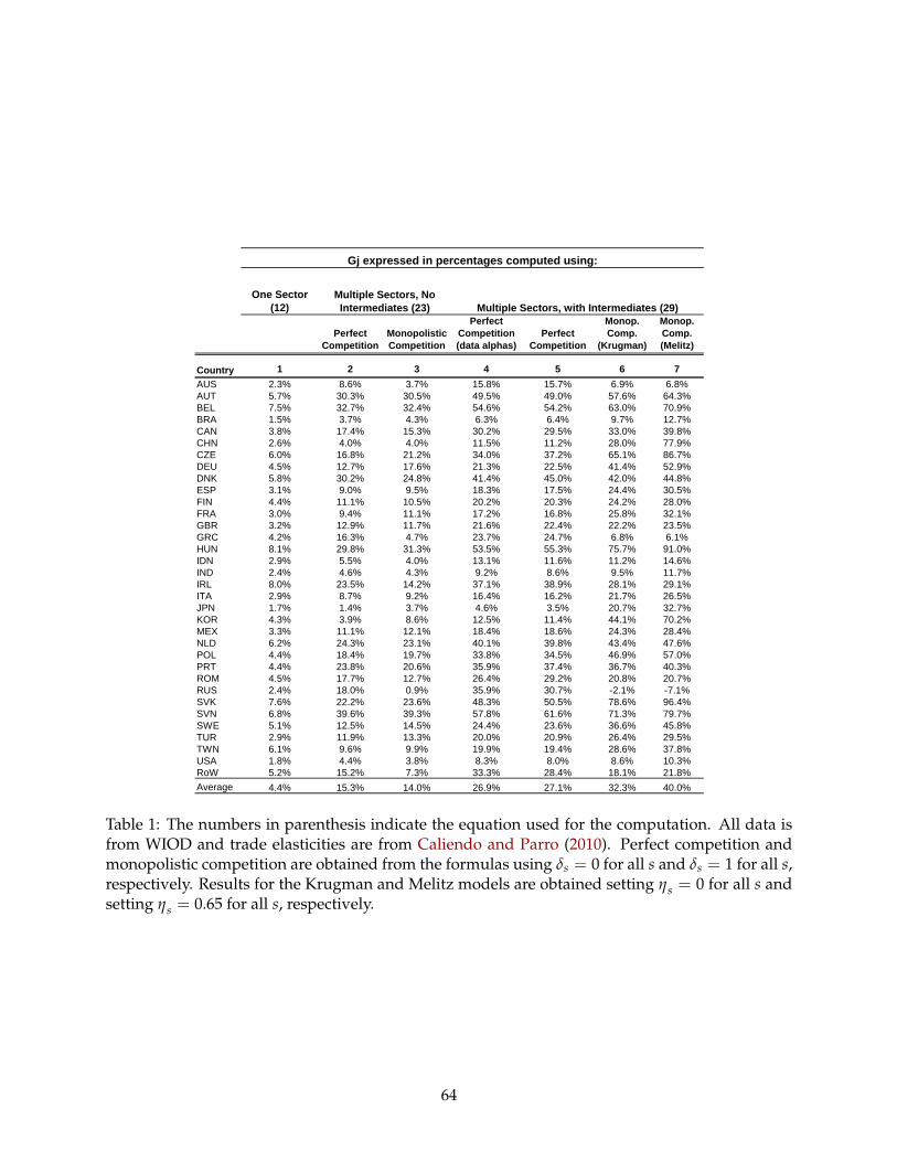
One Sector(12)

PerfectCompetition

MonopolisticCompetition

PerfectCompetition(data alphas)

PerfectCompetition

Monop.Comp.

(Krugman)

Monop.Comp.(Melitz)

Country 1 2 3 4 5 6 7AUS 2.3% 8.6% 3.7% 15.8% 15.7% 6.9% 6.8%AUT 5.7% 30.3% 30.5% 49.5% 49.0% 57.6% 64.3%BEL 7.5% 32.7% 32.4% 54.6% 54.2% 63.0% 70.9%BRA 1.5% 3.7% 4.3% 6.3% 6.4% 9.7% 12.7%CAN 3.8% 17.4% 15.3% 30.2% 29.5% 33.0% 39.8%CHN 2.6% 4.0% 4.0% 11.5% 11.2% 28.0% 77.9%CZE 6.0% 16.8% 21.2% 34.0% 37.2% 65.1% 86.7%DEU 4.5% 12.7% 17.6% 21.3% 22.5% 41.4% 52.9%DNK 5.8% 30.2% 24.8% 41.4% 45.0% 42.0% 44.8%ESP 3.1% 9.0% 9.5% 18.3% 17.5% 24.4% 30.5%FIN 4.4% 11.1% 10.5% 20.2% 20.3% 24.2% 28.0%FRA 3.0% 9.4% 11.1% 17.2% 16.8% 25.8% 32.1%GBR 3.2% 12.9% 11.7% 21.6% 22.4% 22.2% 23.5%GRC 4.2% 16.3% 4.7% 23.7% 24.7% 6.8% 6.1%HUN 8.1% 29.8% 31.3% 53.5% 55.3% 75.7% 91.0%IDN 2.9% 5.5% 4.0% 13.1% 11.6% 11.2% 14.6%IND 2.4% 4.6% 4.3% 9.2% 8.6% 9.5% 11.7%IRL 8.0% 23.5% 14.2% 37.1% 38.9% 28.1% 29.1%ITA 2.9% 8.7% 9.2% 16.4% 16.2% 21.7% 26.5%JPN 1.7% 1.4% 3.7% 4.6% 3.5% 20.7% 32.7%KOR 4.3% 3.9% 8.6% 12.5% 11.4% 44.1% 70.2%MEX 3.3% 11.1% 12.1% 18.4% 18.6% 24.3% 28.4%NLD 6.2% 24.3% 23.1% 40.1% 39.8% 43.4% 47.6%POL 4.4% 18.4% 19.7% 33.8% 34.5% 46.9% 57.0%PRT 4.4% 23.8% 20.6% 35.9% 37.4% 36.7% 40.3%ROM 4.5% 17.7% 12.7% 26.4% 29.2% 20.8% 20.7%RUS 2.4% 18.0% 0.9% 35.9% 30.7% ­2.1% ­7.1%SVK 7.6% 22.2% 23.6% 48.3% 50.5% 78.6% 96.4%SVN 6.8% 39.6% 39.3% 57.8% 61.6% 71.3% 79.7%SWE 5.1% 12.5% 14.5% 24.4% 23.6% 36.6% 45.8%TUR 2.9% 11.9% 13.3% 20.0% 20.9% 26.4% 29.5%TWN 6.1% 9.6% 9.9% 19.9% 19.4% 28.6% 37.8%USA 1.8% 4.4% 3.8% 8.3% 8.0% 8.6% 10.3%RoW 5.2% 15.2% 7.3% 33.3% 28.4% 18.1% 21.8%Average 4.4% 15.3% 14.0% 26.9% 27.1% 32.3% 40.0%

Multiple Sectors, NoIntermediates (23) Multiple Sectors, with Intermediates (29)

Gj expressed in percentages computed using:

Table 1: The numbers in parenthesis indicate the equation used for the computation. All data isfrom WIOD and trade elasticities are from Caliendo and Parro (2010). Perfect competition andmonopolistic competition are obtained from the formulas using δs = 0 for all s and δs = 1 for all s,respectively. Results for the Krugman and Melitz models are obtained setting ηs = 0 for all s andsetting ηs = 0.65 for all s, respectively.

64

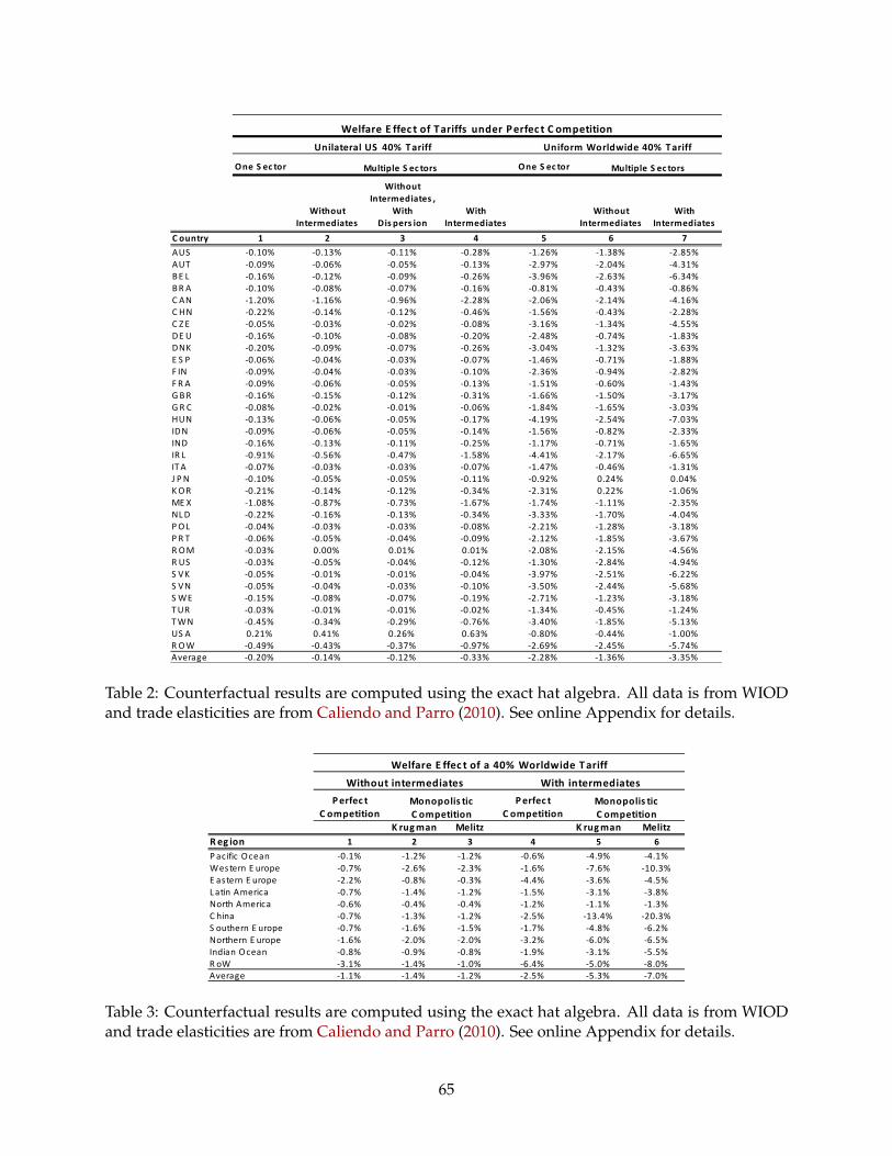
One S ec tor One S ec tor

WithoutIntermediates

WithoutIntermediates ,

WithDis pers ion

WithIntermediates

WithoutIntermediates

WithIntermediates

C ountry 1 2 3 4 5 6 7AUS ­0.10% ­0.13% ­0.11% ­0.28% ­1.26% ­1.38% ­2.85%AUT ­0.09% ­0.06% ­0.05% ­0.13% ­2.97% ­2.04% ­4.31%B E L ­0.16% ­0.12% ­0.09% ­0.26% ­3.96% ­2.63% ­6.34%B R A ­0.10% ­0.08% ­0.07% ­0.16% ­0.81% ­0.43% ­0.86%C AN ­1.20% ­1.16% ­0.96% ­2.28% ­2.06% ­2.14% ­4.16%C HN ­0.22% ­0.14% ­0.12% ­0.46% ­1.56% ­0.43% ­2.28%C Z E ­0.05% ­0.03% ­0.02% ­0.08% ­3.16% ­1.34% ­4.55%DE U ­0.16% ­0.10% ­0.08% ­0.20% ­2.48% ­0.74% ­1.83%DNK ­0.20% ­0.09% ­0.07% ­0.26% ­3.04% ­1.32% ­3.63%E S P ­0.06% ­0.04% ­0.03% ­0.07% ­1.46% ­0.71% ­1.88%F IN ­0.09% ­0.04% ­0.03% ­0.10% ­2.36% ­0.94% ­2.82%F R A ­0.09% ­0.06% ­0.05% ­0.13% ­1.51% ­0.60% ­1.43%G B R ­0.16% ­0.15% ­0.12% ­0.31% ­1.66% ­1.50% ­3.17%G R C ­0.08% ­0.02% ­0.01% ­0.06% ­1.84% ­1.65% ­3.03%HUN ­0.13% ­0.06% ­0.05% ­0.17% ­4.19% ­2.54% ­7.03%IDN ­0.09% ­0.06% ­0.05% ­0.14% ­1.56% ­0.82% ­2.33%IND ­0.16% ­0.13% ­0.11% ­0.25% ­1.17% ­0.71% ­1.65%IR L ­0.91% ­0.56% ­0.47% ­1.58% ­4.41% ­2.17% ­6.65%IT A ­0.07% ­0.03% ­0.03% ­0.07% ­1.47% ­0.46% ­1.31%J P N ­0.10% ­0.05% ­0.05% ­0.11% ­0.92% 0.24% 0.04%K O R ­0.21% ­0.14% ­0.12% ­0.34% ­2.31% 0.22% ­1.06%ME X ­1.08% ­0.87% ­0.73% ­1.67% ­1.74% ­1.11% ­2.35%NL D ­0.22% ­0.16% ­0.13% ­0.34% ­3.33% ­1.70% ­4.04%P O L ­0.04% ­0.03% ­0.03% ­0.08% ­2.21% ­1.28% ­3.18%P R T ­0.06% ­0.05% ­0.04% ­0.09% ­2.12% ­1.85% ­3.67%R O M ­0.03% 0.00% 0.01% 0.01% ­2.08% ­2.15% ­4.56%R US ­0.03% ­0.05% ­0.04% ­0.12% ­1.30% ­2.84% ­4.94%S VK ­0.05% ­0.01% ­0.01% ­0.04% ­3.97% ­2.51% ­6.22%S VN ­0.05% ­0.04% ­0.03% ­0.10% ­3.50% ­2.44% ­5.68%S WE ­0.15% ­0.08% ­0.07% ­0.19% ­2.71% ­1.23% ­3.18%T UR ­0.03% ­0.01% ­0.01% ­0.02% ­1.34% ­0.45% ­1.24%T WN ­0.45% ­0.34% ­0.29% ­0.76% ­3.40% ­1.85% ­5.13%US A 0.21% 0.41% 0.26% 0.63% ­0.80% ­0.44% ­1.00%R O W ­0.49% ­0.43% ­0.37% ­0.97% ­2.69% ­2.45% ­5.74%Average ­0.20% ­0.14% ­0.12% ­0.33% ­2.28% ­1.36% ­3.35%

Welfare E ffec t of Tariffs under P erfec t C ompetitionUnilateral US 40% T ariff

Multiple S ec tors Multiple S ec tors

Uniform Worldwide 40% T ariff

Table 2: Counterfactual results are computed using the exact hat algebra. All data is from WIODand trade elasticities are from Caliendo and Parro (2010). See online Appendix for details.

P erfec tC ompetition

P erfec tC ompetition

K rug man Melitz K rug man MelitzR eg ion 1 2 3 4 5 6P acific O cean ­0.1% ­1.2% ­1.2% ­0.6% ­4.9% ­4.1%Western E urope ­0.7% ­2.6% ­2.3% ­1.6% ­7.6% ­10.3%E astern E urope ­2.2% ­0.8% ­0.3% ­4.4% ­3.6% ­4.5%L atin America ­0.7% ­1.4% ­1.2% ­1.5% ­3.1% ­3.8%North America ­0.6% ­0.4% ­0.4% ­1.2% ­1.1% ­1.3%C hina ­0.7% ­1.3% ­1.2% ­2.5% ­13.4% ­20.3%S outhern E urope ­0.7% ­1.6% ­1.5% ­1.7% ­4.8% ­6.2%Northern E urope ­1.6% ­2.0% ­2.0% ­3.2% ­6.0% ­6.5%Indian O cean ­0.8% ­0.9% ­0.8% ­1.9% ­3.1% ­5.5%R oW ­3.1% ­1.4% ­1.0% ­6.4% ­5.0% ­8.0%Average ­1.1% ­1.4% ­1.2% ­2.5% ­5.3% ­7.0%

Welfare E ffec t of a 40% Worldwide T ariff

Monopolis ticC ompetition

Without intermediates With intermediatesMonopolis ticC ompetition

Table 3: Counterfactual results are computed using the exact hat algebra. All data is from WIODand trade elasticities are from Caliendo and Parro (2010). See online Appendix for details.

65