trade integration and the trade balance in china · trade integration and the trade balance in ......
TRANSCRIPT
Trade Integration and the Trade Balance inChina
George Alessandria Horag Choi Dan Lu
Rochester Monash Rochester
October 2016
https://sites.google.com/site/georgealessandria2/ACL-201606.pdf

Main Question
What accounts for China’s trade balance over last 25 years?
Suspects - productivity, monetary, fiscal, demographic, risk, trade

.2.4
.6.8
trade
y
.05
0.0
5.1
Trad
e Ba
lanc
e R
eal
(%G
DP)
1990 1995 2000 2005 2010 2015
TB/Y
Figure 1: China Real Trade balance

Main Question
What accounts for China’s trade balance dynamics over last 25 years?
Suspects - productivity, monetary, fiscal, demographic, risk, trade
Short Answer: Trade integration key driver
1 Lower trade barriers - easier to run deficits/surpluses
2 Temporary and Asymmetric ∆ in barrier - source ofdeficits/surplus

.2.4
.6.8
trade
y
.05
0.0
5.1
Trad
e Ba
lanc
e R
eal
(%G
DP)
1990 1995 2000 2005 2010 2015
TB/Y Trade/Y
Figure 1: China Real Trade balance & Trade share of GDP
Quadrupling of trade ⇒ big ∆′s in trade barriers/tastes
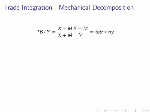
Trade Integration - Mechanical Decomposition
TB/Y =X −MX +M
X +MY
= tbtr ∗ try
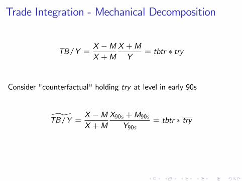
Consider "counterfactual" holding try at level in early 90s
TB/Y =X −MX +M
X90s +M90sY90s
= tbtr ∗ try
Trade Integration - Mechanical Decomposition
TB/Y =X −MX +M
X +MY
= tbtr ∗ try
Consider "counterfactual" holding try at level in early 90s
TB/Y =X −MX +M
X90s +M90sY90s
= tbtr ∗ try
.05
0.0
5.1
1990 1995 2000 2005 2010 2015
TB/Y TB/Y constant trade
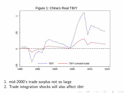
Figure 1: China's Real TB/Y
1. mid-2000’s trade surplus not so large2. Trade integration shocks will also affect tbtr

Preview
Build unified model of China’s growth, trade integration, andborrowing/lending.
I Emphasize changes in trade barriers as source of foreign assetaccumulation
Trade matters for the trade balance when trade cost "shocks"are persistent
I Asymmetric ∆ in trade barriers lead to lendingI Symmetric ∆ in trade barriers lead to net flows with asymmetriccountries
Use model to account for source of integration and dynamics ofintegration
I Trade slowdown primarily reflects lack of additional integrationshocks rather than outright reversal
Model
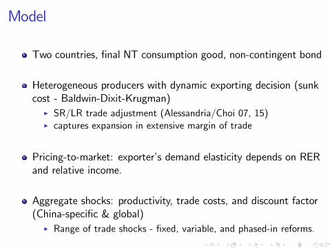
Two countries, final NT consumption good, non-contingent bond
Heterogeneous producers with dynamic exporting decision (sunkcost - Baldwin-Dixit-Krugman)
I SR/LR trade adjustment (Alessandria/Choi 07, 15)I captures expansion in extensive margin of trade
Pricing-to-market: exporter’s demand elasticity depends on RERand relative income.
Aggregate shocks: productivity, trade costs, and discount factor(China-specific & global)
I Range of trade shocks - fixed, variable, and phased-in reforms.
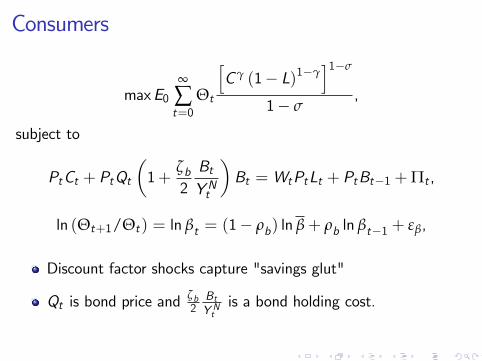
Consumers
maxE0∞
∑t=0
Θt
[Cγ (1− L)1−γ
]1−σ
1− σ,
subject to
PtCt + PtQt
(1+
ζb2BtYNt
)Bt = WtPtLt + PtBt−1 +Πt ,
ln (Θt+1/Θt) = ln βt = (1− ρb) ln β+ ρb ln βt−1 + εβ,
Discount factor shocks capture "savings glut"
Qt is bond price andζb2BtY Nt
is a bond holding cost.
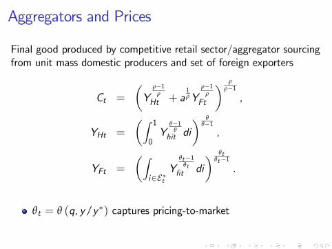
Aggregators and Prices
Final good produced by competitive retail sector/aggregator sourcingfrom unit mass domestic producers and set of foreign exporters
Ct =
(Y
ρ−1ρ
Ht + a1ρY
ρ−1ρ
Ft
) ρρ−1,
YHt =
(∫ 1
0Y
θ−1θ
hit di) θ
θ−1,
YFt =
(∫i∈E∗t
Yθt−1
θtfit di
) θtθt−1
.
θt = θ (q, y/y∗) captures pricing-to-market

Producers - standard sunk cost model (Dixit, 89)
Vt (η,m) = maxm′,p,p∗
pct (p) +m′p∗ct (ξ∗p∗)−Wl
−m′Wfm,t +QtEVt+1(η′,m′
)mit : exporting status from previous period - indexes fixed exportcost
yit = ezt+ηit lit , ηitiid∼ N
(0, σ2η
)ξ∗t > 1: variable trade costs for home exporters
Wt f0,t : sunk cost to start
Wt f1,t : sunk cost to continue.
Trade policy ∆ in shocks to trade costs (ξt , f0,t , f1,t)

Export Entry and Exit Thresholds
∆Vt (η) = Vt (η, 1)− Vt (η, 0)
Wt f0,t − π∗t (η0t) = QtEt∆Vt+1(η′)
Wt f1,t − π∗t (η1t) = QtEt∆Vt+1(η′)
Endogenous entry/exit & hysteresis (η1t < η0t when f1 < f0)
Distribution of exporters is state variable & gradual entry
With iid shocks,
Nt+1 = Pr (η ≥ η1t)Nt + Pr (η ≥ η0t) (1−Nt)

Aggregate Shocks - Productivity
ln z∗t = ρ∗z ln z∗t−1 + ε∗zt , εzt
iid∼ N (0, σ∗z )
ln zdt = ρdz ln zdt−1 + εdzt , εdztiid∼ N
(0, σdz
)ln zt = ln z∗t + ln zd ,t − z
z∗t : Global productivity
zd ,t : China-specific productivity
z : China’s productivity disadvantage.

Aggregate Shocks - Variable Trade Costs
ln ξt = ln ξct + 0.5 ln ξdt ,
ln ξ∗t = ln ξct − 0.5 ln ξdt .
ln ξct =(1− ρξc
)ln ξc + ρξc
ln ξct−1 + ln ξgt−1 + εξc t ,
ln ξgt = ρξgln ξgt−1 + εξg t ,
ln ξdt =(1− ρξd
)ln ξd + ρξd
ln ξdt−1 + εξd t .
Transitory: ξct : common shock and ξdt : differential shocksTrend common shocks. news aspect - know one-year in advancepath of liberalization.

Aggregate Shocks - Fixed Trade Costs
ln f0t = (1− ρf 0) ln f0 + ρf 0 ln f0t−1 + εf 0,t ,
ln f1t = (1− ρf 1) ln f1 + ρf 1 ln f1t−1 + εf 1,t .
Constrain ρf 1 = ρf 0 = ρf

Calibration/Estimation
Fixed Parameters
β ζb γ a1 θ0.96 0.0001 0.30 0.16 5
Estimate
Shock process: zc , zd , ξc , ξg , ξd , f0, f1, b
Level of trade costs(ξc ξd , f0, f1
)and technology
(z, ση
)Preferences
(σ, ρ, ζq , ζy
)
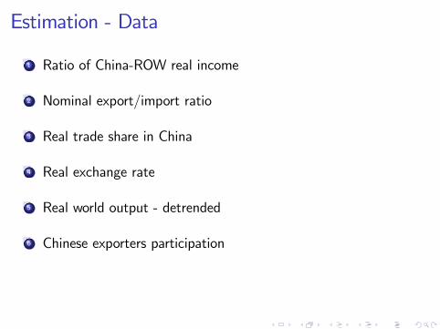
Estimation - Data
1 Ratio of China-ROW real income
2 Nominal export/import ratio
3 Real trade share in China
4 Real exchange rate
5 Real world output - detrended
6 Chinese exporters participation

5 10 15 20 250
0.1
0.2Y _ c h in a /Y _ ro w (% )
5 10 15 20 250.8
1
1.2
1.4C h in a E x p o rtIm p o rt R a tio (N o m in a l)
5 10 15 20 250.2
0.4
0.6
0.8R e a l T ra d e s h a re C h in a (X + M )/Y
5 10 15 20 250.5
0
0.5R e a l E x c h a n g e R a te (lo g )
5 10 15 20 250.1
0
0.1W o rld O u tp u t
5 10 15 20 250.1
0.2
0.3
0.4C h in e s e E x p o rte rs (% )
Historical and Smoothed Series
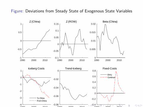
Figure: Deviations from Steady State of Exogenous State Variables
1990 2000 20101
0.5
0
0.5
1Z (China)
1990 2000 20100.1
0.05
0
0.05
0.1
0.15Z (ROW)
1990 2000 20100
0.005
0.01
0.015
0.02Beta (China)
1990 2000 20104
3
2
1
0
1Iceberg Costs
To ChinaFrom China
1990 2000 20100.08
0.06
0.04
0.02
0TrendIceberg
1990 2000 20100.4
0.2
0
0.2
0.4
0.6
0.8FixedCosts
EntryContinue

Estimated Persistence of Shocksprior posterior 90% HPD - interval prior priormean mean mode std.dev.
ρzd 0.95 0.996 0.999 0.9905 - 1 unif 0.5ρzc 0.7 0.747 0.731 0.5586 - 0.954 unif 0.5ρξc
0.79 0.917 0.962 0.8099 - 0.9981 unif 0.5
ρξd0.95 0.978 0.992 0.9578 - 0.9998 unif 0.5
ρb 0.945 0.948 0.953 0.9158 - 0.98 norm 0.025ρξg
0.8 0.895 0.975 0.7423 - 0.9978 unif 0.5
ρf 0.9 0.820 0.853 0.666 - 0.9939 unif 0.5ρ 2 1.7975 1.8167 1.5194-2.0776 invg 1σ 5 4.7777 4.4192 3.3591-5.9876 invg 1
Notes: Based on annual data from 1990 to 2014.
Shocks are persistent but not permanent - rationale forborrowing/lending

Nominal Export-Import Ratio and Trade Shocks
Consider 1 standard deviation shock that increase trade
Differential trade shock - relatively cheaper for China to export -relatively large impact on net trade flows and weak effect ongross flows

0 5 10 15 20 250
0.005
0.01
0.015
0.02
0.025
0.03
0.035
0.04
0.045
0.05China Trade Share
0 5 10 15 20 250.02
0.015
0.01
0.005
0
0.005
0.01
0.015
0.02
0.025
0.03c. Nominal ExportImport Ratio
c
d
g

Nominal Export-Import Ratio and Trade Shocks
Consider 1 standard deviation shock that increase trade
Differential trade shock - relatively cheaper for China to export -relatively large impact on net trade flows and weak effect ongross flows
Global shocks have an effect on net trade since countries are ofdifferent sizes and hence they have wealth effects
I Persistent shock- China saves to smooth out shock
I Trend shock - China borrows against future

0 5 10 15 20 250
0.005
0.01
0.015
0.02
0.025
0.03
0.035
0.04
0.045
0.05China Trade Share
0 5 10 15 20 250.02
0.015
0.01
0.005
0
0.005
0.01
0.015
0.02
0.025
0.03c. Nominal ExportImport Ratio
c
d
g

Decomposition of Trade Balance to GDP
Construct contribution of shocks to Trade-Balance/GDP fromcontribution to Export-Import Ratio and Trade-GDP Ratio
I Need to account for direct and interaction effects (i.e. discountfactor shock has bigger impact with a trade cost shock)
I Group shocks into trade costs (T), productivity & preferences(P), and Initial Conditions (I)

a. TB/Y (Nominal)
0.06
0.04
0.02
0.00
0.02
0.04
0.06
0.08
0.10
1990 1995 2000 2005 2010
I
P
T
IxP
IxT
PxT
IxPxT
All
Data
Trade costs were major source of surpluses in since 2003.

Decomposition of Net Foreign Assets to GDP Ratio
Construct contribution of shocks to NFA/GDP by accumulatingTB
Specifically, take model’s initial assets to GDP(Q1990B1990/Y1990) and then update QtBt/Yt using the law ofmotion
QtBtYNt
=
(Qt−1Bt−1YNt−1
)(1
Qt−1
)(YNt−1YNt
)+0.5 ln (XNt/MNt)
YNt,
I Again need to account for direct and interaction effects

b. Net Foreign Assets/GDP
0.60
0.40
0.20
0.00
0.20
0.40
0.60
0.80
1.00
1.20
1990 1995 2000 2005 2010
I
P
T
IxP
IxT
PxT
IxPxT
All
Data
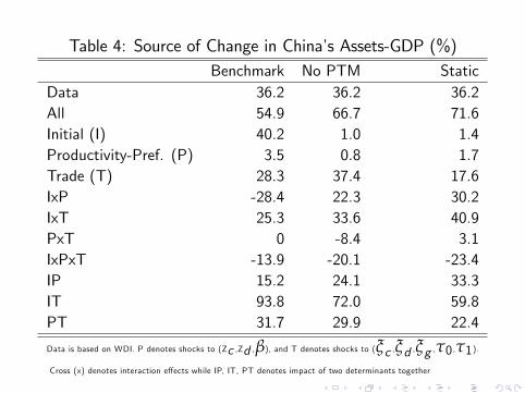
Table 4: Source of Change in China’s Assets-GDP (%)Benchmark No PTM Static
Data 36.2 36.2 36.2All 54.9 66.7 71.6Initial (I) 40.2 1.0 1.4Productivity-Pref. (P) 3.5 0.8 1.7Trade (T) 28.3 37.4 17.6IxP -28.4 22.3 30.2IxT 25.3 33.6 40.9PxT 0 -8.4 3.1IxPxT -13.9 -20.1 -23.4IP 15.2 24.1 33.3IT 93.8 72.0 59.8PT 31.7 29.9 22.4
Data is based on WDI. P denotes shocks to (Zc ,Zd ,β), and T denotes shocks to (ξc ,ξd ,ξg ,τ0 ,τ1).Cross (x) denotes interaction effects while IP, IT, PT denotes impact of two determinants together

Global Trade SlowdownFollowing Trade collapse and recovery global trade integration hasbeen anemic -
1990 1995 2000 2005 2010 20150.2
0.3
0.4
0.5
0.6
0.7
0.8China Real Trade Share (%)
1990 1995 2000 2005 2010 20150.02
0.04
0.06
0.08
0.1
0.12
0.14
0.16
0.18World Trade (%)
Is this the end of integration or a reversal?
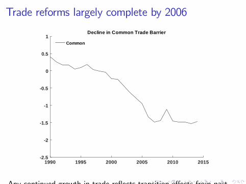
Trade reforms largely complete by 2006
1990 1995 2000 2005 2010 20152.5
2
1.5
1
0.5
0
0.5
1Decline in Common Trade Barrier
Common
Any continued growth in trade reflects transition effects from pastreforms
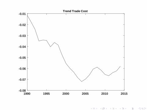
1990 1995 2000 2005 2010 20150.08
0.07
0.06
0.05
0.04
0.03
0.02
0.01Trend Trade Cost

Static vs Dynamic Trade Model: Expected TradeGrowth
Consider how estimated future trade costs depend on model
Eliminate sunk cost - static exporting model
Re-estimate model with 1 fixed export cost f0 = f1

1990 1995 2000 2005 2010 20150.045
0.04
0.035
0.03
0.025
0.02
0.015
0.01
0.005
0Iceberg cost Trend growth (Change from 1990)
BenchmarkStatic
Integration prospects overstated in static models

Summary
Changes in trade barriers matter for change in net foreign assets
Chinese trade integration attributed equally to trend, common,differential and productivity.
Trade slow-down mostly reflects lack of barrier reductions, ratherthan reversal, and waning influence of past reforms.
I Expectations for integration have diminished but remain similarto 1999 levels

Estimated Preferences and Technologyprior posterior 90% HPD Interval prior priormean mean mode std.dev.
q -1 -1.0459 -1.0518 -1.3639 -0.6777 norm 0.25Yw -1.335 -1.3198 -1.3273 -1.3958 -1.2479 norm 0.2
ρ 2 1.7975 1.8167 1.5194 2.0776 invg 1σ 5 4.7777 4.4192 3.3591 5.9876 invg 1z 2.42 2.338 2.3449 2.1749 2.4864 norm 0.1
ξc 0.5 0.5031 0.5045 0.4251 0.5742 norm 0.05ξd 0.1 0.1132 0.1001 -0.0379 0.2631 norm 0.1ςq 0 0.0364 0.0526 -0.1515 0.2441 norm 0.15ςy 0 -0.0203 -0.0275 -0.113 0.0888 norm 0.15f0 0.37 0.3786 0.3681 0.2969 0.4545 invg 0.05f1 0.04 0.0422 0.0428 0.0348 0.0498 invg 0.005
ση 0.235 0.199 0.186 0.1508 0.2434 invg 0.05
Notes: Based on annual data from 1990 to 2014.

Estimated Shock Std. Deviationprior posterior 90% HPD - interval prior priormean mean mode std.dev.
σzd 0.07 0.0699 0.0678 0.0527 - 0.0871 invg 0.025σzc 0.033 0.0355 0.0333 0.0267 - 0.043 invg 0.025σξc
0.2 0.1602 0.1549 0.1209 - 0.1984 invg 0.05σξd
0.124 0.1653 0.1531 0.1276 - 0.2018 invg 0.05σξg
0.016 0.0339 0.0118 0.0052 - 0.0692 invg 0.02
σf0 0.01 0.007 0.0047 0.0025 - 0.0119 invg 0.05σf1 0.22 0.2213 0.2193 0.2075 - 0.2378 invg 0.01σb 0.005 0.0055 0.0044 0.0029 - 0.0082 invg 0.01
Notes: Based on annual data from 1990 to 2014.

Period is 1990 to 2014

Outline
Model
Estimation
Results - decomposition of
I Net Foreign Assets
I Trade Integration
I Trade Slowdown

Assets-GDP Ratio and Trade cost shocks
Consider 1 standard deviation shock
Persistent trade cost shocks ∆ assets.
Common increase in trade cost affects China more since it ismore open.
I + transitory →borrowing
I + trend shock →savings
Differential shocks, temporarily cheaper for ROW toconsume→savings
Fixed cost shock: temporarily more expensive for ROW toconsume→borrow